Unexorcized ghost in DGP brane world

Abstract

The brane world model proposed by Dvali-Gabadadze-Porrati realizes self-acceleration of the universe. However, it is known that this cosmological solution contains a spin-2 ghost. We study the possibility of avoiding the appearance of the ghost by slightly modifying the model via the introduction of a second brane. First, we consider a simple model without stabilization of the brane separation. By changing the separation between the branes, we find that we can erase the spin-2 ghost. However, this can be done only at the expense of the appearance of a spin-0 ghost instead. We discuss why these two different types of ghosts are correlated. Then, we examine a model with stabilization of the brane separation. Even in this case, we find that the correlation between spin-0 and spin-2 ghosts remains. As a result we find that we cannot avoid the appearance of a ghost by introducing a second brane in the model.

I Introduction

The observed present-day accelerated expansion of the universe SN is one of the hottest topics in cosmology. There are two aspects in this issue: The first is to explain the late-time accelerated expansion of the universe, and the second is to explain why the accelerated expansion began only recently. There have been many attempts to modify standard cosmological models in order to address these problems. As far as we know, none of these give a natural solution to the second problem. To give a solution to the second problem, one may need to combine ideas which solve the first problem with the anthropic principle anth .

In this paper, our interest is in the first problem. Most of ideas that solve the first problem are modifications of the scalar (spin-0) sector of the cosmological model, such as introduction of a cosmological constant const or quintessence quint . But there is another direction which has not been explored much so far. That is modifying the gravity theory in the spin-2 sector.

The simplest model with a modified spin-2 sector involves massive gravity FP . Since models which have terms quadratic in metric perturbations can be regarded as a massive gravity theories, most modified gravity models fall into this category. If we introduce the mass of the graviton to explain the accelerated expansion of the universe, its value would be the same order as the present value of the Hubble parameter, $m_{g}\simeq H$. However, it is known that a spin-2 graviton with mass in the range $0<m^{2}<2H^{2}$ in de Sitter background has a ghost excitation in its helicity-0 component Higuchi . The Hubble parameter is larger in an earlier epoch of the universe. Hence it seems difficult to avoid the appearance of a ghost throughout the evolution of the universe in simple models that attempt to explain the present-day accelerated expansion. Here we would like to raise a simple question: Can we build a model, incorporating modification of the spin-2 sector, that explains the accelerated cosmic acceleration and is ghost-free?

The DGP brane world model DGP (See Ref. Lue for a recent review paper), in which the 4D Einstein-Hilbert action is assumed to be induced on the brane, is a mechanism to realize the late-time accelerated expansion of the Universe without introducing additional matter self . Such a solution is called the self-accelerating branch. This is in contrast to the normal branch, where there is no cosmic expansion in the limit of vanishing matter energy density. There are many investigations of the DGP model, such as spherically symmetric solutions SSS ; Lue2 , analyses of structure formation SF and shock wave limits SW . In quantizing the theory, we face the issue of strong coupling strong ; SG , which is the problem that nonlinear effects of the scalar gravitational interaction become important below some unexpectedly large length scale. Moreover, the existence of a ghost excitation has been pointed out in the self-accelerating branch of the DGP brane world model SG ; Koyama ; Koyama2 . We here discuss this ghost problem. By considering perturbations around this solution, a Kaluza-Klein tower of massive gravitons in the four dimensional effective theory is obtained. The lowest mass $m$ satisfies $m^{2}=2H^{2}$ Koyama ; Koyama2 . If the analogy to the massive gravity theory holds, this would mean that the self-accelerating branch of the DGP model does not have a ghost excitation. However, it a detailed analysis has shown that there is still a ghost in this model Koyama2 .

In this paper, based on the DGP brane world model, we attempt to build a ghost-free model which simultaneously explains the accelerated expansion of the universe due to effects in the spin-2 sector. The first idea is to increase the lowest graviton mass by introducing a boundary brane. We call this the two-brane model, which is successful in making all graviton masses satisfy $2H^{2}<m^{2}$. However, a spin-0 excitation, which originates from the brane bending degrees of freedom, is transmuted into a ghost. We will find that a ghost excitation cannot be eliminated in this two-branes model.

Usually spin-2 modes are decoupled from spin-0 modes at the level of linear perturbations. Therefore it seems mysterious that the disappearance of the spin-2 ghost coincides with the appearance of a spin-0 ghost. The magic is in that a spin-2 mode can be obtained from a spin-0 mode by applying a differential operator if and only if the mass squared takes a specific critical value. At the critical mass, a spin-2 mode can couple with a spin-0 mode. In addition, the critical mass corresponds to a threshold for the appearance of a ghost in the spin-2 sector. If the mass of a spin-2 mode is smaller than the critical mass, the spin-2 sector has a ghost excitation as previously mentioned. Moreover, a unique spin-0 mode that appears in the two-branes model has also the critical mass. Hence the spin-2 mode can couple with the spin-0 mode when it crosses the critical mass. This fact partly explains why the ghost can be transferred between the spin-2 and spin-0 sectors.

Then, we consider a model with stabilized brane separation by introducing a bulk scalar field into the two-branes model GW ; TM . Since the mass spectrum of spin-0 modes changes, the spin-0 mode at the critical mass does not survive in this stabilized two-branes model. Then, it is expected that the ghost will not be transferred between the spin-2 and spin-0 sectors. However, by studying this stabilized two-branes model in detail, we will find that this naive expectation is wrong.

This paper is organized as follows. In §II we will discuss the two-branes model. In §III extension to the stabilized two-branes model is performed. We will summarize our results in §IV.

II Two-branes model

As mentioned in Introduction, it is known that in de Sitter spacetime a massive spin-2 field whose mass squared is less than $2H^{2}$ has a ghost Higuchi , where $H$ is the Hubble parameter. The self-accelerating branch of the DGP brane world model DGP ; self has a spin-2 excitation whose mass squared is $2H^{2}$. In the usual massive graviton model with Fierz-Pauli mass term, this is a special case where a helicity-0 excitation disappears Higuchi ; Deser . However, a detailed analysis reveals that there is a ghost mode in the self-accelerating branch of DGP model due to the existence of a spin-0 excitation Koyama2 . Since the ghost arises due to a subtle mechanism in this model, it would be a natural question whether one can eliminate the ghost by a slight modification of this model or not.

In this section we examine the two-branes model with a boundary brane in the bulk as one of the simplest extensions of original DGP scenario. Our initial expectation is as follows: The new boundary will shift the mass of spin-2 modes. Then we will be able to construct models with no spin-2 excitations with masses in the range that implies the existence of a ghost.

However, we will find later that spin-0 excitations, which correspond to the brane bending degrees of freedom, carry a ghost mode instead. It will turn out to be impossible to eliminate the ghost by this simple two-branes extension. Below, we discuss how the ghost is transferred between the spin-2 and spin-0 sectors Kaloper .

II.1 Background

As mentioned above, in order to obtain a model that does not have spin-2 ghost modes, we introduce another brane into the DGP model. The action is

$$S={1\over 2\kappa^{2}}\int d^{5}x\sqrt{-g}R+\sum_{\sigma=\pm}\int d^{4}x\sqrt{-g^{(4)}_{\sigma}}\left({1\over 2\kappa_{4}^{2}}R^{(4)}_{\sigma}+{1\over\kappa^{2}}K_{\sigma}-\tau_{\sigma}+L_{m\sigma}\right),$$ (1)

where $R$, $R^{(4)}_{\pm}$, $g^{(4)}_{\pm}$, $K_{\pm}$, $\tau_{\pm}$ and $L_{m\pm}$ are the five dimensional Ricci scalar, four dimensional Ricci scalar, trace of the four dimensional induced metric $g_{\mu\nu}$, trace of the extrinsic curvature $K_{\mu\nu}$, the brane-tension, and the matter Lagrangian on the $(\pm)$-branes, respectively. Assuming $Z$₂ symmetry across each brane, the junction conditions to be imposed at each brane are

$$K_{\pm\mu\nu}=r_{c}\left[-\kappa^{2}\left(T^{(\pm)}_{\mu\nu}-\frac{1}{3}T^{(\pm)}g_{\mu\nu}\right)+\left(G_{\pm\mu\nu}-\frac{1}{3}G_{\pm}g_{\mu\nu}\right)\right],$$ (2)

with $r_{c}:=\kappa^{2}/2\kappa_{4}^{2}$.

We assume vacuum without any matter field, $L_{m\sigma}=0$, as an unperturbed state. The five dimensional metric is given by

$$ds^{2}=dy^{2}+a^{2}(y)\gamma_{\mu\nu}dx^{\mu}dx^{\nu},$$ (3)

with two boundary four dimensional de Sitter ($\pm$)-branes, where $\gamma_{\mu\nu}$ is the four dimensional de Sitter metric with unit curvature radius and the warp factor $a(y)$ is given by

$$a(y)=a_{+}+y.$$ (4)

The range of $y$-coordinate is from $0$ to $(a_{-}-a_{+})$. The positions of $(+)$ and $(-)$-branes are at $y=y_{+}:=0$ and at $y=y_{-}:=a_{-}-a_{+}$, respectively. In the present model, the value of the warp factor on the brane is related to the Hubble parameters evaluated on each brane $H_{\pm}$ as $a_{\pm}=1/H_{\pm}$. Notice that the bulk geometry of the above solution is nothing but the five dimensional Minkowski spacetime written in the spherical Rindler coordinates. From the junction conditions (2), the Hubble parameters on the respective branes are related to the tension of the branes as

$$\pm H_{\pm}=r_{c}H^{2}_{\pm}-\frac{\kappa_{4}^{2}}{6}\tau_{\pm},\qquad\mbox{with}\quad H_{+}>H_{-}\geq 0.$$ (5)

II.2 Perturbation equations

Now we study perturbations around the background mentioned above. Besides the transverse-traceless conditions, one can impose the conditions of vanishing $\{yy\}$ and $\{y\mu\}$-components of metric perturbations. Then the perturbed metric is given by

$$ds^{2}=dy^{2}+\left(a^{2}\gamma_{\mu\nu}+h^{(TT)}_{\mu\nu}\right)dx^{\mu}dx^{\nu},$$ (6)

with

$$\nabla^{\mu}h^{(TT)}_{\mu\nu}=0,\quad h^{(TT)\mu}_{~{}~{}~{}~{}\mu}=0,$$ (7)

where $\nabla_{\mu}$ is the covariant derivative operator associated with $\tilde{\gamma}_{\mu\nu}:=a^{2}\gamma_{\mu\nu}$. In raising or lowering Greek indices, we use $\tilde{\gamma}_{\mu\nu}$. The $\{\mu\nu\}$-components of the Einstein equations in the bulk are

$$a^{2}h^{\prime\prime(TT)}_{\mu\nu}-2h^{(TT)}_{\mu\nu}=-(\Box^{(4)}-2)h^{(TT)}_{\mu\nu},$$ (8)

where a prime “$~{}^{\prime}~{}$” denotes a partial differentiation with respect to $y$, and $\Box^{(4)}:=\gamma^{\mu\nu}\nabla_{\mu}\nabla_{\nu}$.

In this gauge, branes do not in general reside at fixed values of $y$. We denote the locations of the branes by $y=y_{\pm}+\hat{\xi}^{(5)}_{\pm}(x^{\mu})$. To study the boundary conditions, it is convenient to introduce two sets of new “Gaussian normal” coordinates associated with respective branes. Here “Gaussian normal” means coordinates such that $\{y\mu\}$-components vanish and the location of each brane is specified by a constant $y$-surface. Notice that the “Gaussian normal” coordinates associated with $(+)$-brane in general differ from those associated with $(-)$-brane. In these coordinates the junction conditions imposed on the branes is simple. We associate an over-bar “$\,\bar{~{}}\,$” with the perturbation variables in these coordinates.

The junction conditions for metric perturbations in the “Gaussian normal” coordinates are

$$\pm\bar{h}^{(\pm)}_{\mu\nu}{}^{\prime}\mp 2H_{\pm}\bar{h}^{(\pm)}_{\mu\nu}=-\kappa^{2}\left[T^{(\pm)}_{\mu\nu}-\frac{1}{3}\tilde{\gamma}_{\mu\nu}T^{(\pm)}\right]+2r_{c}\left[X^{(\pm)}_{\mu\nu}-{1\over 3}\tilde{\gamma}_{\mu\nu}X^{(\pm)}\right],$$ (9)

with

$$X^{(\pm)}_{\mu\nu}:=-\frac{1}{2}\left(a^{-2}\Box^{(4)}\bar{h}^{(\pm)}_{\mu\nu}-\nabla_{\mu}\nabla_{\alpha}\bar{h}^{(\pm)\alpha}_{\,~{}~{}\nu}-\nabla_{\nu}\nabla_{\alpha}\bar{h}^{(\pm)\alpha}_{\,~{}~{}\mu}+\nabla_{\mu}\nabla_{\nu}\bar{h}^{(\pm)}\right)$$

$$\qquad\qquad\qquad-\frac{1}{2}\tilde{\gamma}_{\mu\nu}\left(\nabla_{\alpha}\nabla_{\beta}\bar{h}_{(\pm)}^{\alpha\beta}-a^{-2}\Box^{(4)}\bar{h}^{(\pm)}\right)+a^{-2}\left(\bar{h}^{(\pm)}_{\mu\nu}+\frac{1}{2}\tilde{\gamma}_{\mu\nu}\bar{h}^{(\pm)}\right).$$ (10)

Here $T^{(\pm)}:=\tilde{\gamma}^{\mu\nu}T^{(\pm)}_{\mu\nu}$ and $X^{(\pm)}$ is defined in the same manner. The generators of the gauge transformation from the “Gaussian normal” coordinates to the Newton gauge are given by

$$\xi_{(\pm)}^{y}:=y-\bar{y}=\hat{\xi}^{y}_{(\pm)}(x^{\mu}),$$

and

$$\xi_{(\pm)}^{\mu}:=x^{\mu}-\bar{x}^{\mu}={1\over a}\gamma^{\mu\nu}\partial_{\nu}\hat{\xi}^{y}_{(\pm)}(x^{\rho})+\hat{\xi}^{\mu}_{(\pm)}(x^{\rho}).$$

By this gauge transformation, the metric perturbations transform as

$$\bar{h}^{(\pm)}_{\mu\nu}(y)=h^{(TT)}_{\mu\nu}(y)-2a\left(1-aH_{\pm}\right)\nabla_{\mu}\nabla_{\nu}\hat{\xi}^{y}_{(\pm)}-2a\gamma_{\mu\nu}\hat{\xi}^{y}_{(\pm)}(x^{\rho}),$$ (11)

where we have chosen $\hat{\xi}^{\mu}_{(\pm)}$ so that the second term in (11) vanishes on the brane. Substituting (11) into the traceless part of Eq. (9), the perturbed junction conditions for $h^{(TT)}_{\mu\nu}$ imposed at $y=y_{\pm}$ becomes

$$\pm h^{\prime(TT)}_{\mu\nu}\mp 2H_{\pm}h^{(TT)}_{\mu\nu}+r_{c}H^{2}_{\pm}\left(\Box^{(4)}-2\right)h^{(TT)}_{\mu\nu}=-\kappa^{2}\Sigma^{(\pm)}_{\mu\nu},$$ (12)

with

$$\Sigma^{(\pm)}_{\mu\nu}=\left(T^{(\pm)}_{\mu\nu}-\frac{1}{4}\tilde{\gamma}^{\pm}_{\mu\nu}T^{(\pm)}\right)\pm\frac{2}{\kappa^{2}}(1\mp 2H_{\pm}r_{c})\left(\nabla_{\mu}\nabla_{\nu}-\frac{1}{4}\gamma_{\mu\nu}\Box^{(4)}\right)\hat{\xi}^{y}_{(\pm)},$$ (13)

where $\tilde{\gamma}^{+}_{\mu\nu}:=\tilde{\gamma}_{\mu\nu}|_{y=y_{+}}$. Combining the bulk equations and the junction conditions, we finally obtain

$$\left[\hat{L}^{(TT)}+\frac{\Box^{(4)}\!-2}{a^{2}}\right]h^{(TT)}_{\mu\nu}(y)=\sum_{\sigma=\pm}\left(-2\kappa^{2}\Sigma^{(\sigma)}_{\mu\nu}-2r_{c}H^{2}_{\sigma}\left(\Box^{(4)}\!-2\right)h^{(TT)}_{\mu\nu}(y_{\sigma})\right)\delta(y-y_{\sigma}),$$ (14)

where

$$\hat{L}^{(TT)}:={1\over a^{2}}\partial_{y}a^{4}\partial_{y}{1\over a^{2}}.$$ (15)

The trace part of Eq. (9) gives

$$\left(\Box^{(4)}\!+4\right)\hat{\xi}^{y}_{(\pm)}=\pm\frac{\kappa^{2}}{6H_{\pm}^{2}(1\mp 2r_{c}H_{\pm})}T^{(\pm)}.$$ (16)

The source $\Sigma^{(\pm)}_{\mu\nu}$ should also satisfy the transverse conditions, which can be shown to be identical to the condition (16) by using the identity,

$$\nabla^{\mu}\left(\nabla_{\mu}\nabla_{\nu}-\frac{1}{4}\gamma_{\mu\nu}\Box^{(4)}\right)Y\equiv{3\over 4}\nabla_{\nu}\left(\Box^{(4)}\!+4\right)Y,$$ (17)

which holds for an arbitrary scalar function $Y$.

II.3 Solution with source

Equations (14) are separable. We define a complete set of functions of $y$ by (real-valued) eigen-functions of the eigenvalue equation associated with (14),

$$\left[\frac{m_{i}^{2}}{a^{2}}\left(1+2r_{c}\sum_{\sigma=\pm}\delta(y-y_{\sigma})\right)\right]u_{i}(y)=-\hat{L}^{(TT)}u_{i}(y),$$ (18)

where $m_{i}^{2}$ is the eigenvalue, which we find corresponds to $\Box^{(4)}-2$ in comparison with Eq. (14). Then, thus defined eigen-functions are mutually orthogonal with respect to the inner product defined by

$$(u_{i},u_{j})^{(TT)}:=\oint\frac{d\tilde{y}}{a^{2}}\left(1+2r_{c}\sum_{\sigma=\pm}\delta(y-y_{\sigma})\right)u_{i}(y)u_{j}(y),$$ (19)

where the integral is taken over a twofold covering coordinate $\tilde{y}$ which ranges from $-(y_{-}-y_{+})$ to $+(y_{-}-y_{+})$ and is related to $y$ by $y=|\tilde{y}|$. Both ends of the range of $\tilde{y}$ are identified. By definition, the norm $(u_{i},u_{i})^{(TT)}$ is positive definite. We normalize the eigen-functions so that they satisfy $(u_{i},u_{j})^{(TT)}=\delta_{ij}$.

Expanding $h^{(TT)}_{\mu\nu}$ in terms of these eigen-functions as

$$h^{(TT)}_{\mu\nu}=\sum_{j}h_{\mu\nu}^{(j)}(x^{\mu})u_{j}(y),$$ (20)

the equations of motion (14) reduce to

$${1\over a^{2}}\sum_{j}\left(\Box^{(4)}\!-2-m_{j}^{2}\right)\left(1+2r_{c}\sum_{\sigma=\pm}\delta(y-y_{\sigma})\right)h_{\mu\nu}^{(j)}(x^{\mu})u_{j}(y)=-2\kappa^{2}\Sigma^{(+)}_{\mu\nu}\delta(y-y_{+}),$$ (21)

where we have assumed that the source is only on the $(+)$-brane. Operating $(\oint d\tilde{y}\,u_{i}(y)\times)$ on both sides of the above equations, we obtain

$$(\Box^{(4)}\!-2-m_{i}^{2})h_{\mu\nu}^{(i)}(x^{\mu})=-2\kappa^{2}\Sigma^{(+)}_{\mu\nu}u_{i}(y_{+}).$$ (22)

Hence, the solution for $h_{\mu\nu}$ becomes

$$h_{\mu\nu}^{(TT)}(y)=-2\kappa^{2}\sum_{i}{u_{i}(y_{+})u_{i}(y)\over\Box^{(4)}\!-2-m_{i}^{2}}\Sigma^{(+)}_{\mu\nu}.$$ (23)

From (11) with the aid of (16) and (23), the induced metric on the $(+)$-brane for the solution with source is given by

$$\bar{h}^{(+)}_{\mu\nu} = -2\kappa^{2}\sum_{i}{u_{i}^{2}(y_{+})\over\Box^{(4)}-2-m_{i}^{2}}\left(T_{\mu\nu}^{(+)}-{1\over 4}\tilde{\gamma}_{\mu\nu}T^{(+)}+{H_{+}^{-2}\over 3(m_{i}^{2}-2)}\left(\nabla_{\mu}\nabla_{\nu}-{1\over 4}\gamma_{\mu\nu}\Box^{(4)}\right)T^{(+)}\right)$$ (25)

$$+\frac{\kappa^{2}}{6H_{+}^{2}}\gamma_{\mu\nu}\left({2\over H_{+}}(2r_{c}H_{+}-1)^{-1}-\left(\sum_{i}\frac{u_{i}^{2}(y_{+})}{m_{i}^{2}-2}\right){\Box^{(4)}}\right){1\over\Box^{(4)}+4}T^{(+)},$$

where we have neglected terms which can be erased by a gauge transformation, and we have used the relation

$${1\over\Box^{(4)}\!-2-m^{2}}\left(\nabla_{\mu}\nabla_{\nu}-{1\over 4}\gamma_{\mu\nu}\Box^{(4)}\right)Y=\left(\nabla_{\mu}\nabla_{\nu}-{1\over 4}\gamma_{\mu\nu}\Box^{(4)}\right){1\over\Box^{(4)}\!-m^{2}+6}Y,$$ (26)

which holds for an arbitrary scalar function $Y$. This relation is equivalent to the identity

$$\left(\nabla_{\mu}\nabla_{\nu}\Box^{(4)}-\Box^{(4)}\nabla_{\mu}\nabla_{\nu}\right)Y\equiv-8\left(\nabla_{\mu}\nabla_{\nu}-{1\over 4}\gamma_{\mu\nu}\Box^{(4)}\right)Y.$$ (27)

Note that we have also used the relation

$$\frac{1}{(\Box^{(4)}-2-m_{i}^{2})(\Box^{(4)}-4)}=\frac{1}{m_{i}^{2}-2}\left(\frac{1}{\Box^{(4)}-2-m_{i}^{2}}-\frac{1}{\Box^{(4)}-4}\right),$$ (28)

which cannot be applied when $m_{i}^{2}=2$.

We stress that when $m_{i}^{2}=2$, there is no pathology present in the model, in contrast to the Fierz-Pauli case. In the Fierz-Pauli model, we cannot put the matter with $T\neq 0$ if the squared mass is set to $2H^{2}$, because the equation of motion implies that $T=0$ (see Eq. (109) in the Appendix). However, in the DGP brane world model there is no such a restriction. When the DGP brane world action is reduced to the form of Eq. (25), there appears to be a similar pathology. However, this naive guess is wrong since Eq. (25) is derived by using Eq. (28), which is not correct when $m_{i}^{2}=2$. When we go back to more basic equations (23) and (16), it is easy to find that the matter with $T\neq 0$ can be consistently introduced into the DGP brane world even if $m_{i}^{2}=2$. The seemingly pathological expression (25) at $m_{i}^{2}=2$ is due to the decomposition to spin-2 and spin-0 perturbations (28).

II.4 Effective action

From the expression (25), we find that the physical gravitational degrees of freedom are composed of a Kaluza-Klein tower for the transverse-traceless part and a single mode corresponding to the trace part in $\bar{h}^{(+)}_{\mu\nu}$. We denote them by $\bar{h}^{(i)}_{\mu\nu}$ and $s$, respectively. The induced metric perturbation is given by

$$\bar{h}^{(+)}_{\mu\nu}=\sum_{i}\bar{h}^{(i)}_{\mu\nu}+{1\over 4}\tilde{\gamma}^{+}_{\mu\nu}s.$$

The kinetic term of the effective action is written as

$$S_{kin} = \sum_{i}\alpha_{i}\int d^{4}x\sqrt{-\tilde{\gamma}_{+}}\,\bar{h}^{(i)\mu\nu}(\Box-2-m_{i}^{2})\bar{h}_{\mu\nu}^{(i)},$$ (30)

$$+\beta\int d^{4}x\sqrt{-\tilde{\gamma}_{+}}\,s(\Box+4)s,$$

where the indices are raised or lowered by using $\tilde{\gamma}^{+}_{\mu\nu}$. On the other hand, the action of the matter localized on the $(+)$-brane, expanded in powers of $\bar{h}^{(+)}_{\mu\nu}$, is written as

$$S^{(+)}_{matter}=(\mbox{0-th order of }\bar{\bf h}) + \sum_{i}\frac{1}{2}\int d^{4}x\sqrt{-\tilde{\gamma}_{+}}\,T_{(+)}^{\mu\nu}\bar{h}_{\mu\nu}^{(i)}$$ (31)

$$+ {1\over 8}\int d^{4}x\sqrt{-\tilde{\gamma}_{+}}\,T^{(+)}s+O(\bar{\bf h}^{2}).$$

Comparing the equations of motion derived from the variation of $S_{kin}+S_{matter}$ with Eq. (25), we can fix the coefficients, $\alpha_{i}$ and $\beta$. Here a little subtlety arises when we take variation with respect to $\bar{h}^{(i)}_{\mu\nu}$, since this variable is constrained to be transverse-traceless. To avoid complication, here we simply consider traceless source; $T^{(+)}=0$, deferring detailed discussion to Appendix. Then, we find

$$\alpha_{i}={1\over 8\kappa^{2}u_{i}^{2}(y_{+})}.$$ (32)

As for the trace part, by comparing simply the poles at $\Box^{(4)}+4=0$, we obtain

$$\beta=-\frac{3H_{+}^{2}}{64\kappa^{2}}\left({1\over H_{+}}(2r_{c}H_{+}-1)^{-1}+2\left(\sum_{i}\frac{u^{2}_{i}(y_{+})}{m_{i}^{2}-2}\right)\right)^{-1}.$$ (33)

The remaining tasks are to find the mass spectrum of the eigenvalue equation (18) and to evaluate $\beta$ in (33) more explicitly. We begin with investigating the mass spectrum. We are interested in the modes whose mass eigenvalue $m^{2}$ is less than 2, since those modes contain a ghost (except for the case with $m^{2}$ exactly equal to 0). In the bulk Eq. (18) can be solved as

$$u_{j}=B_{+}y^{\nu_{+}}+B_{-}y^{\nu_{-}},$$ (34)

where $B_{\pm}$ are some constants and

$$\nu_{\pm}=1/2\pm\sqrt{9/4-m_{j}^{2}}.$$ (35)

From the conditions at $y=y_{\pm}$, we obtain

$$A\cdot\textbf{B}=0,\qquad\textbf{B}:=\left(\begin{array}[]{c}B_{+}\\ B_{-}\\ \end{array}\right),$$ (38)

$$A\!:=\!\left(\begin{array}[]{cc}\!\left(\!-\frac{3}{2}+m_{j}^{2}H_{+}r_{c}\!+\!\sqrt{\frac{9}{4}-m_{j}^{2}}\right)\!H_{+}^{-\nu_{+}}&\!\left(\!-\frac{3}{2}+m_{j}^{2}H_{+}r_{c}\!-\!\sqrt{\frac{9}{4}-m_{j}^{2}}\right)\!H_{+}^{-\nu_{-}}\\ \!\left(\!-\frac{3}{2}-m_{j}^{2}H_{-}r_{c}\!+\!\sqrt{\frac{9}{4}-m_{j}^{2}}\right)\!H_{-}^{-\nu_{+}}&\!\left(\!-\frac{3}{2}-m_{j}^{2}H_{-}r_{c}\!-\!\sqrt{\frac{9}{4}-m_{j}^{2}}\right)\!H_{-}^{-\nu_{-}}\\ \end{array}\right).\qquad$$ (41)

To obtain non-trivial solutions ($\textbf{B}\neq 0$), $\det A=0$ must be satisfied. Figure 1 shows the relation between $H_{-}$ and $m^{2}$ determined by $\det A=0$.

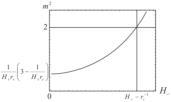
Figure 1: $m^{2}$ as a function of $H_{-}$

Fig. 1 shows that no ghost mode appears if the relation

$$H_{-}>H_{s}:=H_{+}-r_{c}^{-1},$$ (42)

is satisfied. Otherwise, one ghost mode whose mass eigenvalue $m^{2}$ is smaller than 2 appears.

Next we turn to the issue of finding a more explicit form for $\beta$. For this purpose, we solve

$$\left(\hat{L}^{(TT)}+{2\over a^{2}}\right)Q(y)+4r_{c}\sum_{\sigma=\pm}H_{\sigma}^{2}Q(y)\delta(y-y_{\sigma})=-J\delta(y-y_{+}),$$ (43)

in two different ways. First we solve this equation by expanding $Q(y)$ in terms of $u_{i}(y)$ as

$$Q(y)=\sum_{i=0}^{\infty}Q^{(i)}u_{i}(y).$$

Substituting this expansion into the above equation (43) and using the orthonormal conditions of the eigen-functions, we obtain

$$Q(y)=\sum_{i=0}^{\infty}{u_{i}(y_{+})u_{i}(y)\over m_{i}^{2}-2}J.$$

Another way is to solve Eq. (43) more explicitly. The bulk part is solved by

$$Q(y)=C_{0}+C_{1}a(y),$$ (44)

and $C_{0}$ and $C_{1}$ are constants to be determined by the conditions at $y=y_{\pm}$. These conditions are

$$2H_{+}\left(-1+H_{+}r_{c}\right)C_{0}+\left(-1+2H_{+}r_{c}\right)C_{1}=-{1\over 2}J,$$ (45)

$$2H_{-}\left(1+H_{-}r_{c}\right)C_{0}+\left(1+2H_{-}r_{c}\right)C_{1}=0.$$ (46)

Solving these for $C_{0}$ and $C_{1}$, we obtain

$$C_{0}=\frac{-(1+2H_{-}r_{c})}{4H_{+}(H_{+}r_{c}-1)(1+2H_{-}r_{c})-4H_{-}(2H_{+}r_{c}-1)(1+H_{-}r_{c})}J,$$ (47)

$$C_{1}=\frac{H_{-}(1+H_{-}r_{c})}{2H_{+}(H_{+}r_{c}-1)(1+2H_{-}r_{c})-2H_{-}(2H_{+}r_{c}-1)(1+H_{-}r_{c})}J.$$ (48)

Substituting (48) into Eq. (44), we obtain $Q(y)$. Comparing the expressions for $Q(y_{+})$ evaluated in these two different ways, we find

$$\sum_{i=0}^{\infty}{u_{i}^{2}(y_{+})\over m_{i}^{2}-2}={1\over H_{+}}\frac{2H_{-}(1+H_{-}r_{c})-H_{+}(1+2H_{-}r_{c})}{4H_{+}(H_{+}r_{c}-1)(1+2H_{-}r_{c})-4H_{-}(2H_{+}r_{c}-1)(1+H_{-}r_{c})}.$$ (49)

Substituting this into Eq. (33), we finally find

$$\beta = \frac{3H_{+}^{2}(2H_{+}r_{c}-1)}{64\kappa^{2}(1+2H_{-}r_{c})}\left({H_{+}(H_{+}r_{c}-1)(1+2H_{-}r_{c})-H_{-}(2H_{+}r_{c}-1)(1+H_{-}r_{c})}\right)$$ (50)

$$= \frac{3H_{+}^{2}(2H_{+}r_{c}-1)^{2}}{64\kappa^{2}}\left({\hat{H}_{+}(1+\hat{H}_{+}r_{c})\over(1+2\hat{H}_{+}r_{c})}-{H_{-}(1+H_{-}r_{c})\over(1+2H_{-}r_{c})}\right),$$ (51)

where $\hat{H}_{+}:=H_{+}-r_{c}^{-1}$. One can see $\beta$ changes its signature at $H_{-}=\hat{H}_{+}$. When $H_{-}>\hat{H}_{+}$ ($H_{-}<\hat{H}_{+}$), $\beta$ is negative (positive). This means that only when the spin-2 ghost modes are absent, the spin-0 mode becomes a ghost mode. (See Eq. (42).) Consequently, this model always has a ghost.

III Stabilization

In the preceding section, we have seen that when the spin-2 excitations have no ghost, the spin-0 brane-bending excitation becomes a ghost instead. Usually spin-2 excitations (i.e., transverse-traceless tensor modes) are completely decoupled from spin-0 excitations at linear order. However, we can construct a transverse-traceless tensor from a spin-0 mode whose mass squared is $-4H^{2}$. For a scalar function $\Phi$ that satisfies $(\Box^{(4)}+4)\Phi=0$, we can compose a transverse-traceless tensor as

$$\Psi_{\mu\nu}=\left(\nabla_{\mu}\nabla_{\nu}-{1\over 4}\gamma_{\mu\nu}\Box\right)\Phi.$$ (52)

It is trivial to show that this tensor is traceless. The transverse property, $\nabla^{\mu}\Psi_{\mu\nu}=0$, can be shown by using Eq. (17). $\Psi_{\mu\nu}$ is also an eigen-function of $\Box^{(4)}$, but its eigenvalue differs from that of $\Phi$, which is $-4$. By using the identity (27), the mass eigenvalue of the induced spin-2 perturbation $\Psi_{\mu\nu}$ for the operator $(\Box^{(4)}-2)$ is found to be

$$m^{2}=2.$$ (53)

Usually, we identify $H_{\pm}^{2}m^{2}$ as the mass of a rank-two tensor field seen by observers on the $(\pm)$-brane. Hence, the mass squared of this special mode is $2H_{\pm}^{2}$ in the language of spin-2 perturbations. On the other hand, the mass squared of the corresponding spin-0 mode, which is the eigenvalue of $H^{2}\Box^{(4)}$, is $-4H_{\pm}^{2}$. Here, we refer to the mass of this mode as the critical mass. This mass agrees with the threshold mass below which the spin-2 ghost appears. If the mass of a spin-2 mode is smaller than this critical mass, the helicity 0 part of the mode becomes a ghost Higuchi .

In the two-branes model discussed in the preceding section, the unique spin-0 excitation mode has exactly this critical mass. On the other hand, $m^{2}=2$ is the threshold spin-2 mass below which a ghost appears. If we gradually decrease the separation of the two branes, the ghost in spin-2 excitations eventually disappears. The mode that was previously carrying a ghost satisfies $m^{2}=2$ at the critical point. At this point this spin-2 mode can couple with the spin-0 excitations as an exceptional case. After passing the critical point, the ghost is transferred to the spin-0 excitations.

Then, what happens if we introduce a mechanism to stabilize the separation of the branes? Since the mass spectrum of spin-0 excitations changes TM , the spin-0 mode with its mass squared being $-4H^{2}$ will no longer exist. In fact, the smallest mass squared must be large enough if the stabilization mechanism works. Then, again we consider the situation in which the brane separation is gradually decreased. When the spin-2 ghost disappears, we expect absence of the spin-0 mode at the critical mass, which can exceptionally couple to spin-2 excitations. Then there seems to be no reason why the spin-2 ghost is transferred to the spin-0 ghost at the critical point.

However, by studying models stabilized by a bulk scalar field, we will find below that our naive expectation is wrong. What we will see is the following. With a bulk scalar field, there appears an infinite tower of Kaluza-Klein modes for spin-0 excitations. The smallest value of the mass squared of spin-0 excitations is not, in general, equal to $-4H^{2}$ as is expected. However, at the critical point where the smallest mass eigenvalue for spin-2 excitations $m^{2}$ crosses $2$, one of the values of the mass squared of spin-0 excitations also crosses the critical value $-4H^{2}$. As a result, a spin-0 mode whose mass squared is smaller than $-4H^{2}$ arises if the smallest $m^{2}$ is greater than 2, and the spin-0 mode becomes a ghost. We discuss how this happen in detail below.

III.1 Background

We introduce a bulk scalar field to stabilize the brane separation TM . The action is given by

$$S=S_{2}+S_{s},$$ (54)

$$S_{s}:=\int d^{5}x\sqrt{-g}\left(-\frac{1}{2}g^{ab}\psi_{,a}\psi_{,b}-V_{B}(\psi)-\sum_{\sigma=\pm}V^{(\sigma)}(\psi)\delta(y-y_{\sigma})\right).$$ (55)

By choosing the potential in the bulk $V_{B}(\psi)$ and the potentials on the branes $V^{(\sigma)}(\psi)$ appropriately, we can stabilize the brane separation. In the following discussion we do not need the explicit form of the potential functions. The unperturbed background configuration is similar to the previous case. The bulk metric is given by (3) and the branes are located at a fixed value of $y(=y_{\pm})$ as before. But the functional form of the warp factor $a(y)$ is different. The background bulk equations for the warp factor $a(y)$ and the scalar field $\psi$ are

$$\frac{a^{\prime\prime}}{a}-\left(\frac{a^{\prime}}{a}\right)^{2}=-\frac{\kappa^{2}}{3}\psi^{\prime}{}^{2}-\frac{1}{a^{2}},$$ (56)

$$\left(\frac{a^{\prime}}{a}\right)^{2}=\frac{\kappa^{2}}{6}\left(\frac{1}{2}\psi^{\prime}{}^{2}-V_{B}\right)+\frac{1}{a^{2}},$$ (57)

$$\psi^{\prime\prime}+4\frac{a^{\prime}}{a}\psi^{\prime}-{\partial V_{B}\over\partial\psi}=0.$$ (58)

III.2 Perturbations

We use the “Newton gauge”, in which the spin-0 component of the shear of the hypersurface normal vector vanishes, following Ref. TM . In this gauge, using the traceless part and $\{y\mu\}$-component of the Einstein equations, we find that perturbations of the metric and the scalar field are related as

$$h_{yy}=2\phi,\quad h_{y\mu}=0,$$ (59)

$$h_{\mu\nu}=h^{(TT)}_{\mu\nu}-\phi\tilde{\gamma}_{\mu\nu},$$ (60)

$$\delta\psi=\frac{3}{2\kappa^{2}\psi^{\prime}}\left[\partial_{y}+2{\cal H}\right]\phi,$$ (61)

where $\tilde{\gamma}_{\mu\nu}:=a^{2}(y)\gamma_{\mu\nu}$, ${\cal H}:=a^{\prime}/a$ and $h_{\mu\nu}^{(TT)}$ is a tensor which satisfies transverse-traceless conditions. Here, one remark is in order. For modes at the critical mass there is a possible coupling between spin-0 and spin-2 excitations. Recall that the traceless tensor generated by acting a derivative operator from a scalar-type function ($[\nabla_{\mu}\nabla_{\nu}-\frac{1}{4}\gamma_{\mu\nu}\Box^{(4)}]\Phi$ ) is automatically transverse. Due to this mixing, vanishing of spin-0 component of the shear is slightly ambiguous. Here we define the “Newton gauge” by the above form of perturbations (61), and therefore it actually can possess spin-0 component of the shear for the mode with this critical eigenvalue. In this sense, the gauge is not completely fixed.

In the present gauge, the bulk equations for $h^{(TT)}_{\mu\nu}$ become

$$\left[\hat{L}^{(TT)}+\frac{1}{a^{2}}(\Box^{(4)}\!-2)\right]h^{(TT)}_{\mu\nu}=0,$$ (62)

with $h^{(TT)}$ as defined in (15). While, the bulk equation for $\phi$ becomes

$$\left[\hat{L}^{(\phi)}+{1\over\psi^{\prime}{}^{2}}(\Box^{(4)}\!+4)\right]\phi=0,$$ (63)

with

$$\hat{L}^{(\phi)}:=a^{2}\partial_{y}\frac{1}{a^{2}\psi^{\prime}{}^{2}}\partial_{y}a^{2}-\frac{2\kappa^{2}}{3}a^{2}.$$ (64)

We first write down the junction conditions to impose at the branes in the “Gaussian normal” coordinates. Perturbation variables with an over-bar “$~{}\bar{}~{}$” are understood as those in the “Gaussian normal” coordinates, as before. The junction conditions for metric perturbations are

$$\pm\left(\partial_{\bar{y}}-2{\cal H}\right)\bar{h}^{(\pm)}_{\mu\nu}=-\kappa^{2}\left[T^{(\pm)}_{\mu\nu}-\frac{1}{3}\tilde{\gamma}_{\mu\nu}T^{(\pm)}\right]\mp\frac{2\kappa^{2}}{3}\tilde{\gamma}_{\mu\nu}\psi^{\prime}\delta\psi+2r_{c}\left[X_{\mu\nu}-{1\over 3}\tilde{\gamma}_{\mu\nu}X\right],$$ (65)

with $X_{\mu\nu}$ defined in (10). While, the condition for the bulk scalar field is

$$\pm 2\delta{\bar{\psi}^{\prime}}=V^{\prime\prime(\pm)}(\psi)\delta\bar{\psi}.$$ (66)

The generators of the gauge transformation from the “Gaussian normal” coordinates to the Newton gauge take the form of

$$\xi^{y}_{(\pm)}=\int^{y}\phi(y^{\prime})dy^{\prime}=\int_{y_{\pm}}^{y}\phi(y^{\prime})dy^{\prime}+\hat{\xi}^{y}_{(\pm)}(x^{\mu}),$$ (67)

$$\xi_{(\pm)}^{\nu}=-\int^{y}\tilde{\gamma}^{\mu\nu}(y^{\prime})dy^{\prime}\int^{y^{\prime}}\phi_{,\mu}(y^{\prime\prime})dy^{\prime\prime}$$

$$\qquad=-\int^{y}_{y_{\pm}}\tilde{\gamma}^{\mu\nu}(y^{\prime})\left[\int_{y_{\pm}}^{y^{\prime}}\phi_{,\mu}(y^{\prime\prime})dy^{\prime\prime}+\hat{\xi}^{y}_{(\pm),\mu}(x^{\rho})\right]dy^{\prime}+\hat{\xi}^{\nu}_{(\pm)}(x^{\rho}).$$ (68)

Under this gauge transformation, the perturbation variables transform as

$$\bar{h}^{(\pm)}_{\mu\nu}(y)=h_{\mu\nu}(y)+2\nabla{}_{(\mu}\xi{}_{\nu)}{}^{\!\!\!\!\!\!(\pm)}-2{\cal H}\tilde{\gamma}_{\mu\nu}(y)\xi^{y}_{(\pm)},$$ (69)

$$\delta\bar{\psi}^{\pm}(y)=\delta\psi(y)-\psi^{\prime}\xi^{y}_{(\pm)}+\hat{\xi}^{y}_{(\pm)}.$$ (70)

Substituting these relations into Eqs. (65) and (66), we obtain the junction conditions in the Newtonian gauge. The conditions for the traceless part of metric perturbations become

$$\pm\left(\partial_{y}-2{\cal H}_{\pm}\right)h^{(TT)}_{\mu\nu}=-\kappa^{2}\Sigma_{\mu\nu}^{(\pm)}-r_{c}H_{\pm}^{2}({\Box^{(4)}\!-2})h^{(TT)}_{\mu\nu},$$ (71)

with ${\cal H}_{\pm}:={\cal H}(y_{\pm})$ and

$$\Sigma^{(\pm)}_{\mu\nu}:=\left(T^{(\pm)}_{\mu\nu}-\frac{1}{4}T^{(\pm)}\tilde{\gamma}_{\mu\nu}\right)\pm\frac{2}{\kappa^{2}}\left(\nabla_{\mu}\nabla_{\nu}-\frac{1}{4}\gamma_{\mu\nu}\Box^{(4)}\right)Z_{(\pm)}.$$ (72)

On the other hand, the condition for the trace part of metric perturbations becomes

$$H_{\pm}^{2}({\Box^{(4)}\!+4})Z_{(\pm)}=\pm\frac{\kappa^{2}}{6}T^{(\pm)},$$ (73)

where

$$Z_{(\pm)}=\left(1\mp 2r_{c}{\cal H}_{\pm}\right)\hat{\xi}_{(\pm)}^{y}-r_{c}\phi(y_{\pm}).$$ (74)

The junction condition for the scalar-type perturbation becomes

$$\pm\frac{2\kappa^{2}}{3}\left(\delta\psi-\psi^{\prime}\left(1\mp 2r_{c}{\cal H}\right)^{-1}(Z_{(\pm)}+r_{c}\phi)\right)=\frac{\epsilon^{(\pm)}}{a^{2}\psi^{\prime}}\left(\Box^{(4)}\!+4\right)\phi,$$ (75)

at $y=y_{\pm}$ with

$$\epsilon^{(\pm)}:=\frac{2}{V^{\prime\prime(\pm)}\pm 2\psi^{\prime\prime}/\psi^{\prime}}\quad.$$ (76)

In the following discussion we assume $\epsilon^{(\pm)}\geq 0$, which includes the simplest case of the tight binding limit; $V^{\prime\prime}{}^{(\pm)}\to\infty$.

Combining the bulk equations and the junction conditions, we formally obtain the same equation as (14) for spin-2 excitations, and

$$\left[\hat{L}^{(\phi)}+{1\over\psi^{\prime}{}^{2}}(\Box^{(4)}\!+4)\right]\phi=\sum_{\sigma=\pm}\left(\sigma\frac{4a^{2}\kappa^{2}}{3}\left(1-\sigma 2r_{c}{\cal H}_{\pm}\right)^{-1}(Z_{(\sigma)}+r_{c}\phi)-{2\epsilon^{(\sigma)}\over\psi^{\prime}{}^{2}}(\Box^{(4)}\!+4)\phi\right)\delta(y-y_{\sigma}),$$ (77)

for spin-0 excitations.

III.3 Solution with source

As was done in §II, we formally write down a solution of perturbation equations for a given energy momentum tensor by using the Green’s function written in terms of eigen-functions of $\hat{L}^{(TT)}$ and $\hat{L}^{(\phi)}$. We also derive expressions for the metric perturbations induced on the branes.

We begin with spin-2 excitations. We expand the metric perturbation $h_{\mu\nu}^{(TT)}$ by using the eigen-functions of the eigenvalue problem (18), as before. The calculation closely parallels the previous case, although the functional form of the warp factor $a$ is not the same. We obtain (23), formally the same expression as before.

Spin-0 excitations can be solved in the same way. We define the eigen-functions $v_{i}(y)$ by

$$\frac{\mu_{i}^{2}+4}{\psi^{\prime}{}^{2}}\left(1+\sum_{\sigma=\pm}2\epsilon^{\sigma}\delta(y-y_{\sigma})\right)v_{i}(y)=\left[-\hat{L}^{(\phi)}+\sum_{\sigma=\pm}\sigma{4r_{c}\kappa^{2}a^{2}\over 3}\left(1-\sigma 2r_{c}{\cal H}_{\pm}\right)^{-1}\delta(y-y_{\sigma})\right]v_{i}(y),$$ (78)

and we define the inner product by

$$(v_{i},v_{j})^{(\phi)}:=\oint\frac{dy}{\psi^{\prime}{}^{2}}\left(1+\sum_{\sigma=\pm}2\epsilon^{\sigma}\delta(y-y_{\sigma})\right)v_{i}(y)v_{j}(y).$$ (79)

Under the assumption that $\epsilon^{\sigma}\geq 0$, it is trivial to show that the norm of each eigenfunction is positive definite, and hence they can be normalized as $(v_{i},v_{j})^{(\phi)}=\delta_{ij}$. Using thus normalized eigen-functions, the solution of Eq. (77) is given by

$$\phi(y)=\frac{4\kappa^{2}}{3H_{+}^{2}}\left(1-2r_{c}{\cal H_{+}}\right)^{-1}\sum_{i}{v_{i}(y_{+})v_{i}(y)\over\Box^{(4)}\!-\mu_{i}^{2}}Z_{(+)}.$$ (80)

The induced metric on the brane for the solution with the source is given by

$$\bar{h}_{\mu\nu}^{(+)} = h_{\mu\nu}^{(TT)}(y_{+})-\tilde{\gamma}_{\mu\nu}\left(\phi(y_{+})+2{\cal H}_{+}\hat{\xi}^{y}_{(+)}\right),$$ (81)

Here, transverse-traceless part $h_{\mu\nu}^{(TT)}$ takes the same form as given in Eq. (23), and it can be rewritten more explicitly as

$$h_{\mu\nu}^{(TT)}(y_{+}) = -2\kappa^{2}\sum_{i}{u_{i}^{2}(y_{+})\over\Box^{(4)}-2-m_{i}^{2}}\left(T_{\mu\nu}^{(+)}-{1\over 4}\tilde{\gamma}_{\mu\nu}T^{(+)}+{H_{+}^{-2}\over 3(m_{i}^{2}-2)}\left(\nabla_{\mu}\nabla_{\nu}-{1\over 4}\gamma_{\mu\nu}\Box^{(4)}\right)T^{(+)}\right)$$ (83)

$$+\frac{2\kappa^{2}}{3H_{+}^{2}}\left(\sum_{i}\frac{u^{2}_{i}(y_{+})}{m_{i}^{2}-2}\right)\left(\nabla_{\mu}\nabla_{\nu}-\frac{1}{4}\gamma_{\mu\nu}\Box^{(4)}\right)\frac{1}{\Box^{(4)}+4}T^{(+)}.$$

While the trace part is computed as

$$\phi+2{\cal H}_{+}\hat{\xi}^{y}_{(+)} = {2\kappa^{2}\over 9\tilde{H}_{+}^{4}}\sum_{i}{v_{i}^{2}(y_{+})\over\mu_{i}^{2}+4}{1\over\Box^{(4)}-\mu_{i}^{2}}T^{(+)}$$ (85)

$$-{\kappa^{2}\over 3\tilde{H}_{+}^{2}}\left({2\kappa^{2}\over 3\tilde{H}_{+}^{2}}\left(\sum_{i}{v_{i}^{2}(y_{+})\over\mu_{i}^{2}+4}\right)+{a^{\prime}\over a}\right){1\over\Box^{(4)}+4}T^{(+)},$$

where for brevity we have introduced

$$\tilde{H}_{+}^{2}=H_{+}^{2}\left(2r_{c}{\cal H}_{+}-1\right).$$ (86)

The above expression for $\bar{h}_{\mu\nu}^{(+)}$ apparently contains a pole at the critical mass eigenvalue corresponding to $(\Box^{(4)}+4)^{-1}$. The term proportional to $\nabla_{\mu}\nabla_{\nu}$ in Eq. (83) is pure gauge. Hence, the contribution from the pole at the critical mass eigenvalue is proportional to $\gamma_{\mu\nu}(\Box^{(4)}+4)^{-1}T^{(+)}$. Collecting such terms in $\bar{h}_{\mu\nu}^{(+)}$ coming both from the $TT$-part and from the scalar-part, the coefficient becomes

$${\kappa^{2}\over 3H_{+}^{2}}\left\{2\left(\sum_{i}{u_{i}^{2}(y_{+})\over m_{i}^{2}-2}\right)+{1\over\tilde{H}_{+}^{2}}\left({2\kappa^{2}\over 3\tilde{H}_{+}^{2}}\left(\sum_{i}{v_{i}^{2}(y_{+})\over\mu_{i}^{2}+4}\right)+{\cal H}_{+}\right)\right\}.$$ (87)

In §III.4 we will prove an identity which shows that this coefficient vanishes as a whole.

III.4 No physical degrees of freedom at critical mass

As we mentioned earlier, our “Newton gauge” is not a complete gauge fixing. In this section, we will fist show that there is no physical mode at the critical mass in general after completely fixing the residual gauge. Next, we will show that the value of the expression (87) equals $0$.

The residual gauge degree of freedom of our “Newton gauge” exists at the critical mass, i.e., when $\Box^{(4)}\!=-4$ for scalar-type perturbations and $\Box^{(4)}\!=4$ for transverse-traceless tensor perturbations. To see this, let’s consider the gauge transformation generated by the following infinitesimal coordinate transformation:

$$\xi^{y}={1\over 2}a^{2}\partial_{y}\left({X\over a^{2}}\right),\qquad\xi^{\mu}=-{1\over 2}\tilde{\gamma}^{\mu\nu}X_{,\nu}.$$ (88)

This gauge transformation keeps the conditions $h_{y\mu}=0$. The change of $\phi$ induced by this gauge transformation can be read off the $\{yy\}$-component of the metric perturbation:

$$\delta\phi={1\over 2}\partial_{y}\left(a^{2}\partial_{y}\left({X\over a^{2}}\right)\right).$$ (89)

At the same time, the induced change of $\phi$ can be also read off the trace part of the metric perturbation:

$$\delta\phi=-a^{\prime}a\,\partial_{y}\left({X\over a^{2}}\right)-{X\over a^{2}},$$ (90)

where we have used $\Box^{(4)}X=-4X$. Equating these two expressions, we obtain an equation for $X$, which is

$$\hat{L}^{(TT)}X=-{2\over a^{2}}X.$$ (91)

Gauge transformations with $X$ satisfying this equation preserve the “Newton gauge” conditions. Hence, such gauge transformations represent the residual gauge degrees of freedom.

Notice that the above equations are identical to the equations for the $TT$-part (18) with $\Box^{(4)}\!=4$. The traceless part generated by this gauge transformation is

$$\delta h^{(TT)}_{\mu\nu}=-\left(\nabla_{\mu}\nabla_{\nu}-{1\over 4}\gamma_{\mu\nu}\Box^{(4)}\right)X.$$ (92)

Therefore, Eq. (91) means that the $h^{(TT)}_{\mu\nu}$ induced by the residual gauge transformation satisfies the perturbation equation consistently. It is also straight forward to show that $\phi=\delta\phi$ given by Eq. (89), or equivalently by Eq. (90), satisfies the equation for the scalar-type perturbation with $\Box^{(4)}\!=-4$. To conclude, solutions of the bulk perturbation equations for both spin-2 and spin-0 parts at the critical mass are generated by a gauge transformation.

Next, we turn to the the issue of boundary conditions. As we are interested in the gravitational degrees of freedom, we consider cases without matter fields: $T^{(\pm)}=0$. From Eq. (73), we find $(\Box^{(4)}+4)Z_{(\pm)}=0$. Both spin-2 and spin-0 parts are sourced by $Z_{(\pm)}$ and they have solutions for any given $Z_{(\pm)}$. However, the spin-2 part of the solution, which is proportional to $\left(\nabla_{\mu}\nabla_{\nu}-{1\over 4}\gamma_{\mu\nu}\Box^{(4)}\right)Z_{(\pm)}$, can be erased by the residual gauge transformation mentioned above. By the definition of residual gauge transformation, it does not violate the gauge conditions necessary to derive the set of perturbation equations (14) and (77). Therefore the solution after this gauge transformation still satisfies all the perturbation equations. Once the $TT$-part is completely erased by the gauge transformation, the junction conditions therefore imply that $Z_{(\pm)}$ also vanishes after this gauge transformation. The equation of motion for the scalar part also continues to hold after the gauge transformation. But now, with vanishing $Z_{(\pm)}$, the only consistent solution for $\phi$ is $\phi\equiv 0$, except for models with the potentials $V_{B}$ and $V^{(\pm)}$ being fine tuned.

For any given homogeneous solution of $Z_{(\pm)}$, we can construct a solution for the bulk perturbations which solves all the perturbation equations. However, what we have found is that seemingly non-trivial solutions constructed in such a manner are all pure gauge modes related to the residual gauge degrees of freedom of the “Newton gauge”. As we have anticipated, there is no physical perturbation mode at the critical mass.

We found that by fixing the residual gauge, we can set $Z_{(\pm)}=0$ in the source-free case, and therefore we succeeded in eliminating the mode at the critical mass from the physical spectrum. Using this fact, we can prove that the expression presented in (87) vanishes as follows: By making a residual gauge transformation to the unperturbed background, we can set $Z_{(+)}=Z_{0}$ for such $Z_{0}$ that satisfies $(\Box^{(4)}+4)Z_{0}=0$. After the gauge transformation, we obtain a pure gauge mode for $h^{(TT)}_{\mu\nu}$ and $\phi$ at the critical mass. From Eqs. (90) and (92), this gauge mode is given explicitly by

$$h^{(TT)}_{c\,\mu\nu}=-\left(\nabla_{\mu}\nabla_{\nu}-{1\over 4}\gamma_{\mu\nu}\Box^{(4)}\right)X,$$ (93)

$$\phi_{c}=-a^{\prime}a\,\partial_{y}\left({X\over a^{2}}\right)-{X\over a^{2}},$$ (94)

where a subscript $c$ indicates the mode at the critical mass. Since it is a pure gauge mode, the above mode should satisfy the junction conditions (75) and (71) with $Z_{(+)}=Z_{0}$ and $T^{(\pm)}_{\mu\nu}=0$. Both conditions give the same boundary condition for $X$. Substituting (93) into (71) at $y=y_{+}$, we obtain

$$\left.a^{2}\partial_{y}\left(\frac{X}{a^{2}}\right)\right|_{y=y+}=2Z_{0}-\left.2r_{c}H_{+}^{2}{X}\right|_{y=y+}.$$ (95)

Substituting this into Eq. (94) to eliminate $\partial_{y}X$, we get

$$\phi_{c}(y_{+})=-2{\cal H}_{+}Z_{0}-H_{+}^{2}\left(1-2r_{c}{\cal H}_{+}\right)X.$$ (96)

On the other hand, from Eqs. (23) and (80) with the aid of (93), we have

$$X=4\sum_{i}\frac{u_{i}^{2}(y_{+})}{2-m_{i}^{2}}Z_{0},\qquad\mbox{and}\qquad\phi_{c}=\frac{4\kappa^{2}}{3\tilde{H}^{2}_{+}}\sum_{i}\frac{v^{2}_{i}(y_{+})}{4+\mu^{2}_{i}}Z_{0}.$$ (97)

Combining Eqs. (96) and (97), we finally obtain

$$2\left(\sum_{i}{u_{i}^{2}(y_{+})\over m_{i}^{2}-2}\right)+{1\over\tilde{H}_{+}^{2}}\left({2\kappa^{2}\over 3\tilde{H}_{+}^{2}}\left(\sum_{i}{v_{i}^{2}(y_{+})\over\mu_{i}^{2}+4}\right)+{\cal H}_{+}\right)=0.$$ (98)

Namely, the coefficient of the pole at the critical mass, (87), vanishes.

Although Eqs. (83) and (85) apparently contain poles at the critical mass, we find that they completely cancel each other. This is consistent with the conclusion obtained earlier in this subsection that there is no physical mode at the critical mass.

III.5 Effective action and ghost conditions

Applying the same method used in §II.4, we now derive the four dimensional effective action to the quadratic order for the present case. From the derived effective action, we will identify the conditions for the presence of ghost.

We denote the Kaluza-Klein towers of the transverse-traceless part and the trace part of the metric perturbation induced on the $(+)$-brane by $\bar{h}^{(i)}_{\mu\nu}$ and $\bar{h}^{(j)}$, respectively. The induced metric perturbation is given by

$$\bar{h}_{\mu\nu}=\sum_{i}\bar{h}^{(i)}_{\mu\nu}+{1\over 4}\tilde{\gamma}_{\mu\nu}\sum_{j}\bar{h}^{(j)}.$$

Then, the kinetic term of the effective action is

$$S_{kin} = \sum_{i}\alpha_{i}\int d^{4}x\sqrt{-g}\,\bar{h}^{(i)\mu\nu}(\Box-2-m_{i}^{2})\bar{h}_{\mu\nu}^{(i)}$$ (100)

$$\qquad+\sum_{j}\beta_{j}\int d^{4}x\sqrt{-g}\,\bar{h}^{(j)}(\Box-\mu_{j}^{2})\bar{h}^{(j)},$$

and the action of the matter localized on the $(+)$-brane is

$$S^{(+)}_{matter}=(\mbox{0-th order of }\bar{\bf h}) \!\!+\!\! \sum_{i}\frac{1}{2}\int d^{4}x\sqrt{-g}T_{(+)}^{\mu\nu}\bar{h}_{\mu\nu}^{(i)}$$ (101)

$$\!\!+\!\! \sum_{j}{1\over 8}\int d^{4}x\sqrt{-g}T^{(+)}\bar{h}^{(j)}+O(\bar{\bf h}^{2}).$$

Comparing the equations of motion derived from the variation of $S_{kin}+S_{matter}$ with Eqs. (83) and (85), we find

$$\alpha_{i}={1\over 8\kappa^{2}u_{i}^{2}(y_{+})},\qquad\beta_{j}={9\tilde{H}_{+}^{4}(\mu^{2}_{i}+4)\over 128\kappa^{2}v_{i}^{2}(y_{+})}.$$ (102)

All coefficients of the spin-2 component, $\alpha_{i}$, are always positive. However, when the mass eigenvalue is in the range $0<m^{2}_{i}<2$, such a mode contains a ghost in its helicity zero component. In contrast, the coefficients of spin-0 component, $\beta_{i}$, becomes negative when $\mu_{i}^{2}<-4$. In this case this mode becomes a ghost. Hence, to realize a ghost-free model, all masses of spin-2 modes and spin-0 modes must satisfy $m^{2}_{i}>2$ and $\mu_{i}^{2}>-4$. However, it turns out to be impossible that both conditions are satisfied simultaneously.

In order to show this, we consider continuous deformation of the model potentials of the bulk scalar field. When the smallest eigenvalue of spin-2 excitations, $m^{2}_{0}$, approaches 2 from below, ${u_{0}^{2}(y_{+})/(m^{2}_{0}-2)}$ in Eq. (98) diverges. Since this equality is always satisfied, this divergence must be compensated by the other terms. The possibility is that one of the eigenvalues of spin-0 excitations $\mu_{j}^{2}$ approaches $-4$ from above. Therefore, when the value of $m^{2}_{0}$ exceeds 2, at least one of the values, $\mu^{2}_{j}$, must be smaller than $-4$. Hence, we cannot simultaneously satisfy $m_{0}^{2}>2$ and $\mu_{0}^{2}>-4$ by a continuous deformation. All models specified by given bulk scalar field potentials are connected with each other by continuous deformations. Thus it is proved that we cannot realize a model free from a ghost within the two-brane extension of the DGP model with a bulk scalar field.

In the above discussion we have introduced the four dimensional effective action just from the notion of the equations of motion. Homogeneous equations of motion are sufficient to fix the form of the effective action except for the overall normalization of each mode. However, to determine if there is a ghost or not, the overall normalization is crucial . We have determined this overall normalization factor by investigating the coupling to the matter energy momentum tensor.

There are alternative ways to fix this overall normalization for each mode without looking at the coupling to matter fields. We could have derived a four dimensional effective action directly from the original five dimensional action, although we feel that the approach adopted in this paper is slightly easier. One short cut to fix this normalization is just to look at the bulk part of the five dimensional reduced action written down in terms of the master variable. To obtain the five dimensional action, we can use double Wick rotation: $y\to iy$ and $t\to-it$, which transforms the four dimensional de Sitter space into an Euclidean four sphere. Then, the discussion in the bulk is completely parallel to the cosmological perturbation in the (five dimensional) closed FRW universe, and we can make use of the knowledge about the effective action in the context of the cosmological perturbation in the FRW universeopen . Since our action should be obtained by the double Wick rotation from this action, one can easily read the correct form of the reduced action including the overall normalization. By doing so, we will find that when and only when $\mu^{2}_{i}<-4$, the overall normalization factor becomes negative for spin-0 excitations. For spin-2 excitations, the overall factor is always positive definite. This gives an another route to reach the same conclusion that we have obtained in this section.

IV Summary

In the present paper, we have attempted to construct a ghost-free model by modifying the self-accelerating branch of the DGP brane world scenario, in which the spin-2 sector drives the accelerated expansion of the universe. We first tried adding an additional boundary brane in §II, and then stabilizing the brane separation by introducing a bulk scalar field in §III. In both cases, we found that the ghost excitation survives. As we have already mentioned in Introduction, this is caused by the degeneracy between spin-2 and spin-0 modes at the critical mass. This degeneracy enables the ghost property to transmute between these two normally decoupled modes. But this degeneracy occurs only at this special mass.

In the case without stabilization, the fluctuation of brane separation gives the spin-0 mode. Hence, if we fix the brane separation, the mass spectrum of spin-0 excitations will be significantly modified. We introduced Goldberger-Wise mechanism GW into our two-branes model. Then, in general the spin-0 spectrum does not have a mode at the critical mass. However, when the spin-2 mode crosses the critical mass, we found that the one of the mass of spin-0 mode also crosses the critical value, and it turns into a ghost. We have explained why we cannot avoid this exchange of a ghost degree of freedom in detail in the text. The point is as follows: If we compute the effective action for the matter field obtained after integrating out the gravitational degrees of freedom, the spin-2 contribution unexpectedly gives the term depending on the trace of the matter energy momentum tensor. This is because the spin-2 perturbation is sourced by the brane bending, which is sourced by the trace of the energy momentum tensor. Although this brane bending does not appear in the physical spectrum of the model once stabilization is introduced, its mass still corresponds to the critical mass. As a result, when one of the masses of the spin-2 excitations crosses the critical value, the pole of the brane bending resonates with the pole of this crossing mode. This leads to the divergence of the effective action of the matter field. Physically, however, any divergence in the effective action is not expected. This divergence is cancelled by the contribution from the spin-0 mode. But such cancellation is possible only if the mass spectrum of spin-0 modes also crosses the critical mass at the same time.

It is instructive to emphasize the difference of the behaviour of spin-2 perturbations in the DGP model compared to the massive Fierz-Pauli model. In the massive Fierz-Pauli model, a pathology appears if the mass becomes $2H^{2}$ because the equation of motion implies that $T=0$. In the DGP brane world, matter sources need not satisfy $T-0$. Indeed, the solution for transverse-traceless perturbations shows no pathology at $m_{i}^{2}=2$. A pathological behaviour near $m_{i}^{2}=2$ in the spin-2 sector appears because we separated the spin-0 contribution from the spin-2 contribution. This is due to the degeneracy between spin-2 and spin-0 perturbations at $m^{2}=2$, which is explained at the beginning of §III. This means that the DGP model has a natural mechanism to cure the pathology of the massive gravity theory at $m^{2}=2$ with $T\neq 0$ by accommodating the physical spin-0 perturbation at $m^{2}=2$ when the mass of spin-2 perturbations crosses $m^{2}=2$. However, we have shown that it is this mechanism that transfers the ghost between spin-2 and spin-0 modes.

To conclude, we confirmed in this paper that it is really difficult to erase this ghost within the context of standard linear analysis. However, a different way to avoid appearance of ghost is proposed in Ref. Deffayet . We think still further study is necessary to conclude whether this ghost is really harmful or not.

Appendix A Effective action for spin-2 field

A.1 Exact Lagrangian

To obtain the quadratic action for a massive spin-2 field, the method with the surest footing involves starting with the Einstein-Hilbert action with cosmological constant and Fierz-Pauli mass terms. The Lagrangian up to quadratic order on de Sitter background is Higuchi

$$L_{h}=\alpha\sqrt{-\gamma}\biggl{(}-{1\over 4}\nabla_{\mu}h_{\nu\lambda}\nabla^{\mu}h^{\nu\lambda}+{1\over 2}\nabla_{\mu}h^{\mu\lambda}\nabla^{\nu}h_{\nu\lambda}+{1\over 4}\left(\nabla^{\mu}h-2\nabla_{\nu}h^{\mu\nu}\right)\nabla_{\mu}h$$

$$\qquad\qquad\qquad\qquad\qquad\qquad\qquad\qquad\qquad-{1\over 2}\left(h_{\mu\nu}h^{\mu\nu}+{1\over 2}h^{2}\right)-{m^{2}\over 4}\left(h_{\mu\nu}h^{\mu\nu}-h^{2}\right)\biggr{)}.$$ (103)

Here the Hubble parameter is set to unity for simplicity. The overall normalization of the Lagrangian $\alpha$ can be different from the conventional one. (By redefinition of field, one can say that the coupling with the matter energy momentum tensor is unconventional.) The Lagrangian including coupling to the matter will be given by

$$L=L_{h}+L_{m},$$ (104)

with

$$L_{m}={1\over 2}\sqrt{-\gamma}\,h_{\mu\nu}T^{\mu\nu}.$$ (105)

Equations of motion derived from the variation of this Lagrangian become

$$\alpha\left(X_{\mu\nu}-{m^{2}\over 2}\left(h_{\mu\nu}-\gamma_{\mu\nu}h\right)\right)+{1\over 2}T_{\mu\nu}=0,$$ (106)

with

$$X_{\mu\nu}\equiv{1\over 2}\left(\Box h_{\mu\nu}-\nabla_{\mu}\nabla^{\alpha}h_{\alpha\nu}-\nabla_{\nu}\nabla^{\alpha}h_{\alpha\mu}+\nabla_{\mu}\nabla_{\nu}h\right)$$

$$\qquad\qquad\qquad\qquad\qquad\qquad+{1\over 2}\gamma_{\mu\nu}\left(\nabla_{\alpha}\nabla_{\beta}h^{\alpha\beta}-\Box h\right)-\left(h_{\mu\nu}+{1\over 2}\gamma_{\mu\nu}h\right).$$ (107)

Since $\nabla^{\mu}X_{\mu\nu}=0$ and $\nabla^{\mu}T_{\mu\nu}=0$, we have a constraint:

$$\nabla^{\mu}h_{\mu\nu}=\nabla_{\nu}h.$$ (108)

Substituting back this relation to the trace of Eq. (106), we obtain

$$h=-{1\over 3\alpha(m^{2}-2)}T.$$ (109)

Again, substituting the above constraint equations (108) and (109) into Eq. (106), we obtain

$$\alpha(\Box^{(4)}-2-m^{2})h_{\mu\nu} \!\!\!\!=\!\!\!\! -T_{\mu\nu}-{1\over 3(m^{2}-2)}\left(\nabla_{\mu}\nabla_{\nu}-(m^{2}-1)\gamma_{\mu\nu}\right)T$$ (110)

$$\!\!\!\!=\!\!\!\! -\left(T_{\mu\nu}-{1\over 4}\gamma_{\mu\nu}T+{1\over 3(m^{2}-2)}\left(\nabla_{\mu}\nabla_{\nu}-{1\over 4}\gamma_{\mu\nu}\Box^{(4)}\right)T\right)-{\Box^{(4)}-2-m^{2}\over 12(m^{2}-2)}\gamma_{\mu\nu}T.$$ (111)

In the last line, we divided the traceless part and the pure trace part. Comparing the solution of the above equations of motion with the result obtained from the original theory (83), we can read the value of $\alpha$. The contribution of the last term in (111) is combined with the second term in Eq. (83) to obtain

$$\frac{2\kappa^{2}}{3H_{+}^{2}}\left(\sum_{i}\frac{u^{2}_{i}(y_{+})}{m_{i}^{2}-2}\right)\left[\nabla_{\mu}\nabla_{\nu}+\gamma_{\mu\nu}\right]\frac{1}{\Box^{(4)}+4}T^{(+)}.$$ (112)

The first term in the square brackets is pure gauge, while the second term is cancelled by the pole at $(\Box^{(4)}+4)=0$ in the trace part given in (85) as was shown in §III.4.

A.2 Simplified Lagrangian

One may feel like to use the following simplified form of the effective Lagrangian with the constraints (108) and (109) manifestly imposed by using Lagrange multipliers $\lambda_{\mu}$ and $\bar{\lambda}$:

$$L^{\prime}_{h} \!\!\!\!=\!\!\!\! \int d^{4}x\sqrt{-\gamma}\Biggl{(}{\alpha\over 4}\sum_{i}h^{\mu\nu}(\Box^{(4)}-2-m^{2})h_{\mu\nu}$$ (114)

$$\qquad\qquad\qquad\qquad+\left(\nabla_{\nu}h^{\mu\nu}+\nabla^{\mu}{1\over 3\alpha(m^{2}-2))}T\right)\lambda_{\mu}+\left(h^{\mu}_{\ \mu}+{1\over 3\alpha(m^{2}-2))}T\right)\bar{\lambda}\Biggr{)}.$$

This Lagrangian is not completely equivalent to $L_{h}$ as is shown below. Further disadvantage of this Lagrangian is the appearance of $T^{\mu\nu}$ in the gravitational part of the Lagrangian.

Equations of motion derived from the variation of $L^{\prime}_{h}+L_{m}$ are

$${\alpha\over 2}(\Box^{(4)}-2-m^{2})h_{\mu\nu}+{1\over 2}T_{\mu\nu}-\lambda_{(\mu;\nu)}+\gamma_{\mu\nu}\bar{\lambda}=0,$$ (115)

$$\nabla^{\nu}h_{\mu\nu}=-\nabla_{\mu}{1\over 3\alpha(m^{2}-2))}T,$$ (116)

$$h=-{1\over 3\alpha(m^{2}-2))}T.$$ (117)

Trace of Eq. (115) with the aid of Eq. (117) gives

$$-{\Box^{(4)}-2-m^{2}\over 6(m^{2}-2)}T+{1\over 2}T-\nabla_{\mu}\lambda^{\mu}+4\bar{\lambda}=0.$$ (118)

While divergence of Eq. (115) becomes

$$-\nabla_{\mu}{\Box^{(4)}+4-m^{2}\over 6(m^{2}-2)}T-{1\over 2}\left(\Box^{(4)}\lambda_{\mu}+\nabla_{\nu}\nabla_{\mu}\lambda^{\nu}\right)+\nabla_{\mu}\bar{\lambda}=0,$$ (119)

where we have used the equation

$$\nabla^{\mu}\Box^{(4)}h_{\mu\nu} = (\Box^{(4)}+5)\nabla^{\mu}h_{\mu\nu}-2\nabla_{\nu}h$$ (120)

$$= -(\Box^{(4)}+3)\nabla_{\nu}{1\over 3\alpha(m^{2}-2)}T$$

$$= -\nabla_{\nu}(\Box^{(4)}+6){1\over 3\alpha(m^{2}-2)}T.$$

Eliminating $\nabla_{\mu}\bar{\lambda}$ from the gradient of Eq. (118) and Eq. (119), we obtain

$${1\over 2}{1\over(m^{2}-2)}\nabla_{\mu}(\Box^{(4)}+4)T-\nabla_{\mu}\nabla_{\nu}\lambda^{\nu}+2\Box^{(4)}\lambda_{\mu}+2\nabla_{\nu}\nabla_{\mu}\lambda^{\nu}=0.$$ (121)

Divergence of the above equation becomes

$${1\over 2}{1\over(m^{2}-2)}\Box^{(4)}(\Box^{(4)}+4)T-3(\Box^{(4)}+4)\nabla_{\mu}\lambda^{\mu}=0,$$ (122)

where we have used

$$\nabla^{\mu}\Box^{(4)}\lambda_{\mu} = \nabla^{\mu}\nabla_{\nu}\nabla_{\mu}\lambda^{\nu}$$ (123)

$$= (\Box^{(4)}+3)\nabla_{\mu}\lambda^{\mu}.$$

If we neglect the possibility of adding an arbitrary solution of the homogeneous equation $(\Box^{(4)}+4)\nabla_{\mu}\lambda^{\mu}=0$, we find

$$\nabla_{\mu}\lambda^{\mu}=-{\Box^{(4)}\over 6(m^{2}-2)}T.$$ (124)

Substituting this equation into Eq. (118), we find

$$\bar{\lambda}=-\frac{m^{2}-1}{6(m^{2}-2)}T.$$ (125)

Substitution of this equation and Eq. (124) back into Eq. (119) results in

$$(\Box^{(4)}+3)\lambda_{\mu}=-{(\Box^{(4)}+3)\over 6(m^{2}-2)}\nabla_{\mu}T.$$ (126)

Again, if we neglect the homogeneous solution, we find

$$\lambda_{\mu}=-{1\over 6(m^{2}-2)}\nabla_{\mu}T.$$ (127)

If we substitute (125) and (127) into (115), we obatain the same equation as Eq. (111). However, strictly speaking, this system has propagating modes corresponding to the pole at $(\Box^{(4)}+4)=0$, which we have neglected in obtaining Eqs. (125) and (127).

As is mentioned earlier, we need to include $T^{\mu\nu}$ in the gravitational part of Lagrangian $L^{\prime}_{h}$. This is also unsatisfactory. If we remove $T^{\mu\nu}$ from the Lagrangian $L^{\prime}_{h}$, we obtain the result with the pole at $(\Box^{(4)}+4)=0$ even if we neglect homogeneous solutions.

This discrepancy between the simplified Lagrangian and the original one is not so strange. Here what we call constraints are not really constraints. In the Lagrangian formulation, they are just a part of equations of motion. In general, it is not always justified to impose a part of equations of motion before taking the variation of the action.

A.3 remark on adding matter coupling to the reduced action

In this paper, to derive the effective action with source term, we simplly added the universal coupling term $(1/2)\sqrt{-\gamma}\,h_{\mu\nu}T^{\mu\nu}$ to the effective Lagrangian valid for the cases without source. Sometimes justification of this naive appoach is not so transperent for constrained system. In the context of cosmological perturbation, in order to handle constrained system, we often use the effective action written in terms of the physical degrees of freedom alone, which is obtained by imposing all the constraints on the action to eliminate unphysical degrees of freedom in the canonical foralism. In this case, even in the linear theory, it is not so manifest whether the resulting equations of motion derived from the action obtained by adding the coupling term $(1/2)\sqrt{-\gamma}\,h_{\mu\nu}T^{\mu\nu}$ to the already reduced Lagrangian are identical to those obtained by taking the coupling term into account from the beginning. Here we give a proof of this identity.

First, we briefly describe the method for deriving the reduced action in the source-free case. We consider the quadratic Lagrangian $L(q_{i},\dot{q}_{j})$ where $q_{i}$ represent the dynamical variables. The corresponding Hamiltonian and the primary constraints are, respectively, denoted by $H(q_{i},p_{j}):=\sum_{j}p_{j}\dot{q}_{j}-L(q_{i},\dot{q}_{j})$ and $C_{i}=\sum_{j}\alpha_{j}q_{j}+\sum_{k}\beta_{k}p_{k}=0$, where $p_{j}:=\partial L/\partial\dot{q}_{j}$. $\alpha_{j}$ and $\beta_{k}$ are, in general, given functions determined by the background, but we here assume that they are just constants for simplicity. Following the Dirac’s prescription Dirac, we make a “new” Hamiltonian by adding primary constraints with Lagrange multipliers $\lambda_{i}$ as

$$H^{\prime}=H(Q_{i},C_{j})+\sum_{i}\lambda_{i}C_{i},$$ (128)

where $Q_{i}(q_{i},p_{i})$ are the combinations of variables which are independent of $C_{i}$. From the consistency conditions for the time evolution of constraints, the secondary constraints follow. We denote them by $\chi_{i}$. Here we assume that the set of constrains $C^{\prime}_{i}$ including both $C_{i}$ and $\chi_{j}$ is second class. Namely the matrix composed of the commutators between constrains is non-degenerate

$$\det\left([C^{\prime}_{i},C^{\prime}_{j}]\right)\neq 0.$$ (129)

If the set of constraints is not second class, we add some gauge fixing conditions to make it second class. Notice that, from the consistency conditions, we also have equations for $\lambda_{i}$. Hence, now $\lambda_{i}$ are given as functions of variables $Q^{\prime}_{i}$, where $Q^{\prime}_{i}$ are the combinations of variables which are independent of $C^{\prime}_{j}$. (One can add $C^{\prime}_{j}$ to $\lambda_{i}$ without destoying consistency conditions.) Thanks to (129), we can define $Q^{\prime}_{i}$ in such a way that

$$\left[Q^{\prime}_{i},C^{\prime}_{j}\right]=0.$$ (130)

Here a key point is as follows. To obtain a consistent set of constraints, in general, we need to add new term to the Hamiltonian corresponding to the secondary constraints $\chi_{i}$ as we did for the primary constraints in Eq. (128). However, in practice, these additional terms are not necessary in most cases that we are interested in, although general proof is lacking as far as we know . Here we assume this property.

We rewrite the Hamiltonian as

$$H^{\prime}=H(Q^{\prime}_{i},C_{j},\chi_{k})+\sum_{i}\lambda_{i}(Q^{\prime}_{j})C_{i}.$$ (131)

The consistency conditions for the constraints mean that $\left[C^{\prime}_{i},H^{\prime}\right]$ does not contain $Q^{\prime}_{j}$. This fact with the aid of (129) and (130) means that $H^{\prime}$ does not contain terms in the form $Q^{\prime}_{i}C^{\prime}_{j}$. Since $\lambda_{i}C_{i}$ has only terms in the form of $Q^{\prime}_{i}C_{j}$, we find that $H$ does not have terms in the form of $Q^{\prime}_{i}\chi_{j}$. The reduced Lagrangian is obtained by setting $C^{\prime}_{i}=0$ in

$$\sum_{i}p_{i}(Q^{\prime}_{j},C^{\prime}_{k})\dot{q}_{i}(Q^{\prime}_{j},C^{\prime}_{k})-H^{\prime}(Q^{\prime}_{j},C^{\prime}_{k}).$$ (132)

Here the first kinetic term also does not have any cross-term between $Q_{i}$ and $\chi_{j}$ because $Q_{i}$ are chosen so that they satisfy Eq. (130).

We are ready to proceed to the setup in which the source term, $\sum_{i}q_{i}S_{i}$, is present. To distinguish the quantities defined under the presence of the source term, we associate an overbar “$~{}\bar{}~{}$” with them. Lagrangian becomes $\bar{L}=L(q_{i},\dot{q}_{j})+\sum_{k}q_{k}S_{k}$. Adding source term $\sum_{i}q_{i}S_{i}$ does not affect the definition of the conjugate momentum and hence that of the primary constraints. Hence they are identical to the source-free case,

$$\bar{p}_{i}:=\partial\bar{L}/\partial\dot{q}_{i}=p_{i},\qquad\bar{C}_{j}=C_{j}.$$ (133)

The modification of the Hamiltonian is also trivial. The “new” Hamiltonian with constraint terms becomes

$$\bar{H}^{\prime}=H\left(Q^{\prime}_{i},C_{j},\chi_{k}\right)-\sum_{\ell}q_{\ell}S_{\ell}+\sum_{\ell}\bar{\lambda}_{\ell}C_{\ell}.$$ (134)

As in the source-free case, secondary constraints “$\bar{\chi}_{i}$” follow from the consistency conditions. Since the limit $S_{i}\to 0$ should recover the source-free case, in linear theory the secondary constraints must take the form

$$\bar{\chi}_{i}=\chi_{i}+\sum_{j}\alpha_{ij}S_{j},$$ (135)

where $\alpha_{ij}$ are some constants. For the same reason the Lagrange multiplier “$\bar{\lambda}_{i}$” also become $\bar{\lambda}_{i}=\lambda_{i}+\sum_{j}\beta_{ij}S_{j}$. The reduced Lagrangian is obtained by setting $\bar{C}^{\prime}_{j}=0$ in

$$\sum_{n}p_{n}(Q^{\prime}_{i},C_{j},\chi_{k}(\bar{\chi}_{\ell},S_{m}))\dot{q}_{n}(Q^{\prime}_{i},C_{j},\chi_{k}(\bar{\chi}_{\ell},S_{m}))$$ (136)

$$\qquad\qquad\qquad-H\left(Q^{\prime}_{i},C_{j},\chi_{k}(\bar{\chi}_{\ell},S_{m})\right)+\sum_{n}q_{n}S_{n}+\sum_{p}\bar{\lambda}_{p}(Q^{\prime}_{i},S_{j})C_{p}.$$ (137)

As we have shown earlier, the first kinetic term and $H$ have no cross-term between $Q^{\prime}_{i}$ and $\chi_{j}$. Therfore, these terms contain no cross-term between $Q^{\prime}_{i}$ and $S_{i}$, either. In the above expression for the Lagrangian, only the term $\sum_{n}q_{n}S_{n}$ contains the coupling between $Q^{\prime}_{i}$ and $S_{i}$. This means that when we consider the system with the source term, it is justified to add the source term to the reduced Lagrangian obtained for the source-free system.

A little subtlety arises when we reconstruct all the perturbation variables $q_{i}$ from the physical degrees of freedom $Q^{\prime}_{j}$. To do the reconstruction, we need to solve the constraint equations. Here we need to recall that we are using a different set of constraints in two cases with and without source. As was mentioned above, $\bar{\chi}_{i}$ is not identical to $\chi_{i}$. In this sense therefore the difference between these two cases is not completely captured by the difference in the reduced Lagrangian. However, what we do in this process is just to solve equations which does not have temporal differentiation. Therefore even if we use $\chi_{i}=0$ in error instead of $\bar{\chi}_{i}=0$ in the case with source, the error is such that can be absorbed by a shift of $q_{i}$ to $q_{i}+\sum_{j}\gamma_{ij}S_{j}$.

References

-
(1)
A. G. Riess et al., Astron. J. 116, 1009 (1998).
A. G. Riess et al., Astron. J. 607, 665 (2004). - (2) B. J. Carr and M. J. Rees, Nature 278, 605 (1979).
- (3) S. Weinberg, Rev. Mod. Phys. 61, 1 (1989).
-
(4)
C. Wetterich, Nucl. Phys. B302, 668 (1988).
B. Ratra and P. J. E. Peebles, Phys. Rev. D37, 3406 (1988). - (5) M. Fierz and W. Pauli, Proc. Roy. Soc. 173, 211 (1939).
- (6) A. Higuchi, Nucl. Phys. B282, 397 (1987).
- (7) G. R. Dvali, G. Gabadadze and M. Porrati, Phys. Lett. B485, 208 (2000).
- (8) A. Lue, Phys. Rept. 423, 1-48 (2006).
- (9) C. Deffayet, Phys. Lett. B502, 199 (2001).
-
(10)
T. Tanaka, Phys. Rev. D69, 024001 (2004).
C. Middleton and G. Siopsis, Mod. Phys. Lett. A19, 2259 (2004).
G. Gabadadze and A. Iglesias, Phys. Rev. D72 084024 (2005). - (11) A. Lue and G. Starkman, Phys. Rev. D 67 (2003) 064002 A. Lue, R. Scoccimarro and G. D. Starkman, Phys. Rev. D 69 (2004) 124015.
-
(12)
K. Koyama and R. Maartens, JCAP 0601, 016 (2006).
I. Sawicki, Y. S. Song and W. Hu, arXiv:astro-ph/0606285.
Y. S. Song, I. Sawicki and W. Hu, arXiv:astro-ph/0606286. -
(13)
N. Arkani-Hamed, H. Georgi and M. D. Schwartz, Annals Phys. 305, 96 (2003).
V. A. Rubakov, arXiv:hep-th/0303125 (2003). -
(14)
N. Kaloper, Phys. Rev. Lett. 94, 181601 (2005).
N. Kaloper, Phys. Rev. D71, 086003 (2005). -
(15)
M. A. Luty, M. Porrati and R. Rattazzi, JHEP 0309, 029 (2003).
A. Nicoils and R. Rattazzi, JHEP 0406, 059 (2004). -
(16)
K. Koyama, Phys. Rev. D72, 123511 (2005).
C. Charmousis, R. Gregory, N. Kaloper and A. Padilla, arXiv:hep-th/0604086 (2006). - (17) D. Gorbunov, K. Koyama and S. Sibiryakov, Phys. Rev. D73, 044016 (2005).
-
(18)
W. D. Goldberger and M. B. Wise, Phys. Rev. Lett. 83 4922 (1999).
W. D. Goldberger and M. B. Wise, Phys. Lett. B475 275 (2000). - (19) T. Tanaka and X. Montes, Nucl. Phys. B528, 259 (2000).
-
(20)
S. Deser and R. I. Nepomechie, Ann. Phys. 154 (1984) 396.
S. Deser and A Waldron, Phys. Lett. B508 (2001) 347. - (21) J. Garriga and T. Tanaka, Phys. Rev. Lett. 84, (2000).
- (22) In JGRG-15 meeting, K.I and T.T made an incorrect claim that the ghost should disappear in two-branes model. It was pointed out by N. Kaloper during the meeting that the ghost should remain in this setup.
- (23) See, e.g., appendix B in J. Garriga, X. Montes, M. Sasaki and T. Tanaka, Nucl. Phys. B 513, 343 (1998).
- (24) C. Deffayet, G. Gabadadze and A. Iglesias, JCAP 0608, 012 (2006).