On unquenched ${\cal N}=2$ holographic flavor

Ángel Paredes

Centre de Physique Théorique
École Polytechnique
and UMR du CNRS 7644
91128 Palaiseau, France

Abstract

The addition of fundamental degrees of freedom to a theory which is dual (at low energies) to ${\cal N}=2$ SYM in 1+3 dimensions is studied. The gauge theory lives on a stack of $N_{c}$ D5 branes wrapping an $S^{2}$ with the appropriate twist, while the fundamental hypermultiplets are introduced by adding a different set of $N_{f}$ D5-branes. In a simple case, a system of first order equations taking into account the backreaction of the $N_{f}\sim N_{c}$ flavor branes is derived. From it, the modification of the holomorphic coupling is computed explicitly. Mesonic excitations are also discussed.

CPHT-RR 080.1006

hep-th/0610270

1 Introduction and summary of results

In its original and most studied form [1], the gauge-string correspondence relates a field theory where all fields transform in the adjoint representation of the gauge group to a theory of closed strings. An enormous amount of work has been devoted to generalize the correspondence in different directions. Since the physics of real world strong interactions is dominated by mesons and baryons, a generalization of obvious importance is to include matter transforming in the fundamental representation of the gauge group. Early works on the subject were [2, 3, 4].

In the seminal papers [5, 6], it was argued that including a small number of flavors ($N_{f}$ fixed, $N_{c}\rightarrow\infty$) corresponds in the dual theory to adding an open string sector due to the presence of a few flavor branes. In the field theory, this is a quenched approximation in the sense that the diagrams with fundamentals running in the loops are suppressed by $N_{c}^{-1}$. In the gravity side, one can neglect the backreaction of the branes on the geometry. These ideas and methods sparked a lot of activity which led to a neat understanding of many different phenomena in such a limit, in a variety of setups.

Nevertheless, field theories in which $N_{f}$ is of the same order as $N_{c}$ are amazingly rich as is clear, for instance, from Seiberg’s analysis of ${\cal N}=1$ SQCD. In addition, the fact that in the real world $\frac{N_{f}}{N_{c}}$ is of order one is reflected in experimental facts as, among others, multihadron production or the large mass of the $\eta^{\prime}$ meson. This motivates the study of string duals in the Veneziano limit $N_{c}\rightarrow\infty$ with $g^{2}N_{c}$ and $\frac{N_{f}}{N_{c}}$ fixed. In order to maintain the curvature small, strong coupling (large $g^{2}N_{c}$) is required. However, this case is not as well understood as the quenched one. Some works along this direction studying four-dimensional field theories are [2, 3, 8, 9, 10, 11, 12] (three-dimensional field theories were addressed in [13, 14, 15]). In one way or another, all these models have a region of large curvature associated to the presence of the fundamental quarks.

In this note, a setup consisting of wrapped branes, dual to ${\cal N}=2$ SQCD is presented. By appropriately smearing the flavor branes such that the shell of branes forms a domain wall in the geometry, they do not generate any pathological region in the geometry (as long as $N_{f}\leq 2N_{c}$ so there is no Landau pole in the dual field theory). This smearing corresponds to a smearing of the complex masses of the hypermultiplets, more details are given in section 3.2. Anyhow, the solution has a naked curvature singularity in the IR and a divergent dilaton in the UV. These features are already present in the original setup and are not related to the presence of flavor branes. Some comments on how these pathologies can be dealt with can be found in sections 2 and 4 respectively.

The framework is the gravity dual of ${\cal N}=2$ SYM introduced in [16, 17]. It consists of D5-branes wrapping an $S^{2}$ inside a $CY_{2}$ in such a way that eight supercharges are preserved. At small energies compared to the inverse radius of the sphere, the theory becomes effectively four-dimensional. It will be shown how one can add a different kind of D5-branes in a way that no further supersymmetry is broken. They introduce an open string sector that corresponds to having in the field theory (massive) hypermultiplets transforming in the fundamental representation of the gauge group. As explained above, when the number of these branes is comparable to the number of colors, their backreaction on the geometry has to be taken into account. This is done by applying the procedure advocated in [12]: the D5-branes are sources for the Ramond-Ramond $F_{(3)}$ field strength, and therefore they modify its Bianchi identity. Once this is taken into account, the set of first order equations can be found by imposing the vanishing of the supersymmetry variation of the fermion fields. The resulting system of equations is quite complicated and I have not managed to find an analytical solution. However, as it will be shown, it can indeed be explicitly solved in a certain region of the space. This is enough to prove that the modification of the couplings due to the flavor branes is the one expected from field theory. Finally, the meson spectrum is studied. The excitations can be rearranged in a tower of massive ${\cal N}=2$ vector multiplets. Due to the UV pathological behavior of the solution, a regularization procedure is needed in order to estimate the masses of the physical excitations. Once this procedure is implemented, the dependence of the meson masses on the different physical parameters is briefly discussed.

Apart from the interest of the particular model that will be addressed, one of the aims of this paper is to make clearer the methods of [12] by their application to a simpler setup. In particular, as stated above, in this ${\cal N}=2$ construction the flavor branes do not spark the divergence or vanishing of any component of the metric. Hopefully, this note can contribute in the development of techniques for the study of holographic duals with unquenched matter.

The contents of the paper are organized as follows: in section 2, the unflavored solution is reviewed and rewritten with a notation that will be useful in the following. In section 3.1, the embedding of the flavor branes is discussed and the physical meaning of the different spacetime directions is explained. In section 3.2, the system of equations including the backreaction is obtained and in section 3.3 it is shown how the couplings are modified by the unquenched flavor. Section 4 deals with the spectrum of excitations. A few WKB formulae used in section 4.4 are summarized in appendix A.

2 A review of the dual of ${\cal N}=2$ SYM

In references [16, 17], a IIB gravity dual of ${\cal N}=2$ SYM in the Coulomb branch was found. The ten-dimensional solution was obtained as an uplift from seven-dimensional $SO(4)$ gauged supergravity. It corresponds to 5-branes wrapping a two-sphere with the appropriate twisting to preserve eight supercharges, i.e. ${\cal N}=2$ in the effective four-dimensional low energy theory. Geometrically, it corresponds to wrapping the branes along a compact SLag two-cycle inside a Calabi-Yau two-fold. This leaves two flat transverse dimensions which are identified with the moduli space corresponding to giving vevs to the complex scalar inside the ${\cal N}=2$ vector multiplet.

The solution presented below has a curvature singularity in the IR. The singularity is good according to the criterion of [18]. In fact, it was shown in [19], by considering wrapped NS5-branes that the singularity is an artifact of the supergravity approximation and is resolved by the worldsheet CFT. Therefore, the singularity will not be a matter of concern in the following.

This section does not contain original material but reviews the results of [16, 17, 20] in order to fix notation for the following and make this note reasonably self-contained. An excellent review of this model and similar constructions is [21].

2.1 The solution

The metric (Einstein frame) of the solution found in [16, 17] reads:

$$ds_{10}^{2} = N_{c}g_{s}\alpha^{\prime}e^{\frac{\Phi}{2}}\left[\frac{1}{N_{c}g_{s}\alpha^{\prime}}dx_{1,3}^{2}+z(d\tilde{\theta}^{2}+\sin^{2}\tilde{\theta}d\tilde{\varphi}^{2})+e^{2x}dz^{2}+d\theta^{2}+\right.$$ (2.1)

$$\left.+\frac{e^{-x}}{\Omega}\cos^{2}\theta(d\phi_{1}+\cos\theta d\tilde{\varphi})^{2}+\frac{e^{x}}{\Omega}\sin^{2}\theta d\phi_{2}^{2}\right]\,\,,$$

there is a magnetic RR twoform:

$$C_{(2)}=N_{c}g_{s}\alpha^{\prime}\phi_{2}d\left[\frac{\sin^{2}\theta}{\Omega e^{x}}(d\phi_{1}+\cos\tilde{\theta}d\tilde{\varphi})\right]$$ (2.2)

and the dilaton is given by:

$$e^{2\Phi}=e^{2\Phi_{0}}e^{2z}\left[1-\sin^{2}\theta\frac{1+ce^{-2z}}{2z}\right]$$ (2.3)

and we have defined the quantities:

$$e^{-2x}=1-\frac{1+ce^{-2z}}{2z}$$

$$\Omega=e^{x}\cos^{2}\theta+e^{-x}\sin^{2}\theta$$ (2.4)

The angles take values in the following intervals: $\tilde{\theta}\in[0,\pi],\ \theta\in[0,\frac{\pi}{2}],\ \tilde{\varphi},\phi_{1},\phi_{2}\in[0,2\pi)$. The variable $z$ ranges from a value $z_{0}$ for which $e^{-2x(z_{0})}=0$ up to infinity.

There are two integration constants on which the solution depends, $\Phi_{0}$ and $c$. Following the discussion of [16, 17], the solution is dual to ${\cal N}=2$ SYM at points of the Coulomb branch in which the vevs for the entries of the complex scalar matrix are distributed in a ring (they have fixed modulus whereas the phase is smeared). The constant $c\geq-1$ determines the size of the ring. Solutions with $c<-1$ are unphysical and, in fact, the singularity becomes of the bad type. Notice that although taking a single vev different from zero spontaneously breaks the $U(1)_{R}$, this smearing procedure restores it, at least if one ignores $N_{c}^{-1}$ effects, where one could start seeing that the distribution is not continuous (see figure 1 in section 3.2). Points of the Coulomb branch where the $U(1)_{R}$ is not restored were discussed in [17].

The quantization condition is:

$$\frac{1}{2\kappa_{(10)}^{2}}\int_{S^{3}}F_{(3)}=N_{c}T_{5}$$ (2.5)

where $S^{3}$ is the transverse three-sphere parameterized by $\theta,\phi_{1},\phi_{2}$ at $z\rightarrow\infty$, yielding:

$$\int_{S^{3}}F_{(3)}=N_{c}g_{s}\alpha^{\prime}\int_{0}^{2\pi}d\phi_{1}\int_{0}^{2\pi}d\phi_{2}\int_{0}^{\frac{\pi}{2}}2\sin\theta\cos\theta d\theta=4\pi^{2}N_{c}g_{s}\alpha^{\prime}$$ (2.6)

Taking into account:

$$T_{5}=\frac{1}{(2\pi)^{5}g_{s}\alpha^{\prime 3}}\,,\qquad\frac{1}{2\kappa_{(10)}^{2}}=\frac{1}{(2\pi)^{7}g_{s}^{2}\alpha^{\prime 4}}$$ (2.7)

one can immediately check that (2.5) is satisfied.

2.2 Rewriting the solution and Killing spinors

In reference [20], the solution was rewritten in different variables which allow a better understanding of the physics. Define:

$$\rho=\sin\theta e^{z}\,,\qquad\sigma=\sqrt{z}\cos\theta e^{z-x}\,,$$ (2.8)

so the metric (2.1) reads:

$$ds_{10}^{2} = g_{s}N_{c}\alpha^{\prime}e^{\frac{\Phi}{2}}\left[\frac{1}{g_{s}N_{c}\alpha^{\prime}}dx_{1,3}^{2}+z(d\tilde{\theta}^{2}+\sin^{2}\tilde{\theta}d\tilde{\varphi}^{2})+\right.$$ (2.9)

$$\left.+e^{-2\Phi}(d\rho^{2}+\rho^{2}d\phi_{2}^{2})+\frac{e^{-2\Phi}}{z}\left(d\sigma^{2}+\sigma^{2}(d\phi_{1}+\cos\tilde{\theta}d\tilde{\varphi})^{2}\right)\right]$$

Written in this way, it is clear that the Calabi-Yau twofold directions are $\tilde{\theta},\tilde{\varphi},\sigma,\phi_{1}$ (of course, in this solution with fluxes there is not a Calabi-Yau any more, but it can be thought of as a deformation of the Calabi-Yau that was present before backreaction). The coordinates $\rho,\phi_{2}$ span the transverse two-dimensional plane, so they should be identified with the moduli space, and therefore rotations in $\phi_{2}$ are related to the $U(1)_{R}$ symmetry of the field theory. These statements will be made more precise below.

Actually, one could start by writing the metric (2.9) as an ansatz with $z(\rho,\sigma)$, $\Phi(\rho,\sigma)$. The ansatz for the RR 3-form would be:

$$F_{(3)} = N_{c}g_{s}\alpha^{\prime}\left[-g^{\prime}d\phi_{2}\wedge d\rho\wedge(d\phi_{1}+\cos\tilde{\theta}d\tilde{\varphi})-\dot{g}d\phi_{2}\wedge d\sigma\wedge(d\phi_{1}+\cos\tilde{\theta}d\tilde{\varphi})+\right.$$ (2.10)

$$\left.+g\sin\tilde{\theta}d\phi_{2}\wedge d\tilde{\theta}\wedge d\tilde{\varphi}\right]$$

which ensures $dF_{(3)}=0$ and we have defined:

$${}^{\prime}\equiv\partial_{\rho}\,,\qquad\dot{}\equiv\partial_{\sigma}$$ (2.11)

Introducing this ansatz in the IIB transformations for the fermions:

$$\delta\lambda = \frac{1}{2}\partial_{\mu}\Phi\Gamma^{\mu}\sigma_{1}\epsilon+\frac{1}{24}e^{\frac{\Phi}{2}}\Gamma^{\mu_{1}\mu_{2}\mu_{3}}\epsilon F_{\mu_{1}\mu_{2}\mu_{3}}=0\,,$$

$$\delta\psi_{\mu} = \partial_{\mu}\epsilon+\frac{1}{4}\omega_{\mu}^{ab}\Gamma^{ab}\epsilon+\frac{1}{96}e^{\frac{\Phi}{2}}\left(\Gamma_{\mu}^{\ \mu_{1}\mu_{2}\mu_{3}}-9\delta_{\mu}^{\mu_{1}}\Gamma^{\mu_{2}\mu_{3}}\right)\sigma_{1}\epsilon F_{\mu_{1}\mu_{2}\mu_{3}}=0\,,$$ (2.12)

a set of first order equations can be obtained. Consider the orthonormal frame:

$$e^{i}=e^{\frac{\Phi}{4}}dx_{i}\ (i=0,...,3)\,,\quad e^{4}=\sqrt{g_{s}N_{c}\alpha^{\prime}}e^{\frac{\Phi}{4}}\sqrt{z}d\tilde{\theta}\,,\quad e^{5}=\sqrt{g_{s}N_{c}\alpha^{\prime}}e^{\frac{\Phi}{4}}\sqrt{z}\sin\tilde{\theta}d\tilde{\varphi}\,,$$

$$e^{6}=\sqrt{g_{s}N_{c}\alpha^{\prime}}e^{-\frac{3\Phi}{4}}d\rho\,,\quad e^{7}=\sqrt{g_{s}N_{c}\alpha^{\prime}}e^{-\frac{3\Phi}{4}}\rho d\phi_{2}\,,$$

$$e^{8}=\sqrt{g_{s}N_{c}\alpha^{\prime}}\frac{e^{-\frac{3\Phi}{4}}}{\sqrt{z}}d\sigma\,,\quad e^{9}=\sqrt{g_{s}N_{c}\alpha^{\prime}}\frac{e^{-\frac{3\Phi}{4}}}{\sqrt{z}}\sigma(d\phi_{1}+\cos\tilde{\theta}d\tilde{\varphi})$$ (2.13)

The Killing spinors are given by:

$$\epsilon=e^{\frac{\Phi}{8}}e^{-\frac{1}{2}\phi_{1}\Gamma_{45}+\frac{1}{2}\phi_{2}\Gamma_{67}}\eta$$ (2.14)

where $\eta$ is a constant spinor satisfying:

$$\sigma_{1}\Gamma_{4567}\eta=-\eta\,,\qquad\Gamma_{4589}\eta=\eta$$ (2.15)

The first order equations read:

$$g = -\rho z^{\prime}\,,$$ (2.16)

$$e^{2\Phi} = \frac{\sigma}{z\dot{z}}\,,$$ (2.17)

$$g^{\prime} = -2e^{-2\Phi}\rho\sigma\dot{\Phi}\,,$$ (2.18)

$$\dot{g} = -z^{-2}e^{-2\Phi}\sigma g+2z^{-1}\rho\sigma e^{-2\Phi}\Phi^{\prime}\,\,.$$ (2.19)

It is possible to check that these equations ensure the equation of motion for the 3-form $d(e^{\Phi}\,*F_{(3)})=0$. Notice, however, that these equations are not independent since (2.19) is automatically implied by (2.16) and (2.17). The system (2.16)-(2.19) can be rephrased as a single second order non-linear partial differential equation (PDE) for the function $z(\rho,\sigma)$:

$$\rho z(\dot{z}-\sigma\ddot{z})=\sigma(\rho\dot{z}^{2}+z^{\prime}+\rho z^{\prime\prime})$$ (2.20)

and once $z$ is known, $g$ and $\Phi$ can be obtained from (2.16), (2.17). The implicit relation deduced from (2.8):

$$\sigma^{2}-ze^{-2x}(e^{2z}-\rho^{2})=0$$ (2.21)

(where $e^{-2x}$ was defined in (2.4)) solves (2.20) and yields the known solution (2.1)-(2.4). The value of $g$ in terms of the old variables can be read by comparing (2.2) to (2.10):

$$g=-\frac{\sin^{2}\theta}{e^{2x}\cos^{2}{\theta}+\sin^{2}\theta}$$ (2.22)

It is also useful to define quantities $z_{0}$, $\rho_{0}$ which depend on $c$ as:

$$e^{-2x(z_{0})}=0\,\,,\qquad\rho_{0}=e^{z_{0}}$$ (2.23)

The minimum value that $z$ can attain is $z_{0}$. When $c=-1$, then $z_{0}=0$.

Using (2.9) and (2.15), it is immediate to see that two kinds of D5-brane probes can be added to the setup preserving the full supersymmetry of the background. They correspond to the $\kappa$-symmetry projectors $\sigma_{1}\Gamma_{012345}$ and $\sigma_{1}\Gamma_{012389}$. The first kind corresponds to D5 extended along $x_{0},\dots,x_{3},\tilde{\theta},\tilde{\varphi}$ placed at $\sigma=0$ (notice that the dilaton does not diverge at $\sigma=0$ despite the appearance of (2.17) since $\dot{z}\sim\sigma$ near $\sigma=0$ as can be deduced from (2.20)). These branes, which wrap a compact $S^{2}$, are the color branes. Computing the Born-Infeld action on their worldvolume leads, upon reduction to four dimensions, to the ${\cal N}=2$ SYM action. In [20], the identification of the Yang-Mills coupling, the $\theta_{YM}$ and the radius energy relation was made precise. In order to follow their argument, notice that at $\sigma=0$:

$$(\sigma=0,\ \rho<\rho_{0})\Rightarrow\begin{cases}z=z_{0}\cr g=0\cr\end{cases}\,,\qquad(\sigma=0,\ \rho>\rho_{0})\Rightarrow\begin{cases}z=\log\rho\cr g=-1\cr\end{cases}\,,$$ (2.24)

where we have used (2.21), (2.16) in order to derive these expressions. $\sigma=0,\ \rho\leq\rho_{0}$ is the singular locus of the geometry. As acknowledged in [16], it is remarkable that one obtains regular results for physical quantities despite the singularity.

Now, consider the abelian worldvolume DBI+WZ action of a D5-brane probe placed at $\sigma=0$. Then, expand it to leading order and promote it to a non-abelian one. Normalizing the $SU(N_{c})$ generators as $tr(T^{A}T^{B})=\frac{1}{2}\delta^{AB}$, one obtains [20]:

$$S_{YM}=-\frac{1}{g_{YM}^{2}}\int d^{4}x\{\frac{1}{4}F_{\alpha\beta}^{A}F^{\alpha\beta}_{A}+\frac{1}{2}D_{\alpha}\bar{\Psi}^{A}D^{\alpha}\Psi_{A}\}+\frac{\theta_{YM}}{32\pi^{2}}\int d^{4}xF_{\alpha\beta}^{A}\tilde{F}^{\alpha\beta}_{A}$$ (2.25)

where we have defined $\Psi$, which is the complex scalar of the ${\cal N}=2$ vector multiplet as:

$$\Psi=\frac{\sqrt{g_{s}N_{c}\alpha^{\prime}}}{2\pi\alpha^{\prime}}\rho e^{i\phi_{2}}$$ (2.26)

After integrating the $S^{2}$ parameterized by $\tilde{\theta},\tilde{\varphi}$, the value of the couplings can be read from the solution (2.24). For $\rho<\rho_{0}$ they are constant while for $\rho>\rho_{0}$ they read:

$$\frac{1}{g_{YM}^{2}}=\frac{N_{c}}{4\pi^{2}}(z|_{\sigma=0})=\frac{N_{c}}{4\pi^{2}}\log\rho\,,$$ (2.27)

$$\theta_{YM}=2(g|_{\sigma=0})N_{c}\phi_{2}=-2N_{c}\phi_{2}$$ (2.28)

Now, noticing that the complex scalar $\Psi$ has protected mass dimension one, one is lead, from (2.26) to the following radius-energy relation:

$$\rho=\frac{\mu}{\Lambda}$$ (2.29)

where $\mu$ is the mass scale at which the theory is defined and $\Lambda$ the dynamically generated mass scale. Then:

$$\beta(g_{YM})\equiv\frac{\partial g_{YM}}{\partial\log(\mu/\Lambda)}=\frac{\partial g_{YM}}{\partial\log\rho}=-\frac{N_{c}}{8\pi^{2}}g_{YM}^{3}$$ (2.30)

On the other hand, one can compute the chiral anomaly, which is associated to $U(1)_{R}$ shifts:

$$\phi_{2}\rightarrow\phi_{2}+2\epsilon\quad\Rightarrow\quad\theta_{YM}\rightarrow\theta_{YM}-4N_{c}\epsilon\,\ ,\qquad\epsilon\in[0,2\pi)$$ (2.31)

The parameter $\epsilon$ takes values in $[0,2\pi)$ since, although in the geometry one comes back to the same point after a rotation of $2\pi$ in $\phi_{2}$, the complete $U(1)_{R}$ rotation is of a $4\pi$ angle. This can be seen from (2.14), since the spinors pick a minus sign upon $\phi_{2}\rightarrow\phi_{2}+2\pi$ [16]. This is also consistent with the complex scalar $\Psi$ having R-charge 2, see (2.26).

Therefore, allowing $\theta_{YM}$ to change by a multiple of $2\pi$ one finds the values of $\epsilon$:

$$\epsilon=\frac{2\pi}{4N_{c}}k\,,\qquad k=0,1,\dots,4N_{c}-1$$ (2.32)

describing the anomalous breaking $U(1)_{R}\rightarrow\mathbb{Z}_{4N_{c}}$.

Let us finish the section by defining the holomorphic coupling $\tau=i\frac{4\pi}{g_{YM}^{2}}+\frac{\theta_{YM}}{2\pi}$, which, in view of (2.24), (2.27),(2.28), and defining $u=\Lambda\rho e^{i\phi_{2}}$, $u_{0}=\Lambda\rho_{0}$ is:

$$\tau = i\frac{N_{c}}{\pi}\log\frac{u_{0}}{\Lambda}\,,\qquad{\rm for}\ |u|\leq u_{0}\,,$$

$$\tau = i\frac{N_{c}}{\pi}\log\frac{u}{\Lambda}\,,\qquad{\rm for}\ |u|\geq u_{0}\,$$ (2.33)

which is precisely the result expected for a ring-like distribution of vevs [16].

3 The dual with flavor

3.1 Flavor branes in the solution

The second kind of supersymmetric embeddings for D5-branes is associated to the $\kappa$-symmetry projector $\sigma_{1}\Gamma_{012389}$. It corresponds to branes extended along $x_{0},x_{1},x_{2},x_{3},\sigma,\phi_{1}$ at any point in the other coordinates $\tilde{\theta},\tilde{\varphi},\rho,\phi_{2}$. These branes provide fundamental hypermultiplets in order to build ${\cal N}=2$ SQCD. First of all, since they are extended in the $\sigma$ direction, their volume is infinite (compared to the color branes), making exactly zero the effective four-dimensional gauge coupling living on them, and therefore providing a global symmetry group $U(N_{f})$ if they are placed on top of each other. Remember that this (and not $U(N_{f})\times U(N_{f})$) is the flavor symmetry of the ${\cal N}=2$ SQCD lagrangian, due to the coupling (in ${\cal N}=1$ notation)

$$Tr(\tilde{Q}\Psi Q)$$ (3.1)

where the $Q,\tilde{Q}$ represent the (anti)-fundamental chiral multiplets inside the ${\cal N}=2$ hypermultiplet and $\Psi$ is the chiral multiplet in the adjoint inside the ${\cal N}=2$ vector multiplet. This is consistent with having only flavor D5-branes (anti D5-branes would break supersymmetry). It can be seen that the coupling (3.1) appears on the worldvolume theory of a probe color D5-brane. The easiest argument is that ${\cal N}=2$ is preserved, so (3.1) is needed. Also, from the point of view of the brane intersection, it is what one expects, since $\Psi$ parameterizes the two directions which are orthogonal to both color and flavor branes (those spanned by $\rho,\phi_{2}$). The values of $\rho$, $\phi_{2}$ at which each flavor brane is placed give the complex mass of the corresponding hypermultiplet (taking into account the identifications of section 2.2). The position in the $\tilde{\theta},\tilde{\varphi}$ coordinates does not play any role in the low energy field theory, since we are interested in energies below the inverse radius of the $S^{2}$. However, this statement should be taken with certain criticism, since, as usually happens in the wrapped brane models, one cannot really achieve a separation of scales between the unwanted Kaluza-Klein modes and the relevant physical modes. A discussion on this point and some ideas of how to deal with this problem can be found in [22].

Let us now focus on the $U(1)_{R}$ symmetry that, as described in section 2, corresponds to rotations of the $\phi_{2}$ angle. Massless flavors would correspond to branes located at the origin of the moduli space $\rho=0$, a point which is invariant under $\phi_{2}$ rotations, and therefore preserves the $U(1)_{R}$. A brane located at some $\rho>0$ would correspond to a massive flavor, and, as expected, breaks explicitly the $U(1)_{R}$.

There is an $SO(3)$ isometry which acts on $\tilde{\theta},\tilde{\varphi},\phi_{1}$ (it is not $SU(2)$ since $\phi_{1}$ takes values between $0$ and $2\pi$ whereas in the usual $SU(2)$ left invariant one-forms, it would range up to $4\pi$), which does not play a role in the low energy theory [16]. Thus, the $SU(2)_{R}$ symmetry of the field theory cannot be entirely realized in the geometry. Nevertheless, there is another isometry in the solution, the rotations in the $\phi_{1}$ angle, which can be identified with the $U(1)_{J}\subset SU(2)_{R}$. An indication that this is the case comes from comparison to a non-critical string setup. It was argued in [23] (see also [24]) that, if one considers the eight-dimensional background $\mathbb{R}_{1,3}\times\mathbb{R}_{2}\times\frac{SL(2,\mathbb{R})_{4}}{U(1)}$ and places D3-branes extended along the $\mathbb{R}_{1,3}$, at the tip of the cigar, and D5-branes extended along the $\mathbb{R}_{1,3}\times\frac{SL(2,\mathbb{R})_{4}}{U(1)}$, then the low energy theory living on the D3 is ${\cal N}=2$ SQCD. Heuristically, one can think of this non-critical setup as the one described in this paper where the $S^{2}$ parameterized by $\tilde{\theta},\tilde{\varphi}$ has shrunk to string scale size. Naturally, the curvature would be of the order of the string scale. In [25], it was shown that, by considering the fermions, this $U(1)$ forms part of an $SU(2)$ symmetry. The wrapping of the flavor D5 branes does not break this symmetry, regardless the hypermultiplet is massive or not. However, the scalars inside the hypermultiplets are charged under the $SU(2)_{R}$, so the meson-like excitations lie in non-trivial representations of this group, as will be shown in section 4.

When two hypermultiplets have the same mass, it is possible to enter a Higgs branch by giving expectation values to $Q$, $\tilde{Q}$. From the gravity side, this should be described by using the non-abelian brane worldvolume action along the lines of [26].

Table 1 summarizes the setup.

		$\overbrace{\phantom{\qquad\ \qquad\quad\qquad\qquad\qquad\qquad\qquad\ \ \,}}^{CY_{2}}$				$\overbrace{\phantom{\ \quad\qquad\qquad\qquad\ \ \,}}^{\mathbb{R}_{2}}$
	$x_{1,3}$	$\sigma$	$\phi_{1}$	$\tilde{\theta}$	$\tilde{\varphi}$	$\rho$	$\phi_{2}$
$N_{c}$ D5	$-$	$\cdot$	$\cdot$	$\bigcirc$	$\bigcirc$	$\cdot$	$\cdot$
$N_{f}$ D5	$-$	$-$	$\bigcirc$	$\cdot$	$\cdot$	$\cdot$	$\cdot$
	4D spacetime		$U(1)_{J}\subset SU(2)_{R}$			Energy scale	$U(1)_{R}$
	$(-\infty,\infty)$	$[0,\infty)$	$[0,2\pi)$	$[0,\pi]$	$[0,2\pi)$	$[0,\infty)$	$[0,2\pi)$

Table 1: A scheme of the setup: for the brane configuration, a line $-$ means that the brane spans a non-compact dimension, a point $\cdot$ that it is point-like in that direction and a circle $\bigcirc$ that it wraps a compact cycle. The physical meaning of the different dimensions is summarized as well as their ranges. Above, it is shown which directions spanned the Calabi-Yau and which the transverse plane before backreaction.

3.2 Computing the flavor brane backreaction

Now that the embedding for flavor branes has been identified, the procedure of [12] can be followed in order to find a backreacted solution and the effects of having $N_{f}\sim N_{c}$ in the field theory. The unquenched solution is a solution of supergravity coupled to the flavor branes which, unlike the color branes, do not disappear into fluxes. The global flavor symmetry of the field theory corresponds to the gauge symmetry on the brane worldvolume. As explained above, this symmetry becomes global, from the four-dimensional point of view because the flavor branes have infinite volume since they are extended in the non-compact $\sigma$ direction.

Clearly, the solution must depend on the masses one chooses for the fundamental hypermultiplets (the position in $\rho,\phi_{2}$ of the branes). The case addressed below is the simplest one: each single mass breaks the $U(1)_{R}$ symmetry but since $N_{f}\rightarrow\infty$, we may consider a setup in which the masses are smeared and distributed in a ring, such that the $U(1)_{R}$ is restored. The flavor symmetry is explicitly broken to $U(1)^{N_{f}}$. Notice the similarity with the also ring-like distribution of vevs. In particular, an infinitely thin ring at $\rho=\rho_{Q}$ will be considered, although the construction can be easily generalized to other configurations with the same symmetry. The choice of masses fixes the distribution of branes along the $\rho,\phi_{2}$ directions. We still have to fix their distribution in $\tilde{\theta},\tilde{\varphi}$. Since in the low energy theory these coordinates play no role, one can just consider the simplest possibility, i.e., a uniform distribution such that the $SO(3)$ symmetry is also kept. This dramatically simplifies the task of writing an ansatz. Figure 1 depicts the situation.

Figure 1: A scheme of the configuration on the $\rho,\phi_{2}$ plane, which is the complex $u$-plane up to a factor of $\Lambda$. The inner circle at radius $\rho_{0}$ is the distribution of $N_{c}$ vevs for the adjoint scalars. The outer circle represents the $N_{f}$ masses of the fundamental hypermultiplets. The associated flavor branes are also extended along the transverse $\sigma,\phi_{1}$ directions. These smeared distributions restore the $U(1)_{R}$ broken by each single vev or mass. The point at a scale $\rho_{q}$ represents a flavor probe brane whose dynamics will be studied in section 4.

The D5 flavor branes are magnetic sources for the $F_{(3)}$ RR-field strength. As in [12], a supersymmetric solution can be found by modifying the Bianchi identity for the $F_{(3)}$ and inserting the suitable ansatz in the supersymmetry variation equations (2.12). The worldvolume action for the flavor branes is:

$$S_{flavor}=T_{5}\sum^{N_{f}}\left(-\int d^{6}xe^{\frac{\Phi}{2}}\sqrt{-\hat{g}_{(6)}}+\int P[C_{(6)}]\,\,.\right)$$ (3.2)

We are interested in the WZ part, which, being an infinite sum can be promoted to a ten-dimensional integral.

$$T_{5}\sum^{N_{f}}\int P[C_{(6)}]\rightarrow T_{5}\int Vol({\cal Y}_{4})\wedge C_{(6)}$$ (3.3)

where $Vol({\cal Y}_{4})$ is the brane density, subject to the normalization condition $\int Vol({\cal Y}_{4})=N_{f}$. For the distribution described above:

$$Vol({\cal Y}_{4})=\frac{N_{f}}{8\pi^{2}}\delta(\rho-\rho_{Q})\ \sin\tilde{\theta}d\rho\wedge d\phi_{2}\wedge d\tilde{\theta}\wedge d\tilde{\varphi}$$ (3.4)

The modified Bianchi identity reads:

$$dF_{(3)}=2\kappa_{(10)}^{2}T_{5}Vol({\cal Y}_{4})=g_{s}\alpha^{\prime}\ \frac{N_{f}}{2}\delta(\rho-\rho_{Q})\ \sin\tilde{\theta}d\rho\wedge d\phi_{2}\wedge d\tilde{\theta}\wedge d\tilde{\varphi}$$ (3.5)

where (2.7) and (3.4) were used to obtain the second equality. The natural ansatz satisfying this condition that generalizes (2.10) is:

$$F_{(3)} = N_{c}g_{s}\alpha^{\prime}\left[-g^{\prime}d\phi_{2}\wedge d\rho\wedge(d\phi_{1}+\cos\tilde{\theta}d\tilde{\varphi})-\dot{g}d\phi_{2}\wedge d\sigma\wedge(d\phi_{1}+\cos\tilde{\theta}d\tilde{\varphi})+\right.$$ (3.6)

$$\left.+(g+\frac{N_{f}}{2N_{c}}\Theta(\rho-\rho_{Q}))\sin\tilde{\theta}d\phi_{2}\wedge d\tilde{\theta}\wedge d\tilde{\varphi}\right]\,.$$

where $\Theta$ is the Heaviside step function. Maintaining the same ansatz for the metric (2.9) and the expressions for the Killing spinors (2.14),(2.15), one finds a very slight modification of (2.16)-(2.20), namely:

$$g+\frac{N_{f}}{2N_{c}}\Theta(\rho-\rho_{Q}) = -\rho z^{\prime}\,,$$ (3.7)

$$e^{2\Phi} = \frac{\sigma}{z\dot{z}}\,,$$ (3.8)

$$g^{\prime} = -2e^{-2\Phi}\rho\sigma\dot{\Phi}\,,$$ (3.9)

$$\dot{g} = -z^{-2}e^{-2\Phi}\sigma(g+\frac{N_{f}}{2N_{c}}\Theta(\rho-\rho_{Q}))+2z^{-1}\rho\sigma e^{-2\Phi}\Phi^{\prime}\,\,.$$ (3.10)

As in the unflavored case, (3.10) is implied by (3.7), (3.8) and it is possible to check that these equations ensure the equation of motion for the 3-form $d(e^{\Phi}\ {}^{*}F_{(3)})=0$. The generalization of (2.20) is

$$\sigma\frac{N_{f}}{2N_{c}}\delta(\rho-\rho_{Q})+\rho z(\dot{z}-\sigma\ddot{z})=\sigma(\rho\dot{z}^{2}+z^{\prime}+\rho z^{\prime\prime})\,\,.$$ (3.11)

This equation seems very difficult, if possible at all, to solve in general. However, the important point is that it uniquely defines the relevant solution. For $\rho<\rho_{Q}$, the solution should be equal to the unflavored one, which is explicitly known (2.21). A first argument to see this comes from an electrostatic analogy: a spherically symmetric distribution of charges does not alter the field in its interior. Such a reasoning was used in [27] in order to find the supergravity solution corresponding to shells of five-branes uniformly distributed on $S^{3}$ spheres. Notice the similarity between such a setup and the one discussed in this note. A second argument comes from field theory and holomorphic decoupling (see the final part of section 3.3).

Thus, we are left with the problem of finding the function $z(\rho,\sigma)$ for $\rho>\rho_{Q}$. It will be shown in section 3.3 that $z(\rho,0)$ can be written in a simple form and leads to several gauge theory predictions. By continuity, and regarding the previous paragraph $z(\rho_{Q},\sigma)$ must be the same as in the unflavored case and therefore is known. From (3.7), one can read how the derivative changes when traversing the brane shell, fixing $z^{\prime}(\rho_{Q},\sigma)$. This set of boundary conditions fixes the solution. In figure 2, a numerical approximation to the function $z(\rho,\sigma)$ in two particular cases is presented.

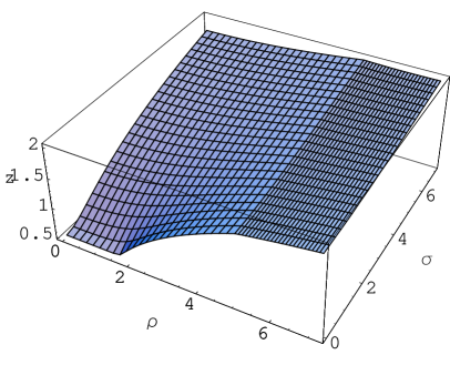
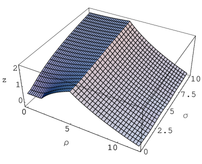
Figure 2: Numerical approximations to the function $z(\rho,\sigma)$ that enters the metric. Both plotted solutions correspond to fixing $c=0$ ($\rho_{0}=\sqrt{e}$) and $\rho_{Q}=5$. It is apparent from the graphics the qualitative change of behavior at such values of $\rho$. On the left $N_{f}=N_{c}$. On the right, $N_{f}=6N_{c}$, a non-asymptotically free field theory that eventually hits a Landau pole. This corresponds to $z$ becoming zero at some value of $\rho$, as shown in the graph.

There is a last subtle point that requires discussion before closing this section. We have introduced a number of fundamentals and found new equations that define a new solution. If this new solution still describes a theory with $N_{c}$ colors, equation (2.5) should still hold. Let us now prove so. Comparing to (2.6), the integrals in $\phi_{1},\phi_{2}$ are trivial, but the angle $\theta$ is not manifest in the geometry any more. This problem is solved by noticing that the components of $F_{(3)}$ relevant to this integration (those not containing $d\tilde{\theta}$ or $d\tilde{\varphi}$ can be written as (see (3.6)) $N_{c}g_{s}\alpha^{\prime}dg\wedge d\phi_{2}\wedge d\phi_{1}$ and that, at infinity, the limits of integration in $\theta$ correspond to $(\sigma=0,\rho=\infty)$ and $(\sigma=\infty,\rho=0)$. Then:

$$\int F_{(3)}=4\pi^{2}g_{s}N_{c}\alpha^{\prime}(g|_{((\sigma=\infty,\rho=0)}-g|_{(\sigma=0,\rho=\infty)})=4\pi^{2}g_{s}N_{c}\alpha^{\prime}$$ (3.12)

where the equalities $g|_{(\sigma=\infty,\rho=0)}=0$ and $g|_{(\sigma=0,\rho=\infty)}=-1$ have been used, and also the fact that $g$ is continuous along the integration path. The first equality is trivial since for $\rho<\rho_{Q}$ the solution coincides with the unflavored one so $g$ can be read from (2.22) setting $\theta=0$. The second one will be proved in section 3.3. Thus, since (3.12) coincides with (2.6), the quantization condition still holds in the flavored case.

3.3 Gauge theory features

Let us now study the gauge theory implications of this computation. The $\rho<\rho_{0}$ region is unchanged with respect to section 2 when the fundamentals are present, so in the following, only the $\rho>\rho_{0}$ region is considered. By repeating the argument of [20] reviewed in section 2.2, it is straightforward to generalize (2.27), (2.28) to:

$$\frac{1}{g_{YM}^{2}} = \frac{N_{c}}{4\pi^{2}}(z|_{\sigma=0})\,,$$ (3.13)

$$\theta_{YM} = 2\Big{(}g|_{\sigma=0}+\frac{N_{f}}{2N_{c}}\Theta(\rho-\rho_{Q})\Big{)}N_{c}\phi_{2}$$ (3.14)

Equation (3.9) implies that $g|_{\sigma=0}$ is a constant. Repeating the argument that the solution at small $\rho$ should be the same as the unflavored one, we find (as in (2.24)) $g|_{\sigma=0}=-1$. Thus:

$$\theta_{YM}=-2N_{c}\Big{(}1-\frac{N_{f}}{2N_{c}}\Theta(\rho-\rho_{Q})\Big{)}\phi_{2}$$ (3.15)

One can compute the monodromy of the $\theta_{YM}$ angle when making a full $U(1)_{R}$ rotation through the space of vevs (at a fixed modulus $\rho\Lambda$):

$$\phi_{2}\rightarrow\phi_{2}+4\pi\quad\Rightarrow\quad\frac{\theta_{YM}}{2\pi}\rightarrow\frac{\theta_{YM}}{2\pi}-2\Big{(}2N_{c}-N_{f}\Theta(\rho-\rho_{Q})\Big{)}$$ (3.16)

which depends on $N_{f}\Theta(\rho-\rho_{Q})$, the number of fundamental hypermultiplet masses encircled by the path. This result is in exact agreement with the field theory expectations (for a review, see [28]).

Let us now turn to $g_{YM}$. Using $g|_{\sigma=0}=-1$, it is immediate to integrate (3.13). Imposing that $z$ matches the unflavored solution for $\rho<\rho_{Q}$ and is continuous at $\rho=\rho_{Q}$, one obtains:

$$\frac{1}{g_{YM}^{2}}=\frac{1}{4\pi^{2}}\Big{[}\Big{(}N_{c}-\frac{N_{f}}{2}\Theta(\rho-\rho_{Q})\Big{)}\log\rho+\frac{N_{f}}{2}\Theta(\rho-\rho_{Q})\log\rho_{Q}\Big{]}$$ (3.17)

Using (2.29), the $\beta$-function at an energy scale $\mu$ is straightforwardly computed: $\beta(g_{YM})(\mu)=-\frac{g_{YM}^{3}}{8\pi^{2}}(N_{c}-\frac{N_{f}(\mu)}{2})$ where $N_{f}(\mu)$ is defined as the number of flavors for which the modulus of their masses is smaller than the scale. The fact that matter fields with bigger mass do not contribute is usually an approximate statement, but, due to the radial symmetry, in this case it is exact as will be shown below. Their effect is just to modify the dynamically generated scale $\Lambda$. For $N_{f}\geq 2N_{c}$, the theory loses asymptotic freedom and for $N_{f}>2N_{c}$, it eventually hits a Landau pole. In the gravity solution, this is translated in the fact that when $N_{f}>2N_{c}$, the function $z$ vanishes at some finite $\rho$ and the metric becomes singular. An analogous behavior in a D3D7 solution was discussed in [11].

The holomorphic coupling can be written by using (3.15) and (3.17) (define $u_{Q}=\rho_{Q}\Lambda$):

$$\tau = i\frac{N_{c}}{\pi}\log\frac{u_{0}}{\Lambda}\,,\qquad{\rm for}\ |u|\leq u_{0}\,,$$

$$\tau = i\frac{N_{c}}{\pi}\log\frac{u}{\Lambda}\,,\qquad{\rm for}\ u_{0}\leq|u|\leq u_{Q}\,,$$

$$\tau = i\frac{N_{f}}{2\pi}\log\frac{u_{Q}}{\Lambda}+\frac{i}{\pi}(N_{c}-\frac{N_{f}}{2})\log\frac{u}{\Lambda}\,,\qquad{\rm for}\ |u|\geq u_{Q}\,,$$ (3.18)

This behavior precisely matches the field theory result. The proof is a simple generalization of the one of [16] for the unflavored case. The coupling is given in terms of the so-called prepotential. As argued in [29], non-perturbative contributions to the prepotential vanish in the large $N$ limit as long as one probes the theory far enough from the vevs $|u-a_{i}|\gg N_{c}^{-1}$ (or, in this case, also from the masses of the hypermultiplets). The perturbative prepotential can be read, for instance, from [30]. Slightly adapting conventions in order to match those of [16]:

$${\cal F}=\frac{i}{8\pi}\sum_{i\neq j}(a_{i}-a_{j})^{2}\log\frac{(a_{i}-a_{j})^{2}}{\Lambda^{2}}-\frac{i}{8\pi}\sum_{\alpha=1}^{N_{f}}\sum_{i=1}^{N_{c}}(a_{i}-m_{\alpha})^{2}\log\frac{(a_{i}-m_{\alpha})^{2}}{\Lambda^{2}}$$ (3.19)

The gauge group is broken to $U(1)^{N_{c}}$ due to the vevs of the scalars. We now probe the theory by considering all but one of the vevs in the ring-like distribution and moving around the other one, $u$, so we have $U(1)^{N_{c}-1}\times U(1)$ where the last $U(1)$ corresponds to the probe brane. In the large $N_{c}$ limit, the coupling is:

$$\tau(u)=\frac{\partial^{2}{\cal F}}{\partial u^{2}}=\frac{i}{2\pi}\sum_{i=1}^{N_{c}}\log\frac{(u-a_{i})^{2}}{\Lambda^{2}}-\frac{i}{4\pi}\sum_{\alpha=1}^{N_{f}}\log\frac{(u-m_{\alpha})^{2}}{\Lambda^{2}}$$ (3.20)

In the large $N_{c},N_{f}$ limit, the sum over discrete distributions can be replaced by integrals, namely:

$$\tau(u)=\frac{i}{2\pi}\int d^{2}a{\cal\rho}_{<\Psi>}(a)\log\frac{(u-a)^{2}}{\Lambda^{2}}-\frac{i}{4\pi}\int d^{2}m{\cal\rho}_{m_{Q}}(m)\log\frac{(u-m)^{2}}{\Lambda^{2}}$$ (3.21)

where ${\cal\rho}_{<\Psi>}(a)$, ${\cal\rho}_{m_{Q}}(m)$ are the density distributions of vevs for the adjoints and masses for the fundamentals respectively. The densities must satisfy the normalization $\int d^{2}a{\cal\rho}_{<\Psi>}(a)=N_{c}$, $\int d^{2}m{\cal\rho}_{m_{Q}}(m)=N_{f}$. Therefore, the ring-like distributions are ${\cal\rho}_{<\Psi>}(a)=\frac{N_{c}}{2\pi u_{0}}\delta(|a|-u_{0})$ and ${\cal\rho}_{m_{Q}}(m)=\frac{N_{f}}{2\pi u_{Q}}\delta(|m|-u_{Q})$. Performing the integrals (3.21) and adjusting an additive constant that can be reabsorbed as a rescaling of $\Lambda$ one finds precisely (3.18). The rescaling of $\Lambda$ is what one usually obtains from holomorphic decoupling.

In the context of fractional branes at orbifolds with massless fundamental hypermultiplets, results similar to those reported in this section were presented in [3, 8].

4 Mesonic excitations

This section is devoted to the analysis of the meson-like excitations, both in the quenched and unquenched backgrounds. In order to address this question, let us add an additional flavor to the theory with a mass defined by its position in $\rho,\phi_{2}$. The flavor group is now $U(1)^{N_{f}+1}$. Obviously, the effect in the geometry of this new brane is suppressed by a power $N^{-1}$ and is negligible. Thus, its excitations can be described by considering it a probe in the background described in the previous sections.

The spectrum can be computed by expanding the action to quadratic order in the fluctuations. The analysis is similar to that in [6], where also an ${\cal N}=2$ theory was analyzed. There are, however, important differences in the low energy field theory: apart from having a large number of hypermultiplets, here there is no massless adjoint hypermultiplet.

Let us consider a probe brane extended along $x_{0},x_{1},x_{2},x_{3},\sigma,\phi_{1}$ and sitting at a point defined by $\tilde{\theta}_{q},\tilde{\varphi}_{q},\rho_{q},{\phi_{2}}_{q}$. Its worldvolume action reads (below, string frame will be used, so the metric (2.9) should be multiplied by $e^{\frac{\Phi}{2}}$):

$$S_{D5}=T_{5}\left(-\int d^{6}\xi e^{-\Phi}\sqrt{-P[g]+2\pi\alpha^{\prime}F}+\int P[C_{(6)}]+\frac{(2\pi\alpha^{\prime})^{2}}{2}\int P[C_{(2)}]\wedge F\wedge F\right)$$ (4.1)

although the last term does not contribute at quadratic order, as can be seen by choosing a gauge in which $C_{(2)}=g_{s}N_{c}\alpha^{\prime}\left(g+\frac{N_{f}}{2N_{c}}\Theta(\rho-\rho_{Q})\right)d\phi_{2}\wedge(d\phi_{1}+\cos\tilde{\theta}d\tilde{\varphi})$. We need the expression for the $C_{(6)}$ in the background which is defined as $dC_{(6)}=F_{(7)}=-*F_{(3)}$. Taking the Hodge dual of (3.6), one finds:

$$F_{(7)}=g_{s}N_{c}\alpha^{\prime}dx_{0}\wedge dx_{1}\wedge dx_{2}\wedge dx_{3}\wedge\Big{[}-\frac{g^{\prime}e^{4\Phi}z}{\rho\sigma}\sin\tilde{\theta}d\tilde{\theta}\wedge d\tilde{\varphi}\wedge d\sigma+$$

$$+\frac{\dot{g}z^{2}e^{4\Phi}}{\rho\sigma}\sin\tilde{\theta}d\tilde{\theta}\wedge d\tilde{\varphi}\wedge d\rho-\big{(}g+\frac{N_{f}}{2N_{c}}\Theta(\rho-\rho_{Q})\big{)}\frac{\sigma}{\rho z^{2}}d\rho\wedge d\sigma\wedge(d\phi_{1}+\cos\tilde{\theta}d\tilde{\varphi})\Big{]}$$ (4.2)

Using (3.7)-(3.10), one can write the following simple expression for the RR-potential:

$$C_{(6)}=g_{s}N_{c}\alpha^{\prime}dx_{0}\wedge dx_{1}\wedge dx_{2}\wedge dx_{3}\wedge\left(ze^{2\Phi}\sin\tilde{\theta}d\tilde{\theta}\wedge d\tilde{\varphi}-\frac{\sigma}{z}d\sigma\wedge(d\phi_{1}+\cos\tilde{\theta}d\tilde{\varphi})\right)$$ (4.3)

4.1 Fluctuation of the scalar fields

In order to describe the small fluctuations, the simplest method is to consider the static gauge and use $x_{\mu},\sigma,\phi_{1}$ as worldvolume coordinates. The embedding can be written as:

$$\tilde{\theta}=\tilde{\theta}_{q}+\delta\tilde{\theta}\,\,,\quad\tilde{\varphi}=\tilde{\varphi}_{q}+\delta\tilde{\varphi}\,\,,\quad\rho=\rho_{q}+\delta\rho\,\,,\quad\phi_{2}={\phi_{2}}_{q}+\delta\phi_{2}\,\,,\quad$$ (4.4)

where all the fluctuations depend on $x_{\mu},\sigma,\phi_{1}$. It is immediate to see that at quadratic order, these scalar fluctuations do not mix with those of the worldvolume gauge field which will be studied in the next section. Expanding the action (4.1) up to quadratic order one finds:

$$S = T_{5}g_{s}N_{c}\alpha^{\prime}\int d^{4}xd\phi_{1}d\sigma\Big{[}\frac{1}{2}\frac{\sigma}{z}e^{-2\Phi}g_{s}N_{c}\alpha^{\prime}({\partial_{x}}\delta\rho)^{2}+\frac{1}{2}\sigma({\partial_{\sigma}}\delta\rho)^{2}+\frac{1}{2\sigma}({\partial_{\phi_{1}}}\delta\rho)^{2}+$$ (4.5)

$$+\frac{1}{2}\rho_{q}^{2}\frac{\sigma}{z}e^{-2\Phi}g_{s}N_{c}\alpha^{\prime}({\partial_{x}}\delta\phi_{2})^{2}+\frac{1}{2}\rho_{q}^{2}\sigma({\partial_{\sigma}}\delta\phi_{2})^{2}+\frac{1}{2\sigma}\rho_{q}^{2}({\partial_{\phi_{1}}}\delta\phi_{2})^{2}+$$

$$+\frac{1}{2}g_{s}N_{c}\alpha^{\prime}\sigma({\partial_{x}}\delta\tilde{\theta})^{2}+\frac{1}{2}\sigma ze^{2\Phi}({\partial_{\sigma}}\delta\tilde{\theta})^{2}+\frac{ze^{2\Phi}}{2\sigma}({\partial_{\phi_{1}}}\delta\tilde{\theta})^{2}+$$

$$+\frac{1}{2}g_{s}N_{c}\alpha^{\prime}\sigma\sin^{2}\tilde{\theta}_{q}({\partial_{x}}\delta\tilde{\varphi})^{2}+\frac{1}{2}\sigma ze^{2\Phi}\sin^{2}\tilde{\theta}_{q}({\partial_{\sigma}}\delta\tilde{\varphi})^{2}+\frac{ze^{2\Phi}}{2\sigma}\sin^{2}\tilde{\theta}_{q}({\partial_{\phi_{1}}}\delta\tilde{\varphi})^{2}+$$

$$+ze^{2\Phi}\sin\tilde{\theta}_{q}\left(({\partial_{\sigma}}\delta\tilde{\theta})({\partial_{\phi_{1}}}\delta\tilde{\varphi})-({\partial_{\phi_{1}}}\delta\tilde{\theta})({\partial_{\sigma}}\delta\tilde{\varphi})\right)\Big{]}$$

where $z,\Phi$ should be understood as functions of $\sigma$ at $\rho=\rho_{q}$. We have defined $({\partial_{x}}\delta\rho)^{2}=\eta^{\mu\nu}(\partial_{\mu}\delta\rho)(\partial_{\nu}\delta\rho)$ where $\mu,\nu$ span the four Minkowski directions. The fluctuations of $\delta\rho,\delta\phi_{2}$ are already decoupled and it is very easy to decouple those for $\delta\tilde{\theta},\delta\tilde{\varphi}$. Let us expand the fields as:

$$\delta\rho=\chi_{1}(\sigma)e^{ik\cdot x}\cos(l\phi_{1})\,\,,$$

$$\delta\phi_{2}=\chi_{2}(\sigma)e^{ik\cdot x}\cos(l\phi_{1})\,\,,$$

$$\delta\tilde{\theta}=\frac{\chi_{+}(\sigma)+\chi_{-}(\sigma)}{2}\sin\tilde{\theta}_{q}e^{ik\cdot x}\sin(l\phi_{1})\,\,,$$

$$\delta\tilde{\varphi}=\frac{\chi_{+}(\sigma)-\chi_{-}(\sigma)}{2}e^{ik\cdot x}\cos(l\phi_{1})\,\,.$$ (4.6)

The equation of motion for $\chi_{1},\chi_{2}$ reads:

$$\frac{\sigma}{ze^{2\Phi}}\bar{M}^{2}\chi_{i}+{\partial_{\sigma}}(\sigma{\partial_{\sigma}}\chi_{i})-\frac{l^{2}}{\sigma}\chi_{i}=0\,\,.$$ (4.7)

where we have defined the four-dimensional mass $M^{2}=-k_{\mu}k^{\mu}$ and $\bar{M}^{2}=g_{s}N_{c}\alpha^{\prime}M^{2}$.

The equations for $\chi_{\pm}$ read:

$$\bar{M}^{2}\chi_{\pm}+\frac{1}{\sigma}{\partial_{\sigma}}(\sigma ze^{2\Phi}{\partial_{\sigma}}\chi_{\pm})-\frac{l^{2}ze^{2\Phi}}{\sigma^{2}}\chi_{\pm}\mp\frac{l}{\sigma}{\partial_{\sigma}}(ze^{2\Phi})\chi_{\pm}=0$$ (4.8)

4.2 Fluctuation of the gauge field

The equation of motion for the gauge field at linear order is:

$$\partial_{a}(e^{-\Phi}\sqrt{-\det(P[g])}F^{ab})=0$$ (4.9)

where $a,b$ run over the six worldvolume coordinates and, again, $\mu,\nu$ over the Minkowski four-space and are contracted with the flat metric $\eta_{\mu\nu}$. Let us now choose a Lorentz gauge $\partial_{\mu}A^{\mu}=0$. The following relation is found:

$${\partial_{\phi_{1}}}A_{\phi_{1}}=-\sigma{\partial_{\sigma}}(\sigma A_{\sigma})$$ (4.10)

Defining a transverse polarization tensor $\epsilon_{\mu}$ and expanding:

$$A_{\mu}=\epsilon_{\mu}\chi_{3}(\sigma)e^{ik\cdot x}\cos(l\phi_{1})\,\,,$$

$$A_{\sigma}=\frac{1}{\sigma}\chi_{4}(\sigma)e^{ik\cdot x}\cos(l\phi_{1})\,\,.$$ (4.11)

one finds from (4.9) that $\chi_{3},\chi_{4}$ also satisfy equation (4.7).

4.3 Analysis of the spectrum

It is interesting to notice certain similarity of the equations (4.7), (4.8) with (3.6) and (3.31) of [6], respectively. Thus, the analysis of the spectrum is also similar to the one in [6].

However, the $l$ we have used here is not the eigenvalue of some $J^{2}$ operator acting on the $SU(2)_{R}$ generators, but it is the charge under a $U(1)_{J}\subset SU(2)_{R}$, i.e., the eigenvalue of a $J_{3}$ operator. The relation between the two would require a better understanding. The bosonic content of the generic ($l\geq 2$) ${\cal N}=2$ massive vector multiplet is given by a massive vector and three real scalars in the $\frac{l}{2}$ of $SU(2)_{R}$ and two real scalars in the $\frac{l-2}{2}$ and $\frac{l+2}{2}$.

Since (4.7) is satisfied by $\chi_{i}$, $i=1,2,3,4$, we have in fact a massive vector and three real scalars with the same mass in the same representation of $SU(2)_{R}$. In order to complete the multiplet, two more real scalars with the same mass are needed. They are the $\chi_{\pm}$ of (4.8). This can be shown by mapping equation (4.7) to (4.8), following a procedure used in [31] for a similar case. In fact:

$$\chi_{+,(l=L)}=\sigma^{-L-1}{\partial_{\sigma}}(\chi_{i,(l=L+1)}\sigma^{L+1})$$

$$\chi_{-,(l=L)}=\sigma^{L-1}{\partial_{\sigma}}(\chi_{i,(l=L-1)}\sigma^{1-L})$$ (4.12)

In order to prove this, substitute in (4.7) $l\rightarrow L\pm 1$ and define $F_{\pm}=\sigma^{1\pm L}\chi_{i}$. Multiply the equation by $ze^{2\Phi}\sigma^{\pm L}$ and derive with respect to $\sigma$. Now, substituting ${\partial_{\sigma}}F_{\pm}=\chi_{\pm}\sigma^{1\pm L}$ and multiplying by $\sigma^{-1\mp L}$, one arrives at (4.8) with $l=L$.

Thus, the bosonic fluctuations yield the bosonic content of a tower of ${\cal N}=2$ massive vector multiplets which can be identified with the mesonic excitations of the theory. The fermionic spectrum can be inferred from supersymmetry or could be directly computed along the lines of [32].

The physical, mesonic, excitations should be those satisfying equations (4.7) or (4.8) and moreover being regular at $\sigma=0$ and normalizable as $\sigma\rightarrow\infty$. Normalizability is a problematic issue in this setup due to ill-behaved UV and will be discussed in section 4.4.

About regularity at the origin, one would need that the $\chi$ functions are finite and even (odd) around $\sigma=0$ when $l$ is even (odd). From (4.7), one sees that near $\sigma=0$, $\chi_{i,l}=c_{1}\sigma^{l}+c_{2}\sigma^{-l}$. Clearly, regularity selects $c_{2}=0$ and $\chi_{i,l}\propto\sigma^{l}$ which in fact satisfies the criterion of parity stated above. For the $\chi_{+}$ modes, substituting in (4.12), we find $\chi_{+,l}\propto\sigma^{l}$ which is also fine with the parity condition. Checking the $\chi_{-}$ modes, involves an extra subtlety since substituting the leading $\chi_{i}$ behavior in (4.12) one just gets zero. But from (4.7), noting that near $\sigma=0$, $\dot{z}\propto\sigma$ we see that both $z$ and $e^{2\Phi}$ behave as $k_{1}+k_{2}\sigma^{2}$ where $k_{1},k_{2}$ are some constants. Thus, the subleading behavior of $\chi_{i}$ is described by $c_{1}\sigma^{l}(1+k_{3}\sigma^{2})$, so substituting in (4.12) one also finds $\chi_{-,l}\propto\sigma^{l}$ which, again, is fine.

4.4 Estimate of the mass spectrum

In D5-brane solutions, like the one we are dealing with or the Maldacena-Núñez background, the dilaton diverges in the UV. The supergravity formalism cannot be trusted in that region, and the UV completion of the field theory is a little string theory. Therefore, it is not a surprise that there are problems in the UV when trying to determine the spectrum. In fact, there is no normalizable mode. However, physically, one would expect to have some modification of the UV that cures this problem, since in the dual theory there are, of course, physical excitations. In this section, a regularization procedure similar to those in [33, 34] is proposed, which basically consists of cutting off the ill-behaved region. It is curious to notice the qualitative difference with [35], where glueballs in Maldacena-Núñez were considered. In that case, even though there was no normalizable mode, the authors found that there existed one leading and one subleading mode in the UV and identified the subleading as the physical one (in a different context, the same criterion was also proposed in [36]). In the present case, there is no leading UV mode because the two modes behave as sine and cosine of some function of $\sigma$.

In order to justify the procedure, it is interesting to notice the similarity in the UV of this setup to the D5D5 brane intersection in flat space. Of course, in such a case, there are also no normalizable modes [31, 37]. But in the UV, by a chain of dualities one can connect the system to an M5M5 intersection which indeed has physical normalizable oscillations [37]. Let us define:

$$y=\log\sigma$$ (4.13)

such that equation (4.7) can be written in the Schrodinger form:

$$\frac{d^{2}\chi_{i}}{dy^{2}}-V(y)\chi_{i}=0\,\,.$$ (4.14)

The potential reads:

$$V(y)=l^{2}-\bar{M}^{2}\frac{e^{2y}}{ze^{2\Phi}}$$ (4.15)

where $y\in(-\infty,\infty)$. The function $ze^{2\Phi}$ is implicitly known in the quenched case (see section 2) and can be determined numerically in the unquenched case, as described in 3.2.

For D5D5 intersecting in flat space [37] the potential reads:

$$V(y)=l^{2}-\bar{M}^{2}\frac{e^{2y}}{e^{2y}+1}$$ (4.16)

Figure 3 shows the qualitative similarity between the two cases. For simplicity, the potential (4.15) is plotted for the quenched case, although the qualitative behavior for the unquenched one is the same. From the figure, we see that starting from $y\approx 4\Rightarrow\sigma\approx 50$, all the potentials coincide, i.e., the IR effects are no longer important. It is natural to choose such a scale as a cutoff. In the plot, the UV problem is apparent since $V(y\rightarrow\infty)<0$ and such a Schrödinger potential cannot have a discrete spectrum.

Figure 3: The figure in the left represents the potential (4.15) with fixed $\mbox{$\frac{N_{f}}{N_{c}}=0$},\ \mbox{$l=2$},\ \mbox{$\bar{M}=3$},\ c=-1$ for different values of $\rho_{q}=1,2,3,4$ (the biggest the $\rho_{q}$ the upper is the line). The thick line corresponds to (4.16). The figure on the right is for fixed $\frac{N_{f}}{N_{c}}=0,\ \mbox{$l=2$},\ \mbox{$\bar{M}=3$},\ \rho_{q}=3$ for $c=-1,0,1$. The different lines are almost coincident and the meson masses should not strongly depend on $c$.

The masses can be estimated by applying the WKB method, which should be reliable for large excitation number. Let us focus on equation (4.7). In the notation of appendix A, we have:

$$f=\sigma \Rightarrow f_{1}=f_{2}=s_{1}=r_{1}=1\,\,,$$

$$h=\frac{\sigma}{ze^{2\Phi}} \Rightarrow s_{2}=1\,\,,\ \ r_{2}=-1\,\,,$$

$$p=-\frac{l^{2}}{\sigma} \Rightarrow p_{1}=p_{2}=-l^{2}\,\,,\ \ s_{3}=r_{3}=-1$$ (4.17)

where it was used that $ze^{2\Phi}\sim\sigma^{2}$ (up to logarithms) for large $\sigma$. In fact, the problem for large $\sigma$ appears in this formalism due to the fact that $r_{1}-r_{2}-2$ is zero, but it should be a positive number in order to apply the WKB. Now, suppose that we can change the UV by that of the M5M5 intersection, which would have $r_{2}=-2$ [37] and leave all the rest unchanged. With this, the WKB approximation to the masses reads (A.5):

$$\bar{M}_{WKB}^{2}\approx\frac{\pi^{2}}{\xi^{2}}n(n-1+3l)\,,\qquad n\geq 1$$ (4.18)

where (A.6):

$$\xi=\int d\sigma\sqrt{\frac{h}{f}}=\int_{0}^{\sigma_{cutoff}}d\sigma(ze^{2\Phi})^{-\frac{1}{2}}$$ (4.19)

Now, the problem for large $\sigma$ appears in the fact that this integral is divergent if $\sigma_{cutoff}\rightarrow\infty$. As said above, a natural scale to cut the integral is around $y\approx 4\Rightarrow\sigma\approx 50$. Although this involves some arbitrariness, everything is fixed in terms of a single parameter $\sigma_{cutoff}$ and thus, it should be possible to estimate how the meson masses depend on the physical parameters $c,\rho_{q},N_{f},\rho_{Q}$.

Figure 4 shows such a dependence in the quenched case, which is easier to deal with since there is an expression for $z$ (2.21) and no numerical integration of a system of PDEs is needed. The quantity $\xi^{-1}$, proportional to the meson mass, is plotted versus $\rho_{q}$. The graph on the left shows how changing $\sigma_{cutoff}$ does not change the qualitative properties of the graph, although of course shifts $\xi$. The graph on the right, shows the behavior for different values of $c$ (related to $\rho_{0}$ by (2.23)). For $\rho_{q}\gg\rho_{0}$, the curves become degenerate as expected on general grounds. The minimal value for the meson masses is attained at $\rho_{q}=\rho_{0}$. It is natural to conjecture that this is due to the fact that when $<\Psi>=m_{q}$ for some of the eigenvalues, there are cancellations between the superpotential term (3.1) and the mass term yielding effectively massless quarks.

Figure 4: On the left, $\xi^{-1}$ versus $\rho_{q}$ for $c=0$. Starting from above, the three lines correspond to $\sigma_{cutoff}=50,70,90$. On the right, $\xi^{-1}$ versus $\rho_{q}$ with fixed $\sigma_{cutoff}=50$ for $c=0,2,4$. In both plots, $\frac{N_{f}}{N_{c}}\rightarrow 0$.

An important question is how the quantum effects produced by unquenched flavor affect the spectrum of physical excitations. From the discussion of section 3.2, it is clear that for $\rho_{q}\leq\rho_{Q}$ the spectrum is unchanged by the unquenched fundamentals. When $\rho_{q}>\rho_{Q}$, the computation requires a delicate numerical analysis of the PDE (3.11) in order to obtain the function $ze^{2\Phi}(\sigma)$ for given ($\frac{N_{f}}{N_{c}},\rho_{Q},\rho_{q},c$). I could not find any significative change of the meson masses when the $N_{f}\sim N_{c}$ hypers are introduced, even when $\rho_{q}>\rho_{Q}$. However, this conclusion should be taken with a grain of salt due to the difficulty of obtaining a precise numerical solution near $\sigma=0$ and also for $\rho_{q}\gg\rho_{Q}$.

Appendix A Appendix: WKB approximation, useful formulae

This appendix collects the results and notation of [38] concerning the WKB approximation. They have been used in section 4.4. Consider a differential equation:

$$\partial_{\sigma}(f(\sigma)\partial_{\sigma}\phi)+(M^{2}h(\sigma)+p(\sigma))\phi=0$$ (A.1)

where the functions $f$,$h$,$p$ behave near $\sigma\rightarrow 0$, $\sigma\rightarrow\infty$ as:

$$f\approx f_{1}\sigma^{s_{1}}\,,\qquad h\approx h_{1}\sigma^{s_{2}}\,,\qquad p\approx p_{1}\sigma^{s_{3}}\,,\qquad(\sigma\rightarrow 0)$$

$$f\approx f_{2}\sigma^{r_{1}}\,,\qquad h\approx h_{2}\sigma^{r_{2}}\,,\qquad p\approx p_{2}\sigma^{r_{3}}\,,\qquad(\sigma\rightarrow\infty).$$ (A.2)

The WKB approximation is consistent provided $s_{2}-s_{1}+2$; $r_{1}-r_{2}-2$ are positive numbers and $s_{3}-s_{1}+2$; $r_{1}-r_{3}-2$ are positive or zero. Define:

$$\alpha_{1}=s_{2}-s_{1}+2\,,\qquad\beta_{1}=r_{1}-r_{2}-2$$ (A.3)

and

$$\alpha_{2}=|s_{1}-1|\qquad{\rm or}\qquad\alpha_{2}=\sqrt{(s_{1}-1)^{2}-4\frac{p_{1}}{f_{1}}}\qquad({\rm if}\ \ s_{3}-s_{1}+2=0)$$

$$\beta_{2}=|r_{1}-1|\qquad{\rm or}\qquad\beta_{2}=\sqrt{(r_{1}-1)^{2}-4\frac{p_{2}}{f_{2}}}\qquad({\rm if}\ \ r_{1}-r_{3}-2=0)$$ (A.4)

The masses are approximated by:

$$M^{2}=\frac{\pi^{2}}{\xi^{2}}n(n-1+\frac{\alpha_{2}}{\alpha_{1}}+\frac{\beta_{2}}{\beta_{1}})+{\cal O}(n^{0})\,,\quad n\geq 1$$ (A.5)

with:

$$\xi=\int_{0}^{\infty}d\sigma\sqrt{\frac{h}{f}}$$ (A.6)

References

• [1] J. M. Maldacena, “The large N limit of superconformal field theories and supergravity,” Adv. Theor. Math. Phys.  2, 231 (1998) [Int. J. Theor. Phys.  38, 1113 (1999)] [arXiv:hep-th/9711200].
• [2] M. Grana and J. Polchinski, “Gauge / gravity duals with holomorphic dilaton,” Phys. Rev. D 65, 126005 (2002) [arXiv:hep-th/0106014].
• [3] M. Bertolini, P. Di Vecchia, M. Frau, A. Lerda and R. Marotta, “N = 2 gauge theories on systems of fractional D3/D7 branes,” Nucl. Phys. B 621, 157 (2002) [arXiv:hep-th/0107057].
• [4] A. Karch and L. Randall, “Open and closed string interpretation of SUSY CFT’s on branes with boundaries,” JHEP 0106, 063 (2001) [arXiv:hep-th/0105132].
• [5] A. Karch and E. Katz, “Adding flavor to AdS/CFT,” JHEP 0206, 043 (2002) [arXiv:hep-th/0205236].
• [6] M. Kruczenski, D. Mateos, R. C. Myers and D. J. Winters, “Meson spectroscopy in AdS/CFT with flavour,” JHEP 0307, 049 (2003) [arXiv:hep-th/0304032].
• [7] N. Seiberg, “Electric - magnetic duality in supersymmetric nonAbelian gauge theories,” Nucl. Phys. B 435, 129 (1995) [arXiv:hep-th/9411149].
• [8] M. Bertolini, P. Di Vecchia, M. Frau, A. Lerda and R. Marotta, “More anomalies from fractional branes,” Phys. Lett. B 540, 104 (2002) [arXiv:hep-th/0202195].
• [9] H. Nastase, “On Dp-Dp+4 systems, QCD dual and phenomenology,” arXiv:hep-th/0305069.
• [10] B. A. Burrington, J. T. Liu, L. A. Pando Zayas and D. Vaman, “Holographic duals of flavored N = 1 super Yang-Mills: Beyond the probe approximation,” JHEP 0502, 022 (2005) [arXiv:hep-th/0406207].
• [11] I. Kirsch and D. Vaman, “The D3/D7 background and flavor dependence of Regge trajectories,” Phys. Rev. D 72, 026007 (2005) [arXiv:hep-th/0505164].
• [12] R. Casero, C. Nunez and A. Paredes, “Towards the string dual of N = 1 SQCD-like theories,” Phys. Rev. D 73, 086005 (2006) [arXiv:hep-th/0602027].
• [13] S. A. Cherkis and A. Hashimoto, “Supergravity solution of intersecting branes and AdS/CFT with flavor,” JHEP 0211, 036 (2002) [arXiv:hep-th/0210105].
• [14] J. Erdmenger and I. Kirsch, “Mesons in gauge / gravity dual with large number of fundamental fields,” JHEP 0412, 025 (2004) [arXiv:hep-th/0408113].
• [15] M. Gomez-Reino, S. Naculich and H. Schnitzer, “Thermodynamics of the localized D2-D6 system,” Nucl. Phys. B 713, 263 (2005) [arXiv:hep-th/0412015].
• [16] J. P. Gauntlett, N. Kim, D. Martelli and D. Waldram, “Wrapped fivebranes and N = 2 super Yang-Mills theory,” Phys. Rev. D 64, 106008 (2001) [arXiv:hep-th/0106117].
• [17] F. Bigazzi, A. L. Cotrone and A. Zaffaroni, “N = 2 gauge theories from wrapped five-branes,” Phys. Lett. B 519, 269 (2001) [arXiv:hep-th/0106160].
• [18] J. M. Maldacena and C. Nunez, “Supergravity description of field theories on curved manifolds and a no go theorem,” Int. J. Mod. Phys. A 16, 822 (2001) [arXiv:hep-th/0007018].
• [19] K. Hori and A. Kapustin, “Worldsheet descriptions of wrapped NS five-branes,” JHEP 0211, 038 (2002) [arXiv:hep-th/0203147].
• [20] P. Di Vecchia, A. Lerda and P. Merlatti, “N = 1 and N = 2 super Yang-Mills theories from wrapped branes,” Nucl. Phys. B 646, 43 (2002) [arXiv:hep-th/0205204].
• [21] F. Bigazzi, A. L. Cotrone, M. Petrini and A. Zaffaroni, “Supergravity duals of supersymmetric four dimensional gauge theories,” Riv. Nuovo Cim.  25N12, 1 (2002) [arXiv:hep-th/0303191].
• [22] U. Gursoy and C. Nunez, “Dipole deformations of N = 1 SYM and supergravity backgrounds with U(1) x U(1) global symmetry,” Nucl. Phys. B 725, 45 (2005) [arXiv:hep-th/0505100].
• [23] F. Bigazzi, R. Casero, A. L. Cotrone, E. Kiritsis and A. Paredes, “Non-critical holography and four-dimensional CFT’s with fundamentals,” JHEP 0510, 012 (2005) [arXiv:hep-th/0505140].
• [24] D. Israel, A. Pakman and J. Troost, Nucl. Phys. B 722, 3 (2005) [arXiv:hep-th/0502073].
• [25] S. Murthy, “Notes on non-critical superstrings in various dimensions,” JHEP 0311, 056 (2003) [arXiv:hep-th/0305197].
• [26] J. Erdmenger, J. Grosse and Z. Guralnik, “Spectral flow on the Higgs branch and AdS/CFT duality,” JHEP 0506, 052 (2005) [arXiv:hep-th/0502224].
• [27] E. Kiritsis, C. Kounnas, P. M. Petropoulos and J. Rizos, “Five-brane configurations without a strong coupling regime,” Nucl. Phys. B 652, 165 (2003) [arXiv:hep-th/0204201].
• [28] M. E. Peskin, “Duality in supersymmetric Yang-Mills theory,” arXiv:hep-th/9702094.
• [29] A. Buchel, A. W. Peet and J. Polchinski, “Gauge dual and noncommutative extension of an N = 2 supergravity solution,” Phys. Rev. D 63, 044009 (2001) [arXiv:hep-th/0008076].
• [30] A. Marshakov, A. Mironov and A. Morozov, “More evidence for the WDVV equations in N = 2 SUSY Yang-Mills theories,” Int. J. Mod. Phys. A 15, 1157 (2000) [arXiv:hep-th/9701123].
• [31] R. C. Myers and R. M. Thomson, “Holographic mesons in various dimensions,” JHEP 0609, 066 (2006) [arXiv:hep-th/0605017].
• [32] I. Kirsch, “Spectroscopy of fermionic operators in AdS/CFT,” JHEP 0609, 052 (2006) [arXiv:hep-th/0607205].
• [33] L. Ametller, J. M. Pons and P. Talavera, “On the consistency of the N = 1 SYM spectra from wrapped five-branes,” Nucl. Phys. B 674, 231 (2003) [arXiv:hep-th/0305075].
• [34] C. Nunez, A. Paredes and A. V. Ramallo, “Flavoring the gravity dual of N = 1 Yang-Mills with probes,” JHEP 0312, 024 (2003) [arXiv:hep-th/0311201].
• [35] E. Caceres and C. Nunez, “Glueballs of super Yang-Mills from wrapped branes,” JHEP 0509, 027 (2005) [arXiv:hep-th/0506051].
• [36] D. Arean, A. Paredes and A. V. Ramallo, “Adding flavor to the gravity dual of non-commutative gauge theories,” JHEP 0508, 017 (2005) [arXiv:hep-th/0505181].
• [37] D. Arean and A. V. Ramallo, “Open string modes at brane intersections,” JHEP 0604, 037 (2006) [arXiv:hep-th/0602174].
• [38] J. G. Russo and K. Sfetsos, “Rotating D3 branes and QCD in three dimensions,” Adv. Theor. Math. Phys.  3, 131 (1999) [arXiv:hep-th/9901056].