Plasma balls/kinks as solitons of large $N$ confining gauge theories

Abstract:

We discuss finite regions of the deconfining phase of a confining gauge theory (plasma balls/kinks) as solitons of the large $N$, long wavelength, effective Lagrangian of the thermal gauge theory expressed in terms of suitable order parameters. We consider a class of confining gauge theories whose effective Lagrangian turns out to be a generic 1 dim. unitary matrix model. The dynamics of this matrix model can be studied by an exact mapping to a non-relativistic many fermion problem on a circle. We present an approximate solution to the equations of motion which corresponds to the motion (in Euclidean time) of the Fermi surface interpolating between the phase where the fermions are uniformly distributed on the circle (confinement phase) and the phase where the fermion distribution has a gap on the circle (deconfinement phase). We later self-consistently verify that the approximation is a good one. We discuss some properties and implications of the solution including the surface tension which turns out to be positive. As a by product of our investigation we point out the problem of obtaining time dependent solutions in the collective field theory formalism due to generic shock formation.

1 Introduction

The study of black holes using the AdS/CFT was initiated by Witten’s observations that black hole spacetimes in $AdS_{5}$ are holographic duals of the deconfinement phase of the four dimensional SU(N) gauge theory on the boundary of $AdS_{5}$ [1]. Various subsequent studies explored this connection to discuss the dynamics and phases of the gauge theory and the physics of black holes [2] -[26].

In a recent paper [15] two of us (PB, SRW) discussed the small Schwarzschild blackhole-string transition in $AdS_{5}\times S^{5}$ by relating it in the gauge theory to the large N [29, 30] transition, and its smoothening by non-perturbative effects. An important feature of studying the Schwarzschild blackhole in $AdS_{5}\times S^{5}$ is that the blackhole is uniformly spread on the $S^{3}$ at the boundary where the gauge theory lives. This is consistent with the fact that the scale invariance of the dual gauge theory is broken only by thermal boundary conditions. Consequently one can discuss the blackhole-string transition in terms of a unitary matrix model, where the unitary matrix (the thermal order parameter) is uniformly spread over $S^{3}$.

In this work we would like to focus on confining gauge theories which have two length scales: the confinement scale $\Lambda$ and the temperature $T=\beta^{-1}$. The relevant order parameters in such theories have a spatial variation on the scale of $\Lambda^{-1}$. The gravity duals of these theories have blackhole solutions which are localized on the boundary. It has been argued in [25, 14], that their holographic dual corresponds, in the large N limit, to a localised region of the deconfinement phase. This object has been called the plasma ball in [14], and it has a mass and a lifetime of $o(N^{2})$. A qualitative gauge theory discussion in [14] uses a balancing of positive surface tension and negative pressure inside the plasma ball, to argue for its existence.

There is no doubt that it is important to study the plasma ball and its dynamics. Besides its utility for the physics of gauge theories at finite temperature, it is one more concrete laboratory for testing and studying various conundrums presented by blackholes [27]. The fact that the blackhole dual is localized on the boundary provides a greater handle on studying the horizon and what lies behind it.

Before we begin to make headway into an understanding of these problems, we need to have a dynamical handle on the plasma ball in the gauge theory. This is a standard hard strong coupling problem. Here by strong coupling we mean large t’ Hooft coupling $\lambda=Ng_{YM}^{2}$. One natural strategy is to use numerical techniques. However a direct numerical approach is also difficult without developing a formalism within which we can ask the right questions.

We present a partial answer to this question in this work. We will discuss the plasma ball as a large N soliton which can be discussed in terms of various order parameters which distinguish between the confinement or deconfinement phases of the gauge theory. In order to do a concrete calculation we will focus on a concrete model that was discussed in [14] in which an interpolating solution was found between two bulk solutions of type IIB string theory: the AdS soliton [4] and a blackbrane. Both solutions are asymptotically $R^{2}\times S_{\tau}^{1}\times S_{\theta}^{1}$, where $S_{\tau}^{1}$ is the thermal circle of radius $\beta$ and $S_{\theta}^{1}$ is a Scherk-Schwarz spatial circle of radius $2\pi$. The corresponding gauge theory is a Scherk-Schwarz compactification of ${\cal N}=4$ $SU(N)$ gauge theory, on $R^{2}\times S_{\tau}^{1}\times S_{\theta}^{1}$. The relevant and natural order parameters of this gauge theory are the holonomies of the gauge field around $S_{\tau}^{1}\times S_{\theta}^{1}$. In fact for technical reasons we will compactify $R^{2}$ to a Scherk-Schwarz cylinder, so that the Euclidean spacetime of the gauge theory is $R^{1}\times S_{\tau}^{1}\times S_{\theta}^{1}\times S_{\alpha}^{1}$. The radius of $S_{\alpha}^{1}$ is chosen larger than that of the $S_{\tau}^{1}$ and $S_{\theta}^{1}$ .

We discuss the effective action of the gauge theory in the long wavelength expansion defined by the confinement scale $\Lambda$. The effective action, in the axial gauge along the non-compact direction $x$, is a one dimensional model of three unitary matrices $U$($x$), $V$($x$) and $W$($x$) corresponding to the zero modes of the Wilson loops on $S_{\tau}^{1}\times S_{\theta}^{1}\times S_{\alpha}^{1}$. Using the fact that we are working with a confining gauge theory of adjoint fields which are all short ranged (of the order of $\Lambda^{-1}$) one can integrate out V($x$) and W($x$) to arrive at an effective action involving the single unitary matrix U($x$), which has the general form

$$S=\Lambda^{-1}\int^{\infty}_{-\infty}dxf(U)\textrm{tr}(\partial_{x}U\partial_{x}U^{\dagger})+g(U)$$ (1)

where $\Lambda^{-1}$ is the confinement scale, and $f(U)$ and $g(U)$ are gauge invariant functions of $U$. $f(U)$ and $g(U)$ contain the information that the gauge theory has a first order confinement/deconfinement phase transition.

It is possible to discuss soliton solutions of the general multi-trace model using the Hamiltonian formulation together with the method of dealing with multi-trace operators developed in [15]. However in order to exhibit a solution we simplify the effective action even further and present the soliton (plasma kink) solution. It turns out to be the motion of the Fermi surface of the many fermion problem that is equivalent to the matrix model in the $SU(N)$ invariant sector. This solution interpolates between the confinement and deconfinement phases and has energy density peaked at the phase boundary.

In our investigations we realized that it is imperative to use the $2+1$ dimensional phase space formulation of the classical Fermi fluid theory. The collective field formalism, which is a hydrodynamical description in $1+1$ dimensions inevitably leads to shock formation and singularities. It is not clear whether a finite energy density soliton solution can be obtained within collective field theory. The shocks are spurious singularities due to the collective field description which correspond to the folds on the Fermi surface, which are inevitable.

The plan of the paper is as follows. In section 2 we describe the two bulk geometries- the AdS soliton [4] and the black brane solution, for which an interpolating domain wall solution was constructed in [14]. In section 3, we present a qualitative discussion as to how one can arrive at an effective description of the thermal gauge theory in terms of the holonomy matrices around the various cycles of the boundary, starting from a four dimensional gauge theory compactified on Scherk-Schwarz circles. For technical reasons we will be working with a gauge theory compactified on two Scherk-Schwarz circles. One can have two dual effective descriptions, in terms of either the Polyakov line or the Wilson loop over the spatial cycle. We present the general class of such effective matrix models. In the following sections we will be working with a particular matrix model belonging to this class. This model can be discussed in terms of an exact fermionic description [28, 30, 31, 32, 33, 34, 35]. We shall also discuss the collective field equations [36] and indicate that their solution develops shocks in finite time.

In section 4 we discuss the phase structure of the model. This model has two stable phases: the confined and deconfined phases, and it undergoes a first order phase transition at a particular temperature. Later in the section we construct the soliton (kink) solution which interpolates between the two phases at the phase transition temperature. We then discuss some of the properties of the solution, in particular the surface tension of the soliton is discussed. We also present the localised (in one dimension) soliton solution at temperatures greater than the phase transition temperature, which approaches the confined phase in the two ends, and discuss some of it’s properties.

In appendix A we show that starting from the confined phase of the theory, where the density of eigenvalues of the Polyakov line is uniform, we reach the clumped eigenvalue distribution only asymptotically, and never in any finite time. In appendix B we discuss the relation of the shocks formed in the collective field theory description to the formation of folds in the Fermi description.

2 Plasma ball in the large $N$ gauge theory and dual black holes

A plasma ball is a localized spherically symmetric bubble of the deconfining phase of a confining gauge theory. In [14] using the AdS/CFT correspondence, their existence was inferred by exhibiting a bulk solution that interpolates between the AdS Soliton[4] and the black-brane solution. The AdS soliton (AdSS), is given by the metric,

$$ds^{2}=L^{2}\alpha^{{}^{\prime}}(e^{+2u}(d\tau^{2}+T_{2\pi}d\theta^{2}+d\omega^{2}_{i})+\frac{1}{T_{2\pi}(u)}du^{2})$$ (2)

where,

$$T_{2\pi}(u)=1-(\frac{1}{2}(d+1)e^{u})^{-(d+1)}$$ (3)

In this paper we will be working with $d=3$. The coordinate $\theta$ is periodic with periodicity $2\pi$, and $\tau$ is the angular coordinate along the thermal circle of the Euclidean theory, with periodicity $\tau\rightarrow\tau+\beta$, and the $\omega_{i}$ are the two non-compact coordinates, while $u$ is the radial coordinate. The boundary topology is $R^{2}\times S^{1}_{\tau}\times S^{1}_{\theta}$, where $S^{1}_{\tau}$ and $S^{1}_{\theta}$ are the thermal and spatial cycles respectively. From the expression for $T_{2\pi}$, one sees that the spatial circle shrinks to zero size at a finite value of $u$.

The black-brane (BB) geometry is given by the metric

$$ds^{2}=L^{2}\alpha^{{}^{\prime}}(e^{+2u}(T_{\beta}d\tau^{2}+d\theta^{2}+d\omega^{2}_{i})+\frac{1}{T_{\beta}(u)}du^{2}$$ (4)

with $T_{\beta}(u)=1-(\frac{\beta}{4\pi}(d+1)e^{u})^{-(d+1)}$. This metric continued to Lorentzian signature has a horizon. Notice that when $\beta=2\pi$, the two metrics 2 and 4 are simply obtained from one other by interchanging the thermal circle with the spatial circle. Since geometrically there is no difference between the two, the free energy of the two configurations must be the same at this temperature. For $\beta<2\pi$, the free energy of the BB geometry dominates the path integral while for $\beta>2\pi$, the free energy of the AdSS geometry is dominant. In [14] a domain wall solution which interpolates between these two solutions was constructed. Clearly such a domain wall solution exists only for $\beta=2\pi$ when the free energy of the two phases is equal. The domain wall is independent of one of the non-compact direction and in the other non-compact direction the BB and AdSS geometry are asymptotically reached at the two ends.

These solutions can be incorporated within the IIB string theory by compactifying on $S^{5}$, with the five-form RR flux turned on. This would then have a dual boundary description in terms of the Scherk-Schwartz compactification of the ${\cal N}=4$ $SU(N)$ SYM theory on a spatial cycle, with thermal boundary condition on both the cycle $S^{1}_{\tau}$ and $S^{1}_{\theta}$. The gauge theory lives on $R^{2}\times S^{1}_{\tau}\times S^{1}_{\theta}$. At $\beta=2\pi$ clearly the two circles are identical and can be interchanged.

The above discussion suggests that a ball of large but finite radius of the deconfined plasma can occur as a solution to the finite temperature effective action of the gauge theory, at a temperature slightly above $T_{c}$. At $T=T_{c}$ there exists a kink solution interpolating between the confined and deconfined phases.

3 Gauge theories on $R^{2}\times S^{1}_{\tau}\times S^{1}_{\theta}$

From the AdS/CFT correspondence, these bulk geometries- the AdSS geometry and the BB geometry correspond in the thermal gauge theory to the confinement and deconfinement phases respectively [1]. These phases are characterised by the expectation value of the Polyakov line, which is the trace of the holonomy around the thermal circle,

$$U(w_{1},w_{2},\theta)={\cal P}\exp(-\oint A_{\tau}d\tau)$$ (5)

$w_{i}$ are the two non-compact coordinates and the $\theta$ is the angular coordinate along the spatial circle, while ${\cal P}$ denotes path ordering. In particular, the expectation value of $\textrm{tr}\ U$ vanishes in the confined phase while in the deconfined phase it takes a non-zero value . Similarly one can define the holonomy around the spatial cycle $S^{1}_{\theta}$.

$$V(w_{1},w_{2},\tau)={\cal P}\exp(-\oint A_{\theta}d\theta)$$ (6)

Since the role of the two circles are interchanged in the two bulk geometries, it follows from the AdS/CFT correspondence, that $\textrm{tr}V=0$ in the deconfined phase, and it is non-zero in the confined phase . At $\beta=2\pi$, because the two geometries are identical under the interchange of the thermal and spatial circles, the effective action in terms of $V$ should be identical to the one in terms of $U$. Later in this section we will qualitatively argue as to how one can arrive at an effective action in terms of both $U$ and $V$ and then in terms of either $U$ or $V$, starting from the four-dimensional gauge theory.

Since we will mainly be interested in the solution which interpolates between the confinement and deconfinement phases as a function of one of the non-compact direction, it should be possible to find the one dimensional kink solution in an effective one-dimensional unitary matrix model. In order to realize this in a gauge theory at large $N$, it turns out to be convenient to work with $R\times S_{\tau}^{1}\times S_{\theta}^{1}\times S^{1}_{\alpha}$, where the $S^{1}_{\alpha}$ is the spatial circle, obtained by compactifying a noncompact direction previously labelled by the coordinate $w_{2}$. We introduce the holonomy along the spatial cycle $S^{1}_{\alpha}$

$$W(w_{1},\tau,\theta)={\cal P}\exp(-\oint A_{\alpha}d\alpha)$$ (7)

This would correspond to replacing one of the non-compact directions of the bulk geometry that we discussed earlier, with a circle without changing the solution. Henceforth we shall set the noncompact direction $w_{1}\equiv x$.

3.1 Effective action in terms of the Polyakov lines and Wilson loops

The bosonic part of the action of the general gauge theory will be written in terms of the gauge degrees of freedom $A_{1}$, $A_{\tau}$, $A_{\theta}$, $A_{\alpha}$ as well as the scalar fields $\Phi_{i}$ which transform in the adjoint representation. Here $A_{1}$ corresponds to the gauge field in the non-compact direction and we can choose the axial gauge $A_{1}=0$. These fields are in general functions of $(x,\theta,\tau,\alpha)$. Since the Scherk-Schwarz compactification breaks supersymmetry, the fermions are massive and the scalar fields get mass at one loop from quantum corrections. They can therefore be integrated out from the quantum effective action. Fourier expanding the gauge fields in all the circles and integrating out all the higher KK modes around every circle, we get a effective theory in terms of the zero modes of the fields: $A^{0}_{\tau}(x)$, $A^{0}_{\theta}(x)$, $A^{0}_{\alpha}(x)$.

This effective theory in terms of the zero modes is gauge invariant, and therefore we should be able to write it down in terms of the zero modes of the the holonomy matrices $U$,$V$ and $W$. From now on we will use the notation $U$, $V$, $W$, to denote the zero modes of the above holonomy matrices.

The effective action will be a function of all possible gauge invariant operators. The gauge invariant operators are constructed out of the $Z_{N}$ invariant products of the polynomials of $U$, $V$ and $W$ and their covariant derivatives, $D_{x}U$, $D_{x}V$, $D_{x}W$, and are of the form $\Pi_{i}\textrm{tr}(U^{l_{i}}V^{m_{i}}W^{p_{i}}(D_{x}U)^{n_{i}}...)$, where the exponents $l_{i}$, $m_{i}$, $p_{i}$, $n_{i}$,etc are integers, such that the sum of all the exponents $\sum_{i}l_{i}+m_{i}+p_{i}+n_{i}+...=0$. In the gauge $A_{1}=0$, the covariant derivatives are the same as the ordinary derivatives. At sufficiently long wavelengths we neglect the higher derivative terms which are suppressed by powers of the confining scale $\Lambda^{-1}$.

Depending on which of the holonomy matrices condense, there will be three phases in the gauge theory. In the BB phase $\textrm{tr}U\neq 0$, $\textrm{tr}V=0$ and $\textrm{tr}W=0$. In the other two phases one of the spatial holonomy matrices $V$ or $W$ will get expectation values, while the expectation value for the other two vanish. However we are interested in an interpolating solution between the black brane and the AdS soliton, and not in the transitions involving all the three cycles. If we choose the radius $R_{(}S^{1}_{\alpha})>R(S^{1}_{\tau}),\ R(S^{1}_{\theta})$, at the temperature of interest, then from the supergravity solution it follows that the cycle $S^{1}_{\alpha}$ never shrinks and corresponds to $\langle W\rangle=0$ in the gauge theory. We can therefore put $W=0$ in the effective three matrix model to once again obtain a two matrix model. The action for this will in general be very complicated, with all terms that are allowed by gauge invariance. It will contain words of the type $\textrm{tr}(U^{n_{1}}V^{n_{2}}U^{n_{3}}....)$, and also derivative terms. The general action in the long wavelength expansion will be of the form,

$$S_{eff} = \Lambda^{-1}\int dxf_{1}(U,V)\textrm{tr}|\partial_{x}U|^{2}+f_{2}(U,V)\textrm{tr}|\partial_{x}V|^{2}+$$

$$f_{3}(U,V)\textrm{tr}(\partial_{x}U\partial_{x}V^{\dagger})+f_{4}(U,V)+\textrm{h.c}$$

where, $\Lambda^{-1}$ is the confinement length scale, $f_{i}$’s are gauge invariant functions of arbitrary polynomials of $U$, $V$ and $\beta$ with appropriate factors of $N$. At $\beta=1/2\pi$, when the size of the two cycles are equal, the effective action will be invariant under $U\Rightarrow V$. Integrating over either the $U$ or the $V$ we will get a single matrix model in terms of $V$ or the $U$ matrix.

Since the theory is confining and has a mass gap, we can integrate out the $V$ matrix, without worrying about infrared divergences, and we will be left with a model, given by

$$S=\Lambda^{-1}\int dxf(U)\textrm{tr}(\partial_{x}U\partial_{x}U^{\dagger})+g(U)$$ (9)

where again $\Lambda^{-1}$ is the confinement scale, and $f(U)$ and $g(U)$ are temperature dependent, gauge invariant functions. As in (3.1) we have neglected all the higher derivative terms in the action, which are suppressed by powers of the confining scale. Equivalently we could integrate out $U$ to arrive at a matrix model of $V$.

In the sequel we will mainly study the soliton solution of the simplest of this class of models, given by .

$$S=\Lambda^{-1}\int dxN\textrm{tr}(|\partial_{x}U|^{2})+\xi|\textrm{tr}U|^{2}$$ (10)

Here we will assume that $\xi>0$ which ensures the existence of a first order phase transition at some value of $\xi$. By rescaling $x\rightarrow\Lambda^{-1}x$, we can remove the explicit $\Lambda$ dependence from the above action to get,

$$S=\int dxN\textrm{tr}(|\partial_{x}U|^{2})+\xi|\textrm{tr}U|^{2}$$ (11)

where $x$ is now given in units of $\Lambda^{-1}$. Hence forth we will be using this form of the action.

4 Analysis of the one dimensional matrix model

In this section we will analyze the phase diagram of the unitary matrix model given by the action of the form (10). The matrix model described by the action(10) can be discussed using two methods. One is to use the collective field theory techniques as was done by Jevicki and Sakita[36]. This is basically a collective field description in $1+1$ dimension. The Hamiltonian is written in terms of the density $\rho(\theta,x)$ and velocity $v(\theta,x)=\partial_{\theta}\Pi(\theta,x)$, where $\Pi$ is the canonical conjugate of $\rho$. The $\rho(\theta,x)$ field is the eigenvalue density field constructed out of the matrix $U$,

$$\rho(\theta,x)=\sum^{+\infty}_{n=-\infty}\rho_{n}(x)e^{2i\pi n\theta}$$ (12)

where $\rho_{n}=\frac{1}{N}\textrm{tr}(U^{n})$. For example, from the matrix model described by equation (10), we get the following collective field Hamiltonian,

$$H_{cf}=\int d\theta\ (\frac{\rho v^{2}}{2}+\frac{\pi^{2}\rho^{3}}{6})-\xi|\rho_{1}|^{2}$$ (13)

This Hamiltonian, gives rise to the following set of fluid dynamical equations,

$$\frac{\partial\rho(x,\theta)}{\partial x}+\frac{\partial}{\partial\theta}(\rho(x,\theta)v(x,\theta)) = 0$$ (14)

$$\frac{\partial v(x,\theta)}{\partial x}+v(x,\theta)\frac{\partial v(x,\theta)}{\partial\theta}+\pi^{2}\rho(x,\theta)\frac{\partial\rho(x,\theta)}{\partial\theta} = -2\xi\rho_{1}(x)\sin\theta$$

Here $\theta$ is a periodic variable defined in the range $[-\pi,\pi]$ and $x$ is a variable defined in the range $(-\infty,+\infty)$. The collective field approach is only valid for solutions which are spatially uniform,(for which $v(x,\theta)=0$ and $\frac{\partial}{\partial x}\rho(x,\theta)=0$). The spatially non-uniform solutions generically develop shocks in finite time, after which the collective field equations are not valid.

A correct (and exact) way to analyze the model (10) is to rewrite the model as a theory of interacting fermions [33] with the Hamiltonian (where the ’$x$’ direction is identified with the Euclidean time).

$$H=\int d\theta\psi^{{\dagger}}(\theta)\partial^{2}_{\theta}\psi(\theta)-\xi|\int d\theta e^{i\theta}\psi(\theta)\psi^{{\dagger}}(\theta)|^{2}$$ (15)

In the large $N$ limit the fermion system will be classical and one can use the phase space density, ${\cal U}(p,\theta,x)$ such that,

$$\int\frac{dp}{2\pi}d\theta\ {\cal U}(p,\theta,x)=1$$ (16)

If a phase space cell is occupied then ${\cal U}(p,\theta,x)=1$ or else ${\cal U}(p,\theta,x)=0$. Hence ${\cal U}(p,\theta,x)$ satisfies the relation

$${\cal U}(p,\theta,x)^{2}={\cal U}(p,\theta,x)$$ (17)

The Hamiltonian written in terms of the phase space density is,

$$\frac{H}{N^{2}}=\int dpd\theta\frac{p^{2}}{2}{\cal U}(p,\theta,x)-\xi|\int dpd\theta e^{i\theta}{\cal U}(p,\theta,x)|^{2}$$ (18)

In terms of ${\cal U}(p,\theta,x)$, the density and velocity $\rho(\theta,x)$ and $v(\theta,x)$ are,

$$\rho(\theta,x)=\int\frac{dp}{2\pi}{\cal U}(p,\theta,x),\ v(\theta,x)=\frac{1}{\rho}\int\frac{dp}{2\pi}p\ {\cal U}(p,\theta,x)$$ (19)

In the appendix we will further discuss the relation between the phase space and collective field theory approach and we will interpret the shock formation as the formation of folds on the Fermi surface. Hence the shock singularities are artifacts of the collective field approach and are resolved by a more accurate treatment.

In the following sections we will analyze the solutions of the fermionic Hamiltonian (18). We will start by describing the spatially uniform solution (phases of the theory) and then describe the non-uniform interpolating solution (plasma kink).

4.1 Spatially uniform solutions

Here we analyze those solutions where the density of the eigenvalues of the matrix $U$ is uniform over the direction $x$. In this case the location of the Fermi level will also be constant in $x$. Classically $\rho$ can always be chosen to be an even function of $\theta$. Then the potential in the equation (18) becomes, $\xi(\int dp\frac{d\theta}{2\pi}\cos\theta{\cal U}(p,\theta,x))^{2}$. In the Hatree Fock approximation, the phase space evolution equation for a single particle is,

$$\dot{\theta} = p$$ (20)

$$\dot{p} = -2\xi\rho_{1}(x)\sin\theta$$

Where $\rho_{1}(x)=\int dp\frac{d\theta}{2\pi}\cos\theta{\cal U}(p,\theta,x)$ and $\dot{\theta}\equiv\frac{d}{dx}\theta$, $\dot{p}\equiv\frac{d}{dx}p$. For a spatially uniform solution, $\rho_{1}$ is independent of $x$ and we can integrate the above equations to get,

$$p^{2}=2(E+2\xi\rho_{1}\cos\theta)$$ (21)

where $E$ is the energy of the particle. Therefore for a particle on the Fermi level, we have,

$$\hat{p}_{\pm}=\pm\sqrt{2(E_{f}+2\xi\rho_{1}\cos\theta)}$$ (22)

where $\hat{p}_{\pm}$ correspond to the upper and lower branches of the Fermi level. Consequently

$$\rho(\theta)=\frac{\sqrt{2}}{\pi}\sqrt{E_{f}+2\xi\rho_{1}\cos\theta}.$$ (23)

One has to satisfy the normalization condition given in equation (16) and the self consistency condition for $\rho_{1}$, which effectively solves $E_{f}$ in terms of $\xi$ and $\rho_{1}$

$$\int d\theta\frac{\sqrt{2}}{\pi}\sqrt{E_{f}+2\xi\rho_{1}\cos\theta}=1$$ (24)

$$\int d\theta\frac{\sqrt{2}}{\pi}\cos\theta\sqrt{E_{f}+2\xi\rho_{1}\cos\theta}=\rho_{1}$$

Depending on whether $|\frac{E_{f}}{2\xi\rho_{1}}|<1$ or $|\frac{E_{f}}{2\xi\rho_{1}}|\geq 1$, the integrals in equation(24) will be evaluated between the limits $[-\theta_{0},\theta_{0}]$, with $\theta_{0}<\pi$, or over the full range $[-\pi,+\pi]$. The former case corresponds to the gapped phase, as $\rho(\theta)=0$ outside$[-\theta_{0},\theta_{0}]$.), while the latter case corresponds to the ungapped phase) [30].

One can study the different static phases of the model, by solving the self-consistency and the normalization conditions given in equation (24) simultaneously. This is hard to do analytically, but can be studied numerically. However it would be useful to have an understanding of the various phases as extrema of the potential in terms of $\rho$. This potential can be obtained from the Hamiltonian given in equation (18), using equations (19, 22) to integrate over $p$. We then obtain,

$${\cal H}=\int d\theta\frac{1}{2}\rho v^{2}+V([\rho])$$ (25)

where,

$$V([\rho])=\int d\theta\frac{\pi^{2}\rho^{3}}{6}-\xi|\rho_{1}|^{2}$$ (26)

The potential of the model is actually a function of the infinitely many Fourier modes of $\rho$. Note that the static phases are all of the form given by the equation (23). It is therefore useful to parametrize $\rho$ by

$$\rho=\sqrt{\sum^{\infty}_{n=0}a_{n}\cos(n\theta)}$$ (27)

With this parametrization, the uniform phase solution is given by $a_{0}=\frac{1}{2\pi}$, and all other $a_{n}=0$, while the gapped phase corresponds to $a_{n}=0$, for $n>1$ and $a_{0}$, $a_{1}$ taking appropriate values. With this parametrization, the potential will be a function of the $a_{n}$. Since all the phases of the theory lie in the plane given by $a_{n>1}=0$, it will be enough to restrict to this plane. We therefore parametrize $\hat{p}_{\pm}$ by the following form.

$$\hat{p}_{\pm}=\pm\sqrt{2(E+2\xi C_{1}\cos\theta)}$$ (28)

We determine $E$ in terms of $C_{1}$ by the normalization condition (16). Then substituting this in the expression for the potential, the potential becomes a function of only one parameter $C_{1}$. Then we can numerically calculate the potential given by the equation(26) as a function of $C_{1}$ (see figure 1).

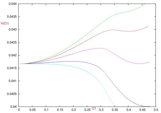
Figure 1: Plot of $V(C_{1})$ with $C_{1}$ with $\xi=0.22$, $\xi=0.23$, $\xi=0.237$, $\xi=0.245$ and $\xi=0.25$, with value of $\xi$ increasing from the top curve to the bottom.

We now summarise the key points from our analysis of the phase structure of the model in consideration.

• At low enough values of $\xi$, there is a single phase where $\rho(\theta)=\frac{1}{2\pi}$ or $\hat{p}_{\pm}=\pm\frac{1}{2}$. Here $C_{1}=0$. This is the uniform phase of the eigenvalue distribution.

• At $\xi=\xi_{n}=0.227$ there is nucleation of two phases for which $\rho(\theta)$ is no more a constant. Both the phases have a gapped eigenvalue distribution. One phase is unstable ($II$) and the other is stable ($III$).

• The first order phase transition between the phase $I$ and phase $III$ occurs at $\xi=\xi_{1}=0.237$ and $C_{1}=0.4408$, $E=0.1711$.

• The phase $I$ becomes locally unstable at $\xi=\xi_{2}=.25$

• At $\xi=\xi_{3}=0.23125$, and $C_{1}=0.3336$, phase $II$ has a gapped to ungapped transition, this is the point of the third order $GWW$ phase transition. [29, 30]

4.2 Spatially non-uniform solutions: plasma kinks

In the previous section we have analyzed the phase structure of our model. In particular we saw that at $\xi=0.237$, the two stable phases (the confining and the deconfining phases) of the model have the same free energy. In this section we will first describe an interpolating domain wall type solution from the deconfined phase to the confining phase, at this value of $\xi$. Later in the section we will also construct a localised soliton solution which reaches the confined phase for large values of $|x|$.

The confining phase is described by a constant Fermi level which is given by the following equations in phase space,

$$\hat{p}_{\pm}=\pm\frac{1}{2}$$ (29)

While in the deconfining phase, the Fermi levels were given by,

$$\hat{p}_{\pm}=\pm\sqrt{2(E+2\xi C_{1}\cos\theta)}$$ (30)

Therefore we are looking for solutions in which the Fermi level evolves from (29) to (30). In terms of the geometry of the Fermi level it is a evolution from a band like to an ellipsoidal structure fig. 2.

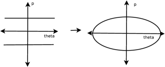
Figure 2: A schematic picture of the Fermi levels.

In terms of $\rho$, the solution has the property,

$$\rho(\theta,x)\rightarrow\frac{1}{2\pi},\quad x\rightarrow-\infty$$ (31)

$$\rho(\theta,x)\rightarrow\frac{\sqrt{2}}{\pi}\sqrt{E+2\xi\rho_{1}\cos\theta},\quad x\rightarrow\infty$$

Now in general the Fermi level will be described by the vanishing of some implicit function $f(\theta,p,x)=0$. In the static case,

$$f(p,\theta)\equiv(p_{+}-\sqrt{E+2\xi C_{1}\cos\theta})(p_{-}+\sqrt{E+2\xi C_{1}\cos\theta})=0$$ (32)

In the general case $f(p,\theta,x)$ is not of this simple form and may have more roots. This corresponds to the case where the upper and lower Fermi levels develop folds and become multi-valued in $\theta$.

As each point in the phase space satisfies the equation, $\dot{\theta}=p,\dot{p}=V^{\prime}(\theta)$, one can derive the time evolution of the function $f$ to be,

$$\partial_{x}f+p\partial_{\theta}f+V^{\prime}(\theta)\partial_{p}f=0$$ (33)

It would be interesting to try and solve the above equations numerically as a boundary value problem. We have not been able to do this. Instead we take a variational approach to the problem, and make a simple but reasonably accurate ansatz for the Fermi level. We will now summarise the main steps of the analysis.

• We choose an ansatz for the Fermi level similar to the form in the static case,

  $$f(p,\theta,x)\equiv(p_{+}-\rho(\theta,x)+v(\theta,x))(p_{-}+\rho(\theta,x)+v(\theta,x))=0$$ (34)

  with $\rho$ given by,

  $$\rho=\frac{\sqrt{2}}{\pi}\sqrt{E(x)+2\xi C_{1}(x)\cos\theta}$$ (35)

  where the $E(x)$, $C_{1}(x)$ are functions of $x$. This would be a good approximation if the $E(x)$, $C_{1}(x)$ are slowly varying functions of $x$. What we are doing in effect is to approximate the actual solution by a two Fermi surface solution throughout the evolution of the system, always given by the two curves $p=\hat{p}_{\pm}$. Therefore $\hat{p}_{\pm}$ are of the form,

  $$\hat{p}_{\pm}=\pm\sqrt{2}\sqrt{E(x)+2\xi C_{1}(x)\cos\theta}+v(\theta,x)$$ (36)

  $E(x)$ is determined in terms of $C_{1}(x)$ by the condition (16) or equivalently

  $$\int d\theta\frac{\sqrt{2}}{\pi}\sqrt{E(x)+2\xi C_{1}(x)\cos\theta}=1$$

  We determine $v(\theta,x)$ by the continuity equation,

  $$\frac{d}{dx}\int{\cal U}(p,\theta,x)dp\frac{d\theta}{2\pi}=0$$ (37)

  The solution of the continuity equation is given by,

  $$v(\theta,x)=\frac{1}{\rho(\theta,x)}(\frac{\partial}{\partial x}\int_{0}^{\theta}d\theta\rho(\tilde{\theta},x)d\tilde{\theta})$$ (38)

• Next, substituting this form of $\rho(\theta,x)$ and $v(\theta,x)$ back into the Hamiltonian and performing the $\theta$ integral, we get,

  $${\cal H}={C^{\prime}_{1}}^{2}K(C_{1})-V(C_{1})$$ (39)

  where $C^{\prime}_{1}=\frac{d}{dx}C_{1}(x)$. Hence the whole problem is reduced to a quantum mechanical problem of $C_{1}(x)$. The function $K(C_{1})$ and $V(C_{1})$ are determined numerically, and $K(C_{1})$ is positive and non-zero. Along the propagation in $x$ the quantity ${\cal H}$ is conserved. This conservation law is used to determine the relation,

  $$\frac{d}{dx}C_{1}=\sqrt{\frac{E+V(C_{1})}{K(C_{1})}}$$ (40)

• The above equation is integrated numerically to obtain $C_{1}(x)$ as a function of $x$. Knowing $C_{1}(x)$ enables us to determine the phase space density ${\cal U}(p,\theta,x)$. The plot of $C_{1}(x)$ as a function of $x$ is shown in figure (3). It should be noted that the soliton rises slowly but approaches the other end relatively fast. This follows from the asymmetric nature of the potential.

  

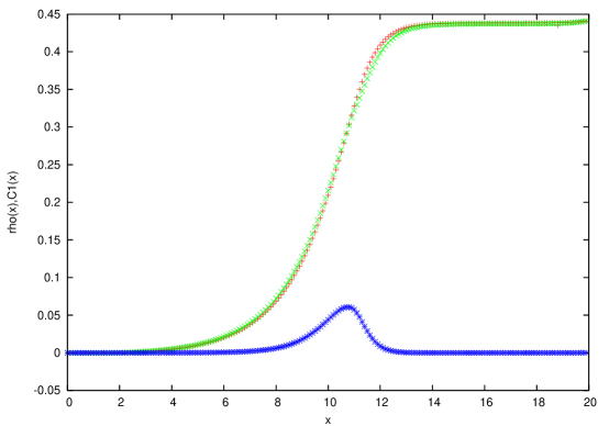
  Figure 3: Plot of $C_{1}(x)$ (green), $\rho(x)$ (red) and free energy density (blue, not in scale)

• It is important to check for the self consistency of this ansatz. This can be done by substituting the $\rho_{1}(x)$ obtained from our ansatz into the single particle equations and see how they evolve in $x$ under this $\rho_{1}$. One can then compute the $\rho_{1}(x)$ obtained from this exact evolution at each instance of $x$, which we denote by $\rho^{a}_{1}(x)$ and compare with $\rho_{1}(x)$ obtained from the ansatz. If $\rho_{1}(x)$ were an exact solution, then one would get $\rho^{a}_{1}(x)=\rho_{1}(x)$. This is checked numerically. We started with $50\times 50$ particles uniformly distributed over the phase space region $p\in[-\frac{1}{2},\frac{1}{2}],\theta\in[0,2\pi]$. This gives us the band like Fermi level in figure 2. We study the evolution of the individual particles under the driving force $2\xi\rho_{1}(x)$ and calculate the $\rho^{a}_{1}(x)$ from the phase space distribution of the particles. We present the plots comparing the two values of $\rho_{1}(x)$, in figure 4.

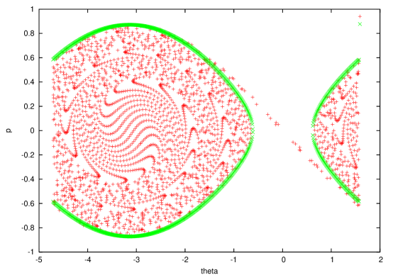
Figure 9: Phase space particles (red) at $x\approx 11.9$ showing the match with Fermi surface (green) in phase III.

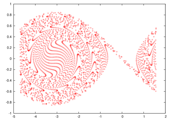
Figure 10: Phase space particles at $x\approx 11.6$ showing shocks at around $\theta\approx-0.8$ and $\theta\approx 0.8$.

• One may also look at the snapshots of the phase space particles. In figures 9 and 10 we have presented two snapshots taken at $x\approx 11.9$ and at $x\approx 11.6$. We see from the plots that the system is driven to the gapped phase configuration to a good accuracy. The phase space snapshot at the later value of $x$ matches very well with the expected Fermi distribution in phase $III$ at $\xi=0.237$. This means that we are indeed reaching very near to the phase $III$.

  We also find that during the evolution of the Fermi sea, folds are formed on the Fermi level. As we discuss in the appendix B this is inevitable. However the area under the folds is a small fraction of the area of the full Fermi surface. This shows that our ansatz of a Fermi level with no folds, is self-consistent.

  One also sees from the phase space plots that, as discussed in appendix A, $\rho(0,x)\neq 0$ for all $x$.

  

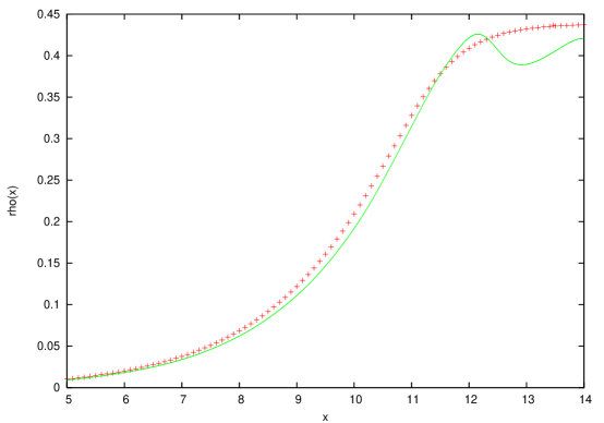
  Figure 4: Plot of $\rho^{a}_{1}(x)$ (green) and $\rho_{1}(x)$ (red) with $x$

• If we continue to plot the evolution of the phase space particles for long times, we will see that the value of $\rho^{a}_{1}(x)$ will start falling from it’s value in the gapped phase, and the particles will disperse away from the ellipsoid as the system will move away from the gapped phase. This happens because even though the $\rho_{1}$ we obtain from our ansatz drives the system very near to the gapped phase starting from the uniform phase (as is evident from the phase space plots), it does not take it exactly to the gapped phase, since no matter how good the ansatz is it is not the exact solution. If we continue to the evolve the system this error will start accumulating and the system will again disperse away from the gapped phase. This problem would not occur if we could do the exact numerical simulation for the soliton in the phase space as a boundary value problem with value of $\rho^{a}_{1}(x)$ fixed at both ends.

An important quantity that we can determine from our solution is the surface tension. The surface tension in general could either be positive or negative at the phase boundary. However, for lagrangians with positive kinetic terms, which is true in our case, the surface tension also turns out to be positive.

In one dimension surface tension is defined as the total free energy of the soliton, which in turn is the total action for the soliton. Hence the surface tension $\sigma$ is, (see [39])

$$\sigma=2\int_{-\infty}^{+\infty}dx\left(V(C_{1}(x))-V_{vacuum}\right)$$ (41)

This quantity at $\xi=\xi_{1}=0.237$ is numerically calculated to be, $\sigma=0.0027$.

4.3 Localized soliton- plasma ball

In the previous section we constructed an interpolating kink solution for $\xi=\xi_{1}$. For $\xi$ between $\xi_{1}$ and $\xi_{2}$, the two minima corresponding to phase $I$ and phase $III$ have different free energies (figure 1) and in particular, the minima corresponding to phase $I$($C_{1}=0$) is a false vacuum. In this case there exists a soliton solution which is localized in the $x$ direction, and which goes to $C_{1}=0$ at both $x\rightarrow\pm\infty$ [40].

Such a solution has a simple interpretation in terms of a particle in real time moving in a potential $-V(x)$. From the conservation of the Hamiltonian (39), it is obvious that if we start from $C_{1}=0$ at $x=0$, the solution never reaches phase $III$. It will bounces from a finite value of $C_{b}$ and comes back to the phase $I$ again, where $C_{b}$ is determined by the relation $V(C_{b})=V(0)$. In Fig 5 we present a schematic plot of $-V(C_{1})$ and the bounce solution.

Figure 5: Plot of $V(C_{1})$ showing the bounce solution below.

As before, one can construct such a solution numerically (see figure 6). This solution has a natural interpretation as a bubble of deconfined plasma within the confined phase. The plots shows two interesting trends. The first one is that the width and height of the soliton both increases as $\xi\rightarrow\xi_{1}=0.237$ from above. The second one is that as $\xi\rightarrow\xi_{2}$, the height of the soliton decreases, but the width of the soliton also increases. Hence width of the soliton comes to a minimum at some value of $\xi$ between $\xi_{1}$ and $\xi_{2}$.

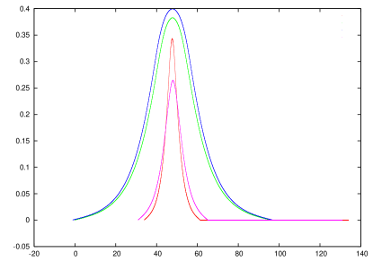
Figure 6: Plot of $C_{1}(x)$ as a function of $x$ at $\xi=0.245$ (violet), $\xi=0.24$ (red), $\xi=0.238$ (green) and $\xi=0.2375$ (blue).

One can define the width $w$ of the localized soliton as a measure of the spread in $x$ over which the value of $C_{1}$ drops to a specified fraction $C_{*}$ of it’s maximum $C_{b}$. As $\xi\rightarrow\xi_{1}$ the localized soliton becomes the semi-infinite soliton discussed in the previous section and consequently the width of the soliton goes to infinity. It would be interesting to calculate the change in the width of the soliton with $\xi$ as $\xi\rightarrow\xi_{1}$. In this limit, $C_{b}$ almost reaches $C_{III}$. The equation of motion is given by,

$$2K(C_{1})C^{{}^{\prime\prime}}_{1}+2K^{\prime}(C_{1})C^{{}^{\prime}2}_{1}=V^{\prime}(C_{1})$$ (42)

where $C^{\prime}_{1}=\frac{d}{dx}C_{1}$, $K^{\prime}(C_{1})=\frac{d}{dC_{1}}K(C_{1})$, and similarly $V^{\prime}(C_{1})=\frac{d}{dC_{1}}V(C_{1})$. Expanding $K(C_{1}),V(C_{1})$ around $C_{1}=C_{III}$, and using the fact that $V^{\prime}(C_{III})=0$, and $C^{\prime}_{1}$ will be small and negligible near $C_{1}=C_{III}$ (because $C_{III}$ is a turning point), we get from equation(42)

$$\frac{d^{2}}{dx^{2}}\delta C_{1}=A(C_{III})\delta C_{1}$$ (43)

where $\delta C_{1}=C_{III}-C_{1}$ and $A=\frac{V^{\prime\prime}(C_{III})}{2K(C_{III})}$.

Using the boundary conditions, $\delta C_{1}(0)=(C_{III}-C_{b})$ and $\frac{d}{dx}{\delta C_{1}}(0)=0$, one can solve the above equation to obtain,

$$\delta C_{1}=(C_{III}-C_{b})(\cosh(\sqrt{A}x)$$ (44)

If we define $B=C_{b}-C_{*}$, then the width $w$ is given by,

$$1+\frac{B}{C_{III}-C_{b}}=\cosh(\sqrt{A}w)$$ (45)

Since $C_{III}-C_{b}\rightarrow 0$ as $\xi\rightarrow\xi_{1}$, it follows that in this limit the leading $\xi$ dependence of $C_{III}-C_{b}$ will be of the form $C_{III}-C_{b}\sim(\xi-\xi_{1})^{a}$, where $a$ could be any real positive number. Putting this dependence back into the above equation, and solving in the $w\rightarrow\infty$ limit, we get,

$$w\propto-\log(\xi-\xi_{1})$$ (46)

Hence we see that the width of the soliton diverges logarithmically with $\xi-\xi_{1}$.

5 Conclusion

In this paper we have a presented a $o(N^{2})$ soliton solution of a confining gauge theory which interpolates between the confining and deconfinement phases separated by a first order phase transition. The soliton is a solution of the large $N$, long wavelength effective action of the gauge theory expressed in terms of the thermal order parameter (Polyakov line). The general three dimensional effective Lagrangian would have to contain higher derivative terms to support a soliton solution and this would make the problem technically very difficult. However, in the present work we have analyzed a simpler one dimensional example. We have presented a qualitative discussion on the possible connection of this model with a higher dimensional confining gauge theory which has a gravity dual. The soliton that we have found numerically is a finite region of the deconfinement phase (plasma kink/ball) with a positive surface tension at the phase boundary. The free energy density is also a smooth function every where in space.

Even though the soliton solution is obtained in a thermal gauge theory formulated in Euclidean spacetime it is reasonable to expect it to be a static solution in Lorentzian spacetime at finite temperature. This fact can be inferred by observing that the bulk solution can be analytically continued from Euclidean to Lorentzian spacetime. Given these facts it is tempting to identify the phase boundary as dual to the horizon of the blackhole. A more precise understanding of this correspondence will enable us to explore the structure of blackholes, especially ‘inside the horizon’ and address very directly the persistent question of the blackhole singularity.

6 Acknowledgement

We would like to thank Sriram Ramaswamy for useful discussion and guidance to the literature on the Burgers equation and the formation of shocks in fluid dynamics. We would like to acknowledge Avinash Dhar, Gautam Mandal and especially Shiraz Minwalla for very useful discussions. The research of SRW is supported in part by “The J.C. Bose Fellowship” of the Department of Science and Technology, Govt of India. PB would like to acknowledge CSIR for SPM fellowship.

Appendix A Analysis of the clumping in the eigenvalue distribution in finite time

In this appendix we will prove that if we give a small perturbation around phase $I$, $\rho(\theta,x)$ never becomes $0$ near the point $\theta=0$, at any finite $x$. Let us solve the equations of motion for individual phase space points near $\theta=0$. Near $\theta=0$ we can make the approximation, $\sin\theta\sim\theta$. The equations of motion can be written as,

$$\left(\begin{matrix}\dot{p}\\ \dot{\theta}\end{matrix}\right)=M(x)\left(\begin{matrix}p\\ \theta\end{matrix}\right)$$ (47)

where,

$$M(x)=\left(\begin{matrix}0&2\xi\rho_{1}(x)\\ 1&0\end{matrix}\right)$$ (48)

Here we start by approximating $\rho_{1}(x)$ with with a step function such that

$$\rho_{1}(x) = \rho_{1},\quad x>0$$ (49)

$$= 0,\quad x<0$$ (50)

The solution of the equation is given by the condition,

$$\exp(-Mx)\left(\begin{matrix}p(x)\\ q(x)\end{matrix}\right)=\left(\begin{matrix}p(0)\\ q(0)\end{matrix}\right)$$ (51)

If we look at the Fermi level given by, $\hat{p}_{\pm}(0)=\pm p_{0}$, then at ”time” $x$ the position of the Fermi level will be,

$$\hat{p}_{\pm}(x)=\frac{\pm p_{0}}{\cosh(\sqrt{2\xi x\rho_{1}})}$$ (52)

As $|\rho_{1}(x)|<1$ , $\hat{p}_{\pm}(x)$ does not reach $0$ at any finite time. Similar result seems to be true for a time dependent $\rho_{1}$. Consequently, eigenvalue density function $\rho(\theta)=\hat{p}_{+}(\theta)-\hat{p}_{-}(\theta)$ is always non-zero at the point $\theta=0$. Hence any gap in the eigen value distribution can not open in finite time. However, the solution may asymptotically reach a gapped phase.

Appendix B Shock formation in the collective field equations and folds on the Fermi surface

In this section we will show that the collective field equations develop shocks in finite time which can be understood from the underlying phase space picture as the formation of folds on the Fermi surface. The collective field equations may be derived from a classical theory of fermions. Consider first the theory of free fermions. We are looking at the phase space description of this theory. The motion of individual phase space points are described by the equations,

$$\dot{\theta}=p,\dot{p}=0$$ (53)

From the above equation we can determine the equation of motion for a particle on the Fermi surface to be,

$$\partial_{x}\hat{p}+p\partial_{\theta}\hat{p}=0$$ (54)

where $\hat{p}$ denotes the value of $p$ at any point on the Fermi surface.

Now if the profile of the Fermi surface is such that for each value of $\theta$, there are exactly two points lying on the Fermi surface, one on the upper and lower Fermi level each (like in figure (7)), then we have

$$\partial_{x}\hat{p}_{\pm}+\hat{p}_{\pm}\partial_{\theta}\hat{p}_{\pm}=0$$ (55)

where $\hat{p}_{\pm}$ characterize the points on the upper and lower Fermi levels respectively. The source free version of the collective equations in (14) are simply linear combination of the above two equations (see [33]), governing the dynamics of $\hat{p}_{+}+\hat{p}_{-}$ and $\hat{p}_{+}-\hat{p}_{-}$, which are proportional to $v$ and $\rho$ respectively from (19).

Figure 7: Fermi level

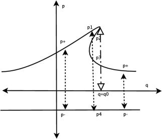
Figure 8: Fermi level

This identification with the collective field equations is perfectly fine for a fluctuation of the form shown in the figure (7). However because of the equation of the motion, points of the curve which are higher, have greater velocity than the lower points, hence even if we start with a simple profile like that given in figure (7), the profile changes due to the unequal velocity of the various points lying on the Fermi level to a profile of the form given in figure (8). In figure(8), where the profile becomes multi-valued, the identification is not as before, since there are more than two values of $p$ corresponding to the same value of $x$. For instance, if at a point the Fermi profile has a multi valuedness of the ”order four”, that is there are four values of $\hat{p}$ corresponding to the same value of $\theta$, then the equation for $\rho$ becomes

$$2\pi\rho(\theta)=\int_{\hat{p}_{3}}^{\hat{p}_{4}}dp\ {\cal U}(p,\theta)+\int_{\hat{p}_{1}}^{\hat{p}_{2}}dp\ {\cal U}(p,\theta)$$ (56)

and similarly for the equation for $\rho v$. One can easily see that one cannot derive the simple collective field equations in this case. Hence the collective field equations do not describe the dynamics of the Fermi surface at all times.

However we can still look at the the topmost value of $p$ as $\hat{p}_{+}$ and the lowest value of $p$ as $\hat{p}_{-}$. In that case the equations governing the dynamics of $p_{+}+p_{-}$ and $\hat{p}_{+}-\hat{p}_{-}$ are the same collective field equation throughout, but then we see clearly from figure (8). that the values of these variables jumps at $\theta=\theta_{0}$, and hence the $\theta$ derivative blows up at this point. This jump will correspond to the shock of the collective field equations. Note that the description in terms of the fermion phase space is always perfectly smooth since it is after all the theory of free fermions.

In our case we are dealing with a $1+1$ dimensional interacting Euclidean fermionic theory given by a Lagrangian of one fermionic field $\Psi(\theta)$

$${\cal L}=\int d\theta\Psi^{\dagger}\partial_{x}\Psi+|\partial_{\theta}\Psi|^{2}+2\xi\int d\theta d\theta^{\prime}\Psi^{\dagger}(\theta)\Psi(\theta)\cos(\theta-\theta^{\prime})\Psi^{\dagger}(\theta^{\prime})\Psi(\theta^{\prime})$$ (57)

These equations give rise to the equation of the form (14). The phase space arguments discussed here will continue to hold even in this case again leading to shock formation in finite time (see fig$.10$). But the theory viewed as a theory of fermions will still be valid.

References

- [1] E. Witten, Adv. Theor. Math. Phys. 2, 253 (1998) [arXiv:hep-th/9802150]. E. Witten, “Anti-de Sitter space, thermal phase transition, and confinement in gauge theories,” Adv. Theor. Math. Phys. 2, 505 (1998) [arXiv:hep-th/9803131].
- [2] O. Aharony, S. S. Gubser, J. M. Maldacena, H. Ooguri and Y. Oz, “Large N field theories, string theory and gravity,” Phys. Rept. 323, 183 (2000) [arXiv:hep-th/9905111].
- [3] S. J. Rey, S. Theisen and J. T. Yee, “Wilson-Polyakov loop at finite temperature in large N gauge theory and anti-de Sitter supergravity,” Nucl. Phys. B 527, 171 (1998) [arXiv:hep-th/9803135].
- [4] G. T. Horowitz and R. C. Myers, “The AdS/CFT correspondence and a new positive energy conjecture for general relativity,” Phys. Rev. D 59, 026005 (1999) [arXiv:hep-th/9808079].
- [5] J. Hallin and D. Persson, “Thermal phase transition in weakly interacting, large N(c) QCD,” Phys. Lett. B 429, 232 (1998) [arXiv:hep-ph/9803234].
- [6] B. Sundborg, “The Hagedorn transition, deconfinement and N = 4 SYM theory,” Nucl. Phys. B 573, 349 (2000) [arXiv:hep-th/9908001].
- [7] A. M. Polyakov, “Gauge fields and space-time,” Int. J. Mod. Phys. A 17S1, 119 (2002) [arXiv:hep-th/0110196].
- [8] B. Lucini, M. Teper and U. Wenger, “The deconfinement transition in SU(N) gauge theories,” Phys. Lett. B 545, 197 (2002) [arXiv:hep-lat/0206029]. B. Lucini, M. Teper and U. Wenger, JHEP 0401, 061 (2004) [arXiv:hep-lat/0307017]. B. Lucini, M. Teper and U. Wenger, “Properties of the deconfining phase transition in SU(N) gauge theories,” JHEP 0502, 033 (2005) [arXiv:hep-lat/0502003].
- [9] O. Aharony, J. Marsano, S. Minwalla, K. Papadodimas and M. Van Raamsdonk, “The Hagedorn / deconfinement phase transition in weakly coupled large N gauge theories,” Adv. Theor. Math. Phys. 8, 603 (2004) [arXiv:hep-th/0310285]. O. Aharony, J. Marsano, S. Minwalla, K. Papadodimas, M. Van Raamsdonk and T. Wiseman, “The phase structure of low dimensional large N gauge theories on tori,” JHEP 0601, 140 (2006) [arXiv:hep-th/0508077]. O. Aharony, J. Marsano, S. Minwalla and T. Wiseman, “Black hole - black string phase transitions in thermal 1+1 dimensional supersymmetric Yang-Mills theory on a circle,” Class. Quant. Grav. 21, 5169 (2004) [arXiv:hep-th/0406210]. O. Aharony, J. Marsano, S. Minwalla, K. Papadodimas and M. Van Raamsdonk, “A first order deconfinement transition in large N Yang-Mills theory on a small S**3,” Phys. Rev. D 71, 125018 (2005) [arXiv:hep-th/0502149].
- [10] H. J. Schnitzer, “Confinement / deconfinement transition of large N gauge theories with N(f) Nucl. Phys. B 695, 267 (2004) [arXiv:hep-th/0402219].
- [11] M. Spradlin and A. Volovich, “A pendant for Polya: The one-loop partition function of N = 4 SYM on R x Nucl. Phys. B 711, 199 (2005) [arXiv:hep-th/0408178].
- [12] L. Alvarez-Gaume, C. Gomez, H. Liu and S. Wadia, “Finite temperature effective action, AdS(5) black holes, and 1/N expansion,” Phys. Rev. D 71, 124023 (2005) [arXiv:hep-th/0502227].
- [13] P. Basu and S. R. Wadia, “R-charged AdS(5) black holes and large N unitary matrix models,” Phys. Rev. D 73, 045022 (2006) [arXiv:hep-th/0506203].
- [14] O. Aharony, S. Minwalla and T. Wiseman, “Plasma-balls in large N gauge theories and localized black holes,” Class. Quant. Grav. 23, 2171 (2006) [arXiv:hep-th/0507219].
- [15] L. Alvarez-Gaume, P. Basu, M. Marino and S. R. Wadia, “Blackhole / string transition for the small Schwarzschild blackhole of AdS(5) x S**5 and critical unitary matrix models,” arXiv:hep-th/0605041.
- [16] V. E. Hubeny and M. Rangamani, “Unstable horizons,” JHEP 0205, 027 (2002) [arXiv:hep-th/0202189].
- [17] J. M. Maldacena, “Eternal black holes in Anti-de-Sitter,” JHEP 0304, 021 (2003) [arXiv:hep-th/0106112].
- [18] P. Kraus, H. Ooguri and S. Shenker, “Inside the horizon with AdS/CFT,” Phys. Rev. D 67, 124022 (2003) [arXiv:hep-th/0212277].
- [19] L. Fidkowski, V. Hubeny, M. Kleban and S. Shenker, “The black hole singularity in AdS/CFT,” JHEP 0402, 014 (2004) [arXiv:hep-th/0306170].
- [20] H. Liu, “Fine structure of Hagedorn transitions,” [arXiv:hep-th/0408001]
- [21] G. Festuccia and H. Liu, “Excursions beyond the horizon: Black hole singularities in Yang-Mills theories. I,” JHEP 0604, 044 (2006) [arXiv:hep-th/0506202].
- [22] S. J. Rey and Y. Hikida, “5d black hole as emergent geometry of weakly interacting 4d hot Yang-Mills gas,” JHEP 0608, 051 (2006) [arXiv:hep-th/0507082].
- [23] S. Kalyana Rama and B. Sathiapalan, “The Hagedorn transition, deconfinement and the AdS/CFT correspondence,” Mod. Phys. Lett. A 13, 3137 (1998) [arXiv:hep-th/9810069]. S. Kalyana Rama and B. Sathiapalan, “On the role of chaos in the AdS/CFT connection,” Mod. Phys. Lett. A 14, 2635 (1999) [arXiv:hep-th/9905219].
- [24] D. Yamada and L. G. Yaffe, “Phase diagram of N = 4 super-Yang-Mills theory with R-symmetry chemical potentials,” JHEP 0609, 027 (2006) [arXiv:hep-th/0602074].
- [25] H. Nastase, “The RHIC fireball as a dual black hole,” arXiv:hep-th/0501068. H. Nastase, “More on the RHIC fireball and dual black holes,” arXiv:hep-th/0603176.
- [26] T. Hollowood, S. P. Kumar and A. Naqvi, “Instabilities of the small black hole: A view from N = 4 SYM,” arXiv:hep-th/0607111.
- [27] J. R. David, G. Mandal and S. R. Wadia, “Microscopic formulation of black holes in string theory,” Phys. Rept. 369, 549 (2002) [arXiv:hep-th/0203048].
- [28] E. Brezin, C. Itzykson, G. Parisi and J. B. Zuber, “Planar Diagrams,” Commun. Math. Phys. 59, 35 (1978).
- [29] D. J. Gross and E. Witten, “Possible Third Order Phase Transition In The Large N Lattice Gauge Theory,” Phys. Rev. D 21, 446 (1980).
- [30] S. R. Wadia, “N = Infinity Phase Transition In A Class Of Exactly Soluble Model Lattice Gauge Theories,” Phys. Lett. B 93, 403 (1980). S. Wadia, “A Study Of U(N) Lattice Gauge Theory In Two-Dimensions,” EFI-79/44-CHICAGO
- [31] A. M. Sengupta and S. R. Wadia, “Excitations And Interactions In D = 1 String Theory,” Int. J. Mod. Phys. A 6, 1961 (1991).
- [32] D. J. Gross and I. R. Klebanov, “Fermionic string field theory of c = 1 two-dimensional quantum gravity,” Nucl. Phys. B 352, 671 (1991).
- [33] J. Polchinski, “Classical Limit Of (1+1)-Dimensional String Theory,” Nucl. Phys. B 362, 125 (1991).
- [34] A. Dhar, G. Mandal and S. R. Wadia, “Classical Fermi Fluid And Geometric Action For C=1,” Int. J. Mod. Phys. A 8, 325 (1993) [arXiv:hep-th/9204028].
- [35] A. Dhar, G. Mandal and S. R. Wadia, “Nonrelativistic fermions, coadjoint orbits of W(infinity) and string field theory at c = 1,” Mod. Phys. Lett. A 7, 3129 (1992) [arXiv:hep-th/9207011].
- [36] A. Jevicki and B. Sakita, “The quantum collective field method and its application to the planar limit,” Nucl. Phys. B 165, 511 (1980).
- [37] G. K. Savvidy, “Infrared Instability Of The Vacuum State Of Gauge Theories And Asymptotic Freedom,” Phys. Lett. B 71, 133 (1977).
- [38] G. W. Semenoff, O. Tirkkonen and K. Zarembo, “Exact solution of the one-dimensional non-Abelian Coulomb gas at large N,” Phys. Rev. Lett. 77, 2174 (1996) [arXiv:hep-th/9605172].
- [39] P. M. Chaikin, T. C. Lubensky ”Principles of Condensed Matter Physics” Cambridge University Press, 1998
- [40] R. Rajaraman ”Solitons and Instantons” North-Holland Publishing Company, 1982
- [41] D. Chae, A. Cordoba, D. Cordoba, M.A. Fontelos ”Finite time singularities in a 1D model of the quasi-geostropic equation” (To Appear in Advances in Mathematics)