The Four-Loop Planar Amplitude and Cusp Anomalous Dimension in Maximally Supersymmetric Yang-Mills Theory

Abstract

We present an expression for the leading-color (planar) four-loop four-point amplitude of ${\cal N}=4$ supersymmetric Yang-Mills theory in $4-2\epsilon$ dimensions, in terms of eight separate integrals. The expression is based on consistency of unitarity cuts and infrared divergences. We expand the integrals around $\epsilon=0$, and obtain analytic expressions for the poles from $1/\epsilon^{8}$ through $1/\epsilon^{4}$. We give numerical results for the coefficients of the $1/\epsilon^{3}$ and $1/\epsilon^{2}$ poles. These results all match the known exponentiated structure of the infrared divergences, at four separate kinematic points. The value of the $1/\epsilon^{2}$ coefficient allows us to test a conjecture of Eden and Staudacher for the four-loop cusp (soft) anomalous dimension. We find that the conjecture is incorrect, although our numerical results suggest that a simple modification of the expression, flipping the sign of the term containing $\zeta_{3}^{2}$, may yield the correct answer. Our numerical value can be used, in a scheme proposed by Kotikov, Lipatov and Velizhanin, to estimate the two constants in the strong-coupling expansion of the cusp anomalous dimension that are known from string theory. The estimate works to 2.6% and 5% accuracy, providing non-trivial evidence in support of the AdS/CFT correspondence. We also use the known constants in the strong-coupling expansion as additional input to provide approximations to the cusp anomalous dimension which should be accurate to under one percent for all values of the coupling. When the evaluations of the integrals are completed through the finite terms, it will be possible to test the iterative, exponentiated structure of the finite terms in the four-loop four-point amplitude, which was uncovered earlier at two and three loops.

I Introduction

Maximally supersymmetric ${\cal N}=4$ Yang-Mills theory (MSYM) has attracted a great deal of theoretical interest over the years. It is widely believed that the ’t Hooft (planar) limit of MSYM, in which the number of colors $N_{c}$ is taken to infinity, is dual at strong coupling ($\lambda\equiv g^{2}N_{c}\to\infty$) to weakly-coupled gravity in five-dimensional anti-de Sitter space Maldacena . The duality implies that the full quantum anomalous dimensions of various series of gauge-invariant composite operators are equal to energies of different gravity modes or configurations of strings in anti-de Sitter space BPS ; OtherAnomalousDim ; BMN ; Nontrivial ; DhokerTasi . Heuristically, the Maldacena duality conjecture hints that even quantities unprotected by supersymmetry should have perturbative series that can be resummed in closed form. The strong-coupling limits of these resummed expressions, possibly supplemented by non-perturbative contributions, should match results for the appropriate observables in weakly-coupled supergravity or string theory.

This intuition does appear to apply to the higher-loop on-shell scattering amplitudes of color-non-singlet gluons, even though the Maldacena conjecture does not directly address on-shell amplitudes of massless colored quanta. There is now significant evidence of a very simple structure in the planar limit. In particular, the planar contributions to the two-loop and three-loop four-gluon amplitudes have been shown to obey iterative relations Iterate2 ; Iterate3 : The dimensionally regularized amplitudes ($d=4-2\epsilon$) can be expressed in terms of lower-loop amplitudes, along with a set of three constants for each order in the loop expansion.

An analogous relation is conjectured to hold for generic maximally-helicity-violating (MHV) $n$-gluon scattering amplitudes, to all loop orders Iterate2 ; Iterate3 . The MHV amplitudes are those for which two of the gluons have negative helicity and the remaining $(n-2)$ have positive helicity, or the parity conjugate case. Indirect evidence for the extension to the $n$-point MHV case was provided first by studying the consistency of collinear limits at two loops Iterate2 . Later, the iteration relation was demonstrated to hold directly for the two-loop five-gluon amplitude, for the “even” terms in the amplitude CSV06 and soon thereafter for the “odd” terms as well, i.e. for the complete amplitude BCKRS . (Odd and even refer to the behavior of the ratio of terms in the loop amplitude to the tree amplitude, under parity.) After infrared divergences have been subtracted from the proposed all-loop iterative relation, the resulting finite remainder is neatly proportional to an exponential of the product of the one-loop finite remainder with the so-called cusp anomalous dimension. Presumably the weak–strong duality between anti-de Sitter space and conformal field theory (AdS/CFT) plays a role in this simplicity.

The form of the proposed iterative structure of multi-loop planar MSYM is based on the understanding of how soft and collinear infrared singularities factorize and exponentiate in gauge theory Akhoury ; Sudakov ; Sen83 ; SoftGluonSummation ; MagneaSterman ; IROneLoop ; CataniIR ; TYS . For the pole terms in the amplitudes, such behavior is universal, and holds in any massless gauge theory. What is remarkable in planar MSYM is that the finite terms in the MHV scattering amplitudes can be organized into the same exponentiated form as the divergent terms. In a non-supersymmetric theory, QCD, exponentiation of finite terms has also been observed in the context of threshold resummation of the Drell-Yan cross section EynckLaenenMagnea . In the case of four-gluon amplitudes in MSYM, the behavior is valid for arbitrary values of the scattering angle (ratio of $t/s$). For amplitudes with more than four gluons, there are many kinematical variables, and so the constraints imposed by the iterative structure are even stronger. It is clearly of interest to test whether this structure persists beyond three loops. In this paper we shall provide an integral representation for the planar four-loop four-gluon amplitude. Our result will enable such a test to be performed at four loops, once the relevant integrals have been evaluated to sufficiently high order in $\epsilon$.

Another remarkable property of planar MSYM is the integrability of the dilatation operator, interpreted as a Hamiltonian, for many sectors of the theory. Integrable structures were identified in anomalous dimension matrices in QCD a while ago QCDIntegrable . In planar MSYM, Minahan and Zarembo MinahanZarembo mapped the one-loop dilatation operator for non-derivative single-trace operators to an integrable spin-chain Hamiltonian, and used a Bethe ansatz to compute the anomalous dimensions. Such integrable structures have since been extended to higher perturbative orders for various sectors of the theory MoreIntegrable ; BeisertDispersion ; Integrable . They are also known to be present at strong coupling, from the form of the classical sigma model on target space AdS${}_{5}\times S^{5}$ BPR . (Berkovits has given a formal argument that the integrability extends to the quantum level on the world sheet Berkovits .) The iterative structure of MSYM amplitudes may somehow be related to integrability. If an infinite number of conserved charges are present, the form of the quantum corrections should be severely constrained, as it would be by the proposed iterative structure Iterate2 ; Iterate3 . An iterative structure may also arise in correlation functions of gauge-invariant composite operators in planar MSYM Schubert ; but its precise structure, if it exists in this context, has not yet been clarified.

Integrability is a powerful computational tool. Integrability, or in some cases, the assumption of integrability, has been employed to compute a variety of one-loop and multi-loop anomalous dimensions in planar MSYM from Bethe ansätze MinahanZarembo ; MoreIntegrable ; BeisertDispersion and from the Baxter equation BGK06 ; Belitsky . One of the most interesting developments along these lines has been the all-orders proposal of Eden and Staudacher (ES), based on an asymptotic all-loop Bethe ansatz AsymptoticBA , for the large-spin limit of the anomalous dimensions of leading-twist operators in MSYM EdenStaudacher . This quantity, $\gamma_{K}(\alpha_{s})$, is also referred to as the cusp (or sometimes, soft) anomalous dimension associated with a Wilson line. Equivalently, it represents the leading large-$x$ behavior KM of the DGLAP kernel $P_{ii}(x)$ for parton evolution, $i\to i$,

$$P_{ii}(x)\to{\gamma_{K}(\alpha_{s})\over 2\,(1-x)_{+}}+B(\alpha_{s})\,\delta(1-x)+\ldots,\qquad{\rm as}\ \ x\to 1.$$ (1)

Taking Mellin moments, $\gamma(j)\equiv-\int_{0}^{1}dx\,x^{j-1}P(x)$, we see that the cusp anomalous dimension gives the dominant behavior of the leading-twist anomalous dimensions as the spin $j\to\infty$,

$$\gamma(j)={1\over 2}\gamma_{K}(\alpha_{s})\ \ln(j)+{\cal O}(j^{0})\,.$$ (2)

From the asymptotic all-loop Bethe ansatz, ES derived an integral equation for a fluctuation density $\hat{\sigma}$, from which the cusp anomalous dimension can be determined. The integral equation is straightforward to solve perturbatively in $\alpha_{s}$. In terms of the expansion parameter

$$\hat{a}\equiv{g^{2}N_{c}\over 8\pi^{2}}={N_{c}\alpha_{s}\over 2\pi}\,,$$ (3)

the ES prediction for (one quarter of) the cusp anomalous dimension is EdenStaudacher

$${\gamma_{K}(\hat{a})\over 4} \equiv f_{0}(\hat{a})$$ (6)

$$= \hat{a}-\zeta_{2}\,\hat{a}^{2}+\Bigl{(}\zeta_{2}^{2}+3\,\zeta_{4}\Bigr{)}\hat{a}^{3}$$

$$\hskip 0.0pt\hbox{}-\Bigl{(}\zeta_{2}^{3}+6\,\zeta_{2}\,\zeta_{4}-\zeta_{3}^{2}+{25\over 2}\,\zeta_{6}\Bigr{)}\hat{a}^{4}$$

$$\hskip 0.0pt\hbox{}+\Bigl{(}\zeta_{2}^{4}+9\,\zeta_{2}^{2}\,\zeta_{4}-2\,\zeta_{2}\,\zeta_{3}^{2}+25\,\zeta_{2}\,\zeta_{6}-10\,\zeta_{3}\,\zeta_{5}+{39\over 4}\,\zeta_{4}^{2}+{245\over 4}\,\zeta_{8}\Bigr{)}\hat{a}^{5}\ +\ \cdots~{}~{}~{}~{}~{}~{}$$

$$= \hat{a}-{\pi^{2}\over 6}\,\hat{a}^{2}+{11\over 180}\pi^{4}\,\hat{a}^{3}-\Bigl{(}{73\over 2520}\,\pi^{6}-\zeta_{3}^{2}\Bigr{)}\hat{a}^{4}$$

$$\hskip 0.0pt\hbox{}+\Bigl{(}{887\over 56700}\,\pi^{8}-{\pi^{2}\over 3}\,\zeta_{3}^{2}-10\,\zeta_{3}\,\zeta_{5}\Bigr{)}\hat{a}^{5}+\ \cdots\,.$$

Here $f_{0}(\hat{a})$ can be identified with the first of a series of three constants (per loop order) appearing in the iterative relation for the four-gluon amplitude Iterate2 ; Iterate3 . The first three terms of eq. (6) agree with previously-known results Makeenko ; KLV ; KLOV ; Iterate3 ; MOS , so the new predictions begin with the $\hat{a}^{4}$ term. The conjecture (6) has also been arrived at recently by Belitsky, using a proposed generalization of the Baxter equation to all loop orders Belitsky .

In QCD the three-loop cusp (soft) anomalous dimension has been computed by Moch, Vermaseren and Vogt as part of the impressive computation of the full leading-twist anomalous dimensions MVV needed for next-to-next-to-leading order evolution of parton distribution functions. (Terms proportional to the number of quark flavors were obtained first in ref. SoftNf .) Kotikov, Lipatov, Onishchenko and Velizhanin (KLOV) KLOV made the inspired observation, based on evidence at two loops KL02 , that the MSYM anomalous dimensions may be obtained simply from the “leading-transcendentality” contributions in QCD. The cusp anomalous dimensions are polynomials in the Riemann $\zeta$ values, $\zeta_{n}\equiv\zeta(n)$, or their multi-index generalizations, $\zeta_{n_{1},n_{2},\ldots}$. (These cannot show up below five loops.) The degree of transcendentality of $\zeta_{n}$ is just $n$, and the transcendentality is additive for products of $\zeta$ values. At $L$ loops, the leading-transcendentality contributions to the cusp anomalous dimension have degree (or weight) equal to $2L-2$. All MSYM leading-twist anomalous dimensions computed to date have had uniform, leading transcendentality, whereas the corresponding QCD results contain an array of terms of lower transcendentality, all the way down to rational numbers.

The KLOV conversion principle applies to the leading-twist anomalous dimensions for any spin $j$, with an appropriate definition of leading transcendentality for the harmonic sums $S_{\vec{m}}(j)$ that appear in the results. Using assumptions of integrability, Staudacher confirmed the three-loop KLOV result through $j=70$ Staudacher ; StaudacherPrivate , building on earlier work of Beisert, Kristjansen and Staudacher MoreIntegrable at $j=4$. Eden and Staudacher extended this analysis to the three-loop cusp anomalous dimension (the $j\to\infty$ limit), in the course of arriving at their all-orders proposal (6) based on integrability EdenStaudacher . The three-loop cusp anomalous dimension in MSYM was independently determined from the $1/\epsilon^{2}$ pole in the three-loop four-gluon scattering amplitude Iterate3 , providing a confirmation of the KLOV result in the limit $j\to\infty$. An important feature of the ES proposal (6) is that it is consistent with KLOV’s observation that the MSYM anomalous dimensions are homogeneous in the transcendentality, at least through three loops.

The ES proposal emerges from mapping single-trace gauge-invariant operators to spin chains. The dilatation operator, whose eigenvalues are anomalous dimensions, is mapped to the spin-chain Hamiltonian. The form of the $S$ matrix for this spin chain is fixed, up to an overall phase, called the dressing factor AFS04 , by the superconformal [PSU$(2,2|4)$] symmetry of both AdS${}_{5}\times S^{5}$ and ${\cal N}=4$ supersymmetric gauge theory. At one and two loops, superconformal symmetry in combination with explicit calculations fixes the dressing factor to be 1. At higher loops, it is not so constrained. A nontrivial dressing factor is required by the strong-coupling behavior AFS04 ; OtherDressing ; HernandezLopez , and there have been several recent investigations of it using properties such as worldsheet crossing symmetry JanikCrossing ; BHL . Yet the order in the weak-coupling expansion at which it becomes nontrivial is still uncertain.

The presence of a dressing factor at three loops would lead to a shift in the anomalous dimension at four loops. For example, ES have proposed EdenStaudacher a modification of the asymptotic Bethe ansatz AsymptoticBA at this order, with coefficient $\beta$, which is consistent with the presently known integrable structure. This modification alters the predicted four-loop anomalous dimension in eq. (6) to

$$-\Bigl{(}{73\over 2520}\,\pi^{6}-\zeta_{3}^{2}+2\beta\zeta_{3}\Bigr{)}\hat{a}^{4}\,.$$ (7)

Thus a calculation of the four-loop cusp anomalous dimension has the potential to probe a nontrivial dressing factor. In a new preprint BESNew , Beisert, Eden and Staudacher (BES) have shown how to extend the above dressing factor to all orders in the coupling, as well as to ensure its consistency with other constraints. This leads to the prediction that $\beta=\zeta_{3}$.

In this paper, we perform this calculation, in order to test whether the ES all-orders proposal gives the correct result, or to reveal how it needs to be modified if it doesn’t. We do so by evaluating the infrared poles of the planar four-loop four-gluon scattering amplitude through $1/\epsilon^{2}$, the order at which the four-loop cusp anomalous dimension appears. The form of the infrared singularities at all loop orders are fully understood MagneaSterman , up to a set of constants that must be computed explicitly. At $1/\epsilon^{2}$ this undetermined constant is precisely the cusp anomalous dimension appearing in the ES formula.

First, though, we need a representation of the planar four-loop four-gluon amplitude. Rather than construct this representation from Feynman diagrams, we shall employ the unitarity method NeqFourOneLoop ; Fusing ; UnitarityMachinery ; OneLoopReview ; TwoLoopSplitting . This method was also used to construct the planar two- and three-loop amplitudes BRY ; Iterate3 . Because the unitarity method builds amplitudes at any loop order from on-shell lower-loop amplitudes, structure uncovered at the tree and one-loop levels can easily be fed back into the construction of the higher-loop amplitudes. We will find that the planar four-loop amplitude can be expressed as a linear combination of just eight four-loop integrals.

A very interesting feature of the integrals appearing in the planar four-point amplitudes through four loops is that they are all, in a well-defined sense, conformally invariant. To analyze the conformal properties of potential four-loop integrals, we make use of the recent description of such integrals by Drummond, Henn, Sokatchev, and one of the authors DHSS .

Once we know what four-loop four-point integrals enter into the amplitude, we must compute them explicitly through ${\cal O}(\epsilon^{-2})$. Here we make use of important recent advances in multi-loop integration SmirnovDoubleBox ; LoopIntegrationAdvance ; SmirnovTripleBox ; Tausk ; TwoloopOffandMassive ; Buch ; AnastasiouDaleo ; CzakonMB . In particular, we use the program MB CzakonMB to automatically extract poles in $\epsilon$ from the Mellin-Barnes representation of loop integrals, and to integrate the resulting contour integrals. We carry out the integrations analytically for coefficients of the first five poles, $1/\epsilon^{8}$ through $1/\epsilon^{4}$. These coefficients are expressed in terms of well-studied functions, harmonic polylogarithms (HPLs) HPL ; HPL2 , making it straightforward to confirm the expected infrared structure for arbitrary values of the scattering angle. For the coefficients of the $1/\epsilon^{3}$ and $1/\epsilon^{2}$ poles, our analysis is numerical. We evaluate the amplitude at four kinematic points, $(s,t)=(-1,-1)$, $(-1,-2)$, $(-1,-3)$, and $(-1,-15)$. Numerical evaluation suffices because the expected behavior is completely specified at order $1/\epsilon^{3}$, and specified up to one unknown, but predicted, constant, $f_{0}^{(4)}$, at order $1/\epsilon^{2}$. We find consistent results from all four kinematic points.

We also need to evaluate the infrared singular terms to the same order $1/\epsilon^{2}$. These may be expressed in terms of lower-loop amplitudes. For this purpose, we must expand the one-, two-, and three-loop amplitudes to ${\cal O}(\epsilon^{4})$, ${\cal O}(\epsilon^{2})$ and ${\cal O}(\epsilon^{0})$, respectively. Fortunately, these are precisely the orders required to test the full iteration relation at three loops, so the needed lower-loop expressions can all be found, in analytic form, in ref. Iterate3 . (These results are based partly on the earlier evaluation of the double-box SmirnovDoubleBox and triple-ladder SmirnovTripleBox integrals.)

We find that the ES conjecture is incorrect, although our numerical results suggest that a simple modification of the four-loop ES prediction may yield the correct answer. In particular, if we flip the sign of the $\zeta_{3}^{2}$ term in their prediction, we obtain a value within the error bars of our result. If we choose to interpret the modification as a dressing factor within the form taken in ref. EdenStaudacher , it suggests taking the value $\beta=\zeta_{3}$ for their parameter. This value would violate the apparent “uniform transcendentality” observed to date generally for quantities in the ${\cal N}=4$ theory, for example in the anomalous dimension of the higher-twist operator $\,{\rm Tr}(X^{2}Z^{3})+\cdots$ EdenStaudacher . The same value, $\beta=\zeta_{3}$, was suggested independently by BES BESNew , based on properties of the spin-chain model. This coincidence, modulo caveats we shall discuss in section VII, provides some support to violation of uniform transcendentality in quantities other than the cusp anomalous dimension. This possibility can be tested via other perturbative computations; if uniform transcendentality is nonetheless maintained, our result might instead imply that the form postulated for the dressing factor in ES and elsewhere AFS04 ; OtherDressing ; BeisertKlose ; BeisertInvariant ; BeisertDynamic ; BeisertPhase ; BHL is not general enough.

We also use our four-loop results to investigate the strong-coupling limit of the cusp anomalous dimension. In the AdS/CFT correspondence, this quantity can be computed from the energy of a long, folded string, spinning in AdS₅ StrongCouplingLeadingGKP . The first two coefficients in the strong-coupling, large-$N_{c}$ limit of the cusp anomalous dimension have been determined using a semi-classical expansion based on this string configuration StrongCouplingLeadingGKP ; Kruczenski ; Makeenko ; StrongCouplingSubleading . We shall discuss how our four-loop result can be used to give a remarkably accurate estimate for these coefficients. We employ an approximate formula devised by Kotikov, Lipatov and Velizhanin KLV ; KLOV to interpolate between the weak- and strong-coupling regimes. Using our four-loop result as input to this formula, the first two strong-coupling coefficients are estimated to within 2.6% and 5%, respectively, of the values computed from string theory. This agreement provides direct evidence in support of the AdS/CFT correspondence as well as a smooth transition between weak and strong coupling.

An even better approximation for the cusp anomalous dimension can be found by incorporating into the interpolating formula the string predictions for the first two coefficients in the strong-coupling expansion. Based on our success in accurately estimating the two leading strong-coupling coefficients, we expect this improved approximation to be accurate to within a few percent, for all values of the coupling. Curiously, our approximate formula predicts that the third coefficient in the strong-coupling expansion should be very small, and may even vanish. The formula also predicts the numerical value of the five-loop coefficient. This value turns out to be extremely close to a simple modification of the five-loop ES prediction, flipping the signs of the terms containing odd $\zeta$ values, as at four loops. We have confirmed our analysis using Padé approximants, which also give insight into the complex analytic structure of $f_{0}(\hat{a})$.

Our representation of the planar four-loop four-gluon amplitude in terms of eight four-loop integrals can be used for more than just the extraction of the cusp anomalous dimension. As mentioned above, it can also be used to check the proposed iterative structure at four loops. In order to do so, one would need to evaluate the integrals all the way through the finite terms, ${\cal O}(\epsilon^{0})$, instead of just the level carried out in this paper, ${\cal O}(\epsilon^{-2})$. One would also need to evaluate all integrals appearing in the lower-loop amplitudes to two orders higher in $\epsilon$.

This paper is organized as follows. In section II, we review the iterative structure of MSYM loop amplitudes, commenting in particular on how the cusp anomalous dimension appears in the infrared singular terms. In section III, we present the construction of the four-loop amplitudes via the unitarity method and also describe the conformal properties of the resulting integrals. In section IV, we give analytical results for the amplitudes through ${\cal O}(\epsilon^{-4})$ and numerical results though ${\cal O}(\epsilon^{-2})$, allowing us to extract a numerical value for the four-loop cusp anomalous dimension. The four-loop anomalous dimension is then used in section VII to estimate the coefficients that appear at strong coupling and also to estimate higher-loop contributions to the cusp anomalous dimension. Our conclusions are given in section VIII. Two appendices are included, one presenting Mellin-Barnes representations for the integrals appearing in the four-loop amplitude, and one reviewing properties of harmonic polylogarithms.

II Iterative structure of MSYM loop amplitudes

In this paper we consider the planar contributions to gluonic scattering in MSYM with gauge group $SU(N_{c})$, that is, the leading terms as $N_{c}\to\infty$. We do not discuss subleading-color contributions; at present they do not appear to have a simple iterative structure Iterate2 .

The leading-color terms have the same color structure as the corresponding tree amplitudes. The leading-$N_{c}$ contributions to the $L$-loop $SU(N_{c})$ gauge-theory $n$-point amplitudes may be written as,

$${\cal A}_{n}^{(L)} = g^{n-2}\Biggl{[}{2e^{-\epsilon\gamma}g^{2}N_{c}\over(4\pi)^{2-\epsilon}}\Biggr{]}^{L}\sum_{\sigma\in S_{n}/Z_{n}}\,{\rm Tr}(T^{a_{\sigma(1)}}\ldots T^{a_{\sigma(n)}})A_{n}^{(L)}(\sigma(1),\sigma(2),\ldots,\sigma(n))\,,$$ (8)

where $\gamma$ is Euler’s constant, and the sum runs over non-cyclic permutations of the external legs. In this expression we have suppressed the (all-outgoing) momenta $k_{i}$ and helicities $\lambda_{i}$, leaving only the index $i$ as a label. This decomposition holds for all particles in the gauge super-multiplet, as they are all in the adjoint representation. The color-ordered partial amplitudes $A_{n}$ are independent of the color factors, and depend only on the kinematics. For MSYM, supersymmetric Ward identities SWI imply that the four-gluon helicity amplitudes $({+}{+}{+}{+})$ and $({-}{+}{+}{+})$ (as well as their parity conjugates) vanish identically. Furthermore, the nonvanishing four-point (MHV) amplitudes are all related by simple overall factors. Hence we do not need to specify the helicity configuration, i.e. whether the color ordering is $({-}{-}{+}{+})$ or $({-}{+}{-}{+})$.

It is convenient to scale out a factor of the tree amplitude, and work with the quantities $M_{n}^{(L)}$ defined by

$$M_{n}^{(L)}(\rho;\epsilon)=A_{n}^{(L)}(\rho)/A_{n}^{(0)}(\rho)\,.$$ (9)

Here $\rho$ indicates the dependence on the external momenta, $\rho\equiv\{s_{12},s_{23},\ldots\}$, where $s_{i(i+1)}=(k_{i}+k_{i+1})^{2}$ are invariants built from color-adjacent momenta. The iteration relation proposed in ref. Iterate3 then takes the form,

$${\cal M}_{n}(\rho)\equiv 1+\sum_{L=1}^{\infty}a^{L}M_{n}^{(L)}(\rho;\epsilon)=\exp\Biggl{[}\sum_{l=1}^{\infty}a^{l}\Bigl{(}f^{(l)}(\epsilon)M_{n}^{(1)}(\rho;l\epsilon)+C^{(l)}+E_{n}^{(l)}(\rho;\epsilon)\Bigr{)}\Biggr{]}\,.$$ (10)

In this expression, the factor,

$$a\equiv{N_{c}\alpha_{s}\over 2\pi}(4\pi e^{-\gamma})^{\epsilon}\,,$$ (11)

keeps track of the loop order of perturbation theory, and coincides with the prefactor in brackets in eq. (8). (It becomes equal to $\hat{a}$ in eq. (3) as $\epsilon\to 0$.) The quantity $M_{n}^{(1)}(\rho;l\epsilon)$ is the one-loop amplitude, with the tree amplitude scaled out according to eq. (9), and with the substitution $\epsilon\to l\epsilon$ performed. (That is, it is evaluated in $d=4-2l\epsilon$.) Each $f^{(l)}(\epsilon)$ is given by a three-term series in $\epsilon$, beginning at ${\cal O}(\epsilon^{0})$,

$$f^{(l)}(\epsilon)=f_{0}^{(l)}+\epsilon f_{1}^{(l)}+\epsilon^{2}f_{2}^{(l)}\,.$$ (12)

The objects $f_{k}^{(l)}$, $k=0,1,2$, and $C^{(l)}$ are pure constants, independent of the external kinematics $\rho$, and also independent of the number of legs $n$. We expect them to be polynomials in the Riemann values $\zeta_{m}$ with rational coefficients, and a uniform degree of transcendentality, which is equal to $2l-2+k$ for $f_{k}^{(l)}$, and $2l$ for $C^{(l)}$. (Multiple zeta values $\zeta_{n_{1},n_{2},\ldots}$ may also appear, but there are no independent ones of weight less than eight, and so they can only appear starting at five-loop order.) The $f_{k}^{(l)}$ and $C^{(l)}$ can be determined by matching to explicit computations. The one-loop values are defined to be,

$$f^{(1)}(\epsilon)=1\,,\hskip 56.9055ptC^{(1)}=0\,,\hskip 56.9055ptE_{n}^{(1)}(\rho;\epsilon)=0\,.$$ (13)

The $E_{n}^{(l)}(\rho;\epsilon)$ are non-iterating ${\cal O}(\epsilon)$ contributions to the $l$-loop amplitudes, which vanish as $\epsilon\rightarrow 0$, $E_{n}^{(l)}(\rho;0)=0$. These terms contribute to the exponentiated form of the amplitudes (10) even for $\epsilon\rightarrow 0$ because they can appear multiplied by the infrared-divergent parts of the one-loop amplitude $M_{n}^{(1)}(\rho;l\epsilon)$. After canceling the infrared divergences between real emission and virtual contributions, such terms should not contribute to infrared-safe observables.

The first two values of $f^{(l)}(\epsilon)$ in the three-term expansion (12), namely $f^{(l)}_{0}$ and $f^{(l)}_{1}$, can be identified with quantities appearing in the resummed Sudakov form factor MagneaSterman ,

$$f^{(l)}_{0} = {1\over 4}\,\hat{\gamma}_{K}^{(l)}\,,$$ (14)

$$f^{(l)}_{1} = {l\over 2}\,\hat{\cal G}_{0}^{(l)}\,.$$ (15)

The first object, $f^{(l)}_{0}$, is identified with the $l$-loop cusp anomalous dimension. The quantities $f^{(l)}_{0}$ and $\hat{\cal G}_{0}^{(l)}=(2/l)f^{(l)}_{1}$ are known through three loops KL02 ; Makeenko ; KLV ; KLOV ; Iterate3 ; MOS ,

$$f_{0}^{(1)} = 1\,,$$

$$f_{0}^{(2)} = -\zeta_{2}\,,$$ (16)

$$f_{0}^{(3)} = {11\over 2}\zeta_{4}$$

(see also eq. (6)), and

$$\hat{\cal G}_{0}^{(1)} = 0\,,$$

$$\hat{\cal G}_{0}^{(2)} = -\zeta_{3}\,,$$ (17)

$$\hat{\cal G}_{0}^{(3)} = 4\zeta_{5}+{10\over 3}\zeta_{2}\zeta_{3}\,.$$

A principal task of this paper is to compute $f_{0}^{(4)}$ and compare the result with the prediction (6).

Equation (10) is equivalent Iterate3 to

$$M_{n}^{(L)}(\rho;\epsilon)=X_{n}^{(L)}\bigl{[}M_{n}^{(l)}(\rho;\epsilon)\bigr{]}+f^{(L)}(\epsilon)M_{n}^{(1)}(\rho;L\epsilon)+C^{(L)}+E_{n}^{(L)}(\rho;\epsilon)\,,$$ (18)

where the quantities $X_{n}^{(L)}=X_{n}^{(L)}[M_{n}^{(l)}]$ only depend on the lower-loop amplitudes $M_{n}^{(l)}(\rho;\epsilon)$ with $l<L$. The $X_{n}^{(L)}$ can be computed simply by performing the following Taylor expansion,

$$X_{n}^{(L)}\bigl{[}M_{n}^{(l)}\bigr{]}=M_{n}^{(L)}-\ln\Biggl{(}1+\sum_{l=1}^{\infty}a^{l}M_{n}^{(l)}\Biggr{)}\Biggr{|}_{a^{L}\ {\rm term}}\,.$$ (19)

Eqs. (18) and (19) express the $L$-loop amplitude explicitly in terms of lower-loop amplitudes, plus constant remainders. Here we need the values of $X_{n}^{(L)}$ for $L=2,3,4$,

$$X_{n}^{(2)}\bigl{[}M_{n}^{(l)}\bigr{]} = {1\over 2}\Bigl{[}M_{n}^{(1)}\Bigr{]}^{2}\,,$$ (20)

$$X_{n}^{(3)}\bigl{[}M_{n}^{(l)}\bigr{]} = -{1\over 3}\Bigl{[}M_{n}^{(1)}\Bigr{]}^{3}+M_{n}^{(1)}M_{n}^{(2)}\,,$$ (21)

$$X_{n}^{(4)}\bigl{[}M_{n}^{(l)}\bigr{]} = {1\over 4}\Bigl{[}M_{n}^{(1)}\Bigr{]}^{4}-\Bigl{[}M_{n}^{(1)}\Bigr{]}^{2}M_{n}^{(2)}+M_{n}^{(1)}M_{n}^{(3)}+{1\over 2}\Bigl{[}M_{n}^{(2)}\Bigr{]}^{2}\,.$$ (22)

We note that the exponentiated result (10) leads to a simple exponentiated form for suitably-defined “finite remainders” $F_{n}^{(L)}$ associated with the multi-loop amplitudes Iterate3 . We define

$$F_{n}^{(L)}(\rho;\epsilon)=M_{n}^{(L)}-\sum_{l=0}^{L-1}\hat{I}_{n}^{(L-l)}\,M_{n}^{(l)}\,,$$ (23)

where the $\hat{I}_{n}^{(L-l)}(\rho;\epsilon)$ are iteratively-defined divergent terms, and $M_{n}^{(0)}\equiv 1$. After some algebra, one finds that $I_{n}^{(L)}(\rho;\epsilon)$ and $F_{n}^{(L)}(\rho;\epsilon)$ obey iterative relations very similar to eq. (18). In the limit as $\epsilon\to 0$, the relation for $F_{n}^{(L)}(\rho;\epsilon)$ becomes

$$F_{n}^{(L)}(\rho;0) \equiv X_{n}^{(L)}\bigl{[}F_{n}^{(l)}(\rho;0)]+f^{(L)}(\rho;0)F_{n}^{(1)}(\rho;0)+C^{(L)}\,.$$ (24)

Because $\epsilon$ has disappeared from eq. (24), it can be solved neatly for $F_{n}^{(L)}(\rho;0)$ for any $L$, in terms of the one-loop remainder $F_{n}^{(1)}(\rho;0)$ alone Iterate3 . The solution can be represented as,

$${\cal F}_{n}(\rho;0)\equiv 1+\sum_{L=1}^{\infty}\hat{a}^{L}F_{n}^{(L)}(\rho;0) = \exp\Biggl{[}\sum_{l=1}^{\infty}\hat{a}^{l}\Bigl{(}f^{(l)}_{0}F_{n}^{(1)}(\rho;0)+C^{(l)}\Bigr{)}\Biggr{]}$$ (25)

$$\equiv \exp\Biggl{[}{1\over 4}\gamma_{K}(\hat{a})\ F_{n}^{(1)}(\rho;0)+C(\hat{a})\Biggr{]}\,,$$

where $C(\hat{a})=\sum_{l=1}^{\infty}C^{(l)}\hat{a}^{l}$ and we used the relation (14) of $f^{(l)}_{0}$ to the cusp anomalous dimension. The result for $F_{n}^{(L)}(\rho;0)$ is given by the $\hat{a}^{L}$ term in the Taylor expansion of the exponential.

Next we present the specific forms of the iterative amplitude relations (18) through four loops, specializing to $n=4$. The two-loop version is Iterate2

$$M_{4}^{{(2)}}(\rho;\epsilon)={1\over 2}\Bigl{[}M_{4}^{{(1)}}(\rho;\epsilon)\Bigr{]}^{2}+f^{(2)}(\epsilon)\,M_{4}^{{(1)}}(\rho;2\epsilon)+C^{(2)}+{\cal O}(\epsilon)\,,$$ (26)

where

$$f^{(2)}(\epsilon)=-(\zeta_{2}+\zeta_{3}\epsilon+\zeta_{4}\epsilon^{2})\,,$$ (27)

and the constant $C^{(2)}$ is given by

$$C^{(2)}=-{1\over 2}\zeta_{2}^{2}\,.$$ (28)

The three-loop version, explicitly verified in ref. Iterate3 , is

$$M_{4}^{(3)}(\rho;\epsilon) = -{1\over 3}\Bigl{[}M_{4}^{(1)}(\rho;\epsilon)\Bigr{]}^{3}+M_{4}^{(1)}(\rho;\epsilon)\,M_{4}^{(2)}(\rho;\epsilon)+f^{(3)}(\epsilon)\,M_{4}^{(1)}(\rho;3\,\epsilon)$$ (29)

$$\hskip 28.45274pt\hbox{}+C^{(3)}+{\cal O}(\epsilon)\,,$$

where

$$f^{(3)}(\epsilon)={11\over 2}\,\zeta_{4}+\epsilon(6\zeta_{5}+5\zeta_{2}\zeta_{3})+\epsilon^{2}(c_{1}\zeta_{6}+c_{2}\zeta_{3}^{2})\,,$$ (30)

and the constant $C^{(3)}$ is given by

$$C^{(3)}=\biggl{(}{341\over 216}\,+{2\over 9}c_{1}\biggl{)}\zeta_{6}+\biggl{(}-{17\over 9}+{2\over 9}c_{2}\biggr{)}\zeta_{3}^{2}\,.$$ (31)

The constants $c_{1}$ and $c_{2}$ are expected to be rational numbers. They drop out from the right-hand side of eq. (29) because of a cancellation between $f_{2}^{(3)}$ and $C^{(3)}$. A computation of the three-loop five-point amplitude, or of the three-loop splitting amplitude, could be used to determine them.

The four-loop iteration relation would have the following form,

$$M_{4}^{(4)}(\rho;\epsilon) = {1\over 4}\Bigl{[}M_{4}^{(1)}(\rho;\epsilon)\Bigr{]}^{4}-\Bigl{[}M_{4}^{(1)}(\rho;\epsilon)\Bigr{]}^{2}M_{4}^{(2)}(\rho;\epsilon)+M_{4}^{(1)}(\rho;\epsilon)M_{4}^{(3)}(\rho;\epsilon)$$ (32)

$$\hskip 28.45274pt\hbox{}+{1\over 2}\Bigl{[}M_{4}^{(2)}(\rho;\epsilon)\Bigr{]}^{2}+f^{(4)}(\epsilon)\,M_{4}^{(1)}(\rho;4\,\epsilon)+C^{(4)}+{\cal O}(\epsilon)\,.$$

As we shall not be computing the $1/\epsilon$ and finite terms in the present paper, we cannot do more here than verify the (universal) divergent terms and extract the value of the four-loop cusp anomalous dimension. We leave to future work the important task of verifying eq. (32), using the integral form of the four-loop amplitude presented in this paper.

III Construction of four-loop planar MSYM loop amplitude

The unitarity method NeqFourOneLoop ; Fusing ; UnitarityMachinery ; OneLoopReview ; TwoLoopSplitting is an efficient way to determine the representations of loop amplitudes in terms of basic loop integrals. The coefficients of the loop integrals are obtained by sewing sets of on-shell tree amplitudes. If we are using a four-dimensional form of the unitarity method, the tree amplitudes can be significantly simplified before sewing. At one-loop supersymmetric amplitudes are fully determined from their four-dimensional cuts, but unfortunately for higher loops no such theorem has been proven. In the present calculation, we will therefore use $D$-dimensional unitarity, for which we will need the tree amplitudes to be evaluated without assuming the four-dimensional helicity states for the external legs. These amplitudes are nonetheless simpler than the completely off-shell amplitudes that would implicitly arise in a conventional Feynman-diagram calculation. For MSYM, a key feature is that the on-shell tree amplitudes have the full ${\cal N}=4$ supersymmetry manifest, in the form of simple $S$-matrix Ward identities SWI . It is impossible to maintain the full ${\cal N}=4$ supersymmetry in any off-shell formalism, because the superspace constraints imply the equations of motion via the Bianchi identities GSWANP . The unitarity method derives its efficiency from the ability to use simplified forms of tree amplitudes to produce simplified loop integrands. (To maintain the supersymmetry, we apply the four-dimensional helicity (FDH) scheme FDH , a variation on dimensional reduction (DR) Siegel , in performing the sum over intermediate gluon polarization states.)

The unitarity method expresses the amplitude in terms of a set of loop integrals. In general gauge theories, such as QCD, the number of required integrals proliferates rapidly as the number of loops increases, and sophisticated algorithms based on integration-by-parts identities IBP have been devised to relate such integrals to a smaller class of master integrals, successfully through two loops IBP2loop . Fortunately, the number of required integrals grows much more slowly for gluon-gluon scattering in planar ${\cal N}=4$ super Yang-Mills theory. At $L=1,2,3$ the respective numbers are $1,1,2$, and the required integrals are all shown in fig. 1. We will see that at $L=4$ eight integrals are required.

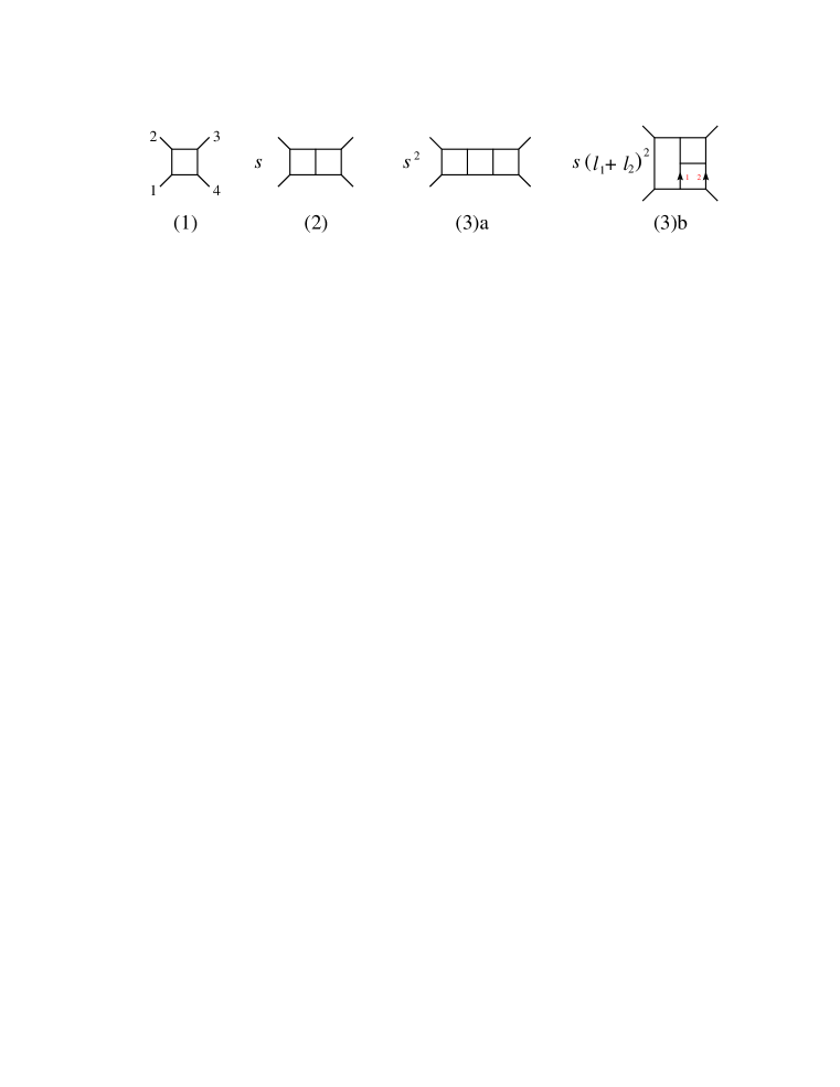
Figure 1: Integrals required for $gg\to gg$ scattering in planar MSYM at one loop (1), two loops (2) and three loops ((3)a and (3)b). The box (1), planar double box (2) and three-loop ladder (3)a integrals are scalar integrals, with no loop-momentum dependent factors in the numerator. The tennis-court integral (3)b contains a factor of $(l_{1}+l_{2})^{2}$, where $l_{1}$ and $l_{2}$ are marked with arrows in the figure.

The result for the one-loop four-point amplitude is GSB

$$M_{4}^{{(1)}}(\epsilon)=-{1\over 2}\,{\cal I}^{(1)}(s,t)\,,$$ (33)

where the Mandelstam variables are $s=(k_{1}+k_{2})^{2}$ and $t=(k_{2}+k_{3})^{2}$. The factor of $1/2$ in eq. (33) follows from our normalization convention for $A_{n}^{(L)}$, which is defined by eq. (8). The one-loop scalar box integral ${\cal I}_{4}^{(1)}(s,t)$ (multiplied by a convenient normalization factor), depicted in fig. 1, is

$${\cal I}^{(1)}(s,t)\equiv st\,I_{4}^{(1)}(s,t)\,,$$ (34)

where $I_{4}^{(1)}(s,t)$ is defined in eq. (B1) of ref. Iterate3 . We absorb the factor of $st$ into the definition of the integrals we use, because it cancels a factor of $1/(st)$ appearing in the explicit expression for $I_{4}^{(1)}(s,t)$, and matches the form in which it appears in the MSYM amplitudes. This integral is given in terms of HPLs in eq. (B1) of that reference, through the order we require here, ${\cal O}(\epsilon^{4})$. The higher-order terms in $\epsilon$ are needed to be able to evaluate terms in the infrared/iterative representation (32) of the four-loop amplitude through ${\cal O}(\epsilon^{-2})$. For example, in the term $[M_{4}^{(1)}(\epsilon)]^{4}\ \propto\ [{\cal I}^{(1)}(\epsilon)]^{4}$ in eq. (32), if one takes the leading $1/\epsilon^{2}$ term from three of the four factors, then the coefficient of $\epsilon^{4}$ in the fourth factor contributes to the ${\cal O}(\epsilon^{-2})$ term in the product.

The planar two-loop MSYM four-point amplitude is given by BRY

$$M^{(2)}_{4}(\epsilon)={1\over 4}\,\Bigl{[}{\cal I}^{(2)}(s,t)+{\cal I}^{(2)}(t,s)\Bigr{]}\,.$$ (35)

The two-loop scalar double-box integral, shown in fig. 1, is

$${\cal I}^{(2)}(s,t)\equiv s^{2}t\,I_{4}^{(2)}(s,t)\,,$$ (36)

where $I_{4}^{(2)}(s,t)$ is defined in eq. (B4) of ref. Iterate3 . As at one loop, we have rescaled the integral to remove the rational prefactor. This integral was first evaluated through ${\cal O}(\epsilon^{0})$ in terms of polylogarithms SmirnovDoubleBox . Because the infrared/iterative expression (32) contains, for example, $[M_{4}^{(2)}(\epsilon)]^{2}\ \propto\ [{\cal I}^{(2)}(\epsilon)]^{2}$, and because the expansion of ${\cal I}^{(2)}(\epsilon)$ begins at order $1/\epsilon^{4}$, we need its expansion through ${\cal O}(\epsilon^{2})$. This expansion is presented in terms of HPLs in eq. (B5) of ref. Iterate3 .

The three-loop planar amplitude is given by BRY ; Iterate3

$$M^{(3)}_{4}(\epsilon)=-{1\over 8}\,\Bigl{[}{\cal I}^{{(3)}{\rm a}}(s,t)+2\,{\cal I}^{{(3)}{\rm b}}(t,s)+{\cal I}^{{(3)}{\rm a}}(t,s)+2\,{\cal I}^{{(3)}{\rm b}}(s,t)\Bigr{]}\,.$$ (37)

The scalar triple-ladder and non-scalar “tennis-court” integrals, illustrated in fig. 1, are

$${\cal I}^{{(3)}{\rm a}}\equiv s^{3}t\,I_{4}^{{(3)}\rm a}(s,t)\,,$$

$${\cal I}^{{(3)}{\rm b}}\equiv st^{2}\,I_{4}^{{(3)}\rm b}(s,t)\,,$$ (38)

where $I_{4}^{{(3)}\rm a}(s,t)$ and $I_{4}^{{(3)}\rm b}(s,t)$ are defined in eqs. (3.1) and (3.2), respectively, of ref. Iterate3 . Because these integrals multiply ${\cal I}^{(1)}$ in the term $M_{4}^{(1)}(\epsilon)M_{4}^{(3)}(\epsilon)$ in eq. (32), we need their expansion through ${\cal O}(\epsilon^{0})$. These expansions were first carried out in terms of HPLs for $I_{4}^{{(3)}\rm a}$ in ref. SmirnovTripleBox , and for $I_{4}^{{(3)}\rm b}$ in ref. Iterate3 . The results are collected in eqs. (B7) and (B9) of ref. Iterate3 .

The coefficients of the integrals in the two- and three-loop expressions (35) and (37) were originally determined BRY using iterated two-particle cuts. Such cuts can be evaluated to all orders in $\epsilon$ because ${\cal N}=4$ supersymmetry relates all nonvanishing four-point amplitudes; therefore precisely the same algebra enters as at one loop, for which it leads to the amplitude (33). More generally, an ansatz for the planar contributions to the integrands was proposed in terms of a “rung insertion rule” BRY ; BDDPR to be described below, which was based largely on the structure of the iterated two-particle cuts. At three loops, the planar integrals generated by the rung rule can all be constructed using iterated two-particle cuts. Also, the three-loop planar amplitude (37) has the correct infrared poles and a remarkable iterative structure Iterate3 , so there is little doubt that it is the complete answer.

However, beyond three loops — and even at three loops for non-planar contributions — the rung rule generates graphs that cannot be obtained using iterated two-particle cuts. It is less certain that the rung rule gives the correct results for such contributions. Indeed, we shall see that there are additional, non-rung-rule, contributions to the planar amplitude beginning at four loops.

Nevertheless, we start constructing the planar four-loop MSYM amplitude using the diagrams generated by the rung rule. According to this rule, each diagram in the planar $L$-loop amplitude can be used to generate planar $(L+1)$-loop diagrams as follows: First, one generates a set of diagrams by inserting a new line joining each possible pair of internal lines. Next, one removes from this set all diagrams with triangle or bubble subdiagrams. Besides the scalar propagator associated with the new line, one also includes an additional numerator factor for the diagram, beyond that inherited from the $L$-loop diagram, of $i(l_{1}+l_{2})^{2}$. Here $l_{1}$ and $l_{2}$ are the momenta flowing through each of the legs to which the new line is joined. Each distinct $(L+1)$-loop contribution is counted once, even if it can be generated in multiple ways. (Contributions corresponding to identical graphs but with different numerator factors should be counted as distinct.) Rung-rule diagrams have also been referred to as “Mondrian diagrams” because of their visual similarity Iterate3 .

At one loop, the only no-triangle graph for the four-point process is the box graph depicted in fig. 1. In going to two loops, there is only one inequivalent way to add a rung to the box graph without creating a triangle. Connecting opposing sides of the box, we form the planar double box in fig. 1. (One might also imagine attaching a propagator between two adjacent external legs. However, this operation yields the same double box.) To generate the three-loop graphs, we add a rung, either vertically or horizontally, to one of the boxes of the two-loop box diagram, thus yielding the triple ladder (3)a and tennis-court integral (3)b of fig. 1. (Attaching a propagator between external legs again gives nothing new.) Of course, there are several permutations of external legs present for any given type of graph; all of them are produced by the rung rule. Here we are identifying only the topologically distinct integrals that arise.

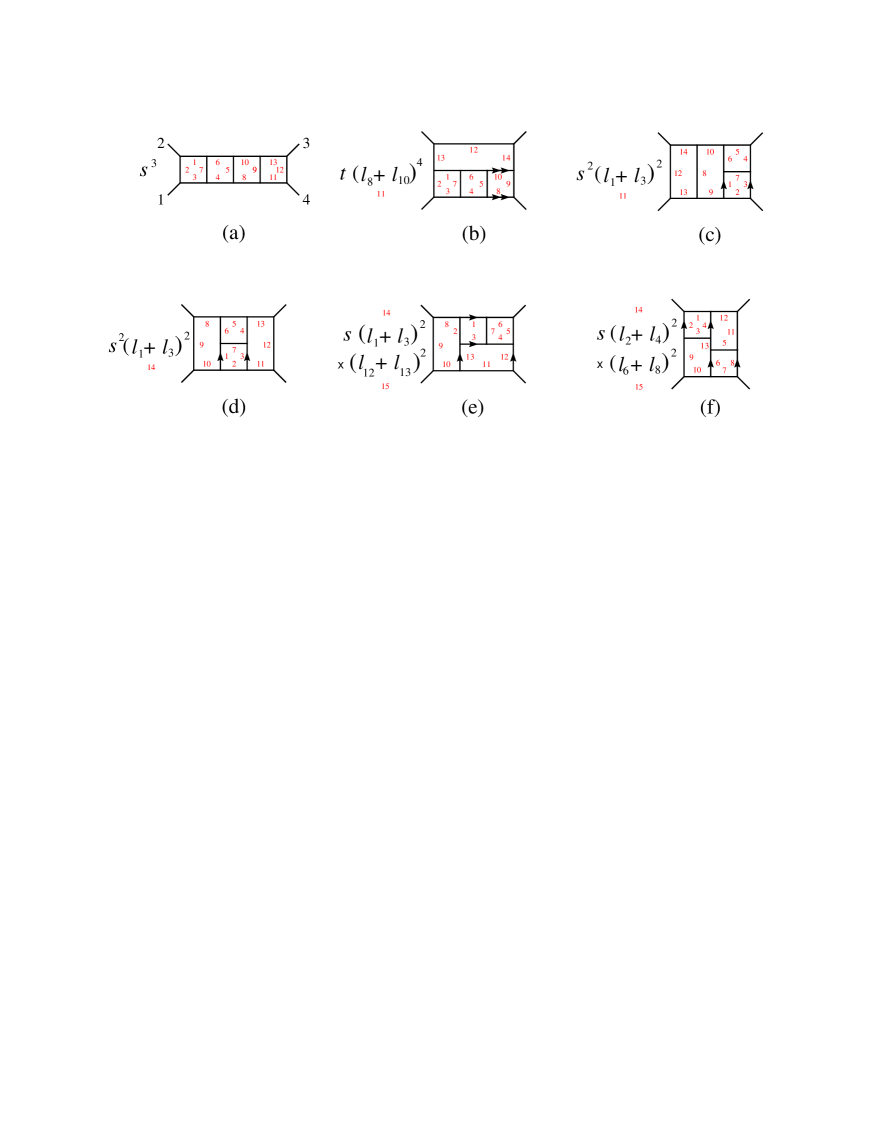
Figure 2: “Rung-rule” contributions to the leading-color four-loop amplitude, in terms of integral functions given in eqs. (129)–(134). An overall factor of $st$ has been suppressed in each figure, compared with the definitions in eqs. (129)–(134).

What happens when we try to add rungs to the three-loop integrals? There are two inequivalent ways to add a rung inside either the left- or the right-most box of the triple ladder integral in fig. 1; these give the integrals of fig. 2(a) and (c). Adding a vertical rung inside the middle box does not yield a topologically distinct integral. Adding a horizontal rung inside the middle box yields the integral of fig. 2(d). Inserting a vertical rung inside the upper-right box of the tennis-court integral in fig. 1 gives us fig. 2(e), and a horizontal one, fig. 2(b). Finally, adding a horizontal rung inside the left-side box of the tennis-court integral gives us a new kind of integral, shown in fig. 2(f), which has no two-particle cuts.

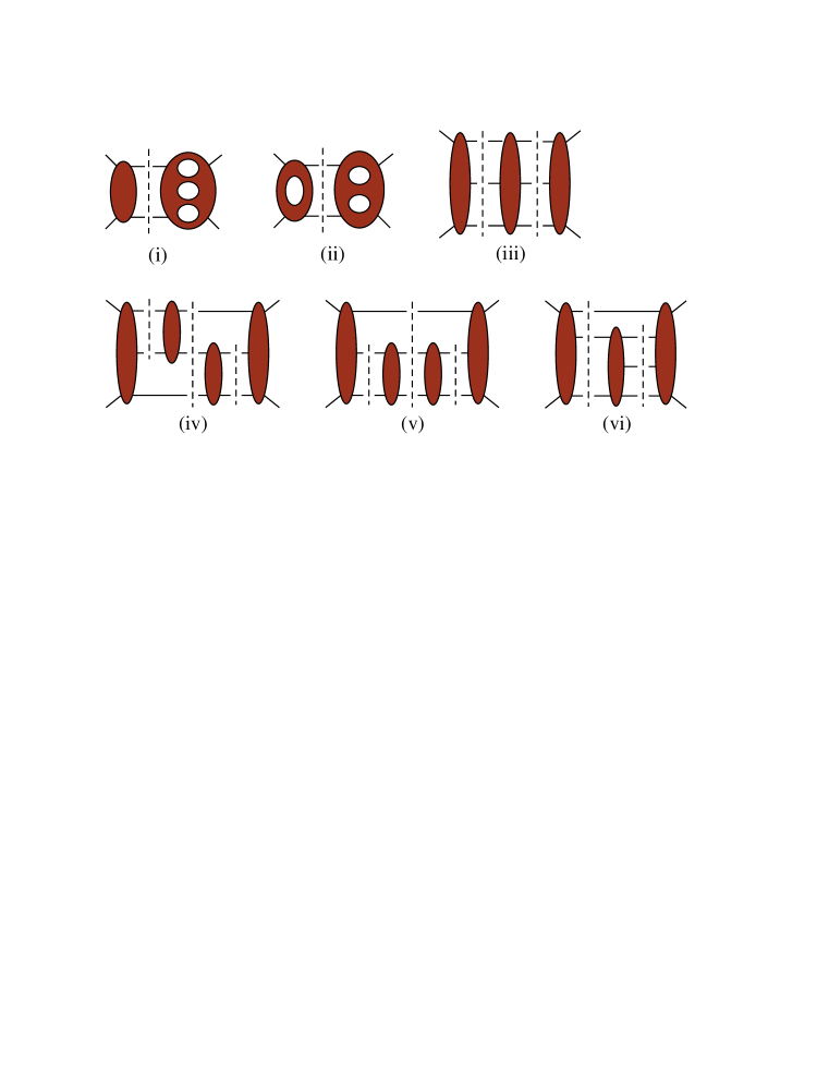
Figure 3: Generalized cuts that provide information about the planar four-loop amplitude. (i) A two-particle cut separating a tree amplitude from a three-loop amplitude. (ii) A two-particle cut separating a one-loop amplitude from a two-loop amplitude. (iii) A “3–3” cut separating the amplitude into a product of three tree amplitudes. (iv) An “upper-2–3–lower-2” cut separating the amplitude into a product of four tree amplitudes. (v) A “lower-2–3–lower-2” cut. (vi) A “3–lower-3” cut.

The propagators and momentum numerators present in integrals fig. 2(a)–(e) are determined by the two-particle cuts, as depicted in fig. 3(i) and (ii). That is, the rung rule is guaranteed to be correct for them. There is no such guarantee for integral fig. 2(f), which has no two-particle cut with real external momenta. In order to check it, we need to compute a three-particle cut. We chose to perform the generalized-unitarity cut of fig. 3(iv), a threefold-cut with a central three-particle cut and two secondary two-particle cuts. This cut reveals that the rung rule is more robust than might have been expected, based on its origin in iterated two-particle cuts: The rule does in fact give the correct form for the numerator of the integral in fig. 2(f), even though no two-particle cut can detect it.

Because we have no proof that the $(-2\epsilon)$-dimensional parts of loop momenta are unimportant to the computation, we perform these calculations in $D$ dimensions. For this purpose, we need tree amplitudes with (some of) the external states kept in general dimension. In the three-particle cuts, one has contributions from three-gluon states, and from states with gluons and fermion (gluino) pairs crossing the cut, in addition to states with scalar pairs or fermion pairs and a lone scalar. In principle, one could evaluate these cuts by computing all the required amplitudes, and summing over the particle multiplet. However, it is easier to use a trick. The trick takes advantage of the fact that the MSYM multiplet, consisting of the gluon, four Majorana fermions, and six real scalars, can also be understood as a single ${\cal N}=1$ multiplet in ten dimensions. Instead of summing over the multiplet seen as the ${\cal N}=4$ multiplet in four dimensions, we sum over the ${\cal N}=1$ multiplet in ten dimensions. This trick reduces the number of types of intermediate states one has to consider, though of course the total number of states is unchanged. The loop momenta are in any event kept in $D$ dimensions. (The trick is compatible with the FDH regularization scheme FDH , where the momenta are taken to be in $D$ dimensions, but the number of states in the loops is kept at the four-dimensional value.)

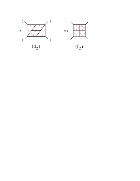
Figure 4: Non-rung-rule contributions to the leading-color four-loop amplitude, in terms of integral functions defined in eqs. (135) and (136). Integral (d₂) follows the labeling of integral (d) in fig. 2, and integral (f₂) follows the labeling of integral (f). An overall factor of $st$ has been suppressed in each figure, compared with eqs. (135) and (136).

The cut of fig. 3(iv) also reveals the presence of a non-rung-rule integral, shown in fig. 4(d₂). The integral has, of course, no two-particle cuts, but it can be obtained from the integral topology of fig. 2(d) by canceling two propagators, labeled 10 and 13. The integral of fig. 2(f) could also have been checked using another generalized-unitarity cut, the two-fold three-particle cut of fig. 3(iii). This cut also reveals the presence of the “four-square” integral, shown in fig. 4(f₂). This integral can be obtained from the topology of fig. 2(f) by canceling the propagator labeled 13. The cut of fig. 3(iii) also detects the integral of fig. 4(d₂).

Under mild assumptions, which we discuss in section V, it is sufficient to compute two additional multiple cuts, shown in fig. 3(v) and (vi), in order to rule out any additional contributions. We have computed these cuts, and we indeed find that no additional integrals appear.

IV Integral representation of the four-loop planar amplitude

We find that the four-loop planar amplitude is given by

$$M^{(4)}_{4}(\epsilon) = {1\over 16}\Bigl{[}{\cal I}^{\rm(a)}(s,t)+{\cal I}^{\rm(a)}(t,s)+2\,{\cal I}^{\rm(b)}(s,t)+2\,{\cal I}^{\rm(b)}(t,s)+2\,{\cal I}^{\rm(c)}(s,t)+2\,{\cal I}^{\rm(c)}(t,s)$$ (39)

$$\hskip 11.38092pt\hbox{}+{\cal I}_{4}^{\rm(d)}(s,t)+{\cal I}^{\rm(d)}(t,s)+4\,{\cal I}^{\rm(e)}(s,t)+4\,{\cal I}^{\rm(e)}(t,s)+2\,{\cal I}^{\rm(f)}(s,t)+2\,{\cal I}^{\rm(f)}(t,s)$$

$$\hskip 11.38092pt\hbox{}-2\,{\cal I}^{\rm(d_{2})}(s,t)-2\,{\cal I}^{\rm(d_{2})}(t,s)-{\cal I}^{\rm(f_{2})}(s,t)\Bigr{]}\,.$$

The rung-rule integrals ${\cal I}^{\rm(a)}$ through ${\cal I}^{\rm(f)}$ are depicted in fig. 2. The two additional integrals, ${\cal I}^{\rm(d_{2})}$ and ${\cal I}^{\rm(f_{2})}$, depicted in fig. 4, do not follow from the rung rule, and were detected using generalized cuts with at least one three-particle channel, as discussed in section III.

The integrals appearing in the four-point amplitude are defined generically, for diagram “$(x)$” by

$${\cal I}^{(x)}(s,t)\equiv(-ie^{\epsilon\gamma}\pi^{-d/2})^{4}\int\mbox{d}^{d}p\,\mbox{d}^{d}q\,\mbox{d}^{d}u\,\mbox{d}^{d}v\ {st\,{\cal N}^{(x)}\over\prod_{j}p_{j}^{2}}\,,$$ (40)

where $p,q,u,v$ are the four independent loop integration variables, and $d=4-2\epsilon$. The product in the denominator of eq. (40) runs over the labels of internal lines in the graph $(x)$. (For graphs (b) and (c), line 11 corresponds to a numerator factor, so it should be excluded from this product. Similarly, lines 10 and 13 are to be omitted from the denominator product for graph (d₂), and line 13 from the product for graph (f₂).) Each line carries momentum $p_{j}$, which is some linear function of $p,q,u,v$ and the external momenta. The line label $j$ is shown next to each internal line. The numerator factor ${\cal N}^{(x)}$ is also shown explicitly, to the left of the graph for $(x)$. We have omitted an overall factor of $st$ from ${\cal N}^{(x)}$ associated with each integral from the figure, in order to avoid cluttering it.

For the quadruple-ladder graph (a), and for the non-rung-rule graphs (d₂) and (f₂), ${\cal N}^{(x)}$ is completely independent of the loop momentum, and so it may be pulled outside of the integral. For the other graphs, at least one factor in ${\cal N}^{(x)}$ depends on the loop momenta. In generating a Mellin-Barnes representation for these integrals, we think of these factors as additional “propagators” appearing in the numerator instead of the denominator. Accordingly, we attach a line label $j$ to each such factor. The presence of such a factor is also indicated graphically by a pair of parallel arrows, marking the lines whose momenta are summed, then squared, to generate the numerator factor.

For example, the quadruple ladder integral (a) is defined by

$${\cal I}^{\rm(a)} = (-ie^{\epsilon\gamma}\pi^{-d/2})^{4}\,s^{4}t\int{\mbox{d}^{d}p\,\mbox{d}^{d}r\,\mbox{d}^{d}u\,\mbox{d}^{d}v\over p^{2}\,(p-k_{1})^{2}\,(p-k_{1}-k_{2})^{2}\,q^{2}\,(p-q)^{2}\,(q-k_{1}-k_{2})^{2}}$$ (41)

$$\hskip 85.35826pt\times{1\over u^{2}\,(q-u)^{2}\,(u-k_{1}-k_{2})^{2}\,v^{2}\,(u-v)^{2}\,(v-k_{1}-k_{2})^{2}\,(v+k_{4})^{2}}$$

$$= (-ie^{\epsilon\gamma}\pi^{-d/2})^{4}\int{\mbox{d}^{d}p\,\mbox{d}^{d}r\,\mbox{d}^{d}u\,\mbox{d}^{d}v\ s^{4}t\over\prod_{j=1}^{13}p_{j}^{2}}\,.$$

Similarly, integral (b) is defined by

$${\cal I}^{\rm(b)} = (-ie^{\epsilon\gamma}\pi^{-d/2})^{4}\,st^{2}\int{\mbox{d}^{d}p\,\mbox{d}^{d}r\,\mbox{d}^{d}u\,\mbox{d}^{d}v\ [(v+k_{1})^{2}]^{2}\over p^{2}\,(p-k_{1})^{2}\,(p-v-k_{1})^{2}\,\,q^{2}\,(p-q)^{2}\,(q-v-k_{1})^{2}}$$ (42)

$$\hskip 85.35826pt\times{1\over u^{2}\,(q-u)^{2}\,(u-v-k_{1})^{2}\,(u+k_{4})^{2}\,v^{2}\,(v-k_{2})^{2}\,(v-k_{2}-k_{3})^{2}}$$

$$= (-ie^{\epsilon\gamma}\pi^{-d/2})^{4}\int{\mbox{d}^{d}p\,\mbox{d}^{d}r\,\mbox{d}^{d}u\,\mbox{d}^{d}v\ st^{2}\,(p_{11}^{2})^{2}\over p_{12}^{2}\,p_{13}^{2}\,p_{14}^{2}\prod_{j=1}^{10}p_{j}^{2}}\,.$$

The double arrows indicate that in this case the numerator factor appears squared, $(p_{11}^{2})^{2}\equiv(l_{8}+l_{10})^{4}=[(v+k_{1})^{2}]^{2}$.

V Establishing the correctness of the integrand

In this section we justify the result (39) for the four-loop planar amplitude, based upon our evaluation of the unitarity cuts. Because we have not evaluated all possible unitarity cuts, we have to impose some mild assumptions about the types of integrals that should be present. We will see that another, stronger assumption of conformal invariance also holds for the individual integrals that appear, although we do not require it. In addition, as we shall see in the next section, the agreement of the infrared singularities through ${\cal O}(\epsilon^{-2})$ with their known form MagneaSterman — up to the one unknown constant at ${\cal O}(\epsilon^{-2})$ — provides a non-trivial consistency check on our construction.

The analysis determining the integrand of the four-loop four-point amplitude proceeds in several steps:

• We assume that there are no integrals with triangle or bubble subgraphs.

• We classify the four-loop planar integrals of this type topologically. We begin with the subset of graphs having only cubic vertices, from which we can obtain the remaining graphs.

• We construct a set of generalized cuts capable of detecting all such integrals. That is, each such integral, when restricted to the generalized cut kinematics, should be nonvanishing for at least one cut in the set. For it to be nonvanishing, it must have a propagator present for each line being cut. We used this set of cuts to deduce the terms in the expression (39). Indeed, we find that each such cut of the expression is completely consistent with our evaluation of the cut. This step confirms the result, under the “no triangle” assumption.

• Alternatively, we consider the result of assuming that only conformally-invariant integrals contribute, when the external legs are taken off-shell so that the integrals become well-defined (finite) in four dimensions. Such integrals were considered recently in ref. DHSS . We find that the conformal-invariance assumption is a powerful one; it allows all eight integrals contributing to eq. (39) to be present, while forbidding all but two of the additional no-triangle integrals. The potential contributions of these remaining two integrals are easily ruled out by examining the two-particle cuts.

Next we elaborate on each step in the analysis.

V.1 Unitarity construction

Our assumption, that there are no integrals with triangle or bubble subgraphs in multi-loop ${\cal N}=4$ super-Yang-Mills theory, is sometimes referred to as the “no triangle hypothesis”. (Such an assumption also appears to be applicable to ${\cal N}=8$ supergravity, at least at one loop GravNoTriangle .) We now discuss evidence in favor of this hypothesis. First, notice that a bubble subgraph would lead to an ultraviolet subdivergence. In the absence of cancellations between different integral topologies, such subdivergences are forbidden by the finiteness of MSYM Finiteness . Keep in mind that all cancellations between different particles in the supermultiplet have already been taken into account, so the coefficients of all bubble integrals should indeed be zero.

Next, suppose there were a triangle subgraph in some multi-loop integral. Excise a region around the triangle, cutting through open propagators attached to the integral. This excised region represents a one-particle-irreducible triangle-type contribution to a one-loop $n$-particle scattering amplitude. If all $n$ cut legs are gluons, then we know that such a contribution is forbidden in MSYM, for arbitrary $n$, by applying loop-momentum power-counting to a computation of the one-loop amplitude using background-field gauge SuperspaceBook ; NeqFourOneLoop . However, in the present case some of the $n$ legs might be associated with other fields of the ${\cal N}=4$ supermultiplet. Supersymmetry Ward identities SWI typically relate many such amplitudes to the gluonic case, but we do not know of a general proof. Thus we do not claim to have a full proof that all topologies with triangle subgraphs are absent, although we strongly suspect that it is the case.

We now wish to classify the four-loop planar integrals containing no triangle or bubble subgraphs. We can perform this classification first for the subset of such graphs that have only cubic (three-point) vertices, for the following reason: If a graph contains a quartic or higher-point vertex, we can “resolve” the vertex into multiple three-point vertices by moving some of the lines attached to the vertex. Such a procedure never decreases the number of propagators associated with a given loop. Therefore a no-triangle graph will remain a no-triangle graph under this procedure. So, if we know all the no-triangle graphs with only cubic vertices, we can get every remaining no-triangle graph by sliding cubic vertices together until they coincide, a procedure known as “canceling propagators”.

Figure 5: The only one-particle-irreducible purely-cubic four-loop four-point graph with no triangle or bubble subgraphs, besides the rung-rule graphs in fig. 2.

The cubic subset can be classified iteratively in the number of loops using the Dyson-Schwinger equation. In order to use the Dyson-Schwinger approach for the case at hand, the planar four-loop four-point amplitude, we also need to classify the planar cubic no-triangle graphs of the following types: one loop for the number of legs $n$ up to 7, two loops for $n$ up to 6, and three loops for $n$ up to 5. The result is that there are a total of 13 planar cubic four-loop four-point no-triangle graphs. Of the 13 graphs, seven are one-particle-irreducible. Six of these seven have the topology of the rung-rule graphs shown in fig. 2. The seventh is shown in fig. 5. Note that here we are only classifying graphs, and not yet specifying the loop-momentum polynomials associated with each graph.

The six one-particle-reducible graphs can be obtained by sewing external trees onto four-loop graphs with either two or three external legs. (There are no planar cubic no-triangle graphs at four loops with fewer than two external legs.) From the point of view of the cuts, these one-particle-reducible graphs are equivalent to certain of the non-cubic graphs obtained by canceling external propagators, so we shall defer their description briefly.

Figure 6: No-triangle planar four-loop graphs, in addition to those given in figs. 2 and 4. The notation indicates the rung-rule graph in fig. 2, or graph (g) in fig. 5, that a given graph here is derived from by canceling propagators.

The next step is to cancel propagators between vertices in the cubic graphs in figs. 2 and 5. That is, we merge adjacent three-point vertices into four-point (or higher-point) vertices by eliminating the line(s) between them, while insisting on at least four propagators around every sub-loop. This procedure is also straightforward to carry out. It generates the two non-rung-rule graphs in the expression (39), shown in fig. 4, as well as the 16 additional graphs shown in fig. 6. We have given each graph a notation which indicates the rung-rule graph (or graph (g)) from which it can be generated by canceling one or more propagators. For example, graph (b₃) is found by canceling propagators 13 and 14 in rung-rule graph (b), and graph (e₆) is found by canceling propagators 8 and 11 in rung-rule graph (e).

Some graphs in fig. 6 can be generated from more than one cubic graph. In fact, five of the six one-particle-reducible cubic graphs mentioned earlier are equivalent, upon canceling external propagators, to diagrams in fig. 6, namely graphs (b₂), (d₃), (d₅), (e₁), and (g₁). Hence we do not provide a separate figure for the one-particle-reducible cubic graphs. The sixth graph has the form of a massless version of graph (d₅), sewn as an external bubble to a four-point tree graph. Such integrals vanish in dimensional regularization, so we need not consider them.

To complete the direct justification of the four-loop result (39), given the no-triangle assumption, we just need to show that each graph appearing in figs. 2, 4, 5 and 6 can be detected by at least one of the generalized cuts we have computed, out of the six cuts shown in fig. 3. Table 1 summarizes some of the cuts that detect the no-triangle graphs. For some of the graphs, other cuts also detect them, but for brevity they were not listed in the table. Almost all graphs appear in multiple cuts. Only two of the graphs, (b₄) and (e₆), appear in a unique cut, the “3–lower-3” cut labeled (vi) in fig. 3.

Table 1: The no-triangle graphs, and some of the cuts from fig. 3 that detect them. (In some cases, the diagram must be rotated or flipped first.)

Graph	Cuts	Graph	Cuts	Graph	Cuts
(a)	(i), (ii), (iii)	(b1)	(v), (vi)	(d5)	(i), (iii), (iv)
(b)	(i), (v)	(b2)	(i), (vi)	(e1)	(i), (iii), (iv)
(c)	(i), (ii), (iii), (iv)	(b3)	(v), (vi)	(e2)	(iii), (iv)
(d)	(i), (iii), (v)	(b4)	(vi)	(e3)	(i), (vi)
(e)	(i), (iii), (iv), (vi)	(c1)	(i), (iii), (iv)	(e4)	(i), (vi)
(f)	(iii), (iv), (vi)	(d1)	(i), (iii), (iv)	(e5)	(i), (iii), (iv)
(d2)	(iii), (iv)	(d3)	(i), (iii), (iv)	(e6)	(vi)
(f2)	(iii), (vi)	(d4)	(i), (iii), (iv)	(g)	(i), (vi)
				(g1)	(i), (vi)

V.2 Conformal properties

We have finished our justification of the representation (39) for the four-loop planar amplitude. In the rest of this section we would like to examine the consequences of making a stronger assumption than the no-triangle hypothesis. This assumption is that each of the integral functions that appears is conformally invariant. Here we are inspired by the discussion of conformally-invariant integrals by Drummond, Henn, Sokatchev, and one of the authors DHSS . Although the requirement of conformal invariance is natural because of the conformal invariance of the theory in four dimensions, we do not have a proof that these integrals are the only ones that can appear in the amplitudes. Nevertheless, as we shall see, the conformal properties offer a rather useful guide. (It is possible that extensions of the conformal-invariance analysis in ref. GKS could be used to prove that only such conformally invariant integrals can be present.)

We actually wish to study the conformal properties of the integrals in four dimensions, yet they are ill-defined there because of the infrared divergences associated with on-shell, massless external legs. We therefore adopt a different infrared regularization of the integrals by taking the external legs off shell, letting $k_{i}^{2}\neq 0$, $i=1,2,3,4$, instead of using a dimensional regulator as in the rest of the paper. We demand that each integral that appears be conformally invariant. Actually, the integrals need only transform covariantly, carrying conformal weights associated with each of the external legs, in such a way that they can be made invariant by multiplying by appropriate overall factors of $s$ or $t$. In canceling the conformal weights using the external invariants, we should not use any factors that vanish as the external legs return on shell, in the limit $k_{i}^{2}\to 0$. Such factors would lead to power-law divergences or to vanishings of the integrals that are too severe, compared to the typical logarithmic dependences on $k_{i}^{2}$ from the known form of infrared singularities. Thus integrals that require powers of $k_{i}^{2}$ to be conformally invariant should not appear in any on-shell amplitude. This on-shell restriction turns out to be a powerful one.

The net result of the conformal-invariance requirement will be that, besides the eight integrals already present in eq. (39) and figs. 2 and 4, remarkably only two other potential conformal integrals survive. The first of them is the (d₅) graph from fig. 6. This graph has the structure of a potential propagator correction at four loops. However, in the context of the $gg\to gg$ scattering amplitude of the ${\cal N}=4$ theory, it can be excluded very simply, without computing any generalized cuts. One only has to use the structure of the three-loop amplitude, and the simplest two-particle cut, cut (i) in fig. 3, to see that it cannot be present. The second of the additional potential integrals has the topology of integral (d) in fig. 2, but it has a different numerator factor, to be described below. This new integral, (d^′), is also easy to exclude using the same two-particle cut (i) in fig. 3.

It is rather striking that every integral identified via the unitarity cuts is conformally invariant, and that there are only two other conformal integrals, which can be eliminated easily via two-particle cuts. Furthermore, the two integrals that are not present differ from the eight that are present in how the conformal invariance is achieved, as we shall discuss below.

To analyze the conformal invariance properties, we shall use changes of variables as suggested in ref. DHSS . (The same conformal integrals appear in coordinate-space correlators of gauge invariant operators Schubert ; the coincidence is presumably an accident of there being a limited number of conformal integrals.) As an example, consider the two-loop double box depicted in fig. 1,

$${\cal I}^{(2)}(s,t) = (-ie^{\epsilon\gamma}\pi^{-2})^{2}s^{2}t$$ (43)

$$\hskip 8.53581pt\times\int{{\rm d}^{4}p\ {\rm d}^{4}q\over p^{2}(p-k_{1})^{2}(p-k_{1}-k_{2})^{2}q^{2}(q-k_{4})^{2}(q-k_{3}-k_{4})^{2}(p+q)^{2}}\,.\hskip 22.76219pt$$

We have taken $d=4$, with the $k_{i}$ off shell to serve as an infrared regulator. Next, use the change of variables,

$$k_{1}=x_{41}\,,\hskip 22.76228ptk_{2}=x_{12}\,,\hskip 22.76228ptk_{3}=x_{23}\,,\hskip 22.76228ptk_{4}=x_{34}\,,\hskip 22.76228ptp=x_{45},\hskip 22.76228ptq=x_{64}\,,$$ (44)

where $x_{ij}\equiv x_{i}-x_{j}$. This choice of variables automatically ensures that momentum is conserved, $k_{1}+k_{2}+k_{3}+k_{4}=0$. Note that the external invariants become

$$s=(k_{1}+k_{2})^{2}=x_{24}^{2}\,,\hskip 28.45274ptt=(k_{2}+k_{3})^{2}=x_{13}^{2}\,.$$ (45)

Performing the change of variables (44) in the double box, we obtain,

$${\cal I}^{(2)}(x_{1},x_{2},x_{3},x_{4})=(-ie^{\epsilon\gamma}\pi^{-2})^{2}x_{24}^{4}x_{13}^{2}\int{\rm d}^{4}x_{5}\ {\rm d}^{4}x_{6}\,{1\over x_{45}^{2}x_{15}^{2}x_{25}^{2}x_{46}^{2}x_{36}^{2}x_{62}^{2}x_{56}^{2}}\,.$$ (46)

The principal conformal-invariance constraints on integrals constructed from the invariants $x_{ij}^{2}$ are exposed by performing an inversion on all points, $x_{i}^{\mu}\rightarrow{x_{i}^{\mu}/x_{i}^{2}}$. (We cannot impose such an inversion on the $k_{i}$ directly, because it would violate the constraint of momentum conservation.) Under the inversion, we have

$$x_{ij}^{2}\rightarrow{x_{ij}^{2}\over x_{i}^{2}x_{j}^{2}}\,,\hskip 28.45274pt{{\rm d}^{4}x_{5}}\rightarrow{{\rm d}^{4}x_{5}\over x_{5}^{8}}\,,\hskip 28.45274pt{{\rm d}^{4}x_{6}}\rightarrow{{\rm d}^{4}x_{6}\over x_{6}^{8}}\,.$$ (47)

It is easy to see that the planar double-box integral is invariant under inversion, i.e. ${\cal I}^{(2)}(x_{1},x_{2},x_{3},x_{4})\ \rightarrow\ {\cal I}^{(2)}(x_{1},x_{2},x_{3},x_{4}).$ For this result to hold, it is important that the unintegrated points $x_{1},x_{2},x_{3},x_{4}$ appear in the numerator just enough times to cancel their appearance in the denominator. The integrated points $x_{5},x_{6}$ each appear four times in the denominator. The dimensionally-regulated version of the conformally-invariant integral ${\cal I}^{(2)}(x_{1},x_{2},x_{3},x_{4})$ is precisely the form in which the two-loop double box appears in the two-loop planar amplitude (35).

In order to analyze the conformal properties of integrals beyond two loops, it is helpful to follow the discussion of ref. DHSS , and introduce a set of dual diagrams Nakanishi . We construct the dual to a diagrammatic representation of a planar loop-momentum integral by placing vertices corresponding to the $x_{i}$ at the centers of the loops and in between pairs of external lines. Denominator factors of $x_{ij}^{2}$ are denoted by drawing dark solid (blue) lines between the corresponding vertices. Numerator factors are denoted by drawing dotted lines between the corresponding vertices. One solid line crosses each propagator in a loop. The conformal weight in each $x_{i}$ variable is then given by the number of solid lines entering the corresponding vertex, less the number of dotted lines. A conformally-invariant integral will have weight four at each internal vertex (to balance the weight of the integration measure), and weight zero at each external vertex. In the diagrams, we shall omit one dotted line connecting external vertices $x_{2}$ and $x_{4}$, and another one connecting $x_{1}$ and $x_{3}$, in order to simplify the presentation. These two omitted lines correspond to the overall factor of $st=x_{24}^{2}x_{13}^{2}$ omitted from the momentum-space diagrams in figs. 2 and 4. Expressions for integrals in terms of the $x_{i}$ variables can be read off quickly from the dual diagrams (and vice versa).

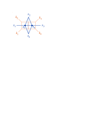
Figure 7: The two-loop planar double box and its dual diagram. The double box is represented by light colored lines and the dual diagram by dark (blue) lines. A dark line connecting $x_{i}$ with $x_{j}$ represents the factor $1/x_{ij}^{2}$. A dotted line signifies a numerator factor of $x_{ij}^{2}$. The momentum corresponding to any $x_{ij}$ is given by the sum of momenta of the light lines crossing the dark line joining $x_{i}$ and $x_{j}$. An overall factor of $st$ has been removed for clarity.

For example, fig. 7 contains the diagram dual to the double box. Each of the solid lines starting at an $x_{i}$ and ending at an $x_{j}$ corresponds to a factor of $1/x_{ij}^{2}$ appearing in eq. (46), while the dotted line corresponds to a factor of $x_{24}^{2}=s$. With this identification the dual figure is in direct correspondence with eq. (46), after removing one overall factor of $st=x_{24}^{2}x_{13}^{2}$ (in order to reduce the visual clutter in the diagram). Because the number of solid lines minus the number of dotted lines at each of the two internal vertices $x_{5}$ and $x_{6}$ is four, the integral is conformally invariant with respect to these points. Similarly, since each of the external points $x_{1},x_{2},x_{3},x_{4}$ has one more solid line than dotted line emanating from it, the conformal weight is unity. If we multiply back by the $x_{24}^{2}x_{13}^{2}$ factor removed previously, then we obtain an integral which is conformally invariant with respect to the external as well as internal points.

The assumption of conformal invariance for the integrals immediately implies the “no-triangle” rule for the momentum-space diagrams. A loop with only three propagators would necessarily result in a negative weight for the $x$ point corresponding to the loop momentum, because only three lines enter the dual diagram vertex. That negative weight can only be eliminated by additional denominator powers of $x$ — that is, by additional propagators which would turn the triangle subgraph into at least a box subgraph.

By placing the dual diagrams on top of the original momentum-space diagrams, we can read off directly the change of variables between the $x_{ij}$ and the momenta: $x_{ij}$ is just the sum of the momenta of the each momentum-space line crossed by the dual line running from $x_{i}$ to $x_{j}$. In the rung-insertion rule, when a rung is inserted between two parallel lines with momenta $l_{1}$ and $l_{2}$, to go from an $L$-loop contribution to an $(L+1)$-loop one, the loops on either side of the parallel lines have acquired a new propagator. Hence each of their dual $x$ vertices has a new solid line emanating from it. The rung-rule momentum-insertion factor of $i(l_{1}+l_{2})^{2}$ is represented by a dotted line stretching between the two vertices, so it restores the conformal invariance for those two loops. This property may help to explain the form of the rung rule.

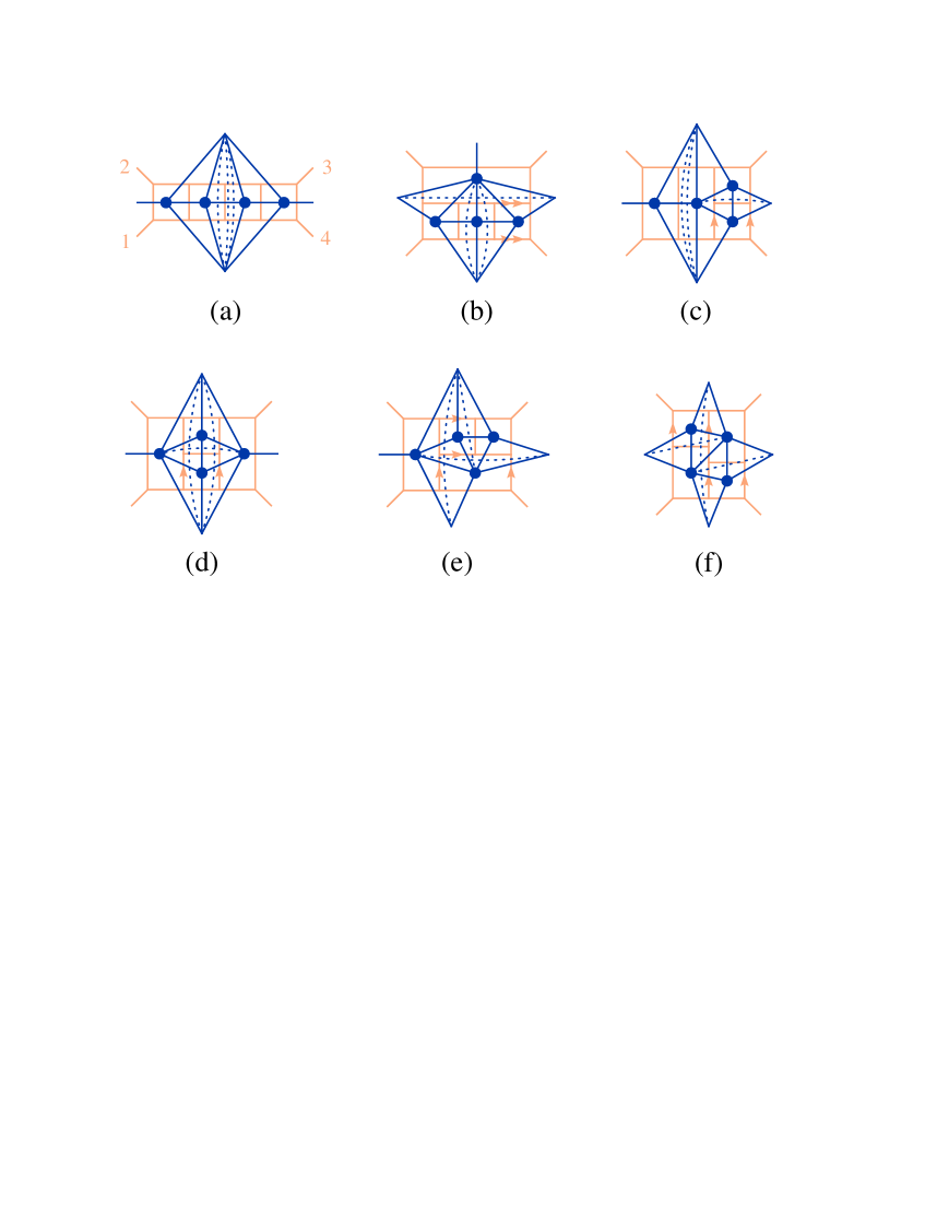
Figure 8: The rung-rule dual diagrams. A factor of $st$ has been removed.

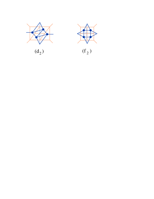
Figure 9: The non-rung rule dual diagrams. A factor of $st$ has been removed.

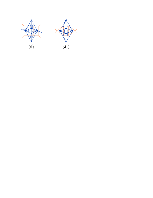
Figure 10: The two four-loop dual integrals, in addition to those given in figs. 2 and 4, that survive the requirement of conformal invariance. Both integrals are ruled out by two-particle cuts. In this case, no factor of $st$ has been removed.

Let us now focus on four-loop four-point integrals. We may find all conformally-invariant integrals by drawing the set of all dual diagrams that have conformal weight zero with respect to all $x_{i}$. Again to prevent cluttering the diagrams in figs. 8 and 9 with dotted lines we have removed a factor of $st$ from the figures. The complete list of conformal four-loop integrals, as it turns out, contains the rung-rule diagrams of fig. 8, the non-rung-rule diagrams of fig. 9, and the two extra integrals shown in fig. 10.

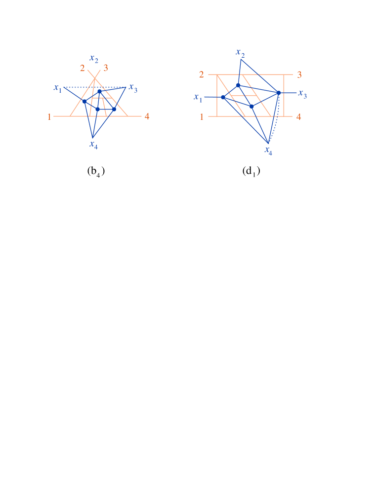
Figure 11: Two examples of dual diagrams which do not lead to new conformal integrals in the on-shell limit, for reasons discussed in the text.

Because conformal invariance in the sense discussed above implies the “no-triangle” rule, the complete list of candidate graphs for conformal integrals are given by the same no-triangle list described above, namely the diagrams in figs. 2, 4, 5 and 6. Upon attempting to draw the dual diagrams to figs. 5 and 6, we find that in all cases except (d₅), either it is impossible to add dotted or even solid lines so as to obtain a conformally-invariant integral, or the obtained conformally-invariant cases are equivalent to previously-included cases, or else conformal invariance can only be achieved by adding solid or dotted lines connecting neighboring external vertices. The latter lines are not admissible, however, because differences of neighboring external $x$ points correspond to individual external momenta $k_{i}$. The corresponding factors are then $k_{i}^{2}$. Their presence would lead to an unwanted power-law vanishing or divergence of the integral in the on-shell limit.

Figure 11 illustrates two examples of dual diagrams that cannot be made conformal, or that reduce to previous cases. First consider the graph labeled (b₄). The internal dual points all have weight four, so no dotted lines can attach to them. The dotted line shown between external points $x_{1}$ and $x_{3}$ reduces the $x_{1}$ weight to zero and the $x_{3}$ weight to one. It is nonvanishing in the massless limit. However, there is no other numerator factor available that is nonvanishing in this limit, to further reduce the conformal weights of external legs $x_{3}$ and $x_{4}$. In particular, $x_{34}^{2}=k_{4}^{2}\to 0$ in the on-shell limit.

As a second example, consider the graph labeled (d₁) in fig. 11. Here there is one pentagon subgraph, and hence one internal $x$ point to which a dotted line can attach. The dotted line shown can be used to reduce the conformal weight of $x_{4}$ from three to two, which would then balance its weight with that of the opposite external point $x_{2}$. (Balanced opposing weights can always be reduced to zero using powers of $s=x_{24}^{2}$ or $t=x_{13}^{2}$.) However, this choice of dotted line merely cancels the propagator that it crosses, and thereby reduces the (d₁) graph to the (d₂) graph in fig. 9, which we already know is conformally invariant and present in the four-loop planar amplitude. Without using the dotted line shown, it is impossible to balance the $x_{4}$ conformal weight, in the massless limit, so the only surviving possibility reduces to an existing integral.

It is curious that the two conformally-invariant integrals represented in fig. 10, which are not present in the planar four-loop four-point amplitude, can be distinguished from the eight in figs. 8 and 9 that are present, by the fact that they do not have explicit overall factors of both $s$ and $t$. As drawn in fig. 10, they have three powers of $s$, but no powers of $t$. The integral (d^′) has the same basic topology as (d) in fig. 9, but the dotted lines emanating from the two pentagon loops are connected to external legs $x_{1}$ and $x_{3}$ instead of to each other. So it has two “rung-rule-type” numerator factors involving the squares of the sums of three loop momenta, but no power of $t$. At the moment, however, we have no good argument why explicit factors of both $s$ and $t$ have to be present in order that an integral be present in the four-point amplitude.

VI Analytic and numerical results

Our next task is to evaluate the integrals entering the four-loop planar amplitude (39) in a Laurent expansion around $\epsilon=0$. For the case at hand, massless gluon-gluon scattering in ${\cal N}=4$ super-Yang-Mills theory, all of the integrals encountered can be evaluated through three loops in terms of a class of functions known as harmonic polylogarithms (HPLs) HPL . We expect this class of functions to continue to suffice at four loops. We know it suffices through ${\cal O}(\epsilon^{-4})$, for which we have analytic results.

VI.1 Analytic expressions through ${\cal O}(\epsilon^{-4})$

The analytic results for the four-loop integrals were obtained with the help of the MB program CzakonMB . We let $x=-t/s$ and $L=\ln(-x)$. Through ${\cal O}(\epsilon^{-4})$ the results, expressed in terms of the HPLs defined in appendix B, are,

$${\cal I}^{\rm(a)}(s,t) = (-t)^{-4\epsilon}\Biggl{\{}{4\over 9\,\epsilon^{8}}+{35\over 72\,\epsilon^{7}}L-{187\,\pi^{2}\over 432\,\epsilon^{6}}$$ (48)

$$\hskip 2.84544pt+\,{10\over 9\,\epsilon^{5}}\Biggl{[}H_{0,0,1}(x)-L\,H_{0,1}(x)+{1\over 2}(L^{2}+\pi^{2})H_{1}(x)+{23\over 48}\pi^{2}L-{1169\over 240}\zeta_{3}\Biggr{]}$$

$$\hskip 2.84544pt+\,{10\over 9\,\epsilon^{4}}\Biggl{[}-22\,H_{0,0,0,1}(x)-H_{0,0,1,1}(x)-H_{0,1,0,1}(x)-H_{1,0,0,1}(x)$$

$$\hskip 36.98866pt+{L}{}(16\,H_{0,0,1}(x)+H_{0,1,1}(x)+H_{1,0,1}(x))-{L^{2}\over 2}(10\,H_{0,1}(x)+H_{1,1}(x))$$

$$\hskip 36.98866pt-{\pi^{2}\over 2}(7\,H_{0,1}(x)+H_{1,1}(x)-L\,H_{1}(x))$$

$$\hskip 36.98866pt+{2\over 3}L^{3}\,H_{1}(x)+\zeta_{3}\,H_{1}(x)-{97\over 12}\zeta_{3}\,L-{2339\over 3600}\pi^{4}\Biggr{]}$$

$$\hskip 2.84544pt+\ {\cal O}(\epsilon^{-3})\Biggr{\}}\,,$$

$${\cal I}^{\rm(b)}(s,t) = (-t)^{-4\epsilon}\Biggl{\{}{4\over 9\,\epsilon^{8}}+{17\over 18\,\epsilon^{7}}L+{1\over\epsilon^{6}}\Biggl{[}{53\over 72}L^{2}-{211\over 432}\pi^{2}\Biggr{]}$$ (49)

$$\hskip 2.84544pt+\,{8\over 9\,\epsilon^{5}}\Biggl{[}H_{0,0,1}(x)-L\,H_{0,1}(x)+{1\over 2}(L^{2}+\pi^{2})H_{1}(x)+{25\over 96}L^{3}-{45\over 64}\pi^{2}L-{601\over 96}\zeta_{3}\Biggr{]}$$

$$\hskip 2.84544pt+\,{8\over 9\,\epsilon^{4}}\Biggl{[}-10\,H_{0,0,0,1}(x)-H_{0,0,1,1}(x)-H_{0,1,0,1}(x)-H_{1,0,0,1}(x)$$

$$\hskip 36.98866pt+L{}\Bigl{(}{71\over 8}\,H_{0,0,1}(x)+H_{0,1,1}(x)+H_{1,0,1}(x)\Bigr{)}-{L^{2}\over 2}\Bigl{(}{31\over 4}\,H_{0,1}(x)+H_{1,1}(x)\Bigr{)}$$

$$\hskip 36.98866pt-{\pi^{2}\over 2}\Bigl{(}3\,H_{0,1}(x)+H_{1,1}(x)-{15\over 8}L\,H_{1}(x)+{73\over 96}L^{2}\Bigr{)}$$

$$\hskip 36.98866pt+{53\over 48}L^{3}\,H_{1}(x)+\zeta_{3}\,H_{1}(x)-{L^{4}\over 48}-{1579\over 96}\zeta_{3}\,L-{743\over 4608}\pi^{4}\Biggr{]}$$

$$\hskip 2.84544pt+\ {\cal O}(\epsilon^{-3})\Biggr{\}}\,,$$

$${\cal I}^{\rm(c)}(s,t) = (-t)^{-4\epsilon}\Biggl{\{}{4\over 9\,\epsilon^{8}}+{13\over 24\,\epsilon^{7}}L+{1\over 18\,\epsilon^{6}}\Biggl{[}L^{2}-{29\over 3}\pi^{2}\Biggr{]}$$ (50)

$$\hskip 2.84544pt+\,{8\over 9\,\epsilon^{5}}\Biggl{[}H_{0,0,1}(x)-L\,H_{0,1}(x)+{1\over 2}(L^{2}+\pi^{2})H_{1}(x)-{L^{3}\over 24}+{\pi^{2}\over 12}L-{1175\over 192}\zeta_{3}\Biggr{]}$$

$$\hskip 2.84544pt+\,{8\over 9\,\epsilon^{4}}\Biggl{[}-{73\over 4}\,H_{0,0,0,1}(x)-H_{0,0,1,1}(x)-H_{0,1,0,1}(x)-H_{1,0,0,1}(x)$$

$$\hskip 36.98866pt+L{}\Bigl{(}{107\over 8}\,H_{0,0,1}(x)+H_{0,1,1}(x)+H_{1,0,1}(x)\Bigr{)}-{L^{2}\over 2}\Bigl{(}{17\over 2}\,H_{0,1}(x)+H_{1,1}(x)\Bigr{)}$$

$$\hskip 36.98866pt-{\pi^{2}\over 2}\Bigl{(}{23\over 4}\,H_{0,1}(x)+H_{1,1}(x)-{7\over 8}L\,H_{1}(x)-{5\over 12}L^{2}\Bigr{)}$$

$$\hskip 36.98866pt+{29\over 48}L^{3}\,H_{1}(x)+\zeta_{3}\,H_{1}(x)+{L^{4}\over 48}-{253\over 32}\zeta_{3}\,L-{5663\over 23040}\pi^{4}\Biggr{]}$$

$$\hskip 2.84544pt+\ {\cal O}(\epsilon^{-3})\Biggr{\}}\,,$$

$${\cal I}^{\rm(d)}(s,t) = (-t)^{-4\epsilon}\Biggl{\{}{4\over 9\,\epsilon^{8}}+{11\over 18\,\epsilon^{7}}L+{1\over 8\,\epsilon^{6}}\Biggl{[}L^{2}-{169\over 54}\pi^{2}\Biggr{]}$$ (51)

$$\hskip 2.84544pt+\,{10\over 9\,\epsilon^{5}}\Biggl{[}H_{0,0,1}(x)-L\,H_{0,1}(x)+{1\over 2}(L^{2}+\pi^{2})H_{1}(x)-{3\over 40}L^{3}-{11\over 80}\pi^{2}\,L-{521\over 240}\zeta_{3}\Biggr{]}$$

$$\hskip 2.84544pt+\,{10\over 9\,\epsilon^{4}}\Biggl{[}-{11\over 5}\,H_{0,0,0,1}(x)-H_{0,0,1,1}(x)-H_{0,1,0,1}(x)-H_{1,0,0,1}(x)$$

$$\hskip 36.98866pt+L{}\Bigl{(}{5\over 2}\,H_{0,0,1}(x)+H_{0,1,1}(x)+H_{1,0,1}(x)\Bigr{)}-{L^{2}\over 2}\Bigl{(}{14\over 5}\,H_{0,1}(x)+H_{1,1}(x)\Bigr{)}$$

$$\hskip 36.98866pt-{\pi^{2}\over 2}\Bigl{(}{2\over 5}\,H_{0,1}(x)+H_{1,1}(x)-{7\over 10}L\,H_{1}(x)-{27\over 40}L^{2}\Bigr{)}$$

$$\hskip 36.98866pt+{31\over 60}L^{3}\,H_{1}(x)+\zeta_{3}\,H_{1}(x)+{3\over 80}L^{4}-{271\over 120}\zeta_{3}\,L-{101\over 600}\pi^{4}\Biggr{]}$$

$$\hskip 2.84544pt+\ {\cal O}(\epsilon^{-3})\Biggr{\}}\,,$$

$${\cal I}^{\rm(e)}(s,t) = (-t)^{-4\epsilon}\Biggl{\{}{4\over 9\,\epsilon^{8}}+{3\over 4\,\epsilon^{7}}L+{1\over\epsilon^{6}}\Biggl{[}{25\over 72}L^{2}-{49\over 108}\pi^{2}\Biggr{]}$$ (52)

$$\hskip 2.84544pt+\,{8\over 9\,\epsilon^{5}}\Biggl{[}H_{0,0,1}(x)-L\,H_{0,1}(x)+{1\over 2}(L^{2}+\pi^{2})H_{1}(x)-{L^{3}\over 24}-{41\over 96}\pi^{2}\,L-{1657\over 384}\zeta_{3}\Biggr{]}$$

$$\hskip 2.84544pt+\,{8\over 9\,\epsilon^{4}}\Biggl{[}-{25\over 4}\,H_{0,0,0,1}(x)-H_{0,0,1,1}(x)-H_{0,1,0,1}(x)-H_{1,0,0,1}(x)$$

$$\hskip 36.98866pt+L{}\Bigl{(}{47\over 8}\,H_{0,0,1}(x)+H_{0,1,1}(x)+H_{1,0,1}(x)\Bigr{)}-{L^{2}\over 2}\Bigl{(}{11\over 2}\,H_{0,1}(x)+H_{1,1}(x)\Bigr{)}$$

$$\hskip 36.98866pt-{\pi^{2}\over 2}\Bigl{(}{7\over 4}\,H_{0,1}(x)+H_{1,1}(x)-{11\over 8}L\,H_{1}(x)-{5\over 12}L^{2}\Bigr{)}$$

$$\hskip 36.98866pt+{41\over 48}L^{3}\,H_{1}(x)+\zeta_{3}\,H_{1}(x)-{13\over 384}L^{4}-{107\over 16}\zeta_{3}\,L-{7153\over 46080}\pi^{4}\Biggr{]}$$

$$\hskip 2.84544pt+\ {\cal O}(\epsilon^{-3})\Biggr{\}}\,,$$

$${\cal I}^{\rm(f)}(s,t) = (-t)^{-4\epsilon}\Biggl{\{}{8\over 9\,\epsilon^{8}}+{107\over 72\,\epsilon^{7}}L+{1\over\epsilon^{6}}\Biggl{[}{49\over 72}L^{2}-{235\over 216}\pi^{2}\Biggr{]}$$ (53)

$$\hskip 2.84544pt+\,{4\over 3\,\epsilon^{5}}\Biggl{[}H_{0,0,1}(x)-L\,H_{0,1}(x)+{1\over 2}(L^{2}+\pi^{2})H_{1}(x)-{7\over 144}L^{3}-{11\over 12}\pi^{2}\,L-{1001\over 144}\zeta_{3}\Biggr{]}$$

$$\hskip 2.84544pt+\,{4\over 3\,\epsilon^{4}}\Biggl{[}-{13\over 2}\,H_{0,0,0,1}(x)-H_{0,0,1,1}(x)-H_{0,1,0,1}(x)-H_{1,0,0,1}(x)$$

$$\hskip 36.98866pt+L{}\Bigl{(}{23\over 4}\,H_{0,0,1}(x)+H_{0,1,1}(x)+H_{1,0,1}(x)\Bigr{)}-{L^{2}\over 2}(5\,H_{0,1}(x)+H_{1,1}(x))$$

$$\hskip 36.98866pt-{\pi^{2}\over 2}\Bigl{(}{11\over 6}\,H_{0,1}(x)+H_{1,1}(x)-{13\over 12}L\,H_{1}(x)-{19\over 48}L^{2}\Bigr{)}$$

$$\hskip 36.98866pt+{17\over 24}L^{3}\,H_{1}(x)+\zeta_{3}\,H_{1}(x)-{5\over 288}L^{4}-{1405\over 144}\zeta_{3}\,L+{4253\over 17280}\pi^{4}\Biggr{]}$$

$$\hskip 2.84544pt+\ {\cal O}(\epsilon^{-3})\Biggr{\}}\,,$$

$${\cal I}^{\rm(d_{2})}(s,t) = (-t)^{-4\epsilon}\Biggl{\{}-{2\over 3\,\epsilon^{5}}\,\zeta_{3}+{1\over\epsilon^{4}}\Biggl{[}-{4\over 3}\,\zeta_{3}\,L+{11\over 432}\,\pi^{4}\Biggr{]}\ +\ {\cal O}(\epsilon^{-3})\Biggr{\}}\,,\hskip 99.58464pt$$ (54)

$${\cal I}^{\rm(f_{2})}(s,t) = (-t)^{-4\epsilon}\Biggl{\{}{16\over 9\,\epsilon^{8}}+{32\over 9\,\epsilon^{7}}L+{1\over\epsilon^{6}}\Biggl{[}{91\over 36}L^{2}-{235\over 108}\pi^{2}\Biggr{]}$$ (55)

$$\hskip-2.84544pt+\,{8\over 3\,\epsilon^{5}}\Biggl{[}H_{0,0,1}(x)-L\,H_{0,1}(x)+{1\over 2}(L^{2}+\pi^{2})H_{1}(x)+{29\over 144}L^{3}-{199\over 144}\pi^{2}\,L-{1073\over 144}\zeta_{3}\Biggr{]}$$

$$\hskip-2.84544pt+\,{8\over 3\,\epsilon^{4}}\Biggl{[}-H_{0,0,0,1}(x)-H_{0,0,1,1}(x)-H_{0,1,0,1}(x)-H_{1,0,0,1}(x)$$

$$\hskip 28.45274pt+L{}\Bigl{(}{5\over 2}\,H_{0,0,1}(x)+H_{0,1,1}(x)+H_{1,0,1}(x)\Bigr{)}-{L^{2}\over 2}(4\,H_{0,1}(x)+H_{1,1}(x))$$

$$\hskip 28.45274pt-{\pi^{2}\over 2}\Bigl{(}H_{1,1}(x)-{3\over 2}L\,H_{1}(x)+{115\over 144}L^{2}\Bigr{)}$$

$$\hskip 28.45274pt+{11\over 12}L^{3}\,H_{1}(x)+\zeta_{3}\,H_{1}(x)-{L^{4}\over 36}-{1037\over 72}\zeta_{3}\,L+{6467\over 17280}\pi^{4}\Biggr{]}$$

$$\hskip-2.84544pt+\ {\cal O}(\epsilon^{-3})\Biggr{\}}\,.$$

Using eq. (39), together with the above results for the integrals, the total four-loop planar amplitude, $M_{4}^{(4)}$, has the expansion,

$$M_{4}^{(4)}(s,t) = (-t)^{-4\epsilon}\Biggl{\{}{2\over 3\,\epsilon^{8}}+{4\over 3\,\epsilon^{7}}L+{1\over\epsilon^{6}}\Biggl{[}L^{2}-{13\over 18}\pi^{2}\Biggr{]}$$ (56)

$$\hskip 2.84544pt+\,{4\over 3\,\epsilon^{5}}\Biggl{[}H_{0,0,1}(x)-L\,H_{0,1}(x)+{1\over 2}(L^{2}+\pi^{2})H_{1}(x)+{L^{3}\over 4}-{5\over 6}\pi^{2}\,L-{59\over 12}\zeta_{3}\Biggr{]}$$

$$\hskip 2.84544pt+\,{4\over 3\,\epsilon^{4}}\Biggl{[}-H_{0,0,0,1}(x)-H_{0,0,1,1}(x)-H_{0,1,0,1}(x)-H_{1,0,0,1}(x)$$

$$\hskip 36.98866pt+L{}\Bigl{(}{5\over 2}\,H_{0,0,1}(x)+H_{0,1,1}(x)+H_{1,0,1}(x)\Bigr{)}-{L^{2}\over 2}(4\,H_{0,1}(x)+H_{1,1}(x))$$

$$\hskip 36.98866pt-{\pi^{2}\over 2}\Bigl{(}H_{1,1}(x)-{3\over 2}L\,H_{1}(x)+{15\over 16}L^{2}\Bigr{)}$$

$$\hskip 36.98866pt+{11\over 12}L^{3}\,H_{1}(x)+\zeta_{3}\,H_{1}(x)+{L^{4}\over 32}-{28\over 3}\zeta_{3}\,L+{637\over 17280}\pi^{4}\Biggr{]}$$

$$\hskip 2.84544pt+\ {\cal O}(\epsilon^{-3})\Biggr{\}}\,.$$

Table 2: Numerical values of individual four-loop integrals, and $M_{4}^{(4)}$, at $(s,t)=(-1,-1)$. The uncertainties at orders $\epsilon^{-3}$ and $\epsilon^{-2}$ are indicated in parentheses. (The presence of two digits in parentheses signifies the uncertainty in the last two digits of the central value.)

Integral	$\epsilon^{-8}$	$\epsilon^{-7}$	$\epsilon^{-6}$	$\epsilon^{-5}$	$\epsilon^{-4}$	$\epsilon^{-3}$	$\epsilon^{-2}$
(a)	$4/9$	$0$	$-4.27225931$	$-11.30789527$	$-18.44325855$	$-58.84504(10)$	$-180.852(3)\hphantom{1}\,$
(b)	$4/9$	$0$	$-4.82057067$	$-10.53107909$	$3.00827162$	$67.62584(13)$	$190.235(3)\hphantom{1}\,$
(c)	$4/9$	$0$	$-5.30034310$	$-10.38082198$	$12.55376125$	$81.91311(64)$	$99.292(5)\hphantom{1}\,$
(d)	$4/9$	$0$	$-3.86102580$	$-7.70172456$	$-16.94003184$	$-80.03212(51)$	$-52.555(21)\,$
(e)	$4/9$	$0$	$-4.47787607$	$-8.45252237$	$-4.13769237$	$-11.60392(20)$	$28.823(9)\hphantom{1}\,$
(f)	$8/9$	$0$	$-10.73776405$	$-16.90406921$	$46.68731190$	$219.08111(12)$	$364.167(7)\hphantom{1}\,$
(d2)	$0$	$0$	$0\hbox{~{}~{}~{}~{}~{}~{}~{}~{}}$	$-0.80137127$	$2.48032408$	$36.23672(11)$	$132.811(13)\,$
(f2)	$16/9$	$0$	$-21.47552810$	$-35.41088096$	$92.92365579$	$521.48787(31)$	$1314.856(12)\,$
$M_{4}^{(4)}$	$2/3$	$0$	$-7.12804762$	$-13.64293336$	$2.64276920$	$27.34123(13)$	$33.278(7)\hphantom{1}\,$

In table 2 we present the numerical values of the eight integrals appearing in the four-loop planar amplitude, through ${\cal O}(\epsilon^{-2})$. The values through ${\cal O}(\epsilon^{-4})$ can be found easily from the analytic expression given above. The numerical values for $\epsilon^{-3}$ and $\epsilon^{-2}$ were obtained using the CUBA numerical integration package CUBA , which is incorporated into the MB program CzakonMB . In the table, we also give the total value of the amplitude $M_{4}^{(4)}$, according to eq. (39).

VI.2 Values of lower-loop amplitudes at $(s,t)=(-1,-1)$

Next we need to compare our results for eq. (39) with the prediction (32) based on the known structure of the infrared poles. To do this, we evaluate the lower-loop amplitudes, using formulas from ref. Iterate3 , at the symmetric kinematical point $(s,t)=(-1,-1)$, through the accuracy needed to evaluate eq. (32) to ${\cal O}(\epsilon^{-2})$. At this point, a limited number of analytic expressions appear, built out of $\ln 2$, $\pi$, $\zeta_{3}$, $\zeta_{5}$, $\mathop{\rm Li}\nolimits_{4}({\textstyle{1\over 2}})$, $\mathop{\rm Li}\nolimits_{5}({\textstyle{1\over 2}})$, $\mathop{\rm Li}\nolimits_{6}({\textstyle{1\over 2}})$, and the harmonic sum HPLMaitre ,

$$s_{6}\equiv S(\{-5,-1\},\infty)=\sum_{i_{1}=1}^{\infty}{(-1)^{i_{1}}\over i_{1}^{5}}\sum_{i_{2}=1}^{i_{1}}{(-1)^{i_{2}}\over i_{2}}=0.98744142640329971377\ldots.$$ (57)

The one-loop amplitude $M_{4}^{(1)}(s,t;\epsilon)$ in eq. (33), evaluated at $(s,t)=(-1,-1)$, has the $\epsilon$-expansion,

$$M_{4}^{(1)}(-1,-1;\epsilon) = -{2\over\epsilon^{2}}+{2\over 3}\pi^{2}+\epsilon{}\biggl{(}{\pi^{2}\over 2}\ln 2+{77\over 12}\zeta_{3}\biggr{)}$$

$$\hskip 2.84544pt+\ \epsilon^{2}\biggl{(}-2\mathop{\rm Li}\nolimits_{4}({\textstyle{1\over 2}})-{1\over 12}\ln^{4}2+{\pi^{2}\over 3}\ln^{2}2+{49\over 720}\pi^{4}\biggr{)}$$

$$\hskip 2.84544pt+\ \epsilon^{3}\biggl{(}2\mathop{\rm Li}\nolimits_{5}({\textstyle{1\over 2}})-{1\over 60}\ln^{5}2+{\pi^{2}\over 9}\ln^{3}2+{\pi^{4}\over 360}\ln 2-{245\over 144}\pi^{2}\zeta_{3}+{62\over 5}\zeta_{5}\biggr{)}$$

$$\hskip 2.84544pt+\ \epsilon^{4}\biggl{(}-2\mathop{\rm Li}\nolimits_{6}({\textstyle{1\over 2}})+{\pi^{2}\over 6}\mathop{\rm Li}\nolimits_{4}({\textstyle{1\over 2}})-{1\over 360}\ln^{6}2+{5\over 144}\pi^{2}\ln^{4}2-{\pi^{4}\over 180}\ln^{2}2$$

$$\hskip 28.45274pt-\ {7\over 6}\pi^{2}\zeta_{3}\ln 2-{343\over 36}\zeta_{3}^{2}-{\pi^{6}\over 10080}\biggr{)}+\ {\cal O}(\epsilon^{5})$$

$$= -{2\over\epsilon^{2}}+6.5797362673929057461$$

$$\hskip 2.84544pt+\ 11.133742693869288271\ \epsilon+7.1556624851455749140\ \epsilon^{2}$$

$$\hskip 2.84544pt-\ 5.760188577405266135\ \epsilon^{3}-23.794568007684383734\ \epsilon^{4}+{\cal O}(\epsilon^{5})\,.$$

The two-loop amplitude $M_{4}^{(2)}(s,t;\epsilon)$ in eq. (35), is given by

$$M_{4}^{(2)}(-1,-1;\epsilon) = {2\over\epsilon^{4}}-{5\,\pi^{2}\over 4\,\epsilon^{2}}+\ {1\over\epsilon}\biggl{(}-\pi^{2}\ln 2-{37\over 3}\zeta_{3}\biggr{)}$$

$$\hskip 2.84544pt+\ 4\mathop{\rm Li}\nolimits_{4}({\textstyle{1\over 2}})+{1\over 6}\ln^{4}2-{2\over 3}\pi^{2}\ln^{2}2-{\pi^{4}\over 30}$$

$$\hskip 2.84544pt+\ \epsilon{}\biggl{(}-4\mathop{\rm Li}\nolimits_{5}({\textstyle{1\over 2}})+{1\over 30}\ln^{5}2-{2\over 9}\pi^{2}\ln^{3}2+{43\over 360}\pi^{4}\ln 2+{77\over 12}\pi^{2}\zeta_{3}-{3919\over 80}\zeta_{5}\biggr{)}$$

$$\hskip 2.84544pt+\ \epsilon^{2}\biggl{(}-7s_{6}+4\mathop{\rm Li}\nolimits_{6}({\textstyle{1\over 2}})+{22\over 3}\pi^{2}\mathop{\rm Li}\nolimits_{4}({\textstyle{1\over 2}})+{1\over 180}\ln^{6}2+{\pi^{2}\over 4}\ln^{4}2-{59\over 240}\pi^{4}\ln^{2}2$$

$$\hskip 28.45274pt+\ {307\over 24}\pi^{2}\zeta_{3}\ln 2+{4319\over 288}\zeta_{3}^{2}-{541\over 6480}\pi^{6}\biggr{)}+\ {\cal O}(\epsilon^{3})$$

$$= {2\over\epsilon^{4}}-{12.337005501361698274\over\epsilon^{2}}$$

$$\hskip 2.84544pt-\ {21.666456936158779398\over\epsilon}-4.2998350584631215560$$

$$\hskip 2.84544pt+\ 30.635795346547106621\ \epsilon+68.218654436238118625\ \epsilon^{2}+{\cal O}(\epsilon^{3})\,.$$

The three-loop amplitude $M_{4}^{(3)}(s,t;\epsilon)$ in eq. (37) is given by

$$M_{4}^{(3)}(-1,-1;\epsilon) = -{4\over 3\,\epsilon^{6}}+{7\,\pi^{2}\over 6\,\epsilon^{4}}+{1\over\epsilon^{3}}\biggl{(}\pi^{2}\ln 2+{71\over 6}\zeta_{3}\biggr{)}$$ (63)

$$\hskip 2.84544pt+\ {1\over\epsilon^{2}}\biggl{(}-4\mathop{\rm Li}\nolimits_{4}({\textstyle{1\over 2}})-{1\over 6}\ln^{4}2+{2\over 3}\pi^{2}\ln^{2}2-{89\over 3240}\pi^{4}\biggr{)}$$

$$\hskip 2.84544pt+\ {1\over\epsilon}\biggl{(}4\mathop{\rm Li}\nolimits_{5}({\textstyle{1\over 2}})-{1\over 30}\ln^{5}2+{2\over 9}\pi^{2}\ln^{3}2-{73\over 360}\pi^{4}\ln 2-{3779\over 432}\pi^{2}\zeta_{3}+{8621\over 120}\zeta_{5}\biggr{)}$$

$$\hskip 2.84544pt+\ 14s_{6}-4\mathop{\rm Li}\nolimits_{6}({\textstyle{1\over 2}})-{91\over 6}\pi^{2}\mathop{\rm Li}\nolimits_{4}({\textstyle{1\over 2}})-{1\over 180}\ln^{6}2-{83\over 144}\pi^{2}\ln^{4}2+{191\over 360}\pi^{4}\ln^{2}2$$

$$\hskip 28.45274pt-23\ \pi^{2}\zeta_{3}\ln 2-{1385\over 144}\zeta_{3}^{2}+{43159\over 233280}\pi^{6}+\ {\cal O}(\epsilon)$$

$$= -{4\over 3\,\epsilon^{6}}+{11.514538467937585056\over\epsilon^{4}}$$

$$\hskip 2.84544pt+\ {21.065428484578982255\over\epsilon^{3}}-{1.6228781926783846589\over\epsilon^{2}}$$

$$\hskip 2.84544pt-\ {40.219043687209842734\over\epsilon}-67.305777557207060997+\ {\cal O}(\epsilon)\,.$$

The iterative formula for the four-loop amplitude in terms of the lower-loop amplitudes is given in eq. (32). Inserting the values at $(s,t)=(-1,-1)$ of $M_{4}^{(1)}$, $M_{4}^{(2)}$ and $M_{4}^{(3)}$, we obtain

$$M_{4}^{(4)}(-1,-1;\epsilon)\Bigr{|}_{\rm iter.} = {2\over 3\,\epsilon^{8}}-{13\,\pi^{2}\over 18\,\epsilon^{6}}+{1\over\epsilon^{5}}\biggl{(}-{2\over 3}\pi^{2}\ln 2-{68\over 9}\zeta_{3}\biggr{)}$$ (65)

$$\hskip 2.84544pt+\ {1\over\epsilon^{4}}\biggl{(}{8\over 3}\mathop{\rm Li}\nolimits_{4}({\textstyle{1\over 2}})+{1\over 9}\ln^{4}2-{4\over 9}\pi^{2}\ln^{2}2+{89\over 2592}\pi^{4}\biggr{)}$$

$$\hskip 2.84544pt+\ {1\over\epsilon^{3}}\biggl{(}-{8\over 3}\mathop{\rm Li}\nolimits_{5}({\textstyle{1\over 2}})+{1\over 45}\ln^{5}2-{4\over 27}\pi^{2}\ln^{3}2+{22\over 135}\pi^{4}\ln 2$$

$$\hskip 28.45274pt+{251\over 36}\pi^{2}\zeta_{3}-{7469\over 120}\zeta_{5}\biggr{)}$$

$$\hskip 2.84544pt+\ {1\over\epsilon^{2}}\biggl{(}-14s_{6}+{8\over 3}\mathop{\rm Li}\nolimits_{6}({\textstyle{1\over 2}})+{139\over 9}\pi^{2}\mathop{\rm Li}\nolimits_{4}({\textstyle{1\over 2}})+{1\over 270}\ln^{6}2+{131\over 216}\pi^{2}\ln^{4}2$$

$$\hskip 28.45274pt-\ {607\over 1080}\pi^{4}\ln^{2}2+{791\over 36}\pi^{2}\zeta_{3}\ln 2+{895\over 432}\zeta_{3}^{2}-{20759\over 102060}\pi^{6}-{1\over 8}f_{0}^{(4)}\biggr{)}$$

$$\hskip 2.84544pt+\ {\cal O}(\epsilon^{-1})$$

$$= {0.66666666666666666667\over\epsilon^{8}}-{7.1280476230089812249\over\epsilon^{6}}$$

$$\hskip 2.84544pt-\ {13.642933355332790075\over\epsilon^{5}}+{2.6427691992903098962\over\epsilon^{4}}$$

$$\hskip 2.84544pt+\ {27.341074205440151100\over\epsilon^{3}}$$

$$\hskip 2.84544pt+\ {1\over\epsilon^{2}}\Bigl{(}29.611139840724282137-{1\over 8}f_{0}^{(4)}\Bigr{)}+\ {\cal O}(\epsilon^{-1})\,.$$

Comparing eq. (65) with the last row of table 2, we verify the pole behavior of the four-loop amplitude $M_{4}^{(4)}(-1,-1;\epsilon)$ precisely through ${\cal O}(\epsilon^{-4})$. The agreement at ${\cal O}(\epsilon^{-3})$ is good to 5 digits. At ${\cal O}(\epsilon^{-2})$, we can extract the value of $f_{0}^{(4)}$. We obtain,

$$f_{0}^{(4)}=-29.335\pm 0.052\,.$$ (66)

This value should be compared with that predicted by Eden and Staudacher, from eq. (6),

$$f_{0}^{(4)}\Bigr{|}_{\rm ES}\ =\ -{73\over 2520}\,\pi^{6}+\zeta_{3}^{2}\ =\ -26.404825523390660965\ldots\,.$$ (67)

The results do not agree. The difference can be expressed as,

$$f_{0}^{(4)} = f_{0}^{(4)}\Bigr{|}_{\rm ES}\ +\ \Delta f_{0}^{(4)}\,,$$ (68)

$$\Delta f_{0}^{(4)} = -2.930\pm 0.052\ldots\,.$$ (69)

We can also parametrize the difference $\Delta f_{0}^{(4)}$ as a multiple of the weight-6 expression $\zeta_{3}^{2}$. Making this parametrization, we find that

$$\Delta f_{0}^{(4)} = r\,\zeta_{3}^{2}\,,$$ (70)

$$r = -2.028\pm 0.036\ldots\,.$$ (71)

This result is quite suggestive. To about 1.5% precision on the value of the correction term $\Delta f_{0}^{(4)}$, it is equal to $-2\zeta_{3}^{2}$, a result which would have the net effect of flipping the sign of the $\zeta_{3}^{2}$ term in the Eden–Staudacher prediction (6), while leaving the $\pi^{6}$ term unaltered. Of course, the ES prediction follows directly from an integral equation, and so flipping the sign of the $\zeta_{3}^{2}$ term is not possible without other modifications. In section VIII we discuss possible reasons for the discrepancy.

VI.3 Cross checks at asymmetrical kinematical points

In order to cross check our numerical evaluation of the integrals at the symmetric kinematical point $(s,t)=(-1,-1)$, as well as check the behavior of the ${\cal O}(\epsilon^{-3})$ and ${\cal O}(\epsilon^{-2})$ terms in the planar four-loop amplitude as a function of the scattering angle, we have performed the numerical analysis of the last subsection at three additional kinematical points, $(s,t)=(-1,-2)$, $(-1,-3)$ and $(-1,-15)$.

We have used the expressions for the lower-loop amplitudes in ref. Iterate3 to numerically evaluate the infrared-based iterative formula (32) at the asymmetric kinematical points $(s,t)=(-1,-2)$, $(-1,-3)$ and $(-1,-15)$. The results are,

$$M_{4}^{(4)}(-1,-2;\epsilon)\Bigr{|}_{\rm iter.} = {2\over 3\,\epsilon^{8}}-{0.92419624075\over\epsilon^{7}}-{6.64759460909\over\epsilon^{6}}-{4.23222757233\over\epsilon^{5}}$$ (72)

$$\hskip 0.0pt\hbox{}+{15.89245103368\over\epsilon^{4}}+{16.11914613046\over\epsilon^{3}}$$

$$\hskip 0.0pt\hbox{}+{1\over\epsilon^{2}}\Bigl{(}1.31283053842-{1\over 8}f_{0}^{(4)}\Bigr{)}+\ {\cal O}(\epsilon^{-1})\,,$$

$$M_{4}^{(4)}(-1,-3;\epsilon)\Bigr{|}_{\rm iter.} = {2\over 3\,\epsilon^{8}}-{1.46481638489\over\epsilon^{7}}-{5.92109866220\over\epsilon^{6}}+{0.72092946726\over\epsilon^{5}}$$ (73)

$$\hskip 0.0pt\hbox{}+{19.05722201166\over\epsilon^{4}}+{4.86152575608\over\epsilon^{3}}$$

$$\hskip 0.0pt\hbox{}+\ {1\over\epsilon^{2}}\Bigl{(}-5.61581265989-{1\over 8}f_{0}^{(4)}\Bigr{)}+\ {\cal O}(\epsilon^{-1})\,,$$

$$M_{4}^{(4)}(-1,-15;\epsilon)\Bigr{|}_{\rm iter.} = {2\over 3\,\epsilon^{8}}-{3.61073360147\over\epsilon^{7}}+{0.20548826868\over\epsilon^{6}}+{14.13192416428\over\epsilon^{5}}$$ (74)

$$\hskip 0.0pt\hbox{}+{7.41700629511\over\epsilon^{4}}-{48.55010675803\over\epsilon^{3}}$$

$$\hskip 0.0pt\hbox{}+\ {1\over\epsilon^{2}}\Bigl{(}43.61197714-{1\over 8}f_{0}^{(4)}\Bigr{)}+\ {\cal O}(\epsilon^{-1})\,.$$

Numerical evaluation of the eight four-loop integrals from figs. 2 and 4 gives the following results for the amplitude $M_{4}^{(4)}$ (we omit the $1/\epsilon^{8}$ through $1/\epsilon^{4}$ poles, as they agree analytically),

$$M_{4}^{(4)}(-1,-2;\epsilon) = {\cal O}(\epsilon^{-8}\!\cdots\epsilon^{-4})+{16.11929\pm 0.00008\over\epsilon^{3}}+{4.985\pm 0.006\over\epsilon^{2}}+{\cal O}(\epsilon^{-1})\,,\hskip 28.45274pt$$ (75)

$$M_{4}^{(4)}(-1,-3;\epsilon) = {\cal O}(\epsilon^{-8}\!\cdots\epsilon^{-4})+{4.8617\pm 0.0003\over\epsilon^{3}}-{1.943\pm 0.008\over\epsilon^{2}}+{\cal O}(\epsilon^{-1})\,,\hskip 19.91692pt$$ (76)

$$M_{4}^{(4)}(-1,-15;\epsilon) = {\cal O}(\epsilon^{-8}\!\cdots\epsilon^{-4})-{48.5499\pm 0.0002\over\epsilon^{3}}+{47.29\pm 0.02\over\epsilon^{2}}+{\cal O}(\epsilon^{-1})\,.\hskip 19.91692pt$$ (77)

Comparing these sets of numbers at ${\cal O}(\epsilon^{-3})$, we observe good agreement at all points; the $(s,t)=(-1,-2)$ point is slightly off, at 1.9 $\sigma$, but the other two points are within 1 $\sigma$.

At ${\cal O}(\epsilon^{-2})$, we can express the agreement in terms of the parameter $r$ introduced in eq. (70). At the asymmetric kinematical points, we extract the values,

$$r = -2.059\pm 0.036,\qquad(s,t)=(-1,-2),$$ (78)

$$r = -2.062\pm 0.045,\qquad(s,t)=(-1,-3),$$ (79)

$$r = -2.074\pm 0.104,\qquad(s,t)=(-1,-15).$$ (80)

These values are all consistent, within errors, with the value (71) extracted at $(s,t)=(-1,-1)$. (The values at different points, however, have an unknown correlation between them, because the integrals contain pieces that are independent of the kinematics, and the numerical integration for each value of $(s,t)$ was performed with the same sequence of quasi-random integration points. This means the results for $r$ from the various kinematic points cannot be combined to reduce the error.)

In summary, our numerical integration of the four-loop planar integrand results in a value of the cusp anomalous dimension,

$$f_{0}(\hat{a}) = \hat{a}-{\pi^{2}\over 6}\,\hat{a}^{2}+{11\over 180}\pi^{4}\,\hat{a}^{3}-\Bigl{(}{73\over 2520}\,\pi^{6}-(1+r)\zeta_{3}^{2}\Bigr{)}\hat{a}^{4}+\ \cdots\,.$$ (81)

where $r$ is given in eqs. (71), (78), (79) and (80). All values are consistent with the appealing value of $r=-2$, which corresponds to the value $\beta=\zeta_{3}$ for the dressing-factor parameter $\beta$ in eq. (7). As noted above, this value would merely flip the sign of the $\zeta_{3}^{2}$ term in the ES prediction (6). However, we obviously cannot exclude, on numerical grounds alone, nearby rational or transcendental numbers. For example, it is conceivable that $r$ takes on the value $r=-5/(2\zeta_{3})=-2.0797\ldots$. This value would correspond to a rational dressing-factor parameter, $\beta=5/4$, and would violate the KLOV maximum-transcendentality principle. On the other hand, additional evidence points toward $r=-2$ as the correct analytical value, as we shall discuss in the next section.

VII Estimating strong-coupling behavior

Kotikov, Lipatov and Velizhanin (KLV) KLV made an intriguing proposal for approximating the cusp anomalous dimension (or equivalently, $f_{0}(\hat{a})$), for all values of the coupling $\hat{a}$. They suggested combining perturbative information with the knowledge from string theory StrongCouplingLeadingGKP that at large values of the coupling $f_{0}$ has square-root behavior, $f_{0}\sim\sqrt{\hat{a}}$. They proposed the following approximate relation as a means for incorporating the known analytic behavior,

$$\hat{a}^{n}=\sum_{r=n}^{2n}C_{r}\,[\tilde{f}_{0}(\hat{a})]^{r}\,,$$ (82)

where the constants $C_{r}$ can be fixed using perturbative information. As we shall discuss below, they can also be fixed using strong-coupling information. As more information becomes available the integer $n$ can be increased. The strong-coupling square-root behavior of $f_{0}$ is automatically imposed by the fact that $\hat{a}^{n}\sim C_{2n}[f_{0}(\hat{a})]^{2n}$ at large $\hat{a}$. Similarly, the weak-coupling linear behavior follows from $\hat{a}^{n}\sim C_{n}[f_{0}(\hat{a})]^{n}$ at small $\hat{a}$.

KLV used the approximation (82) for $n=1$, together with the one- and two-loop expressions for the cusp anomalous dimension, to write (for the case of a supersymmetric regulator)

$$\hat{a}=\tilde{f}_{0}+{\pi^{2}\over 6}\ (\tilde{f}_{0})^{2}\,.$$ (83)

This formula makes the weak-coupling predictions (beyond two loops),

$$\tilde{f}_{0} = \hat{a}-{\pi^{2}\over 6}\ \hat{a}^{2}+{\pi^{4}\over 18}\ \hat{a}^{3}-{5\over 216}\pi^{6}\ \hat{a}^{4}+{7\over 648}\pi^{8}\ \hat{a}^{5}-{7\over 1296}\pi^{10}\ \hat{a}^{6}+\ldots\,,$$ (84)

as $$\hat{a}\to 0$$,

and it predicts coefficients in the strong-coupling expansion, as

$$\tilde{f}_{0} = {2\sqrt{3}\over\pi}\ \sqrt{{\hat{a}\over 2}}\ -\ {3\over\pi^{2}}\ +\ {\cal O}(\hat{a}^{-1/2})$$ (85)

$$\approx 1.1027\ \sqrt{{\hat{a}\over 2}}\ -\ 0.30396\ +\ {\cal O}(\hat{a}^{-1/2})\,.$$ (86)

The coefficients of the leading StrongCouplingLeadingGKP ; Kruczenski ; Makeenko and subleading StrongCouplingSubleading terms in this expansion are predicted from string theory to be,

$$f_{0} = \sqrt{{\hat{a}\over 2}}\ -\ {3\ln 2\over 4\pi}\ +\ {\cal O}(\hat{a}^{-1/2})$$ (87)

$$\approx \sqrt{{\hat{a}\over 2}}\ -\ 0.16547670011448\ +\ {\cal O}(\hat{a}^{-1/2})\,.$$ (88)

As noted by KLV, the leading coefficient is estimated correctly to 10% by the formula (83). The subleading coefficient is off by almost a factor of two, however.

What happens as we incorporate more perturbative information? Using the three-loop value for the cusp anomalous dimension, and setting $n=2$ in eq. (82)), gives the approximation

$$\hat{a}^{2}=(\tilde{f}_{0})^{2}+{\pi^{2}\over 3}\ (\tilde{f}_{0})^{3}+{\pi^{4}\over 60}\ (\tilde{f}_{0})^{4}\,.$$ (89)

This approximation makes the weak-coupling predictions (beyond three loops),

$$\tilde{f}_{0} = \hat{a}-{\pi^{2}\over 6}\ \hat{a}^{2}+{11\over 180}\pi^{4}\ \hat{a}^{3}-{31\over 1080}\pi^{6}\ \hat{a}^{4}+{329\over 21600}\pi^{8}\ \hat{a}^{5}-{169\over 19440}\pi^{10}\ \hat{a}^{6}+\ldots\,,$$ (90)

as $$\hat{a}\to 0$$,

and has the strong-coupling expansion,

$$\tilde{f}_{0} = {2\over\pi}\,15^{1/4}\ \sqrt{{\hat{a}\over 2}}\ -\ {5\over\pi^{2}}\ +\ {\cal O}(\hat{a}^{-1/2})$$ (91)

$$\approx 1.2529\ \sqrt{{\hat{a}\over 2}}\ -\ 0.50661\ +\ {\cal O}(\hat{a}^{-1/2})\,.$$ (92)

For both the leading and next-to-leading coefficients in the strong-coupling expansion, the three-loop approximation (89) leads to a larger disagreement with the string prediction (88) than does the two-loop version (83). We also note that the numerical value of the four-loop coefficient predicted by eq. (89) is $-27.595$, which is a bit closer to our result than is the ES prediction, but still about 6% off.

Despite the somewhat discouraging results from including the three-loop values, we proceed to incorporate our four-loop cusp anomalous dimension into the $n=3$ version of the approximation, obtaining

$$\hat{a}^{3}=(\tilde{f}_{0})^{3}+{\pi^{2}\over 2}\ (\tilde{f}_{0})^{4}+{\pi^{4}\over 15}\ (\tilde{f}_{0})^{5}+\left({\pi^{6}\over 378}-3(1+r)\zeta_{3}^{2}\right)(\tilde{f}_{0})^{6}\,.$$ (93)

Here we have introduced the same coefficient $r$ defined in eq. (70), which is constrained to be quite close to $-2$ by our numerical result (71). The weak-coupling expansion of this formula predicts (beyond four loops),

$$\tilde{f}_{0} = \hat{a}-{\pi^{2}\over 6}\ \hat{a}^{2}+{11\over 180}\pi^{4}\ \hat{a}^{3}-\left({73\over 2520}\pi^{6}-(1+r)\zeta_{3}^{2}\right)\hat{a}^{4}$$ (94)

$$\hskip 0.0pt\hbox{}+\left({1769\over 113400}\pi^{8}-{4\over 3}(1+r)\pi^{2}\zeta_{3}^{2}\right)\hat{a}^{5}-\left({4111\over 453600}\pi^{10}-{13\over 10}(1+r)\pi^{4}\zeta_{3}^{2}\right)\hat{a}^{6}+\ldots\,,$$

as $$\hat{a}\to 0$$.

The strong-coupling expansion is given by,

$$\tilde{f}_{0} = \alpha^{-1/6}\ \sqrt{{\hat{a}\over 2}}\ -\ {\pi^{4}\over 720\alpha}\ +\ {\pi^{2}\over 256}\left({\pi^{6}\over 2835}+(1+r)\zeta_{3}^{2}\right)\alpha^{-11/6}\ \sqrt{{2\over\hat{a}}}\ +\ {\cal O}(\hat{a}^{-1})\,,~{}~{}~{}$$ (95)

where

$$\alpha\ =\ {\pi^{6}\over 3024}-{3\over 8}(1+r)\zeta_{3}^{2}\,,$$ (96)

and we have given one more term in the expansion than before. Curiously, with the ES value $r=0$, the approximate relation (93) breaks down, because $\alpha$ is negative, and hence $\alpha^{-1/6}$ is not real.

For $r=-2$, formula (95) becomes,

$$\tilde{f}_{0} \approx 1.02550\ \sqrt{{\hat{a}\over 2}}\ -\ 0.157356\ -\ 0.0562398\ \sqrt{{2\over\hat{a}}}\ +\ {\cal O}(\hat{a}^{-1})\,.$$ (97)

The numerical agreement between eq. (97) and the string-theory result in eq. (88) is quite impressive: The leading coefficient agrees within 2.6%, and the subleading coefficient within 5%. The coefficient of the term proportional to $\sqrt{{2/\hat{a}}}$ in eq. (97) is fairly small. As we discuss below, an improved estimate suggests that it may be considerably smaller, or perhaps even vanish.

In the KLV type of approximation, the predicted value of the strong-coupling coefficients depends quite sensitively on the value of the four-loop contribution to the anomalous dimension. For example, if we scale the numerical value of the four-loop contribution as follows,

$$f_{0}^{(4)}\ \rightarrow\ -(1+\delta)\Bigl{(}{73\over 2520}\,\pi^{6}+\zeta_{3}^{2}\Bigr{)}$$ (98)

instead of eq. (97), we find at strong coupling,

$$\tilde{f}_{0} \approx (0.8597725+10.9855\,\delta)^{-1/6}\sqrt{{\hat{a}\over 2}}\ -{1\over 6.33501+81.1995\,\delta}\ +\ {\cal O}(\hat{a}^{-1/2})\,,$$ (99)

which exhibits a strong sensitivity under just a few percent change in the four-loop contribution. More generally, the sensitivity of the strong-coupling prediction to the higher-loop orders used in a KLV approximation, allows us to test whether a given ansatz appears compatible with strong coupling, as we discuss below.

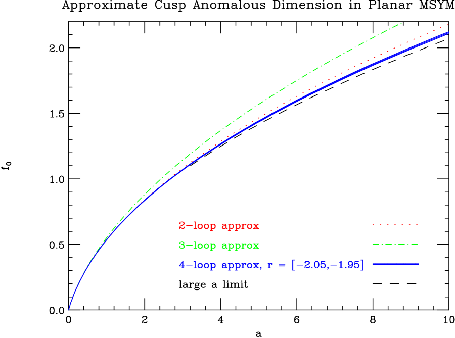
Figure 12: Approximations to the cusp anomalous dimension in planar MSYM based on the formula (82) and perturbative information through two loops (dotted line), three loops (dot-dash line) and four loops (solid line). Also shown is the strong-coupling prediction from string theory (dashed line).

In fig. 12 we plot these estimates as a function of the coupling, and we also display the strong-coupling limit (88) predicted by string theory. As noted above, the approximation (83) using only two-loop information works quite well, in fact better than the three-loop approximation (89). However, the behavior of the four-loop formula (93) is clearly extremely close to the string theory prediction. For this curve, or rather band, we have varied the parameter $r$ between $-2.05$ and $-1.95$, consistent with eq. (71).

We have constructed two further approximations by incorporating the knowledge of the precise strong-coupling coefficients. Matching the four-loop perturbative information and the leading strong-coupling coefficient gives the approximation

$$\hat{a}^{4} = (\tilde{f}_{0})^{4}+{2\over 3}\pi^{2}\ (\tilde{f}_{0})^{5}+{13\over 90}\pi^{4}\ (\tilde{f}_{0})^{6}+\left({23\over 1890}\pi^{6}-4(1+r)\zeta_{3}^{2}\right)(\tilde{f}_{0})^{7}+16\ (\tilde{f}_{0})^{8}\,.$$

It has the weak-coupling expansion,

$$\tilde{f}_{0} = \hat{a}-{\pi^{2}\over 6}\ \hat{a}^{2}+{11\over 180}\pi^{4}\ \hat{a}^{3}-\left({73\over 2520}\pi^{6}-(1+r)\zeta_{3}^{2}\right)\hat{a}^{4}$$ (101)

$$\hskip 0.0pt\hbox{}+\left({4747\over 302400}\pi^{8}-{3\over 2}(1+r)\pi^{2}\zeta_{3}^{2}-4\right)\hat{a}^{5}$$

$$\hskip 0.0pt\hbox{}-\left({5023\over 544320}\pi^{10}-{19\over 12}(1+r)\pi^{4}\zeta_{3}^{2}-{20\over 3}\pi^{2}\right)\hat{a}^{6}+\ldots\,,$$

as $$\hat{a}\to 0$$.

If we add the next-to-leading strong-coupling coefficient as another constraint, we obtain the approximation,

$$\hat{a}^{5} = (\tilde{f}_{0})^{5}+{5\over 6}\pi^{2}\ (\tilde{f}_{0})^{6}+{\pi^{4}\over 4}\ (\tilde{f}_{0})^{7}+\left({17\over 504}\pi^{6}-5(1+r)\zeta_{3}^{2}\right)(\tilde{f}_{0})^{8}$$ (102)

$$\hskip 0.0pt\hbox{}+{240\,\ln 2\over\pi}\ (\tilde{f}_{0})^{9}+32\ (\tilde{f}_{0})^{10}\,,$$

with the weak-coupling expansion,

$$\tilde{f}_{0} = \hat{a}-{\pi^{2}\over 6}\ \hat{a}^{2}+{11\over 180}\pi^{4}\ \hat{a}^{3}-\left({73\over 2520}\pi^{6}-(1+r)\zeta_{3}^{2}\right)\hat{a}^{4}$$ (103)

$$\hskip 0.0pt\hbox{}+\left({727\over 45360}\pi^{8}-{5\over 3}(1+r)\pi^{2}\zeta_{3}^{2}-{48\,\ln 2\over\pi}\right)\hat{a}^{5}$$

$$\hskip 0.0pt\hbox{}-\left({13387\over 1360800}\pi^{10}-{341\over 180}(1+r)\pi^{4}\zeta_{3}^{2}-88\,\pi\,\ln 2+{32\over 5}\right)\hat{a}^{6}+\ldots\,,$$

as $$\hat{a}\to 0$$.

We may also use the improved approximation (102) to determine subleading terms in the strong-coupling expansion. We have

$$\tilde{f}_{0} = \sqrt{{\hat{a}\over 2}}\ -\ {3\ln 2\over 4\pi}\ -\ \Bigl{(}{17\over 161280}\pi^{6}-{81\over 32\pi^{2}}\ln^{2}2-{1\over 64}(1+r)\zeta_{3}^{2}\Bigr{)}\sqrt{{2\over\hat{a}}}\ +\ {\cal O}(\hat{a}^{-1})\,.~{}~{}~{}~{}$$ (104)

For $r=-2$, this expression evaluates to

$$\tilde{f}_{0} \approx \sqrt{{\hat{a}\over 2}}\ -\ 0.16548\ -\ 0.000693\ \sqrt{{2\over\hat{a}}}\ +\ {\cal O}(\hat{a}^{-1})\,.$$ (105)

The first two numerical coefficients automatically reproduce the input StrongCouplingLeadingGKP ; Kruczenski ; Makeenko ; StrongCouplingSubleading from string theory, eq. (88), so the content of this equation is in the coefficient of $\sqrt{2/\hat{a}}$. Quite interestingly, this coefficient is very small, suggesting that it may even vanish in the exact expression. It is an intriguing question whether such a tiny or vanishing result could be obtained from string theory.

We plot these two approximations, for $r=-2$, along with the four-loop approximation (93), in fig. 13. Obviously, they are extremely close to one another. As a measure of that, the values they predict for the five-loop planar cusp anomalous dimension (for $r=-2$) are 167.03, 166.34 and 165.25, corresponding to the three approximations in eqs. (94), (101) and (103). We expect the last of these numbers to be the most accurate, given that eq. (103) uses all available information at both strong and weak coupling.

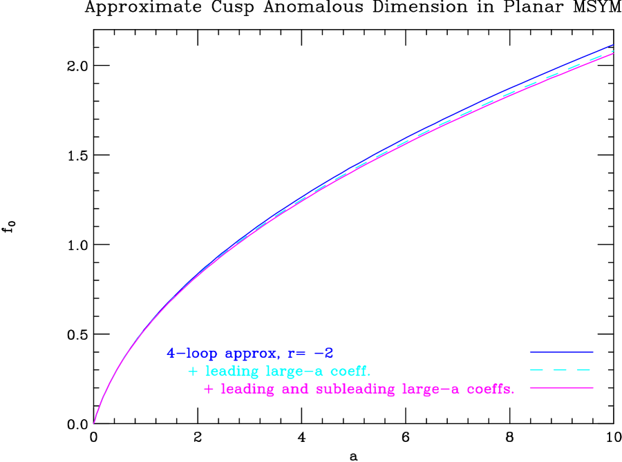
Figure 13: Approximations to the cusp anomalous dimension in planar MSYM based on the formula (82), four-loop perturbative information, and zero, one or two constants from the strong-coupling expansion.

Can we use these approximations to guide corrections to the ES prediction at higher loops? As a first step, consider the five-loop ES prediction in eq. (6). The ES numerical value is $131.22$, which disagrees significantly with the prediction of our approximate formula (103). However, we can modify the five-loop ES prediction (6) in a manner analogous to the modification required at four loops to fit the value $r=-2$. We flip the signs of the terms containing $\zeta_{n}$ values for odd $n$, and leave untouched the terms containing only even $\zeta$ values (those terms containing only $\pi$’s and rational numbers). Then the terms containing $\zeta_{3}$ and/or $\zeta_{5}$ in the five-loop coefficient in eq. (6) acquire the same sign as the $\pi^{8}$ term, instead of the opposite sign, giving an analytic expression through five loops:

$$f_{0}^{\rm modified}(\hat{a}) = \hat{a}-{\pi^{2}\over 6}\,\hat{a}^{2}+{11\over 180}\pi^{4}\,\hat{a}^{3}-\Bigl{(}{73\over 2520}\,\pi^{6}+\zeta_{3}^{2}\Bigr{)}\hat{a}^{4}$$ (106)

$$\hskip 56.9055pt\hbox{}+\Bigl{(}{887\over 56700}\,\pi^{8}+{\pi^{2}\over 3}\,\zeta_{3}^{2}+10\,\zeta_{3}\,\zeta_{5}\Bigr{)}\hat{a}^{5}+\ \cdots\,.$$

The numerical value of the five-loop coefficient in eq. (106), $165.65$, agrees with the five-loop coefficient in our approximate formula (103) to a remarkable 0.25%. This excellent agreement in turn reinforces the notion that $r=-2$ gives the correct analytical value of the four-loop coefficient. (We remark that a similar procedure at three loops, using the approximation (82) for $n=4$ and incorporating the two leading strong-coupling coefficients, works very well to estimate the next perturbative term: It predicts a four-loop coefficient of 30.22, which compares nicely with our result (66).)

We now continue this procedure to higher loops, comparing various predictions to our approximate formula. To obtain the ES prediction to higher-loop order, we use the integral equation from which eq. (6) is derived EdenStaudacher ,

$$f(\hat{a})\ =\ \hat{a}-4\,\hat{a}^{2}\int_{0}^{\infty}dt\,\hat{\sigma}(t)\,{J_{1}(\sqrt{2\hat{a}}\,t)\over\sqrt{2\hat{a}}\,t}\,,$$ (107)

where the fluctuation density $\hat{\sigma}(t)$ is obtained by solving the integral equation,

$$\hat{\sigma}(t)={t\over e^{t}-1}\Biggl{[}{J_{1}(\sqrt{2\hat{a}}\,t)\over\sqrt{2\hat{a}}\,t}-2\,\hat{a}\int_{0}^{\infty}dt^{\prime}\hat{K}(\sqrt{2\hat{a}}\,t,\sqrt{2\hat{a}}\,t^{\prime})\,\hat{\sigma}(t^{\prime})\Biggr{]}\,,$$ (108)

with the kernel,

$$\hat{K}(t,t^{\prime})={J_{1}(t)J_{0}(t^{\prime})-J_{0}(t)J_{1}(t^{\prime})\over t-t^{\prime}}\,,$$ (109)

where $J_{0}$ and $J_{1}$ are standard Bessel functions.

Solving this equation perturbatively through 12 loops, we find the numerical values of the ES prediction to be,

$$f_{0}^{\rm ES} = \hat{a}-1.6449\,\hat{a}^{2}+5.9528\,\hat{a}^{3}-26.405\,\hat{a}^{4}+131.22\,\hat{a}^{5}-705.54\,\hat{a}^{6}$$ (110)

$$\hbox{}+4021.9\,\hat{a}^{7}-23974.\,\hat{a}^{8}+1.4800\,10^{5}\,\hat{a}^{9}-9.3958\,10^{5}\,\hat{a}^{10}$$

$$\hbox{}+6.1024\,10^{6}\,\hat{a}^{11}-4.0387\,10^{7}\,\hat{a}^{12}+\cdots\,,$$

as $$\hat{a}\to 0$$.

The values in eq. (110) may be contrasted to the ones obtained from the weak coupling expansion of our approximate formula (102) (with $r=-2$),

$$f_{0}^{\rm approx} = \hat{a}-1.6449\,\hat{a}^{2}+5.9528\,\hat{a}^{3}-29.295\,\hat{a}^{4}+165.25\,\hat{a}^{5}-1002.7\,\hat{a}^{6}$$ (111)

$$\hbox{}+6379.3\,\hat{a}^{7}-41997.\,\hat{a}^{8}+2.8371\,10^{5}\,\hat{a}^{9}-1.9555\,10^{6}\,\hat{a}^{10}$$

$$\hbox{}+1.3699\,10^{7}\,\hat{a}^{11}-9.7237\,10^{7}\,\hat{a}^{12}+\cdots\,,$$

as $$\hat{a}\to 0$$.

The agreement between eqs. (110) and (111) at five loops and beyond is rather poor. This disagreement is not surprising, given that the ES four-loop value, used as input into our approximate formula (111), differs significantly from our calculation.

We have evaluated further terms in the weak-coupling expansion of our approximate formula (102), up to 75 loops. The ratio of the $n^{\rm th}$ term to the $(n-1)^{\rm st}$ term in the series slowly settles down to a value near $(-8)$ — at 75 loops it is $(-7.95)$ — suggesting a radius of convergence of $1/8$, and a nearest singularity on the negative real axis at $\hat{a}_{c}=-1/8$. This value does appear to agree with the location of the nearest singularity in the original ES equation LipatovPotsdam ; BESNew .

What happens if we generalize the four- and five-loop sign flips in the ES prediction, and require that all contributions at a given loop order come in with the same sign? Doing so, we obtain,

$$f_{0}^{\rm modified\ ES} = \hat{a}-1.6449\,\hat{a}^{2}+5.9528\,\hat{a}^{3}-29.295\,\hat{a}^{4}+165.65\,\hat{a}^{5}-1007.2\,\hat{a}^{6}$$ (112)

$$\hbox{}+6404.7\,\hat{a}^{7}-42020.\,\hat{a}^{8}+2.8223\,10^{5}\,\hat{a}^{9}-1.9307\,10^{6}\,\hat{a}^{10}$$

$$\hbox{}+1.3406\,10^{7}\,\hat{a}^{11}-9.4226\,10^{7}\,\hat{a}^{12}+\cdots\,,$$

as $$\hat{a}\to 0$$.

This modified formula is much closer to our approximate expression (111), differing even at 12 loops by only 3 percent. Of course, we have no reason to expect this naive modification of signs in the ES formula to be correct to all loop orders, though it appears to get the numerically largest contributions correct. Indeed, if we use this series to systematically construct KLV approximations with larger values of $n$ in eq. (82) as more terms are kept, the large $\hat{a}$ coefficients do not settle to the string values (87). For example, using the weak-coupling series (112) up to eight loops as input to the KLV approximation (82) with $n=7$ leads to a prediction at strong coupling,

$$\tilde{f}_{0} \approx 0.95968\,\sqrt{{\hat{a}\over 2}}\ -\ 0.081182\ +\ {\cal O}(\hat{a}^{-1/2})\,.$$ (113)

which compares poorly with either the string result (88) or with the four-loop prediction (97). It is noteworthy that the series (112) corresponds to the contemporaneous proposal in ref. BESNew . (We have checked agreement through 30 loops.) In order to improve the agreement of the higher-loop KLV approximations with the string theory strong-coupling coefficients, further modifications to the proposal are needed. Similar conclusions follow from the investigation of a sequence of Padé approximants, as discussed below.

The surprisingly good agreement of eqs. (111) and (112) does, however, suggest that a simple repair of the integral equation is possible. As a trivial example, by modifying the kernel in eq. (108) to $\hat{K}(\sqrt{2\hat{a}}\,t,-\sqrt{2\hat{a}}\,t^{\prime})$, we obtain

$$f_{0}^{\rm modified\ K} = \hat{a}-1.6449\,\hat{a}^{2}+5.9528\,\hat{a}^{3}-29.295\,\hat{a}^{4}+165.65\,\hat{a}^{5}-1011.9\,\hat{a}^{6}$$ (114)

$$\hbox{}+6490.0\,\hat{a}^{7}-43050.\,\hat{a}^{8}+2.9271\,10^{5}\,\hat{a}^{9}-2.0282\,10^{6}\,\hat{a}^{10}$$

$$\hbox{}+1.4265\,10^{7}\,\hat{a}^{11}-1.0156\,10^{8}\,\hat{a}^{12}+\cdots\,,$$

as $$\hat{a}\to 0$$.

which is in fairly good agreement with our approximate result. Although this ad hoc modification should only be taken as an illustration, it does show how one can use our approximate formula (111) to guide corrections to the ES integral equation. (It also suffers from the problem that strong-coupling extrapolations do not match the string values.) A proposed modification of the integral equation, valid through ${\cal O}(\hat{a}^{2})$ and leading to a modification in the anomalous dimension at ${\cal O}(\hat{a}^{4})$, is given in eqs. (89) and (91) of ref. EdenStaudacher . The choice $\beta=\zeta_{3}$ corresponds to $r=-2$ in eq. (70), as can be seen from eq. (92) of the same reference. This is also the choice preferred by crossing symmetry in the strong-coupling limit of the dressing factor, within the family of modifications newly studied in ref. BESNew .

It is useful to investigate other approximation schemes, to make sure that our results are not significantly biased by the form of the KLV approximate formula (82). A well-known method for incorporating information from different expansion regions — here from both weak and strong coupling — is that of Padé approximants, which fit a function to a ratio of polynomials in a suitable variable. In the complex $\hat{a}$ plane, we expect that $f_{0}(\hat{a})$ has poles or branch cuts. As discussed earlier, there is evidence from the behavior of the KLV approximation and the ES kernel that the singularity nearest the origin is at $\hat{a}_{c}=-1/8$. For the purposes of constructing the Padé approximant, however, we will model the singularities by a branch cut terminating on the negative real axis at the point $-\xi^{2}/8$. This assumption leads us to introduce a variable $u\equiv\sqrt{1+8\hat{a}/\xi^{2}}$, and define the $[(m+1)/m]$ Padé approximant by

$$f_{0}^{[(m+1)/m]}(u)=(u-1){N_{0}+N_{1}\,u+\ldots+N_{m}\,u^{m}\over 1+D_{1}\,u+\ldots+D_{m}\,u^{m}}\,.$$ (115)

The relative degrees of the numerator and denominator polynomials are fixed by the strong-coupling requirement $f_{0}\sim\sqrt{\hat{a}}\sim u$. The factor of $(u-1)$ comes from the vanishing of $f_{0}$ at $\hat{a}=0$. The remaining $2m+1$ constants can be fixed by perturbative data, or by a mix of weak- and strong-coupling data. Note that when $m$ increases by 1, two more input numbers are required.

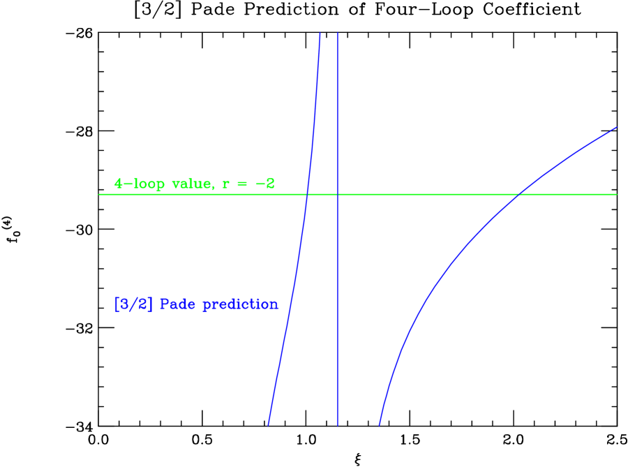
Figure 14: Value estimated for the four-loop cusp anomalous dimension $f_{0}^{(4)}$ by the $[3/2]$ Padé approximant (116), as a function of the parameter $\xi$ controlling the point at which the cut is assumed to terminate, $\hat{a}=-\xi^{2}/8$.

Consider first the $[3/2]$ Padé approximant,

$$f_{0}^{[3/2]}(u)=(u-1){N_{0}+N_{1}\,u+N_{2}\,u^{2}\over 1+D_{1}\,u+D_{2}\,u^{2}}\,,$$ (116)

which is implicitly a function of $\xi$, which parametrizes the location of the cut termination on the negative real axis. We solve for $N_{0}$, $N_{1}$, $N_{2}$, $D_{1}$ and $D_{2}$ as a function of $\xi$, using the two strong-coupling coefficients in eq. (87), plus the one-, two- and three-loop coefficients. We then expand the result in $\hat{a}$ in order to estimate the four-loop coefficient. This procedure will give us information about $\xi$. The four-loop coefficient is plotted in fig. 14. The value $\xi=1$ is picked out rather clearly by this plot, as the (approximate) first location where the curve crosses the value $f_{0}^{(4)}=-(73\,\pi^{6}/2520+\zeta_{3}^{2})=-29.2947$ (for $r=-2$). At $\xi=1$, formula (116) predicts $-29.521$. The second crossing is a spurious feature of the Padé, and the third crossing, near $\xi=2$, is highly implausible, based on the strong growth in the perturbative coefficients already at four loops, not to mention at higher orders in the KLV approximate formulas.

In fig. 15 we plot the ratio of the $[3/2]$ Padé to the KLV approximate formula (102), for various values of $\xi$ near 1 that produce four-loop coefficients that are not too far from $-29.2947$. Except for the pathological case of $\xi=1.05$, all the ratios are within about 1% of unity. For the preferred value of $\xi=1$, the $[3/2]$ Padé agrees with the KLV approximate formula everywhere to within about 0.1%. We also investigated the $[4/3]$ Padé, for $\xi=1$. This approximant requires two more input terms, namely the four- and five-loop coefficients. We used the “sign-flipped” values in eq. (106). The resulting expression predicts the six-loop coefficient to be $-1005.5$, in quite good agreement with the value of $-1002.7$ in eq. (111). On other hand, a plot of this function reveals a singularity on the positive real axis, at $u=4.791$, which is an artifact of a positive root to the cubic denominator polynomial. (The quadratic denominator polynomial in the $[3/2]$ Padé for $\xi=1$ has complex roots, relatively far from the real axis.) We also constructed a sequence of Padé approximants (115) to see how the strong-coupling coefficients are predicted by the proposed sign-flipped sequence (106). As with the KLV approximation, we do not find any convergence to the string values (87). For example, the $[4/3]$ Padé, based on the first seven loops in eq. (106), estimates

$$\tilde{f}_{0} \approx 0.95696\,\sqrt{{\hat{a}\over 2}}\ -\ 0.061164\ +\ {\cal O}(\hat{a}^{-1/2})\,,$$ (117)

which is close to the KLV estimation (113), and significantly different from the string values.

In summary, the different nature, yet very similar numerical results from the Padé approximation method gives us confidence that the KLV approximation (102) is good to better than a percent for all values of the coupling. It also gives confirming evidence that the singularity nearest the origin is located at $\hat{a}_{c}=-1/8$.

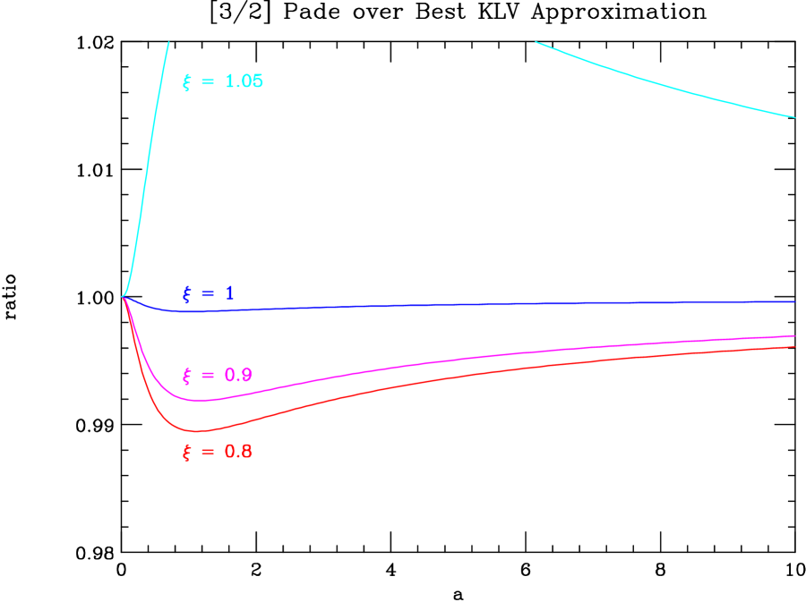
Figure 15: Ratio of the $[3/2]$ Padé approximant (116), as a function of the parameter $\xi$, to the KLV approximate formula (102), as a function of the coupling $\hat{a}$.

VIII Analysis and Conclusions

Using unitarity, we constructed the planar four-loop four-gluon amplitude in MSYM, and verified the structure of its infrared divergences through $1/\epsilon^{2}$. At order $1/\epsilon^{2}$ we were able to numerically test the prediction of Eden and Staudacher for the four-loop cusp anomalous dimension. Our result disagrees with their predictions. Using an approximate interpolating formula due to Kotikov, Lipatov and Velizhanin KLV , with the first four loop orders as input, we are able to estimate the first two coefficients of the strong-coupling expansion, coming to within 2.6 and 5 percent of the string theory prediction. Improving the approximate formula by using the string predictions as additional input, we obtain a formula for the cusp anomalous dimension which we expect to be valid for all couplings, to better than one percent. We have confirmed this using Padé approximations. Not surprisingly, given the disagreement at four loops, at higher orders the weak-coupling expansion of our approximate formula (102) has large disagreements with the ES prediction (110).

There are a number of conceivable reasons for the discrepancy at four loops, which we shall examine briefly in turn:

• Different definition of the coupling $g$.

• Difference between the cusp anomalous dimension defined for space-like vs. time-like kinematics.

• Breakdown of integrability.

• The wrapping problem.

• The dressing factor.

We expect the latter reasons to be more likely than the former.

In principle our result could differ from the ES result simply because we are expanding in coupling constants that differ beginning at three loops, say $\hat{a}^{\prime}=\hat{a}+x_{0}\,\zeta_{3}^{2}\,\hat{a}^{4}$ for the appropriate value of $x_{0}$. We use the classical coupling as our expansion parameter, so if this explanation is correct, the asymptotic Bethe ansatz would have to be using a different coupling. For example, in the magnon dispersion relation, discussed in eq. (2.18) of ref. BeisertDynamic , a parameter is adjusted to match the perturbative coupling of MSYM, via the relation $\alpha\beta=\hat{a}/2$. (Here $\alpha$ and $\beta$ describe the action of two central charges adjoined to an SU$(2|2)$ algebra acting on the spin chain.) If this simple substitution were to have corrections starting at order $\hat{a}^{4}$, it would lead to a four-loop discrepancy between the ES prediction from integrability and our direct calculation in MSYM.

Suppose our result and the ES result corresponded to cusp anomalous dimensions of different signature, i.e. one space-like and one time-like. Could this difference account for the different values? According to the results of Dokhshitzer, Marchesini and Salam DMS , it cannot, because the leading large-$x$ limits of the space-like and time-like DGLAP kernels should be identical, to all loop orders.

Integrability of the dilatation operator, interpreted as a spin model Hamiltonian, has not been proven to hold to all orders. However, the fact that there are very similar integrable structures at very strong gauge coupling — in the classical sigma model BPR and even in its quantum corrections Berkovits — suggests that integrability should persist.

Generically, a wrapping problem can occur if one tries to apply a Bethe ansatz solution for a spin-interaction that has longer range than the number of spin sites, which is equal to the twist $J$. Because the range of the interaction increases with the loop order, at fixed $J$ this problem becomes more severe with increasing loop order. It may well be that the wrapping problem prevents the asymptotic Bethe ansatz from being applied to short (twist-two) operators, even if it can be used for longer ones. The wrapping problem is generically supposed to arise at order $\hat{a}^{J-2}$ for operators of twist $J$. It is only other symmetries that protect the one-, two- and three-loop cusp anomalous dimensions from being affected by the wrapping problem.

It is quite possible that the discrepancy is resolved by the so-called “dressing factor”, an overall phase for the AdS/CFT $S$-matrix, which is consistent with integrability, the PSU$(2,2|4)$ symmetry, crossing symmetry, etc. The strong-coupling expansion of the dressing factor is known to be nontrivial. Indeed, the first two terms in the semi-classical expansion of the dressing factor on the string side have been worked out AFS04 ; OtherDressing ; HernandezLopez . There have also been very interesting recent analyses of the properties of the dressing factor under the worldsheet crossing symmetry JanikCrossing ; BHL . However, it remains unclear at which order in the weak-gauge-coupling expansion the dressing factor becomes non-trivial. If the reason for the discrepancy is indeed the dressing factor, then we now know it begins at four loops.

Eden and Staudacher made a specific proposal for modifying the asymptotic Bethe ansatz. They proposed a dressing factor containing a parameter $\beta$, thereby modifying the kernel of their integral equation. This leads to a shift in the four-loop cusp anomalous dimension proportional to $\beta$. If this proposal is correct, we determine the value of this parameter to be close to, if not exactly, $\beta=\zeta_{3}$.

Anomalous dimensions of many other classes of operators are linked through the PSU$(2,2|4)$ symmetry, and are therefore affected by a nontrivial dressing factor. As just one example, the anomalous dimension of the operator ${\cal O}\equiv\,{\rm Tr}(X^{2}Z^{3})+\ldots$, where $X$ and $Z$ are two of the three complex scalar fields in MSYM, is altered by an amount proportional to $\beta$, to have the form EdenStaudacher ,

$$4\hat{a}-6\,\hat{a}^{2}+17\,\hat{a}^{3}-\biggl{(}{115\over 2}+8\,\beta\biggr{)}\hat{a}^{4}+\cdots\,.$$ (118)

Thus the Eden–Staudacher proposal for the resolution of the discrepancy could be tested by a direct computation of the four-loop anomalous dimension of ${\cal O}$. For $\beta=\zeta_{3}$, it would appear to result in a non-uniform transcendentality for this quantity EdenStaudacher . (A caveat is that one needs to account also for the transcendentality assignment of harmonic sums KLOV , which are sums of rational numbers.) As pointed out by Eden and Staudacher, a nonzero value of $\beta$, through its effect on the anomalous dimension of ${\cal O}$, apparently rules out the Hubbard model Hamiltonian as a candidate for the $SU(2)$ dilatation operator beyond three loops RSS .

The Eden–Staudacher modification is the lowest-order term of a general form for the dressing factor $S_{12}=\exp(2i\theta(x_{1},x_{2}))$, with

$$\theta(x_{k},x_{j})=\sum_{r=2}^{\infty}\sum_{v=r+1}^{\infty}c_{r,v}\bigl{(}q_{r}(x_{k})q_{v}(x_{j})-q_{v}(x_{k})q_{r}(x_{j})\bigr{)}\,,$$ (119)

suggested in the literature AFS04 ; OtherDressing ; BeisertKlose ; BeisertInvariant ; BeisertDynamic ; BeisertPhase ; BHL . In this equation, the $q_{r}$ are the spin-chain charges,

$$q_{r}(x_{k})={i\over r-1}\biggl{(}{1\over(x^{+}_{k})^{r-1}}-{1\over(x^{-}_{k})^{r-1}}\biggr{)}\,,$$ (120)

and the $x^{\pm}_{i}$ are rapidities entering into the Bethe ansatz by which the spin-chain has been solved at lower orders.

All known quantities, anomalous dimensions or amplitudes, in the ${\cal N}=4$ supersymmetric theory, have a uniform transcendentality. That is, all polylogarithms or zeta constants at a given order in the perturbative expansion have the same polylog weight or transcendentality. The ES proposal deviates from this observed property in some quantities, such as eq. (118).

Is the dressing phase in eq. (119) general enough to accommodate our expectations for the ${\cal N}=4$ theory? As noted by Eden and Staudacher, maintaining uniform transcendentality with purely rational coefficients requires every power of $t$ or $t^{\prime}$ in their integral equation to come along with a power of the coupling $g$. Now, the coefficient of the $\zeta_{3}^{2}$ terms, which we wish to modify, arises from terms in the kernel proportional to $tt^{\prime}$. This term is odd in $t^{\prime}$. Such a term cannot arise from Fourier transforming a lone charge $q$, because we are interested in symmetric densities, and hence will ultimately take the symmetric part of this transform. The symmetric part is either zero (for $q_{r}$ with $r$ odd) or a symmetric function of $t^{\prime}$. In eq. (119), every term is linear in a charge $q(x_{j})$, and so it cannot lead to the modifications we need. We must therefore seek a more general dressing factor, or else introduce non-rational coefficients.

Very interestingly, in a contemporaneous paper, Beisert, Eden and Staudacher BESNew have done just the latter, in such a way that, at least for the anomalous dimension under consideration, uniform transcendentality is maintained. This leads to a modified integral equation of the ES type for the cusp anomalous dimension. At four loops the resulting anomalous dimension is in complete agreement with our direct computation of this quantity. Their proposal is compatible with integrability and with the KLOV transcendentality principle for the cusp anomalous dimension, and violates perturbative Berenstein-Maldacena-Nastase (BMN) scaling BMN starting at four loops. At five loops their proposal also matches our prediction of this coefficient, given in eq. (106), based on using both KLV KLV and Padé approximations. At higher-loop orders, their proposal corresponds to eq. (112) and appears to properly incorporate the numerically largest contributions. That is, it matches reasonably well our approximate expression (111). However, we find that successive KLV and Pade approximations, based on truncations at increasingly higher orders through 13 and 11 loops respectively, do not match the strong-coupling string results. This indicates a tension between the weak- and strong-coupling results, and suggests to us that further modifications may be necessary. The question merits further study.

We remark that, assuming the KLOV conversion principle, our result for the leading-color four-loop cusp anomalous dimension also predicts a piece of the corresponding result in QCD. Which piece? At three loops and below, the QCD result is a polynomial in the $SU(N_{c})$ Casimir operators $C_{A}$ and $C_{F}$, while the MSYM result is composed solely of $C_{A}=N_{c}$, so it has no subleading-color terms. The MSYM result provides one constraint on the leading-transcendentality parts of the coefficients of the color factors in QCD, such that, after the group theory Casimirs have been set to the values $C_{F}=C_{A}=N_{c}$, the leading-color terms are equal to the MSYM result. Starting at four loops, however, there are color factors that cannot be reduced to polynomials in $C_{A}$ and $C_{F}$. The relevant color factors are those of $L$-loop propagator diagrams.

In MSYM, any triangle subdiagram leads to a group-theory factor of $C_{A}$, times a lower-loop group-theory factor. So the question is, when do no-triangle propagator diagrams first appear? At three loops, there is one nonplanar no-triangle propagator diagram, but its color factor vanishes identically using the Jacobi identity (see e.g. ref. TwoLoopSplitting ). At four loops, fig. 6(d₅) illustrates the unique such planar graph (when the two pairs of external lines on the left and right sides of the graph are each replaced with single lines). There are a number of nonplanar graphs as well. Hence the cusp anomalous dimension in MSYM can now have subleading-color terms. Presumably the KLOV principle will apply with respect to the leading-color, planar terms, once the fermionic color factors in the QCD result are shifted from the fundamental to adjoint representation. But will it also apply to subleading-color terms? If conformal invariance is the main issue KLOV , then it should. But if planarity is important, perhaps it will not. Of course, the question is a moot one until the cusp anomalous dimension in QCD, and the subleading-color part of that in MSYM, are both known at four loops. Similar remarks apply to the four-loop form-factor quantity ${\cal G}_{0}^{(4)}$.

In order to confirm that the four-loop cusp anomalous dimension is given exactly by the ${\cal O}(\hat{a}^{4})$ term in eq. (106), it would be important to evaluate it analytically. To do so, the four-loop integrand (39) would have to be evaluated analytically through ${\cal O}(\epsilon^{-2})$ instead of only through ${\cal O}(\epsilon^{-4})$ as done here. It would also be extremely interesting to evaluate the four-loop integrand through ${\cal O}(\epsilon^{0})$, to explicitly check the four-loop iteration relation (32) for scattering amplitudes Iterate2 ; Iterate3 .

The program MB CzakonMB can be used to express the coefficients at each order in the Laurent expansion in $\epsilon$ as a sum of finite contour integrals. However, the number of such integrals increases rapidly with decreasing inverse power of $\epsilon$. This property, along with an increase in dimensionality of the integrals, makes it harder to compute the integrals purely numerically, requiring a substantial increase in computational resources for the same relative level of accuracy. For example, the order $\epsilon^{-2}$ term in $M_{4}^{(4)}$ in table 2 has a relative precision of $2\times 10^{-4}$, 40 times larger than that of the order $\epsilon^{-3}$ term, despite having had significantly more computing resources applied to it. Although a brute-force computation of the $1/\epsilon$ and $\epsilon^{0}$ terms could probably be completed with sufficient resources, it would be considerably lengthier than the present computation. Accordingly, we believe that additional analytic work would be rather desirable before proceeding further.

The information provided in this paper offers a guide to further progress in determining the integrable structure of planar MSYM, as well as in studying the transition from weak to strong coupling. For the cusp anomalous dimension, the striking match between the first two coefficients of the strong-coupling expansion, as estimated by us, using our four-loop result as input to the KLV approximation KLV , and as obtained from string theory StrongCouplingLeadingGKP ; Kruczenski ; Makeenko ; StrongCouplingSubleading , provides good evidence that we have an excellent numerical understanding of this anomalous dimension at any coupling. The same approximation strongly suggests that the correct analytic forms of the four- and five-loop perturbative coefficients are the ones given in eq. (106). These types of approximations can also be useful for checking whether a given ansatz for higher-order terms in the weak-coupling expansion are consistent with the known string theory strong-coupling results. This should help in finding the correct integral equation describing the MSYM cusp anomalous dimension. Another intriguing result from the extrapolation to strong coupling is that the next term in the expansion (${\cal O}(\hat{a}^{-1/2})$) should be very small and may even vanish. Finally, the remarkably good numerical properties of the approximate formulas indicate that the transition between weak and strong coupling is smooth for planar ${\cal N}=4$ super-Yang-Mills theory.

Appendix A Evaluating four-loop integrals by MB representation

To obtain Laurent expansions in $\epsilon$ for our integrals we use the Mellin–Barnes (MB) technique, which has been successfully applied in numerous calculations (see, e.g., refs. SmirnovDoubleBox ; Tausk ; SmirnovTripleBox ; Iterate3 ; TwoloopOffandMassive and chapter 4 of ref. Buch ). It relies on the identity

$$\frac{1}{(X+Y)^{\lambda}}=\int_{\beta-i\infty}^{\beta+i\infty}\frac{Y^{z}}{X^{\lambda+z}}\frac{\Gamma(\lambda+z)\Gamma(-z)}{\Gamma(\lambda)}\frac{\mbox{d}z}{2\pi i}\,,$$ (121)

where $-{\rm Re}\,\lambda<\beta<0$. This identity basically replaces a sum over terms raised to some power with a product of factors.

It is convenient to keep arbitrary powers of propagators and numerator factors in each of the MB representations. In this way, one can check the MB representations by setting some of the indices to zero, in order to obtain a simpler integral whose value is already known. Also, we can obtain the values of the two non-rung-rule integrals of fig. 4 from two of the rung-rule integrals of fig. 2 by setting some of the indices to zero.

We define a four-loop integral with general indices as,

$$F^{(x)}(a_{1},\ldots,a_{n_{i}};s,t;\epsilon) = (-ie^{\epsilon\gamma}\pi^{-d/2})^{4}\int{\mbox{d}^{d}p\,\mbox{d}^{d}r\,\mbox{d}^{d}u\,\mbox{d}^{d}v\over\prod_{j=1}^{n_{i}}(p_{j}^{2})^{a_{j}}}\,,$$ (122)

where $p,r,u,v$ are the four independent loop, $n_{i}$ the number of indices corresponding to the $p_{j}^{2}$ propagator and numerator factors in a given graph. For each graph $(x)$ the labels correspond to the propagator and numerator labels of fig. 2. In this notation a numerator factor is indicated by negative indices.

Experience shows that a minimal number of MB integrations for planar diagrams is achieved if one introduces MB integrations loop by loop, i.e. one derives a MB representation for a one-loop subintegral, inserts it into a higher two-loop integral, etc. This straightforward strategy provides the following MB representations for the Feynman integrals corresponding to graphs of fig. 2, with general powers of the propagators and irreducible numerators:

$$F^{\rm(a)}(a_{1},\ldots,a_{13};s,t;\epsilon)=\frac{e^{4\epsilon\gamma}\,(-1)^{a}(-s)^{8-a-4\epsilon}}{\prod_{j=2,5,7,9,11,12,13}\Gamma(a_{j})\Gamma(4-a_{9,11,12,13}-2\epsilon)}$$ (123)

$$\times\frac{1}{(2\pi i)^{11}}\int_{-i\infty}^{+i\infty}\ldots\int_{-i\infty}^{+i\infty}\prod_{j=1}^{11}\mbox{d}z_{j}\left(\frac{t}{s}\right)^{z_{7}}\frac{\Gamma(2-a_{9,12,13}-\epsilon-z_{1,2})\Gamma(2-a_{9,11,12}-\epsilon-z_{1,3})}{\Gamma(a_{10}-z_{2})\Gamma(a_{8}-z_{3})\Gamma(a_{6}-z_{5})\Gamma(a_{4}-z_{6})}$$

$$\times\frac{\Gamma(a_{9}+z_{1,2,3})\Gamma(a_{9,11,12,13}-2+\epsilon+z_{1,2,3})\Gamma(z_{10}-z_{4})\Gamma(z_{4}-z_{1})}{\Gamma(4-a_{5,8,10}-2\epsilon+z_{1,2,3})\Gamma(4-a_{4,6,7}-2\epsilon+z_{4,5,6})\Gamma(4-a_{1,2,3}-2\epsilon+z_{8,9,10})}$$

$$\times\frac{\Gamma(2-a_{5}-a_{8}-\epsilon+z_{1}+z_{3}-z_{4}-z_{6})\Gamma(a_{5,9,10}-2+\epsilon-z_{1,2,3}+z_{4,5,6})}{\Gamma(a_{3}-z_{9})\Gamma(a_{1}-z_{8})}$$

$$\times\Gamma(a_{12}+z_{1})\Gamma(a_{2}+z_{7})\Gamma(z_{7}-z_{10})\Gamma(2-a_{6,7}-\epsilon-z_{8,10}+z_{4,5})\Gamma(2-a_{1,2}-\epsilon+z_{8,10}-z_{7})$$

$$\times\Gamma(2-a_{4,7}-\epsilon-z_{9,10}+z_{4,6})\Gamma(a_{1,2,3}-2+\epsilon+z_{7}-z_{8,9,10})\Gamma(2-a_{2,3}-\epsilon+z_{9,10}-z_{7})$$

$$\times\Gamma(a_{7}+z_{8,9,10})\Gamma(2-a_{5,10}-\epsilon+z_{1,2}-z_{4,5})$$

$$\times\Gamma(a_{5}+z_{4}+z_{5}+z_{6})\Gamma(a_{4,6,7}-2+\epsilon-z_{4,5,6}+z_{8,9,10})\prod_{j=2,3,5,6,7,8,9}\Gamma(-z_{j})\;,$$

$$F^{\rm(b)}(a_{1},\ldots,a_{14};s,t;\epsilon)=\frac{e^{4\epsilon\gamma}\,(-1)^{a}(-s)^{8-a-4\epsilon}}{\prod_{j=2,4,5,6,7,9,12}\Gamma(a_{j})\Gamma(4-a_{4,5,6,7}-2\epsilon)}$$ (124)

$$\times\frac{1}{(2\pi i)^{12}}\int_{-i\infty}^{+i\infty}\ldots\int_{-i\infty}^{+i\infty}\prod_{j=1}^{12}\mbox{d}z_{j}\left(\frac{t}{s}\right)^{z_{9,12}}\frac{\Gamma(8-a+a_{12}-4\epsilon-z_{9,12})}{\Gamma(10-a-5\epsilon-z_{9})\Gamma(a_{13}-z_{10})\Gamma(a_{1}-z_{2})}$$

$$\times\frac{\Gamma(a_{9}+z_{9,10})\Gamma(a_{13}-z_{10}+z_{12})\Gamma(2-a_{5,6,7}-\epsilon-z_{1,2,4})\Gamma(2-a_{4,5,7}-\epsilon-z_{1,3})}{\Gamma(4-a_{1,2,3}-2\epsilon+z_{1,2,3})\Gamma(a_{14}-z_{4,8,11})\Gamma(a_{8}-z_{6})\Gamma(a_{3}-z_{3})}$$

$$\times\frac{\Gamma(a_{7}+z_{1,2,3})\Gamma(a_{4,5,6,7}-2+\epsilon+z_{1,2,3,4})\Gamma(z_{9,11}-z_{5})\Gamma(2-a_{12,13,14}-\epsilon+z_{4,8,10,11}-z_{12})}{\Gamma(a_{10}-z_{7})\Gamma(4-a_{8,9,10}-2\epsilon+z_{5,6,7})}$$

$$\times\frac{\Gamma(a_{5}+z_{1,4})\Gamma(2-a_{2,3}-\epsilon+z_{1,3}-z_{5,7})\Gamma(a_{2}+z_{5,6,7})\Gamma(a_{14}-z_{4,8,11}+z_{12})}{\Gamma(a_{1,2,3,4,5,6,7,8,9,10,11}-6+3\epsilon+z_{4,8,9,10,11})}$$

$$\times\Gamma(2-a_{1,2}-\epsilon+z_{1,2}-z_{5,6,8})\Gamma(z_{5,8}-z_{1})\Gamma(a_{1,2,3}-2+\epsilon-z_{1,2,3}+z_{5,6,7,8})$$

$$\times\Gamma(2-a_{8,9}-\epsilon+z_{5,6}-z_{9,10,11})\Gamma(2-a_{9,10}-\epsilon+z_{5,7}-z_{9})\Gamma(a-8+4\epsilon+z_{9,12})$$

$$\times\Gamma(a_{8,9,10}-2+\epsilon-z_{5,6,7}+z_{9,10,11})\prod_{j=2,3,4,6,7,8,9,10,11,12}\Gamma(-z_{j})\;,$$

$$F^{\rm(c)}(a_{1},\ldots,a_{14};s,t;\epsilon)=\frac{e^{4\epsilon\gamma}\,(-1)^{a}(-t)^{8-a-4\epsilon}}{\prod_{j=2,4,5,6,7,8,12}\Gamma(a_{j})\Gamma(4-a_{4,5,6,7}-2\epsilon)}$$ (125)

$$\times\frac{1}{(2\pi i)^{11}}\int_{-i\infty}^{+i\infty}\ldots\int_{-i\infty}^{+i\infty}\prod_{j=1}^{11}\mbox{d}z_{j}\left(\frac{s}{t}\right)^{z_{5,8,11}}\frac{\Gamma(a_{14}-z_{10}+z_{11})\Gamma(2-a_{4,5,7}-\epsilon-z_{1,3})}{\Gamma(a_{14}-z_{10})\Gamma(a_{1}-z_{2})\Gamma(4-a_{1,2,3}-2\epsilon+z_{1,2,3})}$$

$$\times\frac{\Gamma(2-a_{5,6,7}-\epsilon-z_{1,2,4})\Gamma(a_{5}+z_{1,4})\Gamma(a_{4,5,6,7}-2+\epsilon+z_{1,2,3,4})\Gamma(2-a_{2,3}-\epsilon+z_{1,3}-z_{5})}{\Gamma(8-a_{1,2,3,4,5,6,7,8,9,10,11}-4\epsilon-z_{5})\Gamma(a_{9}-z_{6})\Gamma(a_{10}-z_{4,7})\Gamma(a_{3}-z_{3})}$$

$$\times\frac{\Gamma(a_{2}+z_{5,6})\Gamma(2-a_{1,2}-\epsilon+z_{1,2}-z_{5,6,7})\Gamma(z_{5,7}-z_{1})\Gamma(a_{1,2,3}-2+\epsilon-z_{1,2,3}+z_{5,6,7})}{\Gamma(a_{1,2,3,4,5,6,7,11}-4+2\epsilon+z_{4,5,6,7})\Gamma(10-a-5\epsilon-z_{5,8})\Gamma(a_{13}-z_{9})}$$

$$\times\Gamma(6-a_{1,2,3,4,5,6,7,9,10,11}-3\epsilon-z_{5,8})\Gamma(8-a+a_{12}-4\epsilon-z_{5,8,11})\Gamma(a-8+4\epsilon+z_{5,8,11})$$

$$\times\Gamma(a_{10}+z_{8,10}-z_{4,7})\Gamma(a_{13}+z_{11}-z_{9})\Gamma(2-a_{8,9,10}-\epsilon+z_{4,6,7}-z_{8,9,10})\Gamma(a_{7}+z_{1,2,3})$$

$$\times\Gamma(2-a_{12,13,14}-\epsilon+z_{9,10}-z_{11})\Gamma(a_{9}-z_{6}+z_{8,9})\prod_{j=2}^{11}\Gamma(-z_{j})\;,$$

$$F^{\rm(d)}(a_{1},\ldots,a_{14};s,t;\epsilon)=\frac{e^{4\epsilon\gamma}\,(-1)^{a}(-s)^{8-a-4\epsilon}}{\prod_{j=2,4,5,6,7,9,12}\Gamma(a_{j})\Gamma(4-a_{4,5,6,7}-2\epsilon)}$$ (126)

$$\times\frac{1}{(2\pi i)^{14}}\int_{-i\infty}^{+i\infty}\ldots\int_{-i\infty}^{+i\infty}\prod_{j=1}^{14}\mbox{d}z_{j}\left(\frac{t}{s}\right)^{z_{14}}\frac{\Gamma(a_{12}+z_{11})\Gamma(a_{9}+z_{14})\Gamma(z_{14}-z_{11})}{\Gamma(a_{1}-z_{2})\Gamma(4-a_{1,2,3}-2\epsilon+z_{1,2,3})\Gamma(a_{13}-z_{5,10})}$$

$$\times\frac{\Gamma(2-a_{5,6,7}-\epsilon-z_{1,2,4})\Gamma(2-a_{4,5,7}-\epsilon-z_{1,3,5})\Gamma(a_{5}+z_{1,4,5})\Gamma(a_{4,5,6,7}-2+\epsilon+z_{1,2,3,4,5})}{\Gamma(a_{11}-z_{8})\Gamma(a_{8}-z_{4,9,12})\Gamma(8-a_{1,2,3,4,5,6,7,11,12,13,14}-4\epsilon-z_{4,6,7,9})\Gamma(a_{10}-z_{7,13})}$$

$$\times\frac{\Gamma(2-a_{9,10}-\epsilon+z_{7,11,13}-z_{14})\Gamma(2-a_{2,3}-\epsilon+z_{1,3}-z_{6,8,10})\Gamma(a_{2}+z_{6,7,8})\Gamma(a_{7}+z_{1,2,3})}{\Gamma(4-a_{8,9,10}-2\epsilon+z_{4,7,9,11,12,13})\Gamma(a_{1,2,3,4,5,6,7,14}-4+2\epsilon+z_{4,5,6,7,8,9,10})\Gamma(a_{3}-z_{3})}$$

$$\times\Gamma(a_{8,9,10}-2+\epsilon-z_{4,7,9,11,12,13}+z_{14})\Gamma(2-a_{1,2}-\epsilon+z_{1,2}-z_{6,7,9})$$

$$\times\Gamma(6-a_{1,2,3,4,5,6,7,11,12,14}-3\epsilon-z_{4,5,6,7,9,10,11,13})\Gamma(6-a_{1,2,3,4,5,6,7,12,13,14}-3\epsilon-z_{4,6,7,8,9,11,12})$$

$$\times\Gamma(2-a_{8,9}-\epsilon+z_{4,9,11,12}-z_{14})\Gamma(a_{1,2,3,4,5,6,7,11,12,13,14}-6+3\epsilon+z_{4,6,7,9,11,12,13})$$

$$\times\Gamma(z_{6,9,10}-z_{1})\Gamma(a_{1,2,3}-2+\epsilon-z_{1,2,3}+z_{6,7,8,9,10})$$

$$\times\Gamma(a_{1,2,3,4,5,6,7,14}-4+2\epsilon+z_{4,5,6,7,8,9,10,11,12,13})\prod_{j=2,3,4,5,6,7,8,9,10,12,13,14}\Gamma(-z_{j})\;,$$

$$F^{\rm(e)}(a_{1},\ldots,a_{15};s,t;\epsilon)=\frac{e^{4\epsilon\gamma}\,(-1)^{a}(-s)^{8-a-4\epsilon}}{\prod_{j=2,4,5,6,7,9,11}\Gamma(a_{j})\Gamma(4-a_{4,5,6,7}-2\epsilon))}$$ (127)

$$\times\frac{1}{(2\pi i)^{12}}\int_{-i\infty}^{+i\infty}\ldots\int_{-i\infty}^{+i\infty}\prod_{j=1}^{12}\mbox{d}z_{j}\left(\frac{t}{s}\right)^{z_{12}}\frac{\Gamma(a_{9}+z_{12})\Gamma(2-a_{5,6,7}-\epsilon-z_{1,2})\Gamma(a_{7}+z_{1,2,3})}{\Gamma(a_{10}-z_{11})\Gamma(a_{1}-z_{2})\Gamma(4-a_{1,2,3}-2\epsilon+z_{1,2,3})}$$

$$\times\frac{\Gamma(2-a_{4,5,7}-\epsilon-z_{1,3,4})\Gamma(a_{4,5,6,7}-2+\epsilon+z_{1,2,3,4})\Gamma(2-a_{1,2}-\epsilon+z_{1,2}-z_{5,6})}{\Gamma(a_{8}-z_{6,10})\Gamma(a_{13}-z_{7})\Gamma(a_{3}-z_{3})\Gamma(8-a_{1,2,3,4,5,6,7,11,12,13,14}-4\epsilon-z_{5,6})\Gamma(a_{12}-z_{4,8})}$$

$$\times\frac{\Gamma(a_{2}+z_{5,6,7})\Gamma(2-a_{2,3}-\epsilon+z_{1,3}-z_{5,7,8})\Gamma(z_{5,8}-z_{1})\Gamma(a_{1,2,3}-2+\epsilon-z_{1,2,3}+z_{5,6,7,8})}{\Gamma(a_{1,2,3,4,5,6,7,14}-4+2\epsilon+z_{4,5,6,7,8})\Gamma(a_{15}-z_{5,9})\Gamma(4-a_{8,9,10,15}-2\epsilon+z_{5,6,9,10,11})}$$

$$\times\Gamma(6-a_{1,2,3,4,5,6,7,12,13,14}-3\epsilon-z_{5,6,9,10})\Gamma(a_{8,9,10,15}-2+\epsilon-z_{5,6,9,10,11}+z_{12})$$

$$\times\Gamma(a_{15}+z_{12}-z_{5,9})\Gamma(2-a_{11,12,13}-\epsilon+z_{4,7,8}-z_{9,11})\Gamma(2-a_{9,10,15}-\epsilon+z_{5,9,11}-z_{12})$$

$$\times\Gamma(a_{1,2,3,4,5,6,7,11,12,13,14}-6+3\epsilon+z_{5,6,9,10,11})\Gamma(2-a_{8,9,15}-\epsilon+z_{5,6,9,10}-z_{12})$$

$$\times\Gamma(a_{5}+z_{1,4})\Gamma(a_{13}-z_{7}+z_{9,10,11})\Gamma(a_{12}-z_{4,8}+z_{9})\prod_{j=2}^{12}\Gamma(-z_{j})\;,$$

$$F^{\rm(f)}(a_{1},\ldots,a_{15};s,t;\epsilon)=\frac{e^{4\epsilon\gamma}\,(-1)^{a}(-s)^{8-a-4\epsilon}}{\prod_{j=1}^{8}\Gamma(a_{j})\Gamma(4-a_{1,2,3,4}-2\epsilon)\Gamma(4-a_{5,6,7,8}-2\epsilon)}$$ (128)

$$\times\frac{1}{(2\pi i)^{14}}\int_{-i\infty}^{+i\infty}\ldots\int_{-i\infty}^{+i\infty}\prod_{j=1}^{14}\mbox{d}z_{j}\left(\frac{t}{s}\right)^{z_{5,6}}\frac{\Gamma(2-a_{6,7,8}-\epsilon-z_{11,13})\Gamma(a_{8}+z_{11,14})}{\Gamma(a_{13}-z_{10,12})\Gamma(a_{11}-z_{14})\Gamma(a_{10}-z_{3,13})}$$

$$\times\frac{\Gamma(2-a_{5,6,8}-\epsilon-z_{11,12,14})\Gamma(a_{6}+z_{11,12,13})\Gamma(a_{13}+z_{1,2,3,4}-z_{10,12})\Gamma(a_{11}+z_{4,5}-z_{14})}{\Gamma(a_{14}-z_{7})\Gamma(a_{9}-z_{2,8})\Gamma(a_{12}-z_{9})\Gamma(6-a_{1,2,3,4,9,10,15}-3\epsilon+z_{1,2,3,4,11,13}-z_{7,9,10})}$$

$$\times\frac{\Gamma(a_{14}+z_{2,5}-z_{7})\Gamma(4-a_{5,6,7,8,11,13,14}-2\epsilon-z_{2,3,4,5,11,13}+z_{7,10})\Gamma(a_{9}-z_{2,8}+z_{6})}{\Gamma(a_{15}-z_{4,11})\Gamma(6-a_{5,6,7,8,11,12,13,14}-3\epsilon+z_{7,9,10}-z_{11,13})}$$

$$\times\frac{\Gamma(a_{15}-z_{4,11}+z_{6})\Gamma(2-a_{2,3,4}-\epsilon-z_{7,8,10})\Gamma(2-a_{9,10,15}-\epsilon+z_{2,3,4,8,11,13}-z_{6})}{\Gamma(a_{1,2,3,4}-2+\epsilon-z_{1}+z_{7,8,9,10})}$$

$$\times\Gamma(2-a_{1,2,4}-\epsilon-z_{7,9})\Gamma(a_{5,6,7,8,11,12,13,14}-4+2\epsilon+z_{1,2,3,4,5,11,13}-z_{7,9,10})$$

$$\times\Gamma(4-a_{1,2,3,4,9,15}-2\epsilon+z_{1,2,4,11}-z_{6,7,9,10})\Gamma(a_{4}+z_{7,9,10})\Gamma(a_{2}+z_{7,8})$$

$$\times\Gamma(2-a_{11,12,13,14}-\epsilon-z_{1,2,4,5}+z_{7,9,10,12,14})\Gamma(a_{1,2,3,4}-2+\epsilon+z_{7,8,9,10})$$

$$\times\Gamma(a_{1,2,3,4,9,10,15}-4+2\epsilon-z_{1,2,3,4,11,13}+z_{6,7,9,10})\prod_{j=1}^{14}\Gamma(-z_{j})\;,$$

where $a_{4,5,6,7}=a_{4}+a_{5}+a_{6}+a_{7}$, $a=\sum a_{i}$, $z_{11,12,13}=z_{11}+z_{12}+z_{13}$, etc.

From these general integrals, by choosing appropriate indices, we may then obtain the eight integrals that appear in the four-loop amplitude,

$${\cal I}^{\rm(a)} = s^{4}t\,F^{\rm(a)}(1,1,1,1,1,1,1,1,1,1,1,1,1;s,t;\epsilon)\,,$$ (129)

$${\cal I}^{\rm(b)} = st^{2}\,F^{\rm(b)}(1,1,1,1,1,1,1,1,1,1,-2,1,1,1;s,t;\epsilon)\,,$$ (130)

$${\cal I}^{\rm(c)} = s^{3}t\,F^{\rm(c)}(1,1,1,1,1,1,1,1,1,1,-1,1,1,1;s,t;\epsilon)\,,$$ (131)

$${\cal I}^{\rm(d)} = s^{3}t\,F^{\rm(d)}(1,1,1,1,1,1,1,1,1,1,1,1,1,-1;s,t;\epsilon)\,,$$ (132)

$${\cal I}^{\rm(e)} = s^{2}t\,F^{\rm(e)}(1,1,1,1,1,1,1,1,1,1,1,1,1,-1,-1;s,t;\epsilon)\,,$$ (133)

$${\cal I}^{\rm(f)} = \lim_{\eta\rightarrow 0}s^{2}t\,F^{\rm(f)}(1,1,1,1,1,1,1,1,1,1,1,1,1,-1+\eta,-1;s,t;\epsilon)\,,$$ (134)

$${\cal I}^{\rm(d_{2})} = s^{2}t\,F^{\rm(d)}(1,1,1,1,1,1,1,1,1,0,1,1,0,0;s,t;\epsilon)\,,$$ (135)

$${\cal I}^{\rm(f_{2})} = s^{2}t^{2}\,F^{\rm(f)}(1,1,1,1,1,1,1,1,1,1,1,1,0,0,0;s,t;\epsilon)\,.$$ (136)

For the case of integral $\rm(f)$, in order to obtain a valid analytic continuation to the region $\epsilon\rightarrow 0$ using MB CzakonMB , it turns out that we first need to perform an analytic continuation in one of the indices, by an auxiliary parameter $\eta$. After the analytic continuation we may set $\eta\rightarrow 0$.

Appendix B Harmonic polylogarithms

We express the leading poles in the integrals and the amplitudes in terms of harmonic polylogarithms (HPLs) HPL , generalizations of ordinary polylogarithms Lewin . Here we briefly summarize their definitions; see ref. HPL for a more complete treatment. Routines for numerically evaluating HPLs may be found in ref. HPL2 ; HPLMaitre .

The HPLs of weight $n$ are denoted by $H_{a_{1}a_{2}\ldots a_{n}}(x)\equiv H(a_{1},a_{2},\ldots,a_{n};x)$, with $a_{i}\in\{1,0,-1\}$. They are defined recursively by,

$$H_{a_{1}a_{2}\ldots a_{n}}(x)=\int_{0}^{x}\mbox{d}t\,f_{a_{1}}(t)H_{a_{2}\ldots a_{n}}(t)\,,$$ (137)

where

$$f_{\pm 1}(x) = {1\over 1\mp x}\,,\qquad f_{0}(x)={1\over x}\,,$$ (138)

$$H_{\pm 1}(x) = \mp\ln(1\mp x)\,,\qquad H_{0}(x)=\ln x\,,$$ (139)

provided that at least one of the indices $a_{i}$ is non-zero. For all $a_{i}=0$, one defines

$$H_{0,0,\ldots,0}(x)=\frac{1}{n!}\ln^{n}x\;.$$ (140)

For weight less than or equal to four, any HPL having only the parameters $a_{i}=0$ and $1$ can be expressed HPL in terms of the standard polylogarithms Lewin ,

$$\mathop{\rm Li}\nolimits_{n}(z) = \sum_{j=1}^{\infty}{z^{j}\over j^{n}}=\int_{0}^{z}{\mbox{d}t\over t}\mathop{\rm Li}\nolimits_{n-1}(t)\,,$$

$$\mathop{\rm Li}\nolimits_{2}(z) = -\int_{0}^{z}{\mbox{d}t\over t}\ln(1-t)\,,$$ (141)

with $n=2,3,4$, and where $z$ may take the values $x$, $1/(1-x)$, or $-x/(1-x)$. (For $n<4$, polylogarithm identities imply that not all values are required.) For the four-loop results presented in section VI.1 through ${\cal O}(\epsilon^{-4})$, we indeed need only $a_{i}\in\{0,1\}$, and weights up to four. In section VI.2, however, we give analytic results for lower-loop amplitudes at the symmetric point $(s,t)=(-1,-1)$ through ${\cal O}(\epsilon^{-2})$, in which we encounter weights up to six. In the Euclidean region for the planar four-point process, namely $s<0$, $t<0$, $u>0$, with the identification $x=-t/s$, the argument $x$ of the harmonic polylogarithms will be negative.

The HPLs obey sets of identities HPL that allow the removal of trailing zeroes from the string of parameters $a_{i}$. The remaining $H_{a_{1}a_{2}\ldots a_{n}}(x)$ with $a_{n}=1$ are well-behaved as $x\to 0$; in fact they all vanish there. Integrals appear in the MSYM amplitudes with both arguments $(s,t)$ and $(t,s)$, so we also need a set of identities relating harmonic polylogarithms with argument $x=-t/s$ to those with argument $y=-s/t=1/x$. These identities are given in refs. HPL . A few directly relevant examples may be found in the first appendix of ref. Iterate3 .

References

• (1) J. M. Maldacena, Adv. Theor. Math. Phys. 2, 231 (1998) [Int. J. Theor. Phys. 38, 1113 (1999)] [hep-th/9711200];
S. S. Gubser, I. R. Klebanov and A. M. Polyakov, Phys. Lett. B 428, 105 (1998) [hep-th/9802109];
O. Aharony, S. S. Gubser, J. M. Maldacena, H. Ooguri and Y. Oz, Phys. Rept.  323, 183 (2000) [hep-th/9905111].
• (2) S. M. Lee, S. Minwalla, M. Rangamani and N. Seiberg, Adv. Theor. Math. Phys.  2, 697 (1998) [hep-th/9806074];
E. D’Hoker, D. Z. Freedman and W. Skiba, Phys. Rev. D 59, 045008 (1999) [hep-th/9807098];
P. S. Howe, E. Sokatchev and P. C. West, Phys. Lett. B 444, 341 (1998) [hep-th/9808162];
S. Penati, A. Santambrogio and D. Zanon, JHEP 9912, 006 (1999) [hep-th/9910197];
E. D’Hoker, D. Z. Freedman, S. D. Mathur, A. Matusis and L. Rastelli, hep-th/9908160;
M. Bianchi and S. Kovacs, Phys. Lett. B 468, 102 (1999) [hep-th/9910016];
J. Erdmenger and M. Pérez-Victoria, Phys. Rev. D 62, 045008 (2000) [hep-th/9912250].
• (3) M. Bianchi, S. Kovacs, G. Rossi and Y. S. Stanev, JHEP 9908, 020 (1999) [hep-th/9906188];
E. D’Hoker, S. D. Mathur, A. Matusis and L. Rastelli, Nucl. Phys. B 589, 38 (2000) [hep-th/9911222];
M. Bianchi, S. Kovacs, G. Rossi and Y. S. Stanev, Nucl. Phys. B 584, 216 (2000) [hep-th/0003203];
G. Arutyunov, S. Penati, A. C. Petkou, A. Santambrogio and E. Sokatchev, Nucl. Phys. B 643, 49 (2002) [hep-th/0206020].
• (4) D. Berenstein, J. M. Maldacena and H. Nastase, JHEP 0204, 013 (2002) [hep-th/0202021].
• (5) G. Arutyunov and S. Frolov, Phys. Rev. D 62, 064016 (2000) [hep-th/0002170];
B. Eden, A. C. Petkou, C. Schubert and E. Sokatchev, Nucl. Phys. B 607, 191 (2001) [hep-th/0009106].
• (6) E. D’Hoker and D. Z. Freedman, hep-th/0201253.
• (7) C. Anastasiou, Z. Bern, L. J. Dixon and D. A. Kosower, Phys. Rev. Lett.  91, 251602 (2003) [hep-th/0309040].
• (8) Z. Bern, L. J. Dixon and V. A. Smirnov, Phys. Rev. D 72, 085001 (2005) [hep-th/0505205].
• (9) F. Cachazo, M. Spradlin and A. Volovich, Phys. Rev. D 74, 045020 (2006) [hep-th/0602228].
• (10) Z. Bern, M. Czakon, D. A. Kosower, R. Roiban and V. A. Smirnov, hep-th/0604074.
• (11) R. Akhoury, Phys. Rev. D19, 1250 (1979).
• (12) A. H. Mueller, Phys. Rev. D 20, 2037 (1979);
J. C. Collins, Phys. Rev. D 22, 1478 (1980); in Perturbative QCD, ed. A. H. Mueller, Advanced Series on Directions in High Energy Physics, Vol. 5 (World Scientific, Singapore, 1989);
Adv. Ser. Direct. High Energy Phys. 5, 573 (1989) [hep-ph/0312336];
A. Sen, Phys. Rev. D 24, 3281 (1981).
• (13) A. Sen, Phys. Rev. D28, 860 (1983).
• (14) G. Sterman, Nucl. Phys. B 281, 310 (1987);
S. Catani and L. Trentadue, Nucl. Phys. B 327, 323 (1989); Nucl. Phys. B 353, 183 (1991);
A. Vogt, Phys. Lett. B 497, 228 (2001) [hep-ph/0010146].
• (15) L. Magnea and G. Sterman, Phys. Rev. D 42, 4222 (1990).
• (16) W. T. Giele and E. W. N. Glover, Phys. Rev. D 46, 1980 (1992);
Z. Kunszt, A. Signer and Z. Trócsányi, Nucl. Phys. B 420, 550 (1994) [hep-ph/9401294].
• (17) S. Catani, Phys. Lett. B 427, 161 (1998) [hep-ph/9802439].
• (18) G. Sterman and M. E. Tejeda-Yeomans, Phys. Lett. B 552, 48 (2003) [hep-ph/0210130].
• (19) T. O. Eynck, E. Laenen and L. Magnea, JHEP 0306, 057 (2003) [hep-ph/0305179].
• (20) V. M. Braun, S. E. Derkachov and A. N. Manashov, Phys. Rev. Lett.  81, 2020 (1998) [hep-ph/9805225];
V. M. Braun, S. E. Derkachov, G. P. Korchemsky and A. N. Manashov, Nucl. Phys. B 553, 355 (1999) [hep-ph/9902375];
A. V. Belitsky, Phys. Lett. B 453, 59 (1999) [hep-ph/9902361].
• (21) J. A. Minahan and K. Zarembo, JHEP 0303, 013 (2003) [hep-th/0212208].
• (22) N. Beisert, C. Kristjansen and M. Staudacher, Nucl. Phys. B 664, 131 (2003) [hep-th/0303060].
• (23) N. Beisert, Nucl. Phys. B 682, 487 (2004) [hep-th/0310252].
• (24) A. V. Belitsky, A. S. Gorsky and G. P. Korchemsky, Nucl. Phys. B 667, 3 (2003) [hep-th/0304028];
N. Beisert, Nucl. Phys. B 676, 3 (2004) [hep-th/0307015];
N. Beisert, JHEP 0309, 062 (2003) [hep-th/0308074];
N. Beisert and M. Staudacher, Nucl. Phys. B 670, 439 (2003) [hep-th/0307042];
L. Dolan, C. R. Nappi and E. Witten, JHEP 0310, 017 (2003) [hep-th/0308089];
G. Arutyunov and M. Staudacher, JHEP 0403, 004 (2004) [hep-th/0310182];
L. Dolan, C. R. Nappi and E. Witten, in Proceedings of the 3rd International Symposium on Quantum Theory and Symmetries (QTS3), Cincinnati, Ohio, Sept. 10–14, 2003 [hep-th/0401243];
A. V. Belitsky, S. E. Derkachov, G. P. Korchemsky and A. N. Manashov, Phys. Lett. B 594, 385 (2004) [hep-th/0403085]; Nucl. Phys. B 708, 115 (2005) [hep-th/0409120];
A. V. Ryzhov and A. A. Tseytlin, Nucl. Phys. B 698, 132 (2004) [hep-th/0404215];
S. A. Frolov, R. Roiban and A. A. Tseytlin, hep-th/0503192.
• (25) I. Bena, J. Polchinski and R. Roiban, Phys. Rev. D 69, 046002 (2004) [hep-th/0305116].
• (26) N. Berkovits, JHEP 0503, 041 (2005) [hep-th/0411170].
• (27) B. Eden, P. S. Howe, C. Schubert, E. Sokatchev and P. C. West, Phys. Lett. B 466, 20 (1999) [hep-th/9906051];
B. Eden, C. Schubert and E. Sokatchev, Phys. Lett. B 482, 309 (2000) [hep-th/0003096]; hep-th/0010005.
• (28) A. V. Belitsky, A. S. Gorsky and G. P. Korchemsky, Nucl. Phys. B 748, 24 (2006) [hep-th/0601112].
• (29) A. V. Belitsky, hep-th/0609068.
• (30) N. Beisert and M. Staudacher, Nucl. Phys. B 727, 1 (2005) [hep-th/0504190].
• (31) B. Eden and M. Staudacher, hep-th/0603157.
• (32) G. P. Korchemsky, Mod. Phys. Lett. A 4, 1257 (1989);
G. P. Korchemsky and G. Marchesini, Nucl. Phys. B 406, 225 (1993) [hep-ph/9210281].
• (33) Y. Makeenko, JHEP 0301, 007 (2003) [hep-th/0210256].
• (34) A. V. Kotikov, L. N. Lipatov and V. N. Velizhanin, Phys. Lett. B 557, 114 (2003) [hep-ph/0301021].
• (35) A. V. Kotikov, L. N. Lipatov, A. I. Onishchenko and V. N. Velizhanin, Phys. Lett. B 595, 521 (2004) [hep-th/0404092].
• (36) Y. Makeenko, P. Olesen and G. W. Semenoff, Nucl. Phys. B 748, 170 (2006) [hep-th/0602100].
• (37) S. Moch, J. A. M. Vermaseren and A. Vogt, Nucl. Phys. B 688, 101 (2004) [hep-ph/0403192]; Nucl. Phys. B 691, 129 (2004) [hep-ph/0404111].
• (38) S. Moch, J. A. M. Vermaseren and A. Vogt, Nucl. Phys. B 646, 181 (2002) [hep-ph/0209100];
C. F. Berger, Phys. Rev. D 66, 116002 (2002) [hep-ph/0209107].
• (39) A. V. Kotikov and L. N. Lipatov, Nucl. Phys. B 661, 19 (2003) [Erratum-ibid. B 685, 405 (2004)] [hep-ph/0208220].
• (40) M. Staudacher, JHEP 0505, 054 (2005) [hep-th/0412188].
• (41) M. Staudacher, private communication.
• (42) G. Arutyunov, S. Frolov and M. Staudacher, JHEP 0410, 016 (2004) [hep-th/0406256].
• (43) N. Beisert and A. A. Tseytlin, Phys. Lett. B 629, 102 (2005) [hep-th/0509084];
S. Schafer-Nameki and M. Zamaklar, JHEP 0510, 044 (2005) [hep-th/0509096].
• (44) R. Hernández and E. López, JHEP 0607, 004 (2006) [hep-th/0603204];
L. Freyhult and C. Kristjansen, Phys. Lett. B 638, 258 (2006) [hep-th/0604069].
• (45) R. A. Janik, Phys. Rev. D 73, 086006 (2006) [hep-th/0603038].
• (46) N. Beisert, R. Hernández and E. López, hep-th/0609044.
• (47) N. Beisert, B. Eden, and M. Staudacher, to appear.
• (48) Z. Bern, L. J. Dixon, D. C. Dunbar and D. A. Kosower, Nucl. Phys. B 425, 217 (1994) [hep-ph/9403226].
• (49) Z. Bern, L. J. Dixon, D. C. Dunbar and D. A. Kosower, Nucl. Phys. B 435, 59 (1995) [hep-ph/9409265].
• (50) Z. Bern and A. G. Morgan, Nucl. Phys. B 467, 479 (1996) [hep-ph/9511336];
Z. Bern, L. J. Dixon and D. A. Kosower, Nucl. Phys. Proc. Suppl.  51C, 243 (1996) [hep-ph/9606378].
• (51) Z. Bern, L. J. Dixon and D. A. Kosower, Ann. Rev. Nucl. Part. Sci.  46, 109 (1996) [hep-ph/9602280].
• (52) Z. Bern, L. J. Dixon and D. A. Kosower, JHEP 0408, 012 (2004) [hep-ph/0404293].
• (53) Z. Bern, J. S. Rozowsky and B. Yan, Phys. Lett. B 401, 273 (1997) [hep-ph/9702424].
• (54) J. M. Drummond, J. Henn, V. A. Smirnov and E. Sokatchev, hep-th/0607160.
• (55) V. A. Smirnov, Phys. Lett. B 460, 397 (1999) [hep-ph/9905323].
• (56) S. Laporta, Int. J. Mod. Phys. A 15, 5087 (2000) [hep-ph/0102033];
S. Moch, P. Uwer and S. Weinzierl, J. Math. Phys.  43, 3363 (2002) [hep-ph/0110083];
T. Gehrmann and E. Remiddi, Nucl. Phys. B 601, 248 (2001) [hep-ph/0008287]; Nucl. Phys. B 601, 287 (2001) [hep-ph/0101124].
• (57) V. A. Smirnov, Phys. Lett. B 567, 193 (2003) [hep-ph/0305142].
• (58) J. B. Tausk, Phys. Lett. B 469, 225 (1999) [hep-ph/9909506].
• (59) V. A. Smirnov, Phys. Lett. B 491, 130 (2000) [hep-ph/0007032]; Phys. Lett. B 500, 330 (2001) [hep-ph/0011056]; Phys. Lett. B 524, 129 (2002) [hep-ph/0111160]; Nucl. Phys. Proc. Suppl.  135, 252 (2004) [hep-ph/0406052];
G. Heinrich and V. A. Smirnov, Phys. Lett. B 598, 55 (2004) [hep-ph/0406053];
M. Czakon, J. Gluza and T. Riemann, Nucl. Phys. B 751, 1 (2006) [hep-ph/0604101].
• (60) V. A. Smirnov, Evaluating Feynman integrals, Springer tracts in modern physics, 211 (Springer, Berlin, Heidelberg, 2004).
• (61) C. Anastasiou and A. Daleo, hep-ph/0511176.
• (62) M. Czakon, hep-ph/0511200.
• (63) E. Remiddi and J. A. M. Vermaseren, Int. J. Mod. Phys. A 15, 725 (2000) [hep-ph/9905237].
• (64) T. Gehrmann and E. Remiddi, Comput. Phys. Commun.  141, 296 (2001) [hep-ph/0107173];
J. Vollinga and S. Weinzierl, hep-ph/0410259.
• (65) N. Beisert and T. Klose, J. Stat. Mech.  0607, P006 (2006) [hep-th/0510124].
• (66) N. Beisert, Bulg. J. Phys.  33S1, 371 (2006) [hep-th/0511013].
• (67) N. Beisert, hep-th/0511082.
• (68) N. Beisert, hep-th/0606214.
• (69) S. S. Gubser, I. R. Klebanov and A. M. Polyakov, Nucl. Phys. B 636, 99 (2002) [hep-th/0204051].
• (70) M. Kruczenski, JHEP 0212, 024 (2002) [hep-th/0210115].
• (71) S. Frolov and A. A. Tseytlin, JHEP 0206, 007 (2002) [hep-th/0204226].
• (72) M. T. Grisaru, H. N. Pendleton and P. van Nieuwenhuizen, Phys. Rev. D 15, 996 (1977);
M. T. Grisaru and H. N. Pendleton, Nucl. Phys. B 124, 81 (1977).
• (73) R. Grimm, M. Sohnius and J. Wess, Nucl. Phys. B 133, 275 (1978);
M. F. Sohnius, Nucl. Phys. B 136, 461 (1978);
Y. Abe, V. P. Nair and M. I. Park, Phys. Rev. D 71, 025002 (2005) [hep-th/0408191].
• (74) Z. Bern and D. A. Kosower, Nucl. Phys. B 379, 451 (1992);
Z. Bern, A. De Freitas, L. Dixon and H. L. Wong, Phys. Rev. D 66, 085002 (2002) [hep-ph/0202271];
A. De Freitas and Z. Bern, JHEP 0409, 039 (2004) [hep-ph/0409007].
• (75) W. Siegel, Phys. Lett. B 84, 193 (1979).
• (76) F.V. Tkachov, Phys. Lett. B 100, 65 (1981);
K.G. Chetyrkin and F.V. Tkachov, Nucl. Phys. B 192, 159 (1981).
• (77) V.A. Smirnov and O.L. Veretin, Nucl. Phys.  B566, 469 (2000) [hep-ph/9907385];
T. Gehrmann and E. Remiddi, Nucl. Phys. B 580, 485 (2000) [hep-ph/9912329];
C. Anastasiou, T. Gehrmann, C. Oleari, E. Remiddi and J.B. Tausk, Nucl. Phys.  B 580, 577 (2000) [hep-ph/0003261].
• (78) M. B. Green, J. H. Schwarz and L. Brink, Nucl. Phys. B 198, 474 (1982).
• (79) Z. Bern, L. J. Dixon, D. C. Dunbar, M. Perelstein and J. S. Rozowsky, Nucl. Phys. B 530, 401 (1998) [hep-th/9802162].
• (80) Z. Bern, L. J. Dixon, M. Perelstein and J. S. Rozowsky, Nucl. Phys. B 546, 423 (1999) [hep-th/9811140];
Z. Bern, N. E. J. Bjerrum-Bohr and D. C. Dunbar, JHEP 0505, 056 (2005) [hep-th/0501137];
N. E. J. Bjerrum-Bohr, D. C. Dunbar and H. Ita, Phys. Lett. B 621, 183 (2005) [hep-th/0503102]; hep-th/0606268;
N. E. J. Bjerrum-Bohr, D. C. Dunbar, H. Ita, W. B. Perkins and K. Risager, hep-th/0610043.
• (81) S. Mandelstam, Nucl. Phys. B 213, 149 (1983);
L. Brink, O. Lindgren and B. E. W. Nilsson, Phys. Lett. B 123, 323 (1983);
P. S. Howe, K. S. Stelle and P. K. Townsend, Nucl. Phys. B 236, 125 (1984).
• (82) S. J. Gates, M. T. Grisaru, M. Roček and W. Siegel, Superspace, (Benjamin/Cummings, Reading, Mass., 1983).
• (83) G. Cvetic, I. Kondrashuk and I. Schmidt, Mod. Phys. Lett. A 21, 1127 (2006) [hep-th/0407251].
• (84) N. Nakanishi, Graph Theory and Feynman Integrals (Gordon and Breach, New York, 1971).
• (85) T. Hahn, Comput. Phys. Commun.  168, 78 (2005) [hep-ph/0404043].
• (86) D. Maître, hep-ph/0507152.
• (87) L. Lipatov, presented at Workshop on Integrability in Gauge and String Theory, AEI, Potsdam, Germany, July 24-28, 2006 [int06.aei.mpg.de/presentations/lipatov.pdf].
• (88) Yu. L. Dokshitzer, G. Marchesini and G. P. Salam, Phys. Lett. B 634, 504 (2006) [hep-ph/0511302];
G. Marchesini, hep-ph/0605262.
• (89) A. Rej, D. Serban and M. Staudacher, JHEP 0603, 018 (2006) [hep-th/0512077].
• (90) D. Binosi and L. Theussl, Comput. Phys. Commun. 161, 76 (2004) [hep-ph/0309015].
• (91) J. A. M. Vermaseren, Comput. Phys. Commun. 83, 45 (1994).
• (92) L. Lewin, Polylogarithms and associated functions (North-Holland, New York, 1981).