Gravity and the standard model with neutrino mixing

Abstract.

We present an effective unified theory based on noncommutative geometry for the standard model with neutrino mixing, minimally coupled to gravity. The unification is based on the symplectic unitary group in Hilbert space and on the spectral action. It yields all the detailed structure of the standard model with several predictions at unification scale. Besides the familiar predictions for the gauge couplings as for GUT theories, it predicts the Higgs scattering parameter and the sum of the squares of Yukawa couplings. From these relations one can extract predictions at low energy, giving in particular a Higgs mass around 170 GeV and a top mass compatible with present experimental value. The geometric picture that emerges is that space-time is the product of an ordinary spin manifold (for which the theory would deliver Einstein gravity) by a finite noncommutative geometry F. The discrete space F is of KO-dimension 6 modulo 8 and of metric dimension 0, and accounts for all the intricacies of the standard model with its spontaneous symmetry breaking Higgs sector.

1. Introduction

In this paper we present a model based on noncommutative geometry for the standard model with massive neutrinos, minimally coupled to gravity. The model can be thought of as a form of unification, based on the symplectic unitary group in Hilbert space, rather than on finite dimensional Lie groups. In particular, the parameters of the model are set at unification scale and one obtains physical predictions by running them down through the renormalization group using the Wilsonian approach. For the renormalizability of the gravity part of our model one can follow the renormalization analysis of higher derivatives gravity as in [12] and [21]. Later, we explain in detail how the gravitational parameters behave.

The input of the model is extremely simple. It consists of the choice of a finite dimensional algebra, which is natural in the context of the left–right symmetric models. It is a direct sum

(1.1) $${\mathbb{C}}\oplus{\mathbb{H}}\oplus{\mathbb{H}}\oplus M_{3}({\mathbb{C}}),$$

where ${\mathbb{H}}$ is the involutive algebra of quaternions. There is a natural representation ${\mathcal{M}}$ for this algebra, which is the sum of the irreducible bimodules of odd spin. We show that the fermions of the standard model can be identified with a basis for a sum of $N$ copies of ${\mathcal{M}}$, with $N$ being the number of generations. (We will restrict ourselves to $N=3$ generations.)

An advantage of working with associative algebras as opposed to Lie algebras is that the representation theory is more constrained. In particular a finite dimensional algebra has only a finite number of irreducible representations, hence a canonical representation in their sum. The bimodule ${\mathcal{M}}$ described above is obtained in this way by imposing the odd spin condition.

The model we introduce, however, is not a left–right symmetric model. In fact, geometric considerations on the form of a Dirac operator for the algebra (1.1) with the representation ${\mathcal{H}}={\mathcal{M}}^{\oplus 3}$ lead to the identification of a subalgebra of (1.1) of the form

(1.2) $${\mathbb{C}}\oplus{\mathbb{H}}\oplus M_{3}({\mathbb{C}})\subset{\mathbb{C}}\oplus{\mathbb{H}}\oplus{\mathbb{H}}\oplus M_{3}({\mathbb{C}}).$$

This will give a model for neutrino mixing which has Majorana mass terms and a see-saw mechanism.

For this algebra we give a classification of all possible Dirac operators that give a real spectral triple $({\mathcal{A}},{\mathcal{H}},D)$, with ${\mathcal{H}}$ being the representation described above. The resulting Dirac operators depend on 31 real parameters, which physically correspond to the masses for leptons and quarks (including neutrino Yukawa masses), the angles of the CKM and PMNS matrices, and the Majorana mass matrix.

This gives a family of geometries $F=({\mathcal{A}},{\mathcal{H}},D)$ that are metrically zero-dimensional, but that are of dimension $6\mod 8$ from the point of view of real $K$-theory.

We consider the product geometry of such a finite dimensional spectral triple with the spectral triple associated to a 4-dimensional compact Riemannian spin manifold. The bosons of the standard model, including the Higgs, are obtained as the inner fluctuations of the Dirac operator of this product geometry. In particular this gives a geometric interpretation of the Higgs fields which generate the masses of elementary particles through spontaneous symmetry breaking. The corresponding mass scale specifies the inverse size of the discrete geometry $F$. This is in marked contrast with the grand unified theories where the Higgs fields are then added by hand to break the GUT symmetry. In our case the symmetry is broken by a specific choice of the finite geometry, in the same way as the choice of a specific space-time geometry breaks the general relativistic invariance group to the much smaller group of isometries of a given background.

Then we apply to this product geometry a general formalism for spectral triples, namely the spectral action principle. This is a universal action functional on spectral triples, which is “spectral”, in the sense that it depends only on the spectrum of the Dirac operator and is of the form

(1.3) $${\rm Tr}(f(D/\Lambda)),$$

where $\Lambda$ fixes the energy scale and $f$ is a test function. The function $f$ only plays a role through its momenta $f_{0}$, $f_{2}$, and $f_{4}$ where $f_{k}=\int_{0}^{\infty}f(v)v^{k-1}dv$ for $k>0$ and $f_{0}=f(0)$. (cf. Remark 6.5 below for the relation with the notations of [8]). These give $3$ additional real parameters in the model. Physically, these are related to the coupling constants at unification, the gravitational constant, and the cosmological constant.

The action functional (1.3), applied to inner fluctuations, only accounts for the bosonic part of the model. In particular, in the case of classical Riemannian manifolds, where no inner fluctuations are present, one obtains from (1.3) the Einstein–Hilbert action of pure gravity. This is why gravity is naturally present in the model, while the other gauge bosons arise as a consequence of the noncommutativity of the algebra of the spectral triple.

The coupling with fermions is obtained by including an additional term

(1.4) $${\rm Tr}(f(D/\Lambda))+\frac{1}{2}\langle J\psi,D\psi\rangle,$$

where $J$ is the real structure on the spectral triple, and $\psi$ is an element in the space ${\mathcal{H}}$, viewed as a classical fermion, i.e. as a Grassman variable. The fermionic part of the Euclidean functional integral is given by the Pfaffian of the antisymmetric bilinear form $\langle J\psi^{\prime},D\psi\rangle$. This, in particular, gives a substitute for Majorana fermions in Euclidean signature (cf. e.g. [29], [38]).

We show that the gauge symmetries of the standard model, with the correct hypercharge assignment, are obtained as a subgroup of the symplectic unitary group of Hilbert space given by the adjoint representation of the unimodular unitary group of the algebra.

We prove that the full Lagrangian (in Euclidean signature) of the standard model minimally coupled to gravity, with neutrino mixing and Majorana mass terms, is the result of the computation of the asymptotic formula for the spectral action functional (1.4).

The positivity of the test function $f$ in (1.3) ensures the positivity of the action functional before taking the asymptotic expansion. In general, this does not suffice to control the sign of the terms in the asymptotic expansion. In our case, however, this determines the positivity of the momenta $f_{0}$, $f_{2}$, and $f_{4}$. The explicit calculation then shows that this implies that the signs of all the terms are the expected physical ones.

We obtain the usual Einstein–Hilbert action with a cosmological term, and in addition the square of the Weyl curvature and a pairing of the scalar curvature with the square of the Higgs field. The Weyl curvature term does not affect gravity at low energies, due to the smallness of the Planck length. The coupling of the Higgs to the scalar curvature was discussed by Feynman in [23].

We show that the general form of the Dirac operator for the finite geometry gives a see-saw mechanism for the neutrinos (cf. [37]). The large masses in the Majorana mass matrix are obtained in our model as a consequence of the equations of motion.

Our model makes three predictions, under the assumption of the “big desert”, in running down the energy scale from unification.

The first prediction is the relation $g_{2}=g_{3}=\sqrt{5/3}\,g_{1}$ between the coupling constants at unification scale, exactly as in the GUT models (cf. e.g. [37] §9.1 for $SU(5)$ and [11] for $SO(10)$). In our model this comes directly from the computation of the terms in the asymptotic formula for the spectral action. In fact, this result is a feature of any model that unifies the gauge interactions, without altering the fermionic content of the model.

The second prediction is the Higgs scattering parameter $\alpha_{h}$ at unification scale. From this condition, One obtains a prediction for the Higgs mass as a function of the $W$ mass, after running it down through the renormalization group equations. This gives a Higgs mass of the order of 170 GeV and agrees with the “big desert” prediction of the minimal standard model (cf. [45]).

The third prediction is a mass relation between the Yukawa masses of fermions and the $W$ boson mass, again valid at unification scale. This is of the form

(1.5) $$\sum_{{\rm generations}}m_{e}^{2}+m_{\nu}^{2}+3m_{d}^{2}+3m_{u}^{2}=8M_{W}^{2}.$$

After applying the renormalization group to the Yukawa couplings, assuming that the Yukawa coupling for the $\nu_{\tau}$ is comparable to the one for the top quark, one obtains good agreement with the measured value.

Moreover, we can extract from the model predictions for the gravitational constant involving the parameter $f_{2}/f_{0}$. The reasonable assumption that the parameters $f_{0}$ and $f_{2}$ are of the same order of magnitude yields a realistic value for the Newton constant.

In addition to these predictions, a main advantage of the model is that it gives a geometric interpretation for all the parameters in the standard model. In particular, this leaves room for predictions about the Yukawa couplings, through the geometry of the Dirac operator.

The properties of the finite geometries described in this paper suggest possible approaches.

For instance, there are examples of spectral triples of metric dimension zero with a different $KO$-homology dimension, realized by homogeneous spaces over quantum groups [20].

Moreover, the data parameterizing the Dirac operators of our finite geometries can be described in terms of some classical moduli spaces related to double coset spaces of the form $K\backslash(G\times G)/(K\times K)$ for $G$ a reductive group and $K$ the maximal compact acting diagonally on the left. The renormalization group defines a flow on the moduli space.

Finally, the product geometry is $10$-dimensional from the $KO$-homology point of view and may perhaps be realized as a low energy truncation, using the type of compact fibers that are considered in string theory models (cf. e.g. [25]).

Naturally, one does not really expect the “big desert” hypothesis to be satisfied. The fact that the experimental values show that the coupling constants do not exactly meet at unification scale is an indication of the presence of new physics. A good test for the validity of the above approach will be whether a fine tuning of the finite geometry can incorporate additional experimental data at higher energies. The present paper shows that the modification of the standard model required by the phenomenon of neutrino mixing in fact resulted in several improvements on the previous descriptions of the standard model via noncommutative geometry.

In summary we have shown that the intricate Lagrangian of the standard model coupled with gravity can be obtained from a very simple modification of space-time geometry provided one uses the formalism of noncommutative geometry. The model contains several predictions and the corresponding section 5 of the paper can be read directly, skipping the previous sections. The detailed comparison in section 4 of the spectral action with the standard model contains several steps that are familiar to high energy particle physicists but less to mathematicians. Sections 2 and 3 are more mathematical but for instance the relation between classical moduli spaces and the CKM matrices can be of interest to both physicists and mathematicians.

The results of this paper are a development of the preliminary announcement of [17].

Acknowledgements. It is a pleasure to acknowledge the independent preprint by John Barrett [4] with a solution of the fermion doubling problem. The first author is supported by NSF Grant Phys-0601213. The second author thanks G. Landi and T. Schucker, the third author thanks Laura Reina and Don Zagier for useful conversations. We thank the Newton Institute where part of this work was done.

2. The finite geometry

2.1. The left-right symmetric algebra

The main input for the model we are going to describe is the choice of a finite dimensional involutive algebra of the form

(2.1) $${\mathcal{A}}_{LR}=\,{\mathbb{C}}\oplus{\mathbb{H}}_{L}\oplus{\mathbb{H}}_{R}\oplus M_{3}({\mathbb{C}}).$$

This is the direct sum of the matrix algebras $M_{N}({\mathbb{C}})$ for $N=1,3$ with two copies of the algebra ${\mathbb{H}}$ of quaternions, where the indices L, R are just for book-keeping. We refer to (2.1) as the “left-right symmetric algebra” [10].

By construction ${\mathcal{A}}_{LR}$ is an involutive algebra, with involution

(2.2) $$(\lambda,q_{L},q_{R},m)^{*}=(\bar{\lambda},\bar{q}_{L},\bar{q}_{R},m^{*}),$$

where $q\mapsto\bar{q}$ denotes the involution of the algebra of quaternions. The algebra ${\mathcal{A}}_{LR}$ admits a natural subalgebra ${\mathbb{C}}\oplus M_{3}({\mathbb{C}})$, corresponding to integer spin, which is an algebra over ${\mathbb{C}}$. The subalgebra ${\mathbb{H}}_{L}\oplus{\mathbb{H}}_{R}$, corresponding to half-integer spin, is an algebra over ${\mathbb{R}}$.

2.2. The bimodule ${\mathcal{M}}_{F}$

Let ${\mathcal{M}}$ be a bimodule over an involutive algebra ${\mathcal{A}}$. For $u\in{\mathcal{A}}$ unitary, i.e. such that $uu^{*}=u^{*}u=1$, one defines ${\rm Ad}(u)$ by ${\rm Ad}(u)\xi=u\xi u^{*}\,,\forall\xi\in{\mathcal{M}}$.

Definition 2.1.

Let ${\mathcal{M}}$ be an ${\mathcal{A}}_{LR}$-bimodule. Then ${\mathcal{M}}$ is odd iff the adjoint action of $s=(1,-1,-1,1)$ fulfills ${\rm Ad}(s)=-1$.

Let ${\mathcal{A}}_{LR}^{0}$ denote the opposite algebra of ${\mathcal{A}}_{LR}$.

Lemma 2.2.

An odd bimodule ${\mathcal{M}}$ is a representation of the reduction ${\mathcal{B}}=({\mathcal{A}}_{LR}\otimes_{\mathbb{R}}{\mathcal{A}}_{LR}^{0})_{p}$ of ${\mathcal{A}}_{LR}\otimes_{\mathbb{R}}{\mathcal{A}}_{LR}^{0}$ by the projection $p=\frac{1}{2}\,(1-s\otimes s^{0})$. This subalgebra is an algebra over ${\mathbb{C}}$.

Proof.

The result follows directly from the action of $s=(1,-1,-1,1)$ in Definition 2.1. ∎

Since ${\mathcal{B}}=({\mathcal{A}}_{LR}\otimes_{\mathbb{R}}{\mathcal{A}}_{LR}^{0})_{p}$ is an algebra over ${\mathbb{C}}$, we restrict to consider complex representations.

Definition 2.3.

One defines the contragredient bimodule of a bimodule ${\mathcal{M}}$ as the complex conjugate space

(2.3) $${\mathcal{M}}^{0}=\{\bar{\xi}\;;\;\xi\in{\mathcal{M}}\}\,,\quad a\,\bar{\xi}\,b=\,\overline{b^{*}\xi\,a^{*}}\,,\quad\forall\,\,a\,,\;b\in{\mathcal{A}}_{LR}.$$

The algebras $M_{N}({\mathbb{C}})$ and ${\mathbb{H}}$ are isomorphic to their opposite algebras (by $m\mapsto m^{t}$ for matrices and $q\mapsto\bar{q}$ for quaternions. We use this antiisomorphism to obtain a representation $\pi^{0}$ of the opposite algebra from a representation $\pi$ .

We follow the physicists convention to denote an irreducible representation by its dimension in boldface. So, for instance, ${\bf 3}^{0}$ denotes the 3-dimensional irreducible representation of the opposite algebra $M_{3}({\mathbb{C}})$.

Proposition 2.4.

Let ${\mathcal{M}}_{F}$ be the direct sum of all inequivalent irreducible odd ${\mathcal{A}}_{LR}$-bimodules.

• The dimension of the complex vector space ${\mathcal{M}}_{F}$ is $32$.

• The ${\mathcal{A}}_{LR}$-bimodule ${\mathcal{M}}_{F}={\mathcal{E}}\oplus{\mathcal{E}}^{0}$ is the direct sum of the bimodule

  (2.4) $${\mathcal{E}}={\bf 2}_{L}\otimes{\bf 1}^{0}\oplus{\bf 2}_{R}\otimes{\bf 1}^{0}\oplus{\bf 2}_{L}\otimes{\bf 3}^{0}\oplus{\bf 2}_{R}\otimes{\bf 3}^{0}$$

  with its contragredient ${\mathcal{E}}^{0}$.

• The ${\mathcal{A}}_{LR}$-bimodule ${\mathcal{M}}_{F}$ is isomorphic to the contragredient bimodule ${\mathcal{M}}_{F}^{0}$ by the antilinear isometry $J_{F}$ given by

  (2.5) $$J_{F}(\xi,\bar{\eta})=(\eta,\bar{\xi})\,,\quad\forall\,\xi\,,\;\eta\in{\mathcal{E}}$$

• One has

  (2.6) $$J^{2}=1\,,\quad\xi\,b=Jb^{*}J\,\xi\,,\quad\forall\,\xi\in{\mathcal{M}}_{F}\,,\;b\in{\mathcal{A}}_{LR}$$

Proof.

The first two statements follow from the structure of the algebra ${\mathcal{B}}$ described in the following lemma.

Lemma 2.5.

The algebra ${\mathcal{B}}=({\mathcal{A}}_{LR}\otimes_{\mathbb{R}}{\mathcal{A}}_{LR}^{0})_{p}$ is the direct sum of $4$ copies of the algebra $M_{2}({\mathbb{C}})\oplus M_{6}({\mathbb{C}})$.

The sum of irreducible representations of ${\mathcal{B}}$ has dimension $32$ and is given by

(2.7) $${\bf 2}_{L}\otimes{\bf 1}^{0}\oplus{\bf 2}_{R}\otimes{\bf 1}^{0}\oplus{\bf 2}_{L}\otimes{\bf 3}^{0}\oplus{\bf 2}_{R}\otimes{\bf 3}^{0}\oplus{\bf 1}\otimes{\bf 2}_{L}^{0}\oplus{\bf 1}\otimes{\bf 2}_{R}^{0}\oplus{\bf 3}\otimes{\bf 2}_{L}^{0}\oplus{\bf 3}\otimes{\bf 2}_{R}^{0}$$

Proof.

By construction one has

$${\mathcal{B}}=({\mathbb{H}}_{L}\oplus{\mathbb{H}}_{R})\otimes_{\mathbb{R}}({\mathbb{C}}\oplus M_{3}({\mathbb{C}}))^{0}\oplus({\mathbb{C}}\oplus M_{3}({\mathbb{C}}))\otimes_{\mathbb{R}}({\mathbb{H}}_{L}\oplus{\mathbb{H}}_{R})^{0}$$

Thus the first result follows from the isomorphism:

$${\mathbb{H}}\otimes_{\mathbb{R}}{\mathbb{C}}=M_{2}({\mathbb{C}})\,,\quad{\mathbb{H}}\otimes_{\mathbb{R}}M_{3}({\mathbb{C}})=M_{6}({\mathbb{C}})$$

The complex algebra $M_{N}({\mathbb{C}})$ admits only one irreducible representation and the latter has dimension $N$. Thus the sum of the irreducible representations of ${\mathcal{B}}$ is given by (2.7). The dimension of the sum of irreducible representations is $4\times 2+4\times 6=32$. ∎

To end the proof of Proposition 2.4 notice that by construction ${\mathcal{M}}_{F}$ is the direct sum ${\mathcal{E}}\oplus{\mathcal{E}}^{0}$ of the bimodule (2.4) with its contragredient, and that the map (2.5) gives the required antilinear isometry. Note moreover that one has (2.6) using (2.3). ∎

2.3. Real spectral triples

A noncommutative geometry is given by a representation theoretic datum of spectral nature. More precisely, we have the following notion.

Definition 2.6.

A spectral triple $({\mathcal{A}},{\mathcal{H}},D)$ is given by an involutive unital algebra ${\mathcal{A}}$ represented as operators in a Hilbert space ${\mathcal{H}}$ and a self-adjoint operator $D$ with compact resolvent such that all commutators $[D,a]$ are bounded for $a\in{\mathcal{A}}$.

A spectral triple is even if the Hilbert space ${\mathcal{H}}$ is endowed with a ${\mathbb{Z}}/2$- grading $\gamma$ which commutes with any $a\in{\mathcal{A}}$ and anticommutes with $D$.

The notion of real structure (cf. [15]) on a spectral triple $({\mathcal{A}},{\mathcal{H}},D)$, is intimately related to real $K$-homology (cf. [2]) and the properties of the charge conjugation operator.

Definition 2.7.

A real structure of $KO$-dimension $n\in{\mathbb{Z}}/8$ on a spectral triple $({\mathcal{A}},{\mathcal{H}},D)$ is an antilinear isometry $J:{\mathcal{H}}\to{\mathcal{H}}$, with the property that

(2.8) $$J^{2}=\varepsilon,\ \ \ \ JD=\varepsilon^{\prime}DJ,\ \ \text{and}\ \ J\gamma=\varepsilon^{\prime\prime}\gamma J\,\text{(even case)}.$$

The numbers $\varepsilon,\varepsilon^{\prime},\varepsilon^{\prime\prime}\in\{-1,1\}$ are a function of $n\mod 8$ given by

n	0	1	2	3	4	5	6	7
$\varepsilon$	1	1	-1	-1	-1	-1	1	1
$\varepsilon^{\prime}$	1	-1	1	1	1	-1	1	1
$\varepsilon^{\prime\prime}$	1		-1		1		-1

Moreover, the action of ${\mathcal{A}}$ satisfies the commutation rule

(2.9) $$[a,b^{0}]=0\quad\forall\,a,b\in{\mathcal{A}},$$

where

(2.10) $$b^{0}=Jb^{*}J^{-1}\qquad\forall b\in{\mathcal{A}},$$

and the operator $D$ satisfies the order one condition:

(2.11) $$[[D,a],b^{0}]=0\qquad\forall\,a,b\in{\mathcal{A}}\,.$$

A spectral triple endowed with a real structure is called a real spectral triple.

A key role of the real structure $J$ is in defining the adjoint action of the unitary group ${\mathcal{U}}$ of the algebra ${\mathcal{A}}$ on the Hilbert space ${\mathcal{H}}$. In fact, one defines a right ${\mathcal{A}}$-module structure on ${\mathcal{H}}$ by

(2.12) $$\xi\,b=\,b^{0}\,\xi\,,\quad\forall\,\;\xi\in{\mathcal{H}}\,,\quad b\in{\mathcal{A}}.$$

The unitary group of the algebra ${\mathcal{A}}$ then acts by the “adjoint representation” on ${\mathcal{H}}$ in the form

(2.13) $${\mathcal{H}}\ni\xi\mapsto{\rm Ad}(u)\,\xi=u\,\xi\,u^{*}\,,\quad\forall\,\;\xi\in{\mathcal{H}}\,,\quad u\in{\mathcal{A}}\,,\quad u\,u^{*}=u^{*}\,u=1\,.$$

Definition 2.8.

Let $\Omega^{1}_{D}$ denote the ${\mathcal{A}}$-bimodule

(2.14) $$\Omega_{D}^{1}=\{\sum_{j}a_{j}[D,b_{j}]\,|\,a_{j},b_{j}\in{\mathcal{A}}\}.$$

Definition 2.9.

The inner fluctuations of the metric are given by

(2.15) $$D\to D_{A}=D+A+\varepsilon^{\prime}\,J\,A\,J^{-1}$$

where $A\in\Omega^{1}_{D}$, $A=A^{*}$ is a self-adjoint operator of the form

(2.16) $$A=\sum_{j}a_{j}[D,b_{j}]\,,\quad a_{j},b_{j}\in{\mathcal{A}}.$$

For any gauge potential $A\in\Omega^{1}_{D}$, $A=A^{*}$ and any unitary $u\in{\mathcal{A}}$, one has

$${\rm Ad}(u)(D+A+\varepsilon^{\prime}\,J\,A\,J^{-1}){\rm Ad}(u^{*})=\,D+\gamma_{u}(A)+\varepsilon^{\prime}\,J\,\gamma_{u}(A)\,J^{-1}$$

where $\gamma_{u}(A)=\,u\,[D,u^{*}]+\,u\,A\,u^{*}$ (cf. [16]).

2.4. The subalgebra and the order one condition

We let ${\mathcal{H}}_{F}$ be the sum of $N=3$ copies of the ${\mathcal{A}}_{LR}$-bimodule ${\mathcal{M}}_{F}$ of Proposition 2.4, that is,

(2.17) $${\mathcal{H}}_{F}={\mathcal{M}}_{F}^{\oplus 3}.$$

Remark 2.10.

The multiplicity $N=3$ here is an input, and it corresponds to the number of particle generations in the standard model. The number of generations is not predicted by our model in its present form and has to be taken as an input datum.

We define the ${\mathbb{Z}}/2$-grading $\gamma_{F}$ by

(2.18) $$\gamma_{F}=\,c\,-\,J_{F}\,c\,J_{F}\,,\quad c=(0,1,-1,0)\in{\mathcal{A}}_{LR}.$$

One then checks that

(2.19) $$J_{F}^{2}=1\,,\quad J_{F}\,\gamma_{F}=-\,\gamma_{F}\,J_{F}.$$

The relation (2.19), together with the commutation of $J_{F}$ with the Dirac operators, is characteristic of $KO$-dimension equal to $6$ modulo $8$ (cf. Definition 2.7).

By Proposition 2.4 one can write ${\mathcal{H}}_{F}$ as the direct sum

(2.20) $${\mathcal{H}}_{F}={\mathcal{H}}_{f}\oplus{\mathcal{H}}_{\bar{f}}$$

of $N=3$ copies of ${\mathcal{E}}$ of (2.4) with the contragredient bimodule, namely

(2.21) $${\mathcal{H}}_{f}={\mathcal{E}}\oplus{\mathcal{E}}\oplus{\mathcal{E}},\ \ \ \ {\mathcal{H}}_{\bar{f}}={\mathcal{E}}^{0}\oplus{\mathcal{E}}^{0}\oplus{\mathcal{E}}^{0}.$$

The left action of ${\mathcal{A}}_{LR}$ splits as the sum of a representation $\pi$ on ${\mathcal{H}}_{f}$ and a representation $\pi^{\prime}$ on ${\mathcal{H}}_{\bar{f}}$.

These representations of ${\mathcal{A}}_{LR}$ are disjoint (i.e. they have no equivalent subrepresentations). As shown in Lemma 2.12 below, this precludes the existence of operators $D$ in ${\mathcal{H}}_{F}$ that fulfill the order one condition (2.11) and intertwine the subspaces ${\mathcal{H}}_{f}$ and ${\mathcal{H}}_{\bar{f}}$.

We now show that the existence of such intertwining of ${\mathcal{H}}_{f}$ and ${\mathcal{H}}_{\bar{f}}$ is restored by passing to a unique subalgebra of maximal dimension in ${\mathcal{A}}_{LR}$.

Proposition 2.11.

Up to an automorphism of ${\mathcal{A}}_{LR}$, there exists a unique subalgebra ${\mathcal{A}}_{F}\subset{\mathcal{A}}_{LR}$ of maximal dimension admitting an off diagonal Dirac operators, namely operators that intertwine the subspaces ${\mathcal{H}}_{f}$ and ${\mathcal{H}}_{\bar{f}}$ of ${\mathcal{H}}_{F}$. The subalgebra is given by

(2.22) $${\mathcal{A}}_{F}=\{(\lambda,q_{L},\lambda,m)\;|\;\lambda\in{\mathbb{C}}\,,\;q_{L}\in{\mathbb{H}}\,,\;m\in M_{3}({\mathbb{C}})\}\sim{\mathbb{C}}\oplus{\mathbb{H}}\oplus M_{3}({\mathbb{C}}).$$

Proof.

For any operator $T\;:\;{\mathcal{H}}_{f}\to{\mathcal{H}}_{\bar{f}}$ we let

(2.23) $${\mathcal{A}}(T)=\{b\in{\mathcal{A}}_{LR}\;|\;\pi^{\prime}(b)T=T\pi(b)\,,\;\pi^{\prime}(b^{*})T=T\pi(b^{*})\}.$$

It is by construction an involutive unital subalgebra of ${\mathcal{A}}_{LR}$.

We prove the following preliminary result.

Lemma 2.12.

Let ${\mathcal{A}}\subset{\mathcal{A}}_{LR}$ be an involutive unital subalgebra of ${\mathcal{A}}_{LR}$. Then the following properties hold.

1. If the restriction of $\pi$ and $\pi^{\prime}$ to ${\mathcal{A}}$ are disjoint, then there is no off diagonal Dirac operator for ${\mathcal{A}}$.

2. If there exists an off diagonal Dirac for ${\mathcal{A}}$, then there exists a pair $e$, $e^{\prime}$ of minimal projections in the commutants of $\pi({\mathcal{A}}_{LR})$ and $\pi^{\prime}({\mathcal{A}}_{LR})$ and an operator $T$ such that $e^{\prime}Te=T\neq 0$ and ${\mathcal{A}}\subset{\mathcal{A}}(T)$.

Proof.

1) First the order one condition shows that $[D,a^{0}]$ cannot have an off diagonal part since it is in the commutant of ${\mathcal{A}}$. Conjugating by $J$ shows that $[D,a]$ cannot have an off diagonal part. Thus the off diagonal part $D_{off}$ of $D$ commutes with ${\mathcal{A}}$ i.e. $[D_{off},a]=0$, and $D_{off}=0$ since there are no intertwining operators.

2) By 1) the restrictions of $\pi$ and $\pi^{\prime}$ to ${\mathcal{A}}$ are not disjoint and there exists a non-zero operator $T$ such that ${\mathcal{A}}\subset{\mathcal{A}}(T)$. For any elements $x$, $x^{\prime}$ of the commutants of $\pi$ and $\pi^{\prime}$, one has

$${\mathcal{A}}(T)\subset{\mathcal{A}}(x^{\prime}Tx)$$

since $\pi^{\prime}(b)T=T\pi(b)$ implies $\pi^{\prime}(b)x^{\prime}Tx=x^{\prime}Tx\pi(b)$. Taking a partition of unity by minimal projections there exists a pair $e$, $e^{\prime}$ of minimal projections in the commutants of $\pi$ and $\pi^{\prime}$ such that $e^{\prime}Te\neq 0$ so that one can assume $e^{\prime}Te=T\neq 0$. ∎

We now return to the proof of Proposition 2.11.

Let ${\mathcal{A}}\subset{\mathcal{A}}_{LR}$ be an involutive unital subalgebra. If it admits an off diagonal Dirac, then by Lemma 2.12 it is contained in a subalgebra ${\mathcal{A}}(T)$ with the support of $T$ contained in a minimal projection of the commutant of $\pi({\mathcal{A}}_{LR})$ and the range of $T$ contained in the range of a minimal projection of the commutant of $\pi^{\prime}({\mathcal{A}}_{LR})$.

This reduces the argument to two cases, where the representation $\pi$ is the irreducible representation of ${\mathbb{H}}$ on ${\mathbb{C}}^{2}$ and $\pi^{\prime}$ is either the representation of ${\mathbb{C}}$ in ${\mathbb{C}}$ or the irreducible representation of $M_{3}({\mathbb{C}})$ on ${\mathbb{C}}^{3}$.

In the first case the support $E$ of $T$ is one dimensional. The commutation relation (2.23) defines the subalgebra ${\mathcal{A}}(T)$ from the condition $\lambda T\xi=Tq\xi$, for all $\xi\in E$, which implies $\lambda\xi-q\xi=0$. Thus, in this case the algebra ${\mathcal{A}}(T)$ is the pullback of

(2.24) $$\{(\lambda,q)\in{\mathbb{C}}\oplus{\mathbb{H}}\;|\;q\,\xi=\lambda\,\xi\,,\quad\forall\,\xi\in E\}$$

under the projection on ${\mathbb{C}}\oplus{\mathbb{H}}$ from ${\mathcal{A}}_{LR}$. The algebra (2.24) is the graph of an embedding of ${\mathbb{C}}$ in ${\mathbb{H}}$. Such an embedding is unique up to inner automorphisms of ${\mathbb{H}}$. In fact, the embedding is determined by the image of $i\in{\mathbb{C}}$ and all elements in ${\mathbb{H}}$ satisfying $x^{2}=-1$ are conjugate.

The corresponding subalgebra ${\mathcal{A}}_{F}\subset{\mathcal{A}}_{LR}$ is of real codimension $4$. Up to the exchange of the two copies of ${\mathbb{H}}$ it is given by (2.22).

In the second case the operator $T$ has at most two dimensional range ${\mathcal{R}}(T)$. This range is invariant under the action $\pi^{\prime}$ of the subalgebra ${\mathcal{A}}$ and so is its orthogonal since ${\mathcal{A}}$ is involutive.

Thus, in all cases the $M_{3}({\mathbb{C}})$-part of the subalgebra is contained in the algebra of $2\oplus 1$ block diagonal $3\times 3$ matrices which is of real codimension $8$ in $M_{3}({\mathbb{C}})$. Hence ${\mathcal{A}}$ is of codimension at least $8>4$ in ${\mathcal{A}}_{LR}$.

It remains to show that the subalgebra (2.22) admits off diagonal Dirac operators. This follows from Theorem 2.21 below. ∎

2.5. Unimodularity and hypercharges

The unitary group of an involutive algebra ${\mathcal{A}}$ is given by

$${\rm U}({\mathcal{A}})=\{u\in{\mathcal{A}}\;|\;uu^{*}=u^{*}u=1\}$$

In our context we define the special unitary group ${\rm SU}({\mathcal{A}})\subset{\rm U}({\mathcal{A}})$ as follows.

Definition 2.13.

We let ${\rm SU}({\mathcal{A}}_{F})$ be the subgroup of ${\rm U}({\mathcal{A}}_{F})$ defined by

$${\rm SU}({\mathcal{A}}_{F})=\{u\in{\rm U}({\mathcal{A}}_{F})\;:\;\det(u)=1\}$$

where $\det(u)$ is the determinant of the action of $u$ in ${\mathcal{H}}_{F}$.

We now describe the group ${\rm SU}({\mathcal{A}}_{F})$ and its adjoint action.

As before, we denote by ${\bf 2}$ the 2-dimensional irreducible representation of ${\mathbb{H}}$ of the form

(2.25) $$\left(\begin{array}[]{cc}\alpha&\beta\\ -\bar{\beta}&\bar{\alpha}\end{array}\right),$$

with $\alpha,\beta\in{\mathbb{C}}$.

Definition 2.14.

We let $|\uparrow\rangle$ and $|\downarrow\rangle$ be the basis of the irreducible representation ${\bf 2}$ of ${\mathbb{H}}$ of (2.25) for which the action of $\lambda\in{\mathbb{C}}\subset{\mathbb{H}}$ is diagonal with eigenvalues $\lambda$ on $|\uparrow\rangle$ and $\bar{\lambda}$ on $|\downarrow\rangle$.

In the following, to simplify notation, we write $\uparrow$ and $\downarrow$ for the vectors $|\uparrow\rangle$ and $|\downarrow\rangle$.

Remark 2.15.

The notation $\uparrow$ and $\downarrow$ is meant to be suggestive of “up” and “down” as in the first generation of quarks, rather than refer to spin states. In fact, we will see in Remark 2.18 below that the basis of ${\mathcal{H}}_{F}$ can be naturally identified with the fermions of the standard model, with the result of the following proposition giving the corresponding hypercharges.

Proposition 2.16.

1. Up to a finite abelian group, the group ${\rm SU}({\mathcal{A}}_{F})$ is of the form

   (2.26) $${\rm SU}({\mathcal{A}}_{F})\sim{\rm U}(1)\times{\rm SU}(2)\times{\rm SU}(3).$$

2. The adjoint action of the ${\rm U}(1)$ factor is given by multiplication of the basis vectors in ${\mathcal{H}}_{f}$ by the following powers of $\lambda\in{\rm U}(1)$:

   (2.27) $$\begin{matrix}\hbox{~{}~{}~{}~{}~{}}&\uparrow\otimes{\bf 1}^{0}&\downarrow\otimes{\bf 1}^{0}&\uparrow\otimes{\bf 3}^{0}&\downarrow\otimes{\bf 3}^{0}\\ &&&&\cr{\bf 2}_{L}&-1&-1&\frac{1}{3}&\frac{1}{3}\\ &&&&\\ {\bf 2}_{R}&0&-2&\frac{4}{3}&-\frac{2}{3}\end{matrix}$$

Proof.

1) Let $u=(\lambda,q,m)\in{\rm U}({\mathcal{A}}_{F})$. The determinant of the action of $u$ on the subspace ${\mathcal{H}}_{f}$ is equal to $1$ by construction since a unitary quaternion has determinant $1$. Thus $\det(u)$ is the determinant of the action $\pi^{\prime}(u)$ on ${\mathcal{H}}_{\bar{f}}$. This representation is given by $4\times 3=12$ copies of the irreducible representations ${\bf 1}$ of ${\mathbb{C}}$ and ${\bf 3}$ of $M_{3}({\mathbb{C}})$. (The $4$ is from ${\bf 2}_{L}^{0}\oplus{\bf 2}_{R}^{0}$ and the $3$ is the additional overall multiplicity of the representation given by the number $N=3$ of generations.)

Thus, we have

$$\det(u)=\,\lambda^{12}\,\det(m)^{12}.$$

Thus, ${\rm SU}({\mathcal{A}}_{F})$ is the product of the group ${\rm SU}(2)$, which is the unitary group of ${\mathbb{H}}$, by the fibered product $G={\rm U}(1)\times_{12}{\rm U}(3)$ of pairs $(\lambda,m)\in{\rm U}(1)\times{\rm U}(3)$ such that $\lambda^{12}\,\det(m)^{12}=1$.

One has an exact sequence

(2.28) $$1\to\mu_{3}\to{\rm U}(1)\times{\rm SU}(3)\to G\stackrel{{\scriptstyle\mu}}{{\to}}\mu_{12}\to 1,$$

where $\mu_{N}$ is the group of roots of unity of order $N$ and the maps are as follows. The last map $\mu$ is given by $\mu(\lambda,m)=\,\lambda\,\det(m)$. By definition of $G$, the image of the map $\mu$ is the group $\mu_{12}$ of 12th roots of unity. The kernel of $\mu$ is the subgroup $G_{0}\subset G$ of pairs $(\lambda,m)\in{\rm U}(1)\times{\rm U}(3)$ such that $\lambda\,\det(m)=1$.

The map ${\rm U}(1)\times{\rm SU}(3)\to G$ is given by $(\lambda,m)\mapsto(\lambda^{3},\lambda^{-1}\,m)$. Its image is $G_{0}$. Its kernel is the subgroup of ${\rm U}(1)\times{\rm SU}(3)$ of pairs $(\lambda,\lambda\,1_{3})$ where $\lambda\in\mu_{3}$ is a cubic root of $1$ and $1_{3}$ is the unit $3\times 3$ matrix.

Thus we obtain an exact sequence of the form

(2.29) $$1\to\mu_{3}\to{\rm U}(1)\times{\rm SU}(2)\times{\rm SU}(3)\to{\rm SU}({\mathcal{A}}_{F})\to\mu_{12}\to 1.$$

2) Up to a finite abelian group, the ${\rm U}(1)$ factor of ${\rm SU}({\mathcal{A}}_{F})$ is the subgroup of elements of ${\rm SU}({\mathcal{A}}_{F})$ of the form $u(\lambda)=(\lambda,1,\lambda^{-1/3}1_{3})$, where $\lambda\in{\mathbb{C}}$, with $|\lambda|=1$. We ignore the ambiguity in the cubic root.

Let us compute the action of ${\rm Ad}(u(\lambda))$. One has ${\rm Ad}(u)=\,u\,(u^{*})^{0}=\,u\,b^{0}$ with $b=(\bar{\lambda},1,\lambda^{1/3}1_{3})$.

This gives the required table as in (2.27) for the restriction to the multiples of the left action ${\bf 2}_{L}$. In fact, the left action of $u$ is trivial there.

The right action of $b=(\bar{\lambda},1,\lambda^{1/3}1_{3})$ is by $\bar{\lambda}$ on the multiples of ${\bf 1}^{0}$ and by $\lambda^{1/3}1_{3}^{t}$ on multiples of ${\bf 3}^{0}$.

For the restriction to the multiples of the left action ${\bf 2}_{R}$ one needs to take into account the left action of $u$. This acts by $\lambda$ on $\uparrow$ and $\bar{\lambda}$ on $\downarrow$. This adds a $\pm 1$ according to whether the arrow points up or down. ∎

Remark 2.17.

Notice how the finite groups $\mu_{3}$ and $\mu_{12}$ in the exact sequence (2.29) are of different nature from the physical viewpoint, the first arising from the center of the color $U(3)$, while the latter depends upon the presence of three generations.

We consider the linear basis for the finite dimensional Hilbert space ${\mathcal{H}}_{F}$ obtained as follows. We denote by $f^{\kappa}_{\uparrow,3,L}$ the basis of $\uparrow_{L}\otimes{\bf 3}^{0}$, by $f^{\kappa}_{\uparrow,3,R}$ the basis of $\uparrow_{R}\otimes{\bf 3}^{0}$, by $f^{\kappa}_{\downarrow,3,L}$ the basis of $\downarrow_{L}\otimes{\bf 3}^{0}$, and by $f^{\kappa}_{\downarrow,3,R}$ the basis of $\downarrow_{R}\otimes{\bf 3}^{0}$. Similarly, we denote by $f^{\kappa}_{\uparrow,1,L}$ the basis of $\uparrow_{L}\otimes{\bf 1}^{0}$, by $f^{\kappa}_{\uparrow,1,R}$ the basis of $\uparrow_{R}\otimes{\bf 1}^{0}$, by $f^{\kappa}_{\downarrow,1,L}$ the basis of $\downarrow_{L}\otimes{\bf 1}^{0}$, and by $f^{\kappa}_{\downarrow,1,R}$ the basis of $\downarrow_{R}\otimes{\bf 1}^{0}$.

Here each $\uparrow_{L}$, $\uparrow_{R}$, $\downarrow_{L}$, $\downarrow_{R}$ refers to an $N=3$-dimensional space corresponding to the number of generations. Thus, the elements listed above form a basis of ${\mathcal{H}}_{f}$, with $\kappa=1,2,3$ the flavor index. We denote by $\bar{f}^{\kappa}_{\uparrow,3,L}$, etc. the corresponding basis of ${\mathcal{H}}_{\bar{f}}$.

Remark 2.18.

The result of Proposition 2.16 shows that we can identify the basis elements $f^{\kappa}_{\uparrow,3,L}$, $f^{\kappa}_{\uparrow,3,R}$ and $f^{\kappa}_{\downarrow,3,L}$ and $f^{\kappa}_{\downarrow,3,R}$ of the linear basis of ${\mathcal{H}}_{F}$ with the quarks, where $\kappa$ is the flavor index. Thus, after suppressing the chirality index $L,R$ for simplicity, we identify $f^{1}_{\uparrow,3},f^{2}_{\uparrow,3},f^{3}_{\uparrow,3}$ with the up, charm, and top quarks and $f^{1}_{\downarrow,3},f^{2}_{\downarrow,3},f^{3}_{\downarrow,3}$ are the down, strange, and bottom quarks. Similarly, the basis elements $f^{\kappa}_{\uparrow,1}$ and $f^{\kappa}_{\downarrow,1}$ are identified with the leptons. Thus, $f^{1}_{\uparrow,1},f^{2}_{\uparrow,1},f^{3}_{\uparrow,1}$ are identified with the neutrinos $\nu_{e}$, $\nu_{\mu}$, and $\nu_{\tau}$ and the $f^{1}_{\downarrow,1},f^{2}_{\downarrow,1},f^{3}_{\downarrow,1}$ are identified with the charged leptons $e$, $\mu$, $\tau$. The identification is dictated by the values of (2.16), which agree with the hypercharges of the basic fermions of the standard model. Notice that, in choosing the basis of fermions there is an ambiguity on whether one multiplies by the mixing matrix for the down particles. This point will be discussed more explicitly in §4 below, see (4.20).

2.6. The classification of Dirac operators

We now characterize all operators $D_{F}$ which qualify as Dirac operators and moreover commute with the subalgebra

(2.30) $${\mathbb{C}}_{F}\subset{\mathcal{A}}_{F}\,,\quad{\mathbb{C}}_{F}=\{(\lambda,\lambda,0)\,,\lambda\in{\mathbb{C}}\}$$

Remark 2.19.

The physical meaning of the commutation relation of the Dirac operator with the subalgebra of (2.30) is to ensure that the photon will remain massless.

We have the following general notion of Dirac operator for the finite noncommutative geometry with algebra ${\mathcal{A}}_{F}$ and Hilbert space ${\mathcal{H}}_{F}$.

Definition 2.20.

A Dirac operator is a self-adjoint operator $D$ in ${\mathcal{H}}_{F}$ commuting with $J_{F}$, ${\mathbb{C}}_{F}$, anticommuting with $\gamma_{F}$ and fulfilling the order one condition $[[D,a],b^{0}]=0$ for any $a,b\in{\mathcal{A}}_{F}$.

In order to state the classification of such Dirac operators we introduce the following notation. Let $Y_{(\downarrow 1)}$, $Y_{(\uparrow 1)}$, $Y_{(\downarrow 3)}$, $Y_{(\uparrow 3)}$ and $Y_{R}$ be $3\times 3$ matrices. We then let $D(Y)$ be the operator in ${\mathcal{H}}_{F}$ given by

(2.31) $$D(Y)=\left[\begin{matrix}S&T^{*}\\ T&\bar{S}\end{matrix}\right]$$

where

(2.32) $$S=S_{1}\,\oplus(S_{3}\otimes 1_{3}).$$

In the decomposition $(\uparrow_{R},\downarrow_{R},\uparrow_{L},\downarrow_{L})$ we have

(2.33) $$S_{1}=\left[\begin{matrix}0&0&Y^{*}_{(\uparrow 1)}&0\\ 0&0&0&Y^{*}_{(\downarrow 1)}\\ Y_{(\uparrow 1)}&0&0&0\\ 0&Y_{(\downarrow 1)}&0&0&\end{matrix}\right]\qquad S_{3}=\left[\begin{matrix}0&0&Y^{*}_{(\uparrow 3)}&0\\ 0&0&0&Y^{*}_{(\downarrow 3)}\\ Y_{(\uparrow 3)}&0&0&0\\ 0&Y_{(\downarrow 3)}&0&0&\end{matrix}\right].$$

The operator $T$ maps the subspace $E_{R}=\uparrow_{R}\otimes{\bf 1}^{0}\subset{\mathcal{H}}_{F}$ to the conjugate $J_{F}\,E_{R}$ by the matrix $Y_{R}$, and is zero elsewhere. Namely,

(2.34) $$\begin{array}[]{ll}T|_{E_{R}}:E_{R}\to J_{F}E_{R},&T|_{E_{R}}f=Y_{R}\,J_{F}f\\[5.69054pt] T|_{{\mathcal{H}}_{F}\ominus E_{R}}=0.&\end{array}$$

We then obtain the classification of Dirac operators as follows.

Theorem 2.21.

1. Let $D$ be a Dirac operator. There exist $3\times 3$ matrices $Y_{(\downarrow 1)}$, $Y_{(\uparrow 1)}$, $Y_{(\downarrow 3)}$, $Y_{(\uparrow 3)}$ and $Y_{R}$, with $Y_{R}$ symmetric, such that $D=D(Y)$.

2. All operators $D(Y)$ (with $Y_{R}$ symmetric) are Dirac operators.

3. The operators $D(Y)$ and $D(Y^{\prime})$ are conjugate by a unitary operator commuting with ${\mathcal{A}}_{F}$, $\gamma_{F}$ and $J_{F}$ iff there exists unitary matrices $V_{j}$ and $W_{j}$ such that

   $$Y^{\prime}_{(\downarrow 1)}=V_{1}\,Y_{(\downarrow 1)}V_{3}^{*}\,,\;Y^{\prime}_{(\uparrow 1)}=V_{2}\,Y_{(\uparrow 1)}\,V_{3}^{*}\,,\;$$

   $$Y^{\prime}_{(\downarrow 3)}=W_{1}\,Y_{(\downarrow 3)}\,W_{3}^{*}\,,\;Y^{\prime}_{(\uparrow 3)}=W_{2}\,Y_{(\uparrow 3)}\,W_{3}^{*}\,,\;Y^{\prime}_{R}=V_{2}\,Y_{R}\,\bar{V}_{2}^{*}$$

Proof.

The proof relies on the following lemma, which determines the commutant ${\mathcal{A}}^{\prime}_{F}$ of ${\mathcal{A}}_{F}$ in ${\mathcal{H}}_{F}$.

Lemma 2.22.

Let $P=\left[\begin{matrix}P_{11}&P_{12}\\ P_{21}&P_{22}\end{matrix}\right]$ be an operator in ${\mathcal{H}}_{F}={\mathcal{H}}_{f}\oplus{\mathcal{H}}_{\bar{f}}$. Then $P\in{\mathcal{A}}^{\prime}_{F}$ iff the following holds

• $P_{11}$ is block diagonal with three blocks in $M_{12}({\mathbb{C}})$, $M_{12}({\mathbb{C}})$, and $1_{2}\otimes M_{12}({\mathbb{C}})$ corresponding to the subspaces where the action of $(\lambda,q,m)$ is by $\lambda$, $\bar{\lambda}$ and $q$.

• $P_{12}$ has support in ${\bf 1}\otimes{\bf 2}_{L}^{0}\oplus{\bf 1}\otimes{\bf 2}_{R}^{0}$ and range in $\uparrow_{R}\otimes{\bf 1}^{0}\oplus\uparrow_{R}\otimes{\bf 3}^{0}$.

• $P_{21}$ has support in $\uparrow_{R}\otimes{\bf 1}^{0}\oplus\uparrow_{R}\otimes{\bf 3}^{0}$ and range in ${\bf 1}\otimes{\bf 2}_{L}^{0}\oplus{\bf 1}\otimes{\bf 2}_{R}^{0}$.

• $P_{22}$ is of the form

  (2.35) $$P_{22}=T_{1}\,\oplus(T_{2}\otimes 1_{3})$$

Proof.

The action of ${\mathcal{A}}_{F}$ on ${\mathcal{H}}_{F}={\mathcal{H}}_{f}\oplus{\mathcal{H}}_{\bar{f}}$ is of the form

(2.36) $$\left[\begin{matrix}\pi(\lambda,q,m)&0\\ 0&\pi^{\prime}(\lambda,q,m)\end{matrix}\right]$$

On the subspace ${\mathcal{H}}_{f}$ and in the decomposition $(\uparrow_{R},\downarrow_{R},\uparrow_{L},\downarrow_{L})$ one has

(2.37) $$\pi(\lambda,q,m)=\left[\begin{matrix}\lambda&0&0&0\\ 0&\overline{\lambda}&0&0\\ 0&0&\alpha&\beta\\ 0&0&-\overline{\beta}&\overline{\alpha}\end{matrix}\right]\otimes 1_{12}$$

where the $12$ corresponds to $({\bf 1}^{0}\oplus{\bf 3}^{0})\times 3$. Since (2.36) is diagonal the condition $P\in{\mathcal{A}}^{\prime}_{F}$ is expressed independently on the matrix elements $P_{ij}$.

Let us consider first the case of the element $P_{11}$. This must commute with operators of the form $\pi(\lambda,q,m)\otimes 1_{12}$ with $\pi$ as in (2.37), and $1_{12}$ the unit matrix in a twelve dimensional space. This means that the matrix of $P_{11}$ is block diagonal with three blocks in $M_{12}({\mathbb{C}})$, $M_{12}({\mathbb{C}})$, and $1_{2}\otimes M_{12}({\mathbb{C}})$, corresponding to the subspaces where the action of $(\lambda,q,m)$ is by $\lambda$, $\bar{\lambda}$ and $q$.

We consider next the case of $P_{22}$. The action of $(\lambda,q,m)\in{\mathcal{A}}_{F}$ in the subspace ${\mathcal{H}}_{\bar{f}}$ is given by multiplication by $\lambda$ or by $m$ thus the only condition on $P_{22}$ is that it is an operator of the form (2.35).

The off diagonal terms $P_{12}$ and $P_{21}$ must intertwine the actions of $(\lambda,q,m)\in{\mathcal{A}}_{F}$ in ${\mathcal{H}}_{f}$ and ${\mathcal{H}}_{\bar{f}}$. However, the actions of $q$ or $m$ are disjoint in these two spaces, while only the action by $\lambda$ occurs in both. The subspace of ${\mathcal{H}}_{f}$ on which $(\lambda,q,m)$ acts by $\lambda$ is $\uparrow_{R}\otimes{\bf 1}^{0}\oplus\uparrow_{R}\otimes{\bf 3}^{0}$. The subspace of ${\mathcal{H}}_{\bar{f}}$ on which $(\lambda,q,m)$ acts by $\lambda$ is ${\bf 1}\otimes{\bf 2}_{L}^{0}\oplus{\bf 1}\otimes{\bf 2}_{R}^{0}$. Thus the conclusion follows from the intertwining condition. ∎

Let us now continue with the proof of Theorem 2.21.

1) Let us first consider the off diagonal part of $D(Y)$ in (2.31), which is of the form $\left[\begin{matrix}0&Y_{R}^{*}\\ Y_{R}&0\end{matrix}\right]$. Anticommutation with $\gamma_{F}$ holds since the operator $\gamma_{F}$ restricted to $E_{R}\oplus J_{F}E_{R}$ is of the form $\left[\begin{matrix}-1&0\\ 0&1\end{matrix}\right]$. Moreover the off diagonal part of $D(Y)$ commutes with $J_{F}$ iff $\overline{(Y_{R}\xi)}=\,Y_{R}^{*}\bar{\xi}$ for all $\xi$ i.e. iff $Y_{R}$ is a symmetric matrix. The order one condition is automatic since in fact the commutator with elements of ${\mathcal{A}}_{F}$ vanishes exactly.

We can now consider the diagonal part $\left[\begin{matrix}S&0\\ 0&\bar{S}\end{matrix}\right]$ of $D(Y)$. It commutes with $J$ and anticommutes with $\gamma_{F}$ by construction. It is enough to check the commutation with ${\mathbb{C}}_{F}\subset{\mathcal{A}}_{F}$ and the order one condition on the subspace ${\mathcal{H}}_{f}$. Since $S$ exactly commutes with the action of ${\mathcal{A}}_{F}^{0}$ the order one condition follows. In fact for any $b\in{\mathcal{A}}_{F}$, the action of $b^{0}$ commutes with any operator of the form (2.35) and this makes it possible to check the order one condition since $P=[S,\pi(a)]$ is of this form. The action of ${\mathcal{A}}_{F}$ on the subspace ${\mathcal{H}}_{F}$ is given by (2.37) and one checks that $\pi(\lambda,\lambda,0)$ commutes with $S$ since the matrix of $S$ has no non-zero element between the $\uparrow$ and $\downarrow$ subspaces.

2) Let $D$ be a Dirac operator. Since $D$ is self-adjoint and commutes with $J_{F}$ it is of the form

$$D=\left[\begin{matrix}S&T^{*}\\ T&\bar{S}\end{matrix}\right]$$

where $T=T^{t}$ is symmetric.

Let $v=(-1,1,1)\in{\mathcal{A}}_{F}$. One has

(2.38) $$\gamma_{F}\,\xi=\,v\,\xi\,,\quad\forall\,\xi\in{\mathcal{H}}_{f}.$$

Notice that this equality fails on ${\mathcal{H}}_{\bar{f}}$.

The anticommutation of $D$ with $\gamma_{F}$ implies that $D=-\frac{1}{2}\,\gamma_{F}\,[D,\gamma_{F}]$. Notice that $\gamma_{F}$ is given by a diagonal matrix of the form

$$\gamma_{F}=\left[\begin{matrix}g&0\\ 0&-\bar{g}\end{matrix}\right].$$

Thus, we get

$$S=-\frac{1}{2}\,g\,[S,g]=-\frac{1}{2}\,v\,[S,v]$$

using (2.38).

The action of $v$ in ${\mathcal{H}}_{F}$ is given by a diagonal matrix (2.36), hence $v\,[S,v]$ coincides with the $A_{11}$ block of the matrix of $A=v[D,v]$.

Thus, the order one condition implies that $S$ commutes with all operators $b^{0}$, hence that it is of the form (2.32).

The anticommutation with $\gamma_{F}$ and the commutation with ${\mathbb{C}}_{F}$ then imply that the self-adjoint matrix $S$ can be written in the form (2.33).

It remains to determine the form of the matrix $T$. The conditions on the off diagonal elements of a matrix

$$P=\left[\begin{matrix}P_{11}&P_{12}\\ P_{21}&P_{22}\end{matrix}\right],$$

which ensure that $P$ belongs to the commutant of ${\mathcal{A}}_{F}^{0}=J_{F}{\mathcal{A}}_{F}\,J_{F}$, are

• $P_{12}$ has support in ${\bf 1}\otimes{\uparrow}_{R}^{0}\oplus{\bf 3}\otimes{\uparrow}_{R}^{0}$ and range in ${\bf 2}_{L}\otimes{\bf 1}^{0}\oplus{\bf 2}_{R}\otimes{\bf 1}^{0}$.

• $P_{21}$ has support in ${\bf 2}_{L}\otimes{\bf 1}^{0}\oplus{\bf 2}_{R}\otimes{\bf 1}^{0}$ and range in ${\bf 1}\otimes{\uparrow}_{R}^{0}\oplus{\bf 3}\otimes{\uparrow}_{R}^{0}$.

This follows from Lemma 2.22, using $J_{F}$.

Let then $e=(0,1,0)$. One has $\pi^{\prime}(e)=0$ and $\pi(e)$ is the projection on the eigenspace $\gamma_{F}=1$ in ${\mathcal{H}}_{F}$. Thus, since $[D,e]$ belongs to the commutant of ${\mathcal{A}}_{F}^{0}=J_{F}{\mathcal{A}}_{F}\,J_{F}$ by the order one condition, one gets that $\pi^{\prime}(e)T-T\pi(e)=-T\pi(e)$ has support in ${\bf 2}_{L}\otimes{\bf 1}^{0}\oplus{\bf 2}_{R}\otimes{\bf 1}^{0}$ and range in ${\bf 1}\otimes{\uparrow}_{R}^{0}\oplus{\bf 3}\otimes{\uparrow}_{R}^{0}$. In particular $\gamma_{F}=1$ on the range.

Thus, the anticommutation with $\gamma_{F}$ shows that the support of $T\pi(e)$ is in the eigenspace $\gamma_{F}=-1$, so that $T\pi(e)=0$.

Let $e_{3}=(0,0,1)\in{\mathcal{A}}_{F}$. Let us show that $T\,e_{3}^{0}=0$. By Definition 2.20, $T$ commutes with the actions of $v(\lambda)=(\lambda,\lambda,0)\in{\mathcal{A}}_{F}$ and of $Jv(\lambda)J^{-1}=v(\lambda)^{0}$. Thus, it commutes with $e_{3}^{0}$. The action of $e_{3}^{0}$ on ${\mathcal{H}}_{f}$ is the projection on the subspace $\bullet\otimes{\bf 3}^{0}$. The action of $e_{3}^{0}$ on ${\mathcal{H}}_{\bar{f}}$ is zero. Thus, $[T,e_{3}^{0}]=T\,e_{3}^{0}$ is the restriction of $T$ to the subspace $\bullet\otimes{\bf 3}^{0}$. Since $[T,e_{3}^{0}]=0$ we get $T\,e_{3}^{0}=0$. We have shown that the support of $T$ is contained in ${\bf 2}_{R}\otimes{\bf 1}^{0}$. Since $T$ is symmetric i.e. $T=\bar{T}^{*}$ the range of $T$ is contained in ${\bf 1}\otimes{\bf 2}_{R}^{0}$.

The left and right actions of $(\lambda,q,m)$ on these two subspaces coincide with the left and right actions of $v(\lambda)$. Thus, we get that $T$ commutes with ${\mathcal{A}}_{F}$ and ${\mathcal{A}}_{F}^{0}$. Thus, by Lemma 2.22, it has support in $\uparrow_{R}\otimes{\bf 1}^{0}$ and range in ${\bf 1}\otimes\uparrow_{R}^{0}$.

This means that $T$ is given by a symmetric $3\times 3$ matrix $Y_{R}$ and the operator $D$ is of the form $D=D(Y)$.

3) By Lemma 2.22, the commutant of the algebra generated by ${\mathcal{A}}_{F}$ and ${\mathcal{A}}_{F}^{0}$ is the algebra of matrices

$$P=\left[\begin{matrix}P_{11}&P_{12}\\ P_{21}&P_{22}\end{matrix}\right]$$

such that

• $P_{12}$ has support in ${\bf 1}\otimes\uparrow_{R}^{0}$ and range in $\uparrow_{R}\otimes{\bf 1}^{0}$.

• $P_{21}$ has support in $\uparrow_{R}\otimes{\bf 1}^{0}$ and range in ${\bf 1}\otimes\uparrow_{R}^{0}$.

• $P_{jj}$ is of the form

  $$P_{jj}=P_{jj}^{1}\,\oplus(P_{jj}^{3}\otimes 1_{3})$$

  where

  $$P_{jj}^{a}=\left[\begin{array}[]{ccc}P_{j}^{a}(1)&0&0\\ 0&P_{j}^{a}(2)&0\\ 0&0&1_{2}\otimes P_{j}^{a}(3)\\ \end{array}\right]\qquad a=1,3\,,\quad j=1,2.$$

A unitary operator $U$ acting in ${\mathcal{H}}_{F}$ commuting with ${\mathcal{A}}_{F}$ and $J$ is in the commutant of the algebra generated by ${\mathcal{A}}_{F}$ and ${\mathcal{A}}_{F}^{0}$. If it commutes with $\gamma_{F}$, then the off diagonal elements $U_{ij}$ vanish, since $\gamma_{F}=-1$ on $\uparrow_{R}\otimes{\bf 1}^{0}$ and $\gamma_{F}=1$ on ${\bf 1}\otimes\uparrow_{R}^{0}$. Thus $U$ is determined by the six $3\times 3$ matrices $U_{1}^{a}(k)$ since it commutes with $J$ so that $U_{2}^{a}(k)=\bar{U}_{1}^{a}(k)$ . One checks that conjugating by $U$ gives the relation 3) of Theorem 2.21. ∎

Remark 2.23.

It is a consequence of the classification of Dirac operators obtained in this section that color is unbroken in our model, as is physically expected. In fact, this follows from the fact that Dirac operators are of the form (2.31), with the $S$ term of the form (2.32).

2.7. The moduli space of Dirac operators and the Yukawa parameters

Let us start by considering the moduli space ${\mathcal{C}}_{3}$ of pairs of invertible $3\times 3$ matrices $(Y_{(\downarrow 3)},Y_{(\uparrow 3)})$ modulo the equivalence relation

(2.39) $$Y^{\prime}_{(\downarrow 3)}=W_{1}\,Y_{(\downarrow 3)}\,W_{3}^{*}\,,\;Y^{\prime}_{(\uparrow 3)}=W_{2}\,Y_{(\uparrow 3)}\,W_{3}^{*},$$

where the $W_{j}$ are unitary matrices.

Proposition 2.24.

The moduli space ${\mathcal{C}}_{3}$ is the double coset space

(2.40) $${\mathcal{C}}_{3}\cong(U(3)\times U(3))\backslash({\rm GL}_{3}({\mathbb{C}})\times{\rm GL}_{3}({\mathbb{C}}))/U(3)$$

of real dimension $10$.

Proof.

This follows from the explicit form of the equivalence relation (2.39). The group $U(3)$ acts diagonally on the right. ∎

Remark 2.25.

Notice that the $3$ in ${\mathcal{C}}_{3}$ corresponds to the color charge for quarks (like the $1$ in ${\mathcal{C}}_{1}$ below will correspond to leptons), while in the right hand side of (2.40) the $3$ of ${\rm GL}_{3}({\mathbb{C}})$ and $U(3)$ corresponds to the number of generations.

Each equivalence class under (2.39) contains a pair $(Y_{(\downarrow 3)},Y_{(\uparrow 3)})$ where $Y_{(\uparrow 3)}$ is diagonal (in the given basis) and with positive entries, while $Y_{(\downarrow 3)}$ is positive.

Indeed, the freedom to chose $W_{2}$ and $W_{3}$ makes it possible to take $Y_{(\uparrow 3)}$ positive and diagonal and the freedom in $W_{1}$ then makes it possible to take $Y_{(\downarrow 3)}$ positive.

The eigenvalues are the characteristic values (i.e. the eigenvalues of the absolute value in the polar decomposition) of $Y_{(\uparrow 3)}$ and $Y_{(\downarrow 3)}$ and are invariants of the pair.

Thus, we can find diagonal matrices $\delta_{\uparrow}$ and $\delta_{\downarrow}$ and a unitary matrix $C$ such that

$$Y_{(\uparrow 3)}=\delta_{\uparrow}\,,\quad Y_{(\downarrow 3)}=C\,\delta_{\downarrow}\,C^{*}.$$

Since multiplying $C$ by a scalar does not affect the result, we can assume that $\det(C)=1$. Thus, $C\in{\rm SU}(3)$ depends a priori upon $8$ real parameters. However, only the double coset of $C$ modulo the diagonal subgroup ${\mathcal{N}}\subset{\rm SU}(3)$ matters, by the following result.

Lemma 2.26.

Suppose given diagonal matrices $\delta_{\uparrow}$ and $\delta_{\downarrow}$ with positive and distinct eigenvalues. Two pairs of the form $(\delta_{\uparrow},C\,\delta_{\downarrow}\,C^{*})$ are equivalent iff there exists diagonal unitary matrices $A,B\in{\mathcal{N}}$ such that

$$A\,C=C^{\prime}\,B.$$

Proof.

For $A\,C=C^{\prime}\,B$ one has

$$A\,Y_{(\uparrow 3)}\,A^{*}=Y^{\prime}_{(\uparrow 3)}\,,\quad A\,Y_{(\downarrow 3)}\,A^{*}=Y^{\prime}_{(\downarrow 3)}$$

and the two pairs are equivalent. Conversely, with $W_{j}$ as in (2.39) one gets $W_{1}=W_{3}$ from the uniqueness of the polar decomposition

$$\delta_{\downarrow}=(W_{1}W_{3}^{*})\,(W_{3}\delta_{\downarrow}W_{3}^{*}).$$

Similarly, one obtains $W_{2}=W_{3}$. Thus, $W_{3}=W$ is diagonal and we get

$$W\,C\,\delta_{\downarrow}\,C^{*}\,W^{*}=\,C^{\prime}\,\delta_{\downarrow}\,C^{\prime*},$$

so that $W\,C=\,C^{\prime}\,B$ for some diagonal matrix $B$. Since $W$ and $B$ have the same determinant one can assume that they both belong to ${\mathcal{N}}$. ∎

The dimension of the moduli space is thus $3+3+4=10$ where the $3+3$ comes from the eigenvalues and the $4=8-4$ from the above double coset space of $C$’s. One way to parameterize the representatives of the double cosets of the matrix $C$ is by means of three angles $\theta_{i}$ and a phase $\delta$,

(2.41) $$C=\left[\begin{array}[]{ccc}c_{1}&-s_{1}c_{3}&-s_{1}s_{3}\\ s_{1}c_{2}&c_{1}c_{2}c_{3}-s_{2}s_{3}e_{\delta}&c_{1}c_{2}s_{3}+s_{2}c_{3}e_{\delta}\\ s_{1}s_{2}&c_{1}s_{2}c_{3}+c_{2}s_{3}e_{\delta}&c_{1}s_{2}s_{3}-c_{2}c_{3}e_{\delta}\end{array}\right],$$

for $c_{i}=\cos\theta_{i}$, $s_{i}=\sin\theta_{i}$, and $e_{\delta}=\exp(i\delta)$. One has by construction the factorization

(2.42) $$C=R_{23}(\theta_{2})\,d(\delta)\,R_{12}(\theta_{1})\,R_{23}(-\theta_{3})\,$$

where $R_{ij}(\theta)$ is the rotation of angle $\theta$ in the $ij$-plane and $d(\delta)$ the diagonal matrix

$$d(\delta)=\left[\begin{array}[]{ccc}1&0&0\\ 0&1&0\\ 0&0&-e^{i\delta}\\ \end{array}\right]$$

Let us now consider the moduli space ${\mathcal{C}}_{1}$ of triplets $(Y_{(\downarrow 1)},Y_{(\uparrow 1)},Y_{R})$, with $Y_{R}$ symmetric, modulo the equivalence relation

(2.43) $$Y^{\prime}_{(\downarrow 1)}=V_{1}\,Y_{(\downarrow 1)}V_{3}^{*}\,\ \ \ \ Y^{\prime}_{(\uparrow 1)}=V_{2}\,Y_{(\uparrow 1)}\,V_{3}^{*}$$

(2.44) $$Y^{\prime}_{R}=V_{2}\,Y_{R}\,\bar{V}_{2}^{*}.$$

Lemma 2.27.

The moduli space ${\mathcal{C}}_{1}$ is given by the quotient

(2.45) $${\mathcal{C}}_{1}\cong(U(3)\times U(3))\backslash({\rm GL}_{3}({\mathbb{C}})\times GL_{3}({\mathbb{C}})\times{\mathcal{S}})/U(3),$$

where ${\mathcal{S}}$ is the space of symmetric complex $3\times 3$ matrices and

• The action of $U(3)\times U(3)$ on the left is given by left multiplication on ${\rm GL}_{3}({\mathbb{C}})\times GL_{3}({\mathbb{C}})$ and by (2.44) on ${\mathcal{S}}$.

• The action of $U(3)$ on the right is trivial on ${\mathcal{S}}$ and by diagonal right multiplication on ${\rm GL}_{3}({\mathbb{C}})\times GL_{3}({\mathbb{C}})$.

It is of real dimension $21$ and fibers over ${\mathcal{C}}_{3}$, with generic fiber the quotient of symmetric complex $3\times 3$ matrices by $U(1)$.

Proof.

By construction one has a natural surjective map

$$\pi:{\mathcal{C}}_{1}\to{\mathcal{C}}_{3}$$

just forgetting about $Y_{R}$. The generic fiber of $\pi$ is the space of symmetric complex $3\times 3$ matrices modulo the action of a complex scalar $\lambda$ of absolute value one by

$$Y_{R}\mapsto\lambda^{2}\,Y_{R}.$$

The (real) dimension of the fiber is $12-1=11$. The total real dimension of the moduli space ${\mathcal{C}}_{1}$ is then $21$. ∎

The total $31$-dimensional moduli space of Dirac operators is given by the product

(2.46) $${\mathcal{C}}_{1}\times{\mathcal{C}}_{3}.$$

Remark 2.28.

The $31$ real parameters of (2.46) correspond to the Yukawa parameters in the standard model with neutrino mixing and Majorana mass terms. In fact, the parameters in ${\mathcal{C}}_{3}$ correspond to the masses of the quarks and the quark mixing angles of the CKM matrix, while the additional parameters of ${\mathcal{C}}_{1}$ give the lepton masses, the angles of the PMNS mixing matrix and the Majorana mass terms.

2.8. Dimension, $KO$-theory, and Poincaré duality

In [14] Chapter 6, §4, the notion of manifold in noncommutative geometry was discussed in terms of Poincaré duality in $KO$-homology. In [16] this Poincaré duality was shown to hold rationally for the finite noncommutative geometry used there. We now investigate how the new finite noncommutative geometry $F$ considered here behaves with respect to this duality. We first notice that now, the dimension being equal to $6$ modulo $8$, the intersection pairing is skew symmetric. It is given explicitly as follows.

Proposition 2.29.

The expression

(2.47) $$\langle e,\,f\,\rangle=\,{\rm Tr}(\gamma\,e\,JfJ^{-1})$$

defines an antisymmetric bilinear pairing on $K_{0}\times K_{0}$. The group $K_{0}({\mathcal{A}}_{F})$ is the free abelian group generated by the classes of $e_{1}=(1,0,0)$, $e_{2}=(0,1,0)$ and $f_{3}=(0,0,f)$, where $f\in M_{3}({\mathbb{C}})$ a minimal idempotent.

Proof.

The pairing (2.47) is obtained from the composition of the natural map

$$K_{0}({\mathcal{A}}_{F})\times K_{0}({\mathcal{A}}_{F})\to K_{0}({\mathcal{A}}_{F}\otimes{\mathcal{A}}_{F}^{0})$$

with the graded trace ${\rm Tr}(\gamma\,\cdot)$. Since $J$ anticommutes with $\gamma$, one checks that

$$\langle f,\,e\,\rangle=\,{\rm Tr}(\gamma\,f\,JeJ^{-1})=-\,{\rm Tr}(\gamma\,J^{-1}f\,J\,e)=-\,{\rm Tr}(\gamma\,e\,JfJ^{-1})=-\langle e,\,f\,\rangle,$$

so that the pairing is antisymmetric.

By construction, ${\mathcal{A}}_{F}$ is the direct sum of the fields ${\mathbb{C}}$, ${\mathbb{H}}$ and of the algebra $M_{3}({\mathbb{C}})\sim{\mathbb{C}}$ (up to Morita equivalence). The projections $e_{1}=(1,0,0)$, $e_{2}=(0,1,0)$ and $f_{3}=(0,0,f)$ are the three minimal idempotents in ${\mathcal{A}}_{F}$. ∎

By construction the $KO$-homology class given by the representation in ${\mathcal{H}}_{F}$ with the ${\mathbb{Z}}/2$-grading $\gamma$ and the real structure $J_{F}$ splits as a direct sum of two pieces, one for the leptons and one for the quarks.

Proposition 2.30.

1. The representation of the algebra generated by $({\mathcal{A}}_{F},D_{F},J_{F},\gamma_{F})$ in ${\mathcal{H}}_{F}$ splits as a direct sum of two subrepresentations

   $${\mathcal{H}}_{F}={\mathcal{H}}_{F}^{(1)}\oplus{\mathcal{H}}_{F}^{(3)}.$$

2. In the generic case (i.e. when the matrices in $D_{F}$ have distinct eigenvalues) each of these subrepresentations is irreducible.

3. In the basis $(e_{1},e_{2},f_{3})$ the pairing (2.47) is (up to an overall multiplicity three corresponding to the number of generations) given by

   (2.48) $$\langle\cdot,\cdot\rangle|_{{\mathcal{H}}_{F}^{(1)}}=\left[\begin{array}[]{ccc}0&2&0\\ -2&0&0\\ 0&0&0\\ \end{array}\right]\qquad\langle\cdot,\cdot\rangle|_{{\mathcal{H}}_{F}^{(3)}}=\left[\begin{array}[]{ccc}0&0&2\\ 0&0&-2\\ -2&2&0\\ \end{array}\right]$$

Proof.

1) Let ${\mathcal{H}}_{F}^{(1)}$ correspond to

(2.49) $${\bf 2}_{L}\otimes{\bf 1}^{0}\oplus{\bf 2}_{R}\otimes{\bf 1}^{0}\oplus{\bf 1}\otimes{\bf 2}_{L}^{0}\oplus{\bf 1}\otimes{\bf 2}_{R}^{0}$$

and ${\mathcal{H}}_{F}^{(3)}$ to

(2.50) $${\bf 2}_{L}\otimes{\bf 3}^{0}\oplus{\bf 2}_{R}\otimes{\bf 3}^{0}\oplus{\bf 3}\otimes{\bf 2}_{L}^{0}\oplus{\bf 3}\otimes{\bf 2}_{R}^{0}.$$

By construction, the action of ${\mathcal{A}}_{F}$ in ${\mathcal{H}}_{F}$ is block diagonal in the decomposition ${\mathcal{H}}_{F}={\mathcal{H}}_{F}^{(1)}\oplus{\mathcal{H}}_{F}^{(3)}$. Both the actions of $J_{F}$ and of $\gamma_{F}$ are also block diagonal. Theorem 2.21 shows that $D_{F}$ is also block diagonal, since it is of the form $D=D(Y)$.

2) It is enough to show that a unitary operator that commutes with ${\mathcal{A}}_{F}$, $\gamma_{F}$, $J_{F}$ and $D_{F}$ is a scalar. Let us start with ${\mathcal{H}}_{F}^{(3)}$. By Theorem 2.21 (3), such a unitary is given by three unitary matrices $W_{j}\in M_{3}({\mathbb{C}})$ such that

$$Y_{(\downarrow 3)}=W_{1}\,Y_{(\downarrow 3)}\,W_{3}^{*}\,,\;Y_{(\uparrow 3)}=W_{2}\,Y_{(\uparrow 3)}\,W_{3}^{*}$$

We can assume that both $Y_{(\uparrow 3)}$ and $Y_{(\downarrow 3)}$ are positive. Assume also that $Y_{(\uparrow 3)}$ is diagonal. The uniqueness of the polar decomposition shows that

$$Y_{(\downarrow 3)}=(W_{1}\,W_{3}^{*})\,(W_{3}\,Y_{(\downarrow 3)}\,W_{3}^{*})\,\Rightarrow W_{1}\,W_{3}^{*}=1\,,\quad W_{3}\,Y_{(\downarrow 3)}\,W_{3}^{*}=Y_{(\downarrow 3)}$$

Thus, we get $W_{1}=W_{2}=W_{3}$. Since generically all the eigenvalues of $Y_{(\uparrow 3)}$ or $Y_{(\downarrow 3)}$ are distinct, we get that the matrices $W_{j}$ are diagonal in the basis of eigenvectors of the matrices $Y_{(\uparrow 3)}$ and $Y_{(\downarrow 3)}$. However, generically these bases are distinct, hence we conclude that $W_{j}=1$ for all $j$. The same result holds “a fortiori” for ${\mathcal{H}}_{F}^{(1)}$ where the conditions imposed by Theorem 2.21 (3) are in fact stronger.

3) One computes the pairing directly using the definition of $\gamma_{F}$. On ${\mathcal{H}}_{F}^{(1)}$ the subalgebra $M_{3}({\mathbb{C}})$ acts by zero which explains why the last line and columns of the pairing matrix vanish. By antisymmetry one just needs to evaluate

$$\langle e,e_{L}\rangle=-\langle e_{L},e\rangle=-{\rm Tr}(\gamma\,e_{L}\,JeJ^{-1})=-{\rm Tr}(\gamma\,e_{L})=2\times 3,$$

where $3$ is the number of generations. On ${\mathcal{H}}_{F}^{(3)}$ the same pair gives $\langle e,e_{L}\rangle=0$, since now the right action of $e$ is zero on ${\mathcal{H}}_{f}$. In the same way one gets $\langle f_{3},e_{L}\rangle=2\times 3$. Finally one has

$$\langle e,f_{3}\rangle=\,{\rm Tr}(\gamma\,e\,Jf_{3}J^{-1})=2\times 3.$$

∎

Of course an antisymmetric $3\times 3$ matrix is automatically degenerate since its determinant vanishes. Thus it is not possible to obtain a non-degenerate Poincaré duality pairing with a single $KO$-homology class. One checks however that the above pair of $KO$-homology classes suffices to obtain a non-degenerate pairing in the following way.

Corollary 2.31.

The pairing $K_{0}({\mathcal{A}}_{F})\oplus K_{0}({\mathcal{A}}_{F})\to{\mathbb{R}}\oplus{\mathbb{R}}$ given by

(2.51) $$\langle\cdot,\cdot\rangle_{{\mathcal{H}}_{F}}:=\langle\cdot,\cdot\rangle|_{{\mathcal{H}}_{F}^{(1)}}\oplus\langle\cdot,\cdot\rangle|_{{\mathcal{H}}_{F}^{(3)}}$$

is non-degenerate.

Proof.

We need to check that, for any $e$ in $K_{0}({\mathcal{A}}_{F})$ there exists an $f\in K_{0}({\mathcal{A}}_{F})$ such that $\langle e,f\rangle_{{\mathcal{H}}_{F}}\neq(0,0)$. This can be seen by the explicit form of $\langle\cdot,\cdot\rangle|_{{\mathcal{H}}_{F}^{(1)}}$ and $\langle\cdot,\cdot\rangle|_{{\mathcal{H}}_{F}^{(3)}}$ in (2.48). ∎

Remark 2.32.

The result of Corollary 2.31 can be reinterpreted as the fact that in our case $KO$-homology is not singly generated as a module over $K_{0}$, but it is generated by two elements.

3. The spectral action and the standard model

In this section and in the one that follows we show that the full Lagrangian of the standard model with neutrino mixing and Majorana mass terms, minimally coupled to gravity, is obtained as the asymptotic expansion of the spectral action for the product of the finite geometry $({\mathcal{A}}_{F},{\mathcal{H}}_{F},D_{F})$ described above and a spectral triple associated to $4$-dimensional spacetime.

3.1. Riemannian geometry and spectral triples

A spin Riemannian manifold $M$ gives rise in a canonical manner to a spectral triple. The Hilbert space ${\mathcal{H}}$ is the Hilbert space $L^{2}(M,S)$ of square integrable spinors on $M$ and the algebra ${\mathcal{A}}=C^{\infty}(M)$ of smooth functions on $M$ acts in ${\mathcal{H}}$ by multiplication operators:

(3.1) $$(f\,\xi)(x)=\,f(x)\,\xi(x)\,,\quad\forall\,x\in M.$$

The operator $D$ is the Dirac operator

(3.2) $${{\partial/}}_{M}=\sqrt{-1}\,\gamma^{\mu}\,\nabla^{s}_{\mu}$$

where $\nabla^{s}$ is the spin connection which we express in a vierbein $e$ so that

$$\gamma^{\mu} =\gamma^{a}e_{a}^{\mu},$$

(3.3) $$\nabla^{s}_{\mu} =\partial_{\mu}+\frac{1}{4}\omega_{\mu}^{\,ab}\left(e\right)\gamma_{ab}.$$

The grading $\gamma$ is given by the chirality operator which we denote by $\gamma_{5}$ in the $4$-dimensional case. The operator $J$ is the charge conjugation operator and we refer to [24] for a thorough treatment of the above notions.

3.2. The product geometry

We now consider a 4-dimensional smooth compact Riemannian manifold $M$ with a fixed spin structure. We consider its product with the finite geometry $({\mathcal{A}}_{F},{\mathcal{H}}_{F},D_{F})$ described above.

With $({\mathcal{A}}_{j},{\mathcal{H}}_{j},\gamma_{j})$ of $KO$-dimensions $4$ for $j=1$ and $6$ for $j=2$, the product geometry is given by the rules

$${\mathcal{A}}={\mathcal{A}}_{1}\otimes{\mathcal{A}}_{2}\ ,\ {\mathcal{H}}={\mathcal{H}}_{1}\otimes{\mathcal{H}}_{2}\ ,\ D=D_{1}\otimes 1+\gamma_{1}\otimes D_{2}\,,\ \gamma=\gamma_{1}\otimes\gamma_{2}\,,\ J=J_{1}\otimes J_{2}.$$

Notice that it matters here that $J_{1}$ commutes with $\gamma_{1}$, in order to check that $J$ commutes with $D$. One checks that the order one condition is fulfilled by $D$ if it is fulfilled by the $D_{j}$.

For the product of the manifold $M$ by the finite geometry $F$ we then have ${\mathcal{A}}=C^{\infty}(M)\otimes{\mathcal{A}}_{F}=C^{\infty}(M,{\mathcal{A}}_{F})$, ${\mathcal{H}}=L^{2}(M,S)\otimes{\mathcal{H}}_{F}=L^{2}(M,S\otimes{\mathcal{H}}_{F})$ and $D={\partial/}_{M}\otimes 1+\gamma_{5}\otimes D_{F}$ where ${{\partial/}}_{M}$ is the Dirac operator on $M$. It is given by equations (3.2) and (3.3).

3.3. The real part of the product geometry

The next proposition shows that a noncommutative geometry automatically gives rise to a commutative one playing in essence the role of its center (cf. Remark 3.3 below).

Proposition 3.1.

Let $({\mathcal{A}},{\mathcal{H}},D)$ be a real spectral triple in the sense of Definition 2.7. Then the following holds.

1. The equality ${\mathcal{A}}_{J}=\,\{x\in{\mathcal{A}}\,;\;x\,J=J\,x\}$ defines an involutive commutative real subalgebra of the center of ${\mathcal{A}}$.

2. $({\mathcal{A}}_{J},{\mathcal{H}},D)$ is a real spectral triple.

3. Any $a\in{\mathcal{A}}_{J}$ commutes with the algebra generated by the sums $\sum a_{i}[D,b_{i}]$ for $a_{i}$, $b_{i}$ in ${\mathcal{A}}$.

Proof.

1) By construction ${\mathcal{A}}_{J}$ is a real subalgebra of ${\mathcal{A}}$. Since $J$ is isometric one has $(JaJ^{-1})^{*}=Ja^{*}J^{-1}$ for all $a$. Thus if $x\in{\mathcal{A}}_{J}$, one has $JxJ^{-1}=x$ and $Jx^{*}J^{-1}=x^{*}$, so that $x^{*}\in{\mathcal{A}}_{J}$. Let us show that ${\mathcal{A}}_{J}$ is contained in the center of ${\mathcal{A}}$. For $x\in{\mathcal{A}}_{J}$ and $b\in{\mathcal{A}}$ one has $[b,x^{0}]=0$ from (2.9). But $x^{0}=Jx^{*}J^{-1}=x^{*}$ and thus we get $[b,x^{*}]=0$.

2) This is automatic since we are just dealing with a subalgebra. Notice that it continues to hold for the complex algebra ${\mathcal{A}}_{J}\otimes_{\mathbb{R}}{\mathbb{C}}$ generated by ${\mathcal{A}}_{J}$.

3) The order one condition (2.11) shows that $[D,b]$ commutes with $(a^{*})^{0}$ and hence with $a$ since $(a^{*})^{0}=a$ as we saw above.∎

While the real part ${\mathcal{A}}_{J}$ is contained in the center $Z({\mathcal{A}})$ of ${\mathcal{A}}$, it can be much smaller as one sees in the example of the finite geometry $F$. Indeed, one has the following result.

Lemma 3.2.

Let $F$ be the finite noncommutative geometry:

• The real part of ${\mathcal{A}}_{F}$ is ${\mathbb{R}}=\{(\lambda,\lambda,\lambda)\,,\lambda\in{\mathbb{R}}\}\subset{\mathcal{A}}_{F}$.

• The real part of $C^{\infty}(M,{\mathcal{A}}_{F})$ for the product geometry $M\times F$ is $C^{\infty}(M,{\mathbb{R}})$.

Proof.

Let $x=(\lambda,q,m)\in{\mathcal{A}}_{F}$. Then if $x$ commutes with $J_{F}$, its action in ${\mathcal{H}}_{f}\subset{\mathcal{H}}_{F}$ coincides with the right action of $x^{*}$. Looking at the action on ${\mathcal{H}}_{F}^{(1)}$ , it follows that $\lambda=\bar{\lambda}$ and that the action of the quaternion $q$ coincides with that of $\lambda$. Thus $\lambda\in{\mathbb{R}}$ and $q=\lambda$. Then looking at the action on ${\mathcal{H}}_{F}^{(3)}$ gives $m=\lambda$. The same proof applies to $C^{\infty}(M,{\mathcal{A}}_{F})$. ∎

Remark 3.3.

The notion of real part ${\mathcal{A}}_{J}$ can be thought of as a refinement of the center of the algebra in this geometric context. For instance, even though the center of ${\mathcal{A}}_{F}$ is non-trivial, this geometry can still be regarded as “central” in this perspecive, since the real part of ${\mathcal{A}}_{F}$ is reduced to just the scalars ${\mathbb{R}}$.

3.4. The adjoint representation and the gauge symmetries

In this section we display the role of the gauge group $C^{\infty}(M,{\rm SU}({\mathcal{A}}_{F}))$ of smooth maps from the manifold $M$ to the group ${\rm SU}({\mathcal{A}}_{F})$.

Proposition 3.4.

Let $({\mathcal{A}},{\mathcal{H}},D)$ be the real spectral triple associated to $M\times F$.

• Let $U$ be a unitary in ${\mathcal{H}}$ commuting with $\gamma$ and $J$ and such that $U\,{\mathcal{A}}\,U^{*}={\mathcal{A}}$. Then there exists a unique diffeomorphism $\varphi\in{\rm Diff}(M)$ such that

  (3.4) $$U\,f\,U^{*}=f\circ\varphi\,\,,\quad\forall\,f\in{\mathcal{A}}_{J}.$$

• Let $U$ be as above and such that $\varphi={\rm id}$. Then, possibly after passing to a finite abelian cover of $M$, there exists a unitary $u\in C^{\infty}(M,{\rm SU}({\mathcal{A}}_{F}))$ such that $U\,{\rm Ad}(u)^{*}\in{\mathcal{C}}$, where ${\mathcal{C}}$ is the commutant of the algebra of operators in ${\mathcal{H}}$ generated by ${\mathcal{A}}$ and $J{\mathcal{A}}J^{-1}$.

We refer to [35] for finer points concerning the lifting of diffeomorphisms preserving the given spin structure.

Proof.

The first statement follows from the functoriality of the construction of the subalgebra ${\mathcal{A}}_{J}$ and the classical result that automorphisms of the algebra $C^{\infty}(M,{\mathbb{R}})$ are given by composition with a diffeomorphism of $M$.

Let us prove the second statement. One has ${\mathcal{H}}=L^{2}(M,S)\otimes{\mathcal{H}}_{F}=L^{2}(M,S\otimes{\mathcal{H}}_{F})$. Since $\varphi={\rm id}$, we know by (3.4) that $U$ commutes with the algebra ${\mathcal{A}}_{J}=C^{\infty}(M,{\mathbb{R}})$. This shows that $U$ is given by an endomorphism $x\mapsto U(x)$ of the vector bundle $S\otimes{\mathcal{H}}_{F}$ on $M$. Since $U$ commutes with $J$, the unitary $U(x)$ commutes with $J_{x}\otimes J_{F}$.

The equality $U\,{\mathcal{A}}\,U^{*}={\mathcal{A}}$ shows that, for all $x\in M$, one has

(3.5) $$U(x)\,({\rm id}\otimes{\mathcal{A}}_{F})\,U^{*}(x)={\rm id}\otimes{\mathcal{A}}_{F}\,.$$

Here we identify ${\mathcal{A}}_{F}$ with a subalgebra of operators on $S\otimes{\mathcal{H}}_{F}$, through the algebra homomorphism $T\mapsto{\rm id}\otimes T$.

Let $\alpha$ be an arbitrary automorphism of ${\mathcal{A}}_{F}$. The center of ${\mathcal{A}}_{F}$ contains three minimal idempotents and the corresponding reduced algebras ${\mathbb{C}}$, ${\mathbb{H}}$, $M_{3}({\mathbb{C}})$ are pairwise non-isomorphic. Thus $\alpha$ preserves these three idempotents and is determined by its restriction to the corresponding reduced algebras ${\mathbb{C}}$, ${\mathbb{H}}$, $M_{3}({\mathbb{C}})$. In particular, such an automorphism will act on the subalgebra ${\mathbb{C}}$ either as the identity or as complex conjugation.

Now consider the automorphism $\alpha_{x}$ of ${\mathcal{A}}_{F}$ determined by (3.5). It is unitarily implemented by (3.5). The action of ${\mathbb{C}}\subset{\mathcal{A}}_{F}$ on $S\otimes{\mathcal{H}}_{F}$ is not unitarily equivalent to its composition with complex conjugation. This can be seen from the fact that, in this representation, the dimension of the space on which ${\mathbb{C}}$ acts by $\lambda$ is larger than the one of the space on which it acts by $\bar{\lambda}$. It then follows that the restriction of $\alpha_{x}$ to ${\mathbb{C}}\subset{\mathcal{A}}_{F}$ has to be the identity automorphism.

Similarly, the restriction of $\alpha_{x}$ to $M_{3}({\mathbb{C}})\subset{\mathcal{A}}_{F}$ is given by an inner automorphism of the form $f\to v_{x}\,f\,v_{x}^{*}$, where $v_{x}\in{\rm SU}(3)$ is only determined modulo the center $Z_{3}\sim\mu_{3}$ of ${\rm SU}(3)$. The restriction of $\alpha_{x}$ to ${\mathbb{H}}\subset{\mathcal{A}}_{F}$ is given by an inner automorphism of the form $f\to q_{x}\,f\,q_{x}^{*}$ where $q_{x}\in{\rm SU}(2)$ is only determined modulo the center $Z_{2}\sim\mu_{2}$ of ${\rm SU}(2)$. Thus passing to the finite abelian cover $\tilde{M}$ of $M$ corresponding to the morphism $\pi_{1}(M)\to Z_{2}\times Z_{3}\sim\mu_{6}$, one gets a unitary element $u=(1,q,v)\in C^{\infty}(M,{\rm SU}({\mathcal{A}}_{F}))$ such that $\alpha(f)={\rm Ad}(u)f{\rm Ad}(u)^{*}$ for all $f\in C^{\infty}(M,{\mathcal{A}}_{F})$. Replacing $U$ by $U\,{\rm Ad}(u)^{*}$ one can thus assume that $U$ commutes with all $f\in C^{\infty}(M,{\mathcal{A}}_{F})$, and the commutation with $J$ still holds so that $U\,{\rm Ad}(u)^{*}\in{\mathcal{C}}$, where ${\mathcal{C}}$ is the commutant of the algebra of operators in ${\mathcal{H}}$ generated by ${\mathcal{A}}$ and $J{\mathcal{A}}J^{-1}$. ∎

3.5. Inner fluctuations and bosons

Let us show that the inner fluctuations of the metric give rise to the gauge bosons of the standard model with their correct quantum numbers. We first have to compute $A=\Sigma\,a_{i}[D,a^{\prime}_{i}]\quad a_{i},a^{\prime}_{i}\in{\mathcal{A}}$. Since $D={\partial\!\!\!/}_{M}\otimes 1+\gamma_{5}\otimes D_{F}$ decomposes as a sum of two terms, so does $A$ and we first consider the discrete part $A^{(0,1)}$ coming from commutators with $\gamma_{5}\otimes D_{F}$.

3.5.1. The discrete part $A^{(0,1)}$ of the inner fluctuations

Let $x\in M$ and let $a_{i}(x)=(\lambda_{i},q_{i},m_{i})$, $a^{\prime}_{i}(x)=(\lambda^{\prime}_{i},q^{\prime}_{i},m^{\prime}_{i})$, the computation of $\sum\,a_{i}[\gamma_{5}\otimes D_{F},a^{\prime}_{i}]$ at $x$ on the subspace corresponding to ${\mathcal{H}}_{f}\subset{\mathcal{H}}_{F}$ gives $\gamma_{5}$ tensored by the matrices $A^{(0,1)}_{3}$ and $A^{(0,1)}_{1}$ defined below. We set

(3.6) $$A^{(0,1)}_{3}=\,\left[\begin{array}[]{cc}0&X\\ X^{\prime}&0\\ \end{array}\right]\otimes 1_{3}\,,\quad X=\left[\begin{array}[]{cc}Y_{(\uparrow 3)}^{*}\,\varphi_{1}&Y_{(\uparrow 3)}^{*}\,\varphi_{2}\\ -Y_{(\downarrow 3)}^{*}\,\bar{\varphi}_{2}&Y_{(\downarrow 3)}^{*}\,\bar{\varphi}_{1}\\ \end{array}\right]\,,\quad X^{\prime}=\left[\begin{array}[]{cc}Y_{(\uparrow 3)}\,\varphi^{\prime}_{1}&Y_{(\downarrow 3)}\,\varphi^{\prime}_{2}\\ -Y_{(\uparrow 3)}\,\bar{\varphi}^{\prime}_{2}&Y_{(\downarrow 3)}\,\bar{\varphi}^{\prime}_{1}\\ \end{array}\right]$$

for the ${\mathcal{H}}_{F}^{(3)}$ part, with

(3.7) $$\varphi_{1}=\sum\lambda_{i}(\alpha^{\prime}_{i}-\lambda^{\prime}_{i})\,,\quad\varphi_{2}=\sum\lambda_{i}\beta^{\prime}_{i}$$

(3.8) $$\varphi^{\prime}_{1}=\sum\alpha_{i}(\lambda^{\prime}_{i}-\alpha^{\prime}_{i})+\beta_{i}\bar{\beta}^{\prime}_{i}\,,\quad\varphi^{\prime}_{2}=\sum(-\alpha_{i}\beta^{\prime}_{i}+\beta_{i}(\bar{\lambda}^{\prime}_{i}-\bar{\alpha}^{\prime}_{i})),$$

where we used the notation

$$q=\left[\begin{array}[]{cc}\alpha&\beta\\ -\bar{\beta}&\bar{\alpha}\\ \end{array}\right]$$

for quaternions. For the ${\mathcal{H}}_{F}^{(1)}$ part one obtains in the same way

(3.9) $$A^{(0,1)}_{1}=\,\left[\begin{array}[]{cc}0&Y\\ Y^{\prime}&0\\ \end{array}\right]\,,\quad Y=\left[\begin{array}[]{cc}Y_{(\uparrow 1)}^{*}\,\varphi_{1}&Y_{(\uparrow 1)}^{*}\,\varphi_{2}\\ -Y_{(\downarrow 1)}^{*}\,\bar{\varphi}_{2}&Y_{(\downarrow 1)}^{*}\,\bar{\varphi}_{1}\\ \end{array}\right]\,,\quad Y^{\prime}=\left[\begin{array}[]{cc}Y_{(\uparrow 1)}\,\varphi^{\prime}_{1}&Y_{(\downarrow 1)}\,\varphi^{\prime}_{2}\\ -Y_{(\uparrow 1)}\,\bar{\varphi}^{\prime}_{2}&Y_{(\downarrow 1)}\,\bar{\varphi}^{\prime}_{1}\\ \end{array}\right].$$

Here the $\varphi$ are given as above by (3.7) and (3.8).

The off diagonal part of $D_{F}$, which involves $Y_{R}$, does not contribute to the inner fluctuations, since it exactly commutes with the algebra ${\mathcal{A}}_{F}$. Since the action of ${\mathcal{A}}_{F}$ on ${\mathcal{H}}_{\bar{f}}$ exactly commutes with $D_{F}$, it does not contribute to $A^{(0,1)}$. One lets

(3.10) $$q=\varphi_{1}+\varphi_{2}\,j\,,\quad q^{\prime}=\varphi^{\prime}_{1}+\varphi^{\prime}_{2}\,j$$

where $j$ is the quaternion $\left[\begin{array}[]{cc}0&1\\ -1&0\\ \end{array}\right]$.

Proposition 3.5.

1) The discrete part $A^{(0,1)}$ of the inner fluctuations of the metric is parameterized by an arbitrary quaternion valued function

$$H\in C^{\infty}(M,{\mathbb{H}})\,,\quad H=\varphi_{1}+\varphi_{2}\,j\,,\quad\varphi_{j}\in C^{\infty}(M,{\mathbb{C}})$$

2) The role of $H$ in the coupling of the $\uparrow$-part is related to its role in the coupling of the $\downarrow$-part by the replacement

$$H\mapsto\tilde{H}=j\,H.$$

Proof.

1) First one checks that there are no linear relations between the four terms (3.7) and (3.8). We consider a single term $a[D_{F},a^{\prime}]$. Taking $a=(\lambda,0,0)$ and $a^{\prime}=(\lambda^{\prime},0,0)$ gives

$$\varphi_{1}=-\lambda\lambda^{\prime}\,,\quad\varphi_{2}=\varphi^{\prime}_{1}=\varphi^{\prime}_{2}=0$$

Taking $a=(\lambda,0,0)$ and $a^{\prime}=(0,j\,\bar{\beta}^{\prime},0)$ gives

$$\varphi^{\prime}_{1}=\lambda\beta^{\prime}\,,\quad\varphi_{1}=\varphi^{\prime}_{1}=\varphi^{\prime}_{2}=0$$

Similarly, taking $a=(0,\alpha,0)$ and $a^{\prime}=(\lambda^{\prime},0,0)$ gives

$$\varphi^{\prime}_{1}=\alpha\lambda^{\prime}\,,\quad\varphi_{1}=\varphi_{2}=\varphi^{\prime}_{2}=0$$

while taking $a=(0,j\,\bar{\beta},0)$ and $a^{\prime}=(\lambda^{\prime},0,0)$ gives

$$\varphi^{\prime}_{2}=\beta\bar{\lambda}^{\prime}\,,\quad\varphi_{1}=\varphi_{2}=\varphi^{\prime}_{1}=0.$$

This shows that the vector space $\Omega^{(0,1)}_{D}$ of linear combinations $\sum_{i}a_{i}[D_{F},a^{\prime}_{i}]$ is the space of pairs of quaternion valued functions $q(x)$ and $q^{\prime}(x)$.

The selfadjointness condition $A=A^{*}$ is equivalent to $q^{\prime}=q^{*}$ and we see that the discrete part $A^{(0,1)}$ is exactly given by a quaternion valued function, $H(x)\in{\mathbb{H}}$ on $M$.

2) The transition is given by $(\varphi_{1},\varphi_{2})\mapsto(-\bar{\varphi}_{2},\bar{\varphi}_{1})$, which corresponds to the multiplication of $H=\varphi_{1}+\varphi_{2}\,j$ by $j$ on the left. ∎

For later purposes let us compute the trace of powers of $(D+A^{(0,1)}+JA^{(0,1)}J)$. Let us define

(3.11) $$D^{(0,1)}=D+A^{(0,1)}+JA^{(0,1)}J.$$

Lemma 3.6.

1) On ${\mathcal{H}}_{F}^{(3)}\subset{\mathcal{H}}_{F}$ one has

(3.12) $${\rm Tr}((D^{(0,1)}_{3})^{2})=\,12\,|1+H|^{2}\,{\rm Tr}(Y_{(\uparrow 3)}^{*}Y_{(\uparrow 3)}+Y_{(\downarrow 3)}^{*}Y_{(\downarrow 3)})$$

$${\rm Tr}((D^{(0,1)}_{3})^{4})=\,12\,|1+H|^{4}\,{\rm Tr}((Y_{(\uparrow 3)}^{*}Y_{(\uparrow 3)})^{2}+(Y_{(\downarrow 3)}^{*}Y_{(\downarrow 3)})^{2})$$

2) On ${\mathcal{H}}_{F}^{(1)}\subset{\mathcal{H}}_{F}$ one has

(3.13) $${\rm Tr}((D^{(0,1)}_{1})^{2})=\,4\,|1+H|^{2}\,{\rm Tr}(Y_{(\uparrow 1)}^{*}Y_{(\uparrow 1)}+Y_{(\downarrow 1)}^{*}Y_{(\downarrow 1)})+2\,{\rm Tr}(Y_{R}^{*}Y_{R})$$

$${\rm Tr}((D^{(0,1)}_{1})^{4})=\,4\,|1+H|^{4}\,{\rm Tr}((Y_{(\uparrow 1)}^{*}Y_{(\uparrow 1)})^{2}+(Y_{(\downarrow 1)}^{*}Y_{(\downarrow 1)})^{2})+2\,{\rm Tr}((Y_{R}^{*}Y_{R})^{2})$$

$$+\,8\,|1+H|^{2}\,{\rm Tr}(Y_{R}^{*}Y_{R}Y_{(\uparrow 1)}^{*}Y_{(\uparrow 1)})$$

Proof.

1) The left hand side of (3.13) is given by $2\,{\rm Tr}((A^{(0,1)}_{3})^{2})$, after replacing $H$ by $1+H$ to take into account the operator $D_{3}$. The product $X\,X^{*}$ is given by the diagonal matrix

$$X\,X^{*}=\left[\begin{array}[]{cc}Y_{(\uparrow 3)}^{*}Y_{(\uparrow 3)}\,(\varphi_{1}\bar{\varphi}_{1}+\varphi_{2}\bar{\varphi}_{2})&0\\ 0&Y_{(\downarrow 3)}^{*}Y_{(\downarrow 3)}\,(\varphi_{1}\bar{\varphi}_{1}+\varphi_{2}\bar{\varphi}_{2})\\ \end{array}\right]=\,|H|^{2}\,\left[\begin{array}[]{cc}Y_{(\uparrow 3)}^{*}Y_{(\uparrow 3)}&0\\ 0&Y_{(\downarrow 3)}^{*}Y_{(\downarrow 3)}\\ \end{array}\right]$$

One has ${\rm Tr}((A^{(0,1)}_{3})^{2})=3\,{\rm Tr}(X\,X^{*}+X^{*}X)=6\,{\rm Tr}(X\,X^{*})$. This gives the first equality. Similarly, one has ${\rm Tr}((A^{(0,1)}_{3})^{4})=3\,{\rm Tr}((X\,X^{*})^{2}+(X^{*}X)^{2})=6\,{\rm Tr}((X\,X^{*})^{2})$, which gives the second identity.

2) Let us write the matrix of $(D+A^{(0,1)}+JA^{(0,1)}J)_{1}$ in the decomposition $(\uparrow_{R},\downarrow_{R},\uparrow_{L},\downarrow_{L},\bar{\uparrow}_{R},\bar{\downarrow}_{R},\bar{\uparrow}_{L},\bar{\downarrow}_{L})$. We have

$$\left[\begin{array}[]{cccccccc}0&0&Y_{(\uparrow 1)}^{*}\,\varphi_{1}&Y_{(\uparrow 1)}^{*}\,\varphi_{2}&Y_{R}^{*}&0&0&0\\ 0&0&-Y_{(\downarrow 1)}^{*}\,\bar{\varphi}_{2}&Y_{(\downarrow 1)}^{*}\,\bar{\varphi}_{1}&0&0&0&0\\ Y_{(\uparrow 1)}\bar{\varphi}_{1}&-Y_{(\downarrow 1)}\,\varphi_{2}&0&0&0&0&0&0\\ Y_{(\uparrow 1)}\bar{\varphi}_{2}&Y_{(\downarrow 1)}\,\varphi_{1}&0&0&0&0&0&0\\ Y_{R}&0&0&0&0&0&\bar{Y}_{(\uparrow 1)}^{*}\bar{\varphi}_{1}&\bar{Y}_{(\uparrow 1)}^{*}\bar{\varphi}_{2}\\ 0&0&0&0&0&0&-\bar{Y}_{(\downarrow 1)}^{*}\varphi_{2}&\bar{Y}_{(\downarrow 1)}^{*}\varphi_{1}\\ 0&0&0&0&\bar{Y}_{(\uparrow 1)}\varphi_{1}&-\bar{Y}_{(\downarrow 1)}\bar{\varphi}_{2}&0&0\\ 0&0&0&0&\bar{Y}_{(\uparrow 1)}\varphi_{2}&\bar{Y}_{(\downarrow 1)}\bar{\varphi}_{1}&0&0\\ \end{array}\right]$$

The only matrix elements of the square of $(D+A^{(0,1)}+JA^{(0,1)}J)_{1}$ involving $Y_{R}$ or $Y_{R}^{*}$ are

$$\left[\begin{array}[]{cccccccc}Y_{R}^{*}Y_{R}+Y_{(\uparrow 1)}^{*}Y_{(\uparrow 1)}|H|^{2}&0&0&0&0&0&Y_{R}^{*}\bar{Y}_{(\uparrow 1)}^{*}\bar{\varphi}_{1}&Y_{R}^{*}\bar{Y}_{(\uparrow 1)}^{*}\bar{\varphi}_{2}\\ 0&0&0&0&0&0&0&0\\ 0&0&0&0&Y_{(\uparrow 1)}Y_{R}^{*}\bar{\varphi}_{1}&0&0&0\\ 0&0&0&0&Y_{(\uparrow 1)}Y_{R}^{*}\bar{\varphi}_{2}&0&0&0\\ 0&0&Y_{R}Y_{(\uparrow 1)}^{*}\,\varphi_{1}&Y_{R}Y_{(\uparrow 1)}^{*}\,\varphi_{2}&\bar{Y}_{(\uparrow 1)}^{*}\bar{Y}_{(\uparrow 1)}|H|^{2}+Y_{R}Y_{R}^{*}&0&0&0\\ 0&0&0&0&0&0&0&0\\ \bar{Y}_{(\uparrow 1)}Y_{R}\varphi_{1}&0&0&0&0&0&0&0\\ \bar{Y}_{(\uparrow 1)}Y_{R}\varphi_{2}&0&0&0&0&0&0&0\\ \end{array}\right]$$

This shows that one only gets two additional terms involving $Y_{R}$ for ${\rm Tr}((D+A^{(0,1)}+JA^{(0,1)}J)_{1}^{2})$ and each gives ${\rm Tr}(Y_{R}Y_{R}^{*})$. The trace ${\rm Tr}((D+A^{(0,1)}+JA^{(0,1)}J)_{1}^{4})$ is the Hilbert-Schmidt norm square of $(D+A^{(0,1)}+JA^{(0,1)}J)_{1}^{2}$ and we just need to add to the terms coming from the same computation as (3.12) the contribution of the terms involving $Y_{R}$. The term $Y_{R}^{*}Y_{R}+Y_{(\uparrow 1)}^{*}Y_{(\uparrow 1)}|H|^{2}$ contributes (after replacing $H\mapsto 1+H$) by $2|1+H|^{2}\,{\rm Tr}(Y_{R}^{*}Y_{R}Y_{(\uparrow 1)}^{*}Y_{(\uparrow 1)})$ and ${\rm Tr}((Y_{R}^{*}Y_{R})^{2})$. The term $\bar{Y}_{(\uparrow 1)}^{*}\bar{Y}_{(\uparrow 1)}|H|^{2}+Y_{R}Y_{R}^{*}$ gives a similar contribution. All the other terms give simple additive contributions. One gets the result using

$${\rm Tr}(\bar{Y}_{(\uparrow 1)}Y_{R}Y_{R}^{*}\bar{Y}_{(\uparrow 1)}^{*})={\rm Tr}(Y_{R}^{*}Y_{R}Y_{(\uparrow 1)}^{*}Y_{(\uparrow 1)})$$

which follows using complex conjugation from the symmetry of $Y_{R}$ i.e. $\bar{Y}_{R}=Y_{R}^{*}$. ∎

Thus, we obtain for the trace of powers of $D^{(0,1)}$ the formulae

(3.14) $${\rm Tr}((D^{(0,1)})^{2})=\,4\,a\,|1+H|^{2}+2\,c$$

and

(3.15) $${\rm Tr}((D^{(0,1)})^{4})=\,4\,b\,|1+H|^{4}\,+2\,d+\,8\,e\,|1+H|^{2}\,,$$

where

(3.16) $$a = \,{\rm Tr}(Y_{(\uparrow 1)}^{*}Y_{(\uparrow 1)}+Y_{(\downarrow 1)}^{*}Y_{(\downarrow 1)}+3(Y_{(\uparrow 3)}^{*}Y_{(\uparrow 3)}+Y_{(\downarrow 3)}^{*}Y_{(\downarrow 3)}))$$

$$b = \,{\rm Tr}((Y_{(\uparrow 1)}^{*}Y_{(\uparrow 1)})^{2}+(Y_{(\downarrow 1)}^{*}Y_{(\downarrow 1)})^{2}+3(Y_{(\uparrow 3)}^{*}Y_{(\uparrow 3)})^{2}+3(Y_{(\downarrow 3)}^{*}Y_{(\downarrow 3)})^{2})$$

$$c = {\rm Tr}(Y_{R}^{*}Y_{R})$$

$$d = {\rm Tr}((Y_{R}^{*}Y_{R})^{2})$$

$$e = {\rm Tr}(Y_{R}^{*}Y_{R}Y_{(\uparrow 1)}^{*}Y_{(\uparrow 1)}).$$

Remark 3.7.

The coefficients in (3.16) appear in the physics literature in the renormalization group equation for the Yukawa parameters. For instance, one can recognize the coefficients $a$ and $b$ respectively as the $Y_{2}(S)$ and $H(S)$ of [1].

3.5.2. The vector part $A^{(1,0)}$ of inner fluctuations

Let us now determine the other part $A^{(1,0)}$ of $A$, i.e.

(3.17) $$A^{(1,0)}=\sum\,a_{i}[({\partial/}_{M}\otimes 1),a^{\prime}_{i}]\,.$$

We let $a_{i}=(\lambda_{i},q_{i},m_{i})$, $a^{\prime}_{i}=(\lambda^{\prime}_{i},q^{\prime}_{i},m^{\prime}_{i})$ be elements of ${\mathcal{A}}=C^{\infty}(M,{\mathcal{A}}_{F})$. We obtain the following.

1. A $U(1)$ gauge field

   (3.18) $$\Lambda=\sum\,\lambda_{i}\,d\lambda^{\prime}_{i}$$

2. An $SU(2)$ gauge field

   (3.19) $$Q=\sum\,q_{i}\,dq^{\prime}_{i}$$

3. A $U(3)$ gauge field

   (3.20) $$V^{\prime}=\sum\,m_{i}\,dm^{\prime}_{i}.$$

For 1) notice that we have two expressions to compute since there are two different actions of $\lambda(x)$ in $L^{2}(M,S)$ given respectively by

$$\xi(x)\mapsto\lambda(x)\,\xi(x)\,,\quad\xi(x)\mapsto\bar{\lambda}(x)\,\xi(x).$$

For the first one, using (3.2), the expression $\Lambda=\sum\,\lambda_{j}[({\partial/}_{M}\otimes 1),\lambda^{\prime}_{j}]$ is of the form

$$\Lambda=\sqrt{-1}\,\sum\,\lambda_{j}\partial_{\mu}\lambda^{\prime}_{j}\gamma^{\mu}=\,\Lambda_{\mu}\,\gamma^{\mu}$$

and it is self-adjoint when the scalar functions

$$\Lambda_{\mu}=\sqrt{-1}\,\sum\,\lambda_{j}\partial_{\mu}\lambda^{\prime}_{j}$$

are real valued. It follows then that the second one is given by

$$\sum\,\bar{\lambda}_{j}[({\partial/}_{M}\otimes 1),\bar{\lambda}^{\prime}_{j}]=\sqrt{-1}\,\sum\,\bar{\lambda}_{j}\partial_{\mu}\bar{\lambda}^{\prime}_{j}\gamma^{\mu}=\,-\,\Lambda_{\mu}\,\gamma^{\mu}.$$

Thus, we see that, even though we have two representations of the $\lambda(x)$, these generate only one $U(1)$ gauge potential. We use the notation

(3.21) $$\Lambda_{\mu}=\,\frac{g_{1}}{2}\,B_{\mu}$$

for this $U(1)$ gauge potential, which will play the role of the generator of hypercharge (not to be confused with the electromagnetic vector potential).

For 2) notice that the action of quaternions ${\mathbb{H}}$ can be represented in the form

$$q=\,f_{0}+\sum\,i\,f_{\alpha}\,\sigma^{\alpha}\,,\quad f_{0}\,,\;f_{\alpha}\in C^{\infty}(M,{\mathbb{R}})$$

where $\sigma^{\alpha}$ are the Pauli matrices

(3.22) $$\sigma_{1}=\left[\begin{array}[]{cc}0&1\\ 1&0\\ \end{array}\right]\,,\quad\sigma_{2}=\left[\begin{array}[]{cc}0&-i\\ i&0\\ \end{array}\right]\,,\quad\sigma_{3}=\left[\begin{array}[]{cc}1&0\\ 0&-1\\ \end{array}\right]\,.\quad$$

The Pauli matrices are self-adjoint. Thus the terms of the form

$$f_{0}\,[({\partial/}_{M}\otimes 1),\,i\,f^{\prime}_{\alpha}\,\sigma^{\alpha}]\,$$

are self-adjoint. The algebra of quaternions admits the basis $(1,i\sigma^{\alpha})$. Thus, since the elements of this basis commute with ${\partial/}_{M}$, one can rewrite

$$\sum\,q_{i}[({\partial/}_{M}\otimes 1),q^{\prime}_{i}]=\sum\,f_{0}\,[({\partial/}_{M}\otimes 1),\,f^{\prime}_{0}]+\sum\,f_{\alpha}\,[({\partial/}_{M}\otimes 1),\,i\,f^{\prime}_{\alpha}\,\sigma^{\alpha}],$$

where all $f$ and $f^{\prime}$ are real valued functions. Thus, the self-adjoint part of this expression is given by

$$Q=\sum\,f_{\alpha}\,[({\partial/}_{M}\otimes 1),\,i\,f^{\prime}_{\alpha}\,\sigma^{\alpha}],$$

which is an $SU(2)$ gauge field. We write it in the form

(3.23) $$Q=\,Q_{\mu}\,\gamma^{\mu}\,,\quad Q_{\mu}=\,\frac{g_{2}}{2}\,W_{\mu}^{\alpha}\,\sigma^{\alpha}.$$

Using (3.2), we see that its effect is to generate the covariant derivatives

(3.24) $$\partial_{\mu}-\,\frac{i}{2}\,g_{2}\,W_{\mu}^{\alpha}\,\sigma^{\alpha}.$$

For 3), this follows as a special case of the computation of the expressions of the form

$$A=\sum\,a_{i}[({\partial/}_{M}\otimes 1),a^{\prime}_{i}]\,,\quad a_{i}\,,\;a^{\prime}_{i}\in C^{\infty}(M,M_{N}({\mathbb{C}})).$$

One obtains Clifford multiplication by all matrix valued 1-forms on $M$ in this manner. The self-adjointness condition $A=A^{*}$ then reduces them to take values in the Lie algebra of ${\rm U}(N)$ through the identifications $A=\,i\,H$ and

$${\rm Lie}({\rm U}(N))=\,\{H\in M_{N}({\mathbb{C}})\,,\;H^{*}=-H\}\,.$$

We now explain how to reduce $V^{\prime}$ to the Lie subalgebra ${\rm SU}(3)$ of ${\rm U}(3)$. We consider the following analogue of Definition 2.13 of the unimodular subgroup ${\rm SU}({\mathcal{A}}_{F})$.

Definition 3.8.

A gauge potential $A$ is “unimodular” iff ${\rm Tr}(A)=0$.

We can now parameterize the unimodular gauge potentials and their adjoint action, i.e. the combination $A+J\,A\,J^{-1}$.

Proposition 3.9.

1. The unimodular gauge potentials are parameterized by a $U(1)$ gauge field $B$, an ${\rm SU}(2)$ gauge field $W$ and an ${\rm SU}(3)$ gauge field $V$.

2. The adjoint action $A+J\,A\,J^{-1}$ on ${\mathcal{H}}_{f}$ is obtained by replacing $\partial_{\mu}$ by $\partial_{\mu}+{\mathbb{A}}_{\mu}$ where ${\mathbb{A}}_{\mu}=\,({\mathbb{A}}_{\mu}^{q}\oplus{\mathbb{A}}_{\mu}^{\ell})\otimes 1_{3}$ (where the $1_{3}$ is for the three generations), and

   $${\mathbb{A}}_{\mu}^{q} =\left[\begin{array}[c]{ccc}-\frac{2i}{3}g_{1}B_{\mu}\otimes 1_{3}&0&0\\ 0&\frac{i}{3}g_{1}B_{\mu}\otimes 1_{3}&0\\ 0&0&(-\frac{i}{2}g_{2}W_{\mu}^{\alpha}\sigma^{\alpha}-\frac{i}{6}g_{1}B_{\mu}\otimes 1_{2})\otimes 1_{3}\end{array}\right]$$

   $$+1_{4}\otimes\left(-\frac{i}{2}g_{3}V_{\mu}^{i}\lambda^{i}\right),$$

   $${\mathbb{A}}_{\mu}^{\ell} =\left[\begin{array}[c]{ccc}0&0&0\\ 0&i\,g_{1}B_{\mu}&0\\ 0&0&(-\frac{i}{2}g_{2}W_{\mu}^{\alpha}\sigma^{\alpha}+\frac{i}{2}g_{1}B_{\mu}\otimes 1_{2})\end{array}\right]\,.$$

Here the $\sigma^{\alpha}$ are the Pauli matrices (3.22) and $\lambda^{i}$ are the Gell-mann matrices

(3.25) $$\lambda_{1}=\left[\begin{array}[]{ccc}0&1&0\\ 1&0&0\\ 0&0&0\\ \end{array}\right]\,,\;\lambda_{2}=\left[\begin{array}[]{ccc}0&i&0\\ -i&0&0\\ 0&0&0\\ \end{array}\right]\,,\;\lambda_{3}=\left[\begin{array}[]{ccc}1&0&0\\ 0&-1&0\\ 0&0&0\\ \end{array}\right]\,,\;\lambda_{4}=\left[\begin{array}[]{ccc}0&0&1\\ 0&0&0\\ 1&0&0\\ \end{array}\right]$$

$$\lambda_{5}=\left[\begin{array}[]{ccc}0&0&-i\\ 0&0&0\\ i&0&0\\ \end{array}\right]\,,\;\lambda_{6}=\left[\begin{array}[]{ccc}0&0&0\\ 0&0&1\\ 0&1&0\\ \end{array}\right]\,,\;\lambda_{7}=\left[\begin{array}[]{ccc}0&0&0\\ 0&0&-i\\ 0&i&0\\ \end{array}\right]\,,\;\lambda_{8}=\frac{1}{\sqrt{3}}\left[\begin{array}[]{ccc}1&0&0\\ 0&1&0\\ 0&0&-2\\ \end{array}\right]$$

which are self-adjoint and satisfy the relation

(3.26) $${\rm Tr}(\lambda^{i}\lambda^{j})=2\delta^{ij}\,.$$

Proof.

1) The action of $A$ on the subspace ${\mathcal{H}}_{f}$ is of the form

$$\left[\begin{array}[]{cccc}\Lambda&0&0&0\\ 0&-\Lambda&0&0\\ 0&0&Q_{11}&Q_{12}\\ 0&0&Q_{21}&Q_{22}\\ \end{array}\right]$$

on leptons and quarks. Thus, it is traceless, since $Q$ is traceless as a linear combination of the Pauli matrices. The action of $A$ on the subspace ${\mathcal{H}}_{\bar{f}}$ is given by $\Lambda$ on the subspace of leptons and by $V^{\prime}$ on the space of quarks. One has $4$ leptons and $4$ quarks per generation (because of the two possible chiralities) and the color index is taken care of by $V^{\prime}$. Thus, the unimodularity condition means that we have

$$3\cdot 4\cdot(\Lambda+{\rm Tr}(V^{\prime}))=0.$$

Thus, we can write $V^{\prime}$ as a sum of the form

(3.27) $$V^{\prime}=\,-\,V-\frac{1}{3}\left[\begin{array}[]{ccc}\Lambda&0&0\\ 0&\Lambda&0\\ 0&0&\Lambda\\ \end{array}\right]=\,-\,V-\frac{1}{3}\,\Lambda\,1_{3},$$

where $V$ is traceless, i.e. it is an ${\rm SU}(3)$ gauge potential.

2) Since the charge conjugation antilinear operator $J_{M}$ commutes with ${\partial/}_{M}$, it anticommutes with the $\gamma_{\mu}$ and the conjugation by $J$ introduces an additional minus sign in the gauge potentials. The computation of $A+J\,A\,J^{-1}$ gives, on quarks and leptons respectively, the matrices

$$\left[\begin{array}[]{cccc}\Lambda-V^{\prime}&0&0&0\\ 0&-\Lambda-V^{\prime}&0&0\\ 0&0&Q_{11}-V^{\prime}&Q_{12}\\ 0&0&Q_{21}&Q_{22}-V^{\prime}\\ \end{array}\right]$$

$$\left[\begin{array}[]{cccc}0&0&0&0\\ 0&-2\Lambda&0&0\\ 0&0&Q_{11}-\Lambda&Q_{12}\\ 0&0&Q_{21}&Q_{22}-\Lambda\\ \end{array}\right]$$

Thus, using (3.27), we obtain for the $(1,0)$-part of the inner fluctuation $A+J\,A\,J^{-1}$ of the metric the matrices

$$\left[\begin{array}[]{cccc}\frac{4}{3}\,\Lambda+V&0&0&0\\ 0&-\frac{2}{3}\,\Lambda+V&0&0\\ 0&0&Q_{11}+\frac{1}{3}\,\Lambda+V&Q_{12}\\ 0&0&Q_{21}&Q_{22}+\frac{1}{3}\,\Lambda+V\\ \end{array}\right]$$

$$\left[\begin{array}[]{cccc}0&0&0&0\\ 0&-2\Lambda&0&0\\ 0&0&Q_{11}-\Lambda&Q_{12}\\ 0&0&Q_{21}&Q_{22}-\Lambda\\ \end{array}\right]$$

This completes the proof. ∎

Remark 3.10.

Thus, we have obtained exactly the gauge bosons of the standard model, coupled with the correct hypercharges $Y_{L}$, $Y_{R}$. They are such that the electromagnetic charge $Q_{em}$ is determined by $2\,Q_{em}=Y_{R}$ for right handed particles. One also has $2\,Q_{em}=Y_{L}+2\,I_{3}$, where $I_{3}$ is the third generator of the weak isospin group $SU(2)$. For $Q_{em}$ one gets the same answer for the left and right components of each particle and $\frac{2}{3}$, $-\frac{1}{3}$ for the $u,d$ quarks, respectively, and $0$ and $-1$ for the $\nu$ and the $e$ leptons, respectively.

3.5.3. Independence

It remains to explain why the fields $H=\varphi_{1}+j\,\varphi_{2}$ of Proposition 3.5 and $B,W,V$ of Proposition 3.9 are independent of each other.

Proposition 3.11.

The unimodular inner fluctuations of the metric are parameterized by independent fields $\varphi_{1}$, $\varphi_{2}$, $B$, $W$, $V$, as in Propositions 3.5 and 3.9.

Proof.

Let $Z$ be the real vector bundle over $M$, with fiber at $x$

$${\mathbb{C}}\oplus{\mathbb{C}}\oplus T^{*}_{x}M\oplus T^{*}_{x}M\otimes{\rm Lie}({\rm SU}(2))\oplus T^{*}_{x}M\otimes{\rm Lie}({\rm SU}(3)).$$

By construction the inner fluctuations are sections of the bundle $Z$.

The space of sections ${\mathcal{S}}$ obtained from inner fluctuations is in fact not just a linear space over ${\mathbb{R}}$, but also a module over the algebra $C^{\infty}(M,{\mathbb{R}})$ which is the real part of $C^{\infty}(M,{\mathcal{A}}_{F})$ (Lemma 3.2). Indeed, the inner fluctuations are obtained as expressions of the form $A=\sum a_{j}\,[D,a^{\prime}_{j}]$. One has to check that left multiplication by $f\in C^{\infty}(M,{\mathbb{R}})$ does not alter the self-adjointness condition $A=A^{*}$. This follows from Proposition 3.1, since we are replacing $a_{j}$ by $fa_{j}$, where $f$ commutes with $A$ and is real so that $f=f^{*}$.

To show that ${\mathcal{S}}=C^{\infty}(M,Z)$ it is enough to know that one can find sections in ${\mathcal{S}}$ that span the full vector space $Z_{x}$ at any given point $x\in M$. Then $C^{\infty}(M,{\mathbb{R}})$-linearity shows that the same sections continue to span the nearby fibers. Using a partition of unity one can then express any global section of $Z$ as an element of ${\mathcal{S}}$.

Choose first the elements $a_{i}(y)=(\lambda_{i},q_{i},m_{i})$, $a^{\prime}_{i}(y)=(\lambda^{\prime}_{i},q^{\prime}_{i},m^{\prime}_{i})$ independent of $y\in N(x)$ in a neighborhood of $x$. Using Proposition 3.5, one knows that $H(x)$ can be an arbitrary element of ${\mathbb{H}}$, while $B(x),W(x),V(x)$ all vanish because they are differential expressions of the $a_{i}^{\prime}$.

The independence of $\lambda$, $q$ and $m$ in the formulae (3.18), (3.19), (3.20) implies that one can construct arbitrary $B(x)$, $W(x)$, $V(x)$ in the form $\sum_{i}a_{i}[D,a_{i}^{\prime}]$. These, however, will not suffice to give an arbitary value for $\varphi_{1}$ and $\varphi_{2}$, but this can be corrected by adding an element of the form described above, with vanishing $B$, $W$, and $V$. ∎

3.6. The Dirac operator and its square

The Dirac operator $D_{A}$ that takes the inner fluctuations into account is given by the sum of two terms

(3.28) $$D_{A}=D^{(1,0)}+\,\gamma_{5}\otimes D^{(0,1)},$$

where $D^{(0,1)}$ is given by (3.11) and $D^{(1,0)}$ is of the form

(3.29) $$D^{(1,0)}=\sqrt{-1}\,\gamma^{\mu}(\nabla^{s}_{\mu}+{\mathbb{A}}_{\mu}),$$

where $\nabla^{s}$ is the spin connection (cf. (3.2)).

The gauge potential ${\mathbb{A}}_{\mu}$ splits as a direct sum in the decomposition associated to ${\mathcal{H}}_{F}={\mathcal{H}}_{f}\oplus{\mathcal{H}}_{\bar{f}}$ and its restriction to ${\mathcal{H}}_{f}$ is given by Proposition 3.9.

In order to state the next step, i.e. the computation of the square of $D_{A}$, we introduce the notations

(3.30) $$T(M_{1},M_{2},\varphi)=\left[\begin{array}[]{cccc}0&0&M_{1}^{*}\,\varphi_{1}&M_{1}^{*}\,\varphi_{2}\\ 0&0&-M_{2}^{*}\,\bar{\varphi}_{2}&M_{2}^{*}\,\bar{\varphi}_{1}\\ M_{1}\bar{\varphi}_{1}&-M_{2}\,\varphi_{2}&0&0\\ M_{1}\bar{\varphi}_{2}&M_{2}\,\varphi_{1}&0&0\\ \end{array}\right]$$

with $\varphi=(\varphi_{1},\varphi_{2})$ and $M_{j}$ a pair of matrices, and

(3.31) $${\mathbb{M}}(\varphi)=T(Y_{(\uparrow 3)},Y_{(\downarrow 3)},\varphi)\otimes 1_{3}\oplus T(Y_{(\uparrow 1)},Y_{(\downarrow 1)},\varphi)\oplus\overline{T(Y_{(\uparrow 3)},Y_{(\downarrow 3)},\varphi)}\otimes 1_{3}\oplus\overline{T(Y_{(\uparrow 1)},Y_{(\downarrow 1)},\varphi)}$$

By construction ${\mathbb{M}}(\varphi)$ is self-adjoint and one has

(3.32) $${\rm Tr}({\mathbb{M}}(\varphi)^{2})=4\,a\,|\varphi|^{2}\,,\quad a=\,{\rm Tr}(Y_{(\uparrow 1)}^{*}Y_{(\uparrow 1)}+Y_{(\downarrow 1)}^{*}Y_{(\downarrow 1)}+3(Y_{(\uparrow 3)}^{*}Y_{(\uparrow 3)}+Y_{(\downarrow 3)}^{*}Y_{(\downarrow 3)}))$$

Lemma 3.12.

The square of $D_{A}$ is given by

(3.33) $$D_{A}^{2}=\nabla^{*}\nabla-{\mathcal{E}},$$

where $\nabla^{*}\nabla$ is the connection Laplacian for the connection

(3.34) $$\nabla=\nabla^{s}+{\mathbb{A}}$$

and the endomorphism ${\mathcal{E}}$ is given, with $s=-R$ the scalar curvature, by

(3.35) $$-{\mathcal{E}}=\frac{1}{4}\,s\otimes{\rm id}+\sum_{\mu<\nu}\,\gamma^{\mu}\gamma^{\nu}\otimes{\mathbb{F}}_{\mu\nu}-i\,\gamma_{5}\,\gamma^{\mu}\otimes\,{\mathbb{M}}(D_{\mu}\,\varphi)+1_{4}\otimes(D^{0,1})^{2}$$

with $H=\varphi_{1}+\varphi_{2}j$ as above, and $\varphi=(\varphi_{1},\varphi_{2})$. Here ${\mathbb{F}}_{\mu\nu}$ is the curvature of the connection ${\mathbb{A}}$ and $\varphi=(\varphi_{1},\varphi_{2})$ is a row vector. The term $D_{\mu}\varphi$ in (3.35) is of the form

(3.36) $$D_{\mu}\,\varphi=\,\partial_{\mu}\,\varphi+\frac{i}{2}\,g_{2}\,W_{\mu}^{\alpha}\,\varphi\,\sigma^{\alpha}-\frac{i}{2}\,g_{1}\,B_{\mu}\,\varphi\,.$$

Proof.

By construction $D^{1,0}$ anticommutes with $\gamma_{5}$. Thus, one has

$$D_{A}^{2}=(D^{1,0})^{2}+1_{4}\otimes(D^{0,1})^{2}-\gamma_{5}\,[D^{1,0},1_{4}\otimes D^{0,1}].$$

The last term is of the form

$$[D^{1,0},1_{4}\otimes D^{0,1}]=\,\sqrt{-1}\,\gamma^{\mu}\,[(\nabla^{s}_{\mu}+{\mathbb{A}}_{\mu}),1_{4}\otimes D^{0,1}].$$

Using (3.3), one can replace $\nabla^{s}_{\mu}$ by $\partial_{\mu}$ without changing the result. In order to compute the commutator $[{\mathbb{A}}_{\mu},D^{0,1}]$, notice first that the off diagonal term of $D^{0,1}$ does not contribute, since the corresponding matrix elements of ${\mathbb{A}}_{\mu}^{\ell}$ are zero. Thus, it is enough to compute the commutator of the matrix

(3.37) $${\mathbb{W}}=\left[\begin{array}[]{cccc}-\frac{i}{2}g_{1}B_{\mu}&0&0&0\\ 0&\frac{i}{2}g_{1}B_{\mu}&0&0\\ 0&0&-\frac{i}{2}g_{2}W_{\mu}^{3}&-\frac{i}{2}g_{2}(W_{\mu}^{1}-iW_{\mu}^{2})\\ 0&0&-\frac{i}{2}g_{2}(W_{\mu}^{1}+iW_{\mu}^{2})&\frac{i}{2}g_{2}W_{\mu}^{3}\\ \end{array}\right]$$

with a matrix of the form

(3.38) $$T(M_{1},M_{2},\varphi)=\left[\begin{array}[]{cccc}0&0&M_{1}^{*}\,\varphi_{1}&M_{1}^{*}\,\varphi_{2}\\ 0&0&-M_{2}^{*}\,\bar{\varphi}_{2}&M_{2}^{*}\,\bar{\varphi}_{1}\\ M_{1}\bar{\varphi}_{1}&-M_{2}\,\varphi_{2}&0&0\\ M_{1}\bar{\varphi}_{2}&M_{2}\,\varphi_{1}&0&0\\ \end{array}\right]$$

One gets

(3.39) $$[{\mathbb{W}},T(M_{1},M_{2},\varphi)]=T(M_{1},M_{2},\psi),$$

where

(3.40) $$(\psi_{1},\psi_{2})=\,-\frac{i}{2}g_{1}B_{\mu}(\varphi_{1},\varphi_{2})+\frac{i}{2}g_{2}W_{\mu}^{\alpha}\,(\varphi_{1},\varphi_{2})\,\sigma^{\alpha}.$$

∎

3.7. The spectral action and the asymptotic expansion

In this section we compute the spectral action for the inner fluctuations of the product geometry $M\times F$.

Theorem 3.13.

The spectral action is given by

$$S = \,\frac{1}{\pi^{2}}(48\,f_{4}\,\Lambda^{4}-f_{2}\,\Lambda^{2}\,c+\frac{f_{0}}{4}\,d)\,\int\,\sqrt{g}\,d^{4}x$$

$$+ \,\frac{96\,f_{2}\,\Lambda^{2}-f_{0}\,c}{24\pi^{2}}\,\int\,R\,\sqrt{g}\,d^{4}x$$

$$+ \,\frac{f_{0}}{10\,\pi^{2}}\int\,(\frac{11}{6}\,R^{*}R^{*}-3\,C_{\mu\nu\rho\sigma}\,C^{\mu\nu\rho\sigma})\,\sqrt{g}\,d^{4}x$$

$$+ \,\frac{(-2\,a\,f_{2}\,\Lambda^{2}\,+\,e\,f_{0})}{\pi^{2}}\int\,|\varphi|^{2}\,\sqrt{g}\,d^{4}x$$

$$+ \,\frac{f_{0}}{2\,\pi^{2}}\int\,a\,|D_{\mu}\varphi|^{2}\,\sqrt{g}\,d^{4}x$$

$$- \frac{f_{0}}{12\,\pi^{2}}\int\,a\,R\,|\varphi|^{2}\,\sqrt{g}\,d^{4}x$$

$$+ \,\frac{f_{0}}{2\,\pi^{2}}\int\,(g_{3}^{2}\,G_{\mu\nu}^{i}\,G^{\mu\nu i}+g_{2}^{2}\,F_{\mu\nu}^{\alpha}\,F^{\mu\nu\alpha}+\,\frac{5}{3}\,g_{1}^{2}\,B_{\mu\nu}\,B^{\mu\nu})\,\sqrt{g}\,d^{4}x$$

$$+ \,\frac{f_{0}}{2\,\pi^{2}}\int\,b\,|\varphi|^{4}\,\sqrt{g}\,d^{4}x$$

where

$$R^{*}R^{*}=\frac{1}{4}\epsilon^{\mu\nu\rho\sigma}\epsilon_{\alpha\beta\gamma\delta}R^{\alpha\beta}_{\mu\nu}R^{\gamma\delta}_{\rho\sigma}$$

is the topological term that integrates to the Euler characteristic. The coefficients $(a,b,c,d,e)$ are defined in (3.16) and $D_{\mu}\varphi$ is defined in (3.36).

Proof.

To prove Theorem 3.13 we use (3.33) and we apply Gilkey’s theorem (see Theorem 6.1 below) to compute the spectral action. By Remark 6.2 below, the relevant term is $-\frac{1}{6}R+{\mathcal{E}}$, which is the sum

(3.42) $${\mathcal{E}}^{\prime}=-\frac{R}{6}{\rm id}+{\mathcal{E}}=(\frac{R}{12}{\rm id}-1_{4}\otimes(D^{0,1})^{2})-\sum_{\mu<\nu}\,\gamma^{\mu}\gamma^{\nu}\otimes{\mathbb{F}}_{\mu\nu}+i\,\gamma_{5}\,\gamma^{\mu}\otimes\,{\mathbb{M}}(D_{\mu}\,\varphi).$$

We need to compute the sum

(3.43) $$\Sigma=\frac{f_{2}}{8\,\pi^{2}}\Lambda^{2}{\rm Tr}({\mathcal{E}}^{\prime})+\frac{f_{0}}{32\,\pi^{2}}{\rm Tr}(({\mathcal{E}}^{\prime})^{2}).$$

Lemma 3.14.

The term $\Sigma$ in (3.43) is given by

$$\Sigma = \,\frac{4\,f_{2}}{\pi^{2}}\,\Lambda^{2}\,R-\frac{f_{2}}{2\,\pi^{2}}\,\Lambda^{2}\,{\rm Tr}((D^{0,1})^{2})+\,\frac{f_{0}}{8\,\pi^{2}}\,{\rm Tr}({\mathbb{M}}(D_{\mu}\,\varphi)^{2})$$

$$+ \,\frac{f_{0}}{8\,\pi^{2}}\,{\rm Tr}((\frac{R}{12}-(D^{0,1})^{2})^{2})+\,\frac{f_{0}}{16\,\pi^{2}}\,{\rm Tr}({\mathbb{F}}_{\mu\nu}{\mathbb{F}}^{\mu\nu}).$$

Proof.

The contribution of ${\rm Tr}({\mathcal{E}}^{\prime})$ is only coming from the first term of (3.42), since the trace of the two others vanishes due to the Clifford algebra terms. The coefficient of $\frac{f_{2}\,\Lambda^{2}}{\pi^{2}}\,R$ is $\frac{1}{8}\cdot\frac{1}{12}\cdot 4\cdot 96=4$. To get the contribution of ${\rm Tr}(({\mathcal{E}}^{\prime})^{2})$, notice that the three terms of the sum (3.42) are pairwise orthogonal in the Clifford algebra, so that the trace of the square is just the sum of the three contributions from each of these terms. Again the factor of $4$ comes from the dimension of spinors and the summation on all indices $\mu\nu$ gives a factor of two in the denominator for $\frac{f_{0}}{16\,\pi^{2}}$. ∎

Notice also that the curvature $\Omega_{\mu\nu}$ of the connection $\nabla$ is independent of the additional term $D^{(0,1)}$. We now explain the detailed computation of the various terms of the spectral action.

3.7.1. $\Lambda^{4}$-terms

The presence of the additional off-diagonal term in the Dirac operator of the finite geometry adds two contributions to the cosmological term of [8]. Thus while the dimension $N=96$ contributes by the term

$$\frac{48}{\pi^{2}}\,f_{4}\,\Lambda^{4}\,\int\,\sqrt{g}\,d^{4}x\,,$$

we get the additional coefficients

$$-\frac{f_{2}}{\pi^{2}}\,\Lambda^{2}\,{\rm Tr}(Y_{R}^{*}Y_{R})=-\frac{c\,f_{2}}{\pi^{2}}\,\Lambda^{2},$$

which are obtained from the second term of (3.14), using (3.14). Finally, we also get

$$\frac{f_{0}}{4\,\pi^{2}}\,{\rm Tr}((Y_{R}^{*}Y_{R})^{2})=\frac{d\,f_{0}}{4\,\pi^{2}}\,,$$

which comes from the fifth term in (3.14). Thus, the cosmological term gives

(3.45) $$\frac{1}{\pi^{2}}(48\,f_{4}\,\Lambda^{4}-f_{2}\,\Lambda^{2}\,\,{\rm Tr}(Y_{R}^{*}Y_{R})+\frac{f_{0}}{4}\,{\rm Tr}((Y_{R}^{*}Y_{R})^{2}))\,\int\,\sqrt{g}\,d^{4}x\,.$$

3.7.2. Riemannian curvature terms

The computation of the terms that only depend upon the Riemann curvature tensor is the same as in [8]. It gives the additive contribution

(3.46) $$\frac{1}{\pi^{2}}\,\int\,(4\,f_{2}\,\Lambda^{2}\,R-\frac{3}{10}\,f_{0}\,C_{\mu\nu\rho\sigma}\,C^{\mu\nu\rho\sigma})\sqrt{g}\,d^{4}x\,,$$

together with topological terms. Ignoring boundary terms, the latter is of the form

(3.47) $$\frac{11\,f_{0}}{60\,\pi^{2}}\int R^{*}R^{*}\,\sqrt{g}\,d^{4}x.$$

There is, however, an additional contribution from the fourth term of (3.14). Using (3.14), this gives

(3.48) $$-\frac{f_{0}}{48\,\pi^{2}}\,R\,{\rm Tr}((D^{0,1})^{2})=-\frac{f_{0}}{12\,\pi^{2}}\,a\,R\,|\varphi|^{2}-\frac{f_{0}}{24\,\pi^{2}}\,c\,R\,.$$

Notice the presence of the terms in $R\,|\varphi|^{2}$ (cf. [23] equation 10.3.3).

3.7.3. Scalar minimal coupling

These terms are given by

(3.49) $$\frac{f_{0}}{8\,\pi^{2}}\,{\rm Tr}({\mathbb{M}}(D_{\mu}\,\varphi)^{2})=\,\frac{f_{0}}{2\,\pi^{2}}\,a\,|D_{\mu}\,\varphi|^{2}$$

using (3.32) and (3.14).

Notice that there is a slight change of notation with respect to [7] since we are using the Higgs doublet $\tilde{H}$ instead of $H$ with the notations of [7].

3.7.4. Scalar mass terms

There are two contributions with opposite signs. The second term in (3.14) i.e.

$$-\frac{f_{2}}{2\,\pi^{2}}\,\Lambda^{2}\,{\rm Tr}((D^{0,1})^{2})$$

gives, using (3.14), a term in

$$-\frac{2\,f_{2}}{\pi^{2}}\,\Lambda^{2}\,a\,|\varphi|^{2}\,.$$

The fourth term in (3.14) gives, using (3.15),

$$\frac{f_{0}}{8\,\pi^{2}}\,8\,e\,|\varphi|^{2}=\,\frac{\,e\,f_{0}}{\pi^{2}}\,|\varphi|^{2}.$$

Thus, the mass term gives

(3.50) $$\frac{1}{\pi^{2}}(-2\,a\,f_{2}\,\Lambda^{2}\,+\,e\,f_{0})\,|\varphi|^{2}\,.$$

3.7.5. Scalar quartic potential

The only contribution, in this case, comes from the fourth term in (3.14) i.e. from the term

$$\frac{f_{0}}{8\,\pi^{2}}\,{\rm Tr}((D^{0,1})^{4}).$$

Using (3.15), this gives

(3.51) $$\frac{f_{0}}{2\,\pi^{2}}\,b\,|\varphi|^{4}\,.$$

3.7.6. Yang-Mills terms

For the Yang-Mills terms the computation is the same as in [8]. Thus, we get the coefficient $\frac{f_{0}}{24\pi^{2}}$ in front of the trace of the square of the curvature. For the gluons, i.e. the term $G_{\mu\nu}^{i}\,G^{\mu\nu i}$, we get the additional coefficient $3\cdot 4\cdot 2=24$, since there are three generations, $4$ quarks per generation $(u_{R},d_{R},u_{L},d_{L})$, and a factor of two coming from the sectors ${\mathcal{H}}_{f}$ and ${\mathcal{H}}_{\bar{f}}$. In other words, because of the coefficient $\frac{g_{3}}{2}$, we get

$$\frac{f_{0}\,g_{3}^{2}}{4\pi^{2}}\,{\rm Tr}(G_{\mu\nu}\,G^{\mu\nu})=\,2\,\frac{f_{0}\,g_{3}^{2}}{4\pi^{2}}\,G^{i}_{\mu\nu}\,G_{i}^{\mu\nu}=\,\frac{f_{0}\,g_{3}^{2}}{2\pi^{2}}\,G^{i}_{\mu\nu}\,G_{i}^{\mu\nu},$$

where we use (3.26). For the weak interaction bosons $W^{\alpha}$ we get the additional coefficient $3\cdot 4\cdot 2=24$ with the $3$ for $3$ generations, the $4$ for the $3$ colors of quarks and $1$ lepton per isodoublet and per generation $(u_{jL},d_{jL},\nu_{L},e_{L})$, and the factor of $2$ from the sectors ${\mathcal{H}}_{f}$ and ${\mathcal{H}}_{\bar{f}}$. Thus, using ${\rm Tr}(\sigma_{a}\sigma_{b})=2\delta_{ab}$, we obtain the similar term

$$\frac{f_{0}\,g_{2}^{2}}{4\pi^{2}}\,{\rm Tr}(F_{\mu\nu}\,F^{\mu\nu})=\,2\,\frac{f_{0}\,g_{2}^{2}}{4\pi^{2}}\,F^{a}_{\mu\nu}\,F_{a}^{\mu\nu}=\,\frac{f_{0}\,g_{2}^{2}}{2\pi^{2}}\,F^{a}_{\mu\nu}\,F_{a}^{\mu\nu}.$$

For the hypercharge generator $B_{\mu}$ we get the additional coefficient

$$2\cdot(((\frac{4}{3})^{2}+(\frac{2}{3})^{2}+2\,(\frac{1}{3})^{2})\cdot 3+(2^{2}+2))\cdot 3=80,$$

which gives an additional coefficient of $\frac{10}{3}$ in the corresponding term

$$\frac{10}{3}\frac{f_{0}\,g_{1}^{2}}{4\pi^{2}}\,B_{\mu\nu}\,B^{\mu\nu}=\frac{5}{3}\,\frac{f_{0}\,g_{1}^{2}}{2\pi^{2}}\,B_{\mu\nu}\,B^{\mu\nu}.$$

This completes the proof of Theorem 3.13. ∎

4. The Lagrangian

The $KO$-dimension of the finite space $F$ is $6\in{\mathbb{Z}}/8$, hence the $KO$-dimension of the product geometry $M\times F$ (for $M$ a spin $4$-manifold) is now $2\in{\mathbb{Z}}/8$. In other words, according to Definition 2.7, the commutation rules are

(4.1) $$J^{2}=-1,\ \ \ \ JD=DJ,\ \ \text{and}\ \ J\gamma=-\gamma J\,.$$

Let us now explain how these rules define a natural antisymmetric bilinear form on the even part

(4.2) $${\mathcal{H}}^{+}=\{\xi\in{\mathcal{H}}\;,\;\gamma\,\xi=\xi\}$$

of ${\mathcal{H}}$.

Proposition 4.1.

On a real spectral triple of $KO$-dimension $2\in{\mathbb{Z}}/8$, the expression

(4.3) $$A_{D}(\xi^{\prime},\xi)=\langle J\,\xi^{\prime},D\,\xi\rangle\,,\quad\forall\,\xi,\xi^{\prime}\in{\mathcal{H}}^{+}$$

defines an antisymmetric bilinear form on ${\mathcal{H}}^{+}=\{\xi\in{\mathcal{H}}\;,\;\gamma\,\xi=\xi\}$. The trilinear pairing (4.3) between $D$, $\xi$ and $\xi^{\prime}$ is gauge invariant under the adjoint action of the unitary group of ${\mathcal{A}}$, namely

(4.4) $$A_{D}(\xi^{\prime},\xi)=A_{D_{u}}({\rm Ad}(u)\xi^{\prime},{\rm Ad}(u)\xi)\,,\quad D_{u}={\rm Ad}(u)\,D\,{\rm Ad}(u^{*}).$$

Proof.

1) We use an inner product which is antilinear in the first variable. Thus, since $J$ is antilinear, $A$ is a bilinear form. Let us check that $A$ is antisymmetric. One has

$$A_{D}(\xi,\xi^{\prime})=\langle\,J\,\xi,D\,\xi^{\prime}\rangle=-\langle\,J\,\xi,J^{2}\,D\,\xi^{\prime}\rangle=-\langle\,J\,D\,\xi^{\prime},\,\xi\rangle=-\langle\,D\,J\,\xi^{\prime},\,\xi\rangle=-\langle\,J\,\xi^{\prime},\,D\,\xi\rangle$$

where we used the unitarity of $J$, i.e. the equality

(4.5) $$\langle\,J\,\xi,J\,\eta\rangle=\langle\eta,\xi\rangle\,,\quad\forall\,\xi\,,\eta\in{\mathcal{H}}.$$

Finally, one can restrict the antisymmetric form $A_{D}$ to ${\mathcal{H}}^{+}$ without automatically getting zero since one has

$$\gamma\,JD=\,JD\,\gamma\,.$$

2) Let us check that ${\rm Ad}(u)$ commutes with $J$. By definition ${\rm Ad}(u)=u\,(u^{*})^{0}=u\,JuJ^{-1}$. Thus

$$J\,{\rm Ad}(u)=J\,u\,JuJ^{-1}=\,u\,J\,u\,JJ^{-1}=\,u\,J\,u={\rm Ad}(u)\,J\,,$$

where we used the commutation of $u$ with $J\,u\,J$. Since ${\rm Ad}(u)$ is unitary, one gets (4.4). ∎

Now the Pfaffian of an antisymmetric bilinear form is best expressed in terms of the functional integral involving anticommuting “classical fermions” (cf. [42], §5.1) At the formal level, this means that we write

(4.6) $${\rm Pf}(A)=\int\,e^{-\frac{1}{2}A(\tilde{\xi})}\,D[\tilde{\xi}]$$

Notice that $A(\xi,\xi)=0$ when applied to a vector $\xi$, while $A(\tilde{\xi},\tilde{\xi})\neq 0$ when applied to anticommuting variables $\tilde{\xi}$. We define

(4.7) $${\mathcal{H}}^{+}_{cl}=\{\tilde{\xi}\,:\,\xi\in{\mathcal{H}}^{+}\}$$

to be the space of classical fermions (Grassman variables) corresponding to ${\mathcal{H}}^{+}$ of (4.2).

As the simplest example let us consider a two dimensional vector space $E$ with basis $e_{j}$ and the antisymmetric bilinear form

$$A(\xi^{\prime},\xi)=a(\xi^{\prime}_{1}\xi_{2}-\xi^{\prime}_{2}\xi_{1})$$

For $\tilde{\xi}_{1}$ anticommuting with $\tilde{\xi}_{2}$, using the basic rule (cf. [42], §5.1)

$$\int\,\tilde{\xi}_{j}\,d\tilde{\xi}_{j}=1$$

one gets

$$\int\,e^{-\frac{1}{2}A(\tilde{\xi})}\,D[\tilde{\xi}]=\int\,e^{-a\,\tilde{\xi}_{1}\tilde{\xi}_{2}}\,d\tilde{\xi}_{1}d\tilde{\xi}_{2}=\,a.$$

Remark 4.2.

It is the use of the Pfaffian as a square root of the determinant that makes it possible to solve the Fermion doubling puzzle which was pointed out in [36]. We discuss this in §4.4.1 below. The solution obtained by a better choice of the $KO$-dimension of the space $F$ and hence of $M\times F$ is not unrelated to the point made in [27].

We now state our main result as follows.

Theorem 4.3.

Let $M$ be a Riemannian spin $4$-manifold and $F$ the finite noncommutative geometry of $KO$-dimension $6$ described above. Let $M\times F$ be endowed with the product metric.

1. The unimodular subgroup of the unitary group acting by the adjoint representation ${\rm Ad}(u)$ in ${\mathcal{H}}$ is the group of gauge transformations of SM.

2. The unimodular inner fluctuations of the metric give the gauge bosons of SM.

3. The full standard model (with neutrino mixing and seesaw mechanism) minimally coupled to Einstein gravity is given in Euclidean form by the action functional

   (4.8) $$S=\,{\rm Tr}(f(D_{A}/\Lambda))+\frac{1}{2}\,\langle\,J\,\tilde{\xi},D_{A}\,\tilde{\xi}\rangle\,,\quad\tilde{\xi}\in{\mathcal{H}}^{+}_{cl},$$

   where $D_{A}$ is the Dirac operator with the unimodular inner fluctuations.

Remark 4.4.

Notice that the action functional (4.8) involves all the data of the spectral triple, including the grading $\gamma$ and the real structure $J$.

Proof.

We split the proof of the theorem in several subsections.

To perform the comparison, we look separately at the terms in the SM Lagrangian. After dropping the ghost terms, one has five different groups of terms.

1. Yukawa coupling ${\mathcal{L}}_{Hf}$

2. Gauge fermion couplings ${\mathcal{L}}_{gf}$

3. Higgs self-coupling ${\mathcal{L}}_{H}$

4. Self-coupling of gauge fields ${\mathcal{L}}_{g}$

5. Minimal coupling of Higgs fields ${\mathcal{L}}_{Hg}$

4.1. Notation for the standard model

The spectral action naturally gives a Lagrangian for matter minimally coupled with gravity, so that we would obtain the standard model Lagrangian on a curved spacetime. By covariance, it is in fact sufficient to check that we obtain the standard model Lagrangian in flat spacetime. This can only be done by a direct calculation, which occupies the remaining of this section.

In flat space and in Lorentzian signature the Lagrangian of the standard model with neutrino mixing and Majorana mass terms, written using the Feynman gauge fixing, is of the form

${\mathcal{L}}_{SM}=-\frac{1}{2}\partial_{\nu}g^{a}_{\mu}\partial_{\nu}g^{a}_{\mu}-g_{s}f^{abc}\partial_{\mu}g^{a}_{\nu}g^{b}_{\mu}g^{c}_{\nu}-\frac{1}{4}g^{2}_{s}f^{abc}f^{ade}g^{b}_{\mu}g^{c}_{\nu}g^{d}_{\mu}g^{e}_{\nu}-\partial_{\nu}W^{+}_{\mu}\partial_{\nu}W^{-}_{\mu}-M^{2}W^{+}_{\mu}W^{-}_{\mu}-\frac{1}{2}\partial_{\nu}Z^{0}_{\mu}\partial_{\nu}Z^{0}_{\mu}-\frac{1}{2c^{2}_{w}}M^{2}Z^{0}_{\mu}Z^{0}_{\mu}-\frac{1}{2}\partial_{\mu}A_{\nu}\partial_{\mu}A_{\nu}-igc_{w}(\partial_{\nu}Z^{0}_{\mu}(W^{+}_{\mu}W^{-}_{\nu}-W^{+}_{\nu}W^{-}_{\mu})-Z^{0}_{\nu}(W^{+}_{\mu}\partial_{\nu}W^{-}_{\mu}-W^{-}_{\mu}\partial_{\nu}W^{+}_{\mu})+Z^{0}_{\mu}(W^{+}_{\nu}\partial_{\nu}W^{-}_{\mu}-W^{-}_{\nu}\partial_{\nu}W^{+}_{\mu}))-igs_{w}(\partial_{\nu}A_{\mu}(W^{+}_{\mu}W^{-}_{\nu}-W^{+}_{\nu}W^{-}_{\mu})-A_{\nu}(W^{+}_{\mu}\partial_{\nu}W^{-}_{\mu}-W^{-}_{\mu}\partial_{\nu}W^{+}_{\mu})+A_{\mu}(W^{+}_{\nu}\partial_{\nu}W^{-}_{\mu}-W^{-}_{\nu}\partial_{\nu}W^{+}_{\mu}))-\frac{1}{2}g^{2}W^{+}_{\mu}W^{-}_{\mu}W^{+}_{\nu}W^{-}_{\nu}+\frac{1}{2}g^{2}W^{+}_{\mu}W^{-}_{\nu}W^{+}_{\mu}W^{-}_{\nu}+g^{2}c^{2}_{w}(Z^{0}_{\mu}W^{+}_{\mu}Z^{0}_{\nu}W^{-}_{\nu}-Z^{0}_{\mu}Z^{0}_{\mu}W^{+}_{\nu}W^{-}_{\nu})+g^{2}s^{2}_{w}(A_{\mu}W^{+}_{\mu}A_{\nu}W^{-}_{\nu}-A_{\mu}A_{\mu}W^{+}_{\nu}W^{-}_{\nu})+g^{2}s_{w}c_{w}(A_{\mu}Z^{0}_{\nu}(W^{+}_{\mu}W^{-}_{\nu}-W^{+}_{\nu}W^{-}_{\mu})-2A_{\mu}Z^{0}_{\mu}W^{+}_{\nu}W^{-}_{\nu})-\frac{1}{2}\partial_{\mu}H\partial_{\mu}H-2M^{2}\alpha_{h}H^{2}-\partial_{\mu}\phi^{+}\partial_{\mu}\phi^{-}-\frac{1}{2}\partial_{\mu}\phi^{0}\partial_{\mu}\phi^{0}-\beta_{h}\left(\frac{2M^{2}}{g^{2}}+\frac{2M}{g}H+\frac{1}{2}(H^{2}+\phi^{0}\phi^{0}+2\phi^{+}\phi^{-})\right)+\frac{2M^{4}}{g^{2}}\alpha_{h}-g\alpha_{h}M\left(H^{3}+H\phi^{0}\phi^{0}+2H\phi^{+}\phi^{-}\right)-\frac{1}{8}g^{2}\alpha_{h}\left(H^{4}+(\phi^{0})^{4}+4(\phi^{+}\phi^{-})^{2}+4(\phi^{0})^{2}\phi^{+}\phi^{-}+4H^{2}\phi^{+}\phi^{-}+2(\phi^{0})^{2}H^{2}\right)-gMW^{+}_{\mu}W^{-}_{\mu}H-\frac{1}{2}g\frac{M}{c^{2}_{w}}Z^{0}_{\mu}Z^{0}_{\mu}H-\frac{1}{2}ig\left(W^{+}_{\mu}(\phi^{0}\partial_{\mu}\phi^{-}-\phi^{-}\partial_{\mu}\phi^{0})-W^{-}_{\mu}(\phi^{0}\partial_{\mu}\phi^{+}-\phi^{+}\partial_{\mu}\phi^{0})\right)+\frac{1}{2}g\left(W^{+}_{\mu}(H\partial_{\mu}\phi^{-}-\phi^{-}\partial_{\mu}H)+W^{-}_{\mu}(H\partial_{\mu}\phi^{+}-\phi^{+}\partial_{\mu}H)\right)+\frac{1}{2}g\frac{1}{c_{w}}(Z^{0}_{\mu}(H\partial_{\mu}\phi^{0}-\phi^{0}\partial_{\mu}H)+M\,(\frac{1}{c_{w}}Z^{0}_{\mu}\partial_{\mu}\phi^{0}+W^{+}_{\mu}\partial_{\mu}\phi^{-}+W^{-}_{\mu}\partial_{\mu}\phi^{+})-ig\frac{s^{2}_{w}}{c_{w}}MZ^{0}_{\mu}(W^{+}_{\mu}\phi^{-}-W^{-}_{\mu}\phi^{+})+igs_{w}MA_{\mu}(W^{+}_{\mu}\phi^{-}-W^{-}_{\mu}\phi^{+})-ig\frac{1-2c^{2}_{w}}{2c_{w}}Z^{0}_{\mu}(\phi^{+}\partial_{\mu}\phi^{-}-\phi^{-}\partial_{\mu}\phi^{+})+igs_{w}A_{\mu}(\phi^{+}\partial_{\mu}\phi^{-}-\phi^{-}\partial_{\mu}\phi^{+})-\frac{1}{4}g^{2}W^{+}_{\mu}W^{-}_{\mu}\left(H^{2}+(\phi^{0})^{2}+2\phi^{+}\phi^{-}\right)-\frac{1}{8}g^{2}\frac{1}{c^{2}_{w}}Z^{0}_{\mu}Z^{0}_{\mu}\left(H^{2}+(\phi^{0})^{2}+2(2s^{2}_{w}-1)^{2}\phi^{+}\phi^{-}\right)-\frac{1}{2}g^{2}\frac{s^{2}_{w}}{c_{w}}Z^{0}_{\mu}\phi^{0}(W^{+}_{\mu}\phi^{-}+W^{-}_{\mu}\phi^{+})-\frac{1}{2}ig^{2}\frac{s^{2}_{w}}{c_{w}}Z^{0}_{\mu}H(W^{+}_{\mu}\phi^{-}-W^{-}_{\mu}\phi^{+})+\frac{1}{2}g^{2}s_{w}A_{\mu}\phi^{0}(W^{+}_{\mu}\phi^{-}+W^{-}_{\mu}\phi^{+})+\frac{1}{2}ig^{2}s_{w}A_{\mu}H(W^{+}_{\mu}\phi^{-}-W^{-}_{\mu}\phi^{+})-g^{2}\frac{s_{w}}{c_{w}}(2c^{2}_{w}-1)Z^{0}_{\mu}A_{\mu}\phi^{+}\phi^{-}-g^{2}s^{2}_{w}A_{\mu}A_{\mu}\phi^{+}\phi^{-}+\frac{1}{2}ig_{s}\,\lambda_{ij}^{a}(\bar{q}^{\sigma}_{i}\gamma^{\mu}q^{\sigma}_{j})g^{a}_{\mu}-\bar{e}^{\lambda}(\gamma\partial+m^{\lambda}_{e})e^{\lambda}-\bar{\nu}^{\lambda}(\gamma\partial+m^{\lambda}_{\nu})\nu^{\lambda}-\bar{u}^{\lambda}_{j}(\gamma\partial+m^{\lambda}_{u})u^{\lambda}_{j}-\bar{d}^{\lambda}_{j}(\gamma\partial+m^{\lambda}_{d})d^{\lambda}_{j}+igs_{w}A_{\mu}\left(-(\bar{e}^{\lambda}\gamma^{\mu}e^{\lambda})+\frac{2}{3}(\bar{u}^{\lambda}_{j}\gamma^{\mu}u^{\lambda}_{j})-\frac{1}{3}(\bar{d}^{\lambda}_{j}\gamma^{\mu}d^{\lambda}_{j})\right)+\frac{ig}{4c_{w}}Z^{0}_{\mu}\{(\bar{\nu}^{\lambda}\gamma^{\mu}(1+\gamma^{5})\nu^{\lambda})+(\bar{e}^{\lambda}\gamma^{\mu}(4s^{2}_{w}-1-\gamma^{5})e^{\lambda})+(\bar{d}^{\lambda}_{j}\gamma^{\mu}(\frac{4}{3}s^{2}_{w}-1-\gamma^{5})d^{\lambda}_{j})+(\bar{u}^{\lambda}_{j}\gamma^{\mu}(1-\frac{8}{3}s^{2}_{w}+\gamma^{5})u^{\lambda}_{j})\}+\frac{ig}{2\sqrt{2}}W^{+}_{\mu}\left((\bar{\nu}^{\lambda}\gamma^{\mu}(1+\gamma^{5}){U^{lep}}_{\lambda\kappa}e^{\kappa})+(\bar{u}^{\lambda}_{j}\gamma^{\mu}(1+\gamma^{5})C_{\lambda\kappa}d^{\kappa}_{j})\right)+\frac{ig}{2\sqrt{2}}W^{-}_{\mu}\left((\bar{e}^{\kappa}{U^{lep}}^{\dagger}_{\kappa\lambda}\gamma^{\mu}(1+\gamma^{5})\nu^{\lambda})+(\bar{d}^{\kappa}_{j}C^{\dagger}_{\kappa\lambda}\gamma^{\mu}(1+\gamma^{5})u^{\lambda}_{j})\right)+\frac{ig}{2M\sqrt{2}}\phi^{+}\left(-m^{\kappa}_{e}(\bar{\nu}^{\lambda}{U^{lep}}_{\lambda\kappa}(1-\gamma^{5})e^{\kappa})+m^{\lambda}_{\nu}(\bar{\nu}^{\lambda}{U^{lep}}_{\lambda\kappa}(1+\gamma^{5})e^{\kappa}\right)+\frac{ig}{2M\sqrt{2}}\phi^{-}\left(m^{\lambda}_{e}(\bar{e}^{\lambda}{U^{lep}}^{\dagger}_{\lambda\kappa}(1+\gamma^{5})\nu^{\kappa})-m^{\kappa}_{\nu}(\bar{e}^{\lambda}{U^{lep}}^{\dagger}_{\lambda\kappa}(1-\gamma^{5})\nu^{\kappa}\right)-\frac{g}{2}\frac{m^{\lambda}_{\nu}}{M}H(\bar{\nu}^{\lambda}\nu^{\lambda})-\frac{g}{2}\frac{m^{\lambda}_{e}}{M}H(\bar{e}^{\lambda}e^{\lambda})+\frac{ig}{2}\frac{m^{\lambda}_{\nu}}{M}\phi^{0}(\bar{\nu}^{\lambda}\gamma^{5}\nu^{\lambda})-\frac{ig}{2}\frac{m^{\lambda}_{e}}{M}\phi^{0}(\bar{e}^{\lambda}\gamma^{5}e^{\lambda})-\frac{1}{4}\,\bar{\nu}_{\lambda}\,M^{R}_{\lambda\kappa}\,(1-\gamma_{5})\hat{\nu}_{\kappa}-\frac{1}{4}\,\overline{\bar{\nu}_{\lambda}\,M^{R}_{\lambda\kappa}\,(1-\gamma_{5})\hat{\nu}_{\kappa}}+\frac{ig}{2M\sqrt{2}}\phi^{+}\left(-m^{\kappa}_{d}(\bar{u}^{\lambda}_{j}C_{\lambda\kappa}(1-\gamma^{5})d^{\kappa}_{j})+m^{\lambda}_{u}(\bar{u}^{\lambda}_{j}C_{\lambda\kappa}(1+\gamma^{5})d^{\kappa}_{j}\right)+\frac{ig}{2M\sqrt{2}}\phi^{-}\left(m^{\lambda}_{d}(\bar{d}^{\lambda}_{j}C^{\dagger}_{\lambda\kappa}(1+\gamma^{5})u^{\kappa}_{j})-m^{\kappa}_{u}(\bar{d}^{\lambda}_{j}C^{\dagger}_{\lambda\kappa}(1-\gamma^{5})u^{\kappa}_{j}\right)-\frac{g}{2}\frac{m^{\lambda}_{u}}{M}H(\bar{u}^{\lambda}_{j}u^{\lambda}_{j})-\frac{g}{2}\frac{m^{\lambda}_{d}}{M}H(\bar{d}^{\lambda}_{j}d^{\lambda}_{j})+\frac{ig}{2}\frac{m^{\lambda}_{u}}{M}\phi^{0}(\bar{u}^{\lambda}_{j}\gamma^{5}u^{\lambda}_{j})-\frac{ig}{2}\frac{m^{\lambda}_{d}}{M}\phi^{0}(\bar{d}^{\lambda}_{j}\gamma^{5}d^{\lambda}_{j})$

Here the notation is as in [46], as follows.

• Gauge bosons: $A_{\mu},W_{\mu}^{\pm},Z_{\mu}^{0},g^{a}_{\mu}$

• Quarks: $u^{\kappa}_{j},d^{\kappa}_{j}$, collective : $q^{\sigma}_{j}$

• Leptons: $e^{\lambda},\nu^{\lambda}$

• Higgs fields: $H,\phi^{0},\phi^{+},\phi^{-}$

• Ghosts: $G^{a},X^{0},X^{+},X^{-},Y$,

• Masses: $m^{\lambda}_{d},m^{\lambda}_{u},m^{\lambda}_{e},m_{h},M$ (the latter is the mass of the $W$)

• Coupling constants $g=\sqrt{4\pi\alpha}$ (fine structure), $g_{s}=$ strong, $\alpha_{h}=\frac{m_{h}^{2}}{4M^{2}}$

• Tadpole Constant $\beta_{h}$

• Cosine and sine of the weak mixing angle $c_{w},s_{w}$

• Cabibbo–Kobayashi–Maskawa mixing matrix: $C_{\lambda\kappa}$

• Structure constants of ${\rm SU}(3)$: $f^{abc}$

• The Gauge is the Feynman gauge.

Remark 4.5.

Notice that, for simplicity, we use for leptons the same convention usually adopted for quarks, namely to have the up particles in diagonal form (in this case the neutrinos) and the mixing matrix for the down particles (here the charged leptons). This is different from the convention usually adopted in neutrino physics (cf. e.g. [37] §11.3), but it is convenient here, in order to write the Majorana mass matrix in a simpler form.

Our goal is to compare this Lagrangian with the one we get from the spectral action, when dealing with flat space and Euclidean signature. All the results immediately extend to curved space since our formalism is fully covariant.

4.2. The asymptotic formula for the spectral action

The change of variables from the standard model to the spectral model is summarized in Table 1.

Standard Model	notation	notation	Spectral Action
Higgs Boson	$\varphi=(\frac{2M}{g}+H-i\phi^{0},-i\sqrt{2}\phi^{+})$	${\bf H}=\frac{1}{\sqrt{2}}\frac{\sqrt{a}}{g}(1+\psi)$	Inner metric(0,1)
Gauge bosons	$A_{\mu},Z^{0}_{\mu},W^{\pm}_{\mu},g_{\mu}^{a}$	$(B,W,V)$	Inner metric(1,0)
Fermion masses	$m_{u},m_{\nu}$	$Y_{(\uparrow 3)}=\delta_{(\uparrow 3)},Y_{(\uparrow 1)}=\delta_{(\uparrow 1)}$	Dirac(0,1) in $\uparrow$
$u,\nu$
CKM matrix	$C_{\lambda}^{\kappa},m_{d}$	$Y_{(\downarrow 3)}=C\,\delta_{3,\,\downarrow}\,C^{\dagger}$	Dirac(0,1) in $(\downarrow 3)$
Masses down
Lepton mixing	${U^{lep}}_{\lambda\kappa},m_{e}$	$Y_{(\downarrow 1)}={U^{lep}}\,\delta_{(\downarrow 1)}\,{U^{lep}}^{\dagger}$	Dirac(0,1) in $(\downarrow 1)$
Masses leptons $e$
Majorana	$M_{R}$	$Y_{R}$	Dirac(0,1) on
mass matrix			$E_{R}\oplus J_{F}E_{R}$
Gauge couplings	$g_{1}=g\tan(\theta_{w}),g_{2}=g,g_{3}=g_{s}$	$g_{3}^{2}=g_{2}^{2}=\frac{5}{3}\,g_{1}^{2}$	Fixed at
			unification
Higgs scattering	$\frac{1}{8}\,g^{2}\,\alpha_{h},\alpha_{h}=\frac{m_{h}^{2}}{4M^{2}}$	$\lambda_{0}=g^{2}\,\frac{b}{a^{2}}$	Fixed at
parameter			unification
Tadpole constant	$\beta_{h},(-\alpha_{h}\,M^{2}\,+\frac{\beta_{h}}{2})\,|\varphi|^{2}$	$\mu_{0}^{2}=2\frac{f_{2}\Lambda^{2}}{f_{0}}-\frac{e}{a}$	$-\mu_{0}^{2}\,|{\bf H}|^{2}$
Graviton	$g_{\mu\nu}$	${\partial/}_{M}$	Dirac(1,0)

Table 1. Conversion from Spectral Action to Standard Model

We first perform a trivial rescaling of the Higgs field $\varphi$ so that kinetic terms are normalized. To normalize the Higgs fields kinetic energy we have to rescale $\varphi$ to:

(4.9) $${\bf H}=\frac{\sqrt{a\,f_{0}}}{\pi}\,\varphi\,,$$

so that the kinetic term becomes

$$\int\,\frac{1}{2}|D_{\mu}{\bf H}|^{2}\,\sqrt{g}\,d^{4}x$$

The normalization of the kinetic terms, as in Lemma 4.10 below, imposes a relation between the coupling constants $g_{1}$, $g_{2}$, $g_{3}$ and the coefficient $f_{0}$, of the form

(4.10) $$\frac{g_{3}^{2}\,f_{0}}{2\pi^{2}}=\frac{1}{4},\ \ \ \ \ \ g_{3}^{2}=g_{2}^{2}=\frac{5}{3}\,g_{1}^{2}\,.$$

The bosonic action (3.13) then takes the form

(4.11) $$\begin{array}[]{rl}S=&\int\ \biggl{(}\frac{1}{2\kappa_{0}^{2}}\,R+\alpha_{0}\,C_{\mu\nu\rho\sigma}\,C^{\mu\nu\rho\sigma}+\ \ \gamma_{0}+\tau_{0}\,R^{*}R^{*}\\[8.53581pt] +&\frac{1}{4}\,G_{\mu\nu}^{i}\,G^{\mu\nu i}+\frac{1}{4}\,F_{\mu\nu}^{\alpha}\,F^{\mu\nu\alpha}+\ \frac{1}{4}\,B_{\mu\nu}\,B^{\mu\nu}\\[5.69054pt] +&\,\frac{1}{2}|D_{\mu}\,{\bf H}|^{2}-\mu_{0}^{2}|{\bf H}|^{2}-\xi_{0}\,R\,|{\bf H}|^{2}+\lambda_{0}|{\bf H}|^{4}\biggl{)}\sqrt{g}\,d^{4}x,\end{array}$$

where

(4.12) $$\begin{array}[]{rl}\frac{1}{\kappa_{0}^{2}}=&\ \frac{96\,f_{2}\,\Lambda^{2}-f_{0}\,c}{12\,\pi^{2}}\\[5.69054pt] \mu_{0}^{2}=&\ 2\,\frac{f_{2}\,\Lambda^{2}}{f_{0}}-\,\frac{e}{a}\\[5.69054pt] \alpha_{0}=&-\frac{3\,f_{0}}{10\,\pi^{2}}\\[5.69054pt] \tau_{0}=&\frac{11\,f_{0}}{60\,\pi^{2}}\\[5.69054pt] \gamma_{0}=&\ \frac{1}{\pi^{2}}(48\,f_{4}\,\Lambda^{4}-f_{2}\,\Lambda^{2}\,c+\frac{f_{0}}{4}\,d)\\[5.69054pt] \lambda_{0}=&\frac{\pi^{2}}{2\,f_{0}}\frac{b}{a^{2}}\\[5.69054pt] \xi_{0}=&\frac{1}{12}\end{array}$$

Notice that the matrices $Y_{(\uparrow 3)}$, $Y_{(\downarrow 3)}$, $Y_{(\uparrow 1)}$ and $Y_{(\downarrow 1)}$ are only relevant up to an overall scale. Indeed they only enter in the coupling of the Higgs with fermions and because of the rescaling (4.9) only by the terms

(4.13) $$k_{x}=\,\frac{\pi}{\sqrt{a\,f_{0}}}\,Y_{x},\ \ \ \ x\in\{(\uparrow\downarrow,j)\}$$

which are dimensionless matrices by construction. In fact, by (3.16)

$$a=\,{\rm Tr}(Y_{(\uparrow 1)}^{*}Y_{(\uparrow 1)}+Y_{(\downarrow 1)}^{*}Y_{(\downarrow 1)}+3(Y_{(\uparrow 3)}^{*}Y_{(\uparrow 3)}+Y_{(\downarrow 3)}^{*}Y_{(\downarrow 3)}))$$

has the physical dimension of a $(mass)^{2}$.

Using (4.10) to replace $\frac{\sqrt{a\,f_{0}}}{\pi}$ by $\frac{1}{\sqrt{2}}\frac{\sqrt{a}}{g}$, the change of notations for the Higgs fields is

(4.14) $${\bf H}=\frac{1}{\sqrt{2}}\frac{\sqrt{a}}{g}(1+\psi)=(\frac{2M}{g}+H-i\phi^{0},-i\sqrt{2}\phi^{+})\,,$$

4.3. The mass relation

The relation between the mass matrices comes from the equality of the Yukawa coupling terms ${\mathcal{L}}_{Hf}$. For the standard model these terms are given by Lemma 4.7 below. For the spectral action they are given by $\gamma_{5}\,{\mathbb{M}}(\varphi)$ with the notations of (3.28) and (3.31).

After Wick rotation to Euclidean and the chiral transformation $U=e^{i\frac{\pi}{4}\gamma_{5}}\otimes 1$ they are the same (cf. Lemma 4.9 below) provided the following equalities hold

(4.15) $$(k_{(\uparrow 3)})_{\sigma\kappa} = \frac{g}{2M}\,m_{u}^{\sigma}\,\delta_{\sigma}^{\kappa}$$

$$(k_{(\downarrow 3)})_{\sigma\kappa} = \frac{g}{2M}\,m_{d}^{\mu}\,C_{\sigma\mu}\delta_{\mu}^{\rho}C^{\dagger}_{\rho\kappa}$$

$$(k_{(\uparrow 1)})_{\sigma\kappa} = \frac{g}{2M}\,m_{\nu}^{\sigma}\,\delta_{\sigma}^{\kappa}$$

$$(k_{(\downarrow 1)})_{\sigma\kappa} = \frac{g}{2M}\,m_{e}^{\mu}\,{U^{lep}}_{\sigma\mu}\delta_{\mu}^{\rho}{U^{lep}}^{\dagger}_{\rho\kappa}$$

Here the symbol $\delta_{i}^{j}$ is the Kronecker delta (not to be confused with the previous notation $\delta_{\uparrow\downarrow}$).

Lemma 4.6.

The mass matrices of (4.15) satisfy the constraint

(4.16) $$\sum_{\sigma}\,(m^{\sigma}_{\nu})^{2}+(m^{\sigma}_{e})^{2}+3\,(m^{\sigma}_{u})^{2}+3\,(m^{\sigma}_{d})^{2}=\,8\,M^{2}.$$

Proof.

It might seem at first sight that one can simply use (4.15) to define the matrices $k_{x}$ but this overlooks the fact that (4.13) implies the constraint

(4.17) $${\rm Tr}(k_{(\uparrow 1)}^{*}k_{(\uparrow 1)}+k_{(\downarrow 1)}^{*}k_{(\downarrow 1)}+3(k_{(\uparrow 3)}^{*}k_{(\uparrow 3)}+k_{(\downarrow 3)}^{*}k_{(\downarrow 3)}))=\,2\,g^{2}\,,$$

where we use (4.10) to replace $\frac{\pi^{2}}{f_{0}}$ by $2\,g^{2}$. Using (4.15), we then obtain the constraint (4.16), where summation is performed with respect to the flavor index $\sigma$. Notice that $g^{2}$ appeared in the same way on both sides and drops out of the equation. ∎

We discuss in §5.4 below the physical interpretation of the imposition of this constraint at unification scale.

4.4. The coupling of fermions

Let us isolate the Yukawa coupling part of the standard model Lagrangian, ignoring first the right handed neutrinos (i.e. using the minimal standard model as in [46]). We consider the additional terms later in Lemma 4.8. In the minimal case, one has

(4.18) $${\mathcal{L}}_{Hf}=\,$$

$-\bar{e}^{\lambda}\,m^{\lambda}_{e}\,e^{\lambda}-\bar{u}^{\lambda}_{j}\,m^{\lambda}_{u}\,u^{\lambda}_{j}-\bar{d}^{\lambda}_{j}\,m^{\lambda}_{d}\,d^{\lambda}_{j}+\frac{ig}{2\sqrt{2}}\frac{m^{\lambda}_{e}}{M}\left(-\phi^{+}(\bar{\nu}^{\lambda}(1-\gamma^{5})e^{\lambda})+\phi^{-}(\bar{e}^{\lambda}(1+\gamma^{5})\nu^{\lambda})\right)-\frac{g}{2}\frac{m^{\lambda}_{e}}{M}\left(H(\bar{e}^{\lambda}e^{\lambda})+i\phi^{0}(\bar{e}^{\lambda}\gamma^{5}e^{\lambda})\right)+\frac{ig}{2M\sqrt{2}}\phi^{+}\left(-m^{\kappa}_{d}(\bar{u}^{\lambda}_{j}C_{\lambda\kappa}(1-\gamma^{5})d^{\kappa}_{j})+m^{\lambda}_{u}(\bar{u}^{\lambda}_{j}C_{\lambda\kappa}(1+\gamma^{5})d^{\kappa}_{j}\right)+\frac{ig}{2M\sqrt{2}}\phi^{-}\left(m^{\lambda}_{d}(\bar{d}^{\lambda}_{j}C^{\dagger}_{\lambda\kappa}(1+\gamma^{5})u^{\kappa}_{j})-m^{\kappa}_{u}(\bar{d}^{\lambda}_{j}C^{\dagger}_{\lambda\kappa}(1-\gamma^{5})u^{\kappa}_{j}\right)-\frac{g}{2}\frac{m^{\lambda}_{u}}{M}H(\bar{u}^{\lambda}_{j}u^{\lambda}_{j})-\frac{g}{2}\frac{m^{\lambda}_{d}}{M}H(\bar{d}^{\lambda}_{j}d^{\lambda}_{j})+\frac{ig}{2}\frac{m^{\lambda}_{u}}{M}\phi^{0}(\bar{u}^{\lambda}_{j}\gamma^{5}u^{\lambda}_{j})-\frac{ig}{2}\frac{m^{\lambda}_{d}}{M}\phi^{0}(\bar{d}^{\lambda}_{j}\gamma^{5}d^{\lambda}_{j})$

The matrix $C_{\lambda\kappa}$ is the mixing matrix. It does enter in the Lagrangian elsewhere but only in the two gauge coupling terms where the down and up fermions are involved together and which are part of the expression

(4.19) $${\mathcal{L}}_{gf}=\,$$

$\frac{1}{2}ig_{s}\,\lambda^{ij}_{a}(\bar{q}^{\sigma}_{i}\gamma^{\mu}q^{\sigma}_{j})g^{a}_{\mu}-\bar{e}^{\lambda}(\gamma\partial)e^{\lambda}-\bar{\nu}^{\lambda}\gamma\partial\nu^{\lambda}-\bar{u}^{\lambda}_{j}(\gamma\partial)u^{\lambda}_{j}-\bar{d}^{\lambda}_{j}(\gamma\partial)d^{\lambda}_{j}+igs_{w}A_{\mu}\left(-(\bar{e}^{\lambda}\gamma^{\mu}e^{\lambda})+\frac{2}{3}(\bar{u}^{\lambda}_{j}\gamma^{\mu}u^{\lambda}_{j})-\frac{1}{3}(\bar{d}^{\lambda}_{j}\gamma^{\mu}d^{\lambda}_{j})\right)+\frac{ig}{4c_{w}}Z^{0}_{\mu}\{(\bar{\nu}^{\lambda}\gamma^{\mu}(1+\gamma^{5})\nu^{\lambda})+(\bar{e}^{\lambda}\gamma^{\mu}(4s^{2}_{w}-1-\gamma^{5})e^{\lambda})+(\bar{d}^{\lambda}_{j}\gamma^{\mu}(\frac{4}{3}s^{2}_{w}-1-\gamma^{5})d^{\lambda}_{j})+(\bar{u}^{\lambda}_{j}\gamma^{\mu}(1-\frac{8}{3}s^{2}_{w}+\gamma^{5})u^{\lambda}_{j})\}+\frac{ig}{2\sqrt{2}}W^{+}_{\mu}\left((\bar{\nu}^{\lambda}\gamma^{\mu}(1+\gamma^{5})e^{\lambda})+(\bar{u}^{\lambda}_{j}\gamma^{\mu}(1+\gamma^{5})C_{\lambda\kappa}d^{\kappa}_{j})\right)+\frac{ig}{2\sqrt{2}}W^{-}_{\mu}\left((\bar{e}^{\lambda}\gamma^{\mu}(1+\gamma^{5})\nu^{\lambda})+(\bar{d}^{\kappa}_{j}C^{\dagger}_{\kappa\lambda}\gamma^{\mu}(1+\gamma^{5})u^{\lambda}_{j})\right)$

Since the matrix $C_{\lambda\kappa}$ is unitary the quadratic expressions in $d^{\lambda}_{j}$ are unchanged by the change of variables given by

(4.20) $$d_{\lambda j}=\,C_{\lambda\kappa}\,d^{\kappa}_{j}\,,\quad\bar{d}_{\lambda j}=\,\bar{C_{\lambda\kappa}}\,\bar{d}^{\kappa}_{j}=\,C^{\dagger}_{\kappa\lambda}\,\bar{d}^{\kappa}_{j}$$

and in this way one can eliminate $C_{\lambda\kappa}$ in ${\mathcal{L}}_{gf}$.

Once written in terms of the new variables, the term ${\mathcal{L}}_{gf}$ reflects the kinetic terms of the fermions and their couplings to the various gauge fields. The latter is simple for the color fields, where it is of the form

$$\frac{1}{2}ig_{s}\,\lambda^{ij}_{a}(\bar{q}^{\sigma}_{i}\gamma^{\mu}q^{\sigma}_{j})g^{a}_{\mu},$$

where the $\lambda$ are the Gell’mann matrices (3.25)).

It is more complicated for the $(A,W^{\pm},Z^{0})$. This displays in particular the complicated hypercharges assigned to the different fermions, quarks and leptons, which depend upon their chirality. At the level of electromagnetic charges themselves, the assignment is visible in the coupling with $A_{\mu}$. There one sees that the charge of the electron is $-1$, while it is $\frac{2}{3}$ for the up quark and $-\frac{1}{3}$ for the down quark.

Lemma 4.7.

Let the fermions $f$ be obtained from the quarks and leptons by performing the change of basis (4.20) on the down quarks. Then the following holds.

1. The terms ${\mathcal{L}}_{gf}$ are of the form

   $${\mathcal{L}}_{gf} = -\sum_{f}[\overline{f}_{L}\gamma^{\mu}(\partial_{\mu}-ig\frac{{\sigma_{a}}}{2}W_{\mu a}-ig^{\prime}\frac{{Y_{L}}}{2}B_{\mu}-ig^{\prime\prime}\frac{\lambda_{b}}{2}V_{\mu b})f_{L}$$

   $$+ \overline{f}_{R}\gamma^{\mu}(\partial_{\mu}-ig^{\prime}\frac{{Y_{R}}}{2}B_{\mu}-ig^{\prime\prime}\lambda_{b}V_{\mu b})f_{R}]$$

   and similar terms for the leptons, with $W_{\mu}^{+}=\frac{W_{\mu 1}-iW_{\mu 2}}{\sqrt{2}}$, $W_{\mu}^{-}=\frac{W_{\mu 1}+iW_{\mu 2}}{\sqrt{2}}$ and

   (4.22) $$g^{\prime}=g\,\tan(\theta_{w})\,,\quad g^{\prime\prime}=g_{s}\,,\quad B_{\mu}=\,c_{w}\,A_{\mu}-s_{w}\,Z^{0}_{\mu}\,\,,\quad W_{\mu 3}=\,s_{w}\,A_{\mu}+\,c_{w}\,Z_{\mu}^{0}$$

2. The terms ${\mathcal{L}}_{Hf}$ are given with the notation (3.30) by

   (4.23) $${\mathcal{L}}_{Hf}=-\bar{f}\;T(0,K_{e},\varphi)\;f-\bar{f}\;T(K_{u},K_{d},\varphi)\;f$$

   where

   (4.24) $$\varphi_{1}=\frac{2M}{g}+H-i\phi^{0},\ \ \ \ \varphi_{2}=-i\sqrt{2}\phi^{+}$$

   and

   (4.25) $$(K_{e})_{\mu\rho}=\frac{g}{2M}m_{e}^{\mu}\delta^{\rho}_{\mu}\ \ \ \ (K_{u})_{\mu\rho}=\frac{g}{2M}m_{u}^{\mu}\delta^{\rho}_{\mu}\ \ \ \ (K_{d})_{\mu\rho}=\frac{g}{2M}m_{d}^{\lambda}C_{\mu\lambda}\delta^{\kappa}_{\lambda}C^{\dagger}_{\kappa\rho}.$$

Proof.

1) In Minkowski space a quark $q$ is represented by a column vector and one has the relation

(4.26) $$\bar{q}=q^{*}\,\gamma_{0}$$

between $q$ and $\bar{q}$. Thus, $q$ and $\bar{q}$ have opposite chirality.

Since the $\gamma^{\mu}$ switch the chirality to its opposite and all the terms in (4.19) involve the $\gamma^{\mu}$, they can be separated as a sum of terms only involving $f_{L}$, $\bar{f}_{L}$ and terms only involving $f_{R}$, $\bar{f}_{R}$. The neutrinos $\nu^{\lambda}$ only appear as left handed, i.e. as the combination $(1+\gamma^{5})\nu^{\lambda}$.

The last two lines of (4.19) correspond to the terms in $ig\frac{{\sigma^{a}}}{2}W_{\mu a}$ for the off diagonal Pauli matrices $\sigma_{1}$, $\sigma_{2}$. The first line of (4.19) corresponds to the gluons and the kinetic terms. The terms involving the gluons $g^{a}_{\mu}$ in (4.19) give the strong coupling constant $g^{\prime\prime}=g_{s}$. The second and third lines of (4.19) use the electromagnetic field $A_{\mu}$ related to $B_{\mu}$ by

(4.27) $$g\,s_{w}\,(A_{\mu}-\tan(\theta_{w})\,Z^{0}_{\mu})=\,g^{\prime}\,B_{\mu}.$$

This gives (note the sign $-\times-=+$ in (1)) the terms

(4.28) $$ig^{\prime}\frac{{Y_{R}}}{2}B_{\mu}=ig\,s_{w}\,A_{\mu}\,Q_{em}-\,ig\,\frac{s_{w}^{2}}{c_{w}}\,Z^{0}_{\mu}\,Q_{em}$$

for the right handed part. On the left handed sector one has

$$Q_{em}=\frac{{Y_{L}}}{2}+\frac{{\sigma_{3}}}{2}.$$

The diagonal terms for the left-handed part

$$ig\frac{{\sigma_{3}}}{2}W_{\mu 3}+ig^{\prime}\frac{{Y_{L}}}{2}B_{\mu}$$

are then of the form

$$ig\frac{{\sigma_{3}}}{2}W_{\mu 3}+ig\,s_{w}\,(A_{\mu}-\tan(\theta_{w})\,Z^{0}_{\mu})(Q_{em}-\frac{{\sigma_{1}}}{2})=$$

$$ig\,s_{w}\,A_{\mu}\,Q_{em}-\,ig\,\frac{s_{w}^{2}}{c_{w}}\,Z^{0}_{\mu}\,Q_{em}+(igW_{\mu 3}-ig\,s_{w}\,(A_{\mu}-\tan(\theta_{w})\,Z^{0}_{\mu}))\frac{{\sigma_{3}}}{2}.$$

The relation

(4.29) $$(igW_{\mu 3}-ig\,s_{w}\,(A_{\mu}-\tan(\theta_{w})\,Z^{0}_{\mu}))=\frac{ig}{c_{w}}\,Z^{0}_{\mu}$$

then determines $W_{\mu 3}$ as a function of $A_{\mu}$ and $Z^{0}_{\mu}$. It gives

$$W_{\mu 3}=\,s_{w}\,(A_{\mu}-\tan(\theta_{w})\,Z^{0}_{\mu})+\frac{1}{c_{w}}\,Z^{0}_{\mu}$$

i.e.

(4.30) $$W_{\mu 3}=\,s_{w}\,A_{\mu}+\,c_{w}\,Z_{\mu}^{0}$$

The diagonal terms for the left-handed sector can then be written in the form

(4.31) $$ig\,s_{w}\,A_{\mu}\,Q_{em}-\,ig\,\frac{s_{w}^{2}}{c_{w}}\,Z^{0}_{\mu}\,Q_{em}+\frac{ig}{c_{w}}\,Z^{0}_{\mu}\,\frac{{\sigma_{3}}}{2}.$$

This matches with the factor $\frac{ig}{4c_{w}}$ in (4.19) multiplying $(1+\gamma^{5})$. The latter is twice the projection on the left handed particles. This takes care of one factor of two, while the other comes from the denominator in $\frac{{\sigma_{3}}}{2}$.

The term

$$\frac{ig}{4c_{w}}Z^{0}_{\mu}\{(\bar{\nu}^{\lambda}\gamma^{\mu}(1+\gamma^{5})\nu^{\lambda})+(\bar{e}^{\lambda}\gamma^{\mu}(4s^{2}_{w}-1-\gamma^{5})e^{\lambda})$$

is fine, since the neutrino has no electromagnetic charge and one gets the term $-\,ig\,\frac{s_{w}^{2}}{c_{w}}\,Z^{0}_{\mu}\,Q_{em}$ for the electron, while the left handed neutrino has $\sigma_{3}=1$ and the left handed electron has $\sigma_{3}=-1$. The other two terms

$$\frac{ig}{4c_{w}}Z^{0}_{\mu}\{(\bar{d}^{\lambda}_{j}\gamma^{\mu}(\frac{4}{3}s^{2}_{w}-1-\gamma^{5})d^{\lambda}_{j})+(\bar{u}^{\lambda}_{j}\gamma^{\mu}(1-\frac{8}{3}s^{2}_{w}+\gamma^{5})u^{\lambda}_{j})\}$$

give the right answer, since the electromagnetic charge of the down is $-\frac{1}{3}$ and it has $\sigma_{3}=-1$, while for the up the electromagnetic charge is $\frac{2}{3}$ and $\sigma_{3}=1$.

2) We rely on [37] equation (2.14) at the conceptual level, while we perform the computation in full details. The first thing to notice is that, by (4.26), the $\bar{q}$ have opposite chirality. Thus, when we spell out the various terms in terms of chiral ones, we always get combinations of the form $\bar{q}_{L}\,X\,q_{R}$ or $\bar{q}_{R}\,X\,q_{L}$. We first look at the lepton sector. This gives

$$-\bar{e}^{\lambda}\,m^{\lambda}_{e}\,e^{\lambda}+\frac{ig}{2\sqrt{2}}\frac{m^{\lambda}_{e}}{M}\left(-\phi^{+}(\bar{\nu}^{\lambda}(1-\gamma^{5})e^{\lambda})+\phi^{-}(\bar{e}^{\lambda}(1+\gamma^{5})\nu^{\lambda})\right)-\frac{g}{2}\frac{m^{\lambda}_{e}}{M}\left(H(\bar{e}^{\lambda}e^{\lambda})+i\phi^{0}(\bar{e}^{\lambda}\gamma^{5}e^{\lambda})\right).$$

The terms in $\bar{e}\,X\,e$ are of two types. The first gives

$$-\bar{e}^{\lambda}\,m^{\lambda}_{e}\,(1+\frac{g\,H}{2\,M})\,e^{\lambda}=-\bar{e}_{L}^{\lambda}\,m^{\lambda}_{e}\,(1+\frac{g\,H}{2\,M})\,e^{\lambda}_{R}-\bar{e}_{R}^{\lambda}\,m^{\lambda}_{e}\,(1+\frac{g\,H}{2\,M})\,e^{\lambda}_{L}$$

The second type gives

$$-\frac{g}{2}\frac{m^{\lambda}_{e}}{M}i\phi^{0}(\bar{e}^{\lambda}\gamma^{5}e^{\lambda})=\frac{g}{2}\frac{m^{\lambda}_{e}}{M}i\phi^{0}(\bar{e}_{L}^{\lambda}e^{\lambda}_{R})-\frac{g}{2}\frac{m^{\lambda}_{e}}{M}i\phi^{0}(\bar{e}_{R}^{\lambda}e_{L}^{\lambda}).$$

Thus, they combine together using the complex field

(4.32) $$\psi_{1}=H-i\phi^{0}$$

and give

$$-\bar{e}_{L}^{\lambda}\,m^{\lambda}_{e}\,(1+\frac{g\,\psi_{1}}{2\,M})\,e^{\lambda}_{R}-\bar{e}_{R}^{\lambda}\,m^{\lambda}_{e}\,(1+\frac{g\,\bar{\psi}_{1}}{2\,M})\,e^{\lambda}_{L}$$

The terms where both $e$ and $\nu$ appear involve only $\nu_{L}$, hence only $e_{R}$. The fields $\phi^{\pm}$ are complex fields that are complex conjugates of each other. We let

(4.33) $$\psi_{2}=\,-\,i\,\sqrt{2}\,\phi^{+}.$$

The contribution of the terms involving both $e$ and $\nu$ is then

$$\bar{\nu}_{L}^{\lambda}\,m^{\lambda}_{e}\,(\frac{g\,\psi_{2}}{2\,M})\,e^{\lambda}_{R}+\,\bar{e}_{R}^{\lambda}\,m^{\lambda}_{e}\,(\frac{g\,\bar{\psi}_{2}}{2\,M})\,\nu^{\lambda}_{L}$$

We use the notation (3.30), that is,

$$T(K_{1},K_{2},\varphi)=\left[\begin{array}[]{cccc}0&0&K_{1}^{*}\,\varphi_{1}&K_{1}^{*}\,\varphi_{2}\\ 0&0&-K_{2}^{*}\,\bar{\varphi}_{2}&K_{2}^{*}\,\bar{\varphi}_{1}\\ K_{1}\bar{\varphi}_{1}&-K_{2}\,\varphi_{2}&0&0\\ K_{1}\bar{\varphi}_{2}&K_{2}\,\varphi_{1}&0&0\\ \end{array}\right].$$

We then get that, for the lepton sector, the terms ${\mathcal{L}}_{Hf}$ are of the form

(4.34) $$-\,\bar{f}\;T(0,K_{e},\varphi)\;f\,,\quad\varphi_{1}=\psi_{1}+\frac{2\,M}{g}\,,\quad\varphi_{2}=\psi_{2},$$

where $K_{e}$ is the diagonal matrix with diagonal entries the $\frac{g}{2M}\,m^{\lambda}_{e}$.

Let us now look at the quark sector, i.e. at the terms

$-\bar{u}^{\lambda}_{j}\,m^{\lambda}_{u}\,u^{\lambda}_{j}-\bar{d}^{\lambda}_{j}\,m^{\lambda}_{d}\,d^{\lambda}_{j}+\frac{ig}{2M\sqrt{2}}\phi^{+}\left(-m^{\kappa}_{d}(\bar{u}^{\lambda}_{j}C_{\lambda\kappa}(1-\gamma^{5})d^{\kappa}_{j})+m^{\lambda}_{u}(\bar{u}^{\lambda}_{j}C_{\lambda\kappa}(1+\gamma^{5})d^{\kappa}_{j}\right)+\frac{ig}{2M\sqrt{2}}\phi^{-}\left(m^{\lambda}_{d}(\bar{d}^{\lambda}_{j}C^{\dagger}_{\lambda\kappa}(1+\gamma^{5})u^{\kappa}_{j})-m^{\kappa}_{u}(\bar{d}^{\lambda}_{j}C^{\dagger}_{\lambda\kappa}(1-\gamma^{5})u^{\kappa}_{j}\right)-\frac{g}{2}\frac{m^{\lambda}_{u}}{M}H(\bar{u}^{\lambda}_{j}u^{\lambda}_{j})-\frac{g}{2}\frac{m^{\lambda}_{d}}{M}H(\bar{d}^{\lambda}_{j}d^{\lambda}_{j})+\frac{ig}{2}\frac{m^{\lambda}_{u}}{M}\phi^{0}(\bar{u}^{\lambda}_{j}\gamma^{5}u^{\lambda}_{j})-\frac{ig}{2}\frac{m^{\lambda}_{d}}{M}\phi^{0}(\bar{d}^{\lambda}_{j}\gamma^{5}d^{\lambda}_{j}).$

Notice that we have to write it in terms of the $d_{\lambda j}$ given by (4.20) instead of the $d^{\lambda}_{j}$. The terms of the form $\bar{u}\,X\,u$ are

$$-\bar{u}^{\lambda}_{j}\,m^{\lambda}_{u}\,u^{\lambda}_{j}-\frac{g}{2}\frac{m^{\lambda}_{u}}{M}H(\bar{u}^{\lambda}_{j}u^{\lambda}_{j})+\frac{ig}{2}\frac{m^{\lambda}_{u}}{M}\phi^{0}(\bar{u}^{\lambda}_{j}\gamma^{5}u^{\lambda}_{j}).$$

They are similar to the terms in $\bar{e}\,X\,e$ for the leptons but with an opposite sign in front of $\phi^{0}$. Thus, if we let $K_{u}$ be the diagonal matrix with diagonal entries the $\frac{g}{2M}\,m^{\lambda}_{u}$, we get the terms depending on $\varphi_{1}$ and $K_{u}$ in the expression

(4.35) $$-\,\bar{f}\;T(K_{u},K_{d},\varphi)\;f,$$

where $K_{d}$ remains to be determined. There are two other terms involving the $m^{\lambda}_{u}$, which are directly written in terms of the $d_{\lambda j}$. They are of the form

$$\frac{ig}{2M\sqrt{2}}\,\phi^{+}\,m^{\lambda}_{u}(\bar{u}^{\lambda}_{j}(1+\gamma^{5})d_{\lambda j})-\frac{ig}{2M\sqrt{2}}\,\phi^{-}\,m^{\kappa}_{u}(\bar{d_{\kappa j}}(1-\gamma^{5})u^{\kappa}_{j}).$$

This is the same as

$$-\bar{d}_{\lambda jL}\,m^{\lambda}_{u}\,(\frac{g\,\bar{\psi}_{2}}{2\,M})\,u^{\lambda}_{jR}-\,\bar{u}^{\lambda}_{jR}\,m^{\lambda}_{u}\,(\frac{g\,\psi_{2}}{2\,M})\,{d}_{\lambda jL},$$

which corresponds to the other terms involving $K_{u}$ in (4.35).

The remaining terms are

(4.36) $$-\bar{d}^{\lambda}_{j}\,m^{\lambda}_{d}\,d^{\lambda}_{j}+\frac{ig\,m^{\kappa}_{d}}{2M\sqrt{2}}(-\phi^{+}\,(\bar{u}^{\lambda}_{j}C_{\lambda\kappa}(1-\gamma^{5})d^{\kappa}_{j})+\phi^{-}\,(\bar{d}^{\lambda}_{j}C^{\dagger}_{\lambda\kappa}(1+\gamma^{5})u^{\kappa}_{j}))$$

$$-\frac{g}{2}\frac{m^{\lambda}_{d}}{M}(H(\bar{d}^{\lambda}_{j}d^{\lambda}_{j})+\,i\,\phi^{0}(\bar{d}^{\lambda}_{j}\gamma^{5}d^{\lambda}_{j})).$$

Except for the transition to the the $d_{\lambda j}$, these terms are the same as for the lepton sector. Thus, we define the matrix $K_{d}$ in such a way that it satisfies

$$\bar{d}_{\lambda jL}\,K_{d}^{\lambda\kappa}\,\,{d}_{\kappa jR}+\bar{d}_{\lambda jR}\,K_{d}^{\dagger\lambda\kappa}\,\,{d}_{\kappa jL}=\,\frac{g}{2M}\,\bar{d}^{\lambda}_{j}\,m^{\lambda}_{d}\,d^{\lambda}_{j}.$$

We can just take the positive matrix obtained as the conjugate

(4.37) $$(K_{d})_{\mu\rho}=\frac{g}{2M}m_{d}^{\lambda}C_{\mu\lambda}\delta^{\kappa}_{\lambda}C^{\dagger}_{\kappa\rho}$$

as in (4.25).

The only terms that remain to be understood are then the cross terms (with up and down quarks) in (4.36). It might seem at first that one recognizes the expression for $d_{\lambda j}=C_{\lambda\kappa}\,d^{\kappa}_{j}$, but this does not hold, since the summation index $\kappa$ also appears elsewhere, namely in $m^{\kappa}_{d}$. One has in fact

$$\frac{g}{2M}m^{\kappa}_{d}C_{\lambda\kappa}d^{\kappa}_{j}=\frac{g}{2M}m_{d}^{\mu}C_{\lambda\mu}\delta^{\kappa}_{\mu}C^{\dagger}_{\kappa\rho}d_{\rho j}=(K_{d}\,d)_{\lambda j}.$$

Thus, the cross terms in (4.36) can be written in the form

$$\frac{i}{\sqrt{2}}(-\phi^{+}\,(\bar{u}^{\lambda}_{j}K_{d}^{\lambda\kappa}(1-\gamma^{5})d_{\kappa j})+\phi^{-}\,(\bar{d}_{\lambda j}(K_{d}^{\dagger})^{\lambda\kappa}(1+\gamma^{5})u^{\kappa}_{j})).$$

Thus, we get the complete expression (4.35). ∎

We still need to add the new terms that account for neutrino masses and mixing. We have the following result.

Lemma 4.8.

The neutrino masses and mixing are obtained in two additional steps. The first is the replacement

$$T(0,K_{e},\varphi)\mapsto T(K_{\nu},K_{e}^{\prime},\varphi),$$

where the $K_{e}$ of (4.25) is replaced by

(4.38) $$(K_{e})_{\lambda\kappa}=\frac{g}{2M}m_{e}^{\mu}{U^{lep}}_{\lambda\mu}\delta_{\mu}^{\rho}{U^{lep}}^{\dagger}_{\rho\kappa},$$

while $K_{\nu}$ is the neutrino Dirac mass matrix

(4.39) $$(K_{\nu})_{\lambda\kappa}=\frac{g}{2M}m_{\nu}^{\lambda}\delta_{\lambda}^{\kappa}.$$

The second step is the addition of the Majorana mass term

(4.40) $${\mathcal{L}}_{mass}=\,-\frac{1}{4}\,\bar{\nu}_{\lambda}\,(M_{R})_{\lambda\kappa}\,(1-\gamma_{5})\hat{\nu}_{\kappa}\,-\frac{1}{4}\,\bar{\hat{\nu}}_{\lambda}\,\bar{(}M_{R})_{\lambda\kappa}\,(1+\gamma_{5})\nu_{\kappa}.$$

Proof.

After performing the inverse of the change of variables (4.20) for the leptons, using the matrix ${U^{lep}}$ instead of the CKM matrix, the new Dirac Yukawa coupling terms for the leptons imply the replacement of

$$-\frac{g}{2}\frac{m^{\lambda}_{e}}{M}\left(H(\bar{e}^{\lambda}e^{\lambda})+i\phi^{0}(\bar{e}^{\lambda}\gamma^{5}e^{\lambda})\right)$$

by

$$-\frac{g}{2}\frac{m^{\lambda}_{\nu}}{M}H(\bar{\nu}^{\lambda}\nu^{\lambda})-\frac{g}{2}\frac{m^{\lambda}_{e}}{M}H(\bar{e}^{\lambda}e^{\lambda})+\frac{ig}{2}\frac{m^{\lambda}_{\nu}}{M}\phi^{0}(\bar{\nu}^{\lambda}\gamma^{5}\nu^{\lambda})-\frac{ig}{2}\frac{m^{\lambda}_{e}}{M}\phi^{0}(\bar{e}^{\lambda}\gamma^{5}e^{\lambda})$$

and of

$$\frac{ig}{2\sqrt{2}}\frac{m^{\lambda}_{e}}{M}\left(-\phi^{+}(\bar{\nu}^{\lambda}(1-\gamma^{5})e^{\lambda})+\phi^{-}(\bar{e}^{\lambda}(1+\gamma^{5})\nu^{\lambda})\right)$$

by

$\frac{ig}{2M\sqrt{2}}\phi^{+}\left(-m^{\kappa}_{e}(\bar{\nu}^{\lambda}{U^{lep}}_{\lambda\kappa}(1-\gamma^{5})e^{\kappa})+m^{\lambda}_{\nu}(\bar{\nu}^{\lambda}{U^{lep}}_{\lambda\kappa}(1+\gamma^{5})e^{\kappa}\right)+\frac{ig}{2M\sqrt{2}}\phi^{-}\left(m^{\lambda}_{e}(\bar{e}^{\lambda}{U^{lep}}^{\dagger}_{\lambda\kappa}(1+\gamma^{5})\nu^{\kappa})-m^{\kappa}_{\nu}(\bar{e}^{\lambda}{U^{lep}}^{\dagger}_{\lambda\kappa}(1-\gamma^{5})\nu^{\kappa}\right),$

where the matrix ${U^{lep}}$ plays the same role as the CKM matrix. Since the structure we obtained in the lepton sector is now identical to that of the quark sector, the result follows from Lemma 4.7.

The Majorana mass terms are of the form (4.40), where the coefficient $\frac{1}{4}$ instead of $\frac{1}{2}$ comes from the chiral projection $(1-\gamma_{5})=2R$. The mass matrix $M_{R}$ is a symmetric matrix in the flavor space. ∎

In order to understand the Euclidean version of the action considered above, we start by treating the simpler case of the free Dirac field.

It is given in Minkowski space by the action functional associated to the Lagrangian

(4.41) $$-\bar{u}\,\gamma\partial\,u\,-\bar{u}\,m\,u.$$

In Euclidean space the action functional becomes (cf. [13], “The use of instantons”, §5.2)

(4.42) $$S=-\int\bar{\psi}\,(i\,\gamma^{\mu}\,\partial_{\mu}-im)\,\psi\,d^{4}x,$$

where the symbols $\psi$ and $\bar{\psi}$ now stand for classical fermions i.e. independent anticommuting Grassman variables.

Notice that, in (4.42), the gamma matrices $\gamma^{\mu}$ are self-adjoint and the presence of $i=\sqrt{-1}$ in the mass term is crucial to ensure that the Euclidean propagator is of the form

$$\frac{{p\!\!\!/}+im}{p^{2}+m^{2}}.$$

In our case, consider the Dirac operator $D_{A}$ that incorporates the inner fluctuations. Recall that $D_{A}$ is given by the sum of two terms

(4.43) $$D_{A}=D^{(1,0)}+\,\gamma_{5}\otimes D^{(0,1)},$$

where $D^{(0,1)}$ is given by (3.11) and $D^{(1,0)}$ is of the form

(4.44) $$D^{(1,0)}=\sqrt{-1}\,\gamma^{\mu}(\nabla^{s}_{\mu}+{\mathbb{A}}_{\mu}),$$

where $\nabla^{s}$ is the spin connection (cf. (3.2)), while the ${\mathbb{A}}_{\mu}$ are as in Proposition 3.9.

Lemma 4.9.

The unitary operator

$$U=e^{i\frac{\pi}{4}\gamma_{5}}\otimes 1$$

commutes with ${\mathcal{A}}$ and $\gamma$. One has $JU=U^{*}J$ and

(4.45) $$U\,D_{A}\,U=D^{(1,0)}+i\otimes D^{(0,1)}.$$

Proof.

Since $\gamma_{5}$ anticommutes with the $\gamma^{\mu}$, one has $D^{(1,0)}\,e^{i\frac{\pi}{4}\gamma_{5}}=\,e^{-i\frac{\pi}{4}\gamma_{5}}\,D^{(1,0)}$. Moreover

$$U\,(\gamma_{5}\otimes D^{(0,1)})\,U=(\gamma_{5}\,e^{i\frac{\pi}{2}\gamma_{5}})\otimes D^{(0,1)}=i\,\otimes D^{(0,1)}$$

∎

The result of Lemma 4.9 can be restated as the equality of antisymmetric bilinear forms

(4.46) $$\langle JU\xi^{\prime},D_{A}U\xi\rangle=\langle J\xi^{\prime},(D^{(1,0)}+i\otimes D^{(0,1)})\xi\rangle.$$

4.4.1. The Fermion doubling problem

We can now discuss the Fermion doubling issue of [36]. As explained there the number of fermion degrees of freedom when one simply writes the Euclidean action $\langle\bar{\psi},D\psi\rangle$ in our context is in fact $4$ times what it should be. The point is that we have included one Dirac fermion for each of the chiral degrees of freedom such as $e_{R}$ and that we introduced the mirror fermions $\bar{f}$ to obtain the Hilbert space ${\mathcal{H}}_{F}$.

Thus, we now need to explain how the action functional (4.8) divides the number of degrees of freedom by $4$ by taking a $4$’th root of a determinant.

By Proposition 4.1 we are dealing with an antisymmetric bilinear form and the functional integral involving anticommuting Grassman variables delivers the Pfaffian, which takes care of a square root.

Again by Proposition 4.1, we can restrict the functional integration to the chiral subspace ${\mathcal{H}}^{+}_{cl}$ of (4.7), hence gaining another factor of two.

Let us spell out what happens first with quarks. With the basis $q_{L},q_{R},\bar{q}_{L},\bar{q}_{R}$ in ${\mathcal{H}}_{F}$, the reduction to ${\mathcal{H}}_{+}$ makes it possible to write a generic vector as

(4.47) $$\zeta=\xi_{L}\otimes q_{L}+\xi_{R}\otimes q_{R}+\eta_{R}\otimes\bar{q}_{L}+\eta_{L}\otimes\bar{q}_{R},$$

where the subscripts $L$ and $R$ indicate the chirality of the usual spinors $\xi_{L}\ldots\in L^{2}(M,S)$. Similarly, one has

(4.48) $$J\,\zeta^{\prime}=J_{M}\xi^{\prime}_{L}\otimes\bar{q}_{L}+J_{M}\xi^{\prime}_{R}\otimes\bar{q}_{R}+J_{M}\eta^{\prime}_{R}\otimes q_{L}+J_{M}\eta^{\prime}_{L}\otimes q_{R}$$

and

(4.49) $$\zeta^{\prime\prime}=({\partial/}_{M}\otimes 1)\,J\,\zeta^{\prime}={\partial/}_{M}\,J_{M}\xi^{\prime}_{L}\otimes\bar{q}_{L}+{\partial/}_{M}\,J_{M}\xi^{\prime}_{R}\otimes\bar{q}_{R}+{\partial/}_{M}\,J_{M}\eta^{\prime}_{R}\otimes q_{L}+{\partial/}_{M}\,J_{M}\eta^{\prime}_{L}\otimes q_{R}.$$

Thus, since the operator ${\partial/}_{M}\,J_{M}$ anticommutes with $\gamma_{5}$ in $L^{2}(M,S)$, we see that the vector $\xi^{\prime\prime}$ still belongs to ${\mathcal{H}}_{+}$ i.e. is of the form (4.47). One gets

$\langle({\partial/}_{M}\otimes 1)\,J\,\zeta^{\prime},\zeta\rangle=\langle{\partial/}_{M}\,J_{M}\xi^{\prime}_{L},\eta_{R}\rangle+\langle{\partial/}_{M}\,J_{M}\xi^{\prime}_{R},\eta_{L}\rangle+\langle{\partial/}_{M}\,J_{M}\eta^{\prime}_{R},\xi_{L}\rangle+\langle{\partial/}_{M}\,J_{M}\eta^{\prime}_{L},\xi_{R}\rangle.$

The right hand side can be written, using the spinors $\xi=\xi_{L}+\xi_{R}$ etc, as

(4.50) $$\langle({\partial/}_{M}\otimes 1)\,J\,\zeta^{\prime},\zeta\rangle=\langle{\partial/}_{M}\,J_{M}\xi^{\prime},\eta\rangle+\langle{\partial/}_{M}\,J_{M}\eta^{\prime},\xi\rangle.$$

This is an antisymmetric bilinear form in $L^{2}(M,S)\oplus L^{2}(M,S)$. Indeed if $\zeta^{\prime}=\zeta$ i.e. $\xi^{\prime}=\xi$ and $\eta^{\prime}=\eta$ one has

(4.51) $$\langle{\partial/}_{M}\,J_{M}\xi,\eta\rangle=-\langle{\partial/}_{M}\,J_{M}\eta,\xi\rangle,$$

since $J_{M}$ commutes with ${\partial/}_{M}$ and has square $-1$.

At the level of the fermionic functional integral the classical fermions $\tilde{\xi}$ and $\tilde{\eta}$ anticommute. Thus, up to the factor $2$ taken care of by the $\frac{1}{2}$ in front of the fermionic term, one gets

$$\int\,e^{\langle J_{M}\tilde{\eta},\;{\partial/}_{M}\,\tilde{\xi}\rangle}\,D[\tilde{\eta}]D[\tilde{\xi}],$$

where $\tilde{\xi}$ and $\tilde{\eta}$ are independent anticommuting variables. (Here we use the same notation as in (4.7)).

This coincides with the prescription for the Euclidean functional integral given in [13] (see “The use of instantons”, §5.2) when using $J_{M}$ to identify $L^{2}(M,S)$ with its dual.

The Dirac Yukawa terms simply replace ${\partial/}_{M}\otimes 1$ in the expression above by an operator of the form

$${\partial/}_{M}\otimes 1+\gamma_{5}\otimes\,T,$$

where $T=T(x)$ acts as a matrix valued function on the bundle $S\otimes{\mathcal{H}}_{F}$.

By construction, $T$ preserves ${\mathcal{H}}_{f}$ and anticommutes with $\gamma_{F}$. Thus, one gets an equation of the form

$$(\gamma_{5}\otimes\,T)J\,\zeta^{\prime}=T_{1}\,J_{M}\xi^{\prime}_{L}\otimes\bar{q}_{R}+T_{2}\,J_{M}\xi^{\prime}_{R}\otimes\bar{q}_{L}+T_{3}\,J_{M}\eta^{\prime}_{R}\otimes q_{R}+T_{4}\,J_{M}\eta^{\prime}_{L}\otimes q_{L},$$

where the $T_{j}$ are endomorphisms of the spinor bundle commuting with the $\gamma_{5}$ matrix. In particular, it is a vector in ${\mathcal{H}}_{+}$. Thus, one gets

$\langle(\gamma_{5}\otimes\,T)\,J\,\zeta^{\prime},\zeta\rangle=\langle T_{1}\,J_{M}\xi^{\prime}_{L},\eta_{L}\rangle+\langle T_{2}\,J_{M}\xi^{\prime}_{R},\eta_{R}\rangle+\langle T_{3}\,J_{M}\eta^{\prime}_{R},\xi_{R}\rangle+\langle T_{4}\,J_{M}\eta^{\prime}_{L},\xi_{L}\rangle.$

The expression (4.50) remains valid for the Dirac operator with Yukawa couplings, with the $J_{M}\xi^{\prime}$, $J_{M}\eta^{\prime}$ on the left, paired with the $\eta$ and $\xi$ respectively. Thus, the Pfaffian of the corresponding classical fermions as Grassman variables delivers the determinant of the Dirac operator.

We now come to the contribution of the piece of the operator $D$ which in the subspace $\nu_{R},\bar{\nu}_{R}$ is of the form

$$T=\left[\begin{array}[]{cc}0&M^{*}_{R}\\ M_{R}&0\\ \end{array}\right]$$

where $M_{R}$ is a symmetric matrix in the flavor space. We use (4.47) and (4.48), replacing quarks by leptons, and we take a basis in which the matrix $M_{R}$ is diagonal. We denote the corresponding eigenvalues still by $M_{R}$. We get

$$\zeta=\xi_{L}\otimes\nu_{L}+\xi_{R}\otimes\nu_{R}+\eta_{R}\otimes\bar{\nu}_{L}+\eta_{L}\otimes\bar{\nu}_{R}$$

$$J\,\zeta^{\prime}=J_{M}\xi^{\prime}_{L}\otimes\bar{\nu}_{L}+J_{M}\xi^{\prime}_{R}\otimes\bar{\nu}_{R}+J_{M}\eta^{\prime}_{R}\otimes\nu_{L}+J_{M}\eta^{\prime}_{L}\otimes\nu_{R}$$

so that

$$(\gamma_{5}\otimes T)\,J\,\zeta^{\prime}=\gamma_{5}M_{R}J_{M}\xi^{\prime}_{R}\otimes\nu_{R}+\gamma_{5}M_{R}J_{M}\eta^{\prime}_{L}\otimes\bar{\nu}_{R}$$

(4.52) $$\langle(\gamma_{5}\otimes T)\,J\,\zeta^{\prime},\zeta\rangle=M_{R}\langle\gamma_{5}J_{M}\xi^{\prime}_{R},\xi_{R}\rangle+M_{R}\langle\gamma_{5}J_{M}\eta^{\prime}_{R},\eta_{R}\rangle$$

The only effect of the $\gamma_{5}$ is an overall sign. The charge conjugation operator $J_{M}$ is now playing a key role in the terms (4.52), where it defines an antisymmetric bilinear form on spinors of a given chirality (here right handed ones).

Notice also that one needs an overall factor of $\frac{1}{2}$ in front of the fermionic action, since in the Dirac sector the same expression repeats itself twice, see (4.51).

Thus, in the Majorana sector we get a factor $\frac{1}{2}$ in front of the kinetic term. This corresponds to equation (4.20) of [37]. For the treatment of Majorana fermions in Euclidean functional integrals see e.g. [29], [38]. ∎

4.5. The self interaction of the gauge bosons

The self-interaction terms for the gauge fields have the form

(4.53) $${\mathcal{L}}_{g}=$$

$-\frac{1}{2}\partial_{\nu}g^{a}_{\mu}\partial_{\nu}g^{a}_{\mu}-g_{s}f^{abc}\partial_{\mu}g^{a}_{\nu}g^{b}_{\mu}g^{c}_{\nu}-\frac{1}{4}g^{2}_{s}f^{abc}f^{ade}g^{b}_{\mu}g^{c}_{\nu}g^{d}_{\mu}g^{e}_{\nu}-\partial_{\nu}W^{+}_{\mu}\partial_{\nu}W^{-}_{\mu}-M^{2}W^{+}_{\mu}W^{-}_{\mu}-\frac{1}{2}\partial_{\nu}Z^{0}_{\mu}\partial_{\nu}Z^{0}_{\mu}-\frac{1}{2c^{2}_{w}}M^{2}Z^{0}_{\mu}Z^{0}_{\mu}-\frac{1}{2}\partial_{\mu}A_{\nu}\partial_{\mu}A_{\nu}-igc_{w}(\partial_{\nu}Z^{0}_{\mu}(W^{+}_{\mu}W^{-}_{\nu}-W^{+}_{\nu}W^{-}_{\mu})-Z^{0}_{\nu}(W^{+}_{\mu}\partial_{\nu}W^{-}_{\mu}-W^{-}_{\mu}\partial_{\nu}W^{+}_{\mu})+Z^{0}_{\mu}(W^{+}_{\nu}\partial_{\nu}W^{-}_{\mu}-W^{-}_{\nu}\partial_{\nu}W^{+}_{\mu}))-igs_{w}(\partial_{\nu}A_{\mu}(W^{+}_{\mu}W^{-}_{\nu}-W^{+}_{\nu}W^{-}_{\mu})-A_{\nu}(W^{+}_{\mu}\partial_{\nu}W^{-}_{\mu}-W^{-}_{\mu}\partial_{\nu}W^{+}_{\mu})+A_{\mu}(W^{+}_{\nu}\partial_{\nu}W^{-}_{\mu}-W^{-}_{\nu}\partial_{\nu}W^{+}_{\mu}))-\frac{1}{2}g^{2}W^{+}_{\mu}W^{-}_{\mu}W^{+}_{\nu}W^{-}_{\nu}+\frac{1}{2}g^{2}W^{+}_{\mu}W^{-}_{\nu}W^{+}_{\mu}W^{-}_{\nu}+g^{2}c^{2}_{w}(Z^{0}_{\mu}W^{+}_{\mu}Z^{0}_{\nu}W^{-}_{\nu}-Z^{0}_{\mu}Z^{0}_{\mu}W^{+}_{\nu}W^{-}_{\nu})+g^{2}s^{2}_{w}(A_{\mu}W^{+}_{\mu}A_{\nu}W^{-}_{\nu}-A_{\mu}A_{\mu}W^{+}_{\nu}W^{-}_{\nu})+g^{2}s_{w}c_{w}(A_{\mu}Z^{0}_{\nu}(W^{+}_{\mu}W^{-}_{\nu}-W^{+}_{\nu}W^{-}_{\mu})-2A_{\mu}Z^{0}_{\mu}W^{+}_{\nu}W^{-}_{\nu}).$

We show that they can be written as a sum of terms of the following form.

1. Mass terms for the $W^{\pm}$ and the $Z^{0}$

2. Yang-Mills interaction $-\frac{1}{4}\,F^{a}_{\mu\nu}\,F_{a}^{\mu\nu}$ for the gauge fields $B_{\mu},W_{\mu}^{a},g_{\mu}^{a}$

3. Feynman gauge fixing terms ${\mathcal{L}}_{feyn}$ for all gauge fields

Lemma 4.10.

One has

(4.54) $${\mathcal{L}}_{g}=-M^{2}W^{+}_{\mu}W^{-}_{\mu}-\frac{1}{2c^{2}_{w}}M^{2}Z^{0}_{\mu}Z^{0}_{\mu}-\frac{1}{4}\,F^{a}_{\mu\nu}\,F_{a}^{\mu\nu}-\frac{1}{2}\sum_{a}(\sum_{\mu}\partial_{\mu}G^{a}_{\mu})^{2}$$

Proof.

It is enough to show that the expression

$-\partial_{\nu}W^{+}_{\mu}\partial_{\nu}W^{-}_{\mu}-\frac{1}{2}\partial_{\nu}(c_{w}\,Z^{0}_{\mu}+s_{w}\,A_{\mu})\partial_{\nu}(c_{w}\,Z^{0}_{\mu}+s_{w}\,A_{\mu})-igc_{w}(\partial_{\nu}Z^{0}_{\mu}(W^{+}_{\mu}W^{-}_{\nu}-W^{+}_{\nu}W^{-}_{\mu})-Z^{0}_{\nu}(W^{+}_{\mu}\partial_{\nu}W^{-}_{\mu}-W^{-}_{\mu}\partial_{\nu}W^{+}_{\mu})+Z^{0}_{\mu}(W^{+}_{\nu}\partial_{\nu}W^{-}_{\mu}-W^{-}_{\nu}\partial_{\nu}W^{+}_{\mu}))-igs_{w}(\partial_{\nu}A_{\mu}(W^{+}_{\mu}W^{-}_{\nu}-W^{+}_{\nu}W^{-}_{\mu})-A_{\nu}(W^{+}_{\mu}\partial_{\nu}W^{-}_{\mu}-W^{-}_{\mu}\partial_{\nu}W^{+}_{\mu})+A_{\mu}(W^{+}_{\nu}\partial_{\nu}W^{-}_{\mu}-W^{-}_{\nu}\partial_{\nu}W^{+}_{\mu}))-\frac{1}{2}g^{2}W^{+}_{\mu}W^{-}_{\mu}W^{+}_{\nu}W^{-}_{\nu}+\frac{1}{2}g^{2}W^{+}_{\mu}W^{-}_{\nu}W^{+}_{\mu}W^{-}_{\nu}+g^{2}c^{2}_{w}(Z^{0}_{\mu}W^{+}_{\mu}Z^{0}_{\nu}W^{-}_{\nu}-Z^{0}_{\mu}Z^{0}_{\mu}W^{+}_{\nu}W^{-}_{\nu})+g^{2}s^{2}_{w}(A_{\mu}W^{+}_{\mu}A_{\nu}W^{-}_{\nu}-A_{\mu}A_{\mu}W^{+}_{\nu}W^{-}_{\nu})+g^{2}s_{w}c_{w}(A_{\mu}Z^{0}_{\nu}(W^{+}_{\mu}W^{-}_{\nu}-W^{+}_{\nu}W^{-}_{\mu})-2A_{\mu}Z^{0}_{\mu}W^{+}_{\nu}W^{-}_{\nu})$

coincides with the Yang–Mills action of the ${\rm SU}(2)$-gauge field.

In fact, the kinetic terms will then combine with those of the $B$-field, namely

$$-\frac{1}{2}\partial_{\nu}(-s_{w}\,Z^{0}_{\mu}+c_{w}\,A_{\mu})\partial_{\nu}(-s_{w}\,Z^{0}_{\mu}+c_{w}\,A_{\mu}).$$

One can rewrite the above in terms of $W_{\mu 3}=\,s_{w}\,A_{\mu}+\,c_{w}\,Z_{\mu}^{0}$. This gives

$-\partial_{\nu}W^{+}_{\mu}\partial_{\nu}W^{-}_{\mu}-\frac{1}{2}\partial_{\nu}W_{\mu 3}\partial_{\nu}W_{\mu 3}-ig(\partial_{\nu}W_{\mu 3}(W^{+}_{\mu}W^{-}_{\nu}-W^{+}_{\nu}W^{-}_{\mu})-W_{\nu 3}(W^{+}_{\mu}\partial_{\nu}W^{-}_{\mu}-W^{-}_{\mu}\partial_{\nu}W^{+}_{\mu})+W_{\mu 3}(W^{+}_{\nu}\partial_{\nu}W^{-}_{\mu}-W^{-}_{\nu}\partial_{\nu}W^{+}_{\mu}))-\frac{1}{2}g^{2}W^{+}_{\mu}W^{-}_{\mu}W^{+}_{\nu}W^{-}_{\nu}+\frac{1}{2}g^{2}W^{+}_{\mu}W^{-}_{\nu}W^{+}_{\mu}W^{-}_{\nu}+g^{2}(W_{\mu 3}W^{+}_{\mu}W_{\nu 3}W^{-}_{\nu}-W_{\mu 3}W_{\mu 3}W^{+}_{\nu}W^{-}_{\nu}).$

Using $W_{\mu}^{+}=\frac{W_{\mu 1}-iW_{\mu 2}}{\sqrt{2}}$ and $W_{\mu}^{-}=\frac{W_{\mu 1}+iW_{\mu 2}}{\sqrt{2}}$, one checks that it coincides with the Yang-Mills action functional $-\frac{1}{4}\,F^{a}_{\mu\nu}\,F_{a}^{\mu\nu}$ of the ${\rm SU}(2)$-gauge field $W_{\mu j}$.

More precisely, let

$$\nabla_{\mu}=\partial_{\mu}-i\frac{g}{2}W^{\mu}_{a}\sigma_{a}.$$

One then has

$$[\nabla_{\mu},\nabla_{\nu}]=-i\frac{g}{2}(\partial_{\mu}W^{\nu}_{a}-\partial_{\nu}W^{\mu}_{a})\sigma_{a}+(-i\frac{g}{2})^{2}(W^{\mu}_{b}W^{\nu}_{c}\sigma_{b}\,\sigma_{c}-W^{\nu}_{c}W^{\mu}_{b}\sigma_{c}\,\sigma_{b})$$

and, with $\sigma_{b}\,\sigma_{c}-\sigma_{c}\,\sigma_{b}=2i\,\epsilon_{abc}\,\sigma_{a}$, this gives

(4.55) $$F_{\mu\nu}^{a}=\partial_{\mu}W^{\nu}_{a}-\partial_{\nu}W^{\mu}_{a}+g\,\epsilon_{abc}\,W^{\mu}_{b}W^{\nu}_{c}.$$

One then checks directly that the above expression coincides with

(4.56) $$-\frac{1}{4}\,F^{a}_{\mu\nu}\,F_{a}^{\mu\nu}-\frac{1}{2}\sum_{a}(\sum_{\mu}\partial_{\mu}W^{a}_{\mu})^{2}.$$

Notice that the addition of the Feynman gauge fixing term $-\frac{1}{2}(\sum_{\mu}\partial_{\mu}G^{\mu})^{2}$ to the kinetic term $-\frac{1}{4}\,|dG|^{2}$ of the Yang-Mills action for each of the gauge fields $G^{\mu}$ gives kinetic terms of the form $-\frac{1}{2}\,\partial_{\nu}G^{\mu}\,\partial_{\nu}G^{\mu}$ and very simple propagators.

This addition of the gauge fixing term is not obtained from the spectral action, but has to be added afterwards together with the ghost fields. ∎

4.6. The minimal coupling of the Higgs field

We add the mass terms (4.54) to the minimal coupling terms of the Higgs fields with the gauge fields which is of the form

(4.57) $${\mathcal{L}}_{Hg}=$$

$-\frac{1}{2}\partial_{\mu}H\partial_{\mu}H-\partial_{\mu}\phi^{+}\partial_{\mu}\phi^{-}-\frac{1}{2}\partial_{\mu}\phi^{0}\partial_{\mu}\phi^{0}-gMW^{+}_{\mu}W^{-}_{\mu}H-\frac{1}{2}g\frac{M}{c^{2}_{w}}Z^{0}_{\mu}Z^{0}_{\mu}H-\frac{1}{2}ig\left(W^{+}_{\mu}(\phi^{0}\partial_{\mu}\phi^{-}-\phi^{-}\partial_{\mu}\phi^{0})-W^{-}_{\mu}(\phi^{0}\partial_{\mu}\phi^{+}-\phi^{+}\partial_{\mu}\phi^{0})\right)+\frac{1}{2}g\left(W^{+}_{\mu}(H\partial_{\mu}\phi^{-}-\phi^{-}\partial_{\mu}H)+W^{-}_{\mu}(H\partial_{\mu}\phi^{+}-\phi^{+}\partial_{\mu}H)\right)+\frac{1}{2}g\frac{1}{c_{w}}(Z^{0}_{\mu}(H\partial_{\mu}\phi^{0}-\phi^{0}\partial_{\mu}H)-ig\frac{s^{2}_{w}}{c_{w}}MZ^{0}_{\mu}(W^{+}_{\mu}\phi^{-}-W^{-}_{\mu}\phi^{+})+igs_{w}MA_{\mu}(W^{+}_{\mu}\phi^{-}-W^{-}_{\mu}\phi^{+})-ig\frac{1-2c^{2}_{w}}{2c_{w}}Z^{0}_{\mu}(\phi^{+}\partial_{\mu}\phi^{-}-\phi^{-}\partial_{\mu}\phi^{+})+igs_{w}A_{\mu}(\phi^{+}\partial_{\mu}\phi^{-}-\phi^{-}\partial_{\mu}\phi^{+})-\frac{1}{4}g^{2}W^{+}_{\mu}W^{-}_{\mu}\left(H^{2}+(\phi^{0})^{2}+2\phi^{+}\phi^{-}\right)-\frac{1}{8}g^{2}\frac{1}{c^{2}_{w}}Z^{0}_{\mu}Z^{0}_{\mu}\left(H^{2}+(\phi^{0})^{2}+2(2s^{2}_{w}-1)^{2}\phi^{+}\phi^{-}\right)-\frac{1}{2}g^{2}\frac{s^{2}_{w}}{c_{w}}Z^{0}_{\mu}\phi^{0}(W^{+}_{\mu}\phi^{-}+W^{-}_{\mu}\phi^{+})-\frac{1}{2}ig^{2}\frac{s^{2}_{w}}{c_{w}}Z^{0}_{\mu}H(W^{+}_{\mu}\phi^{-}-W^{-}_{\mu}\phi^{+})+\frac{1}{2}g^{2}s_{w}A_{\mu}\phi^{0}(W^{+}_{\mu}\phi^{-}+W^{-}_{\mu}\phi^{+})+\frac{1}{2}ig^{2}s_{w}A_{\mu}H(W^{+}_{\mu}\phi^{-}-W^{-}_{\mu}\phi^{+})-g^{2}\frac{s_{w}}{c_{w}}(2c^{2}_{w}-1)Z^{0}_{\mu}A_{\mu}\phi^{+}\phi^{-}-g^{2}s^{2}_{w}A_{\mu}A_{\mu}\phi^{+}\phi^{-}+M\,(\frac{1}{c_{w}}Z^{0}_{\mu}\partial_{\mu}\phi^{0}+W^{+}_{\mu}\partial_{\mu}\phi^{-}+W^{-}_{\mu}\partial_{\mu}\phi^{+}).$

This is, by construction, a sum of terms labeled by $\mu$. Each of them contains three kinds of terms, according to the number of derivatives. We now compare this expression with the minimal coupling terms which we get from the spectral action.

Lemma 4.11.

With the notation (4.22) of Lemma 4.7, the minimal coupling terms (4.57) are given by

(4.58) $${\mathcal{L}}_{Hg}=\,-\frac{1}{2}\,|D_{\mu}\,\varphi|^{2}$$

with $D_{\mu}\varphi$ given by (3.36), with $g_{2}=g$, $g_{1}=g^{\prime}$.

Proof.

We have from (3.36)

$$D_{\mu}\,\varphi=\,\partial_{\mu}\,\varphi+\frac{i}{2}\,g\,W_{\mu}^{\alpha}\,\varphi\,\sigma^{\alpha}-\frac{i}{2}\,g^{\prime}\,B_{\mu}\,\varphi\,,\quad g^{\prime}=\tan(\theta_{w})\,g$$

where, by Lemma 4.7, we have

$$\varphi=(\varphi_{1},\varphi_{2})=(\frac{2M}{g}+H-i\phi^{0},-\,i\,\sqrt{2}\,\phi^{+})\,,\quad B_{\mu}=\,c_{w}\,A_{\mu}-s_{w}\,Z^{0}_{\mu}\,\,,\quad W_{\mu 3}=\,s_{w}\,A_{\mu}+\,c_{w}\,Z_{\mu}^{0}$$

and the matrix $W_{\mu}^{\alpha}\,\sigma^{\alpha}$ is given by

$$W_{\mu}^{\alpha}\,\sigma^{\alpha}=\,\left[\begin{array}[]{cc}s_{w}\,A_{\mu}+\,c_{w}\,Z_{\mu}^{0}&W_{\mu}^{1}-i\,W_{\mu}^{2}\\ W_{\mu}^{1}+i\,W_{\mu}^{2}&-s_{w}\,A_{\mu}-\,c_{w}\,Z_{\mu}^{0}\\ \end{array}\right]=\,\left[\begin{array}[]{cc}s_{w}\,A_{\mu}+\,c_{w}\,Z_{\mu}^{0}&\sqrt{2}\,W_{\mu}^{+}\\ \sqrt{2}\,W_{\mu}^{-}&-s_{w}\,A_{\mu}-\,c_{w}\,Z_{\mu}^{0}\\ \end{array}\right].$$

The kinetic terms are simply

$$-\frac{1}{2}\partial_{\mu}H\partial_{\mu}H-\partial_{\mu}\phi^{+}\partial_{\mu}\phi^{-}-\frac{1}{2}\partial_{\mu}\phi^{0}\partial_{\mu}\phi^{0}$$

and one checks that they are obtained.

Let us consider the terms with no derivatives. The combination $W_{\mu}^{\alpha}\,\varphi\,\sigma^{\alpha}$ is given by

$$((\frac{2M}{g}+H-i\phi^{0})(s_{w}\,A_{\mu}+\,c_{w}\,Z_{\mu}^{0})-2i\,\phi^{+}\,W_{\mu}^{-},(\frac{2M}{g}+H-i\phi^{0})\sqrt{2}\,W_{\mu}^{+}+i\,\sqrt{2}\,\phi^{+}(s_{w}\,A_{\mu}+\,c_{w}\,Z_{\mu}^{0})).$$

The term $B_{\mu}\,\varphi$ is given by

$$B_{\mu}\,\varphi=\,((\frac{2M}{g}+H-i\phi^{0})(c_{w}\,A_{\mu}-s_{w}\,Z^{0}_{\mu}),-\,i\,\sqrt{2}\,\phi^{+}(c_{w}\,A_{\mu}-s_{w}\,Z^{0}_{\mu})).$$

The dangerous term in $M\,A_{\mu}$ (which would give a mass to the photon) has to disappear. This follows from $g^{\prime}=\tan(\theta_{w})\,g$. This means that we consider the expression $W_{\mu}^{\alpha}\,\varphi\,\sigma^{\alpha}-\tan(\theta_{w})\,B_{\mu}\,\varphi$. It gives

(4.59) $$W_{\mu}^{\alpha}\,\varphi\,\sigma^{\alpha}-\tan(\theta_{w})\,B_{\mu}\,\varphi=(X_{1},X_{2})=$$

$$((\frac{2M}{g}+H-i\phi^{0})\frac{1}{c_{w}}\,Z_{\mu}^{0}-2i\,\phi^{+}\,W_{\mu}^{-},(\frac{2M}{g}+H-i\phi^{0})\sqrt{2}\,W_{\mu}^{+}+i\,\sqrt{2}\,\phi^{+}(2\,s_{w}\,A_{\mu}+\,(c_{w}-\frac{s_{w}^{2}}{c_{w}})\,Z_{\mu}^{0})).$$

One has to multiply by $\frac{g}{2}\sqrt{-1}$ and then take $-\frac{1}{2}$ of the norm square. The direct computation gives

$-M^{2}W^{+}_{\mu}W^{-}_{\mu}-\frac{1}{2c^{2}_{w}}M^{2}Z^{0}_{\mu}Z^{0}_{\mu}-gMW^{+}_{\mu}W^{-}_{\mu}H-\frac{1}{2}g\frac{M}{c^{2}_{w}}Z^{0}_{\mu}Z^{0}_{\mu}H-ig\frac{s^{2}_{w}}{c_{w}}MZ^{0}_{\mu}(W^{+}_{\mu}\phi^{-}-W^{-}_{\mu}\phi^{+})+igs_{w}MA_{\mu}(W^{+}_{\mu}\phi^{-}-W^{-}_{\mu}\phi^{+})-\frac{1}{4}g^{2}W^{+}_{\mu}W^{-}_{\mu}\left(H^{2}+(\phi^{0})^{2}+2\phi^{+}\phi^{-}\right)-\frac{1}{8}g^{2}\frac{1}{c^{2}_{w}}Z^{0}_{\mu}Z^{0}_{\mu}\left(H^{2}+(\phi^{0})^{2}+2(2s^{2}_{w}-1)^{2}\phi^{+}\phi^{-}\right)-\frac{1}{2}g^{2}\frac{s^{2}_{w}}{c_{w}}Z^{0}_{\mu}\phi^{0}(W^{+}_{\mu}\phi^{-}+W^{-}_{\mu}\phi^{+})-\frac{1}{2}ig^{2}\frac{s^{2}_{w}}{c_{w}}Z^{0}_{\mu}H(W^{+}_{\mu}\phi^{-}-W^{-}_{\mu}\phi^{+})+\frac{1}{2}g^{2}s_{w}A_{\mu}\phi^{0}(W^{+}_{\mu}\phi^{-}+W^{-}_{\mu}\phi^{+})+\frac{1}{2}ig^{2}s_{w}A_{\mu}H(W^{+}_{\mu}\phi^{-}-W^{-}_{\mu}\phi^{+})-g^{2}\frac{s_{w}}{c_{w}}(1-2s^{2}_{w})Z^{0}_{\mu}A_{\mu}\phi^{+}\phi^{-}-g^{2}s^{2}_{w}A_{\mu}A_{\mu}\phi^{+}\phi^{-}.$

Taking into account the terms (4.54), the terms with no derivatives in (4.57) are

$-M^{2}W^{+}_{\mu}W^{-}_{\mu}-\frac{1}{2c^{2}_{w}}M^{2}Z^{0}_{\mu}Z^{0}_{\mu}-gMW^{+}_{\mu}W^{-}_{\mu}H-\frac{1}{2}g\frac{M}{c^{2}_{w}}Z^{0}_{\mu}Z^{0}_{\mu}H-ig\frac{s^{2}_{w}}{c_{w}}MZ^{0}_{\mu}(W^{+}_{\mu}\phi^{-}-W^{-}_{\mu}\phi^{+})+igs_{w}MA_{\mu}(W^{+}_{\mu}\phi^{-}-W^{-}_{\mu}\phi^{+})-\frac{1}{4}g^{2}W^{+}_{\mu}W^{-}_{\mu}\left(H^{2}+(\phi^{0})^{2}+2\phi^{+}\phi^{-}\right)-\frac{1}{8}g^{2}\frac{1}{c^{2}_{w}}Z^{0}_{\mu}Z^{0}_{\mu}\left(H^{2}+(\phi^{0})^{2}+2(2s^{2}_{w}-1)^{2}\phi^{+}\phi^{-}\right)-\frac{1}{2}g^{2}\frac{s^{2}_{w}}{c_{w}}Z^{0}_{\mu}\phi^{0}(W^{+}_{\mu}\phi^{-}+W^{-}_{\mu}\phi^{+})-\frac{1}{2}ig^{2}\frac{s^{2}_{w}}{c_{w}}Z^{0}_{\mu}H(W^{+}_{\mu}\phi^{-}-W^{-}_{\mu}\phi^{+})+\frac{1}{2}g^{2}s_{w}A_{\mu}\phi^{0}(W^{+}_{\mu}\phi^{-}+W^{-}_{\mu}\phi^{+})+\frac{1}{2}ig^{2}s_{w}A_{\mu}H(W^{+}_{\mu}\phi^{-}-W^{-}_{\mu}\phi^{+})-g^{2}\frac{s_{w}}{c_{w}}(2c^{2}_{w}-1)Z^{0}_{\mu}A_{\mu}\phi^{+}\phi^{-}-g^{2}s^{2}_{w}A_{\mu}A_{\mu}\phi^{+}\phi^{-}.$

Thus, there is only one difference with respect to the above, namely the replacement $(2c^{2}_{w}-1)\mapsto(1-2s^{2}_{w})$ in the $13$’th term. This has no effect since $s^{2}_{w}+c^{2}_{w}=1$.

We now need to take care of the terms with one derivative. With the notation as above, we compute the cross terms of

$$-\frac{1}{2}\,|(\partial_{\mu}\varphi_{1},\partial_{\mu}\varphi_{2})+\frac{ig}{2}\,(X_{1},X_{2})|^{2},$$

i.e. the terms

$$-\frac{1}{2}\,(\partial_{\mu}\bar{\varphi}_{1}\,\frac{ig}{2}X_{1}-\partial_{\mu}\varphi_{1}\,\frac{ig}{2}\bar{X}_{1}+\partial_{\mu}\bar{\varphi}_{2}\,\frac{ig}{2}X_{2}-\partial_{\mu}\varphi_{2}\,\frac{ig}{2}\bar{X}_{2}).$$

The computation gives

$-\frac{1}{2}ig\left(W^{+}_{\mu}(\phi^{0}\partial_{\mu}\phi^{-}-\phi^{-}\partial_{\mu}\phi^{0})-W^{-}_{\mu}(\phi^{0}\partial_{\mu}\phi^{+}-\phi^{+}\partial_{\mu}\phi^{0})\right)+\frac{1}{2}g\left(W^{+}_{\mu}(H\partial_{\mu}\phi^{-}-\phi^{-}\partial_{\mu}H)+W^{-}_{\mu}(H\partial_{\mu}\phi^{+}-\phi^{+}\partial_{\mu}H)\right)+\frac{1}{2}g\frac{1}{c_{w}}(Z^{0}_{\mu}(H\partial_{\mu}\phi^{0}-\phi^{0}\partial_{\mu}H)-ig\frac{1-2c^{2}_{w}}{2c_{w}}Z^{0}_{\mu}(\phi^{+}\partial_{\mu}\phi^{-}-\phi^{-}\partial_{\mu}\phi^{+})+igs_{w}A_{\mu}(\phi^{+}\partial_{\mu}\phi^{-}-\phi^{-}\partial_{\mu}\phi^{+})+M\,(\frac{1}{c_{w}}Z^{0}_{\mu}\partial_{\mu}\phi^{0}+W^{+}_{\mu}\partial_{\mu}\phi^{-}+W^{-}_{\mu}\partial_{\mu}\phi^{+}),$

which agrees with the sum of terms with one derivative in (4.57). ∎

4.7. The Higgs field self interaction

The Higgs self coupling terms of the standard model are of the form

(4.60) $${\mathcal{L}}_{H}=$$

$-\frac{1}{2}m^{2}_{h}H^{2}-\beta_{h}\left(\frac{2M^{2}}{g^{2}}+\frac{2M}{g}H+\frac{1}{2}(H^{2}+\phi^{0}\phi^{0}+2\phi^{+}\phi^{-})\right)+\frac{2M^{4}}{g^{2}}\alpha_{h}-g\alpha_{h}M\left(H^{3}+H\phi^{0}\phi^{0}+2H\phi^{+}\phi^{-}\right)-\frac{1}{8}g^{2}\alpha_{h}\left(H^{4}+(\phi^{0})^{4}+4(\phi^{+}\phi^{-})^{2}+4(\phi^{0})^{2}\phi^{+}\phi^{-}+4H^{2}\phi^{+}\phi^{-}+2(\phi^{0})^{2}H^{2}\right).$

Lemma 4.12.

Let $\varphi$ be given by (4.34) and assume that

(4.61) $$\alpha_{h}=\frac{m^{2}_{h}}{4\,M^{2}}.$$

Then one has

(4.62) $${\mathcal{L}}_{H}=-\frac{1}{8}g^{2}\alpha_{h}\,|\varphi|^{4}+\,(\alpha_{h}\,M^{2}\,-\frac{\beta_{h}}{2})\,|\varphi|^{2}.$$

Proof.

The expression (4.60) can be simplified in terms of the field $\psi$. The quartic term is simply given by

$$-\frac{1}{8}g^{2}\alpha_{h}\left(H^{4}+(\phi^{0})^{4}+4(\phi^{+}\phi^{-})^{2}+4(\phi^{0})^{2}\phi^{+}\phi^{-}+4H^{2}\phi^{+}\phi^{-}+2(\phi^{0})^{2}H^{2}\right)=-\frac{1}{8}g^{2}\alpha_{h}|\psi|^{4},$$

since

$$|\psi|^{2}=|\psi_{1}|^{2}+|\psi_{2}|^{2}=H^{2}+(\phi^{0})^{2}+2\,\phi^{+}\phi^{-}.$$

The cubic term is

$$-g\alpha_{h}M\left(H^{3}+H\phi^{0}\phi^{0}+2H\phi^{+}\phi^{-}\right)=-g\alpha_{h}M\,H\,|\psi|^{2},$$

which arises in the expansion of

(4.63) $$-\frac{1}{8}g^{2}\alpha_{h}\,|\varphi|^{4},$$

with $\varphi$ given by (4.34), so that

$$|\varphi|^{2}=\,|\psi|^{2}+\frac{4M}{g}\,H+\frac{4M^{2}}{g^{2}}$$

and

$$|\varphi|^{4}=\,|\psi|^{4}+\frac{8M}{g}\,H\,|\psi|^{2}+\frac{16M^{2}}{g^{2}}\,H^{2}+\frac{8M^{2}}{g^{2}}\,|\psi|^{2}+\frac{16M^{4}}{g^{4}}+\frac{32M^{3}}{g^{3}}\,H\,.$$

Thus, the natural invariant expression with no tadpole (i.e. with the expansion in $H$ at an extremum) is

(4.64) $$-\frac{1}{8}g^{2}\alpha_{h}\,|\varphi|^{4}+\,\alpha_{h}\,M^{2}\,|\varphi|^{2}.$$

It expands as

(4.65) $$-\frac{1}{8}g^{2}\alpha_{h}|\psi|^{4}-g\alpha_{h}M\,H\,|\psi|^{2}-2\alpha_{h}\,M^{2}\,H^{2}+\frac{2M^{4}}{g^{2}}\alpha_{h},$$

which takes care of the constant term $+\frac{2M^{4}}{g^{2}}\alpha_{h}$ in (4.60). Thus, we get

(4.66) $${\mathcal{L}}_{H}=(-\frac{1}{8}g^{2}\alpha_{h}\,|\varphi|^{4}+\,\alpha_{h}\,M^{2}\,|\varphi|^{2})+(2\alpha_{h}\,M^{2}-\frac{1}{2}m^{2}_{h})H^{2}-\frac{\beta_{h}}{2}\,|\varphi|^{2},$$

since the quadratic “tadpole” term in (4.60) is

(4.67) $$-\beta_{h}\left(\frac{2M^{2}}{g^{2}}+\frac{2M}{g}H+\frac{1}{2}(H^{2}+\phi^{0}\phi^{0}+2\phi^{+}\phi^{-})\right)=-\frac{\beta_{h}}{2}\,|\varphi|^{2}.$$

The assumption (4.61) of the lemma implies that the coefficient of the term in $H^{2}$ in (4.66) vanishes. ∎

Remark 4.13.

The tadpole term (4.67) is understandable, since in renormalizing the terms one has to maintain the vanishing of the term in $H$. The assumption (4.61) is a standard relation giving the Higgs mass (cf. [46]).

4.8. The coupling with gravity

By construction the spectral action delivers the standard model minimally coupled with Einstein gravity. Thus the Lagrangian of the standard model of §4.1 is now written using the Riemannian metric $g_{\mu\nu}$ and the corresponding Dirac operator ${\partial/}_{M}$ in curved space-time. We shall check below that the Einstein term (the scalar curvature) admits the correct physical sign and size for the functional integral in Euclidean signature. The addition of the minimally coupled standard model gives the Einstein equation when one writes the equations of motion by differentiating with respect to $g_{\mu\nu}$ (cf. for instance [47] Chapter 12 §2).

The spectral action contains one more term that couple gravity with the standard model, namely the term in $\,R\,{\bf H}^{2}$. This term is unavoidable as soon as one considers gravity simultaneously with scalar fields as explained in [23]. The only other new term is the Weyl curvature term

(4.68) $$-\frac{3\,f_{0}}{10\,\pi^{2}}\,\int\ \,C_{\mu\nu\rho\sigma}\,C^{\mu\nu\rho\sigma}\,\sqrt{g}\,d^{4}x$$

This completes the proof of Theorem 4.3.

5. Phenomenology and predictions

5.1. Coupling constants at unification

The relations

$$g_{2}^{2}=g_{3}^{2}=\frac{5}{3}g_{1}^{2}$$

we derived in (4.10) among the gauge coupling constants coincide with those obtained in grand unification theories (cf. [11] and [37] §9). This indicates that the action functional (4.11) should be taken as the bare action at the unification cutoff scale $\Lambda$ and we first briefly recall how this scale is computed.

The electromagnetic coupling constant is given by (4.28) and is $g\,\sin(\theta_{w})$. The fine structure constant $\alpha_{em}$ is thus given by

(5.1) $$\alpha_{em}=\,\sin(\theta_{w})^{2}\,\alpha_{2}\,,\quad\alpha_{i}=\frac{g_{i}^{2}}{4\pi}$$

Its infrared value is $\sim 1/137.036$ but it is running as a function of the energy and increases to the value $\alpha_{em}(M_{Z})=1/128.09$ already, at the energy $M_{Z}\sim 91.188$ GeV.

Assuming the “big desert” hypothesis, the running of the three couplings $\alpha_{i}$ is known. With 1-loop corrections only, it is given by ([32], [1])

(5.2) $$\beta_{g_{i}}=(4\pi)^{-2}\,b_{i}\,g_{i}^{3},\ \ \ \text{ with }\ \ b=(\frac{41}{6},-\frac{19}{6},-7),$$

so that ([44])

(5.3) $$\alpha_{1}^{-1}(\Lambda) = \,\alpha_{1}^{-1}(M_{Z})-\frac{41}{12\pi}\,\log\,\frac{\Lambda}{M_{Z}}$$

$$\alpha_{2}^{-1}(\Lambda) = \,\alpha_{2}^{-1}(M_{Z})+\frac{19}{12\pi}\,\log\,\frac{\Lambda}{M_{Z}}$$

$$\alpha_{3}^{-1}(\Lambda) = \,\alpha_{3}^{-1}(M_{Z})+\frac{42}{12\pi}\,\log\,\frac{\Lambda}{M_{Z}}$$

where $M_{Z}$ is the mass of the $Z^{0}$ vector boson. For 2-loop corrections see [1].

It is known that the predicted unification of the coupling constants does not hold exactly, which points to the existence of new physics, in contrast with the “big desert” hypothesis. In fact, if one considers the actual experimental values

(5.4) $$g_{1}(M_{Z})=0.3575,\ \ \ g_{2}(M_{Z})=0.6514,\ \ \ g_{3}(M_{Z})=1.221,$$

one obtains the values

(5.5) $$\alpha_{1}(M_{Z})=0.0101,\ \ \ \alpha_{2}(M_{Z})=0.0337,\ \ \ \alpha_{3}(M_{Z})=0.1186.$$

Thus, one sees that the graphs of the running of the three constants $\alpha_{i}$ do not meet exactly, hence do not specify a unique unification energy (cf. Figure 1 where the horizontal axis labels the logarithm in base $10$ of the scale measured in GeV).

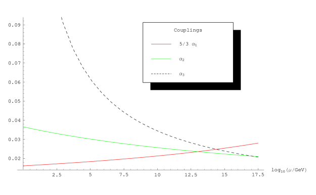
Figure 1. The running of the three couplings.

5.2. The Higgs scattering parameter and the Higgs mass

When written in terms of ${\bf H}$, and using (4.10), the quartic term

$$\frac{f_{0}}{2\,\pi^{2}}\int\,b\,|\varphi|^{4}\,\sqrt{g}\,d^{4}x=\frac{\pi^{2}}{2\,f_{0}}\frac{b}{a^{2}}\,\int\,|{\bf H}|^{4}\,\sqrt{g}\,d^{4}x$$

gives a further relation in our theory between the $\tilde{\lambda}|{\bf H}|^{4}$ coupling and the gauge couplings to be imposed at the scale $\Lambda$. This is of the form

(5.6) $$\tilde{\lambda}(\Lambda)=\,g_{3}^{2}\,\frac{b}{a^{2}}.$$

We introduce the following notation. For $v=\frac{2M}{g}$ we define the elements $(y^{\sigma}_{\cdot})$ with $\sigma=1,2,3$ the generation index and $\cdot=u,d,\nu,e$ by the relation

(5.7) $$\frac{v}{\sqrt{2}}(y^{\sigma}_{\cdot})=(m^{\sigma}_{\cdot}),$$

where the $(m^{\sigma}_{\cdot})$ are defined as in (4.15). In particular, $y^{\sigma}_{u}$ for $\sigma=3$ gives the top quark Yukawa coupling. We also set

(5.8) $$t=\log(\frac{\Lambda}{M_{Z}})\ \ \ \text{ and }\ \ \ \mu=M_{Z}e^{t}.$$

We consider the Yukawa couplings $(y^{\sigma}_{\cdot})$ as depending on the energy scale through their renormalization group equation (cf. [1], [6], [41]). We consider in particular the top quark case $y^{\sigma}_{u}(t)$ for $\sigma=3$. The running of the top quark Yukawa coupling $y_{t}=y^{\sigma}_{u}(t)$, with $\sigma=3$, is governed by the equation (cf. [45] equation (2.143) and equation (A9) of [1])

(5.9) $$\frac{dy_{t}}{dt}=\frac{1}{16\pi^{2}}\left[\frac{9}{2}y_{t}^{3}-\left(a\,g_{1}^{2}+b\,g_{2}^{2}+c\,g_{3}^{2}\right)y_{t}\right]\,,\quad(a,b,c)=(\frac{17}{12},\frac{9}{4},8)$$

The relation (5.6) could be simplified if we assume that the top quark Yukawa coupling is much larger than all the other Yukawa couplings. In this case equation (5.6) simplifies. In fact, one gets $a\sim 3\,m_{top}^{2}$ and $b\sim 3\,m_{top}^{4}$, where $m_{top}=m^{\sigma}_{u}$, with $\sigma=3$ in the notation of (4.15), so that

(5.10) $$\tilde{\lambda}(\Lambda)\sim\frac{4}{3}\,\pi\,\alpha_{3}(\Lambda)\,.$$

This agrees with [7] equation (3.31). In fact, the normalization of the Higgs field there is as in the l.h.s. of (5.23) which gives $\lambda(\mu)=4\tilde{\lambda}(\mu)$, with $\mu$ as in (5.8). In terms of the Higgs scattering parameter $\alpha_{h}$ of the standard model, (5.10) reads

(5.11) $$\alpha_{h}(\Lambda)\sim\frac{8}{3}\,$$

which agrees with [32] equation (1). Therefore, the value of $\lambda=4\,\tilde{\lambda}$ at the unification scale of $\Lambda=10^{17}$ GeV is $\lambda_{0}\sim 0.356$ showing that one does not go outside the perturbation domain.

Equation (5.10) can be used, together with the RG equations for $\lambda$ and $y^{\sigma}_{u}(t)$, with $\sigma=3$, to determine the Higgs mass at the low-energy scale $M_{Z}$.

For simplicity of notation, in the following we write

(5.12) $$y_{t}=y^{\sigma}_{u}(t),\ \ \ \text{ with }\ \ \sigma=3.$$

We have (cf. [45] equations (2.141), (2.142), (4.2) and the formula (A15) of [1]) the equation

(5.13) $$\frac{d\lambda}{dt}=\lambda\gamma+\frac{1}{8\pi^{2}}(12\lambda^{2}+B)$$

where

(5.14) $$\gamma = \,\frac{1}{16\pi^{2}}(12\,y_{t}^{2}-9\,g_{2}^{2}-3\,g_{1}^{2})$$

$$B = \,\frac{3}{16}(3\,g_{2}^{4}+2g_{1}^{2}\,g_{2}^{2}+g_{1}^{4})-3\,y_{t}^{4}\,.$$

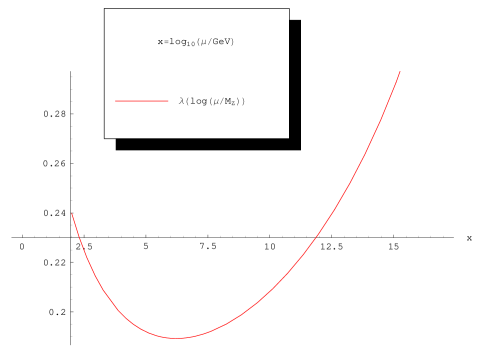
Figure 2. The running of the quartic Higgs coupling.

The Higgs mass is then given by

(5.15) $$m_{H}^{2}=\,8\lambda\,\frac{M^{2}}{g^{2}}\,,\quad m_{H}=\sqrt{2\lambda}\,\frac{2M}{g}$$

The numerical solution to these equations with the boundary value $\lambda_{0}=0.356$ at $\Lambda=10^{17}$ GeV gives $\lambda(M_{Z})\sim 0.241$ and a Higgs mass of the order of $170$ GeV. We refer to [5] and to [32] for the analysis of variants of the model.

Remark 5.1.

The estimate of equation (5.10) is obtained under the assumption that the Yukawa coupling for the top quark is the dominant term and the others are negligible. However, due to the see-saw mechanism discussed in §5.3 below, one should expect that the Yukawa coupling for the tau neutrino is also large and of the same order as the one for the top quark. Thus, the factor of $4/3$ in (5.10) should be corrected to $1$ as in (5.29) below. One can check by direct calculation that this does not affect substantially the estimate we obtain for the Higgs mass which is then around $168$ GeV.

5.3. Neutrino mixing and the see-saw mechanism

Let us briefly explain how the see-saw mechanism appears in our context. Let $D=D(Y)$ be as in (2.31). The restriction of $D(Y)$ to the subspace of ${\mathcal{H}}_{F}$ with basis the $(\nu_{R},\nu_{L},\bar{\nu}_{R},\bar{\nu}_{L})$ is given by a matrix of the form

(5.16) $$\left[\begin{array}[]{cccc}0&M_{\nu}^{*}&M_{R}^{*}&0\\ M_{\nu}&0&0&0\\ M_{R}&0&0&\bar{M}_{\nu}^{*}\\ 0&0&\bar{M}_{\nu}&0\\ \end{array}\right]$$

where $M_{\nu}=\frac{2M}{g}K_{\nu}$ with $K_{\nu}$ as in (4.39).

The largest eigenvalue of $M_{R}$ is set to the order of the unification scale by the equations of motion of the spectral action as in the following result.

Lemma 5.2.

Assume that the matrix $M_{R}$ is a multiple of a fixed matrix $k_{R}$, i.e. is of the form $M_{R}=x\,k_{R}$. In flat space, and assuming that the Higgs vacuum expectation value is negligible with respect to unification scale, the equations of motion of the spectral action fix $x$ to be either $x=0$ (unstable) or satisfying

(5.17) $$x^{2}=\frac{2\,f_{2}\,\Lambda^{2}\,{\rm Tr}(k_{R}^{*}k_{R})}{f_{0}\,{\rm Tr}((k_{R}^{*}k_{R})^{2})}.$$

Proof.

The value of $x$ is fixed by the equations of motion of the spectral action

(5.18) $$\partial_{u}{\rm Tr}(f(D_{A}/\Lambda))=0,$$

with $u=x^{2}$.

One can see from (3.16) that $x$ only appears in the coefficients $c$, $d$, and $e$. In the variation (5.18), the terms in the spectral action (3.13) of Theorem 3.13 containing the coefficient $c$ and $e$ produce linear terms in $x^{2}$, proportional to the scalar curvature $R$ and the square $|\varphi|^{2}$ of the Higgs vacuum expectation value, and an additional linear term coming from the cosmological term. The cosmological term also contains the coefficient $d$, which depends quadratically on $x^{2}$. In flat space, and under the assumption that $|\varphi|^{2}$ is sufficiently small, (5.18) then corresponds to minimizing the cosmological term.

This gives

(5.19) $$\partial_{x}(-f_{2}\,\Lambda^{2}\,c+\frac{f_{0}}{4}\,d)=0,\ \ \ \ c=x^{2}\,{\rm Tr}(k_{R}^{*}k_{R}),\ \ \ \ d=x^{4}\,{\rm Tr}((k_{R}^{*}k_{R})^{2}).$$

Thus, we get $M_{R}=xk_{R}$ with $x$ satisfying (5.17). In other words we see that

(5.20) $$M_{R}^{*}M_{R}=\frac{2\,f_{2}\,\Lambda^{2}}{f_{0}}\,\frac{k_{R}^{*}k_{R}\,{\rm Tr}(k_{R}^{*}k_{R})}{{\rm Tr}((k_{R}^{*}k_{R})^{2})}$$

∎

The Dirac mass $M_{\nu}$ is of the order of the Fermi energy $v$ and hence much smaller. The eigenvalues of the matrix (5.16) are then given, simplifying to one generation, by

(5.21) $$\frac{1}{2}\,(\pm m_{R}\,\pm\sqrt{m_{R}^{2}+4\,v^{2}}),$$

where $m_{R}$ denotes the eigenvalues of $M_{R}$, which is of the order of $\Lambda$ by the result of Lemma 5.2, see (5.20).

This gives two eigenvalues very close to $\pm m_{R}$ and two others very close to $\pm\frac{v^{2}}{m_{R}}$ as can be checked directly from the determinant of the matrix (5.16), which is equal to $|M_{\nu}|^{4}\sim v^{4}$ (for one generation).

Remark 5.3.

This is compatible with the scenario proposed by Fukigita and Yanagida (cf. [37]) following the ideas of Sakharov and t’Hooft, to explain the asymmetry between matter and antimatter in the universe.

Typical estimates for the large masses of the right handed neutrinos i.e. the eigenvalues of $M_{R}$ are given (cf. [37]) by

(5.22) $$(m_{R})_{1}\geq 10^{7}GeV\,,\quad(m_{R})_{2}\geq 10^{12}GeV\,,\quad(m_{R})_{3}\geq 10^{16}GeV\,.$$

5.4. The fermion–boson mass relation

There are two different normalizations for the Higgs field in the literature.

1. In Veltman [46] the kinetic term has a factor of $\frac{1}{2}$

2. In Mohapatra–Pal it has a factor of $1$ (cf. [37] equation (1.43))

One passes from one to the other by

(5.23) $$\varphi_{mp}=\frac{1}{\sqrt{2}}\,\varphi_{velt}$$

In [7] we used the second convention. Let us then stick to that for the definition of the Yukawa couplings $(y^{\sigma}_{\cdot})(t)$ which is then given by (5.7) above.

The mass of the top quark is governed by the top quark Yukawa coupling $y_{t}=y^{\sigma}_{u}(t)$ with $\sigma=3$ by the equation

(5.24) $$m_{top}(t)=\frac{1}{\sqrt{2}}\frac{2M}{g}\,y_{t}=\frac{1}{\sqrt{2}}\,v\,y_{t},$$

where $v=\frac{2M}{g}$ is the vacuum expectation value of the Higgs field. The running of the top quark Yukawa coupling $y_{t}=y^{\sigma}_{u}(t)$, with $\sigma=3$, is governed by equation (5.9).

In terms of the Yukawa couplings $(y^{\sigma}_{\cdot})$ of (5.7), the mass constraint (4.16) reads as

(5.25) $$\frac{v^{2}}{2}\sum_{\sigma}\,(y^{\sigma}_{\nu})^{2}+(y^{\sigma}_{e})^{2}+3\,(y^{\sigma}_{u})^{2}+3\,(y^{\sigma}_{d})^{2}=\,2\,g^{2}\,v^{2},$$

with $v=\frac{2M}{g}$ the vacuum expectation value of the Higgs, as above.

In the traditional notation for the Standard Model the combination

$$Y_{2}=\sum_{\sigma}\,(y^{\sigma}_{\nu})^{2}+(y^{\sigma}_{e})^{2}+3\,(y^{\sigma}_{u})^{2}+3\,(y^{\sigma}_{d})^{2}$$

is denoted by $Y_{2}=Y_{2}(S)$ (cf. [1]). Thus, the mass constraint (4.16) is of the form

(5.26) $$Y_{2}(S)=4\,g^{2}.$$

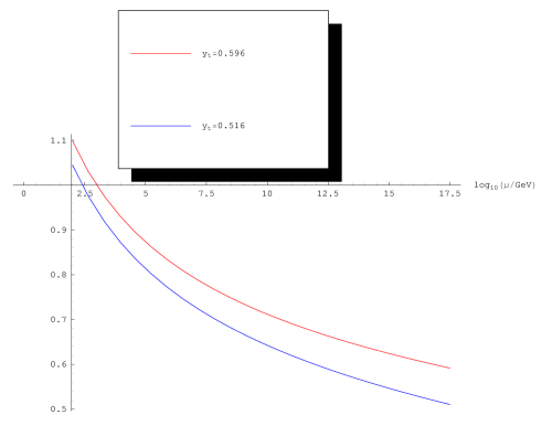
Figure 3. The running of the top quark Yukawa coupling.

Assuming that it holds at a unification scale of $10^{17}$ GeV and neglecting all other Yukawa couplings with respect to the top quark $y^{\sigma}_{u}$, with $\sigma=3$, we get the following approximate form of (4.16),

(5.27) $$y^{\sigma}_{u}=\frac{2}{\sqrt{3}}\,g,\ \ \ \text{ with }\ \sigma=3.$$

The value of $g$ at a unification scale of $10^{17}$ GeV is $\sim 0.517$. Thus, neglecting the $\tau$ neutrino Yukawa coupling, we get the simplified relation

(5.28) $$y_{t}=\,\frac{2}{\sqrt{3}}\,g\sim 0.597\,,\quad t\sim 34.6\,.$$

Thus, in first approximation, numerical integration of the differential equation (5.9) with the boundary condition (5.28) gives the value $y_{0}=\sim 1.102$ and a top quark mass of the order of $\frac{1}{\sqrt{2}}y_{0}\,v\sim\,173.683\,y_{0}$ GeV.

The see-saw mechanism, however, suggests that the Yukawa coupling for the $\tau$ neutrino is of the same order as the top quark Yukawa coupling. Indeed, even if the tau neutrino mass has an upper bound of the order of (cf. [37])

$$m_{\nu_{\tau}}\leq 18.2\ \text{MeV},$$

the see-saw mechanism allows for a large Yukawa coupling term by the relation (5.21) and (5.22). It is then natural to take the Yukawa coupling $y^{\sigma}_{\nu}$, with $\sigma=3$ for the tau neutrino to be the same, at unification, as that of the top quark. This introduces in (5.28) a correction factor of $\sqrt{\frac{3}{4}}$. In fact, for $x_{t}=y^{\sigma}_{\nu}(t)$ and $y_{t}=y^{\sigma}_{u}(t)$, with $\sigma=3$, we now have

(5.29) $$Y_{2}(S)\sim x_{t}^{2}+3y_{t}^{2}\sim\frac{4}{3}\cdot 3y_{t}^{2}=4\,y_{t}^{2}\Rightarrow y_{t}\sim g$$

This has the effect of lowering the value of $y_{0}$ to $y_{0}\sim 1.04$, which yields an acceptable value for the top quark mass, given that we neglected all other Yukawa couplings except for the top and the tau neutrino.

5.5. The gravitational terms

We now discuss the behavior of the gravitational terms in the spectral action, namely

(5.30) $$\int\biggl{(}\frac{1}{2\kappa_{0}^{2}}\,R+\alpha_{0}\,C_{\mu\nu\rho\sigma}\,C^{\mu\nu\rho\sigma}+\gamma_{0}+\tau_{0}\,R^{*}R^{*}-\xi_{0}\,R\,|{\bf H}|^{2}\biggl{)}\sqrt{g}\,d^{4}x.$$

The traditional form of the Euclidean higher derivative terms that are quadratic in curvature is (see e.g. [21], [12])

(5.31) $$\int\ \,\biggl{(}\frac{1}{2\eta}\,C_{\mu\nu\rho\sigma}\,C^{\mu\nu\rho\sigma}-\frac{\omega}{3\eta}\,R^{2}+\frac{\theta}{\eta}\,E\,\biggr{)}\,\sqrt{g}\,d^{4}x,$$

with $E=R^{*}R^{*}$ the topological term which is the integrand in the Euler characteristic

(5.32) $$\chi(M)=\ \frac{1}{32\pi^{2}}\int\ E\,\sqrt{g}\,d^{4}x=\frac{1}{32\pi^{2}}\int\ \,R^{*}R^{*}\sqrt{g}\,d^{4}x$$

The running of the coefficients of the Euclidean higher derivative terms in (5.31), determined by the renormalization group equation, is gauge independent and is given by (see e.g. [3] equations 4.49 and 4.71 and [21], [12])

$$\beta_{\eta} =-\frac{1}{\left(4\pi\right)^{2}}\frac{133}{10}\eta^{2}$$

$$\beta_{\omega} =-\frac{1}{\left(4\pi\right)^{2}}\frac{25+1098\,\omega+200\,\omega^{2}}{60}\eta$$

$$\beta_{\theta} =\frac{1}{\left(4\pi\right)^{2}}\frac{7\left(56-171\,\theta\right)}{90}\eta$$

while the graphs are shown in Figures 4, 5, 6. Notice that the infrared behavior of these terms approaches the fixed point $\eta=0$, $\omega=-0.0228$, $\theta=0.327$. The coefficient $\eta$ goes to zero in the infrared limit, sufficiently slowly, so that, up to scales of the order of the size of the universe, its inverse remains $O(1)$. On the other hand, $\eta(t)$, $\omega(t)$ and $\theta(t)$ have a common singularity at an energy scale of the order of $10^{23}$ GeV, which is above the Planck scale. Moreover, within the energy scales that are of interest to our model $\eta(t)$ is neither too small nor too large (it does not vary by more than a single order of magnitude between the Planck scale and infrared energies).

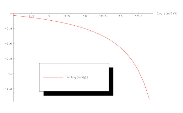
Figure 4. The running of the Weyl curvature term in (5.31).

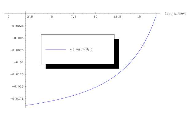
Figure 5. The running of the ratio of the coefficients of the $R^{2}$ term and the Weyl term in (5.31).

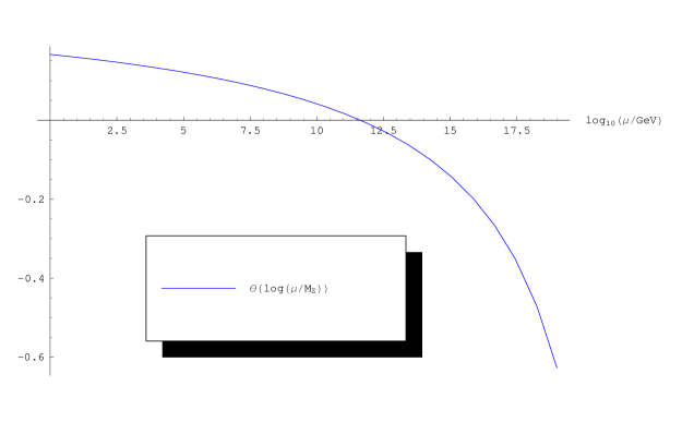
Figure 6. The running of the ratio of the coefficients of the topological term and the Weyl term in (5.31).

The only known experimental constraints on the values of the coefficients of the quadratic curvature terms $R_{\mu\nu}R^{\mu\nu}$ and $R^{2}$ at low energy are very weak and predict that their value should not exceed $10^{74}$ (cf. e.g. [21]). In our case, this is guaranteed by the running described above. Note that we have neglected the coupling $R\,{\bf H}^{2}$ with the Higgs field which ought to be taken into account in a finer analysis.

The coefficient of the Einstein term is of the form

(5.33) $$\frac{1}{\kappa_{0}^{2}}=\ \frac{96\,f_{2}\,\Lambda^{2}-f_{0}\,c}{12\pi^{2}}.$$

With the above notation, by the result of Lemma 5.2, we get

$$c=\,x^{2}\,{\rm Tr}(k_{R}^{*}k_{R})=\frac{2\,f_{2}\,\Lambda^{2}\,({\rm Tr}(k_{R}^{*}k_{R}))^{2}}{f_{0}\,{\rm Tr}((k_{R}^{*}k_{R})^{2})}.$$

Thus, the range of variation of $\frac{({\rm Tr}(k_{R}^{*}k_{R}))^{2}}{{\rm Tr}((k_{R}^{*}k_{R})^{2})}$ for $N$ generations is the interval $[1,N]$. In particular, with $N=3$ we get

(5.34) $$\frac{90\,f_{2}\,\Lambda^{2}}{12\pi^{2}}\leq\frac{1}{\kappa_{0}^{2}}\leq\frac{94\,f_{2}\,\Lambda^{2}}{12\pi^{2}}$$

This estimate is not modified substantially if one takes into account the contribution from the $R\,{\bf H}^{2}$ term using the vacuum expectation value of the Higgs field. Thus we see that independently of the choice of $k_{R}$ the coefficient $\kappa_{0}^{-2}$ of the Einstein term $\frac{1}{2}\,\int\,R\,\sqrt{g}\,d^{4}x$ is positive and of the order of $f_{2}\,\Lambda^{2}$. Thus the result is similar to what happened for the Einstein-Yang-Mills system [8] and the sign is the correct one. As far as the size is concerned let us now compare the value we get for $\kappa_{0}$ with the value given by Newton’s constant. In our case we get

$$\kappa_{0}^{-1}\sim\Lambda\,\sqrt{f}_{2}$$

Thus if we take for $\Lambda$ the energy scale of the meeting point of the electroweak and strong couplings, namely $\Lambda\sim 1.1\times 10^{17}$ GeV, we get

$$\kappa_{0}^{-1}\sim 1.1\times 10^{17}\,\sqrt{f}_{2}\,{\rm GeV}$$

On the other hand using the usual form of the gravitational action

(5.35) $$S(g)=\frac{1}{16\pi G}\,\int_{M}R\,dv\,,$$

and the experimental value of Newton’s constant at ordinary scales one gets the coupling constant

$$\kappa_{0}(M_{Z})=\,\sqrt{8\pi G}\,,\quad\kappa_{0}^{-1}\sim 1.221\,10^{19}/\sqrt{8\pi}\sim 2.43\times 10^{18}\,{\rm GeV}.$$

One should expect that the Newton constant runs at higher energies (cf. e.g. [21], [40], [39]) and increases at high energy when one approaches the Planck scale. Thus the ratio

(5.36) $$\rho=\kappa_{0}(\Lambda)/\kappa_{0}(M_{Z})$$

for $\Lambda\sim 1.1\times 10^{17}$ GeV, which measures the running at unification scale, should be larger than $1$.

By the normalization of the kinetic terms of the gauge fields, one has (4.10)

$$f_{0}=\,\frac{\pi^{2}}{2\,g^{2}}=\,\frac{\pi}{8\,\alpha_{2}(\Lambda)}\sim 18.45\,.$$

Thus

$$1.1\times 10^{17}\,\sqrt{f}_{0}\sim 4.726\times 10^{17}$$

It follows that if

(5.37) $$f_{2}/f_{0}=\tau^{2}/\rho^{2}\,,\ \ \tau\sim 5.1$$

one obtains the correct physical value for the Newton constant. In fact starting with a test function $g$ such that $g_{2}=g_{0}$, equality (5.37) holds provided one performs the transformation

$$g\mapsto f\,,\quad f(x)=g(\frac{\rho\,x}{\tau})\,.$$

5.6. The cosmological term

The cosmological term depends, in our model, on the remaining parameter $f_{4}$.

Lemma 5.4.

Under the hypothesis of Lemma 5.2, the cosmological term gives

(5.38) $$\frac{1}{\pi^{2}}\left(48f_{4}-\frac{{\rm Tr}(k_{R}^{*}k_{R})^{2}}{{\rm Tr}((k_{R}^{*}k_{R})^{2})}\frac{f_{2}^{2}}{f_{0}}\right)\Lambda^{4}.$$

Proof.

In (3.45) we have the cosmological term

$$\frac{1}{\pi^{2}}\left(48f_{4}\Lambda^{4}-f_{2}c\Lambda^{2}+\frac{f_{0}}{4}d\right),$$

where the coefficients $c$ and $d$ are given by

$$c={\rm Tr}(Y_{R}^{*}Y_{R})\ \ \ \text{ and }\ \ \ d={\rm Tr}((Y_{R}^{*}Y_{R})^{2})).$$

We use the result of Lemma 5.2 and (5.20). We obtain

$$c=\frac{2\,f_{2}\,\Lambda^{2}}{f_{0}}\frac{{\rm Tr}(k_{R}^{*}k_{R})^{2}}{{\rm Tr}((k_{R}^{*}k_{R})^{2})}\ \ \ \text{ and }d=\frac{4f_{2}^{2}\Lambda^{4}}{f_{0}^{2}}\frac{{\rm Tr}(k_{R}^{*}k_{R})^{2}}{{\rm Tr}((k_{R}^{*}k_{R})^{2})}.$$

∎

The positivity of the $f_{j}$, and the freedom in choosing the $f_{4}$ makes it possible to adjust the value of the cosmological term. Notice that, if one assumes that the function $f$ is decreasing (and positive as usual), then the Schwartz inequality gives the constraint

$$f_{2}^{2}\leq f_{0}f_{4}.$$

The Schwartz inequality also gives the estimate

$$\frac{{\rm Tr}(k_{R}^{*}k_{R})^{2}}{{\rm Tr}((k_{R}^{*}k_{R})^{2})}\leq 3$$

in (5.38). Thus, for a decreasing positive function, this cosmological term is positive. Of course to obtain the physical cosmological constant one needs to add to this term the contribution from the vacuum expectation value of the various fields which give an additional contribution of the order of $(96-28)\frac{1}{32\pi^{2}}\Lambda^{4}$ and generate a fine tuning problem to ensure that the value of the cosmological constant at ordinary scale is small. It is natural in this context to replace the cut-off $\Lambda$ by a dynamical dilaton field as in [9], cf. §5.7.3 below.

5.7. The tadpole term and the naturalness problem

The naturalness problem for the standard model arises from the quadratically divergent corrections to the tadpole term

(5.39) $$\delta\beta_{h}\sim\Lambda^{2}\,\sum\,c_{n}\,\log(\Lambda/M_{Z})^{n}$$

that are required in order to maintain the Higgs vacuum expectation value at the electroweak scale (cf. [43] §II.C.4). In our set-up the only natural scale is the unification scale. Thus, an explanation for the weak scale still remains to be found. We shall not attempt to address this problem here but make a few remarks.

5.7.1. Naturalness and fine tuning

When the cutoff regularization method is used a number of diagrams involving the Higgs fields are actually quadratically divergent and thus generate huge contributions to the tadpole bare term. To be more specific, one has the following quadratically divergent diagrams:

• Minimal coupling with $W$ and $B$ fields

• Quartic self-coupling of Higgs fields

• Yukawa couplings with fermions

If we want to fix the Higgs vacuum at $\frac{2M}{g}$ in the standard model we need to absorb the huge quadratic term in $\Lambda$ in the tadpole term of the action. The tadpole constant $\beta_{h}$ then acquires a quadratically divergent contribution

(5.40) $$\frac{1}{2}\delta\beta_{h}\sim\frac{\Lambda^{2}}{32\pi^{2}}\,q(t)\,,\ t=\log(\Lambda/M_{Z})\,,$$

where (cf. [22], [31], [43])

(5.41) $$q(t)=\,\frac{9}{4}\,g_{2}^{2}+\frac{3}{4}\,g_{1}^{2}+6\lambda-6\,y_{t}^{2}\,,$$

where, as above, $y_{t}=y^{\sigma}_{u}(t)$, with $\sigma=3$ is the top quark Yukawa coupling. This form of (5.41) holds under the assumption that the contribution coming from the top quark is the dominant term in the Yukawa coupling (see, however, the previous discussion on the term $y^{\sigma}_{\nu}(t)$ with $\sigma=3$ in §5.4).

One can check that the contribution $y_{t}$ is sufficiently large in the standard model so that, for small $t$, $q(t)$ is negative. However, as shown in Figure 7 the expression $q(t)$ changes sign at energies of the order of $10^{10}$ GeV, and is then positive, with a value at unification $\sim 1.61$.

While the plot 7 uses the known experimental values, one can show directly that our boundary conditions at unification scale $t_{unif}$ also imply that $q(t_{unif})>0$. In fact it is better to replace $3y_{t}^{2}$ by $Y_{2}$ and we can then use our mass relation at unification in the form (5.26)

$$Y_{2}=4\,g^{2}$$

Also at unification we have a precise form of $\lambda$ namely (5.6), together with $\lambda=4\tilde{\lambda}$ and get

$$\lambda=\,4\,g^{2}\,\frac{b}{a^{2}}$$

We can thus rewrite (5.41) as (with $g=g_{2}$)

(5.42) $$q(t_{unif})=\,\frac{9}{4}\,g^{2}+\frac{3}{4}\,g_{1}^{2}+24\,g^{2}\,\frac{b}{a^{2}}-8\,g^{2}\,,$$

We can now use the inequality

$$\frac{b}{a^{2}}\geq\frac{1}{4}$$

which holds even with a large tau neutrino Yukawa coupling, to get

(5.43) $$q(t_{unif})\geq\,\frac{9}{4}\,g^{2}+\frac{3}{4}\,g_{1}^{2}+24\,g^{2}\,\frac{1}{4}-8\,g^{2}=\frac{1}{4}\,g^{2}+\frac{3}{4}\,g_{1}^{2}>0\,.$$

5.7.2. Sign of the quadratic term

In the spectral action we also have a similar term which is quadratic in $\Lambda$ namely the term $-\mu_{0}^{2}\,{\bf H}^{2}$ of (4.11) where $\mu_{0}^{2}=2\frac{f_{2}\,\Lambda^{2}}{f_{0}}-\frac{e}{a}$. We show that, under the simplifying hypothesis of Lemma 5.2, the coefficient of $\Lambda^{2}$ in $\mu_{0}^{2}$ in the spectral action is generally positive but can be small and have an arbitrary sign provided there are at least two generations and one chooses suitable Yukawa and Majorana mass matrices. The reason why we can use Lemma 5.2 is that we are interested in small values of $\mu_{0}^{2}$, a more refined analysis would be required to take care of the general case. By Lemma 5.2 we have $M_{R}=xk_{R}$ with $x$ as in (5.17).

Lemma 5.5.

Under the hypothesis of Lemma 5.2, the coefficient of the Higgs quadratic term $-\mu_{0}^{2}\,{\bf H}^{2}$ in the spectral action is given by

(5.44) $$\mu_{0}^{2}=\,2\,\Lambda^{2}\,\frac{f_{2}}{f_{0}}\,(1-X)=\,(1-X)\,\frac{4\,g^{2}\,\Lambda^{2}}{\pi^{2}}\,f_{2}$$

where

(5.45) $$X=\frac{{\rm Tr}(k_{R}^{*}k_{R}\,k_{\nu}^{*}k_{\nu})\,{\rm Tr}(k_{R}^{*}k_{R})}{{\rm Tr}(k_{\nu}^{*}k_{\nu}+k_{e}^{*}k_{e}+3(k_{u}^{*}k_{u}+k_{d}^{*}k_{d})){\rm Tr}((k_{R}^{*}k_{R})^{2})}$$

Proof.

One has $\mu_{0}^{2}=\ 2\,\frac{f_{2}\,\Lambda^{2}}{f_{0}}-\frac{e}{a}$ with $e$ and $a$ as in (3.16).

Using (5.20) and (4.13) we then get the first equality in (5.44). The second follows from (4.10). ∎

In order to compare $X$ with $1$ we need to determine the range of variation of the largest eigenvalue of $\frac{k_{R}^{*}k_{R}\,{\rm Tr}(k_{R}^{*}k_{R})}{{\rm Tr}((k_{R}^{*}k_{R})^{2})}$ as a function of the number of generations.

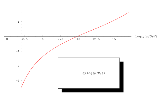
Figure 7. The running of the tadpole term.

Lemma 5.6.

The range of variation of the largest eigenvalue,

$$\rho(k_{R})=\,||\frac{k_{R}^{*}k_{R}\,{\rm Tr}(k_{R}^{*}k_{R})}{{\rm Tr}((k_{R}^{*}k_{R})^{2})}||$$

for $k_{R}\in M_{N}({\mathbb{C}})$, is the interval

$$[1,\frac{1}{2}(1+\sqrt{N})]$$

Proof.

Notice first that one has

$${\rm Tr}((k_{R}^{*}k_{R})^{2})\leq{\rm Tr}(k_{R}^{*}k_{R})\,||k_{R}^{*}k_{R}||$$

so that the inequality $\geq 1$ follows. Moreover this lower bound is reached exactly when $k_{R}^{*}k_{R}$ is a multiple of an idempotent which means that $k_{R}$ is a multiple of a partial isometry. To understand the upper bound, we can assume that $k_{R}^{*}k_{R}$ is diagonal with eigenvalues $\lambda_{j}^{2}$. We just need to understand the range of variation of $F_{N}(\lambda)=\frac{\lambda_{1}^{2}\,\sum\,\lambda_{j}^{2}}{\sum\,\lambda_{j}^{4}}$. Using Lagrange multipliers one gets that, at an extremum, all the $\lambda_{j}^{2}$ for $j\neq 1$ are equal. Thus, one just needs to get the range of variation of the simpler function $f_{N}(u)=\frac{u^{2}(u^{2}+N-1)}{u^{4}+N-1}$. Computing the value of $f_{N}$ at the maximum $u^{2}=1+\sqrt{N}$ yields the required answer. ∎

We thus see that the maximal value for $X$ obtained by replacing $k_{R}^{*}k_{R}$ by its maximal eigenvalue, yields the inequality

(5.46) $$X\leq\,\frac{(1+\sqrt{N})}{2}\,\frac{{\rm Tr}(k_{\nu}^{*}k_{\nu})}{{\rm Tr}(k_{\nu}^{*}k_{\nu}+k_{e}^{*}k_{e}+3(k_{u}^{*}k_{u}+k_{d}^{*}k_{d}))}$$

As we show now the range of variation of the simplified quadratic term (i.e. the right hand side of equation (5.44)) depends on the number $N$ of generations.

Proposition 5.7.

Let $N$ be the number of generations.

1. If $N=1$, or if $k_{R}$ is a scalar multiple of a partial isometry, the quadratic term (5.44) is positive and its size of the order of $\frac{f_{2}\,\Lambda^{2}}{f_{0}}$.

2. If $N\geq 2$, the quadratic term (5.44) can vanish and have arbitrary sign, provided one chooses $k_{R}$, $k_{\nu}$ appropriately.

Proof.

1) By lemma 5.6 we have $\rho(k_{R})=1$ and thus by (5.45),

$$X\leq\frac{{\rm Tr}(k_{\nu}^{*}k_{\nu})}{{\rm Tr}(k_{\nu}^{*}k_{\nu}+k_{e}^{*}k_{e}+3(k_{u}^{*}k_{u}+k_{d}^{*}k_{d}))}<1$$

Thus

$$\mu_{0}^{2}=\,2\,\Lambda^{2}\,\frac{f_{2}}{f_{0}}\,(1-X)$$

is positive and of the same order as $\frac{f_{2}\,\Lambda^{2}}{f_{0}}$.

2) We take $N=3$ and explain how to choose $k_{R}$, $k_{\nu}$ etc… so that the coefficient of the quadratic term vanishes. We choose $k_{R}$ such that the eigenvalues of $k_{R}^{*}k_{R}$ are of the form $(1+\sqrt{3},1,1)$. Then as in lemma 5.6 the eigenvalues of $\frac{k_{R}^{*}k_{R}\,{\rm Tr}(k_{R}^{*}k_{R})}{{\rm Tr}((k_{R}^{*}k_{R})^{2})}$ are $\frac{1}{2}(1+\sqrt{3},1,1)$. We can now choose $k_{\nu}$ in such a way that it is is diagonal in the same basis as $k_{R}^{*}k_{R}$ with a single order one eigenvalue on the first basis vector while the two other eigenvalues are small. It follows that

$$X\sim\frac{1}{2}(1+\sqrt{3})\frac{{\rm Tr}(k_{\nu}^{*}k_{\nu})}{{\rm Tr}(k_{\nu}^{*}k_{\nu}+k_{e}^{*}k_{e}+3(k_{u}^{*}k_{u}+k_{d}^{*}k_{d}))}\sim 1$$

provided that

$$\frac{1}{2}(\sqrt{3}-1)\,{\rm Tr}(k_{\nu}^{*}k_{\nu})\sim{\rm Tr}(k_{e}^{*}k_{e}+3(k_{u}^{*}k_{u}+k_{d}^{*}k_{d}))$$

∎

Neglecting the Yukawa couplings except for the tau neutrino and the top quark, one gets $k_{\nu_{\tau}}\sim 2.86\,k_{top}$. While the seesaw mechanism allows for a large Yukawa matrix for the neutrinos, the above relation yields a Yukawa coupling for the tau neutrino which is quite a bit larger than the expected one as in GUT theories where it is similar to the top Yukawa coupling. In summary we have shown that $\mu_{0}^{2}>0$ except under the above special choice of Yukawa coupling matrices. We have been working under the simplifying hypothesis of Lemma 5.2 and to eliminate that, a finer analysis involving the symmetry breaking of the potential in the variables $x$ and $\varphi$ (after promoting $x$ to a scalar field) would be necessary.

5.7.3. The dilaton field

In fact there is another scalar field which plays a natural role in the above set-up and which has been neglected for simplicity in the above discussion. Indeed as in [9] it is natural when considering the spectral action (in particular on non-compact spaces) to replace the cut-off $\Lambda$ by a dynamical dilaton field. We refer to [9] for the computation of the spectral action with dilaton and its comparison with the Randall-Sundrum model. Its extension to the present set-up is straightforward using the technique of [9]. One obtains a model which is closely related to the model of scale invariant extended inflation of [28].

5.7.4. Geometric interpretation

Our geometric interpretation of the standard model gives a picture of space-time as the product of an ordinary spin manifold (in Euclidean signature) by a finite noncommutative geometry F. The geometry of $F$ is specified by its Dirac operator $D_{F}$ whose size is governed by the vacuum expectation value of the Higgs field. In other words it is the (inverse of the) size of the space $F$ that specifies the electroweak scale. It is thus tempting to look for an explanation for the smallness of the ratio $M_{Z}/M_{P}$ along the same lines as inflation as an explanation for the large size of the observable universe in Planck units.

6. Appendix: Gilkey’s Theorem

The square of the Dirac operator appearing in the spectral triple of a noncommutative space is written in a form suitable to apply the standard local formulas for the heat expansion (see [26] §4.8). We now briefly recall the statement of Gilkey’s Theorem ([26] Theorem 4.8.16). One starts with a compact Riemannian manifold $M$ of dimension $m$, with metric $g$ and one lets $F$ be a vector bundle on $M$ and $P$ a differential operator acting on sections of $F$ and with leading symbol given by the metric tensor. Thus locally one has,

(6.1) $$P=-\left(g^{\mu\nu}I\,\partial_{\mu}\partial_{\nu}+A^{\mu}\partial_{\mu}+B\right),$$

where $g^{\mu\nu}$ plays the role of the inverse metric, $I$ is the unit matrix, $A^{\mu}$ and $B$ are endomorphisms of the bundle $F$. The Seeley-De witt coefficients are the terms $a_{n}(x,P)$ in the heat expansion, which is of the form

(6.2) $${\rm Tr}\,e^{-tP}\sim\sum_{n\geq 0}t^{\frac{n-m}{2}}\int_{M}\,a_{n}(x,P)\,dv(x)$$

where $m$ is the dimension of the manifold and $dv(x)=\sqrt{\det\,g_{\mu\nu}}\,d^{m}\,x$ where $g_{\mu\nu}$ is the metric on $M$.

By Lemma 4.8.1 of [26] the operator $P$ is uniquely written in the form

(6.3) $$P=\,\nabla^{*}\,\nabla-\,{\mathcal{E}}$$

where $\nabla$ is a connection on $F$, $\nabla^{*}\,\nabla$ the connection Laplacian and where ${\mathcal{E}}$ is an endomorphism of $F$. The explicit formulas for the connection $\nabla$ and the endomorphism ${\mathcal{E}}$ are

(6.4) $$\nabla_{\mu}=\,\partial_{\mu}\,+\,\omega^{\prime}_{\mu}$$

(6.5) $$\omega^{\prime}_{\mu}=\frac{1}{2}\,g_{\mu\nu}({A}^{\nu}+\Gamma^{\nu}\cdot{\rm id})$$

(6.6) $${\mathcal{E}}={B}-g^{\mu\nu}(\partial_{\mu}\,\omega^{\prime}_{\nu}+\omega^{\prime}_{\mu}\,\omega^{\prime}_{\nu}-\Gamma_{\mu\nu}^{\rho}\,\omega^{\prime}_{\rho})$$

Where one lets $\Gamma_{\mu\nu}^{\rho}\left(g\right)$ be the Christoffel symbols of the Levi-Civita connection of the metric $g$ and

$$\Gamma^{\rho}\left(g\right)=g^{\mu\nu}\Gamma_{\mu\nu}^{\rho}\left(g\right)$$

One lets $\Omega$ be the curvature of the connection $\nabla$ so that (cf. [26] Lemma 4.8.1),

(6.7) $$\Omega_{\mu\nu}=\partial_{\mu}\,\omega^{\prime}_{\nu}-\partial_{\nu}\,\omega^{\prime}_{\mu}+[\omega^{\prime}_{\mu},\,\omega^{\prime}_{\nu}]$$

The Seeley-de Witt coefficients $a_{n}(P)$ vanish for odd values of $n$. The first three $a_{n}$’s for $n$ even have the following explicit form in terms of the Riemann curvature tensor $R$, the curvature $\Omega$ of the connection $\nabla$ and the endomorphism ${\mathcal{E}}$,

Theorem 6.1.

[26] One has :

(6.8) $$a_{0}(x,P) = (4\pi)^{-m/2}{\rm Tr}({\rm id})$$

(6.9) $$a_{2}(x,P) = (4\pi)^{-m/2}{\rm Tr}\left(-\frac{R}{6}\,{\rm id}+{\mathcal{E}}\right)$$

$$a_{4}(x,P) = (4\pi)^{-m/2}\frac{1}{360}{\rm Tr}(-12R;_{\mu}{}^{\mu}+5R^{2}-2R_{\mu\nu}\,R^{\mu\nu}$$

$$+ 2R_{\mu\nu\rho\sigma}\,R^{\mu\nu\rho\sigma}-60\,R\,{\mathcal{E}}+180\,{\mathcal{E}}^{2}+60\,{\mathcal{E}};_{\mu}{}^{\mu}$$

$$+ 30\,\Omega_{\mu\nu}\,\Omega^{\mu\nu})$$

Remark 6.2.

Notice that ${\mathcal{E}}$ only appears through the terms

(6.11) $${\rm Tr}\left(-\frac{R}{6}\,{\rm id}+{\mathcal{E}}\right)\,,\quad{\rm Tr}\left((-\frac{R}{6}\,{\rm id}+{\mathcal{E}})^{2}\right)$$

and the boundary term ${\rm Tr}({\mathcal{E}};_{\mu}{}^{\mu})$.

Here $R;_{\mu}{}^{\mu}=\nabla_{\mu}\nabla^{\mu}R$ and similarly ${\mathcal{E}};_{\mu}{}^{\mu}=\nabla_{\mu}\nabla^{\mu}{\mathcal{E}}$.

6.1. The generalized Lichnerowicz formula

Let $M$ be a compact Riemannian spin manifold of dimension $m$, $S$ the spinor bundle with the canonical riemannian connection $\nabla_{S}$. Let $V$ be a hermitian vector bundle over $M$ with a compatible connection $\nabla_{V}$. One lets ${\partial/}_{V}$ be the Dirac operator on $S\otimes V$ endowed with the tensor product connection ([34] Proposition 5.10)

(6.12) $$\nabla(\xi\otimes v)=\,(\nabla_{S}\,\xi)\otimes v+\,\xi\otimes(\nabla_{V}\,v)$$

Let then $R_{V}$ be the bundle endomorpism of the bundle $S\otimes V$ defined by

(6.13) $$R_{V}(\xi\otimes v)=\,\frac{1}{2}\,\sum_{j,\,k=1}^{m}\,(\gamma_{j}\gamma_{k}\,\xi)\otimes(R(V)_{jk}\,v)$$

where $R(V)$ is the curvature tensor of the bundle $V$.

One then has ([34] Theorem 8.17)

Theorem 6.3.

let $s=-R$ be the scalar curvature of $M$, then the Dirac operator ${\partial/}_{V}$ satisfies

(6.14) $${\partial/}_{V}^{2}=\nabla^{*}\,\nabla+\frac{1}{4}\,s+\,R_{V}$$

where $\nabla^{*}\,\nabla$ is the connection Laplacian of $S\otimes V$.

Notice that all three terms of the right hand side of (6.14) are self-adjoint operators by construction. In particular $R_{V}$ is self-adjoint. One can write $R_{V}$ in the following form where the terms in the sum are pairwise orthogonal for the natural inner product on the Clifford algebra (induced by the Hilbert-Schmidt inner product $\langle A,B\rangle={\rm Tr}(A^{*}B)$ in the spin representation)

(6.15) $$R_{V}=\,\sum_{j<k}\,\gamma_{j}\gamma_{k}\otimes R(V)_{j\,k}$$

6.2. The asymptotic expansion and the residues

The spectral action can be expanded in decreasing powers of the scale $\Lambda$ in the form

(6.16) $$\mathrm{Trace}\,(f(D/\Lambda))\sim\,\sum_{k\in\,\Pi^{+}}\,f_{k}\,\Lambda^{k}\,{\int\!\!\!\!\!\!-}\,|D|^{-k}\,+\,f(0)\,\zeta_{D}(0)+\,o(1),$$

where the function $f$ only appears through the scalars

(6.17) $$f_{k}=\,\int_{0}^{\infty}f(v)\,v^{k-1}\,dv.$$

The term independent of the parameter $\Lambda$ is the value at $s=0$ (regularity at $s=0$ is assumed) of the zeta function

(6.18) $$\zeta_{D}(s)=\,\mathrm{Tr}\,(|D|^{-s})\,.$$

The terms involving negative powers of $\Lambda$ involve the full Taylor expansion of $f$ at $0$.

Let us briefly review the classical relation between residues and the heat kernel expansion in order to check the numerical coefficients.

For the positive operator $\Delta=D^{2}$ one has,

(6.19) $$|D|^{-s}=\Delta^{-s/2}=\frac{1}{\Gamma\left(\frac{s}{2}\right)}\int_{0}^{\infty}e^{-t\Delta}\,t^{s/2-1}\,dt$$

and the relation between the asymptotic expansion,

(6.20) $${\rm Trace}\,(e^{-t\Delta})\sim\sum\,a_{\alpha}\,t^{\alpha}\qquad(t\rightarrow 0)$$

and the $\zeta$ function,

(6.21) $$\zeta_{D}(s)={\rm Trace}\,(\Delta^{-s/2})$$

is given by the following result.

Lemma 6.4.

• A non-zero term $a_{\alpha}$ with $\alpha<0$ gives a pole of $\zeta_{D}$ at $-2\alpha$ with

  (6.22) $${\rm Res}_{s=-2\alpha}\,\zeta_{D}(s)=\frac{2\,a_{\alpha}}{\Gamma(-\alpha)}$$

• The absence of $\log t$ terms gives regularity at $0$ for $\zeta_{D}$ with

  (6.23) $$\zeta_{D}(0)=a_{0}\,.$$

Proof.

We just check the coefficients, replacing ${\rm Trace}\,(e^{-t\Delta})$ by $a_{\alpha}\,t^{\alpha}$ and using

$$\int_{0}^{1}\,t^{\alpha+s/2-1}\,dt=\,(\alpha+s/2)^{-1}$$

one gets the first statement. The second follows from the equivalence

$$\frac{1}{\Gamma\left(\frac{s}{2}\right)}\sim\frac{s}{2}\,,\quad s\to 0$$

so that only the pole part at $s=0$ of

$$\int_{0}^{\infty}{\rm Tr}(e^{-t\Delta})\,t^{s/2-1}\,dt$$

contributes to the value $\zeta_{D}(0)$. But this pole part is given by

$$a_{0}\int_{0}^{1}\,t^{s/2-1}\,dt=\,a_{0}\frac{2}{s}$$

so that one gets (6.23). ∎

Remark 6.5.

The relations (6.22) and (6.23) in particular show that our coefficients $f_{0}$, $f_{2}$ and $f_{4}$ are related to the coefficients of the asymptotic expansion of the spectral action as written in [8] in the following way. Our $f_{0}$ is the $f_{4}$ of [8]. Our $f_{2}$ is $1/2$ of the $f_{2}$ of [8]. Our $f_{4}$ is $1/2$ of the $f_{0}$ of [8]. In fact our $f(u)=\chi(u^{2})$, for $\chi$ as in (2.14) of [8].

References

• [1] H.Arason, D.J. Castano, B. Kesthlyi, E.J.Piard, P.Ramond, B.D.Wright, Renormalization-group study of the standard model and its extensions: the standard model, Phys. Rev. D, 46 (1992) N.9, 3945–3965.
• [2] M.F. Atiyah. $K$-Theory. Benjamin, New York, 1967
• [3] I. G. Avramidi Covariant methods for the calculation of the effective action in quantum field theory and investigation of higher-derivative quantum gravity. PhD Thesis, Moscow University 1986, hep-th/9510140
• [4] J. W. Barrett A Lorentzian version of the non-commutative geometry of the standard model of particle physics, hep-th/0608221
• [5] L. Carminati, B. Iochum, T. Schucker, Noncommutative Yang-Mills and Noncommutative Relativity: A Bridge Over Trouble Water, Eur.Phys.J. C8 (1999) 697–709.
• [6] J.A. Casas, J.R. Espinosa, A. Ibarra, I. Navarro, General RG Equations for Physical Neutrino Parameters and their Phenomenological Implications, Nucl.Phys. B573 (2000) 652–684.
• [7] A. Chamseddine, A. Connes, Universal Formula for Noncommutative Geometry Actions: Unification of Gravity and the Standard Model, Phys. Rev. Lett. 77, 486804871 (1996).
• [8] A. Chamseddine, A. Connes, The Spectral Action Principle, Comm. Math. Phys. 186, 731-750 (1997).
• [9] A. Chamseddine, A. Connes, Scale Invariance in the Spectral Action, J.Math.Phys.47:063504 (2006).
• [10] A. Chamseddine, G.  Felder and J. Fröhlich, Unified Gauge theories in Noncommutative Geometry, Phys.Lett.B296:109-116,(1992).
• [11] D. Chang, R.N. Mohapatra, J.M. Gipson, R.E. Marshak, M.K. Parida, Experimental tests of new $SO(10)$ grand unification, Phys. Rev. D 31 (1985) N.7, 1718-1732.
• [12] A. Codello, R. Percacci, Fixed points of higher derivative gravity, hep-th/0607128.
• [13] S. Coleman, Aspects of symmetry, Selected Erice Lectures, Cambridge University Press, 1985.
• [14] A. Connes, Noncommutative geometry, Academic Press (1994).
• [15] A. Connes, Non commutative geometry and reality, Journal of Math. Physics 36 no. 11 (1995).
• [16] A. Connes, Gravity coupled with matter and the foundation of noncommutative geometry, Comm. Math. Phys. (1995)
• [17] A. Connes, Noncommutative Geometry and the standard model with neutrino mixing, hep-th/0608226.
• [18] A. Connes, A. Chamseddine, Inner fluctuations of the spectral action, hep-th/0605011.
• [19] A. Connes, M. Marcolli Noncommutative geometry from quantum fields to motives, Book in preparation.
• [20] L. Da̧browski, A. Sitarz, Dirac operator on the standard Podleś quantum sphere, Noncommutative Geometry and Quantum Groups, Banach Centre Publications 61, Hajac, P. M. and Pusz, W. (eds.), Warszawa: IMPAN, 2003, pp. 49–58.
• [21] J.F. Donoghue, General relativity as an effective field theory: the leading quantum corrections, Phys. Rev. D, Vol.50 (1994) N.6, 3874-3888.
• [22] M.B. Einhorn, D.R.T. Jones, Effective potential and quadratic divergences, Phys. Rev. D, Vol.46 (1992) N.11, 5206-5208.
• [23] R. Feynman, Feynman lectures on gravitation, Perseus books (1995).
• [24] H. Figueroa, J.M. Gracia-Bondía, J. Varilly, Elements of Noncommutative Geometry, Birkhäuser, 2000.
• [25] J. Fröhlich, K. Gawedski, Conformal field theory and geometry of strings, in “Mathematical quantum theory. I. Field theory and many-body theory” pp. 57–97, CRM Proc. Lecture Notes, 7, AMS, 1994.
• [26] P. Gilkey, Invariance Theory, the Equation and the Atiyah-Singer Index Theorem, Wilmington, Publish or Perish, 1984.
• [27] J. Gracia-Bond a, B. Iochum, T. Schucker, The standard model in noncommutative geometry and fermion doubling. Phys. Lett. B 416 no. 1-2 (1998), 123–128.
• [28] R. Holman, E. Kolb, S. Vadas, Y. Wang, Scale invariant extended inflation. Phys. Review. D 43 no. 12 (1991), 3833–3845.
• [29] T.Inagaki, H.Suzuki, Majorana and Majorana–Weyl fermions in lattice gauge theory, JHEP 07 (2004) 038, 30 pages.
• [30] D. Kastler, Noncommutative geometry and fundamental physical interactions: The Lagrangian level, Journal. Math. Phys. 41 (2000), 3867-3891.
• [31] C. Kolda, H. Murayama, The Higgs mass and new physics scales in the minimal standard model, JHEP 007 (2000) 035, 21 pages.
• [32] M. Knecht, T. Schucker Spectral action and big desert Phys. Lett. B 640, 272 (2006).
• [33] O. Lauscher, M. Reuter, Asymptotic Safety in Quantum Einstein Gravity: nonperturbative renormalizability and fractal spacetime structure, hep-th/0511260
• [34] H. B. Lawson, M-L. Michelsohn Spin geometry, Princeton Mathematical Series, 38. Princeton University Press, Princeton, NJ, 1989.
• [35] S. Lazzarini, T. Schucker, A Farewell To Unimodularity, Phys.Lett.B510, 277 (2001).
• [36] F. Lizzi, G. Mangano, G. Miele, G. Sparano, Fermion Hilbert space and Fermion Doubling in the Noncommutative Geometry Approach to Gauge Theories, Phys.Rev.D55, 6357 (1997).
• [37] R.N. Mohapatra, P.B. Pal, Massive neutrinos in physics and astrophysics, World Scientific, 2004.
• [38] P. van Nieuwenhuizen, A. Waldron, On Euclidean spinors and Wick rotations, Phys. Lett. B 389 (1996) 29–36.
• [39] L. Parker, D.J. Toms, Renormalization-group analysis of grand unified theories in curved spacetime, Phys. Rev. D, Vol.29 (1984) N.8, 1584–1608.
• [40] R. Percacci, Renormalization group, systems of units and the hierarchy problem, hep-th/0409199.
• [41] A. Pilaftsis, Gauge and scheme dependence of mixing renormalization, Phys. Rev. D Vol.65 (2002) N.11 16pp.
• [42] P. Ramond, Field theory: a modern primer, Addison-Wesley, 1990.
• [43] L. Reina, TASI 2004 Lecture notes on Higgs boson physics, hep-ph/0512377.
• [44] G. Ross, Grand unified theories, Frontiers in Physics Series, Vol.60, Benjamin, New York, (1985).
• [45] M. Sher, Electroweak Higgs potential and vacuum stability, Phys. Rep. Vol.179 (1989) N.5-6, 273–418.
• [46] M. Veltman, Diagrammatica: the path to Feynman diagrams, Cambridge Univ. Press, 1994.
• [47] S. Weinberg, Gravitation and Cosmology, John Wiley and sons (1972).