Thermodynamics of rotating black branes in $(n+1)$-dimensional Einstein-Born-Infeld gravity

Abstract

We construct a new class of charged rotating solutions of $(n+1)$-dimensional Einstein-Born-Infeld gravity with cylindrical or toroidal horizons in the presence of cosmological constant and investigate their properties. These solutions are asymptotically (anti)-de Sitter and reduce to the solutions of Einstein-Maxwell gravity as the Born-Infeld parameters goes to infinity. We find that these solutions can represent black branes, with inner and outer event horizons, an extreme black brane or a naked singularity provided the parameters of the solutions are chosen suitably. We compute temperature, mass, angular momentum, entropy, charge and electric potential of the black brane solutions. We obtain a Smarr-type formula and show that these quantities satisfy the first law of thermodynamics. We also perform a stability analysis by computing the heat capacity and the determinant of Hessian matrix of mass with respect to its thermodynamic variables in both the canonical and the grand-canonical ensembles, and show that the system is thermally stable in the whole phase space.

I Introduction

In recent years, a great deal of attention has been focused on the thermodynamics of asymptotically anti-de Sitter (AAdS) black holes. One reason for this is the role of AdS/CFT duality Mal , and in particular, Witten interpretation of the Hawking-Page phase transition between thermal AdS and asymptotically AdS black hole as the confinement-deconfinment phases of the Yang-Mills theory defined on the asymptotic boundaries of the AdS geometry Wit . The thermodynamics of black holes may be modified in the presence of matter fields. For example a scalar field makes the $(n+1)$-dimensional rotating solutions of Einstein gravity unstable Deh1 , while the presence of electromagnetic field Deh2 or higher curvature terms Deh3 have not any effects on the stability of the solutions. The fact that thermodynamics of black holes may be modified in the presence of matter fields provides a strong motivation for considering thermodynamics of black holes in the presence of non-linear electromagnetic field. In this paper we consider the thermodynamics of rotating black branes in the presence of non-linear electromagnetic field. The pioneering theory of the non-linear electromagnetic field was formulated by Born and Infeld (BI) in 1934 BI . Their basic motivation was to solve the problem of the self-energy of the electron by imposing a maximum strength for the electromagnetic field. Although their attempt did not succeed in this regard, many kinds of solution, such as a vortex and a particle-like solution, which were constructed afterward in the model including BI term were of great interest. In 1935, Hoffmann Hof joined general relativity with Born-Infeld electrodynamics to obtain a spherically symmetric solution representing the gravitational field of a charged object. These works were nearly forgotten for several decades, until the interest in non-linear electrodynamics increased in the context of low energy string theory, in which Born-Infeld type actions appeared Frod .

The spherically symmetric solutions in Einstein-Born-Infeld (EBI) gravity with or without a cosmological constant have been considered by many authors EBI ; Cai ; Dey . In this paper we are interested in the thermodynamics of asymptotically anti-de Sitter (AAdS) rotating solutions of EBI gravity. The AAdS rotating solution of Einstein’s equation with cylindrical and toroidal horizon and its extension to include the linear electromagnetic field have been considered in Ref. Lemos . The generalization of this AAdS charged rotating solution of Einstein-Maxwell gravity to the higher dimensions has been done in Ref. Awad . Thermodynamics of these solutions have been investigated in Ref. Deh2 . Also, these kinds of charged rotating solutions have been introduced in Lovelock gravity and their thermodynamics have been investigated Deh3 .

The outline of our paper is as follows. We give a brief review of the field equations of EBI gravity and present exact rotating solutions of these field equations in Sec. II. We also investigate their properties and obtain their thermodynamic and conserved quantities through the use of the counterterm method. In Sec. III, we obtain a Smarr-type formula and show that these quantities satisfy the first law of thermodynamics. We also perform a local stability analysis of the black holes in the canonical and grand canonical ensembles. We finish our paper with some concluding remarks.

II Rotating Black Brane in EBI Gravity

The gravitational action for Einstein gravity in the presence of Born-Infeld field with a cosmological constant $\Lambda$ is

$$I_{G}=-\frac{1}{16\pi}\int d^{n+1}x\sqrt{-g}\left({\cal R}-2\Lambda+L(F)\right)+\frac{1}{8\pi}\int_{\partial{\cal M}}d^{n}x\sqrt{{}_{-}\gamma}K(\gamma),$$ (1)

where $L(F)$ is the Lagrangian of BI field given as

$$L(F)=4\beta^{2}\left(1-\sqrt{1+\frac{F^{2}}{2\beta^{2}}}\right).$$ (2)

In Eq. (2) $F^{2}=F^{\mu\nu}F_{\mu\nu}$, where $F_{\mu\nu}=\partial_{\mu}A_{\nu}-\partial_{\nu}A_{\mu}$ is the electromagnetic tensor field, $A_{\mu}$ is the vector potential, and $\beta$ is the Born-Infeld parameter with dimension of mass. In the limit $\beta\rightarrow\infty$, $L(F)$ reduces to the standard Maxwell Lagrangian $L(F)=-F^{2}$, while $L(F)\rightarrow 0$ as $\beta\rightarrow 0$. The first integral in Eq. (1) is the Einstein-Hilbert volume term with negative cosmological constant $\Lambda=-n(n-1)/2l^{2}$ in the presence of BI field, and the second integral is the Gibbons Hawking boundary term which is chosen such that the variational principle is well-defined. The manifold ${\cal M}$ has metric $g_{\mu\nu}$ and covariant derivative $\nabla_{\mu}$. $K$ is the trace of the extrinsic curvature $K^{\mu\nu}$ of any boundary(ies) $\partial{\cal M}$ of the manifold ${\cal M}$, with induced metric(s) $\gamma_{ij}$.

Varying the action with respect to the gauge field $A_{\mu}$ and the gravitational field $g_{\mu\nu}$, the field equations are obtained as

$$\partial_{\mu}\left(\frac{\sqrt{-g}F^{\mu\nu}}{\sqrt{1+\frac{F^{2}}{2\beta^{2}}}}\right)=0,$$ (3)

$$G_{\mu\nu}+\Lambda g_{\mu\nu}=\frac{1}{2}g_{\mu\nu}L(F)+\frac{2F_{\mu\lambda}F_{\nu}^{~{}\lambda}}{\sqrt{1+\frac{F^{2}}{2\beta^{2}}}},$$ (4)

where $G_{\mu\nu}$ is the Einstein tensor.

The metric of $(n+1)$-dimensional AAdS charged rotating black brane with $k$ rotation parameters $a_{i}$’s is Awad

$$ds^{2} = -f(r)\left(\Xi dt-{{\sum_{i=1}^{k}}}a_{i}d\phi_{i}\right)^{2}+\frac{r^{2}}{l^{4}}{{\sum_{i=1}^{k}}}\left(a_{i}dt-\Xi l^{2}d\phi_{i}\right)^{2}$$ (5)

$$\ \text{ }+\frac{dr^{2}}{f(r)}-\frac{r^{2}}{l^{2}}{\sum_{i<j}^{k}}(a_{i}d\phi_{j}-a_{j}d\phi_{i})^{2}+r^{2}dX^{2},$$

where $\Xi=\sqrt{1+\sum_{i}^{k}a_{i}^{2}/l^{2}}$ and $dX^{2}$ is the Euclidean metric on the $\left(n-1-k\right)$-dimensional submanifold with volume $\Sigma_{n-k-1}$. The maximum value of $k$ is $[n/2]$, where $[x]$ denotes the integer part of $x$. First, we use the gauge potential ansatz

$$A_{\mu}=h(r)\left(\Xi\delta_{\mu}^{0}-\delta_{\mu}^{i}a_{i}\right)\text{(no sum on }i\text{)}$$ (6)

in the non-linear electromagnetic field equation (3). We obtain

$$h(r)=-\sqrt{\frac{n-1}{2n-4}}\frac{q}{r^{n-2}}\ {{}_{2}F_{1}\left(\left[\frac{1}{2},\frac{n-2}{2n-2}\right],\left[\frac{3n-4}{2n-2}\right],-\eta\right)},$$ (7)

where $q$ is an integration constant which is related to the charge parameter, ${}_{2}F_{1}([a,b],[c],z)$ is hypergeometric function and

$$\eta=\frac{{(n-1)(n-2)q^{2}}}{2\beta^{2}r^{2n-2}}.$$

One may note that ${{}_{2}F_{1}\rightarrow 1}$ as $\eta\rightarrow 0$ ($\beta\rightarrow\infty$) and $A_{\mu}$ of Eq. (6) reduces to the gauge potential of Maxwell field Deh2 . To find the function $f(r)$ , one may use any components of Eq. (4). The simplest equation is the $rr$ component of these equations which can be written as

$$(n-1)r^{n-2}f^{\prime}+(n-1)(n-2)r^{n-3}f+2\left[\Lambda+2{\beta}^{2}\left(\left(1+\eta\right)^{1/2}-1\right)\right]r^{n-1}=0,$$ (8)

where the prime denotes a derivative with respect to $r$. The solutions of Eq. (8) can be written as

$$f(r) = \frac{r^{2}}{l^{2}}-\frac{m}{r^{n-2}}+{\frac{4{\beta}^{2}r^{2}}{n(n-1)}}\left[1-\left(1+\eta\right)^{1/2}\right]$$ (9)

$$+{\frac{2(n-1)q^{2}}{nr^{2n-4}}}\ _{2}F_{1}\left(\left[\frac{1}{2},\frac{n-2}{2n-2}\right],\left[\frac{3n-4}{2n-2}\right],-\eta\right)$$

Although the other components of the field Eq. (4) are more complicated, one can check that the metric (5) satisfies all the components Eq. (4) provided $f(r)$ is given by (9). Again, $f(r)$ reduces to the metric function of Ref. Deh2 as $\beta$ goes to infinity.

II.1 Properties of the solutions

The solutions of Eqs. (5) and (9) are asymptotically AdS. One can show that the Kretschmann scalar $R_{\mu\nu\lambda\kappa}R^{\mu\nu\lambda\kappa}$ diverges at $r=0$, and therefore there is a curvature singularity located at $r=0$. Seeking possible black hole solutions, we turn to look for the existence of horizons. As in the case of rotating black hole solutions of Einstein-Maxwell gravity, the above metric given by Eq. (5) has two types of Killing and event horizons. The Killing horizon is a null surface whose null generators are tangent to a Killing field. It was proved that a stationary black hole event horizon should be a Killing horizon in the four-dimensional Einstein gravity Haw1 . This fact is also true for this $(n+1)$-dimensional metric and the Killing vector

$$\chi=\partial_{t}+{\sum_{i}^{k}}\Omega_{i}\partial_{\phi_{i}},$$ (10)

is the null generator of the event horizon.

One can obtain the temperature and angular momentum of the event horizon by analytic continuation of the metric. Setting $t\rightarrow i\tau$ and $a_{i}\rightarrow ia_{i}$ yields the Euclidean section of (5), whose regularity at $r=r_{+}$ requires that we should identify $\tau\sim\tau+\beta_{+}$ and $\phi_{i}\sim\phi_{i}+\beta_{+}\Omega_{i}$, where $\beta_{+}$ and $\Omega_{i}$’s are the inverse Hawking temperature and the angular velocities of the outer event horizon. One obtains

$$T_{+} = \frac{f^{\prime}(r_{+})}{4\pi\Xi}={{\frac{nr_{+}}{4\pi l^{2}\Xi}}}\left({1+{\frac{4\beta^{2}l^{2}}{n(n-1)}}\left[1-\left(1+\eta_{+}\right)^{1/2}\right]}\right),$$ (11)

$$\Omega_{i} = \frac{a_{i}}{\Xi l^{2}}.$$ (12)

Using the fact that the temperature of extreme black hole is zero, one can obtain $r_{+}$ in term of the charge parameter $q_{{\rm ext}}$ as

$$r_{+}=\left(\frac{8(n-2)\beta^{2}l^{4}q_{{\rm ext}}^{2}}{n^{2}(n-1)+8n{\beta}^{2}l^{2}}\right)^{\frac{1}{2n-2}}$$ (13)

Inserting the above $r_{+}$ in the equation $f(r_{+})=0$, the condition for having an extreme black brane is obtained as

$$m_{{\rm ext}} = q_{{\rm ext}}^{n/(n-1)}\Big{[}\left(\frac{(n-1)(n-2)}{2\beta^{2}\eta_{{\rm ext}}}\right)^{n/(2n-2)}\left(\frac{1}{l^{2}}+{\frac{4{\beta}^{2}}{n(n-1)}}\left(1-\left(1+\eta_{{\rm ext}}\right)^{1/2}\right)\right)+$$

$${\frac{2n-2}{n}\left(\frac{(n-1)(n-2)}{2\beta^{2}\eta_{{\rm ext}}}\right)^{-(n-2)/(2n-2)}}\,_{2}F_{1}\left(\left[\frac{1}{2},\frac{n-2}{2n-2}\right],\left[\frac{3n-4}{2n-2}\right],-\eta_{{\rm ext}}\right)\Big{]};$$

$$\eta_{{\rm ext}} = {\frac{n(n-1)\left[n(n-1)+8{\beta}^{2}l^{2}\right]}{16\beta^{4}l^{4}}}$$ (14)

The metric of Eqs. (5) and (9) presents a black brane solution with inner and outer horizons, provided the mass parameter $m$ is greater than $m_{{\rm ext}}$, an extreme black hole for $m=m_{{\rm ext}}$ and a naked singularity otherwise.

Usually the entropy of the black holes satisfies the so-called area law of entropy in Einstein gravity which states that the black hole entropy equals to one-quarter of horizon area Beck . It applies to almost all kind of black holes and black branes Haw2 . Denoting the volume of the hypersurface boundary at constant $t$ and $r$ by $V_{n-1}=(2\pi)^{k}\Sigma_{n-k-1}$, it is a matter of calculation to show that the entropy per unit volume $V_{n-1}$ of the black brane is

$$S=\frac{\Xi}{4}r_{+}^{(n-1)}$$ (15)

The charge of the black brane per unit volume $V_{n-1}$ can be found by calculating the flux of the electric field at infinity, yielding

$$Q=\frac{\Xi}{4\pi}\sqrt{\frac{(n-1)(n-2)}{2}}q.$$ (16)

The electric potential $\Phi$, measured at infinity with respect to the horizon, is defined by Gub

$$\Phi=A_{\mu}\chi^{\mu}\left|{}_{r\rightarrow\infty}-A_{\mu}\chi^{\mu}\right|_{r=r_{+}},$$ (17)

where $\chi$ is the null generator of the horizon given by Eq. (10). One finds

$$\Phi=\sqrt{\frac{(n-1)}{2(n-2)}}\frac{q}{\Xi{r_{+}}^{n-2}}\ {{}_{2}F_{1}\left(\left[\frac{1}{2},\frac{n-2}{2n-2}\right],\left[\frac{3n-4}{2n-2}\right],-\eta_{+}\right)}.$$ (18)

The conserved charges of the black brane may be found through the use of the counterterm method inspired by the AdS/CFT correspondence. The finite stress-energy tensor in $(n+1)$-dimensional Einstein gravity with flat boundary is

$$T^{ab}=\frac{1}{8\pi}\left[\Theta^{ab}-\Theta h^{ab}+\frac{n-1}{l}\gamma^{ab}\right],$$ (19)

The first two terms in Eq. (19) is the variation of the action (1) with respect to $\gamma_{ab}$, and the last term is the counterterm which removes the divergences. The conserved quantities associated to a Killing vector $\xi^{a}$ is

$${\cal Q}(\xi)=\int_{{\cal B}}d^{n}x\sqrt{\sigma}n^{a}T_{ab}\xi^{b},$$ (20)

where $\sigma$ is the determinant of the metric $\sigma_{ij}$, appearing in the ADM-like decomposition of the boundary metric

$$ds^{2}=-N^{2}dt^{2}+\sigma_{ab}(dx^{a}+N^{a}dt)(dx^{b}+N^{b}dt).$$ (21)

For boundaries with timelike Killing vector ($\xi=\partial/\partial t$) and rotational Killing vector field $(\zeta=\partial/\partial\phi)$ one obtains the conserved mass and angular momentum of the system enclosed by the boundary ${\cal B}$. In the context of AdS/CFT correspondence, the limit in which the boundary ${\cal B}$ becomes infinite $({\cal B}_{\infty})$ is taken, and the counterterm prescription ensures that the action and conserved charges are finite. Using the above definition for the conserved charges, we find the total energy and angular momenta per unit volume $V_{n-1}$ of the solution as

$$M = \frac{1}{16\pi}m\left[n\Xi^{2}-1\right],$$ (22)

$$J_{i} = \frac{1}{16\pi}n\Xi ma_{i}.$$ (23)

III Thermodynamics of the Black Branes

Calculating all the thermodynamic and conserved quantities of the black brane solutions, we now check the first law of thermodynamics for our solutions. We first obtain the mass as a function of the extensive quantities $S$, ${\bf J}$, and $Q$. Using the expression for the entropy, the mass, the angular momenta, and the charge given in Eqs. (15), (16), (22), (23), and the fact that $f(r_{+})=0$, one can obtain a Smarr-type formula as

$$M(S,{\bf J},Q)=\frac{(nZ-1)J}{nl\sqrt{Z(Z-1)}},$$ (24)

where $J=\left|{\bf J}\right|=\sqrt{\sum_{i}^{k}J_{i}^{2}}$ and $Z=\Xi^{2}$ is the positive real root of the following equation:

$$\left(n(n-1)+4\beta^{2}l^{2}\right)S^{n/(n-1)}-4\beta l^{2}S^{1/(n-1)}\sqrt{\pi^{2}Q^{2}+\beta^{2}S^{2}}-\frac{4^{(n-2)/(n-1)}(n-1)\pi lJZ^{1/(2n-2)}}{\sqrt{(Z-1)}}$$

$$+4\frac{n-1}{n-2}\pi^{2}l^{2}Q^{2}S^{-(n-2)/(n-1)}\ {{}_{2}F_{1}\left(\left[\frac{1}{2},\frac{n-2}{2n-2}\right],\left[\frac{3n-4}{2n-2}\right],-{\frac{\pi^{2}Q^{2}}{\beta^{2}S^{2}}}\right)}=0.$$ (25)

One may then regard the parameters $S$, $J_{i}$’s, and $Q$ as a complete set of extensive parameters for the mass $M(S,{\bf J},Q)$ and define the intensive parameters conjugate to them. These quantities are the temperature, the angular velocities, and the electric potential

$$T=\left(\frac{\partial M}{\partial S}\right)_{J,Q},\ \ \Omega_{i}=\left(\frac{\partial M}{\partial J_{i}}\right)_{S,Q},\ \ \Phi=\left(\frac{\partial M}{\partial Q}\right)_{S,J}.$$ (26)

It is a matter of straightforward calculation to show that the intensive quantities calculated by Eq. (26) coincide with Eqs. (11), (12), and (18). Thus, these quantities satisfy the first law of thermodynamics

$$dM=TdS+{{{\sum_{i=1}^{k}}}}\Omega_{i}dJ_{i}+\Phi dQ.$$

III.1 Stability in the canonical and the grand-canonical ensemble

Next, we investigate the stability of charged rotating black brane solutions of Born-Infeld gravity. The stability of a thermodynamic system with respect to small variations of the thermodynamic coordinates is usually performed by analyzing the behavior of the entropy $S(M,{\bf J},Q)$ around the equilibrium. The stability can also be studied by the behavior of the energy $M(S,{\bf J},Q)$ which should be a convex function of its extensive variable. Thus, the local stability can in principle be carried out by finding the determinant of the Hessian matrix of $M(S,Q,{\bf J})$ with respect to its extensive variables $X_{i}$, ${\bf H}_{X_{i}X_{j}}^{M}=[\partial^{2}M/\partial X_{i}\partial X_{j}]$ Gub . In our case the mass $M$ is a function of entropy, angular momenta, and charge. The number of thermodynamic variables depends on the ensemble that is used. In the canonical ensemble, the charge and the angular momenta are fixed parameters, and therefore the positivity of the heat capacity $C_{{\bf J},Q}=T_{+}/(\partial^{2}M/\partial S^{2})_{{\bf J},Q}$ is sufficient to ensure local stability. $(\partial^{2}M/\partial S^{2})_{{\bf J},Q}$ at constant charge and angular momenta is

$$\left(\frac{\partial^{2}M}{\partial S^{2}}\right)_{{}_{{\bf J},Q}} = \Upsilon^{-1}\Bigg{\{}\frac{\left(n-1\right)l^{2}m}{r_{+}^{n}}\left[(n-2)\Xi^{2}+1\right]\times\Bigg{.}$$

$$\left\{n(n-1)\sqrt{1+\eta_{+}}+4\left(n-2\right)l^{2}{\beta}^{2}\eta_{+}+4l^{2}\beta^{2}\left(\sqrt{1+\eta_{+}}-1\right)\right\}+\Bigg{.}$$

$$n\Big{\{}32l^{4}\beta^{4}\left(\sqrt{1+\eta_{+}}-1\right)+n\left(n-1\right)\left(n(n-1)\sqrt{1+\eta_{+}}-8l^{2}{\beta}^{2}\eta_{+}\right)+\Big{.}\Bigg{.}$$

$$8nl^{2}\beta^{2}\left[2l^{2}{\beta}^{2}\eta_{+}\left(\sqrt{1+\eta_{+}}-2\right)+n(n-1)\left(\sqrt{1+\eta_{+}}-1\right)\right]\Big{\}}(\Xi^{2}-1)\Bigg{\}};$$

$$\Upsilon = (n-1)^{3}\pi m\Xi^{2}l^{4}\left[(n-2)\Xi^{2}+1\right]\left(1+\eta_{+}\right)^{1/2}r_{+}^{2}$$ (27)

The heat capacity is positive for $m\geq m_{\rm ext}$, where the temperature is positive. This fact can be seen easily for $\Xi=1$, where the second term of Eq. (27) is zero and the first term is positive. Also, one may see from Fig. 1 that the heat capacity increases as $\Xi$ increases, and therefore it is always positive. Thus, the black brane is stable in the canonical ensemble. In the grand-canonical ensemble, after some algebraic manipulation, we obtain

$$H_{S{\bf J}Q}^{M}=\frac{\Pi}{\Psi}$$ (28)

where

$$\Pi = \frac{64\pi}{l^{2}\Xi^{6}[(n-2)\Xi^{2}+1]}\Bigg{\{}\left(2\beta^{2}(\left(1+\eta_{+}\right)^{1/2}-1)+(n-1)(n-2)^{2}q^{2}r_{+}^{-2n+2}{-\Lambda}\left(1+\eta_{+}\right)^{1/2}\right)\Bigg{.}$$ (29)

$$\times{{}_{2}F_{1}\left(\left[\frac{1}{2},\frac{n-2}{2n-2}\right],\left[\frac{3n-4}{2n-2}\right],-\eta_{+}\right)}+(n-2)\newline \left((2\beta^{2}\newline -\Lambda){-2}\beta^{2}\left(1+\eta_{+}\right)^{1/2}\right)\Bigg{\}}$$

and

$$\Psi = (n-1)(n-2)r_{+}^{n-2}\left(1+\eta_{+}\right)^{1/2}\Bigg{\{}(n-1)^{2}q^{2}{{}_{2}F_{1}\left(\left[\frac{1}{2},\frac{n-2}{2n-2}\right],\left[\frac{3n-4}{2n-2}\right],-\eta_{+}\right)}\Bigg{.}$$ (30)

$$+r_{+}^{2n-2}\left((2\beta^{2}-\Lambda)-2\beta^{2}\left(1+\eta_{+}\right)^{1/2}\right)\Bigg{\}},$$

Since the value of ${}_{2}F_{1}\left(\left[\frac{1}{2},\frac{n-2}{2n-2}\right],\left[\frac{3n-4}{2n-2}\right],-\eta_{+}\right)$ is between $0$ and $1$ and $2\beta^{2}\left(1+\eta_{+}\right)^{1/2}\leq(2\beta^{2}-\Lambda)$ for $q\leq q_{{\rm ext}}$, it is easy to see that $H_{S{\bf J}Q}^{M}$ is positive for all the allowed values of

$$q\leq q_{{\rm ext}}=\frac{r_{+}^{n-1}}{\beta}\sqrt{\frac{\Lambda(\Lambda-4\beta^{2})}{2(n-1)(n-2)}}$$ (31)

Thus, the $(n+1)$-dimensional AAdS charged rotating black brane is locally stable in the grand-canonical ensemble.

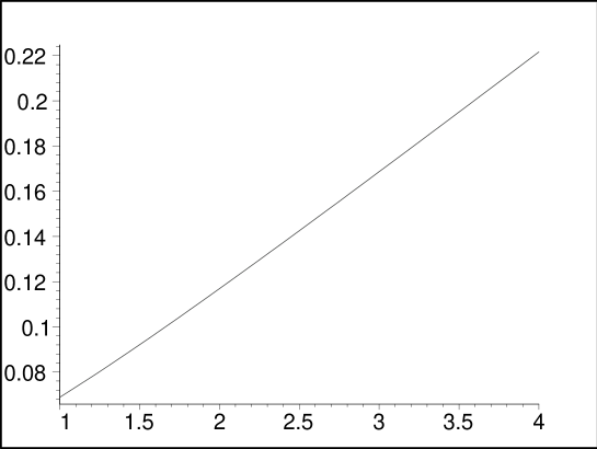
Figure 1: $C_{{\bf J},Q}$ versus $\Xi$ for $n=4$, $l=1$, $\beta=1$, $q=0.7$ and $r=0.8$.

IV CLOSING REMARKS

In this paper, we introduced a new class of charged, rotating solutions of $(n+1)$-dimensional Einstein-Born-Infeld gravity and investigate their properties. These solutions are asymptotically anti-de Sitter. In the particular case $\beta\rightarrow\infty$, these solutions reduce to the $(n+1)$-dimensional charged rotating black brane solutions given in Ref. Deh2 . We found that these solutions can represent black brane, with inner and outer event horizons, an extreme black brane or a naked singularity provided the parameters of the solutions are chosen suitably. We also computed thermodynamic quantities of the $(n+1)$-dimensional rotating charged black brane such as the temperature, entropy, charge, electric potential, mass and angular momentum and found that they satisfy the first law of thermodynamics. We found that these thermodynamic quantities are independent of the Born-Infeld parameter $\beta$.

Also, we studied the phase behavior of the charged rotating black branes in $(n+1)$ dimensions and showed that there is no Hawking-Page phase transition in spite of the charge and angular momenta of the branes. Indeed, we calculated the heat capacity and the determinant of the Hessian matrix of $M(S,{\bf J},Q)$ with respect to its extensive variables $S$, ${\bf J}$ and $Q$ of the black brane and found that they are positive for all the phase space, which means that the brane is stable for all the allowed values of the metric parameters. This phase behavior is in commensurable with the fact that there is no Hawking-Page transition for black object whose horizon is diffeomorphic to ${\mathbb{R}}^{p}$ and therefore the system is always in the high temperature phase Wit .

- (1) J. Maldacena, Adv. Theor. Math. Phys. 2, 231 (1998) [Int. J. Theor. Phys. 38, 1113 (1998)]; E. Witten, Adv. Theor. Math. Phys. 2, 253 (1998); O. Aharony, S. S. Gubser, J. Maldacena, H. Ooguri, and Y. Oz, Phys. Rep. 323, 183 (2000).
- (2) E. Witten, Adv. Theor. Math. Phys. 2, 505 (1998).
- (3) M. H. Dehghani and N. Farhangkhah, Phys. Rev. D 71, 044008 (2005); A. Sheykhi, M. H. Dehghani, N. Riazi and J. Pakravan, ibid. 74, 084816 (2006).
- (4) M. H. Dehghani, Phys. Rev. D 66, 044006 (2002); M. H. Dehghani and A. Khodam-Mohammadi, ibid. 67, 084006 (2003).
- (5) M. H. Dehghani and R. B. Mann, Phys. Rev. D 73, 104003 (2006); M. H. Dehghani, G. H. Bordbar and M. Shamirzaie ibid. 74, 064023 (2006).
- (6) M. Born and L. Infeld, Proc. Roy. Soc. Lond. A 144, 425 (1934).
- (7) B. Hoffmann, Phys. Rev. 47, 877 (1935).
- (8) E. S. Fradkin and A. A. Tseytlin, Phys. Lett. B 163, 123 (1985); E. Bergshoeff, E. Sezgin, C. N. Pope, and P. K. Townsend, Phys. Lett. B 188, 70 (1987); R. R. Metsaev, M. A. Rahmanov, and A. A. Tseytlin, Phys. Lett. B 193, 207 (1987); A. A. Tseytlin, Nucl. Phys. B 501, 41 (1997); D. Brecher and M. J. Perry, Nucl. Phys. B 527, 121 (1998).
- (9) M. Demianski, Found. Phys. 16, 187 (1986); D. Wiltshire, Phys. Rev. D 38, 2445 (1988); H. d Oliveira, Class. Quant. Grav. 11, 1469 (1994).
- (10) R.G. Cai, D.W. Pang and A. Wang, Phys.Rev. D 70, 124034 (2004).
- (11) T. K. Dey, Phys. Lett. B 595, 484 (2004).
- (12) J. P. S. Lemos, Class. Quantum Grav. 12, 1081 (1995); Phys. Lett. B 353, 46 (1995); J. P. S. Lemos and V. T. Zanchin, Phys. Rev. D 54, 3840 (1996).
- (13) A. M. Awad, Class. Quant. Grav. 20, 2827 (2003).
- (14) S. W. Hawking, Commun. Math. Phys. 25, 152 (1972); S. W. Hawking and G. F. R. Ellis, The Large Scale Structure of Spacetime (Cambridge University Press, 1973).
- (15) J. D. Beckenstein, Phys. Rev. D 7, 2333 (1973); S. W. Hawking, Nature (London) 248, 30 (1974); G. W. Gibbons and S. W. Hawking, Phys. Rev. D 15, 2738 (1977).
- (16) C. J. Hunter, Phys. Rev. D 59, 024009 (1999); S. W. Hawking, C. J. Hunter and D. N. Page, ibid. 59, 044033 (1999); R. B. Mann, ibid. 60, 104047 (1999); ibid. 61, 084013 (2000).
- (17) M. Cvetic and S. S. Gubser, J. High Energy Phys. 04, 024 (1999); M. M. Caldarelli, G. Cognola and D. Klemm, Class. Quantum Grav. 17, 399 (2000).