A non inflationary model with scale invariant cosmological perturbations

Abstract

We show that a contracting universe which bounces due to quantum cosmological effects and connects to the hot big-bang expansion phase, can produce an almost scale invariant spectrum of perturbations provided the perturbations are produced during an almost matter dominated era in the contraction phase. This is achieved using Bohmian solutions of the canonical Wheeler-de Witt equation, thus treating both the background and the perturbations in a fully quantum manner. We find a very slightly blue spectrum ($n_{{}_{\mathrm{S}}}-1>0$). Taking into account the spectral index constraint as well as the CMB normalization measure yields an equation of state that should be less than $\omega\lesssim 8\times 10^{-4}$, implying $n_{{}_{\mathrm{S}}}-1\sim\mathcal{O}\left(10^{-4}\right)$, and that the characteristic size of the Universe at the bounce is $L_{0}\sim 10^{3}\ell_{{}_{\mathrm{Pl}}}$, a region where one expects that the Wheeler-DeWitt equation should be valid without being spoiled by string or loop quantum gravity effects.

I Introduction

When the theory of cosmological perturbations [1] is applied to a background cosmological model and their initial spectra can be justified in physical terms, as it is the case of inflationary and nonsingular models where the horizon problem is solved, one obtains definite predictions concerning the spectrum of primordial scalar and tensor perturbations in this background, establishing the initial conditions for structure formation and the angular power spectrum of the anisotropies of the cosmic microwave background radiation (CMBR). Since the release of the first data obtained from observations of these anisotropies in 1992 [2], primordial cosmological models have been confronted with new observational facts [3], bringing them definitely out of the arena of speculations based almost uniquely on theoretical and æsthetical arguments. In fact, many interesting cosmological backgrounds have been falsified since then [4], while the inflationary paradigm [5] has, on the contrary, been widely confirmed and is now accepted as part of the “standard” model of cosmology.

Some of the primordial cosmological backgrounds proposed in the literature are quantum cosmological models which share the attractive properties of exhibiting neither singularities nor horizons [6, 7, 8], leading the universe evolution through a bouncing phase due to quantum effects, and a contracting phase before the bounce. They constitute an example of a bouncing model, a possibility that has attracted the attention of many authors [9], without the presence of any phantom field. These features of the background introduce a new picture for the evolution of cosmological perturbations: vacuum initial conditions may now be imposed when the Universe was very big and almost flat, and effects due to the contracting and bouncing phases, which are not present in the standard background cosmological model, may change the subsequent evolution of perturbations in the expanding phase. Hence, it is quite important to study the evolution of perturbations in these quantum backgrounds to confront them with the data.

The present paper is the fourth of a series [10, 11, 12] where the theory of cosmological perturbations is obtained and simplified without assuming any dynamics satisfied by the background. This is a necessary prerequisite if one wants to study the propagation of perturbations on a quantized background. The usual theory of cosmological perturbations with their simple equations [1] relies essentially on the assumptions that the background is described by pure classical General Relativity (GR), while the perturbations thereof stem from quantum fluctuations. It is a semiclassical approach, where the background is classical and the perturbations are quantized. A full quantum treatment of both background and perturbations has already been constructed in Ref. [13], but rather complicated equations were obtained, even at first order, due to the fact that the background does not satisfy classical Einstein’s equations. In Refs. [10, 12], we have managed to put these complicated equations in simple forms, very similar to the equations obtained in Ref. [1], through the implementation of canonical transformations and redefinitions of the lapse function without ever using the background classical equations. These expressions happen to become identical to those of  [1] when the background behaves as a pre-determined function of time, which is perfectly consistent with the idea of quantization if we work with an ontological interpretation of quantum mechanics [14]. In Ref. [11], these results have been applied to obtain the possible power spectra of tensor perturbations in different quantum cosmological models using an hydrodynamical description. The aim of this paper is to apply the results of Ref. [12] to obtain the power spectra of scalar perturbations in such quantum models and confront the results with observational data [3].

The paper is organized as follows. In Sec. II we summarize the results of Refs. [12] obtaining the simple equations which govern the dynamics of quantum perturbations in the quantum backgrounds of Refs. [6, 8]. In Sec. III we obtain the spectral index for long wavelengths of scalar perturbations in these quantum backgrounds, and in Sec. IV we confirm these results numerically, also obtaining their amplitude and constraining the free parameters of the theory with observational data. We end in Sec. V with conclusions and discussions.

II Quantization of the background and perturbations

The action we shall begin with is that of General Relativity (GR) with a perfect fluid, the latter being described as in Ref. [1], i.e.

$$\mathcal{S}=\mathcal{S}_{{}_{\mathrm{GR}}}+\mathcal{S}_{\mathrm{fluid}}=-\frac{1}{6\ell_{{}_{\mathrm{Pl}}}^{2}}\int\sqrt{-g}R\mbox{d}^{4}x-\int\sqrt{-g}\epsilon\mbox{d}^{4}x,$$ (1)

where $\ell_{{}_{\mathrm{Pl}}}=(8\pi G_{{}_{\mathrm{N}}}/3)^{1/2}$ is the Planck length in natural units ($\hbar=c=1$), $\epsilon$ is the perfect fluid energy density whose pressure $p$ is provided by the relation $p=\omega\epsilon$, $\omega$ being a nonvanishing constant.

Let the geometry of spacetime be given by

$$g_{\mu\nu}=g^{(0)}_{\mu\nu}+h_{\mu\nu},$$ (2)

where $g^{(0)}_{\mu\nu}$ represents a homogeneous and isotropic cosmological background,

$$\mbox{d}s^{2}=g^{(0)}_{\mu\nu}\mbox{d}x^{\mu}\mbox{d}x^{\nu}=N^{2}(t)\mbox{d}t^{2}-a^{2}(t)\delta_{ij}\mbox{d}x^{i}\mbox{d}x^{j},$$ (3)

where we are restricted to a flat spatial metric, and the $h_{\mu\nu}$ represents linear scalar perturbations around it which we decompose into

$$h_{00} = 2N^{2}\phi$$

$$h_{0i} = -NaB_{,i}$$ (4)

$$h_{ij} = 2a^{2}(\psi\gamma_{ij}-E_{,ij}).$$

Substituting Eqs. (II) and (3) into the Einstein-Hilbert action (1), performing Legendre and canonical transformations, redefining $N$ with terms which do not alter the equations of motion up to first order, all this without ever using the background equations of motion, the Hamiltonian up to second order is simplified to (see Ref. [12] for details)

$$H=N\left[H_{0}^{(0)}+H_{0}^{(2)}\right]+\Lambda_{N}P_{N}+\int\mbox{d}^{3}x\phi\pi_{\psi}+\int\mbox{d}^{3}x\Lambda_{\phi}\pi_{\phi},$$ (5)

where

$$H_{0}^{(0)}\equiv-\frac{l^{2}P_{a}^{2}}{4aV}+\frac{P_{T}}{a^{3\omega}},$$ (6)

and

$$H_{0}^{(2)}\equiv\frac{1}{2a^{3}}\int\mbox{d}^{3}x\pi^{2}+\frac{a\omega}{2}\int\mbox{d}^{3}xv^{,i}v_{,i}.$$ (7)

The quantities $N$, $\phi$, $\Lambda_{N}$ and $\Lambda_{\phi}$ play the role of Lagrange multipliers of the constraints $H_{0}^{(0)}+H_{0}^{(2)}\approx 0$, $\pi_{\psi}\approx 0$, $P_{N}\approx 0$, and $\pi_{\phi}\approx 0$, respectively. The momenta $P_{a}$, $\pi_{\phi}$, $\pi_{\psi}$, $P_{N}$ and $P_{T}$ are conjugate respectively to $a,\phi,\psi,N,T$, this last variable playing the role of time.

The variable $v$ is related with the gauge invariant Bardeen potential $\Phi$ (see Ref. [12]) through

$$\Phi^{,i}\,_{,i}=-\frac{3\ell_{{}_{\mathrm{Pl}}}^{2}\sqrt{(\omega+1)\epsilon_{0}}}{2\sqrt{\omega}}a\biggl{(}\frac{v}{a}\biggr{)}^{\prime},$$ (8)

which coincides with equation (12.8) of Ref. [1] relating $v$ and $\Phi$

$$\Phi^{,i}\,_{,i}=-\sqrt{\frac{3}{2}}\frac{\ell_{{}_{\mathrm{Pl}}}{\cal H}\gamma}{c_{\mathrm{s}}^{2}}\left(\frac{v}{z}\right)^{\prime},$$ (9)

where

$$\gamma\equiv 1-\frac{{\cal H}^{\prime}}{{\cal H}^{2}},\ \ \ \ z\equiv\frac{a}{c_{\mathrm{s}}}\sqrt{\gamma},$$ (10)

and $c_{\mathrm{s}}$ ($c^{2}_{\mathrm{s}}\equiv\mbox{d}p_{0}/\mbox{d}\epsilon_{0}=p_{0}^{\prime}/\epsilon_{0}^{\prime}$) is the velocity at which density perturbations propagates, and when the classical equations of motion, that can be recast in the form

$$\epsilon_{0}+p_{0}=\epsilon_{0}(1+\omega)=\frac{2{\cal H}^{2}\gamma}{3\ell_{{}_{\mathrm{Pl}}}^{2}a^{2}},$$

are used.

The above quantities have been redefined in order to be dimensionless. For instance, the physical scale factor $a_{\rm phys}$ can be obtained from the dimensionless $a$ present in (6) through $a_{\rm phys}=\ell_{{}_{\mathrm{Pl}}}a/\sqrt{V}$, where $V$ is the comoving volume of the background spacelike hypersurfaces, which we suppose to be compact. The constraint $H_{0}^{(0)}+H_{0}^{(2)}$ is the one which generates the dynamics, yielding the correct Einstein equations both at zeroth and first order in the perturbations, as can be checked explicitly. The others imply that $N$, $\phi$, and $\psi$ are not relevant. The unique perturbed degree of freedom is $v$, as obtained in Ref. [1]. We would like to emphasize again that in order to obtain the above results, no assumption has been made about the background dynamics: Hamiltonian (5) is ready to be applied in the quantization procedure.

In the Dirac quantization procedure, the first class constraints must annihilate the wave functional $\Psi\left[N,a,\phi(x^{i}),\psi(x^{i}),v(x^{i}),T\right]$, yielding

$$\frac{\partial}{\partial N}\Psi=\frac{\delta}{\delta\phi}\Psi=\frac{\delta}{\delta\psi}\Psi=H\Psi=0.$$ (11)

The first three equations impose that the wave functional does not depend on $N$, $\phi$ and $\psi$: as mentioned above, $N$ and $\phi$ are, respectively, the homogeneous and inhomogeneous parts of the total lapse function, which are just Lagrange multipliers of constraints, and $\psi$ has been substituted by $v(x^{i})$, the unique degree of freedom of scalar perturbations, as expected.

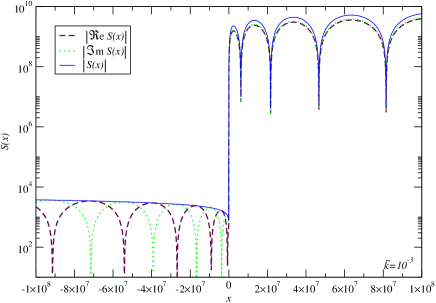
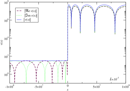
Figure 1: Time evolution of the scalar mode function for the equation of state $\omega=0.1$ in the one-fluid model of the bounce. The left panel shows the full time evolution which was computed, i.e., the function $S(x)$, while the right panel shows $v(x)$ itself, both plots having $\tilde{k}=10^{-3}$. For $x<0$, there are oscillations only in the real and imaginary parts of the mode, so the amplitude shown is a non oscillating function of time. It however acquires an oscillating piece after the bounce has taken place.

As $P_{T}$ appears linearly in $H$, and making the gauge choice $N=a^{3\omega}$, one can interpret the $T$ variable as a time parameter. Hence, the equation

$$H\Psi=0$$ (12)

assumes the Schrödinger form

$$i\frac{\partial}{\partial T}\Psi = \frac{1}{4}\left\{a^{(3\omega-1)/2}\frac{\partial}{\partial a}\left[a^{(3\omega-1)/2}\frac{\partial}{\partial a}\right]\right\}\Psi$$ (13)

$$- \frac{a^{3\omega-1}}{2}\int\mbox{d}^{3}x\frac{\delta^{2}}{\delta v^{2}}\Psi+\frac{a^{3\omega+1}\omega}{2}\int\mbox{d}^{3}xv^{,i}v_{,i}\Psi,$$

where we have chosen the factor ordering in $a$ in order to yield a covariant Schrödinger equation under field redefinitions.

If one makes the ansatz

$$\Psi[a,v,T]=\Psi_{(0)}(a,T)\Psi_{(2)}[a,v,T],$$ (15)

where $\Psi_{(0)}(a,T)$ satisfies the equation

$$i\frac{\partial}{\partial T}\Psi_{(0)}(a,T)=\frac{a^{(3\omega-1)/2}}{4}\frac{\partial}{\partial a}\left[a^{(3\omega-1)/2}\frac{\partial}{\partial a}\right]\Psi_{(0)}(a,T),$$ (16)

then we obtain for $\Psi_{(2)}[a,v,T]$ the equation.

$$i\frac{\partial}{\partial T}\Psi_{(2)}(a,v,T) = -\frac{a^{(3\omega-1)}}{2}\int\mbox{d}^{3}x\frac{\delta^{2}}{\delta v^{2}}\Psi_{(2)}(a,v,T)$$

$$+ \frac{\omega a^{(3\omega+1)}}{2}\int\mbox{d}^{3}xv^{,i}v_{,i}\Psi_{(2)}(a,v,T).$$

Terms involving $\Psi_{(2)}(a,v,T)$ can be neglected in Eq. (16), either through a judicious choice of the $a$ dependence of $\Psi_{(2)}$ [11], or because quantum perturbations initiated in a vacuum quantum state should not contribute to it [13]. In another perspective, using the Bohmian approach [14], one can write $\Psi[a,v,T]=\Psi_{(0)}(a,T)\Psi_{(2)}[v,T]$ and consider $a(T)$ appearing in the equation for $\Psi_{(2)}[v,T]$ as a prescribed function of time, the quantum Bohmian trajectory, obtained from the zeroth order equation for $\Psi_{(0)}(a,T)$.

Going on with the ontological Bohm-de Broglie interpretation of quantum mechanics, where quantum trajectories can be defined, Eq. (II) can be further simplified if one uses Eq.  (16) to obtain background quantum Bohmian trajectories $a(T)$ as in Refs. [6, 7, 8]. This can be done as follows: we change variables to

$$\chi=\frac{2}{3}(1-\omega)^{-1}a^{3(1-\omega)/2},$$

obtaining the simple equation

$$i\frac{\partial\Psi_{(0)}(a,T)}{\partial T}=\frac{1}{4}\frac{\partial^{2}\Psi_{(0)}(a,T)}{\partial\chi^{2}}.$$ (18)

This is just the time reversed Schrödinger equation for a one dimensional free particle constrained to the positive axis. As $a$ and $\chi$ are positive, solutions which have unitary evolution must satisfy the condition

$$\Psi_{(0)}^{\star}\frac{\partial\Psi_{(0)}}{\partial\chi}-\Psi_{(0)}\frac{\partial\Psi_{(0)}^{\star}}{\partial\chi}\Biggl{|}_{\chi=0}=0$$ (19)

(see Ref. [8] for details). We will choose the initial normalized wave function

$$\Psi_{(0)}^{(\mathrm{init})}(\chi)=\biggl{(}\frac{8}{T_{0}\pi}\biggr{)}^{1/4}\exp\left(-\frac{\chi^{2}}{T_{0}}\right),$$ (20)

where $T_{0}$ is an arbitrary constant. The Gaussian $\Psi_{(0)}^{(\mathrm{init})}$ satisfies condition (19).

Using the propagator procedure of Refs. [6, 8], we obtain the wave solution for all times in terms of $a$:

$$\Psi_{(0)}(a,T)=\left[\frac{8T_{0}}{\pi\left(T^{2}+T_{0}^{2}\right)}\right]^{1/4}\exp\biggl{[}\frac{-4T_{0}a^{3(1-\omega)}}{9(T^{2}+T_{0}^{2})(1-\omega)^{2}}\biggr{]}\exp\left\{-i\left[\frac{4Ta^{3(1-\omega)}}{9(T^{2}+T_{0}^{2})(1-\omega)^{2}}+\frac{1}{2}\arctan\biggl{(}\frac{T_{0}}{T}\biggr{)}-\frac{\pi}{4}\right]\right\}.$$ (21)

Due to the chosen factor ordering, the probability density $\rho(a,T)$ has a non trivial measure and it is given by $\rho(a,T)=a^{(1-3\omega)/2}\left|\Psi_{(0)}(a,T)\right|^{2}$. Its continuity equation coming from Eq. (18) reads

$$\frac{\partial\rho}{\partial T}-\frac{\partial}{\partial a}\biggl{[}\frac{a^{(3\omega-1)}}{2}\frac{\partial S}{\partial a}\rho\biggr{]}=0,$$ (22)

which implies in the Bohm interpretation that

$$\dot{a}=-\frac{a^{(3\omega-1)}}{2}\frac{\partial S}{\partial a},$$ (23)

in accordance with the classical relations $\dot{a}=\{a,H\}=-a^{(3\omega-1)}P_{a}/2$ and $P_{a}=\partial S/\partial a$.

Inserting the phase of (21) into Eq. (23), we obtain the Bohmian quantum trajectory for the scale factor:

$$a(T)=a_{0}\left[1+\left(\frac{T}{T_{0}}\right)^{2}\right]^{\frac{1}{3(1-\omega)}}.$$ (24)

Note that this solution has no singularities and tends to the classical solution when $T\rightarrow\pm\infty$. Remember that we are in the gauge $N=a^{3\omega}$, and $T$ is related to conformal time through

$$N\mbox{d}T=a\mbox{d}\eta\quad\Longrightarrow\mbox{d}\eta=\left[a(T)\right]^{3\omega-1}\mbox{d}T.$$ (25)

The solution (24) can be obtained for other initial wave functions (see Ref. [8]).

The Bohmian quantum trajectory $a(T)$ can be used in Eq. (II). Indeed, since one can view $a(T)$ as a function of $T$, it is possible to implement the time dependent canonical transformation generated by

$$U = \exp\left[i\left(\int\mbox{d}^{3}x\frac{\dot{a}v^{2}}{2a}\right)\right]\times$$ (27)

$$\times\exp\left\{i\left[\int\mbox{d}^{3}x\left(\frac{v\pi+\pi v}{2}\right)\ln\left(\frac{1}{a}\right)\right]\right\}.$$

As $a(T)$ is a given quantum trajectory coming from Eq. (18), Eq. (27) must be viewed as the generator of a time dependent canonical transformation to Eq. (18). It yields, in terms of conformal time, the equation for $\Psi_{(2)}[v,a(\eta),\eta]$

$$i\frac{\partial\Psi_{(2)}}{\partial\eta}=\int\mbox{d}^{3}x\left(-\frac{1}{2}\frac{\delta^{2}}{\delta v^{2}}+\frac{\omega}{2}v_{,i}v^{,i}-\frac{{a^{\prime\prime}}}{2a}v^{2}\right)\Psi_{(2)}.$$ (28)

This is the most simple form of the Schrödinger equation which governs scalar perturbations in a quantum minisuperspace model with fluid matter source. The corresponding time evolution equation for the operator $v$ in the Heisenberg picture is given by

$$v^{\prime\prime}-\omega v^{,i}_{\ ,i}-\frac{a^{\prime\prime}}{a}v=0,$$ (29)

where a prime means derivative with respect to conformal time. In terms of the normal modes $v_{k}$, the above equation reads

$$v^{\prime\prime}_{k}+\biggl{(}\omega k^{2}-\frac{{a^{\prime\prime}}}{a}\biggr{)}v_{k}=0.$$ (30)

These equations have the same form as the equations for scalar perturbations obtained in Ref. [1]. This is quite natural since for a single fluid with constant equation of state $\omega$, the pump function $z^{\prime\prime}/z$ obtained in Ref. [1] is exactly equal to $a^{\prime\prime}/a$ obtained here. The difference is that the function $a(\eta)$ is no longer a classical solution of the background equations but a quantum Bohmian trajectory of the quantized background, which may lead to different power spectra.

III Spectrum of scalar perturbations in quantum cosmological models

Having obtained in the previous section the propagation equation for the full quantum scalar modes, namely Eq. (30), in the Bohmian picture with the scale factor assuming the form (24), it is our goal now to solve this equation in order to obtain the scalar perturbation power spectrum as predicted by such models. In this section we obtain the analytical result for long wavelength perturbations through a matching procedure, while in the following we confirm our current findings by getting numerical solutions.

We shall begin with the asymptotic behaviors. When $|T|\gg|T_{0}|$, far from the bounce, one can write Eq. (30) as

$$v^{\prime\prime}+\left[\omega k^{2}+\frac{2(3\omega-1)}{(1+3\omega)^{2}\eta^{2}}\right]\mu=0,$$ (31)

whose solution is

$$v=\sqrt{\eta}\left[c_{1}(k)H^{(1)}_{\nu}(\bar{k}\eta)+c_{2}(k)H^{(2)}_{\nu}(\bar{k}\eta)\right],$$ (32)

with

$$\nu=\frac{3(1-\omega)}{2(3\omega+1)},$$

$c_{1}$ and $c_{2}$ being two constants depending on the wavelength, $H^{(1,2)}$ being Hankel functions, and $\bar{k}\equiv\sqrt{\omega}k$.

This solution applies asymptotically, where one can impose vacuum initial conditions as in [1]

$$v_{\mathrm{ini}}=\frac{\mbox{e}^{i\bar{k}\eta}}{\sqrt{\bar{k}}},$$ (33)

which implies that

$$c_{1}=0\quad\hbox{and}\quad c_{2}=\ell_{{}_{\mathrm{Pl}}}\sqrt{\frac{3\pi}{2}}\mbox{e}^{-i\frac{\pi}{2}\left(\nu+\frac{1}{2}\right)}.$$

The solution can also be expanded in powers of $k^{2}$ according to the formal solution [1]

$$\frac{v}{a} \simeq A_{1}(k)\biggl{[}1-\omega k^{2}\int^{t}\frac{\mbox{d}\bar{\eta}}{a^{2}\left(\bar{\eta}\right)}\int^{\bar{\eta}}a^{2}\left(\bar{\bar{\eta}}\right)\mbox{d}\bar{\bar{\eta}}\biggr{]}$$ (34)

$$+ A_{2}(k)\biggl{[}\int^{\eta}\frac{\mbox{d}\bar{\eta}}{a^{2}}-\omega k^{2}\int^{\eta}\frac{\mbox{d}\bar{\eta}}{a^{2}}\int^{\bar{\eta}}a^{2}\mbox{d}\bar{\bar{\eta}}\int^{\bar{\bar{\eta}}}\frac{\mbox{d}\bar{\bar{\bar{\eta}}}}{a^{2}}\biggr{]},$$

up to order $\mathcal{O}(k^{j\geq 4})$ terms. In Eq. (LABEL:solform), the coefficients $A_{1}$ and $A_{2}$ are two constants depending only on the wavenumber $k$ through the initial conditions. Although this form is particularly valid as long as $\omega k^{2}\ll a^{\prime\prime}/a$, i.e. when the mode is below its potential, Eq. (LABEL:solform) should formally apply for all times. In the matching region $\omega k^{2}\approx a^{\prime\prime}/a$, the $\mathcal{O}(k^{2})$ terms may give contributions to the amplitude, but they do not alter the $k$-dependence of the power spectrum.

For the solution (24), the leading order of the solution (LABEL:solform) reads

$$\frac{v}{a} = A_{1}+A_{2}T_{0}a_{0}^{3(\omega-1)}\left(\arctan x+\frac{\pi}{2}\right)$$ (36)

$$\sim A_{1}-A_{2}T_{0}a_{0}^{3(\omega-1)}\frac{1}{x},$$ (37)

where

$$x\equiv\frac{T}{T_{0}}.$$

In the last step we have taken the limit $x\to-\infty$, and the constant $\pi/2$ was introduced in order for $A_{1}$ represent the constant mode when it enters the potential.

Propagating this solution to the other side of the bounce, in the expanding epoch, i.e. the limit for $x\to+\infty$, yields

$$\frac{v}{a} \sim A_{1}+\biggl{(}\pi-\frac{1}{x}\biggr{)}a_{0}^{3(\omega-1)}T_{0}A_{2}$$ (38)

$$= \left(A_{1}+\pi a_{0}^{3(\omega-1)}T_{0}A_{2}\right)+\frac{1}{x}a_{0}^{3(\omega-1)}T_{0}A_{2}.$$ (39)

Note that there is a mixing in the constant part of the mode when it passes through the bounce. Hence, in these types of bouncing models, the bounce has important consequences for the final power spectrum.

In order to find the $k$-dependence of $A_{1}$ and $A_{2}$, we match $v$ and $v^{\prime}$ in Eqs. (37) and (32), obtaining, to leading order,

$$A_{1} = \left[\frac{3\omega-1}{3\alpha\left(\omega-1\right)}\tilde{C}+a_{0}^{3\omega-1}T_{0}\beta\tilde{D}\right]\biggl{(}\frac{\bar{k}}{k_{0}}\biggr{)}^{\frac{3\left(1-\omega\right)}{2\left(3\omega+1\right)}},$$ (40)

$$A_{2} = -\left[\frac{2a_{0}^{1+3\omega}}{3\beta\left(1-\omega\right)T_{0}}\tilde{C}-\alpha\tilde{D}\right]\biggl{(}\frac{\bar{k}}{k_{0}}\biggr{)}^{\frac{3\left(\omega-1\right)}{2\left(3\omega+1\right)}},$$ (41)

from which stem the spectral behaviors

$$A_{1}\propto k^{\frac{3\left(1-\omega\right)}{2\left(3\omega+1\right)}},\ \ \ \ A_{2}\propto k^{\frac{3\left(\omega-1\right)}{2\left(3\omega+1\right)}},$$ (42)

with

$$\alpha=\left[\frac{9\left(1-\omega\right)^{2}}{2\left|1-3\omega\right|}\right]^{-1/(1+3\omega)},\ \ \ \ \beta=\left[\frac{9\left(1-\omega\right)^{2}}{2\left|1-3\omega\right|}\right]^{\frac{1-3\omega}{2(1+3\omega)}},$$

$$\tilde{C}=\sqrt{T_{0}}a_{0}^{(3\omega-1)/2}c_{2}\sqrt{k\eta_{{}_{\mathrm{M}}}}H_{\nu}^{(2)}(k\eta_{{}_{\mathrm{M}}}),$$ (43)

and

$$\tilde{D} = a_{0}^{(1-3\omega)/2}T_{0}^{-1/2}\frac{c_{2}}{2}\Bigg{\{}\frac{H_{\nu}^{(2)}(\bar{k}\eta_{{}_{\mathrm{M}}})}{\sqrt{\bar{k}\eta_{{}_{\mathrm{M}}}}}$$ (45)

$$\hskip 8.53581pt+\sqrt{\bar{k}\eta_{{}_{\mathrm{M}}}}\left[H_{\nu-1}^{(2)}(\bar{k}\eta_{{}_{\mathrm{M}}})-H_{\nu+1}^{(2)}(\bar{k}\eta_{{}_{\mathrm{M}}})\right]\bigg{\}},$$

with

$$k\eta_{{}_{\mathrm{M}}}=\frac{\sqrt{2|1-3\omega|}}{1+3\omega}$$

and

$$k^{-1}_{0}=T_{0}a_{0}^{3\omega-1}.$$ (46)

The coefficients $A_{1}$ and $A_{2}$ each contain a power-law behavior in $k$. Because $0<\omega<1$, the power in $A_{2}$ [Eq. (41)] is negative definite and that in $A_{1}$ [Eq. (40)] is positive definite. Therefore, $A_{2}$ is the dominant mode, while $A_{1}$ provides the sub-dominant mode.

The relation between the Bardeen potential $\Phi$ and $v$ is given by Eq. (8). Using Eqs. (LABEL:solform), (24) and (25) in order to change variables to $x$, Eq. (8) leads to

$$\Phi a^{(1+3\omega)/2}\propto\biggl{(}\frac{v}{a}\biggr{)}^{\prime}=-\omega k^{2}\frac{{A}_{1}(k)}{a^{2}}\int^{x}T_{0}a^{2}\left(\bar{x}\right)\mbox{d}\bar{x}$$

$$+ \frac{{A}_{2}(k)}{a^{2}}\biggl{[}1-\omega k^{2}\int^{x}\mbox{d}\bar{x}a^{2}\int^{\bar{x}}\frac{T_{0}^{2}}{a_{0}^{2}(1+{\bar{\bar{x}}})^{2}}\mbox{d}\bar{\bar{x}}\biggr{]}+\mathcal{O}(k^{4})$$

$$\simeq -\omega k^{2}\frac{{A}_{1}(k)}{a^{2}}\int^{x}T_{0}a^{2}\left(\bar{x}\right)\mbox{d}\bar{\eta}$$

$$+ \frac{{A}_{2}(k)}{a^{2}}\biggl{[}1-\omega k^{2}\frac{T_{0}^{2}}{a_{0}^{2}}\int^{x}\mbox{d}\bar{x}a^{2}(\arctan\bar{x}+\pi/2)\biggr{]},$$

where the constant $\pi/2$ was introduced when performing the last integral in order for ${A}_{1}$ to represent the constant mode at large negative values of $x$ when $v_{k}$ is entering the potential, as before. At large positive values of $x$, when $v_{k}$ is leaving the potential and $x\propto\eta^{3(1-\omega)/(1+3\omega)}$, the constant mode of $\Phi$, like $v$, mixes $A_{1}$ with $A_{2}$. In this region, taking into account that $A_{2}$ dominates over $A_{1}$, we obtain:

$$\Phi\propto k^{\frac{3\left(\omega-1\right)}{2\left(3\omega+1\right)}}\biggl{[}\mathrm{const.}+\frac{1}{\eta^{(5+3\omega)/(1+3\omega)}}\biggr{]}.$$ (48)

The power spectrum

$$\mathcal{P}_{\Phi}\equiv\frac{2k^{3}}{\pi^{2}}\left|\Phi\right|^{2},$$ (49)

then reads

$$\mathcal{P}_{\Phi}\propto k^{n_{{}_{\mathrm{S}}}-1},$$ (50)

and we get

$$n_{{}_{\mathrm{S}}}=1+\frac{12\omega}{1+3\omega}.$$ (51)

For gravitational waves (see Ref. [11] for details), the equation for the modes $\mu=h/a$ reads

$$\mu^{\prime\prime}+\left(k^{2}+2{\cal K}-\frac{a^{\prime\prime}}{a}\right)\mu=0,$$ (52)

yielding the power spectrum for long wavelengths:

$$\mathcal{P}_{h}\equiv\frac{2k^{3}}{\pi^{2}}\left|\frac{\mu}{a}\right|^{2}.$$ (53)

In Ref. [11], we have obtained

$$\mathcal{P}_{h}\propto k^{n_{{}_{\mathrm{T}}}},$$ (54)

with, as for the scalar modes,

$$n_{{}_{\mathrm{T}}}=\frac{12\omega}{1+3\omega}.$$ (55)

Note that in the limit $\omega\rightarrow 0$ (dust) we obtain a scale invariant spectrum for both tensor and scalar perturbations. This result will be confirmed in the next section through numerical calculations which will also give the amplitudes. However, it is not necessary that the fluid that dominates during the bounce be dust. The dependencies on $k$ of $A_{1}$ and $A_{2}$ are obtained far from the bounce, and they should not change in a transition, say, from matter to radiation domination in the contraction phase, or during the bounce. The effect of the bounce is essentially to mix these two coefficients in order for the constant mode to acquire the scale invariant piece. Hence, the bounce may be dominated by another fluid, like radiation. If while entering the potential the fluid that dominates is dust-like, then the spectrum should be almost scale invariant. Note also that since we assume an ordinary matter fluid, the equation of state is positive definite, being, in the most pressure-less case, obtained as a result of the quantum non vanishing mean square velocity. Thus, we do expect a blue spectrum.

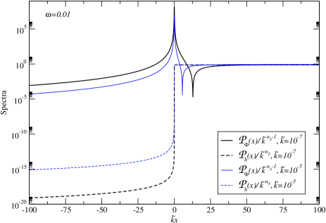
Figure 2: Rescaled power spectra for scalar and tensor perturbations as functions of time for $\omega=0.01$ and two different values of $\tilde{k}$. It is clear from the figure that not only both spectra reach a constant mode, but also that this mode does behave as indicated in Eqs. (51) and (55). It is purely incidental that the actual constant value of both modes are very close for that particular value of $\omega$. The constant values obtained in this figure are the one used to derive the spectrum below. In this figure and the following, the value of $n_{{}_{\mathrm{S}}}$ used to rescale $\Phi$ is the one derived in Eq. (51), thus proving the validity of the analytic calculation.

IV Numerical results

In this section we will confirm the spectral indices of scalar perturbations obtained above, and obtain the amplitude of the scale invariant mode. The dynamical mode equation is expressible in terms of the function $S\equiv a^{\frac{1}{2}(1-3\omega)}v/\sqrt{T_{0}}$ (the constant $\sqrt{T_{0}}$ being introduced in order for $S$ to be dimensionless), namely [11]

$$\ddot{S}+\left[\tilde{k}^{2}\left(1+x^{2}\right)^{\frac{2(3\omega-1)}{3(1-\omega)}}-\frac{1}{\left(1+x^{2}\right)^{2}}\right]S=0,$$ (56)

with, in this latter case, $x\equiv T/T_{0}$ and $\tilde{k}\equiv c_{\mathrm{s}}kT_{0}/a_{0}^{1-3\omega}$. We can apply the vacuum initial conditions

$$v_{\mathrm{ini}}=\frac{\mbox{e}^{ic_{\mathrm{s}}k\eta}}{\sqrt{c_{\mathrm{s}}k}},$$ (57)

with the sound velocity $c_{\mathrm{s}}=\sqrt{\omega}$ a constant. It is clear here that one must insist upon not having $\omega=0$ in order to be able to put these initial conditions. Again, anyway, the sound velocity, even in a matter dominated phase, is not expected to be vanishing identically.

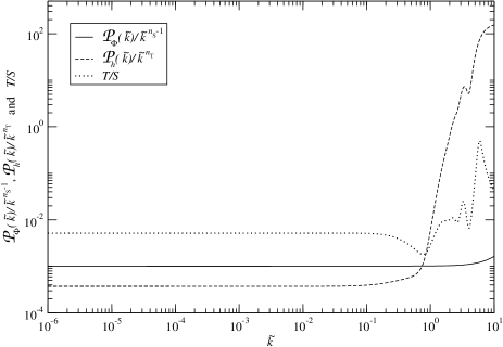
Figure 3: Rescaled power spectra for $\omega=8\times 10^{-4}$, corresponding to the conservative maximum bound on the deviation from a scale invariant spectrum $n_{{}_{\mathrm{S}}}=1.01$, as function of $k$. The scalar spectrum $\mathcal{P}_{\Phi}$ is the full line, while the dashed line is the gravitational wave spectrum $\mathcal{P}_{h}$. Also shown is the ratio $T/S$ (dotted); in this case, the $T/S\simeq 5.2\times 10^{-3}$, i.e. almost two orders of magnitude below the current limit. This case has a typical bounce length-scale of $L_{0}\sim 1.47\times 10^{3}\ell_{{}_{\mathrm{Pl}}}$. The amplitude of the modes is obtained as the constant part of Fig. 2.

Defining

$$L_{0}=T_{0}a_{0}^{3\omega},$$ (58)

the curvature scale at the bounce (the characteristic bounce length-scale), namely, $L_{0}\propto 1/\sqrt{R_{0}}$ where $R_{0}$ is the scalar curvature at the bounce, from which one can write

$$\tilde{k}=\frac{k}{a_{0}}L_{0}\equiv\frac{L_{0}}{\lambda_{\mathrm{phys}}^{\mathrm{bounce}}},$$ (59)

one obtains the scalar perturbation density spectrum as a function of time through

$$\mathcal{P}_{\Phi}=\frac{2(\omega+1)}{\pi^{2}\sqrt{\omega}\left(1-\omega\right))^{2}\tilde{k}}|f(x)|^{2}\left(\frac{\ell_{{}_{\mathrm{Pl}}}}{L_{0}}\right)^{2},$$ (60)

where

$$f(x)\equiv\left(1+x^{2}\right)^{-\frac{1+3\omega}{3(1-\omega)}}\frac{\mbox{d}S}{\mbox{d}x}-x\left(1+x^{2}\right)^{-\frac{4}{3(1-\omega)}}S,$$

while the tensor power spectrum is

$$\mathcal{P}_{h}=\frac{2\tilde{k}^{3}}{\pi^{2}}\frac{|\bar{v}|^{2}}{1+x^{2}}\left(\frac{\ell_{{}_{\mathrm{Pl}}}}{L_{0}}\right)^{2},$$ (61)

in which the rescaled function $\bar{v}$, defined through [11]

$$\bar{v}\equiv\frac{a^{\frac{1}{2}(1-3\omega)}\mu}{\ell_{{}_{\mathrm{Pl}}}\sqrt{T_{0}}},$$

satisfies the same dynamical equation (56) with $c_{\mathrm{s}}\to 1$, with $\mu$ subject to initial condition

$$\mu_{\mathrm{ini}}=\sqrt{\frac{3}{k}}\ell_{{}_{\mathrm{Pl}}}\mbox{e}^{-ik\eta}.$$ (62)

From the above defined spectra, one reads the amplitudes

$$A_{{}_{\mathrm{S}}}^{2}\equiv\frac{4}{25}\mathcal{P}_{\zeta}$$ (63)

and

$$A_{{}_{\mathrm{T}}}^{2}\equiv\frac{1}{100}\mathcal{P}_{h},$$ (64)

where we assume the classical relation between $\Phi$ and the curvature perturbation $\zeta$ through

$$\zeta=\frac{5+3\omega}{3(1+\omega)}\Phi\ \ \to\ \ \mathcal{P}_{\zeta}=\left[\frac{5+3\omega}{3(1+\omega)}\right]^{2}\mathcal{P}_{\Phi},$$ (65)

to obtain the observed spectrum. Since both spectra are identical power laws, and indeed almost scale invariant power laws, the tensor-to-scalar ($T/S$) ratio, defined by the CMB multipoles $C_{\ell}$ at $\ell=10$ as

$$\frac{T}{S}\equiv\frac{C_{10}^{\mathrm{(T)}}}{C_{10}^{\mathrm{(S)}}}=\mathcal{F}(\Omega,\cdots)\frac{A_{{}_{\mathrm{T}}}^{2}}{A_{{}_{\mathrm{S}}}^{2}},$$ (66)

can easily be computed (see, e.g., [16] and references therein). In Eq. (66), the function $\mathcal{F}$ depends entirely on the background quantities such as the total energy density relative to the critical density, i.e. $\Omega$, among others. It does not depend on primordial physics parameters, supposed to be included in the amplitudes of the spectra; in other words, it propagates the predicted primordial spectra through the different epochs (radiation, matter and cosmological constant dominated) whose characteristics are fixed by observational data. For Eq. (66) to hold true, both scalar and tensor spectra ought to be power laws, as they are in our model.

Eq. (66) permits to compare primordial cosmological effects such as the ones derived here with current observations. This means that our model must somehow be connected with the observed universe, which we take to be the so-called concordance model (the one having a cosmological constant accounting for $\Omega_{\Lambda}\simeq 0.7$ of the total density). The relevant value of the function $\mathcal{F}$ can be obtained from the slow-roll result: in this case, on finds [16] $A_{{}_{\mathrm{T}}}^{2}/A_{{}_{\mathrm{S}}}^{2}\sim 16\epsilon$, with $\epsilon$ the usual slow-roll parameter, whereas the consistency equation demands that $C_{10}^{\mathrm{(T)}}/C_{10}^{\mathrm{(S)}}\simeq 10\epsilon$. For the concordance model, one thus has $\mathcal{F}\sim 10/16\simeq 0.62$. This is the value we shall use to compare our models with observations.

We have solved these equations numerically and obtained the values of the free parameters which best fit the data. First, we assume a spectral index limited by $n_{{}_{\mathrm{S}}}\lesssim 1.01$, an admittedly conservative constraint, which, given Eq. (51), provide the already severe bound on the equation of state $\omega\lesssim 8\times 10^{-4}$. Constraining $A_{{}_{\mathrm{S}}}^{2}=2.08\times 10^{-10}$ then implies the characteristic bounce length-scale $L_{0}$ to be

$$L_{0}\gtrsim 1500\ell_{{}_{\mathrm{Pl}}},$$

a value consistent with our use of quantum cosmology: it is indeed in the kind of distance scale ranges that one expect quantum effects to be of some relevance, while at the same time the Wheeler-de Witt equation to be valid without being possibly spoiled by some discrete nature of geometry coming from loop quantum gravity, and/or stringy effects. The tensor-to-scalar ratio is, in this case, much lower than the current WMAP3 constraint [17] $T/S<0.21$ as we obtained $T/S\simeq 5.2\times 10^{-3}$. It is interesting to note that when the $T/S$ constraint is almost reached, this gives a numerical estimate for $\omega$ which is $\omega\simeq 8.5\times 10^{-2}$, and hence a spectral index $n_{{}_{\mathrm{S}}}\simeq 1.81$, i.e. much larger than the current constraint. In this case also, one finds $L_{0}\simeq 350\ell_{{}_{\mathrm{Pl}}}$. Hence, it is not necessary to explore these possibilities.

Let us briefly discuss the validity of the model during the bounce epoch. It is indeed not enough that the Wheeler-de Witt equation applies in the regime one considers, but we should also make clear that the backreaction is not going to dominate at the bounce. That would for instance be the case if the Bardeen potential grows large enough. In other words, we must ensure that $|\Phi(x)|\ll 1$ at all times, a condition which, in view of Fig. 2, might not be easily satisfied. Indeed, in a way almost independent of $\omega$, one finds that the spectrum $\mathcal{P}_{\Phi}$, once normalized to the CMB for late times, is of order unity (depending only very little on the values of $k$ and $\omega$) at its maximum, close to the bounce. This is not so much of a problem since what needs to be small is the Bardeen potential itself, and its Fourier mode reads

$$\Phi_{k}=\frac{f(x)}{\tilde{k}^{2}}\frac{\sqrt{\omega(\omega+1)}}{1-\omega}\left(\frac{\ell_{{}_{\mathrm{Pl}}}L_{0}^{1/2}}{a_{0}^{3/2}}\right),$$ (67)

having an explicit dependence in $a_{0}$. As this latter parameter is not constrained (in fact, it must be such that large physical scales now must be much greater than $L_{0}$ at the bounce in order for our approximation $\tilde{k}\ll 1$ be valid all along, see Eq. (59)), one can assume it is sufficiently large to yield $\Phi_{k}\ll 1$ at all time and for all $\tilde{k}$ of cosmological relevance. Note that $a_{0}$ could in principle be fixed by the normalization of the scale factor at the bounce in terms of, say, the Hubble constant today, to fix the scales $\lambda=a/k$ to be in the observable range now. This will be done when we examine in a future publication a more elaborated model containing not only dust but also radiation, as discussed in the end of Sec. III, in such a way that it can be connected to a radiation dominated expansion phase before nucleosynthesis.

V Conclusions

Using quantum cosmology and the Bohm interpretation, thanks to which one can define trajectories and a scale factor evolution with time, we have obtained a simple model whose scalar and tensor perturbations can be made arbitrary close to scale invariance. The model consists of a classically contracting single dust perfect fluid in which the big crunch is avoided through quantum effects in the geometry described by the Wheeler-DeWitt equation, turning the Universe evolution to an expanding phase, which soon becomes classical again. This transition is smoothly described by a Bohmian quantum trajectory containing a bounce. Perturbations begin in a vacuum state during the contraction epoch, when the Universe was very large and almost flat, and are subsequently evolved in a fully quantum way through its all history. Hence, we have presented a nonsingular model without horizons where perturbations of quantum mechanical origin can be described all along and generate structures in the Universe.

In order to match the CMB normalization, we find that the characteristic length at the bounce must be of the order of a few thousands Planck lengths, thereby making the model fully consistent. Indeed, we should like to emphasize that one would expect precisely the Wheeler-de Witt equation to be valid and important in this regime (a sufficiently low scale for quantum gravity effects be important, but not so low in order for not being affected by string and/or loop quantum gravity effects). Moreover, it predicts a slightly blue spectrum, which may be seen as a drawback of the model, although this point still deserves further experimental clarification, say by the Planck mission. However, in more realistic and elaborated models, other fluids must be considered, like radiation and dark energy. It seems that adding these fluids will not spoil our results as long as only a single fluid dominates at the bounce, and that dust dominates when the scales of cosmological interest become greater than the curvature scale in the classical contracting phase. If in that period dark energy has some effect imposing a slightly negative effective $w$, then one could even obtain a slightly red spectrum instead of the blue one derived here. Besides, ironically coming back to one of the original motivation for inflation [18], we remark on Fig. 3 that the gravitational potential shows a net increase for large values of $\tilde{k}$ after the bounce has taken place. That could initiate non-linear growth of the primordial perturbations at very small scales (provided the values of $T_{0}$ and $a_{0}$ are chosen conveniently). In turn, these would lead to the formation of primordial black hole whose decay could initiate a radiation dominated phase, as needed. These elaborations should also consider other classical cosmological puzzles, namely the flatness and remnants (e.g. monopoles) problems, and baryogenesis. These issues will be considered in future works.

Finally, we have obtained that once the constraint on the scalar index is taken into account, the tensor-to-scalar ratio which follows is predicted to be small. Thus, this category of model is falsifiable.

VI Acknowledgments

We would like to thank CNPq of Brazil for financial support. We would also like to thank both the Institut d’Astrophysique de Paris and the Centro Brasileiro de Pesquisas Físicas, where this work was done, for warm hospitality. We very gratefully acknowledge various enlightening conversations with Jérôme Martin, Slava Mukhanov and Luis Abramo. We also would like to thank CAPES (Brazil) and COFECUB (France) for partial financial support.

References

- [1] V. F. Mukhanov, H. A. Feldman, and R. H. Brandenberger, Phys. Rep. 215, 203 (1992).
- [2] G. F. Smoot et al. , Ap. J. 396, L1 (1992); E. L. Wright et al. , Ap. K. 396, L13 (1992).
- [3] D. N. Spergel et al. , Ap. J. Suppl. 148, 175 (2003); D. N. Spergel et al. , astro-ph/0603449, Ap. J. (2006).
- [4] G. Veneziano, Phys. Lett. B 265, 287 (1991); M. Gasperini and G. Veneziano, Astropart. Phys. 1, 317 (1993); See also J. E. Lidsey, D. Wands, and E. J. Copeland, Phys. Rep. 337, 343 (2000) and G. Veneziano, in The primordial Universe, Les Houches, session LXXI, edited by P. Binétruy et al., (EDP Science & Springer, Paris, 2000); J. Khoury, B. A. Ovrut, P. J. Steinhardt, and N. Turok, Phys. Rev. D64, 123522 (2001); hep-th/0105212; R. Y. Donagi, J. Khoury, B. A. Ovrut, P. J. Steinhardt, and N. Turok, JHEP 0111, 041 (2001).
- [5] A. Guth, Phys. Rev. D23, 347 (1981); A. Linde, Phys. Lett. B 108,389 (1982); A. Albrecht and P. J. Steinhardt, Phys. Rev. Lett. 48, 1220 (1982); A. Linde, Phys. Lett. B 129, 177 (1983); A. A. Starobinsky, Pis’ma Zh. Eksp. Teor. Fiz. 30, 719 (1979) [JETP Lett. 30, 682 (1979)]; V. Mukhanov and G. Chibisov, JETP Lett. 33, 532 (1981); S. Hawking, Phys. Lett. B 115, 295 (1982); A. A. Starobinsky, Phys. Lett. B 117, 175 (1982); J. M. Bardeen, P. J. Steinhardt, and M. S. Turner, Phys. Rev. D28, 679 (1983); A. Guth, S. Y. Pi, Phys. Rev. Lett. 49, 1110 (1982).
- [6] J. Acacio de Barros, N. Pinto-Neto, and M. A. Sagioro-Leal, Phys. Lett. A 241, 229 (1998).
- [7] R. Colistete Jr., J. C. Fabris, and N. Pinto-Neto, Phys. Rev. D62, 083507 (2000).
- [8] F.G. Alvarenga, J.C. Fabris, N.A. Lemos and G.A. Monerat, Gen.Rel.Grav. 34, 651 (2002).
- [9] G. Murphy, Phys. Rev. D8, 4231 (1973); A. A. Starobinsky, Sov. Astron. Lett. 4, 82 (1978); M. Novello and J. M. Salim, Phys. Rev. D20, 377 (1979); V. Melnikov and S. Orlov, Phys. Lett A70, 263 (1979); P. Peter and N. Pinto-Neto, Phys. Rev. D65, 023513 (2002); P. Peter and N. Pinto-Neto, Phys. Rev. D66, 063509 (2002); V.A. De Lorenci, R. Klippert, M. Novello and J.M. Salim, Phys. Rev. D65, 063501 (2002); J. C. Fabris, R. G. Furtado, P. Peter and N. Pinto-Neto Phys. Rev. D67, 124003 (2003); P. Peter, N. Pinto-Neto and D. A. Gonzalez, JCAP 0312, 003 (2003).
- [10] P. Peter, E. Pinho, and N. Pinto-Neto, JCAP 07, 014 (2005).
- [11] P. Peter, E. Pinho, and N. Pinto-Neto, Phys. Rev. D73, 104017 (2006).
- [12] E. J. C. Pinho, N. Pinto-Neto, Scalar and Vector Perturbations in Quantum Cosmological Backgrounds, hep-th/0610192.
- [13] J. J. Halliwell and S. W. Hawking, Phys. Rev. D31, 1777 (1985).
- [14] See for instance e.g. P. Holland, The Quantum Theory of Motion, Cambridge University Press (Cambridge, UK, 1993) and references therein. See also Ref. [6] for a cosmological setting.
- [15] B. F. Schutz, Jr., Phys. Rev. D2 2762 (1970); Phys. Rev. D4, 3559 (1971).
- [16] J. Martin and D. J. Schwarz, Phys. Rev. D62, 103520 (2000).
- [17] J. Martin and C. Ringeval, JCAP 08, 009 (2006).
- [18] R. Brout, F. Englert, and E. Gunzig, Ann. Phys. 115, 78 (1978).