Moduli Corrections to $D$-term Inflation

Abstract

We present a $D$-term hybrid inflation model, embedded in supergravity with moduli stabilisation. Its novel features allow us to overcome the serious challenges of combining $D$-term inflation and moduli fields within the same string-motivated theory. One salient point of the model is the positive definite uplifting $D$-term arising from the moduli stabilisation sector. By coupling this $D$-term to the inflationary sector, we generate an effective Fayet-Iliopoulos term. Moduli corrections to the inflationary dynamics are also obtained. Successful inflation is achieved for a limited range of parameter values with spectral index compatible with the WMAP3 data. Cosmic $D$-term strings are also formed at the end of inflation; these are no longer Bogomol’nyi-Prasad-Sommerfeld (BPS) objects. The properties of the strings are studied.

Keywords: string theory and cosmology, inflation

1 Introduction

Inflation is the favoured solution of the age and flatness problems of the standard cosmology, and also provides a mechanism for generating density perturbations and the cosmic microwave background (CMB) anisotropies. Obtaining a sufficiently flat potential for successful inflation is difficult, although supersymmetric (SUSY) hybrid inflation seems to offer an answer [1, 2, 3]. Hybrid inflation uses three fields, a gauge singlet which is the slow-rolling field, and two oppositely charged fields which acquire vacuum expectation values at the end of inflation: hybrid inflation provides a mechanism to naturally end inflation [4]. Among the different realisations of hybrid inflation, $D$-term inflation [3] is singled out because it is free from the $\eta$-problem [5].

The discovery of branes in string theory has opened up new ways of building realistic inflationary models [6, 7]. Hybrid inflation and in particular supersymmetric hybrid inflation has been thoroughly investigated within this context. It has a natural realisation within the D3/D7 system of string theory where the inflaton becomes the interbrane distance and the waterfall fields correspond to interbrane open string degrees of freedom [8]. $D$-term inflation can be interpreted as an effective field theory of brane inflation. This interpretation is strengthened by the fact that BPS cosmic strings form at the end [9]. We find that the strings are no longer BPS when moduli fields are included, at least for the stabilisation mechanism considered in this paper.

In string theory, many moduli appear after compactification. These moduli threaten to destabilise vacua by being either flat directions or having runaway potentials. Over the last couple of years great progress has been made towards stabilising the moduli, probably best exemplified by the KKLT proposal. In such a scenario, all moduli are stabilised using a combination of fluxes and non-perturbative effects [10]. Obtaining a Minkowski vacuum requires a lifting procedure for the supersymmetric AdS vacuum. This can be realised in a non-supersymmetric fashion with the addition of anti-branes. A proper embedding within supergravity, where the lifting is done by a $D$-term, has been obtained more recently [11, 12, 13].

In a supergravity theory all fields couple to each other, at least with gravitational strength, and hence the moduli and inflation sectors will interact. As has been observed in [14], fields with values near the Planck scale can destroy the flatness of the inflationary potential. The moduli can therefore prevent slow-roll inflation. It is also possible for the inflation vacuum energy to destabilise the moduli. Studies of supergravity corrections to hybrid inflation have been carried out in [15, 16]. However the above two problems were not studied there, as no specific form for the moduli sector superpotential was introduced. They were considered in [17], where yet another problem was found. There it was shown that the variation of the moduli during inflation can prevent slow-roll in $F$-term inflation, even if the moduli variation is tiny. Moduli fields therefore pose a serious problem to any attempt to embed inflationary cosmology within supergravity, even when they are stable.

Inflation can only work if moduli effects are small. This is a far from trivial requirement. Indeed, keeping the moduli stable during inflation requires the moduli scale to be larger than the inflationary scale, whereas the need for small soft masses seems to imply a low moduli scale. In this paper, we will use a $D$-term hybrid inflation model [3]. In contrast to $F$-term inflation, $D$-term is thought to be free from the $\eta$-problem. We find that this is no longer true when moduli fields are included. There is another reason to expect $D$-term inflation to be a better choice. Many of the major problems of combining $F$-term inflation with moduli fields arise because both sectors of the theory are using non-zero $F$-terms, which mix in the full potential. On the other hand, the $F$-term used in $D$-term inflation is zero during inflation, and so the effects of its mixing with the moduli sector are reduced. As we will see, this fact does indeed allow $D$-term inflation to be successfully combined with moduli stabilisation.

However, the use of $D$-term inflation introduces an extra complication. The vacuum energy driving inflation is provided by a Fayet-Iliopoulos (FI-)term. It is an old result that in $N=1$ supergravity an FI-term can only be present when there exists an R-symmetry [18]. This requires that the full superpotential, including terms from other, non-inflationary sectors, is charged. Although not necessarily impossible to achieve, this does complicate model building enormously. To get around this problem we will generate an effective FI-term from the VEVs of other fields. The most economic solution is to use the moduli fields. By charging them under the inflationary $U(1)$, their VEVs will provide the FI-term needed, which is constant in the limit that the moduli are fixed during inflation.

In this paper, the stabilisation of moduli with a Minkowski vacuum is achieved thanks to an Abelian gauge symmetry differing from the gauge symmetry of the $D$-term inflation sector. A key element in our model is the Kähler potential, which is of the no-scale form, with all matter fields inside the logarithm. As a result the soft masses are much smaller than what might naively be inferred from the SUSY breaking scale. Moreover, a shift symmetry is introduced to keep the inflaton potential flat [19].

The FI-term is not a free parameter, but is fixed by the COBE normalisation of the density perturbations produced during inflation. In addition, the requirement of a red tilted spectrum further constrains the model parameters. We find that inflation works if the moduli corrections to the standard SUSY $D$-term inflation results are small. In a large part of the parameter space, the moduli corrections strongly depend on the cutoff scale, and a RGE analysis and/or 2nd order calculation is needed to make precise statements. The tendency is that they lower the spectral index, which can give a better agreement with the latest WMAP3 result [20]. In addition there is a (fine-tuned) region of parameter space where the moduli effects can dominate, and the model still gives an acceptable spectral index.

Another notable feature of $D$-term hybrid inflation is the formation of cosmic strings at the end of inflation [21]. In supersymmetric theories, these $D$-term strings are BPS [22]. Both strings and inflation contribute to CMB anisotropies, and current data constrain the string contribution to be less than a few percent [23, 24]. This can only be satisfied for tiny gauge couplings when the Kähler potential is minimal [16, 25]. Such small gauge couplings are difficult to reconcile within string theory. Interestingly enough, with a shift symmetry, the restriction on the gauge couplings can be evaded; then only tiny superpotential couplings are needed. Another way of avoiding the cosmic string bound has been proposed in [26]. If the model is augmented by a second set of Higgs fields, which are put in a global $SU(2)$ multiplet together with the original Higgs fields, the strings formed at the end of inflation are semi-local and will in general decay [27]. In addition, SUSY implies the existence of fermion zero modes on the strings [22], although these can disappear when SUGRA is included [28]. In a $D$-term inflation model there is an additional inflatino zero mode, which remains in SUGRA [28]. The existence of zero modes may alter the cosmological properties of string loops [29, 30]. As with inflation itself, the inclusion of the moduli sector changes the BPS properties of $D$-term cosmic strings and their associated zero mode spectrum.

The paper is organised as follows. In section 2, we review standard $D$-term inflation, and describe the uplifting $D$-term moduli stabilisation mechanism. In section 3 we discuss the problems encountered when one tries to combine $D$-term inflation with moduli stabilisation. We present an explicit model that overcomes all of them. We show how important the choice of the Kähler potential is. The scalar potential is identically flat at tree level. The one-loop radiative corrections which give the required slope for slow-roll inflation are calculated in section 4. This is followed by a study of the inflationary dynamics in section 5. We consider both the limit in which the standard SUSY results are recovered, as well as the limit in which moduli corrections dominate. Finally, in section 6 we discuss the properties of the cosmic strings formed in our model, and the fermion bound states. We give some concluding remarks in section 7.

2 Background

2.1 $D$-term inflation

We start with a review of standard hybrid inflation in a globally supersymmetric theory. $D$-term inflation relies on the existence of an Abelian gauge symmetry $U(1)_{1}$, with a constant Fayet-Iliopoulos term. The model contains two conjugate superfields $\phi^{+}$ and $\phi^{-}$ charged under this $U(1)_{1}$, and a gauge singlet inflaton field $\phi$. The superpotential is

$$W_{\rm inf}=\lambda\phi\phi^{+}\phi^{-}.$$ (2.1)

with $\lambda$ a dimensionless coupling constant. Assuming minimal kinetic terms for all fields, and normalising the charges of the $\phi^{\pm}$ superfields to unity, the $D$-term scalar potential reads

$$V_{D}=\frac{g^{2}}{2}\left(|\phi^{+}|^{2}-|\phi^{-}|^{2}-\xi\right)^{2}$$ (2.2)

(we use the same notation for the superfields and their scalar components). A special choice of parameters is obtained in the Bogomolnyi limit when $\lambda=\sqrt{2}g$, which is appropriate for string motivated models of inflation [8]. Inflation takes place for $\phi\neq 0$ and $\phi^{\pm}=0$, in which case the scalar potential is a constant

$$V=V_{0}\equiv\frac{g^{2}\xi^{2}}{2}\,.$$ (2.3)

The inflaton direction is completely flat at tree level. Radiative corrections, which are non-zero due to SUSY breaking during inflation, lift the potential and give the required slope for successful slow-roll inflation [3]. Inflation ends when $\phi$ reaches the critical value $\phi_{c}=\sqrt{2\xi}(g/\lambda)$ when one of the mass eigenstates of the charged fields

$$m^{2}_{\pm}=\frac{1}{2}\lambda^{2}|\phi|^{2}\pm g^{2}\xi$$ (2.4)

becomes tachyonic, and the fields roll towards the SUSY preserving minimum at $\phi^{-}=\phi=0$ and $\phi^{+}=\sqrt{\xi}$. Cosmic strings form during this symmetry breaking phase transition.

The above model can be realised within a SUSY description of the D3/D7 system of string theory [8]. Here the inflaton is the interbrane distance, and the waterfall fields correspond to interbrane open string degrees of freedom.

It is not straightforward to generalise $D$-term inflation to local supersymmetry. The problem is that the FI-term can only exist if it is charged under a gauged $U(1)_{R}$ symmetry. This requires the full superpotential (not just the inflationary sector, but also the moduli and MSSM sectors) to be charged [18, 31]. Needless to say, this complicates model building enormously. To get around this problem, we will use an effective FI-term obtained from the VEVs of some other fields appearing in the $U(1)_{1}$ $D$-term potential. There is then no need for an R-symmetry, and we can more easily include other sectors in the theory. We will discuss this point in more detail in section 3.

2.2 Moduli stabilisation with an uplifting $D$-term

To stabilise the moduli fields we will use the mechanism of [11, 13]. In this set-up background fluxes stabilise all the complex-structure moduli of a Calabi-Yau compactification in the context of IIB string theory. One Kähler modulus remains to be stabilised, the volume modulus $T$. This is done with a non-perturbative superpotential. The model also includes an ‘uplifting’ $D$-term potential, associated with an anomalous Abelian symmetry, $U(1)_{2}$. This term is needed to give a potential whose minimum is a dS or Minkowski vacuum (which breaks SUSY). If the theory were uncharged, and the $D$-term were missing, the minimum would instead be a SUSY preserving AdS vacuum.

This set-up can be described in $N=1$ SUGRA language as follows. The moduli sector contains the volume modulus $T$ and (at least) one additional chiral matter superfield $\chi$, charged under the $U(1)_{2}$ symmetry. The chiral field is introduced to allow for a non-trivial gauge invariant stabilisation superpotential of the form [13]

$$W_{\rm mod}(T,\chi)=W_{0}+\frac{Ae^{-aT}}{\chi^{b}}\,.$$ (2.5)

This contains a constant term $W_{0}$ from integrating out the complex-structure moduli, and a non-perturbative term from, for example, gaugino condensation. The parameters $A,a,b>0$ are positive definite constants. If we define the field behaviour under a $U(1)_{a}$ gauge transformation via $\delta\phi=\eta_{a}^{\phi}\alpha$ where $\alpha$ is the infinitesimal gauge parameter, the superpotential is gauge invariant if we choose $\eta_{2}^{T}=i\delta_{\scriptscriptstyle\rm GS}^{(2)}/2$ and $\eta_{2}^{\chi}=-ia\delta_{\scriptscriptstyle\rm GS}^{(2)}/(2b)\chi$ with $\delta_{\scriptscriptstyle\rm GS}^{(2)}$ the Green-Schwarz parameter of the anomalous $U(1)_{2}$.

In contrast to [13], we will use a Kähler potential with the no-scale property

$$K_{\rm mod}=-3\ln(T+\bar{T}-|\chi|^{2}+\delta_{\scriptscriptstyle\rm GS}^{(2)}\mathcal{V}_{2})\,.$$ (2.6)

The term proportional to $\mathcal{V}_{2}$, the gauge superfield corresponding to $U(1)_{2}$, is introduced to make the Kähler potential manifestly gauge invariant. With this choice the $F$-term and $D$-term potentials are

$$V^{F}_{\rm mod}=e^{K_{\rm mod}}(K_{\rm mod}^{I\bar{J}}D_{I}W_{\rm mod}D_{\bar{J}}\bar{W}_{\rm mod}-3|W_{\rm mod}|^{2})\,,$$ (2.7)

$$V_{\rm mod}^{D}\equiv V^{(2)}_{D}=\frac{1}{2\,\mathrm{Re}\,f_{2}(T)}\left(i\sum_{I=T,\chi}\eta_{2}^{I}K_{I}\right)^{2}=\frac{[3\delta_{\scriptscriptstyle\rm GS}^{(2)}(1+(a/b)|\chi|^{2})]^{2}}{8X^{2}\,\mathrm{Re}\,f_{2}(T)}\,,$$ (2.8)

where $I=T,\chi$, and $X={\rm e}^{-K/3}=2T_{\rm R}-|\chi|^{2}$ with $T_{\rm R}=\,\mathrm{Re}\,T$. Note that a Minkowski minimum of this theory can only exist if the uplifting $D$-term is positive definite, which is only true if $a/b>0$. The no-go theorem that $D$-terms cannot be used for uplifting due to the SUSY relation $D^{a}\propto\eta^{I}_{a}W^{-1}D_{I}W$ [12, 32] is evaded thanks to the non-analytic form of the superpotential (2.5).

Apart from the presence of $\chi$ the above stabilisation potential is qualitatively similar to the KKLT scenario [10]. In KKLT the uplifting of an AdS $F$-term vacuum is achieved by adding extra anti-D3 branes to the model, which introduces an additional SUSY breaking term in the potential. In contrast, the scenario outlined above is completely described by an effective SUGRA theory, and there is no need to introduce non-supersymmetric terms.

2.2.1 Parameter estimates

As we will show later, the coupling of the moduli fields will alter the dynamics of inflation. To get some idea of how significant these changes will be, it is useful to have some estimates for the parameters in the stabilisation sector (2.5–2.8). Defining the gauge kinetic function for $U(1)_{2}$ as $f_{2}(T)=k_{2}T/(2\pi)$ with $k_{2}$ an $\Or(1)$ positive model dependent constant, consistent anomaly cancellation via the Green-Schwarz mechanism [33] can be used to fix the parameter combination $E=(3/4)\delta_{\scriptscriptstyle\rm GS}^{(2)}\sqrt{\pi/k_{2}}$. Assuming the non-perturbative potential is generated by gaugino condensation of an $SU(N)$ group on D7 branes, we find

$$A=2^{1/(N-1)}(N-1)\,,\qquad a=2\pi b=\frac{4\pi}{N-1}\,,\qquad E^{2}=\frac{27}{32\pi N}\,.$$ (2.9)

The parameter $W_{0}$ in (2.5) is fixed by requiring the minimum of $V_{\rm mod}=V^{F}_{\rm mod}+V^{D}_{\rm mod}$ to be Minkowski. For example, for $N=15$ we find numerically

$$T_{\rm R}\approx 6.93\,,\qquad\chi\approx 0.094\,,\qquad W_{0}\approx 0.302\ .$$ (2.10)

This differs slightly from the corresponding result in [13], which can be attributed to our different choice of Kähler potential. The gravitino mass is $m_{3/2}=e^{K_{\rm mod}/2}W_{\rm mod}\approx 5.1\times 10^{-3}$. We note that this is quite large and will not be detected in accelerator experiments. This is a generic feature of these models. Note that the derivation of the above superpotential assumes that the KK-particles (with masses of order $T_{\rm R}^{-1/4}$) can be integrated out. Moreover, the supergravity approximation must also be valid, i.e. the compactification radius must be larger than the string scale, resulting in $T_{\rm R}>1$. For the above parameters, this holds for $N\geq 4$.

3 Combining inflation and moduli stabilisation

In this section we discuss how to combine the inflation and moduli sectors into a working model. An important feature of our moduli stabilisation potential is that the finite $T_{\rm R}$ minimum is separated by a finite energy barrier from a minimum at $T_{\rm R}\to\infty$. For the moduli fields to remain stabilised during inflation, stabilisation has to take place at a higher scale than inflation. On the other hand, the moduli fields should not alter the successful predictions of $D$-term inflation too much.

For the superpotential of our full theory we take the simplest possibility:

$$W=W_{\rm inf}(\phi,\phi^{+},\phi^{-})+W_{\rm mod}(T,\chi)\,.$$ (3.1)

In addition we have to combine the symmetries and Kähler potentials of the two sectors; we will motivate our choices below.

3.1 Generating a Fayet-Iliopoulos term

We now return to the problem of obtaining an effective $\xi$ for the inflation sector. It is not an easy task to find a consistent SUGRA theory in which a non-zero Fayet-Iliopoulos term arises from the VEV of some field [34]. However, in some sense this problem is already solved by the moduli sector. An unusual feature of the moduli stabilisation mechanism that we are using is that its vacuum state has a non-zero $D$-term. By making $T$ and $\chi$ charged under the inflation $U(1)_{1}$ we can make this non-zero quantity appear in the inflation $D$-term as well, where it can play the role of $\xi$. This is the setup we will study in this paper.

The symmetry of our model is therefore $U(1)_{1}\otimes U(1)_{2}$, with both $U(1)$s anomalous. Alternatively, the theory could be rewritten in terms of two other $U(1)$ symmetries, only one of which is anomalous (although we find it convenient to not do this). The anomaly is cancelled via a Green-Schwarz mechanism as in [13]. The fields charged under the inflation $U(1)_{1}$ are the waterfall fields $\phi^{\pm}$ as well as the moduli sector fields $T,\chi$, with $\eta_{1}^{T}=i\delta_{\scriptscriptstyle\rm GS}^{(1)}/2$, $\eta_{1}^{\chi}=-ia\delta_{\scriptscriptstyle\rm GS}^{(1)}/(2b)\chi$, $\eta_{1}^{\phi\pm}=\pm i\phi^{\pm}$ and $\eta_{1}^{\phi}=0$. Only the moduli sector fields are charged under $U(1)_{2}$, with charges given in section 2.2. With these assignments the superpotential is invariant under both symmetries. The moduli sector fields are stabilised at finite $T$ and $\chi$, their VEVs generating an effective FI-term in $V^{(1)}_{D}$ and also a constant, uplifting $V^{(2)}_{D}$. The precise form of the $D$-terms depends on the Kähler potential. If we use (3.13) below, then the inflation $D$-term is

$$V^{(1)}_{D}=\frac{1}{2\,\mathrm{Re}\,f_{1}(T)}\left(i\sum_{j}\eta_{1}^{j}K_{j}\right)^{2}=\frac{g^{2}(T)}{2X^{2}}\left[|\phi^{+}|^{2}-|\phi^{-}|^{2}-\frac{3}{2}\delta_{\scriptscriptstyle\rm GS}^{(1)}\left(1+\frac{a}{b}|\chi|^{2}\right)\right]^{2}\,,$$ (3.2)

with $X={\rm e}^{-K/3}$, which is equal to $2T_{\rm R}-|\chi|^{2}$ during inflation, and $g^{2}=1/[\,\mathrm{Re}\,f_{1}(T)]\propto 1/T_{\rm R}$ is the effective gauge coupling. The effective Fayet-Iliopoulos term in the above expression is given by

$$\frac{3}{2}\delta_{\scriptscriptstyle\rm GS}^{(1)}\left(1+\frac{a}{b}|\chi|^{2}\right)=Xi\left(\eta_{1}^{T}K_{T}+\eta_{1}^{\chi}K_{\chi}\right)=X\frac{\delta_{\scriptscriptstyle\rm GS}^{(1)}}{\delta_{\scriptscriptstyle\rm GS}^{(2)}}\sqrt{2V^{D}_{\rm mod}\,\mathrm{Re}\,f_{2}(T)}\,.$$ (3.3)

However as it stands, this expression does not quite provide a suitable $\xi$ for our SUGRA extension of SUSY $D$-term inflation. This is partly due to our use of non-canonically normalised fields. If we take $\phi^{\pm}=0$, as is the case during inflation, we want the above potential term (3.2) to be equal to the inflation vacuum energy (2.3). We therefore define the appropriately scaled

$$\xi=\frac{3}{2}\delta_{\scriptscriptstyle\rm GS}^{(1)}\frac{1+(a/b)|\chi|^{2}}{2T_{\rm R}-|\chi|^{2}}\,,$$ (3.4)

which will give $V_{0}=g^{2}\xi^{2}/2$ during inflation. We will use this expression for $\xi$ throughout the paper.

Hence we see that the positive definite uplifting $D$-term of the moduli stabilisation sector can be used to give a non-trivial Fayet-Iliopoulos term. We see that for this approach to work the moduli field $T$ must be charged, and so the above setup would not work with the KKLT scenario. In this case it may still be possible to obtain a non-zero $\xi$ using some additional field. In this paper we will consider a minimal setup in which the source of the FI-term is $T$ (and $\chi$).

3.2 Choice of Kähler potential

The simplest choice of Kähler potential for the inflationary sector is the minimal

$$K^{\rm(min)}_{\mathrm{inf}}=|\phi|^{2}+|\phi^{+}|^{2}+|\phi^{-}|^{2}\,.$$ (3.5)

This could simply be added to the moduli sector Kähler potential, so $K=K_{\rm mod}+K^{\rm(min)}_{\mathrm{inf}}$. During inflation the full potential simplifies since $\phi^{\pm}=0$, and

$$V=e^{|\phi|^{2}}(V^{F}_{\rm mod}+m_{3/2}^{2}|\phi|^{2})+V^{D}_{\rm mod}+V_{0}\,.$$ (3.6)

The gravitino mass is defined by $m_{3/2}=e^{K_{\rm mod}/2}W_{\rm mod}$, and $V_{0}\equiv V^{(1)}_{D}=g^{2}\xi^{2}/2$ during inflation. For simplicity we will take $W_{\rm mod}$ to be real throughout this section.

Note that typically $m_{3/2}\gtrsim g\xi$ is needed for the moduli to remain stabilised during inflation. We see from (3.6) that the presence of the moduli sector gives a large mass to the inflaton. As a result the second slow-roll parameter $\eta=V^{\prime\prime}/V$ is large, prohibiting slow-roll inflation. This is the infamous $\eta$-problem of SUGRA inflation [5]. Normally absent in SUGRA $D$-term inflation, the $\eta$-problem has reappeared through the coupling to the moduli sector.

The $\eta$-problem may be cured by fine tuning parameters, but a more elegant solution is to introduce a shift symmetry for the inflaton field in the Kähler potential

$$K_{\mathrm{inf}}=\frac{|\phi-\bar{\phi}|^{2}}{2}+|\phi^{+}|^{2}+|\phi^{-}|^{2}\,.$$ (3.7)

Such a shift symmetry arises naturally in models of brane inflation as a consequence of the translational invariance of the brane system (see e.g. the discussions in [19] and references therein). With the inflaton the normalised real part of $\phi$, we now find $V=(V^{F}_{\rm mod}+V^{D}_{\rm mod})+V_{0}$ during inflation; the inflaton potential is again flat at tree level.

Taking $K=K_{\rm mod}+K_{\mathrm{inf}}$ we can calculate the mass spectrum during inflation. The normalised imaginary part of $\phi$ has mass $2m_{*}^{2}$ where

$$m_{*}^{2}=2m_{3/2}^{2}+V^{F}_{\rm mod}\,.$$ (3.8)

We want this mass to be large and positive during inflation so that $\,\mathrm{Im}\,\phi$ is stabilised. However, typically $V^{F}_{\rm mod}\sim-3m_{3/2}^{2}$, and so $\,\mathrm{Im}\,\phi$ is tachyonic. This can be avoided by tuning the parameters in the moduli sector. For the parameters (2.9) $m_{*}^{2}>0$ only when $N<7$. The mass eigenstates of the waterfall fields also get contributions from the moduli sector:

$$m_{\pm}^{2}=\frac{\lambda^{2}}{X^{3}}\phi^{2}+m_{*}^{2}-m_{3/2}^{2}\pm\left\{\left[2-\frac{XW_{T}}{W_{\rm mod}}\right]^{2}m_{3/2}^{2}\frac{\lambda^{2}}{X^{3}}\phi^{2}+g^{4}\xi^{2}\right\}^{1/2}$$ (3.9)

with $W_{T}=\partial W_{\rm mod}/\partial T$ and as before $X={\rm e}^{-K/3}$, which is $2T_{\rm R}-|\chi|^{2}$ during inflation. This poses a more serious problem. For the moduli to be stabilised during inflation the stabilisation scale has to be larger than the inflationary scale. As a consequence the moduli contribution $m_{*}^{2}-m_{3/2}^{2}$ in (3.9) dominates the mass. This term is generically tachyonic, the fine-tuning needed to make it positive is more severe than for $m_{*}^{2}$. And even if it can be tuned positive, it is generically large and $m_{-}^{2}$ never becomes tachyonic. There is no phase transition to end inflation, hence no graceful exit.

Some of the moduli sector contributions can be cancelled by introducing an additional shift symmetry for the waterfall fields [17]

$$K^{\rm(shift)}_{\mathrm{inf}}=\frac{1}{2}|\phi-\bar{\phi}|^{2}+|\phi^{+}-\bar{\phi}^{-}|^{2}\,.$$ (3.10)

Note that this additional shift symmetry can only be imposed if $\phi^{\pm}$ have equal and opposite charges. Had we used a constant FI-term as opposed to an effective one, the charges of the waterfall fields would have been shifted [31], and we could not have used this form of the Kähler potential. The squared mass of $\,\mathrm{Im}\,\phi$ is unchanged, and tuning is still needed to make it positive. The masses of the waterfall fields are now

$$m_{\pm}^{2}=\frac{\lambda^{2}}{X^{3}}\phi^{2}+m_{*}^{2}-2m_{3/2}\frac{\lambda}{X^{3/2}}\phi\pm\left\{\left[m_{*}^{2}-\left(2-\frac{XW_{T}}{W_{\rm mod}}\right)m_{3/2}\frac{\lambda}{X^{3/2}}\phi\right]^{2}\!+g^{4}\xi^{2}\right\}^{1/2}\!,$$ (3.11)

hence

$$m_{-}^{2}=\frac{\lambda^{2}}{X^{3}}\phi^{2}-\frac{\lambda|W_{T}|}{X^{2}}\phi-\frac{\xi^{2}g^{4}}{2m_{*}}+\Or\left(\frac{g^{8}\xi^{4}}{m_{*}^{3}},\frac{g^{4}\xi^{2}\phi}{m_{*}}\right)\,,$$ (3.12)

It is now possible for the end of inflation to occur when $\phi$ is small. However we see that the value of $\phi_{c}$ has little resemblance to that in the usual SUSY $D$-term inflation model. This contrasts with $F$-term hybrid inflation, where the above shift symmetry does give a conventional value for $\phi_{c}$ (with $\Or(W_{T})$ corrections) [17]. We also discard this form for the Kähler potential.

The reason that the inflation sector fields are receiving large (and typically negative) contributions to their masses from the moduli sector, is that they couple to $V^{F}_{\rm mod}$ (which is large and negative), but do not couple to the lifting term $V^{D}_{\rm mod}$ (large and positive), which has been chosen to cancel the $F$-term. By coupling the inflationary fields to the whole moduli stabilisation potential, the above problem can be avoided. This can be achieved by taking the full Kähler potential to be no-scale

$$K=-3\ln\left(T+\bar{T}-|\chi|^{2}-K_{\mathrm{inf}}/3+\delta_{\scriptscriptstyle\rm GS}^{(1)}\mathcal{V}_{1}+\delta_{\scriptscriptstyle\rm GS}^{(2)}\mathcal{V}_{2}\right)\,$$ (3.13)

with $K_{\rm inf}$ as given in (3.7), i.e., with a shift symmetry for the inflaton field to solve the $\eta$-problem. Note that $\phi$ and $\phi^{\pm}$ are no longer canonically normalised. With this choice

$$m_{*}^{2}=\frac{|W_{T}|^{2}}{9X}+\frac{g^{2}\xi^{2}}{3}$$ (3.14)

is positive definite, and so $\,\mathrm{Im}\,\phi$ is never tachyonic. The masses of the waterfall fields are

$$m^{2}_{\pm} = \frac{2V_{0}}{3}+\frac{\lambda^{2}}{X}\phi^{2}\pm g^{2}\xi\left[1+\frac{\lambda^{2}W_{T}^{2}}{9(g^{2}\xi)^{2}X^{2}}\phi^{2}\right]^{1/2}$$ (3.15)

$$= g^{2}\xi\left(\frac{\xi}{3}+\frac{\phi^{2}}{\phi_{1}^{2}}\pm\sqrt{1+\frac{2}{3}\alpha\xi\frac{\phi^{2}}{\phi_{1}^{2}}}\right)$$

with

$$V_{0}=\frac{1}{2}g^{2}\xi^{2}\,,\qquad\phi_{1}^{2}=\frac{g^{2}\xi X}{\lambda^{2}}\,,\qquad\alpha=\frac{W_{T}^{2}}{6g^{2}\xi^{2}X}\,.$$ (3.16)

The quantity $\alpha$ is related to the ratio of the moduli and inflation energy scales. It will play an important role in this paper, as its value determines how much the observational predictions of our SUGRA model deviate from those of the corresponding SUSY $D$-term inflation model.

In the absence of the moduli corrections (the terms proportional to $V_{0}$ and $W_{T}$), and after canonically normalising the inflaton field, this reduces to the standard SUSY $D$-term inflation results (2.4). In that case the phase transition triggering the end of inflation occurs when $\phi$ reaches $\phi_{c}=\phi_{1}$; the moduli corrections change this to

$$\phi^{2}_{c}=\phi_{1}^{2}\left(\sqrt{1+\frac{\xi^{2}}{9}\alpha(\alpha-2)}+\frac{\xi}{3}(\alpha-1)\right)\,.$$ (3.17)

Numerically, we find that for the parameter choices (2.9), $W_{T}\approx W/T$ and $X\approx 2T$ for a wide range of $N$. Hence, barring fine tuning of the moduli potential, we need

$$\alpha\approx\frac{m_{3/2}^{2}}{3V_{0}}>1\,.$$ (3.18)

for the moduli fields to remain stabilised during inflation. Numerically, we typically find $\alpha\gg 1$. For example $\alpha\approx 8\times 10^{4}\,(10^{-10}/V_{0})$ for $N=15$.

4 Effective Potential

4.1 Tree level potential

The combined theory for the moduli and inflation sectors that we will be studying uses the Kähler potential (3.13)

$$K=-3\ln\left\{T+\bar{T}-|\chi|^{2}+\delta_{\scriptscriptstyle\rm GS}^{(1)}\mathcal{V}_{1}+\delta_{\scriptscriptstyle\rm GS}^{(2)}\mathcal{V}_{2}-\frac{1}{3}\left(\frac{|\phi-\bar{\phi}|^{2}}{2}+|\phi^{+}|^{2}+|\phi^{-}|^{2}\right)\right\}\,,$$ (4.1)

and the charge assignments for the fields are discussed in section 3.1. The superpotential is given by (3.1), with the two contributions to it being (2.1) and (2.5). Combining all this produces the scalar potential

$$V=V_{\rm mod}+V_{\rm inf}+V_{\rm mix}$$ (4.2)

with

$$V_{\mathrm{mod}}=\frac{1}{X^{2}}\Bigg{(}\frac{1}{3}\left[2T_{\rm R}|W_{T}|^{2}+|W_{\chi}|^{2}+2\,\mathrm{Re}\,\{(\chi W_{\chi}-3W_{\rm mod})\bar{W}_{\bar{T}}\}\right]$$

$$\hskip 216.81pt{}+\frac{[3\delta_{\scriptscriptstyle\rm GS}^{(2)}(1+(a/b)|\chi|^{2})]^{2}}{8\,\mathrm{Re}\,f_{2}(T)}\Bigg{)}\,,$$ (4.3)

$$V_{\rm inf}=\frac{1}{X^{2}}\Biggl{(}\lambda^{2}\left[|\phi^{-}\phi^{+}|^{2}+|\phi^{-}\phi|^{2}+|\phi^{+}\phi|^{2}\right]+\frac{g^{2}}{2}\left[|\phi^{+}|^{2}-|\phi^{-}|^{2}-(2T_{\rm R}-|\chi|^{2})\xi\right]^{2}\Biggr{)}\,,$$ (4.4)

$$V_{\rm mix}=\frac{1}{X^{2}}\left(-\frac{(\phi-\bar{\phi})^{2}}{18}|W_{T}|^{2}-\frac{2\lambda}{3}\,\mathrm{Re}\,\left[\phi W_{T}\bar{\phi}^{+}\bar{\phi}^{-}\right]\right)\,.$$ (4.5)

Here $X={\rm e}^{-K/3}=2T_{\rm R}-|\chi|^{2}-K_{\rm inf}/3$, and the FI-term is (3.4)

$$\xi=\frac{3}{2}\delta_{\scriptscriptstyle\rm GS}^{(1)}\frac{1+(a/b)|\chi|^{2}}{2T_{\rm R}-|\chi|^{2}}\,.$$ (4.6)

During inflation $\phi^{\pm}=0$ and $\,\mathrm{Im}\,\phi=0$, so the above expression reduces to

$$V=\frac{g^{2}\xi^{2}}{2}+V_{\mathrm{mod}}\,.$$ (4.7)

Significantly, it is completely independent of the inflaton $\,\mathrm{Re}\,\phi$, and (assuming the moduli are stabilised) is a constant. The moduli sector does not give any tree-level contributions to the inflaton slope. Hence we appear to be in a similar situation to conventional $D$-term inflation. This is in sharp contrast to the $F$-term inflation model discussed in [17].

After inflation $\phi=0$, $\phi^{-}=0$ and $\phi^{+}=\sqrt{(2T_{\rm R}-|\chi|^{2})\xi}$. The VEV of $\phi^{+}$ is different to that in the corresponding SUSY model, although this is partially due to the different normalisation of the fields. For a canonically normalised field, it would be $\sqrt{\xi/(1-\xi/3)}$, which is closer to the SUSY value $\sqrt{\xi}$. The potential reduces to $V=V_{\mathrm{mod}}$, and now $X=(2T_{\rm R}-|\chi|^{2})(1-\xi/3)$.

Note that after canonically normalising the fields $\phi^{I}\to\phi^{I}/\sqrt{X}$, the inflationary potential $V_{\rm inf}$ is almost identical to that of standard $D$-term inflation. From now on we will use the canonically normalised inflaton field

$$\varphi=\sqrt{\frac{2}{X}}\,\mathrm{Re}\,\phi\,.$$ (4.8)

4.2 Loop corrections

The one-loop corrections to the effective potential for a general theory, with cutoff scale $Q$, are [35, 36]

$$V_{\mathrm{loop}}=\frac{1}{32\pi^{2}}\mathrm{Str}M^{2}Q^{2}+\frac{1}{64\pi^{2}}\mathrm{Str}M^{4}\ln\frac{M^{2}}{Q^{2}}\,,$$ (4.9)

where the supertrace is defined by $\mathrm{Str}f(M)=f(M_{\rm(boson)})-f(M_{\rm(fermion)})$. We will compute the contributions to $V_{\mathrm{loop}}$ during inflation. The only $\varphi$-dependent contributions come from the masses of the waterfall fields given in (3.15) and of their superpartners $\tilde{m}_{\pm}=\lambda\varphi/\sqrt{2}$

$$\left(V_{\rm loop}\right)_{\phi_{\pm}}=\frac{g^{2}\xi^{2}Q^{2}}{24\pi^{2}}+\frac{g^{4}\xi^{2}}{32\pi^{2}}U(\varphi/\varphi_{1})$$ (4.10)

with $\varphi_{1}^{2}=2g^{2}\xi/\lambda^{2}$, see (3.16), and

$$U(x) = \left(x^{2}+\xi/3-\sqrt{1+2\alpha x^{2}\xi/3}\right)^{2}\ln\left(x^{2}+\xi/3-\sqrt{1+2\alpha x^{2}\xi/3}\right)$$ (4.11)

$${}+\left(x^{2}+\xi/3+\sqrt{1+2\alpha x^{2}\xi/3}\right)^{2}\ln\left(x^{2}+\xi/3+\sqrt{1+2\alpha x^{2}\xi/3}\right)$$

$${}-2x^{4}\ln x^{2}+\frac{4\xi}{3}(1+\alpha)x^{2}\ln\frac{g^{2}\xi}{Q^{2}}+2\left(1+\frac{\xi^{2}}{9}\right)\ln\frac{g^{2}\xi}{Q^{2}}\,.$$

Note that in contrast to the corresponding SUSY model, inflation does not end at $x=1$. However if $\xi$ and $\alpha\xi$ are small, it will end close to $x=1$.

Setting $\alpha=0$ and taking the limit of small $\xi$, the moduli corrections switch off. To leading order in $\xi$, the form of the potential reduces to the usual expression for $D$-term hybrid inflation

$$U(x)=(x^{2}-1)^{2}\ln(1-x^{-2})+(x^{2}+1)^{2}\ln(1+x^{-2})+2\ln\frac{g^{2}\xi}{Q^{2}}x^{2}\,.$$ (4.12)

The contribution from the masses (3.15) provides the slope in the potential, enabling slow-roll inflation.

The contribution of all other fields to $V_{\rm loop}$ gives (assuming that the moduli fields are fixed) just constant contributions to the potential, which can be absorbed into the FI-term and $V_{\rm mod}$. For example, the inflaton is massless, the mass of $\,\mathrm{Im}\,\phi$ is $2m_{*}^{2}$ [see (3.14)], and the inflatino mass is $\tilde{m}_{\phi}=-W_{T}/(3\sqrt{X})$. This gives a contribution

$$\left(V_{\rm loop}\right)_{\phi}=\frac{g^{2}\xi^{2}Q^{2}}{48\pi^{2}}+\frac{g^{4}\xi^{4}}{288\pi^{2}}\Bigg{[}(2\alpha+1)^{2}\ln(2\alpha+1)-(2\alpha)^{2}\ln(2\alpha)+(1+4\alpha)\ln\Big{(}\frac{g^{2}\xi^{2}}{3Q^{2}}\Big{)}\Bigg{]}\,.$$ (4.13)

Similarly, the moduli and gauge fields give constant contributions to the potential. As a result, the $\varphi$ dependence of the one-loop corrections to the potential is not affected by the other fields, remaining a sole function of $U(\varphi/\varphi_{1})$. The $\xi$-dependent constants in $V_{\rm loop}$ are absent after inflation; during inflation they rescale the FI-term. The $\xi$-independent constants can be absorbed in $V_{\rm mod}$. The full inflationary potential must read

$$V=\tilde{V}_{0}+\frac{g^{4}\xi^{2}}{32\pi^{2}}U(\varphi/\varphi_{1})+\tilde{V}_{\rm mod}$$ (4.14)

with the tilde denoting the rescaled quantities.

$$\tilde{V}_{0}=\frac{g^{2}\xi^{2}}{2}\left[1+\frac{Q^{2}}{8\pi^{2}}+\Or(\alpha^{2}g^{2}\xi^{2})\right]$$ (4.15)

is the vacuum energy during inflation. The loop corrections to the FI-term are subdominant, and perturbation theory is valid, for $g\xi\alpha\lesssim 1$. As we will see in subsection 4.4, $\alpha\xi\lesssim 1$ must be small for inflation to work, so this is indeed the case. For notational convenience we will drop the tildes from now on.

4.3 Moduli variation

It is usually assumed that moduli fields are stabilised before inflation begins, and that they remain fixed during inflation. If the energy scale of the stabilisation potential is much higher than that of inflation, the effects of inflation will not significantly alter the values of the moduli fields, and this seems a reasonable assumption. However, care should be taken. Since the inflaton potential is very flat, even tiny changes in the moduli sector may affect it significantly. Indeed, this was shown to be the case for $F$-term hybrid inflation model discussed in [17]. In this paper we will be assuming that the moduli do not vary during inflation. We will now determine when this really is a reasonable assumption for our model.

The inflaton potential depends on the moduli fields $T$ and $\chi$ via the effective parameters $g$, $\xi$ and $\alpha$. As a consequence their minimum will shift slightly as the inflaton field rolls down its potential, and inflation takes place. Let us estimate the effects of this moduli variation on the inflaton potential. During inflation the full potential is

$$V(\phi,Y^{c}) =V_{\mathrm{mod}}(Y^{c})+V_{\rm inf}(\phi,Y^{c})$$ (4.16)

$$=V_{\rm inf}(\phi,Y^{c}_{0})+\frac{1}{2}M_{ab}\delta Y^{a}\delta Y^{b}+V_{{\rm inf},a}(\phi,Y^{c}_{0})\delta Y^{a}+\Or\left(\delta Y^{3},\delta Y^{2}V_{\rm inf}\right)\hskip 21.68121pt$$

where $Y^{a}=\{T_{\rm R},|\chi|\}$. $V_{\mathrm{mod}}$ and $V_{\rm inf}$ include the 1-loop corrections. In the second line we Taylor expanded around $Y_{0}^{c}$, with $Y_{0}^{c}$ being the minimum of $V_{\rm mod}$. We further introduced the notation $M_{ab}=V_{\mathrm{mod},ab}(Y^{c}_{0})$. The potential is minimised by $\delta Y^{a}=-M^{-1}_{ab}V_{{\rm inf},a}$. Substituting this back in gives

$$V(\phi)\approx V_{\rm inf}-\frac{1}{2}V_{{\rm inf},a}M^{-1}_{ab}V_{{\rm inf},b}\,.$$ (4.17)

For the parameter choices (2.9) we expect that

$$V_{{\rm inf},a}\sim\frac{V_{\rm inf}}{T_{\rm R}}\,\qquad M_{ab}\sim\frac{m_{3/2}^{2}}{T_{\rm R}^{2}}\,.$$ (4.18)

Hence, the moduli variation $\delta Y^{a}\sim T_{\rm R}V_{\rm inf}/m_{3/2}^{2}$ is indeed small. The correction to the inflationary potential is of the order

$$\delta V_{\rm inf}\sim\frac{V_{\rm inf}^{2}}{m_{3/2}^{2}}\sim\frac{V_{\rm inf}}{\alpha}$$ (4.19)

which is small compared to $V_{\mathrm{inf}}$ and can safely be neglected when $\alpha\gg 1$. Thus for the parameter choices such as (2.9), if the moduli scale is much larger than the inflationary scale and $\alpha$ is large, it is a good assumption to take the moduli fixed.

4.4 Potential during inflation

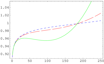
(a)                                                             (b)

Figure 1: $V/V_{0}$ as a function of $x=\varphi/\varphi_{1}$. In figure (a) the curves correspond to parameter choices with $\mathcal{B}>1$ (upper, green), $\mathcal{B}=1$ (middle, red), and $\mathcal{B}<1$ (lower, blue). Figure (b) is for $\alpha\xi=1$.

Before delving into the details of the inflationary dynamics, we will discuss some general properties of the inflaton potential (4.14). At $\varphi=\varphi_{c}$ one of the waterfall fields becomes tachyonic, triggering the symmetry breaking phase transition ending inflation. If $V^{\prime}(\varphi_{c})<0$, as in figure 1b, the inflaton will never reach this value. Instead it will end up in the wrong vacuum at the minimum of $V_{\rm inf}$ occurring at $\varphi\gg\varphi_{c}$. In the $\xi\ll 1$ limit

$$V^{\prime}(\varphi_{c}) =\frac{g^{2}\lambda^{2}\xi\varphi_{c}}{8\pi^{2}}\left\{\ln 2\sqrt{1+\frac{\alpha^{2}\xi^{2}}{9}}+\frac{\alpha\xi}{3}\left[\frac{1}{2}+\mathrm{arcsinh}\,\frac{\alpha\xi}{3}+\ln\frac{4g^{2}\xi}{Q^{2}}\right]+\Or(\xi)\right\}$$ (4.20)

$$=\frac{g^{2}\lambda^{2}\xi\varphi_{c}}{8\pi^{2}}\left\{\ln 2+\frac{\alpha\xi}{3}\left[\ln\frac{g^{2}\xi}{Q^{2}}+\frac{1}{2}+2\ln 2\right]+\Or(\xi,\alpha^{2}\xi^{2})\right\}\,.$$

which becomes negative for larger values of $\alpha\xi$. Requiring $V^{\prime}(\varphi_{c})>0$, to ensure that the system ends up in the right vacuum, therefore gives us an upper bound on $\alpha$. For example if $g^{2}\xi/Q^{2}=10^{-6}$ then $\alpha\xi\lesssim 0.175$ is the required bound. Recall that $\alpha$ parametrises the ratio of the moduli to inflationary scale (3.16, 3.18), which should be larger than unity to keep the moduli fields stabilised during inflation. Successful inflation with the moduli stabilised, and with the inflaton ending up at the critical value $\varphi_{c}$, is possible when (in the $\xi\ll 1$ limit)

$$1\lesssim\alpha\lesssim\frac{3\ln 2}{\xi\ln(Q^{2}/[g^{2}\xi])}\,.$$ (4.21)

The critical value of $\varphi$ at which inflation ends is then

$$\varphi_{c}=\frac{g\sqrt{2\xi}}{\lambda}[1+\Or(\alpha\xi)]\,.$$ (4.22)

In terms of the gaugino condensation parameters of the $SU(N)$ group in (2.9), $\alpha$ in the above range requires $24\leq N\leq 250$, for $g^{2}=0.1$, $\xi=10^{-5}$. This is a wide range of acceptable $N$, though large gauge groups are needed. For smaller $N$ the combination $\alpha\xi$ is too large.

The inflaton potential features minima and maxima (see figure 1a). To better understand their occurrence, we perform a $\varphi\gg\varphi_{1}$ asymptotic expansion. Taking $\xi\ll 1$ (as implied by the COBE bound (5.3)), the asymptotic inflationary potential reduces to

$$V_{\rm inf}\approx\frac{g^{2}\xi^{2}}{2}\left\{1+\frac{g^{2}}{8\pi^{2}}\ln\frac{\lambda^{2}\varphi^{2}}{2Q^{2}e^{-3/2}}+\frac{\lambda^{2}\varphi^{2}}{24\pi^{2}}\left[(\alpha+1)\ln\frac{\lambda^{2}\varphi^{2}}{2Q^{2}e^{-3/2}}-1\right]\right\}\,,$$ (4.23)

with the next higher order corrections being $\Or(\varphi_{1}^{2}/\varphi^{2})$. The above limit would not be valid if $\alpha\xi\gg 1$, but we already know this can not be the case from (4.21) above. We see that the slope of the above potential is sensitive to the choice of cutoff scale $Q$, in contrast to SUSY hybrid inflation models. The corrections to $n_{s}$ from the moduli sector are also strongly dependent on $Q$. Before precise predictions are extracted from the model, $Q$ needs to be absorbed into the other parameters by renormalisation. This will not be covered here. We expect the errors to be minimised by taking the renormalisation scale to be of order $\lambda\varphi_{*}$.

In usual $D$-term hybrid inflation $V$ is monotonic. However because of the $\varphi^{2}\ln\varphi^{2}$ correction from the coupling to the moduli sector, this is no longer true. To find the extrema, we calculate the derivative of the above asymptotic potential (4.23)

$$V^{\prime}_{\rm inf}\approx\frac{g^{4}\xi^{2}}{8\pi^{2}}\frac{1}{\varphi}\left[1+\frac{\varphi^{2}}{\mathcal{B}\varphi_{x}^{2}}\left(\ln\frac{\varphi^{2}}{\varphi_{x}^{2}}-1\right)\right]\,,$$ (4.24)

where

$$\varphi_{x}^{2}=\frac{2Q^{2}}{e^{5/2}\lambda^{2}}e^{1/(\alpha+1)}\,,\qquad\mathcal{B}=\frac{3g^{2}}{\lambda^{2}(1+\alpha)\varphi_{x}^{2}}\,.$$ (4.25)

Hence $V^{\prime}=0$ whenever $-\varphi^{2}\ln[{\varphi^{2}}/({e\varphi_{x}^{2}})]=\mathcal{B}\varphi_{x}^{2}$. If $\mathcal{B}$ is small this equation has two solutions and the potential has a maximum and a minimum, with $0<\varphi_{\rm max}<\varphi_{x}<\varphi_{\rm min}$. This is true up until the critical value $\mathcal{B}=1$, where the two extrema merge at $\varphi=\varphi_{x}$. For larger $\mathcal{B}$ the slope of the potential is never zero. This is illustrated in figure 1a, which shows $V$ for various choices of $\mathcal{B}$.

The value of $\mathcal{B}$ depends on $\alpha$, which is sensitive to the details of the moduli sector. Since $\alpha\geq 0$ we find an upper bound of

$$\mathcal{B}=\frac{3g^{2}e^{5/2}}{2Q^{2}(1+\alpha)e^{1/(1+\alpha)}}\lesssim 18.3\,\frac{g^{2}}{Q^{2}}\,.$$ (4.26)

If the moduli sector has the form described in subsection 2.2.1, then we can use the approximate expression (3.18) for $\alpha$. Assuming $\alpha\gg 1$, we obtain

$$\mathcal{B}\approx 27.4\,\frac{g^{4}\xi^{2}}{Q^{2}m_{3/2}^{2}}\,,$$ (4.27)

so in this case we usually have $\mathcal{B}\ll 1$. More generally, we expect $g$ to be small and $\alpha$ to be large, so the maximum (and minimum) are typically present. For the limiting case $\mathcal{B}\ll 1$, or equivalently $(1+\alpha)\gg g^{2}$, we find

$$\varphi^{2}_{\rm max}\approx\frac{3g^{2}}{\lambda^{2}(1+\alpha)\ln(e/\mathcal{B})}\,.$$ (4.28)

The presence of the maximum is solely due to the coupling to the moduli sector. If the initial value of the inflaton is larger that $\varphi_{\rm max}$, it will roll to the minimum of $V_{\rm inf}$ and inflation will never end. To avoid this we must either have $\mathcal{B}\geq 1$ or tune the initial conditions for inflation. This initial value problem will be most severe for models where inflation needs to take place close to the maximum.

5 Slow-Roll Inflation

5.1 Matching with observations

In the previous section we derived the inflationary potential for our model, including the one-loop effects. The parameters appearing in this potential are constrained by the data, since the density perturbations produced should match the observed ones.

We recall here the important formulae for the density perturbations. Observable scales leave the horizon $N_{*}\approx 60$ $e$-folds before the end of inflation, with

$$N(\varphi)\approx\int^{\varphi}_{\varphi_{\rm end}}\frac{V}{V^{\prime}}{\rm d}\varphi,$$ (5.1)

in the slow-roll approximation. Here $\varphi_{\rm end}$ is the value of $\varphi$ when inflation ends, which is either the critical value $\varphi_{c}$ where one of the waterfall fields becomes tachyonic, or the value for which one of the slow roll parameters exceeds unity. The slow roll parameters are defined as

$$\eta=\frac{V^{\prime\prime}}{V}\,,\qquad\epsilon=\frac{V^{\prime 2}}{2V^{2}}$$ (5.2)

and $V\approx V_{0}$ during inflation. The amplitude of the perturbations is

$$\delta_{H}=\frac{1}{5\sqrt{3}\pi}\frac{V^{3/2}}{V^{\prime}}\Big{|}_{\varphi=\varphi_{*}}$$ (5.3)

where $\varphi_{*}$ is the value of the inflaton $N_{*}$ $e$-folds before the end of inflation. This should match the COBE normalisation $\delta_{H}\approx 1.91\times 10^{-5}$ [14, 37]. The spectral index

$$n_{s}=1+2\eta-6\epsilon\,$$ (5.4)

is also constrained by the data. Although the precise observed value of $n_{s}$ is sensitive to the choice of prior, it will be in the range $0.9\lesssim n_{s}\lesssim 1$. In hybrid inflation the second slow-roll parameter $\epsilon$ is usually very small, which implies a negligible tensor-to-scalar ratio $r=12.8\epsilon$. In this case, the WMAP 3-year data prefer smaller values for the spectral index: $n_{s}=0.951^{+0.015}_{-0.019}$ [20].

The formation of cosmic strings at the end of hybrid inflation gives additional constraints on the theory, since the string tension $\mu$ is constrained by the data. Strings can contribute a few percent to the density perturbations, which bounds $G\mu\lesssim 3\times 10^{-7}$ [23, 24]. The non-observation of irregularities in pulsar timing experiments bounds the stochastic gravitational wave background produced by strings, which can be translated into the bound $G\mu\lesssim 1\times 10^{-7}$ [38, 39, 40]. The mass-per-unit length of a SUSY $D$-term string is directly related to the Fayet-Iliopoulos term by $\mu=2\pi\xi$ [21]. The presence of the extra moduli fields will give corrections to this, which could help satisfy the constraints on $\mu$.

5.1.1 Small corrections to SUSY hybrid inflation

We will begin by determining for which parameter ranges the moduli corrections are small, and our SUGRA model behaves in a similar way to the corresponding SUSY model. As is usually done with SUSY hybrid inflation, we will consider two limiting possibilities for the ratio $\varphi_{*}/\varphi_{c}$. Recall that $\varphi_{*}$ is the value of $\varphi$ when the density perturbations are produced, and $\varphi_{c}$ is its value when inflation ends.

In the limit that $\varphi_{*}\gg\varphi_{c}$, we can use the asymptotic form of the inflaton potential (4.23). As we will see, this is a good approximation for superpotential couplings which are not excessively small $\lambda\gtrsim 10^{-5}$. In this limit (5.1) can be written as

$$\frac{g^{2}}{2\pi^{2}}\frac{dN}{d\varphi^{2}}=\left[1+\frac{\varphi^{2}}{\mathcal{B}\varphi_{x}^{2}}\ln\frac{\varphi^{2}}{e\varphi_{x}^{2}}\right]^{-1}\,.$$ (5.5)

The effects of the moduli corrections will be small when $\varphi^{2}\ll\mathcal{B}\varphi_{x}^{2}=3g^{2}/[\lambda^{2}(1+\alpha)]$. In this limit, the right hand side of equation (5.5) is approximately 1 throughout inflation. Taking the first order moduli corrections into account, we find

$$\frac{g^{2}N}{2\pi^{2}}=\varphi^{2}+\frac{\varphi^{4}}{4\mathcal{B}\varphi_{x}^{2}}\left(3-2\ln\frac{\varphi^{2}}{\varphi_{x}^{2}}\right)+\Or\left(\frac{\varphi^{6}}{\mathcal{B}^{2}\varphi_{x}^{6}}\right)\,.$$ (5.6)

Inverting the above expression, and changing to the usual inflationary parameters, then gives

$$\varphi_{*}^{2}\approx\frac{g^{2}N_{*}}{2\pi^{2}}\left[1+\frac{\lambda^{2}(1+\alpha)N_{*}}{12\pi^{2}}\left\{2-\frac{1}{1+\alpha}+\ln\frac{N_{*}g^{2}\lambda^{2}}{4\pi^{2}Q^{2}}\right\}\right]\,.$$ (5.7)

When $g^{2}\lambda^{2}/Q^{2}\lesssim 0.1$, the moduli corrections make the potential less steep, and reduce the value of $\varphi_{*}$ with respect to the standard SUSY result $\varphi_{*}^{2}=g^{2}N/(2\pi^{2})$. Just as in SUSY hybrid inflation the first slow roll parameter $\epsilon\ll\eta$ is small; the spectral index becomes

$$n_{s}\approx 1+2\eta\approx 1-\frac{1}{N_{*}}+\frac{\lambda^{2}(1+\alpha)}{4\pi^{2}}\left\{\frac{11}{3}-\frac{1}{1+\alpha}+\ln\frac{N_{*}g^{2}\lambda^{2}}{4\pi^{2}Q^{2}}\right\}\,.$$ (5.8)

The SUSY result for the spectral index is $n_{s}\approx 1+2\eta\approx 1-1/N_{*}\approx 0.98$. For $g^{2}\lambda^{2}/Q^{2}\gtrsim 0.1$ the moduli corrections increase this value. In the opposite limit $g^{2}\lambda^{2}/Q^{2}\lesssim 0.1$, the spectral index is reduced and can match the best fit WMAP3 value $n_{s}=0.95$. However, this requires the moduli corrections to be substantial, and the result is sensitive to the details of renormalisation.

The amplitude of the density perturbations should match the COBE result. This fixes the FI-term

$$\xi=\frac{5\sqrt{3}\delta_{H}}{2\sqrt{N_{*}}}\left[1+\frac{\lambda^{2}(1+\alpha)N_{*}}{8\pi^{2}}\left\{\frac{8}{3}-\frac{1}{1+\alpha}+\ln\frac{N_{*}g^{2}\lambda^{2}}{4\pi^{2}Q^{2}}\right\}\right]$$ (5.9)

and gives $\xi\sim 10^{-5}$ as usual.

The large-$\varphi$ asymptotic expansion that we have used in the above analysis is only valid if $\varphi_{*}\gg\varphi_{c}$ which implies $\lambda^{2}\gg\xi\sim 10^{-5}$. For smaller couplings the full potential should be taken into account; this limit is discussed below, at the end of the subsection. The power series expansion used to derive (5.6) is valid if $\lambda^{2}(1+\alpha)$ is small, so that the moduli corrections are subdominant. In general this is also the condition for $n_{s}$ to be compatible with WMAP (an exception to this is discussed in subsection 5.2.2). Using (5.8), and (3.18), we see that if our model is to have any hope of compatibility with the CMB, it must satisfy

$$10^{-5}\ll\lambda^{2}\lesssim\frac{1}{\alpha|\ln\lambda^{2}g^{2}/Q^{2}|}\sim\frac{V_{0}}{m_{3/2}^{2}|\ln\lambda^{2}g^{2}/Q^{2}|}\,.$$ (5.10)

We note that this is also consistent with $\alpha\xi$ being small, as is required for inflation to end in the right vacuum (4.21). In contrast to $\lambda$, the gauge coupling $g$ is not strongly constrained. This is not true for string motivated models for which the Bogomolnyi bound applies, since $g\sim\lambda$. Substituting this, and the definition of $V_{0}$, in to the above constraint, we obtain

$$m_{3/2}\lesssim\xi\,.$$ (5.11)

Since $\xi\sim 10^{-5}$, this places a strong restriction on $m_{3/2}$, which is equal to the moduli stabilisation scale for the model we are studying. This implies that the inflation and moduli scales must be dangerously close, unless the gauge coupling $g$ is very small. This raises questions about the viability of such string motivated inflation models. Even if $g$ is small, the above bound will impose a strong restriction on the moduli sector. For the example described by (2.9), we find that $N>206$ is needed to satisfy the bound. However it should be noted that our moduli stabilisation sector can hardly be described as generic, so perhaps the problem can be evaded without changing the inflation sector significantly.

The usual treatment of hybrid inflation in a stringy context is to assume the moduli are fixed at some high scale, and then to neglect their presence during inflation. We see from (5.10) that this is only a good approximation for a limited range of the superpotential coupling $\lambda$. Paradoxically enough, the larger the modulus scale and thus the better fixed the moduli are, the less their presence can be ignored, and the stronger the bound on $\lambda$ is. For larger couplings the moduli corrections dominate, generically resulting in a spectral index at odds with the WMAP result.

The above analysis using the asymptotic approximation (5.5) will not be valid if inflation takes place close to the critical point $\varphi_{*}\approx\varphi_{c}$. We will now study this limiting case, which will apply for small coupling $\lambda^{2}\lesssim 10^{-5}$. The modulus corrections are small if $\lambda^{2}(1+\alpha)\ll 1$, which is automatic in this regime (it follows from $\alpha\xi\lesssim 0.1$, see (4.21), together with $\xi\lesssim 10^{-5}$). Hence, the usual SUSY results are recovered. In particular, in the limit $\varphi_{*}\to\varphi_{c}$ we find

$$\xi \approx 10^{-5}\left(\frac{\lambda^{2}}{10^{-5}}\right)^{1/3}$$ (5.12)

$$n_{s} \approx 1+2\eta\approx 1+\frac{(\varphi_{*}/\varphi_{c}-1)}{8\pi^{2}}\ln(\varphi_{*}/\varphi_{c}-1)\approx 1\,.$$ (5.13)

The FI-term $\xi$ scales with $\lambda^{2/3}$ and can be made arbitrary small for arbitrary small coupling. However, in the small coupling regime the perturbation spectrum is indistinguishable from a scale invariant spectrum, which is disfavoured by the latest WMAP results.

5.2 Large deviations from SUSY hybrid inflation

We will now consider regions of parameter space in which the influence of the moduli sector is significant. Typically this gives unacceptably large corrections to $n_{s}$, allowing the corresponding parameters to be ruled out.

As was shown in the previous section, if $\varphi_{*}$ is close $\varphi_{c}$, then moduli corrections must always be small. Therefore we can take the $\varphi_{*}\gg\varphi_{c}$ limit throughout this subsection, and use the asymptotic expression (5.5) to find the behaviour of the inflaton. Note that it is still possible to get $N_{*}\sim 60$ $e$-folds of inflation no matter the value of $\mathcal{B}$. If $\mathcal{B}\geq 1$, the potential has no maximum and $N$ can be made arbitrary large by taking the initial value of $\varphi$ arbitrary larger. Alternatively if $\mathcal{B}<1$ tuning $\varphi$ to start sufficiently close to the maximum increases $N$.

The equation (5.5) can be analysed numerically, as we will show in the next subsection. Although we cannot find analytic solutions to it, we can find approximate analytic expressions in the limiting cases of $\mathcal{B}\approx 1$ and $\mathcal{B}\ll 1$, which are covered in subsections 5.2.2 and 5.2.3 respectively. These results help us understand the parameter dependence of the corrections to $n_{s}$. It should be noted that the value of $n_{s}$ in these regimes is very sensitive to the effects of the moduli sector. The renormalisation of the theory also needs to be dealt with. For the model to be compatible with WMAP in these cases, significant fine-tuning of the physics above the inflationary scale is required.

5.2.1 Numerical analysis

Introducing the notation

$$u=\frac{g^{2}N}{2\pi^{2}\varphi_{x}^{2}\mathcal{B}}=\frac{\lambda^{2}(1+\alpha)}{6\pi^{2}}N\,,\qquad Y=\frac{\varphi^{2}}{e\varphi_{x}^{2}}\,,$$ (5.14)

with $\varphi_{x}$ and $\mathcal{B}$ given in (4.25), equation (5.5) above can be brought into the form

$$\frac{dY}{du}=\frac{\mathcal{B}}{e}+Y\ln Y\,.$$ (5.15)

The first term on the right is the usual $D$-term inflation potential, whereas the $Y\ln Y$ term encodes the contribution from the moduli sector. If this sector was absent the solution of the above equation would reduce to $\mathcal{B}u=eY$. In the $\varphi\gg\varphi_{c}$ asymptotic limit we are considering, $\eta\gg\epsilon$, and the expression for the spectral index (5.4) reduces to

$$n_{s}\approx 1+2\eta\approx 1-\frac{u}{N_{*}eY}\left(\mathcal{B}-eY[2+\ln Y]\right)\,.$$ (5.16)

The COBE constraint (5.3) on the power spectrum becomes

$$\xi=\frac{5\sqrt{3}\delta_{H}}{2\sqrt{N_{*}}}(\mathcal{B}+eY\ln Y)\left(\frac{u}{e\mathcal{B}Y}\right)^{1/2}\,.$$ (5.17)

If we take the limit $Y,u\to 0$ with $u\mathcal{B}/Y\to e$ in the above expressions, they reduce to the standard SUSY hybrid inflation results.

Having determined $Y$ numerically with (5.15), we see that the spectral index $n_{s}$, and also $\xi$, depend only on the parameter combinations $u$ and $\mathcal{B}$. The variation of $n_{s}$ in terms of these parameters is plotted in figure 2. We see that $n_{s}$ is compatible with WMAP only if $u$ is small or if $\mathcal{B}$ is close to its critical value of one. The limit of small $u$, or equivalently small $\lambda^{2}(1+\alpha)$, corresponds to the corrections from the moduli sector being subdominant. This region of parameter space was covered analytically in subsection 5.1.1. For other parameter choices the moduli corrections are significant. As we see from figure 2, this usually leads to an unacceptable value of $n_{s}$. An exception to this is when $B\approx 1$, where the different corrections to $n_{s}$ cancel. This case is analysed in subsection 5.2.2. For large $\alpha$, which is the most realistic situation, $\mathcal{B}$ is small, and only the lower part of figure 2 is relevant. An acceptable spectral index typically requires $u$ small, which occurs when $\lambda$ is small. This case is discussed in subsection 5.2.3.

We note that since $u$ is proportional to $\lambda^{2}$ and $\mathcal{B}$ to $g^{2}$ the $\lambda=\sqrt{2}g$ Bogomolnyi limit is contained in figure 2 as a $45^{\circ}$ straight line. The position of the line depends on $\alpha$. For large $\alpha$, suitable $n_{s}$ will only be obtained if $\lambda$ is very small or if $\mathcal{B}$ is fine-tuned to be close to 1. This can place strong restrictions on the string theory motivated inflation models for which this limit applies.

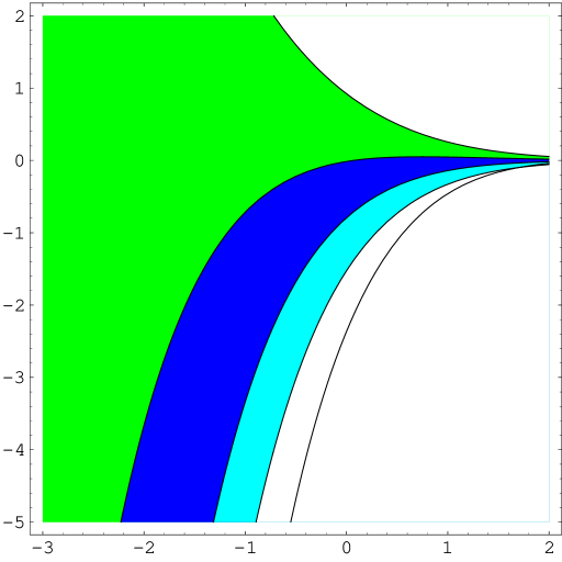
Figure 2: Contour plot of $n_{s}$ for $\ln\mathcal{B}$ vs. $\ln u$. The upper contour is $n_{s}=1$, and the lower one is $n_{s}=0.9$. The 1-$\sigma$ WMAP3 results correspond to the dark (blue) region in between. Parameters to the right of the black line below the contours satisfy the cosmic string bound on $\xi$.

The value of $\xi$ required to satisfy the COBE bound can also be found in terms of $u$ and $\mathcal{B}$. For the parameter choices which give an acceptable value of $n_{s}$, we find $\xi$ in the range $10^{-5}$–$10^{-6}$, so the moduli corrections do not change it significantly. In particular we find that we cannot simultaneously pull $\xi$ down to a value which will give a sufficiently low value of the string tension $\mu$, and also keep $n_{s}$ in the acceptable range. This can been seen from figure 2, where the cosmic string bound on $\xi$ is represented by the black line. Hence some other mechanism will be required to reduce the cosmic string contribution to the CMB.

5.2.2 Approximation for $\mathcal{B}\approx 1$

There is one regime where the moduli corrections can dominate, and yet the spectral index remains in agreement with the data. This is when $\mathcal{B}\approx 1$, i.e. close to the critical value where the maximum in the potential disappears. To see how this comes about it would be useful to have an analytic expression which covers this region, but unfortunately we do not have an analytic solution for the integral (5.5). However, it can be evaluated if we take

$$-\frac{\varphi^{2}}{\varphi_{x}^{2}}\ln\frac{\varphi^{2}}{e\varphi_{x}^{2}}\approx\left(2-\frac{\varphi^{2}}{\varphi_{x}^{2}}\right)\frac{\varphi^{2}}{\varphi_{x}^{2}}$$ (5.18)

which is a reasonable approximation in the region $\varphi^{2}/\varphi_{x}^{2}\lesssim e$. Inflation in the small $\lambda^{2}(1+\alpha)$ regime has already been covered in subsection 5.1.1. Here we will take the $\lambda^{2}(1+\alpha)\gg 1$ limit, which will only realistically occur when $\alpha\gg 1$ (since $\lambda\lesssim 1$).

In addition to the limit $\lambda^{2}\alpha\gg 1$, we also take $|\mathcal{B}-1|\ll 1$, since our numerical analysis tells us that these are the only values of $\mathcal{B}$ which will give a sensible value for $n_{s}$. The approximate inflaton solution for these limits is

$$\frac{\varphi^{2}}{\varphi_{x}^{2}}\approx 1-\frac{6\pi^{2}N}{\lambda^{2}\alpha}+\left[\frac{\lambda^{2}\alpha}{18\pi^{2}N}+\frac{1}{3}\right](\mathcal{B}-1)+\cdots\,.$$ (5.19)

Substituting this into the expression (5.16) for the spectral index (and using the above approximation for $\varphi^{2}\ln\varphi/\varphi_{x}$) gives

$$n_{s}\approx 1-\frac{2}{N_{*}}\left[1+\frac{3\pi^{2}N_{*}}{\lambda^{2}\alpha}\right]+\frac{\lambda^{4}\alpha^{2}(\mathcal{B}-1)}{54\pi^{4}N_{*}^{3}}\left[1+\frac{3\pi^{2}N_{*}}{\lambda^{2}\alpha}\right]$$

$${}+\Or\left(\frac{1}{\lambda^{4}\alpha^{2}},\mathcal{B}-1,\lambda^{8}\alpha^{4}[\mathcal{B}-1]^{2}\right)\,.$$ (5.20)

So if we keep $\lambda^{4}\alpha^{2}|\mathcal{B}-1|\lesssim 1$, the spectral index $n_{s}$ will remain in the acceptable range. This is in qualitative agreement with our numerical analysis. However it should be noted that $\mathcal{B}\sim g^{2}/[\alpha Q^{2}]$, so if $\alpha$ is too large, then (since $g\lesssim 1$) it will not be possible to have $\mathcal{B}\approx 1$. The solution in this regime is extremely sensitive to the moduli effects, and so its viability requires fine-tuning of the high energy physics at the moduli stabilisation scale. On a more positive note, we see from (4.26) that if $\alpha\lesssim 18$, then it is still possible to obtain agreement with the WMAP data even when $g,\lambda\sim 1$. Hence it may be possible for the Bogomolnyi limit to apply without a very small value of $g$ being required.

5.2.3 Low $\varphi$ maximum ($\mathcal{B}\ll 1$)

There is one other physically interesting region of parameter space for which we can determine the approximate analytic behaviour of the inflaton. We will consider the limiting case where $V$ has a maximum which occurs at a value of $\varphi$ which is far lower than $\varphi_{x}$. This case corresponds to the $\mathcal{B}\ll 1$ limit. Since we naturally expect $\alpha$ to be large, and $\mathcal{B}\sim 1/\alpha$, the above limit will frequently be satisfied.

When the potential (4.23) has a maximum (i.e. if $\mathcal{B}\leq 1$), we can rewrite the equation (5.5) as

$$\frac{g^{2}}{2\pi^{2}}\frac{dN}{d\varphi^{2}}=\left[1-\frac{\varphi^{2}}{\varphi_{\rm max}^{2}}-\frac{\varphi^{2}}{\varphi_{\rm max}^{2}}\frac{\ln(\varphi^{2}/\varphi_{\rm max}^{2})}{\ln(e\varphi_{x}^{2}/\varphi_{\rm max}^{2})}\right]^{-1}\,.$$ (5.21)

The magnitude of the third term in the bracket is bounded by $[e\ln(e\varphi_{x}^{2}/\varphi_{\rm max}^{2})]^{-1}$, so if $\varphi_{x}\gg\varphi_{\rm max}$, as is the case for small $\mathcal{B}$, we can neglect it to leading order. We then obtain the approximate solution

$$\varphi^{2}\approx\varphi_{\rm max}^{2}+\left(\varphi_{c}^{2}-\varphi_{\rm max}^{2}\right)\exp\left(-\frac{g^{2}N}{2\pi^{2}\varphi_{\rm max}^{2}}\right)$$ (5.22)

which is valid throughout inflation. The usual SUSY result is obtained in the limit $g^{2}N/(2\pi^{2}),\varphi_{c}^{2}\ll\varphi_{\rm max}^{2}$.

Taking $\varphi\gg\varphi_{c}$, and assuming $\epsilon\ll\eta$, we find

$$n_{s}\approx 1+2\eta\approx 1-\frac{g^{2}}{2\pi^{2}\varphi_{\rm max}^{2}}\left\{\left[1-\exp\left(-\frac{g^{2}N_{*}}{2\pi^{2}\varphi_{\rm max}^{2}}\right)\right]^{-1}+1\right\}\,.$$ (5.23)

We see that reducing $\varphi_{\rm max}/g$ pushes $n_{s}$ down, away from the usual SUSY result. If $\varphi_{*}$ is too close to the maximum, $n_{s}$ will be too low. This allows us to bound the parameters of the moduli sector. For sensible values of $n_{s}$, we need $g^{2}N_{*}/[2\pi^{2}\varphi_{\rm max}^{2}]$ to be small. If $\mathcal{B}$ is small, we can use the approximate expression (4.28) for $\varphi_{\rm max}$. For $\alpha\gg 1$, this implies the bound

$$\lambda^{2}\lesssim\frac{1}{\alpha\ln(\alpha Q^{2}/g^{2})}\,,$$ (5.24)

which is similar to the bound derived in subsection 5.1.1. Again, these results are applicable in the Bogomolnyi limit.

We also find that the value of $\xi$ implied by the COBE constraint decreases when $\varphi_{\rm max}/g$ is reduced. This suggests that if the moduli corrections are large enough, the cosmic string bound on $\xi$ could be satisfied. However if we use the above bound on $\varphi_{\rm max}/g$ from the spectral index constraint, we find that we must have $\xi\gtrsim 10^{-6}$, which does not satisfy the cosmic string bound.

6 Cosmic strings

In our model of $D$-term inflation coupled to moduli, cosmic strings form during the breaking of the Abelian gauge symmetry $U(1)_{1}$ by the waterfall field $\phi^{+}$ at the end of inflation. The cosmic strings in our model are not BPS as in usual $D$-term inflation. This is due to the non-vanishing of the gravitino mass and the coupling of the string fields to the moduli sector. Non-observation of cosmic strings constrains the string tension. To see what this implies for the parameters in our model, we will study the string solution and the fermionic zero modes.

The cosmic string solution has the form

$$\phi^{+}=[(2T_{\rm R}-|\chi|^{2})\xi]^{1/2}e^{in\theta}f(r)\,,\qquad\phi^{-}=\phi=0\,,\qquad A_{\theta}=na(r)$$ (6.1)

and the moduli sector fields depend only on $r$. The functions $f(r)$, $a(r)$, are similar to the standard ones appearing in the Abelian string model [39]. The Higgs field tends to its vacuum value at infinity, and regularity implies it is zero at the string core. Without loss of generality we can take the winding number positive $n>0$. If the variation of the moduli fields inside the string is small, the string solution will be similar to a BPS $D$-string, with a similar string tension, which (for $n=1$) is

$$\mu\approx 2\pi\xi\,.$$ (6.2)

The above result will receive corrections from the one loop contribution to the potential. We also expect that the variation of the moduli fields inside the string will reduce $\mu$ (recall that $\xi=\xi(T,\chi)$, so $\xi$ could be reduced inside the string core). Throughout this paper we have assumed that the moduli are stabilised by a very steep potential, which is not significantly changed by any inflation scale contributions. The cosmic strings have the same energy scale as inflation so, for the parameters we have considered, we expect the above result to hold. It should also be noted that an important ingredient in the determination of the tension is the width of the Higgs profile, which is set by the inverse Higgs mass. Although supersymmetry is broken in the vacuum, the Higgs mass does not receive a soft mass contribution. This is due to our choice of Kähler potential, with the Higgs field inside the logarithm (3.13).

The string tension is constrained by the data: CMB and pulsar timing experiments give a comparable bound $G\mu\lesssim 10^{-7}$ [23, 38, 39]. This translates in a tight constraint on the effective FI parameter $\xi$. As discussed in section 5, $\xi$ determines the size of the density perturbations produced and is thus fixed by the CMB data. In most of parameter space $\xi\approx 10^{-5}$ needed, in conflict with the cosmic string bound. The only exception is for very small superpotential couplings $\lambda^{2}\lesssim 10^{-9}$, but at the cost of having a slightly disfavoured spectral index $n_{s}=1$ (5.12, 5.13). It is interesting to note that the string contribution can be small even when the gauge coupling constant $g$ is large, this is because we are using a shift symmetry for the inflaton. This is in sharp contrast to standard $D$-term inflation which uses a minimal Kähler potential for the inflaton. Another, more attractive, way to evade the cosmic string bound has been proposed in [26]. If the model is augmented by a second set of Higgs fields, which are put in a global $SU(2)$ multiplet together with the original Higgs fields, the strings formed at the end of inflation are semi-local [27]. In the language of brane inflation this requires an additional D7 brane [8]. Semi-local strings are not topologically stable, and they ultimately decay, thereby easing the cosmic string bound.

Even if the string bound is somehow evaded, there are also constraints arising from vorton bounds [29, 30], although these are very model dependent [41]. If a fermion couples to a string Higgs field, the string can act as a potential well, and zero mode fermion bound states can exist on it. Excitation of these will produce currents [42]. If the currents are stable and their generation is not suppressed the vortons will be stable and will soon dominate the energy density of the universe. This potentially constrains any model with fermion zero modes.

Since our model is supersymmetric, it will inevitably contain a large number of fermion fields which provide candidates for zero mode bound states [22]. Given the potentially serious implications arising from them, it is important to determine the number of zero modes. The number of zero mode solutions is given by an index theorem, and depends only on the charges of the fermion under the string generator (in our model the generator of the $U(1)_{1}$ symmetry) and the string winding number [43, 44]. Applying the theorem to the $\tilde{\phi}$-$\tilde{\phi}^{-}$ sector (which decouples from the other fermion fields), we find [28]

$$N^{-}=2n$$ (6.3)

negative chirality real zero modes (or equivalently $n$ complex ones). There are $N^{+}=0$ positive chirality ones in this sector.

The other fermion fields couple to the gravitino, which complicates things. Firstly, gravitinos are gauge fields, so it is necessary to fix the gauge before analysing the system. In [44] the $\bar{\sigma}^{\mu}\psi_{\mu}=0$ gauge was used. This leaves three degrees of freedom, which were denoted $\Psi$, $\Sigma$ and $\Pi$ in that paper. Another complication arises from the fact that gravitinos have different kinetic terms to the other fermions. Nevertheless an index theorem can be derived [44]. Applying it to our model gives $N^{+}=2(n+1)$, and $N^{-}=0$. However this result should be treated with caution. The fermion norm obtained for the above gauge choice does not appear to be positive definite, and so some of these apparent zero mode solutions may be gauge. We conjecture that one complex zero mode is due to a residual unbroken supersymmetry or Lorentz transformation, and that the field $\Pi$ (see [44]) should be ignored. We then find

$$N^{+}=2n\,.$$ (6.4)

Hence we find that there are equal numbers of positive and negative chirality zero modes. Since the direction of the corresponding massless states is determined by their chirality, we see there are equal number of left and right movers on the string. This could lead to a smaller net current and hence weaker bounds on the model.

It is interesting to contrast the above results with those for $D$-term inflation without a moduli sector. The number of negative chirality zero modes is unchanged (irrespective of whether the model is SUSY or SUGRA). In a SUSY model the number of positive chirality modes is $2n$ [22], just like (6.4). However when the gravitinos are included (which will be massless when the moduli sector is absent), they mix with one pair of zero modes and it is no longer a bound state [28], so $N^{+}$ is reduced to $2(n-1)$ [44]. Hence for a winding number $n=1$ string, all zero modes move in the same direction and the current will be maximal (and the bounds stronger) [45]. On the other hand, for the model described in this paper, the introduction of the moduli sector gives a non-zero gravitino mass. This helps relocalise the zero mode, and the resulting currents are no longer chiral.

If vortons do arise in our model then the string tension will be constrained since vortons are long lived. There are two constraints one can apply [29, 30]. Firstly, and more conservatively, the universe should be radiation dominated at nucleosynthesis. Consequently, this constrains the string tension such that $G\mu\lesssim 10^{-20}$. Alternatively if the vortons are very long lived then we require them not to overclose the universe, in which case $G\mu\lesssim 10^{-24}$. These constraints are much stronger than the current bounds on cosmic $D$-strings in brane inflation models, but are not as strong as those cited in [45] where only BPS strings were considered. A possible way around this is for there to be a low reheat temperature. In this case we could envisage the possibility of $D$-loop dark matter. We note that semi-local strings are likely to evade these bounds since they are probably not stable enough for vorton formation.

7 Conclusions

Hybrid inflation can be realised in supergravity as the low energy description of string systems such as the D3/D7 brane configurations. At tree level the inflation potential is flat, only lifted by loop corrections leading to a slow rolling inflationary phase. However it must not be forgotten that in the full underlying theory, there will be other non-inflationary fields, which could interfere with slow-roll. In particular, moduli fields are pervasive in most string compactifications. If not stabilised, these lead to flat directions at the perturbative level. This poses a serious problem for any attempt to embed inflationary cosmology within string theory. Even if the moduli are stabilised, the stabilisation mechanism itself can damage the flatness of the inflationary potential.

In this paper we have analysed a combined SUGRA model of $D$-term hybrid inflation and stabilised moduli. The inclusion of moduli requires substantial changes to most aspects of the inflation model. First of all, it is difficult to use a constant Fayet-Iliopoulos term to give the inflation vacuum energy when other sectors are present in the theory. Instead, we have shown how an effective FI-term can be obtained from the VEVs of stabilised moduli fields. The moduli sector we took has an additional Abelian gauge symmetry. For suitable moduli charges, the resulting $D$-term is positive definite. This second $D$-term allows one to obtain an effective Fayet-Iliopoulos term, whose presence is required to lift the AdS vacuum in the moduli sector to a Minkowski one. By coupling the moduli fields to the inflationary $U(1)$, this effective Fayet-Iliopoulos term can also be made to appear in the inflationary $D$-term, making inflation possible.

The inclusion of the moduli sector also has implications for the choice of Kähler potential. Using a minimal Kähler potential for the inflationary sector results in a large mass for the inflaton field, destroying the flatness of the potential. In other words, the presence of the moduli sector causes the well-known $\eta$-problem to appear in $D$-term inflation. The problem can be cured by introducing a shift symmetry for the inflaton field in the Kähler potential. The inflaton potential is then obtained at the one loop level, but receives drastic modifications due to the coupling to moduli. The requirement that inflation ends normally imposes further restrictions on the full Kähler potential. Taking it to be of the no-scale form (3.13) gives a working model. The variation of moduli fields during inflation is another potential source of problems, although for our $D$-term model they can easily be avoided.

As was discussed in section 5, the moduli corrections produce inflationary potentials with a variety of forms. Many of these are not compatible with observations. A parameter space analysis was performed, imposing both the COBE normalisation and the WMAP constraints on the spectral index. Three acceptable regions of parameter space are summarised in Table 1. In contrast to $D$-term inflation without moduli, one can accommodate a spectral index near one here. Lower values, closer to the favoured WMAP3 value are also possible. We find that compatibility of the spectral index with WMAP generally requires that the moduli corrections to $D$-term inflation are very small. This can be achieved by taking the inflation superpotential coupling $\lambda$ to be small (columns A and B in the table). There is also a region of parameter space which can give reasonable $n_{s}$ even if $\lambda$ is big (column C of the table). It corresponds to the different effects of the moduli sector cancelling, and (not surprisingly) requires fine-tuning of this sector.

There are additional constraints on the ratio $\alpha\sim m_{3/2}^{2}/(g^{2}\xi^{2})$. Note that the moduli stabilisation sector used in this paper has just one mass scale, which is also the gravitino mass. Since the moduli fields are stabilised before inflation, this implies that $m_{3/2}$ is generally large. Combining this with the requirement that the moduli sector corrections do not prevent inflation from ending, implies $1\lesssim\alpha\lesssim\xi^{-1}$. Satisfying all of the above constraints simultaneously is particularly difficult for the Bogomolnyi case $g\sim\lambda$. It requires a very small value of $g$ and a fine-tuned moduli sector, neither of which are natural.

	A	B	C
$\lambda$	$10^{-5}\lesssim\lambda^{2}\lesssim{g^{2}\xi^{2}/m_{3/2}^{2}}$	$\lambda^{2}\lesssim 10^{-5}$	$1\ll\lambda^{2}{g^{2}\xi^{2}/m_{3/2}^{2}}\lesssim|\mathcal{B}-1|^{-1/2}$
$\xi$	$10^{-5}$	$10^{-5}(\lambda^{2}/10^{-5})^{1/3}$	$10^{-6}-10^{-5}$
$n_{s}$	$0.98+\Or(\lambda^{2}g^{2}\xi^{2}/m_{3/2}^{2})$	1	$0.96+\Or(m_{3/2}^{2}/\lambda^{2}g^{2}\xi^{2})$

Table 1: Parameter ranges for viable inflation. The gauge coupling satisfies $g\lesssim 1$. The renormalisation scale-dependent parameter $\mathcal{B}$ is defined in subsection 4.4, and $1\ll\alpha\ll\xi^{-1}$ has been assumed.

Finally, the structure of the cosmic strings produced at the end of inflation is different. They are no longer BPS objects, due to the SUSY-breaking produced by the moduli sector. The string contribution to CMB is problematic as in the SUSY $D$-term case [21], unless $\lambda$ is very small in which case the influence from the moduli sector is negligible and we recover the SUSY $D$-term regime [16, 25]. This conundrum can be resolved by resorting to a doubling of the charged fields corresponding to the presence of a second D7 brane, and the formation of metastable semi-local strings [27]. We should stress that the cosmic string bound is not specific to our model (all models of $D$-term inflation face this problem), and in particular that it is almost independent of the moduli sector.

The number of fermionic zero modes on a winding number $n$ string is also altered, being $n$ complex fermions of both chiralities here compared to just $n-1$ chiral modes in the BPS case [28, 44]. These can potentially cause further conflicts with cosmology. Although it should be noted that the corresponding bounds are sensitive to the trapping possibilities of these zero modes, as well as their survival on cosmic string loops. The stability of the possible vorton configurations is also a factor. This will be less significant for the semi-local cases.

In summary, we have seen that moduli fields cannot be treated lightly in the context of inflationary cosmology. They lead to observable differences in both the inflation and the topological defect sectors of the theory. In a wide range of cases the differences are serious enough for the models to be ruled out. There is still a large region of parameter space in which inflation works, despite the presence of moduli. Nevertheless, notice that models compatible with the WMAP3 results lead to the formation of cosmic strings with a large tension. To alleviate this tension, one may introduce copies of the scalar fields leading to semi-local strings. This is left for future work.

References

References

- [1] E. J. Copeland, A. R. Liddle, D. H. Lyth, E. D. Stewart and D. Wands, False vacuum inflation with Einstein gravity, Phys. Rev. D 49 (1994) 6410 [astro-ph/9401011]
- [2] G. R. Dvali, Q. Shafi and R. K. Schaefer, Large scale structure and supersymmetric inflation without fine tuning, Phys. Rev. Lett. 73 (1994) 1886 [hep-ph/9406319]
- [3] J. A. Casas, J. M. Moreno, C. Munoz and M. Quiros, Cosmological Implications Of An Anomalous U(1): Inflation, Cosmic Strings And Constraints On Superstring Parameters, Nucl. Phys. B 328 (1989) 272 P. Binetruy and G. R. Dvali, D-term inflation, Phys. Lett. B 388 (1996) 241 [hep-ph/9606342] E. Halyo, Hybrid inflation from supergravity D-terms, Phys. Lett. B 387 (1996) 43 [hep-ph/9606423]
- [4] A. Linde, Hybrid inflation, Phys. Rev. D 49 (1994) 748 [astro-ph/9307002]
- [5] M. Dine, L. Randall and S. D. Thomas, Supersymmetry breaking in the early universe, Phys. Rev. Lett. 75 (1995) 398 [hep-ph/9503303]
- [6] F. Quevedo, Lectures on string / brane cosmology, Class. Quant. Grav. 19 (2002) 5721 [hep-th/0210292]
- [7] S. Forste, Strings, branes and extra dimensions, Fortsch. Phys. 50 (2002) 221 [hep-th/0110055]
- [8] K. Dasgupta, J.P. Hsu, R. Kallosh, A. Linde and M. Zagermann, D3/D7 brane inflation and semilocal strings, JHEP 0408 (2004) 003 [hep-th/0405247]
- [9] G. Dvali, R. Kallosh and A. Van Proeyen, D-term strings, JHEP 0401 (2004) 035 [hep-th/0312005] J. J. Blanco-Pillado, G. Dvali and M. Redi, Cosmic D-strings as axionic D-term strings, Phys. Rev. D 72 (2005) 105002 [hep-th/0505172]
- [10] S. Kachru, R. Kallosh, A. Linde and S. Trevedi, De Sitter vacua in string theory, Phys. Rev. D 68 (2003) 046005 [hep-th/0301240]
- [11] C. P. Burgess, R. Kallosh and F. Quevedo, de Sitter string vacua from supersymmetric D-terms, JHEP 0310 (2003) 056 [hep-th/0309187]
- [12] K. Choi, A. Falkowski, H. P. Nilles and M. Olechowski, Soft supersymmetry breaking in KKLT flux compactification, Nucl. Phys. B 718 (2005) 113 [hep-th/0503216]
- [13] A. Achucarro, B. de Carlos, J. A. Casas and L. Doplicher, de Sitter vacua from uplifting D-terms in effective supergravities from realistic strings, JHEP 0606 (2006) 014 [hep-th/0601190]
- [14] D. H. Lyth and A. Riotto, Particle physics models of inflation and the cosmological density perturbation, Phys. Rept. 314 (1999) 1 [hep-ph/9807278]
- [15] A. D. Linde and A. Riotto, Hybrid inflation in supergravity, Phys. Rev. D 56 (1997) 1841 [hep-ph/9703209] C. Panagiotakopoulos, Hybrid inflation in supergravity with (SU(1,1)/U(1))**m Kaehler manifolds, Phys. Lett. B 459 (1999) 473 [hep-ph/9904284] C. Panagiotakopoulos, Realizations of hybrid inflation in supergravity with natural initial conditions, Phys. Rev. D 71 (2005) 063516 [hep-ph/0411143] M. Bastero-Gil, S. F. King and Q. Shafi, Supersymmetric hybrid inflation with non-minimal Kaehler potential, hep-ph/0604198 J. Ellis, Z. Lalak, S. Pokorski and K. Turzynski, The price of WMAP inflation in supergravity, JCAP 0610 (2006) 005 [hep-th/0606133] R. A. Battye, B. Garbrecht and A. Moss, Constraints on supersymmetric models of hybrid inflation, JCAP 0609 (2006) 007 [astro-ph/0607339]
- [16] R. Jeannerot and M. Postma, Enlarging the parameter space of standard hybrid inflation, JCAP 0607 (2006) 012 [hep-th/0604216]
- [17] P. Brax, C. van de Bruck, A. C. Davis and S. C. Davis, Coupling hybrid inflation to moduli, JCAP 0609, 012 (2006) [hep-th/0606140]
- [18] D. Z. Freedman, Supergravity With Axial Gauge Invariance, Phys. Rev. D 15 (1977) 1173 K. S. Stelle and P. C. West, Relation Between Vector And Scalar Multiplets And Gauge Invariance In Supergravity, Nucl. Phys. B 145 (1978) 175 R. Barbieri, S. Ferrara, D. V. Nanopoulos and K. S. Stelle, Supergravity, R Invariance And Spontaneous Supersymmetry Breaking, Phys. Lett. B 113 (1982) 219
- [19] M. Kawasaki, M. Yamaguchi and T. Yanagida, Natural chaotic inflation in supergravity, Phys. Rev. Lett. 85 (2000) 3572 [hep-ph/0004243] Ph. Brax and J. Martin, Shift symmetry and inflation in supergravity, Phys. Rev. D 72 (2005) 023518 [hep-th/0504168] A. Linde, Prospects of inflation, Phys. Scripta T117 (2005) 40 [hep-th/0402051]
- [20] D. N. Spergel et al., Wilkinson Microwave Anisotropy Probe (WMAP) three year results: Implications for cosmology, astro-ph/0603449
- [21] R. Jeannerot, Inflation in supersymmetric unified theories, Phys. Rev. D 56 (1997) 6205 [hep-ph/9706391]
- [22] S. C. Davis, A. C. Davis and M. Trodden, N = 1 supersymmetric cosmic strings, Phys. Lett. B 405 (1997) 257 [hep-ph/9702360]
- [23] M. Wyman, L. Pogosian and I. Wasserman, Bounds on cosmic strings from WMAP and SDSS, Phys. Rev. D 72 (2005) 023513 [Erratum-ibid. D 73 (2006) 089905] [astro-ph/0503364] L. Pogosian, I. Wasserman and M. Wyman, On vector mode contribution to CMB temperature and polarization from local strings, astro-ph/0604141
- [24] N. Bevis, M. Hindmarsh, M. Kunz and J. Urrestilla, CMB power spectrum contribution from cosmic strings using field-evolution simulations of the Abelian Higgs model, astro-ph/0605018
- [25] J. Rocher and M. Sakellariadou, D-term inflation, cosmic strings, and consistency with cosmic microwave background measurement, Phys. Rev. Lett. 94 (2005) 011303 [hep-ph/0412143]
- [26] J. Urrestilla, A. Achucarro and A. C. Davis, D-term inflation without cosmic strings, Phys. Rev. Lett. 92 (2004) 251302 [hep-th/0402032]
- [27] T. Vachaspati and A. Achucarro, Semilocal cosmic strings, Phys. Rev. D 44 (1991) 3067 A. Achucarro and T. Vachaspati, Semilocal and electroweak strings, Phys. Rept. 327 (2000) 347 [Phys. Rept. 327 (2000) 427] [hep-ph/9904229]
- [28] R. Jeannerot and M. Postma, Chiral cosmic strings in supergravity, JHEP 0412 (2004) 043 [hep-ph/0411260]
- [29] R. H. Brandenberger, B. Carter, A. C. Davis and M. Trodden, Cosmic vortons and particle physics constraints, Phys. Rev. D 54 (1996) 6059 [hep-ph/9605382]
- [30] B. Carter and A. C. Davis, Chiral vortons and cosmological constraints on particle physics, Phys. Rev. D 61 (2000) 123501 [hep-ph/9910560]
- [31] P. Binetruy, G. Dvali, R. Kallosh and A. Van Proeyen, Fayet-Iliopoulos terms in supergravity and cosmology, Class. Quant. Grav. 21 (2004) 3137 [hep-th/0402046]
- [32] S. P. de Alwis, Effective potentials for light moduli, Phys. Lett. B 626 (2005) 223 [hep-th/0506266]
- [33] M. B. Green and J. H. Schwarz, Anomaly Cancellation In Supersymmetric D=10 Gauge Theory And Superstring Theory, Phys. Lett. B 149 (1984) 117
- [34] H. Elvang, D. Z. Freedman and B. Kors, Anomaly cancellation in supergravity with Fayet-Iliopoulos couplings, hep-th/0606012
- [35] S. R. Coleman and E. Weinberg, Radiative Corrections As The Origin Of Spontaneous Symmetry Breaking, Phys. Rev. D 7 (1973) 1888
- [36] S. Ferrara, C. Kounnas and F. Zwirner, Mass formulae and natural hierarchy in string effective supergravities, Nucl. Phys. B 429 (1994) 589 [Erratum-ibid. B 433 (1995) 255] [hep-th/9405188]
- [37] C. L. Bennett et al., 4-Year COBE DMR Cosmic Microwave Background Observations: Maps and Basic Results, Astrophys. J. 464 (1996) L1 [astro-ph/9601067] E. F. Bunn, A. R. Liddle and M. J. White, Four-year COBE normalization of inflationary cosmologies, Phys. Rev. D 54 (1996) 5917 [astro-ph/9607038]
- [38] A. N. Lommen, New limits on gravitational radiation using pulsars, astro-ph/0208572
- [39] A. Vilenkin and E.P.S. Shellard, Cosmic strings and other topological defects, Cambridge monographs on mathematical physics, Cambridge University Press, England, 1994 M. B. Hindmarsh and T. W. B. Kibble, Cosmic strings, Rept. Prog. Phys. 58 (1995) 477 [hep-ph/9411342]
- [40] T. Damour and A. Vilenkin, Gravitational wave bursts from cosmic strings, Phys. Rev. Lett. 85 (2000) 3761 [gr-qc/0004075] T. Damour and A. Vilenkin, Gravitational radiation from cosmic (super)strings: Bursts, stochastic background, and observational windows, Phys. Rev. D 71 (2005) 063510 [hep-th/0410222]
- [41] R. Jeannerot and M. Postma, Majorana zero modes, JHEP 0412 (2004) 032 [hep-ph/0411259]
- [42] E. Witten, Superconducting strings, Nucl. Phys. B249 (1985) 557
- [43] S. C. Davis, A. C. Davis and W. B. Perkins, Cosmic string zero modes and multiple phase transitions, Phys. Lett. B 408 (1997) 81 [hep-ph/9705464]
- [44] P. Brax, C. van de Bruck, A. C. Davis and S. C. Davis, Fermionic zero modes of supergravity cosmic strings, JHEP 0606 (2006) 030 [hep-th/0604198]
- [45] Ph. Brax, C. van de Bruck, A. C. Davis and S. C. Davis, Cosmic D-Strings and Vortons in Supergravity, Phys. Lett. B 640 (2006) 7 [hep-th/0606036]