Test of Einstein’s Mass-Energy Relation

Abstract

The Einstein’s mass-energy relation $E=mc^{2}$ is one of the most fundamental formulae in physics, but it has not been seriously tested by an elaborated experiment, and only some indirect evidences in nuclear reaction suggested that it holds to high precision. Manifestly, for a particle, different self potential leads to different energy-speed relation, which can be used as the fingerprints of them. In this letter, we propose an experiment to test this relation. The experiment only involves low energy of particles and measurement of speed, which can be easily realized. The experiment may shed lights on a number of fundamental puzzles in physics. Keywords: mass-energy relation, interactive potential, energy-speed relation

In Einstein’s original paper E1 , he derived the the kinetic energy of a particle $K$,

$$K=mc^{2}-m_{0}c^{2},\qquad m={m_{0}}\left(1-\frac{v^{2}}{c^{2}}\right)^{-\frac{1}{2}},$$ (1)

which implies the total energy and the speed of a particle have the following relation

$$E=m(v)c^{2}.$$ (2)

However, the Einstein’s derivation is based on the linear classical mechanics, and this relation has not been directly tested by elaborated experiment. There once some indirect evidences in the nuclear reaction. The most accurate one is provided by S. Rainville et al.test1 , which indicates that the mass-energy relation $E=mc^{2}$ holds to an error level less than 0.00004% in the process of neutron capture by nuclei of sulfur and silicon resulting in $\gamma$-radiation. As pointed out by E. Bakhoumtest2 , it is actually a test for the energy conversion $\Delta E=\Delta mc^{2}$ at low speed of the particles.

Strange enough, as one of the most fundamental relation, a direct test for the energy-speed relation (2) is absent. It seems to be interesting for few people, and one can hardly find a literature involving the problem. As a matter of fact, this relation is related with a lot of fundamental problems in physics, such as the relationship between quantum mechanics and classical one, the self-potentials of an elementary particles, the Lorentz transformation law for different parameters and Lorentz violation, the structure of the space-time etc. The main purpose of this letter is to draw the attention of physical society towards this problem.

The Dirac equation with different potentials describes elementary particles, and maybe give some explanations for dark matter and dark energyspn1 ; spn2 ; spn3 ; spn4 ; spn5 . For spinors with self-potentials such as nonlinear potential and electromagnetic one $A^{\mu}$, detailed calculation shows the potentials result in the different energy-speed relation, which can be used as fingerprints of the interactions. In classical mechanics, these relations are concealed. Taking $c=1$ as unit of speed, we find the general representation of the energy-speed relation takes the following formgu1 ; gu2 ,

$$E(v)=\frac{M_{0}}{\sqrt{1-v^{2}}}-\frac{M_{1}v^{2}}{\sqrt{1-v^{2}}}+\frac{W_{F}}{\sqrt{1-v^{2}}}\ln\frac{1}{\sqrt{1-v^{2}}},$$ (3)

where $(M_{0},M_{1},M_{F})$ are all constants of mass dimension, and $M_{0}$ is the total static mass of the particles, which is the relativistic effect reflecting the structure of the space-time. $M_{1}$ corresponds to interactions such as electromagnetic potential. $M_{F}$ corresponds to the nonlinear self-interactive potential. $M_{1}$ and $M_{F}$ reflect the structure of a particle. For normal particles such as electron, we have $M_{F}\sim 10|M_{1}|\ll M_{0}$.

The nonlinear effects can be hardly detected under normal conditions due to little values of $(M_{1},M_{F})$ and the function $\ln\sqrt{1-v^{2}}$. For example, when an electron get kinetic energy 30MeV, the corresponding speed reaches $v_{1}=0.99986c$, but

$$E(v_{1})\dot{=}\frac{M_{0}-M_{1}+4M_{F}}{\sqrt{1-v_{1}^{2}}}\approx\frac{M_{0}}{\sqrt{1-v_{1}^{2}}}.$$ (4)

That is to say, (3) is a stiff equation of the coefficients $(M_{0},M_{1},M_{F})$. So we have to develop some tricks to get meaningful solution.

In this letter, we propose the following experimental project, which can sensitively measure the curve of the energy-speed relation. The flow chart and experimental scheme are illustrated in Fig.1.

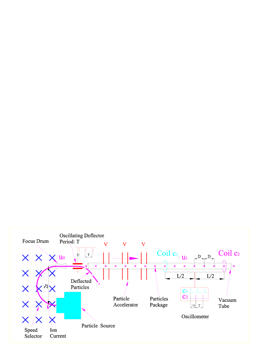
Figure 1: The flow chart and experimental scheme to test the mass-energy relation

1. The particles with unit charge are produced by the particles source, and the ones at initial speed $v_{0}$ are selected by a homogeneous magnetic field. By adjusting the radius $r$, we can control the initial speed $v_{0}$ of the particles.

2. The particle beam with speed $v_{0}$ is focused by a focus drum.

3. The focused particle beam is controlled by an oscillating deflector with signal period $T$. When the plate condenser is charged with voltage $\bar{U}$, the particles are deflected and can not enter the vacuum tube. Only in the moment the voltage $\bar{U}$ is removed, a package of charged particle moves into the vacuum tube to be accelerated and tested. Then we get a series of particle packages with periodic intervals

   $$v_{0}T\to D=v_{1}T.$$ (5)

4. The series-wound accelerator is constructed by a set of uniform electrodes, which can be charged with high voltage $V$. When the selected particles pass though one pair electrodes, each particle receives an energy increment $\delta E=eV$, which converts into its kinetic energy. If $n$ pair electrodes are charged, then we get the total kinetic energy increment for each particle

   $$K=E(v_{1})-E(v_{0})=n\delta E=neV.$$ (6)

   (3) and (6) establish the connection between the speed $v$ and $nV$.

5. An oscillometer with high frequency(e.g. 100MHz) is placed at the midpoint between the two solenoid coils. When one particles package pass trough one coil, an electromotive signal is generated in the coil and the signal can by detected by the oscillometer. The time increment between the package passing trough two solenoid coils $c_{0}$ and $c_{1}$ is

   $$\Delta t=\frac{L}{v_{1}},$$ (7)

   which can be measured by the oscillometer.

6. Adjusting the deflecting period $T=\Delta t$ until we get two series of periodic pulses which can be completely overlapped, then by (5) and (7) the final speed $v_{1}$ of the particles can be exactly calculated as

   $$v_{1}=\frac{L}{T}.$$ (8)

   If the distance between two coils $c_{0}$ and $c_{1}$ is set as $L=6m$, then the deflecting frequency $\nu\sim 50$MHz or $T\sim 0.02\mu\rm s$.

7. Since the distance $L$ and the period $T$ can be adjusted to very high accuracy, so we can calculate the true energy-speed relation $E=m(v)c^{2}$ according to the measured results.

In what follows, we take (3) as example to show the dada treatment, i.e. we determine the constants $(M_{0},M_{1},M_{F})$ by fitting the curve $f(v_{1},V)=0$ defined by (3). Now we make some simplification of (6). At first, we can solve the static mass $M_{0}$ at low energy $v=\widetilde{v}_{1}\ll c$ as follows. Assume the voltage $V=V_{0}$, in this nonrelativistic case, we have the approximation of (6) as follows

$$neV_{0} \dot{=} \frac{1}{2}(M_{0}-2M_{1}+M_{F})(\widetilde{v}_{1}^{2}-v_{0}^{2}).$$ (9)

Then we get

$$\left\{\begin{array}[]{lll}M_{0}&=&m_{s}+2M_{1}-M_{F},\\ E_{0}&=&m_{s}+2M_{1}-M_{F}+\frac{1}{2}m_{s}u_{0}^{2}\dot{=}E(v_{0}),\\ m_{s}&\equiv&2neV_{0}(\widetilde{v}_{1}^{2}-v_{0}^{2})^{-1},\end{array}\right.$$ (13)

where $m_{s}$ is the nonrelativistic static mass of the particle in classical sense. Therefore, we only need to determine two little coefficients $(M_{1},M_{F})$ at high energy.

By (3), (6) and (13), we have the following relation

$$(2-v_{1}^{2})M_{1} - \left(1+\ln\sqrt{1-v_{1}^{2}}\right)M_{F}\left\{=E(v_{1})\sqrt{1-v_{1}^{2}}-m_{s}\right.\qquad{\rm(by\leavevmode\nobreak\ (\ref{1.3})\leavevmode\nobreak\ and\leavevmode\nobreak\ (\ref{1.6}))}$$ (14)

$$= \left.[neV+E(v_{0})]\sqrt{1-v_{1}^{2}}-m_{s}\right\}\qquad\qquad\qquad\qquad\quad\leavevmode\nobreak\ {\rm(by\leavevmode\nobreak\ (\ref{1.4})\leavevmode\nobreak\ and\leavevmode\nobreak\ (\ref{1.6}))}$$

$$\dot{=} (neV+\frac{1}{2}m_{s}v_{0}^{2})\sqrt{1-v_{1}^{2}}-\frac{m_{s}v_{1}^{2}}{1+\sqrt{1-v_{1}^{2}}}+(2M_{1}-M_{F})\sqrt{1-v_{1}^{2}}.$$

Denoting

$$w=\frac{v_{1}^{2}}{1+\sqrt{1-v_{1}^{2}}},\qquad U=(neV+\frac{1}{2}m_{s}v_{0}^{2})c^{-2},$$ (15)

and substituting it into (14), we get

$$w^{2}M_{1}-\left[w+\ln({1-w})\right]M_{F}=({1-w})U-wm_{s}.$$ (16)

(16) is a linear equation of $(M_{1},M_{F})$, which can be easily solved by the method of least squares from a sequence of measured data $(U_{i},w_{i}),i=1,2,\cdots,N$. Define the $N$-dimensional vectors $(\vec{a},\vec{b},\vec{f})$ by,

$$\vec{a} = (w_{1}^{2},w_{2}^{2},\cdots,w_{N}^{2}),$$ (17)

$$\vec{b} = -\left[w_{1}+\ln({1-w_{1}}),w_{2}+\ln({1-w_{2}}),\cdots,w_{N}+\ln({1-w_{N}})\right],$$ (18)

$$\vec{f} = [({1-w_{1}})U_{1}-w_{1}m_{s},({1-w_{2}})U_{2}-w_{2}m_{s},\cdots,({1-w_{N}})U_{N}-w_{N}m_{s}].$$ (19)

Then the solution of the least square is given by

$$M_{1}=\frac{1}{D}[\vec{b}\leavevmode\nobreak\ ^{2}\vec{a}-(\vec{a}\cdot\vec{b})\vec{b}]\cdot\vec{f},\quad M_{F}=\frac{1}{D}[\vec{a}^{2}\vec{b}-(\vec{a}\cdot\vec{b})\vec{a}]\cdot\vec{f},\quad D=\vec{b}\leavevmode\nobreak\ ^{2}\vec{a}^{2}-(\vec{a}\cdot\vec{b})^{2},$$ (20)

For an electron, we have the typical order of magnitude for the parameters in (16),

$$w\sim 1,\qquad U\sim m_{s}\sim 1{\rm MeV}.$$ (21)

So a meaningful test depends on the precision of the measurement data $(w_{i},U_{i})$, which should be of relative errors less than $10^{-4}$. How to promote the precision of the measurement is the key for the success of a test.

Some possible solutions and its implications:

1. If $M_{F}=0$ and $M_{1}=0$, which means the Einstein’s mass-energy strictly holds, and the particles can not be described by the classical fields, because a linear spinor is unstable for a standing wave.

2. If $M_{F}=0$ and $M_{1}\neq 0$, this kind of particles has not nonlinear self-potential, and the balance of the particles should be explained by scalar and vectorial interactive fields.

3. If $M_{F}\neq 0$, which means particle including nonlinear potential, which leads to some unusual effectsgu1 ; gu2 ; spn1 .

so no matter what result the experiment provides, the implication is always important and fundamental.

From the above analysis, we find the test of the energy-speed relation can provide new insights into the structure of the fundamental particles and space-time. An exact measurement of the energy-speed relation is a shortcut to disclose the secrets of the fundamental particles and interactive potentials, as well as the nature of dark matter and dark energy. So this experiment is of fundamental significance, which may clarify a number of puzzles in physics.

References

- (1) Einstein, A. Ann. der Phys. 18, 639-641 (1905).
- (2) S. Rainville, et al., A Direct Test of , Nature, 438, 22, 2005, p.1096.
- (3) Ezzat G. Bakhoum, Why Emerges in the Process of Neutron Capture, arXiv:0705.3191
- (4) Y. Q. Gu, New Approach to N-body Relativistic Quantum Mechanics, Int. J. Mod. Phys. A22:2007-2020(2007), arXiv:hep-th/0610153
- (5) Y. Q. Gu, A Cosmological Model with Dark Spinor Source, Int. J. Mod. Phys. A22:4667-4678(2007), arXiv:gr-qc/0610147
- (6) V. Adanhounme, A. Adomou, F. P. Codo, M. N. Hounkonnou, Nonlinear spinor field equations in gravitational theory: spherical symmetric soliton-like solutions, arXiv:1211.3388
- (7) M. O. Ribas, et al., Phys. Rev. D 72, (2005)123502, arXiv:gr-qc/0511099.
- (8) H. J. de Vega, Dark energy from cosmological neutrino condensation, arXiv:astro-ph/0701212
- (9) S. I. Vacaru Spinor and Twistor Geometry in Einstein Gravity and Finsler Modifications, Adv. Appl. Clifford Algebras 25 (2015) 453-483,
- (10) Y. Q. Gu, Local Lorentz Transformation and Mass-Energy Relation of Spinor, arXiv:hep-th/0701030v3