Quantization of Skyrmions

Abstract

The Skyrme model is a nonlinear classical field theory which models the strong interaction between atomic nuclei. In order to compare the predictions of the Skyrme model with nuclear physics, it has to be quantized. We show, summarizing earlier work, how the rational map ansatz can be employed to calculate the Finkelstein-Rubinstein constraints which arise during quantization. Then we give an overview of current results on the quantum ground states in the Skyrme model. We end with an outlook on future work.

1 Introduction

The Skyrme model is a classical field theory modelling the strong interaction between atomic nuclei [1]. It has to be quantized in order to compare it to nuclear physics. In [2, 3], Adkins et al. quantized the translational and rotational zero-modes of the $B=1$ Skyrmion for zero and nonzero pion mass, respectively, and obtained good agreement with experiment. A subtle point is that Skyrmions can be quantized as fermions as has been shown in [4]. Solitons in scalar field theories can consistently be quantized as fermions provided that the fundamental group of configuration space has a ${\mathbb{Z}}_{2}$ subgroup generated by a loop in which two identical solitons are exchanged.

The quantization of Skyrmions has a long history. The $B=2$ Skyrmion with axial symmetry was quantized in [5, 6, 7] using the zero-mode quantization. Later, the approximation was improved by taking massive modes into account [8]. The $B=3$ Skyrmion was first quantized in [9] and the $B=4$ Skyrmion in [10]. Irwin performed a zero-mode quantization for $B=4-9$ [11] using the monopole moduli space as an approximation for the Skyrmion moduli space. The physical predictions of the Skyrme model for various baryon numbers were also discussed in [12]. Our aim here is to summarize the approach in [13, 14] and give an overview on current progress and trends. Section 2 gives a brief introduction to the Skyrme model and describes the rational map ansatz from a more topological point of view. Section 3 describes the approach of Finkelstein and Rubinstein to the quantization of Skyrmions, [4], and shows how the rational map ansatz can be used to calculate the Finkelstein-Rubinstein constraints. In Section 4, we describe the calculation of the quantum ground states in the Skyrme model using the zero-mode approximation. We end with a discussion of which other physical effects have to be taken into account.

2 The Skyrme Model

The Skyrme model is a classical field theory of pions. The basic field is the $SU(2)$ valued field $U({\bf x},t)$ where ${\bf x}\in{\mathbb{R}}^{3}$. The static solutions can be obtained by varying the following energy

$$E=\int\left(-\frac{1}{2}{\rm Tr}(R_{i}R_{i})-\frac{1}{16}{\rm Tr}([R_{i},R_{j}][R_{i},R_{j}])-m^{2}{\rm Tr}(U-1)\right)d^{3}x,$$ (1)

where $R_{i}=(\partial_{i}U)U^{\dagger}$ is a right invariant $su(2)$ valued current, and $m$ is a parameter proportional to the pion mass $m_{\pi}$, [15]. See also [16] for a discussion of alternative pion mass terms. In (1) we employed the “geometric units” in which length is measured in units of $2/ef_{\pi}$ and energy in units of $f_{\pi}/4e$. The parameters $f_{\pi}$ and $e$ are known as the pion decay constant and the Skyrme constant, respectively. In order to have finite energy, Skyrme fields have to take a constant value, $U(|{\bf x}|=\infty)=1$, at infinity. Due to this boundary condition, all the points $|{\bf x}|=\infty$ can be identified and named “$\infty$”. By a one-point compactification, the domain ${\mathbb{R}}^{3}$ together with “$\infty$” is topologically the three dimensional sphere $S^{3}$. Recall that the group $SU(2)$ as a manifold is also a three-sphere. Therefore, from a topological point of view the Skyrme field $U$ can be regarded as a map $U:S^{3}\to S^{3}$, and such maps are characterized by an integer-valued winding number. This topological charge is interpreted as the baryon number, which for our purposes can be thought of as the number of protons and neutrons. It is given by the following integral

$$B=-\frac{1}{24\pi^{2}}\int\epsilon_{ijk}{\rm Tr}(R_{i}R_{j}R_{k})d^{3}x.$$ (2)

We will denote the configuration space of Skyrmions by $Q$. $Q$ splits into connected components $Q_{B}$ labelled by the topological charge. Furthermore, the energy of configurations in $Q_{B}$ is bounded below by $E\geq 12\pi^{2}B,$ [17].

2.1 Rational Maps

In this section, we describe the rational map ansatz [18] which is a very successful approximation to minimal energy Skyrme configurations. The most convenient way for obtaining the explicit formula is the geometric approach of Manton [19, 20]. In the following, we describe the construction in a more mathematical way, which will allow us to apply theorems from algebraic topology. The key idea is to view the rational map ansatz as a suspension.

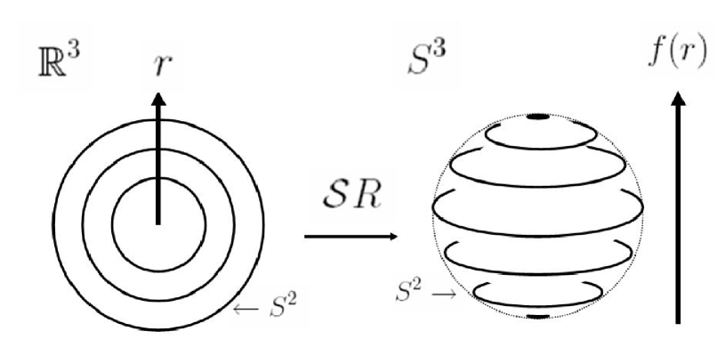
Figure 1: An illustration of the suspension map for the rational map ansatz. Concentric spheres around the origin in ${\mathbb{R}}^{3}$ are mapped to spheres of latitude in $S^{3}$. Due to the boundary conditions, the sphere at $r=\infty$ can be regarded as one point.

Given an interval $I=[0,1]$ and a manifold $M$, we can define the suspension ${\cal S}M$ by taking the Cartesian product $I\times M$ and then collapsing $\{0\}\times M$ to a point and also collapsing $\{1\}\times M$ to a point. A very important example is the suspension of spheres, namely, ${\cal S}S^{n}=S^{n+1}$. The standard polar coordinates are a smoothed-out version of a suspension. However, not only spaces, but also maps can be suspended. Consider the map

$$R:S^{2}\to S^{2},z\mapsto R(z),$$ (3)

which is a map between Riemann spheres. $z$ and $R$ are the standard complex coordinates obtained by stereographic projection. Now, both spheres can be suspended and we obtain $U={\cal S}R$.

$$U:S^{3}\to S^{3},(r,z)\mapsto(f(r),R(z)).$$ (4)

The boundary conditions are $f(0)=\pi$ and $f(\infty)=0$, so the end points of the “interval” $[0,\infty)$ are mapped to the endpoints of the interval $[0,\pi]$. For a graphical illustration of this construction, see figure 1.

There is one further condition which makes the rational map ansatz particularly easy to use, namely, to consider only rational maps $R(z)$. Rational maps are holomorphic maps between Riemann spheres, and they can be written as ratios of two polynomials $p(z)$ and $q(z)$ which have no common factors, $R(z)=p(z)/q(z)$. The maximal polynomial degree of these polynomials $p(z)$ and $q(z)$ is also the topological degree of the rational map $R(z)$. Suspensions have good properties with respect to homotopy groups. Of particular importance is the Freudenthal suspension theorem [21, Corollary 4.24]. One consequence of this theorem is that rational maps $R(z)$ of degree $B$ give rise to Skyrme fields $U$ also of degree $B$. When the ansatz (4) is inserted into equation (1) we obtain

$$E=4\pi\int\left(r^{2}{f^{\prime}}^{2}+2B({f^{\prime}}^{2}+1)\sin^{2}f+{\cal I}\frac{\sin^{4}f}{r^{2}}+2m^{2}r^{2}(1-\cos f)\right){\rm d}r,$$ (5)

where

$${\cal I}=\frac{1}{4\pi}\int\left(\frac{1+|z|^{2}}{1+|R|^{2}}\left|\frac{{\rm d}R}{{\rm d}z}\right|\right)^{4}\frac{2i~{}{\rm d}z{\rm d}{\bar{z}}}{(1+|z|^{2})^{2}},$$ (6)

and $B$ can be written as

$$B=\frac{1}{4\pi}\int\left|\frac{{\rm d}R}{{\rm d}z}\right|^{2}\frac{2i~{}{\rm d}z{\rm d}{\bar{z}}}{(1+|R|^{2})^{2}}.$$ (7)

Note that $B$ is the topological charge, and therefore an integer, whereas ${\cal I}$ is a positive real number which depends on the given rational map. From a geometric point of view, ${\cal I}$ measures the angular strain orthogonal to the radial direction. It also has an interesting interpretation as a possible Morse function on the moduli space of monopoles [18]. Now, we can first calculate the rational map which minimizes the integral ${\cal I}$ and then solve the Euler-Lagrange equation for $f(r)$ subject to the boundary conditions $f(0)=\pi$ and $f(\infty)=0$. The rational maps which minimize ${\cal I}$ for $m=0$ have been determined numerically in [22, 23] for all $B\leq 40$.

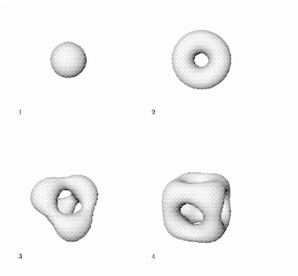
Figure 2: Level sets of constant energy density for Skyrmions of baryon number $B=1,\dots 4.$ (Figure taken from [24].)

In figure 2, we show the lowest four “Skyrmions”, that is the minimal energy configurations for baryon numbers $B=1,\dots,4$. Here, we plot the level sets of constant energy density, namely the surfaces in ${\mathbb{R}}^{3}$ where the integrand of $(\ref{energy})$ has a given value. It is apparent that the configurations in figure 2 are very “symmetric”. The surface of constant energy density for $B=1$ is a sphere which has spherical symmetry, whereas $B=2$ has axial symmetry, and $B=3$ and $4$ have tetrahedral and cubic symmetry, respectively. In fact, not only the energy density is symmetric but also the Skyrme fields. By symmetry we mean that a rotation in space followed by a rotation in target space leaves the Skyrmion invariant. Namely,

$$U({\bf x})=AU\left(D(A^{\prime}){\bf x}\right)A^{\dagger},$$ (8)

where $A$ and $A^{\prime}$ are $SU(2)$ matrices and $D(A^{\prime})$ is the associated $SO(3)$ rotation. These symmetries will play a very important role for the calculation of quantum ground states in the Skyrme model.

Another curious fact about the pictures in figure 2 are the “holes”, that is areas of particularly low energy density. The $B=4$ Skyrmion has six holes forming the faces of a cube, and the $B=3$ Skyrmion has $4$ holes. There is an easy way of understanding these “holes” from the rational map ansatz [18]. The angular dependence of the energy density in (5) strongly depends on

$$\frac{{\rm d}R}{{\rm d}z}=\frac{p^{\prime}(z)q(z)-q^{\prime}(z)p(z)}{q(z)^{2}},$$ (9)

as can be seen from equations (6) and (7). The numerator of equation (9) is known as the Wronskian and is generally a polynomial of degree $2B-2$. So, the zeros of the Wronskian give the faces of the Skyrme configurations. Similar polynomials also exist whose zeros correspond to the edges and vertices of Skyrme configurations.

Note that the restriction that $R(z)$ is a holomorphic map can be lifted and a generalized rational map ansatz can be introduced [25]. This generalized ansatz has been shown to improve the approximation for the energy significantly for the Skyrmions of degree $B=2,3,$ and $4$ in figure 2, and it also captures the singularity structure of Skyrmions better. However, it is difficult to use for higher baryon number, and from the point of view of discussing symmetries the original rational map ansatz is sufficient and easier to use.

3 Quantization of Skyrmions

In the following, we recall the ideas of Finkelstein and Rubinstein [4] on how to quantize a scalar field theory and obtain fermions. We then show how to use the rational map ansatz to calculate the Finkelstein-Rubinstein constraints.

3.1 Finkelstein-Rubinstein Constraints

In quantum field theory, there are two types of particles, namely bosons and fermions. If two identical particles are exchanged then nothing happens if these particles are bosons, whereas the wave function of the fermions changes by a factor of $(-1)$. When a boson wave function is rotated by $2\pi$, it remains invariant. However, if a fermion wave function is rotated by $2\pi$, then it changes by a factor of $(-1)$. The latter statement is a consequence of the spin-statistic theorem. In quantum field theory bosons are usually described by scalar, vector or tensor fields whereas fermions are represented by spinors.

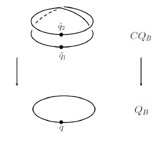
Figure 3: This figure illustrates, schematically, the covering map. Both points ${\tilde{q}}_{1}$ and ${\tilde{q}}_{2}\in CQ_{B}$ correspond to the same point $q\in Q_{B}$. Given a loop in configuration space starting at $q$ we can lift this loop to give a path in $CQ_{B}$ which will end at ${\tilde{q}}_{2}$, if the original loop is non-contractible, and will end at ${\tilde{q}}_{1}$ otherwise.

So, how do we quantize the Skyrme model, which is a scalar field theory, such that Skyrmions can model atomic nuclei, which consist of fermions? The key idea by Finkelstein and Rubinstein is to consider wave functions on the covering space of configuration space. Note that $Q_{B}$, the configuration space of Skyrme configurations of degree $B$, has fundamental group $\pi_{1}(Q_{B})\cong{\mathbb{Z}}_{2}$, in other words, its covering space $CQ_{B}$ is a double cover.

Recall that one can think of the covering space $CQ_{B}$ as the space of equivalence classes of paths in the space $Q_{B}$. Figure 3 illustrates this construction. Consider the two points ${\tilde{q}}_{1}$ and ${\tilde{q}}_{2}\in CQ_{B}$ which correspond to the point $q\in Q_{B}$. These two points are joined by a path in $CQ_{B}$ which projects to a non-contractible loop in $Q_{B}$. This gives us a way of examining continuous symmetries of Skyrme configurations. A continuous symmetry of a configuration $q$ can be thought of as an induced loop in configuration space. The symmetry also acts on covering space, namely, if we apply the symmetry to ${\tilde{q}}_{1}$ we obtain ${\tilde{q}}_{1}$ if the induced loop is contractible, and ${\tilde{q}}_{2}$ if it is not contractible.

We can now formally define a wave function $\psi$ as

$$\psi:CQ_{B}\to{\mathbb{C}},{\tilde{q}}\mapsto\psi({\tilde{q}}),$$ (10)

and impose the Finkelstein-Rubinstein constraint that $\psi({\tilde{q}}_{1})=-\psi({\tilde{q}}_{2})$ where ${\tilde{q}}_{1}$ and ${\tilde{q}}_{2}$ are defined as above. In the following, we are particularly interested in loops which arise from the symmetries (8). Using the Finkelstein-Rubinstein constraint, we see that a rotation by $\alpha$ around axis ${\bf n}$ in space followed by a rotation by $\beta$ in target space around axis ${\bf N}$ gives

$$\exp\left(-i\alpha{\bf n}\cdot{\hat{\bf J}}\right)\exp\left(-i\beta{\bf N}\cdot{\hat{\bf I}}\right)\psi({\tilde{q}})=\chi_{FR}~{}\psi({\tilde{q}}),$$ (11)

where

$$\chi_{FR}=\left\{\begin{array}[]{cc}1&{\rm if~{}the~{}induced~{}loop~{}is~{}contractible,}\\ -1&{\rm otherwise.}\end{array}\right.$$ (12)

Here ${\hat{\bf J}}$ and ${\hat{\bf I}}$ are spin operators in space and target space, respectively. For notational convenience, we will refer to a rotation in target space as an isorotation. Before we discuss how to calculate the Finkelstein-Rubinstein phase $\chi_{FR}$ using the rational map ansatz, we summarize some important and well-known results. Giulini showed that a $2\pi$ rotation of a Skyrmion gives rise to $\chi_{FR}=(-1)$ if and only if the baryon number $B$ is odd, [27]. Finkelstein and Rubinstein showed in [4] that a $2\pi$ rotation of a Skyrmion of degree $B$ is homotopic to an exchange of two Skyrmions of degree $B$. This also implies that an exchange of two identical Skyrmions gives rise to $\chi_{FR}=(-1)$ if and only if their baryon number $B$ is odd. In [13] it was shown that a $2\pi$ isorotation of a Skyrmion also gives rise to $\chi_{FR}=(-1)$ if and only if the baryon number $B$ is odd. These results agree with the physical intuition since atomic nuclei can be modelled by interacting point-like fermionic particles.

3.2 Rational Maps and Finkelstein-Rubinstein constraints

In this section, we show how to calculate the Finkelstein-Rubinstein phase $\chi_{FR}\in\pi_{1}(Q_{B})$ from the rational map ansatz [13, 14]. Using the Freudenthal suspension theorem [21, Corollary 4.24], the following theorem has been proved in [13].

Theorem 3.1 (S.K.)

The rational map ansatz induces a surjective homomorphism
$\pi_{1}(Rat_{B}^{*})\to\pi_{1}(Q_{B}^{*}).$

Here $Rat_{B}^{*}$ denotes the space of based rational maps of degree $B$. Based rational maps satisfy the base point condition $R(\infty)=1$. The notation $Q_{B}^{*}$ just emphasizes that Skyrme configurations are also based because $U(\infty)=1$. The theorem gives us a way to calculate $\chi_{FR}$ provided we know the fundamental group of rational maps. The following theorem gives us the necessary information.

Theorem 3.2 (Segal)

$\pi_{1}(Rat_{B}^{*})\cong{\mathbb{Z}}$ and it is generated by moving a zero once around a pole.

Note that a map $R\in Rat_{B}^{*}$ can be written as

$$R(z)=\frac{z^{B}+a_{B-1}z^{B-1}+\dots+a_{0}}{z^{B}+b_{B-1}z^{B-1}+\dots+b_{0}}=\prod\limits_{i,j=1}^{B}\frac{z-z_{i}}{z-p_{j}}.$$ (13)

So, a based rational map $R(z)$ can be parameterized solely in terms of its zeros $z_{i}$ and poles $p_{j}$. Given a loop $L$ that moves zeros $z_{i}$ and poles $p_{j}$ around in the complex plane as a function of $\phi\in[0,\Phi]$, let

$$N(L)=\frac{i}{2\pi}\sum\limits_{i,j=1}^{B}\int\limits_{0}^{\Phi}\frac{\left(z_{i}^{\prime}(\phi)-p_{j}^{\prime}(\phi)\right){\rm d}\phi}{\left(z_{i}(\phi)-p_{j}(\phi)\right)}.$$ (14)

With this definition and using Cauchy’s theorem it is straight forward to prove the following lemma.

Lemma 3.3

$N(L)$ is a homotopy invariant and counts the number of times zeros move around poles. Therefore, $N(L)$ provides an isomorphism $\pi_{1}(Rat_{B}^{*})\to{\mathbb{Z}}.$

The above lemma gives us a way to calculate $N(L)$ for any loop in the space of based rational maps numerically. However, the fact that $N(L)$ is a homotopy invariant allows us to make even more progress. Let us consider the axially symmetric map

$$R(z)=\frac{z^{B}-b}{z^{B}+b}.$$ (15)

We can now consider a loop as in (11), generated by a rotation by an angle $\alpha$ around the $z$-axis followed by a rotation by an angle $\beta$ around the $X$-axis in target space. This choice of axes guarantees that the whole loop respects the boundary condition $R(\infty)=1$. For the rational map (15) it is easy to see how the zeros and poles behave as the rotation angle goes from $0$ to $\alpha$ and $\beta$, respectively. Using formula (14) we can evaluate $N(L)$ for this loop explicitly and obtain

$$N=\frac{B}{2\pi}\left(B\alpha-\beta\right).$$ (16)

Surprisingly, (16) can be used in a much more general context.

Theorem 3.4 (S.K.)

The value of $N$ for a given symmetry of a rational map $R\in Rat_{B}$ only depends on the rotation angle $\alpha$ and the isorotation angle $\beta$, where the angles are defined such that $R(z_{-{\bf n}})=R_{\bf N}$. It is given by (16).

There is a choice for the sign of $\alpha$ which corresponds to the choice of the rotation axis in space. Once the axis in space is fixed the rational map determines the sign of the rotation axis in target space via $R(z_{-{\bf n}})=R_{\bf N}$. Here $z_{-{\bf n}}$ is the complex coordinate of the point $-{\bf n}$ and similarly for $R_{{\bf N}}$. This condition is important since if the wrong sign for $\beta$ is used in (16) the value of $N$ might no longer be integer. Now, we can express the Finkelstein-Rubinstein phase $\chi_{FR}$ in terms of $N$ via the surjection

$$\chi_{FR}=(-1)^{N}.$$ (17)

It is important to emphasize that theorem 3.4 can only be used for Skyrme configurations which can be deformed into Skyrme fields obtained from the rational map ansatz while keeping the relevant symmetry [14]. This is clearly the case for $2\pi$ rotations. Hence, a $2\pi$ rotation of a Skyrmion of degree $B$ gives

$$\chi_{FR}=(-1)^{B^{2}},$$ (18)

which is equal to $(-1)$ if and only if $B$ is odd. Similarly, a $2\pi$ rotation in target space — a $2\pi$ isorotation — gives rise to

$$\chi_{FR}=(-1)^{B},$$ (19)

thus reproducing some of the results discussed at the end of the previous subsection.

Often a Skyrme configuration $U$ can be approximated by assuming that it consists of $K$ disjoint parts, each of which can be approximated as a Skyrmion of degree $B_{i}$ centered around $X_{i}$. Then the truncated rational map ansatz can be written as

$$U({\bf x})=\left\{\begin{array}[]{lc}U_{1}({\bf x}),&{\rm for~{}}|{\bf x}-{\bf X}_{1}|<L_{1},\\ \vdots&\vdots\\ U_{K}({\bf x}),&{\rm for~{}}|{\bf x}-{\bf X}_{K}|<L_{K},\\ 1,&{\rm otherwise,}\end{array}\right.$$ (20)

where the parameters $L_{i}$ are related to the size of the Skyrme configurations and the individual parts $U_{i}$ are well approximated by the rational map ansatz, subject to the boundary condition that $U_{i}({\bf x})=1$ for $|{\bf x}-{\bf X}_{i}|=L_{i}$. It is clear from formula (2) that the baryon number of this configuration is given by $B=B_{1}+\dots+B_{K}$. We can now use this ansatz to calculate the Finkelstein-Rubinstein constraints for Skyrme configuration which are symmetric under a $C_{n}^{k}$ symmetry. By $C_{n}^{k}$ symmetry we mean a rotation by $\alpha=\frac{2\pi}{n}$ followed by a rotation by $\beta=\frac{2\pi k}{n}$ in target space. This $C_{n}^{k}$ symmetry relates different Skyrmions $U_{B_{i}}$ with each other. For each individual Skyrmion, there are two possibilities. Either the centre of the Skyrmion lies on the symmetry axis, or the Skyrmion is part of an $n$-gon of Skyrmions which transform into each other. Assume that there are $l$ regular $n$-gons of Skyrmions with degree $B_{i}$ for $i=1,\dots,l$ and $m$ Skyrmions of degree ${\tilde{B}}_{j}$ for $j=1,\dots,m$ which are located on the symmetry axis. Then the Finkelstein-Rubinstein constraints for this configuration are given by

$$\chi_{FR}=(-1)^{N},~{}~{}~{}{\rm where}~{}N=\sum\limits_{i=1}^{l}B_{i}(nB_{i}-k)+\sum\limits_{j=1}^{m}{\tilde{B}}_{j}({\tilde{B}}_{j}-k)/n.$$ (21)

This approach is very well suited for calculating the Finkelstein-Rubinstein constraints for (local) minima which are only know numerically. Once, the minimal energy configuration has been calculated, we have to determine its symmetry, and in particular $C_{n}^{k}$ for a set of generators of the symmetry group. We confirm the symmetry by starting with a symmetric configuration given, for example, by the truncated rational map ansatz as initial condition and then letting this configuration relax into the same final configuration. The crucial point is that the relaxation method provides a homotopy from the initial to the final configuration which is invariant under the symmetry. Therefore, it is mathematically sound to calculate the Finkelstein-Rubinstein constraints using formula (21).

4 Results and Outlook

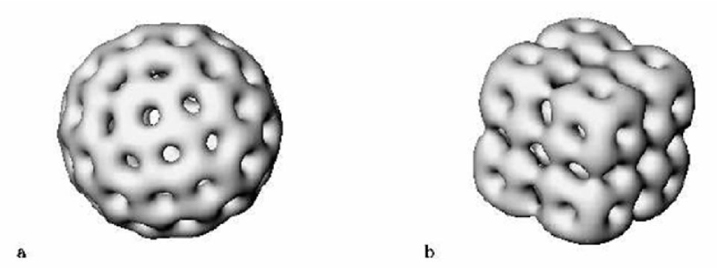
Figure 4: This figure shows energy level sets for two $B=32$ Skyrme configurations which have very low energy. For pion mass $m=0$ the rational map configuration (a) has lower energy whereas for higher values of $m$ the “cube” (b) has lower energy. (Figure taken from [28].)

In this section, we present the results of the approach described in the previous sections and also give a personal view on interesting current and future developments.

The simplest nontrivial application of this approach is to quantize the zero-modes around the classical minimal energy configurations in each sector $Q_{B}$, see [11, 13]. Then, the quantum ground state $|J\rangle|I\rangle$ is given by the lowest values of the angular momentum quantum numbers $J$ and $I$ which are compatible with the Finkelstein-Rubinstein constraints for the symmetries of the classical minimal energy configuration taken from [22]. For $B=1,\dots,4$ the results are promising. The Skyrme model reproduces the correct ground state for ${}^{1}_{1}$H ($|\frac{1}{2}\rangle|\frac{1}{2}\rangle$), the deuteron ${}^{2}_{1}$H ($|1\rangle|0\rangle$), ${}^{3}_{2}$He ($|\frac{1}{2}\rangle|\frac{1}{2}\rangle$), and the alpha-particle ${}^{4}_{2}$He ($|0\rangle|0\rangle$). The ground states corresponding to $B=8,12,16,20$ which are particularly stable are also correctly predicted as $|0\rangle|0\rangle$ states. In [14] states with even nucleon number $B$ have been examined further. The rational map ansatz gives restriction on what $C_{n}^{k}$ symmetry can be realized. These restrictions are compatible with the phenomenological even-even and odd-odd nucleons rule. However, for $B=5$ the predicted ground state does not agree with experiment. One might argue that this is not such a problem, since there is no stable nucleus with $5$ nuclei, however, this result marks the beginning of a trend. The predictions for odd nuclei are not reliable at all. In order to understand what is going wrong, we have to discuss the approximations in our approach in more detail. The zero-mode approximation neglects any deformations and vibrations of the Skyrme field and assumes that the Skyrmion rotates like a rigid body. Schematically, we obtain the following formula for the energy of a given state.

$$E\approx M_{{\rm classical}}+\frac{\hbar^{2}}{2\Theta_{J}}J(J+1)+\frac{\hbar^{2}}{2\Theta_{I}}I(I+1).$$ (22)

The above formula helps us to understand why the states with vanishing spin $J$ and vanishing isospin $I$ are modelled quite successfully by the classical minimals, namely, the contributions of the second and the third term vanish. For nucleon numbers $B$ which are divisible by two but not by four, the predictions only fail for $B=10,18,$ and $22$.

For fermions, however, the lowest possible quantum numbers are $J=\frac{1}{2}$, $I=\frac{1}{2}$, so that all three terms contribute in (22). These further contributions to the energy make it necessary to take local minima into account, when calculating quantum ground states. It is also important to allow the Skyrmions to deform while they are spinning, see [31] and references therein. A related approach constructing a quantum hamiltonian for spinning Skyrmions is described in [32]. Much work still needs to be done to understand spinning Skyrmions, both classically and quantum mechanically. In the former case, progress has been made by applying the theory of relative equilibria (work in progress).

However, there is another important effect, namely the effect of the pion mass term which is the last term in (1). In [15], it was shown that the physical value of the pion mass leads to shell-like configurations becoming unstable to squashing. While the minimals for small $B\leq 8$ hardly change, many new (local) minimal energy configurations have been found for larger $B$, see [28, 33, 34]. These new configurations are no longer shell-like, but often seem to be composed of $B=4$ cubes. The relation to the phenomenological alpha particle model is discussed in [33]. There is hope that the Skyrme model will one day be able to describe the low energy excited states for example for $B=12$ or $B=16$ as rotational bands related to different local minima in the same way as in the alpha particle model. In order to achieve this aim, we need a better understanding of the classical solutions, possibly including saddle point solutions in the Skyrme model [35]. This can be achieved by numerical simulations in connection with various analytic approximations, such as the instanton ansatz [36], including the version in hyperbolic space which takes account of the pion mass term [37], and generalizations of the rational map ansatz.

We also need to address the important problem of fixing the values of the Skyrme parameters $f_{\pi}$, $e$ and $m_{\pi}$. The original, and most widely used, set of Skyrme parameters has been proposed in [2, 3], by matching to the proton and the Delta mass. However, it has been shown that this matching condition can be considered to be an artifact of the rigid rotator approximation, [31]. The studies in [33] suggest that the effective pion mass $m$ should have the rather large value of $m\approx 1$. In [38], a 30% lower value of the Skyrme parameter was suggested in order to match a large range of nuclei masses to experimental data. A similar conclusion was reached in [39] by considering the electromagnetic properties of the quantized $B=6$ Skyrmion, describing ${}_{3}^{6}$Li.

Although there are many problems to overcome, there is cautious optimism that the Skyrme model can really teach us something about the behaviour of small to medium sized nuclei.

References

- [1] T. H. R. Skyrme, A Nonlinear field theory, Proc. Roy. Soc. Lond. A260: 127 (1961),
- [2] G. S. Adkins, C. R. Nappi and E. Witten, Static properties of nucleons in the Skyrme model, Nucl. Phys. B228: 552 (1983),
- [3] G. S. Adkins and C. R. Nappi, The Skyrme model with pion masses, Nucl. Phys. B233: 109 (1984),
- [4] D. Finkelstein and J. Rubinstein, Connection between spin, statistics, and kinks, J. Math. Phys. 9: 1762 (1968),
- [5] E. Braaten and L. Carson, The deuteron as a toroidal Skyrmion, Phys. Rev. D38: 3525 (1988),
- [6] V. B. Kopeliovich, Quantization of the rotations of axially symmetric systems in the Skyrme model, Sov. J. Nucl. Phys. 47: 949–953 (1988),
- [7] J. J. M. Verbaarschot, Axial symmetry of bound baryon number two solution of the Skyrme model, Phys. Lett. B195: 235 (1987),
- [8] R. A. Leese, N. S. Manton and B. J. Schroers, Attractive channel Skyrmions and the deuteron, Nucl. Phys. B442: 228 (1995), <hep-ph/9502405>,
- [9] L. Carson, B = 3 nuclei as quantized multiskyrmions, Phys. Rev. Lett. 66: 1406 (1991),
- [10] T. S. Walhout, Quantizing the four baryon skyrmion, Nucl. Phys. A547: 423 (1992),
- [11] P. Irwin, Zero mode quantization of multi-Skyrmions, Phys. Rev. D61: 114024 (2000), <hep-th/9804142>,
- [12] V. B. Kopeliovich, Characteristic predictions of topological soliton models, J. Exp. Theor. Phys. 93: 435–448 (2001), <hep-ph/0103336>,
- [13] S. Krusch, Homotopy of rational maps and the quantization of Skyrmions, Ann. Phys. 304: 103–127 (2003), <hep-th/0210310>,
- [14] S. Krusch, Finkelstein-Rubinstein constraints for the Skyrme model with pion masses, Proc. Roy. Soc. A462: 2001–2016 (2006), <hep-th/0509094>,
- [15] R. Battye and P. Sutcliffe, Skyrmions and the pion mass, Nucl. Phys. B705: 384–400 (2005), <hep-ph/0410157>,
- [16] V. B. Kopeliovich, B. Piette and W. J. Zakrzewski, Mass terms in the Skyrme model, Phys. Rev. D73: 014006 (2006), <hep-th/0503127>,
- [17] L. D. Faddeev, Some comments on the many dimensional solitons, Lett. Math. Phys. 1: 289 (1976),
- [18] C. J. Houghton, N. S. Manton and P. M. Sutcliffe, Rational maps, monopoles and Skyrmions, Nucl. Phys. B510: 507 (1998), <hep-th/9705151>,
- [19] N. S. Manton, Geometry of Skyrmions, Commun. Math. Phys. 111: 469 (1987),
- [20] S. Krusch, Skyrmions and the Rational Map Ansatz, Nonlinearity 13: 2163 (2000), <hep-th/0006147>,
- [21] A. Hatcher, Algebraic Topology, Cambridge University Press, Cambridge (2002).
- [22] R. A. Battye and P. M. Sutcliffe, Skyrmions, fullerenes and rational maps, Rev. Math. Phys. 14: 29 (2002), <hep-th/0103026>,
- [23] R. A. Battye, C. J. Houghton and P. M. Sutcliffe, Icosahedral Skyrmions, J. Math. Phys. 44: 3543–3554 (2003), <hep-th/0210147>,
- [24] R. A. Battye and P. M. Sutcliffe, Multi-soliton dynamics in the Skyrme model, Phys. Lett. B391: 150 (1997), <hep-th/9610113>,
- [25] C. J. Houghton and S. Krusch, Folding in the Skyrme model, J. Math. Phys. 42: 4079 (2001), <hep-th/0104222>,
- [26] S. Krusch and J. M. Speight, Fermionic quantization of Hopf solitons, Commun. Math. Phys. 264: 391–410 (2006), <hep-th/0503067>,
- [27] D. Giulini, On the possibility of spinorial quantization in the Skyrme model, Mod. Phys. Lett. A8: 1917 (1993), <hep-th/9301101>,
- [28] R. Battye and P. Sutcliffe, Skyrmions with massive pions, Phys. Rev. C73: 055205 (2006), <hep-th/0602220>,
- [29] D. Auckly and J. M. Speight, Fermionic quantization and configuration spaces for the Skyrme and Faddeev-Hopf models, Commun. Math. Phys. 263: 173–216 (2006), <hep-th/0411010>,
- [30] B. M. A. G. Piette and D. H. Tchrakian, Topologically stable soliton in the U(1) gauged Skyrme model, Phys. Rev. D62: 025020 (2000), <hep-th/9709189>,
- [31] R. A. Battye, S. Krusch and P. M. Sutcliffe, Spinning Skyrmions and the Skyrme parameters, Phys. Lett. B626: 120–126 (2005), <hep-th/0507279>,
- [32] C. Houghton and S. Magee, A zero-mode quantization of the Skyrmion, Phys. Lett. B632: 593–596 (2006), <hep-th/050909>,
- [33] R. Battye, N. S. Manton and P. Sutcliffe, Skyrmions and the alpha-particle model of nuclei (2006), <hep-th/0605284>,
- [34] C. Houghton and S. Magee, The effect of pion mass on Skyrme configurations (2006), <hep-th/0602227>,
- [35] S. Krusch and P. Sutcliffe, Sphalerons in the Skyrme model, J. Phys. A37: 9037 (2004), <hep-th/0407002>,
- [36] M. F. Atiyah and N. S. Manton, Skyrmions from instantons, Phys. Lett. B222: 438 (1989),
- [37] M. Atiyah and P. Sutcliffe, Skyrmions, instantons, mass and curvature, Phys. Lett. B605: 106–114 (2005), <hep-th/0411052>,
- [38] V. B. Kopeliovich, A. M. Shunderuk and G. K. Matushko, Mass splittings of nuclear isotopes in chiral soliton approach, Phys. Atom. Nucl. 69: 120–132 (2006), <nucl-th/0404020>,
- [39] N. S. Manton and S. W. Wood, Reparametrising the Skyrme Model using the Lithium-6 Nucleus (2006), <hep-th/0609185>.