QED(1+1) on the Light Front and its implications
for semiphenomenological methods in QCD(3+1)

Abstract

A possibility of semiphenomenological description of vacuum effects in QCD quantized on the Light Front (LF) is discussed. A modification of the canonical LF Hamiltonian for QCD is proposed, basing on the detailed study of the exact description of vacuum condensate in QED(1+1) that uses correct form of LF Hamiltonian.

1. Introduction

First of all let us remind briefly basic advantages and main difficulties of the quantization on the LF (by the ”LF” we mean the hyperplane $x^{+}=0$ in Dirac [1] ”light cone” coordinates $x^{\pm}=(x^{0}\pm x^{1})/\sqrt{2}$, with the $x^{+}$ playing the role of time).

1. LF momentum operator $P_{-}=(P_{0}-P_{1})/\sqrt{2}\geq 0$ is nonnegative for states with $p_{0}\geq 0$, $p^{2}\geq 0$. Like usual space momentum it is kinematical (quadratic in fields) generator of translations (in LF coordinate $x^{-}$). The vacuum state can be identified with the eigenstate of the $P_{-}$ with minimal eigenvalue $p_{-}=0$.

The field operator $\Phi(x)$ at $x^{+}=0$ can be classified in $p_{-}$ via the following form of Fourier decomposition (here the $\Phi(x)$ is taken to be a scalar field):

$$\halign{\hbox to\displaywidth{$\hfil\displaystyle#\hfil$}\cr 0.0pt{\hfil$\displaystyle\hskip 10.00002pt minus 10.00002pt\Phi(x)=\int\limits_{0}^{\infty}\frac{dp_{-}}{\sqrt{2p_{-}}}\left(a(p_{-},x^{\bot})e^{-ip_{-}x^{-}}+{\rm h.c.}\right),\hfil\hskip 10.00002pt minus 10.00002pt(1)\hfilneg\crcr}}$$

where $a(p_{-},x^{\bot})$ and $ia^{+}(p_{-},x^{\bot})$ at $p_{-}>0$ enter into scalar field action as canonically conjugated variables on the LF:

$$\halign{\hbox to\displaywidth{$\hfil\displaystyle#\hfil$}\cr 0.0pt{\hfil$\displaystyle\hskip 10.00002pt minus 10.00002pt[a(p_{-},x^{\bot}),a({p^{\prime}}_{-},{x^{\prime}}^{\bot})]=0,\hfil\hskip 10.00002pt minus 10.00002pt(2)\hfilneg\crcr}}$$

$$\halign{\hbox to\displaywidth{$\hfil\displaystyle#\hfil$}\cr 0.0pt{\hfil$\displaystyle\hskip 10.00002pt minus 10.00002pt[a(p_{-},x^{\bot}),a^{+}({p^{\prime}}_{-},{x^{\prime}}^{\bot})]=\delta(p_{-}-{p^{\prime}}_{-})\delta(x^{\bot}-{x^{\prime}}^{\bot}).\hfil\hskip 10.00002pt minus 10.00002pt(3)\hfilneg\crcr}}$$

The LF momentum operator is

$$\halign{\hbox to\displaywidth{$\hfil\displaystyle#\hfil$}\cr 0.0pt{\hfil$\displaystyle\hskip 10.00002pt minus 10.00002ptP_{-}=\int dx^{-}\int d^{2}x^{\bot}(\partial_{-}\Phi)^{2}=\int d^{2}x^{\bot}\int\limits_{0}^{\infty}dp_{-}p_{-}a^{+}(p_{-},x^{\bot})a(p_{-},x^{\bot})\geq 0.\hfil\hskip 10.00002pt minus 10.00002pt(4)\hfilneg\crcr}}$$

”Physical vacuum” $|0\rangle$ is defined like ”mathematical” one:

$$\halign{\hbox to\displaywidth{$\hfil\displaystyle#\hfil$}\cr 0.0pt{\hfil$\displaystyle\hskip 10.00002pt minus 10.00002pta(p_{-},x^{\bot})|0\rangle=0,\quad p_{-}>0.\hfil\hskip 10.00002pt minus 10.00002pt(5)\hfilneg\crcr}}$$

This simplicity of the description of the vacuum is main advantage of the quantization on the LF.

2. The problem of searching the spectrum of bound states can be considered nonperturbatively in LF Fock space basis $\{a^{+}....a^{+}|0\rangle\}$ by solving the following equations:

$$\halign{\hbox to\displaywidth{$\hfil\displaystyle#\hfil$}\cr 0.0pt{\hfil$\displaystyle\hskip 10.00002pt minus 10.00002ptP_{+}|\Psi\rangle=p_{+}|\Psi\rangle,\quad P_{-}|\Psi\rangle=p_{-}|\Psi\rangle,\quad P_{\bot}|\Psi\rangle=0.\hfil\hskip 10.00002pt minus 10.00002pt(6)\hfilneg\crcr}}$$

Then $m^{2}=p^{2}=2p_{+}p_{-}$. This can be used in attempts to approach nonperturbatively to bound state problem in Quantum Chromodynamics (QCD).

3. Main difficulties of LF quantization are related with singularities at $p_{-}\to 0$.

Possible regularizations are

(a) cutoff in $p_{-}\;\;(p_{-}\geq\varepsilon>0)$, or

(b) the ”DLCQ” regularization (”DLCQ” means Discretized Line Cone Quantization), i.e. the cutoff in $x^{-}$ ($|x^{-}|\leq L$ plus periodic boundary conditions, and $p_{-}=\frac{\pi n}{L}$, $n=0,1,2,\dots$). The $p_{-}=0$ mode in the DLCQ is to be expressed canonically through other modes (for gauge theory this was studied by Novozhilov, Franke, Prokhvatilov [2, 3]).

Both types of regularization can break Lorentz symmetry. This destroys usual perturbative renormalization. The problem of restoring the symmetries, broken by the regularization on the LF, and proving the equivalence of usual and LF quantizations is rather difficult. Nevertheless it can be solved, at least perturbatively [4] (and to all orders in coupling constant [5]) via comparison of two Feynman perturbation theories: one generated by usual and one by LF quantizations. Such a comparison shows the necessity of adding to regularized canonical LF Hamiltonian unusual ”counterterms” which restore the mentioned equivalence in perturbation theory in the limit of removing the regularization.

The ”zero” modes (i.e. $p_{-}=0$ modes) and modes with $p_{-}$ in the vicinity of $p_{-}=0$ may be important for the description of nonperturbative vacuum effects like condensates. These vacuum effects can be introduced semiphenomenologically using as a guide solutions of simplified models. As an example we will consider implications of QED(1+1) (massive Schwinger model) for such a simplified description of vacuum effects in more complicated cases. Attempts to use this model as a guide are common [6].

This model has gauge symmetry, nontrivial topological effects and confinement of fermions like QCD. Furthermore, it has ”dual” description in terms of scalar boson field, and this description allows to see vacuum effects, nonperturbative from the point of view of usual QED(1+1) coupling.

2. QED(1+1) on the Light Front

The Lagrangian density is

$$\halign{\hbox to\displaywidth{$\hfil\displaystyle#\hfil$}\cr 0.0pt{\hfil$\displaystyle\hskip 10.00002pt minus 10.00002ptL=-\frac{1}{4}F_{\mu\nu}F^{\mu\nu}+\bar{\psi}(i\gamma^{\mu}D_{\mu}-M)\psi,\hfil\hskip 10.00002pt minus 10.00002pt(7)\hfilneg\crcr}}$$

where $\mu,\nu=0,1$, $F_{\mu\nu}=\partial_{\mu}A_{\nu}-\partial_{\nu}A_{\mu}$, $D_{\mu}=\partial_{\mu}-ieA_{\mu}$,

$$\halign{\hbox to\displaywidth{$\hfil\displaystyle#\hfil$}\cr 0.0pt{\hfil$\displaystyle\hskip 10.00002pt minus 10.00002pt\gamma^{0}=\left(\begin{array}[]{cc}0&-i\\ i&0\end{array}\right)\!,\quad\gamma^{1}=\left(\begin{array}[]{cc}0&i\\ i&0\end{array}\right)\!.\hfil\hskip 10.00002pt minus 10.00002pt(8)\hfilneg\crcr}}$$

Canonical Hamiltonian on the LF in $A_{-}=0$ gauge is

$$\halign{\hbox to\displaywidth{$\hfil\displaystyle#\hfil$}\cr 0.0pt{\hfil$\displaystyle\hskip 10.00002pt minus 10.00002ptP_{+}=\int dx^{-}\biggl{(}\frac{e^{2}}{2}\left(\partial_{-}^{-1}[{\psi_{+}}^{+}\psi_{+}]\right)^{2}-\frac{iM^{2}}{2}{\psi_{+}}^{+}\partial_{-}^{-1}\psi_{+}\biggr{)},\hfil\hskip 10.00002pt minus 10.00002pt(9)\hfilneg\crcr}}$$

where the $\psi=\left({\psi_{+}\atop\psi_{-}}\right)$ and the $F_{+-}=-\partial_{-}A_{+}$ are already expressed owing to canonical constraints, as follows:

$$\halign{\hbox to\displaywidth{$\hfil\displaystyle#\hfil$}\cr 0.0pt{\hfil$\displaystyle\hskip 10.00002pt minus 10.00002ptF_{+-}=-\sqrt{2}\,e\,\partial_{-}^{-1}\left({\psi_{+}}^{+}\psi_{+}\right),\quad\psi_{-}=\frac{M}{\sqrt{2}}\,\partial_{-}^{-1}\psi_{+}.\hfil\hskip 10.00002pt minus 10.00002pt(10)\hfilneg\crcr}}$$

Feynman perturbation theory in coupling constant $e$ has strong infrared divergences. So we began our study from boson form. The transition to this boson form can be performed in different, but equivalent ways.

The result can be described by the Lagrangian density

$$\halign{\hbox to\displaywidth{$\hfil\displaystyle#\hfil$}\cr 0.0pt{\hfil$\displaystyle\hskip 10.00002pt minus 10.00002ptL=\frac{1}{2}\partial_{\mu}\phi\partial^{\mu}\phi-\frac{1}{2}m^{2}\phi^{2}+\frac{Mme^{C}}{2\pi}:\cos\left(\theta+\sqrt{4\pi}\phi\right):,\hfil\hskip 10.00002pt minus 10.00002pt(11)\hfilneg\crcr}}$$

where $m=e/\sqrt{\pi}$, the boson field $\phi(x)$ can be related to fermion current, the $\theta$ is so called ”$\theta$”-vacuum parameter, $C$ is the Euler constant, and $:\ \ :$ means normal ordering in interaction picture. Fermion mass $M$ (in fact, dimensionless parameter $M/e$) plays the role of coupling constant.

We quantized this boson theory on the LF with the $p_{-}\geq\varepsilon>0$ regularization and considered the difference between LF perturbation theory and corresponding covariant one (in Lorentz coordinates) to all orders in the $M$ [7]. The found difference can be generated by the ”counterterms”, which must be added to canonical LF Hamiltonian. The LF Hamiltonian corrected in this way has the form:

$$\halign{\hbox to\displaywidth{$\hfil\displaystyle#\hfil$}\cr 0.0pt{\hfil$\displaystyle\hskip 10.00002pt minus 10.00002ptP_{+}=\!\int\!dx^{-}\!\left(\frac{1}{2}\,m^{2}:\phi^{2}:-\frac{Mme^{C}}{2\pi}:\cos\left(\hat{\theta}+\sqrt{4\pi}\phi\right):\right)-\hfill\cr 0.0pt{\hfil$\displaystyle\hfill-\!\int\!dx^{-}\!\int\!dy^{-}\,\frac{M^{2}}{2\pi\,|x^{-}-y^{-}|}\left(:e^{i\sqrt{4\pi}\phi(x^{-})}e^{-i\sqrt{4\pi}\phi(y^{-})}:-1\right).\hfil\hskip 10.00002pt minus 10.00002pt(12)\hfilneg\crcr}}}$$

where the $\hat{\theta}$ is the parameter, replacing initial $\theta$. It is related with fermion condensate and will be specified below.

One can return again to fermion field variables on the LF, using DLCQ type of the regularization with $|x^{-}|\leq L$ and antiperiodic in $x^{-}$ boundary condition for fermion field. As in [7] we identify fermion field $\psi_{+}(x)$ describing unconstrainted component $\psi_{+}(x)$ of fermion field $\Psi=\left({\psi_{+}\atop\psi_{-}}\right)$ on the LF with following expression:

$$\halign{\hbox to\displaywidth{$\hfil\displaystyle#\hfil$}\cr 0.0pt{\hfil$\displaystyle\hskip 10.00002pt minus 10.00002pt\psi_{+}(x)=\frac{1}{\sqrt{2L}}\;e^{-i\omega}e^{-i\frac{\pi}{L}x^{-}(Q-\frac{1}{2})}:e^{-i\sqrt{4\pi}\phi(x)}:.\hfil\hskip 10.00002pt minus 10.00002pt(13)\hfilneg\crcr}}$$

Remark again that the $\psi_{+}(x)$ is chosen to be antiperiodic while $\phi(x)$ is taken periodic in $x^{-}$ without zero mode.

The $Q$ is the ”charge” operator on the LF:

$$\halign{\hbox to\displaywidth{$\hfil\displaystyle#\hfil$}\cr 0.0pt{\hfil$\displaystyle\hskip 10.00002pt minus 10.00002ptQ=\sqrt{2}\int\limits_{-L}^{L}dx^{-}\,:{\psi_{+}}^{+}(x)\psi_{+}(x):.\hfil\hskip 10.00002pt minus 10.00002pt(14)\hfilneg\crcr}}$$

The $\omega$ is the variable canonically conjugated to $Q$:

$$\halign{\hbox to\displaywidth{$\hfil\displaystyle#\hfil$}\cr 0.0pt{\hfil$\displaystyle\hskip 10.00002pt minus 10.00002pt[\omega,Q]_{x^{+}=0}=i,\qquad e^{i\omega}Qe^{-i\omega}=Q+1.\hfil\hskip 10.00002pt minus 10.00002pt(15)\hfilneg\crcr}}$$

We can define this operator more exactly. We introduce Fourier decomposition for the $\psi_{+}(x)$:

$$\halign{\hbox to\displaywidth{$\hfil\displaystyle#\hfil$}\cr 0.0pt{\hfil$\displaystyle\hskip 10.00002pt minus 10.00002pt\psi_{+}(x)=\frac{1}{\sqrt{2L}}\left(\sum_{n\geq 1}b_{n}e^{-i\frac{\pi}{L}(n-\frac{1}{2})x^{-}}+\sum_{n\geq 0}d_{n}^{+}e^{i\frac{\pi}{L}(n+\frac{1}{2})x^{-}}\right)\!,\hfil\hskip 10.00002pt minus 10.00002pt(16)\hfilneg\crcr}}$$

where at $x^{+}=0$

$$\halign{\hbox to\displaywidth{$\hfil\displaystyle#\hfil$}\cr 0.0pt{\hfil$\displaystyle\hskip 10.00002pt minus 10.00002pt\{b_{n},b_{n^{\prime}}^{+}\}=\{d_{n},d_{n^{\prime}}^{+}\}=\delta_{nn^{\prime}},\{b_{n},b_{n^{\prime}}\}=\{d_{n},d_{n^{\prime}}\}=0,\hfil\hskip 10.00002pt minus 10.00002pt(17)\hfilneg\crcr}}$$

because the expression (2.) satisfies canonical anticommutation relations for fermion fields on the LF.

We define the vacuum $|0\rangle$ as a state corresponding to the minimum of the $P_{-}$:

$$\halign{\hbox to\displaywidth{$\hfil\displaystyle#\hfil$}\cr 0.0pt{\hfil$\displaystyle\hskip 10.00002pt minus 10.00002ptP_{-}=\sum_{n\geq 1}b_{n}^{+}b_{n}\frac{\pi}{L}\left(n-\frac{1}{2}\right)+\sum_{n\geq 0}d_{n}^{+}d_{n}\frac{\pi}{L}\left(n+\frac{1}{2}\right).\hfil\hskip 10.00002pt minus 10.00002pt(18)\hfilneg\crcr}}$$

Hence,

$$\halign{\hbox to\displaywidth{$\hfil\displaystyle#\hfil$}\cr 0.0pt{\hfil$\displaystyle\hskip 10.00002pt minus 10.00002ptb_{n}|0\rangle=d_{n}|0\rangle=0.\hfil\hskip 10.00002pt minus 10.00002pt(19)\hfilneg\crcr}}$$

For the charge $Q$ we get

$$\halign{\hbox to\displaywidth{$\hfil\displaystyle#\hfil$}\cr 0.0pt{\hfil$\displaystyle\hskip 10.00002pt minus 10.00002ptQ=\sum_{n\geq 1}b_{n}^{+}b_{n}-\sum_{n\geq 0}d_{n}^{+}d_{n}.\hfil\hskip 10.00002pt minus 10.00002pt(20)\hfilneg\crcr}}$$

We can fix the operator $e^{i\omega}$ as follows:

$$\halign{\hbox to\displaywidth{$\hfil\displaystyle#\hfil$}\cr 0.0pt{\hfil$\displaystyle\hskip 10.00002pt minus 10.00002pte^{i\omega}\psi(x)e^{-i\omega}=e^{i\frac{\pi}{L}x^{-}}\psi(x),\qquad\psi_{n}\to\psi_{n+1},\hfil\hskip 10.00002pt minus 10.00002pt(21)\hfilneg\crcr}}$$

$$\halign{\hbox to\displaywidth{$\hfil\displaystyle#\hfil$}\cr 0.0pt{\hfil$\displaystyle\hskip 10.00002pt minus 10.00002pte^{i\omega}|0\rangle=b^{+}_{1}|0\rangle,\quad e^{-i\omega}|0\rangle=d^{+}_{0}|0\rangle,\hfil\hskip 10.00002pt minus 10.00002pt(22)\hfilneg\crcr}}$$

that agrees with the definition of vacuum state $|0\rangle$ as filled Dirac sea:

$$\halign{\hbox to\displaywidth{$\hfil\displaystyle#\hfil$}\cr 0.0pt{\hfil$\displaystyle\hskip 10.00002pt minus 10.00002pt|0\rangle=d_{0}d_{1}\dots|0_{D}\rangle,\qquad\Psi(x)|0_{D}\rangle=0.\hfil\hskip 10.00002pt minus 10.00002pt(23)\hfilneg\crcr}}$$

One can show [7] that the boson form of the corrected LF Hamiltonian $P_{+}$ transforms to following fermion form:

$$\halign{\hbox to\displaywidth{$\hfil\displaystyle#\hfil$}\cr 0.0pt{\hfil$\displaystyle\hskip 10.00002pt minus 10.00002ptP_{+}=\int\limits_{-L}^{L}dx^{-}\biggl{(}\frac{e^{2}}{2}\left(\partial_{-}^{-1}[{\psi_{+}}^{+}\psi_{+}]\right)^{2}-\frac{iM^{2}}{2}{\psi_{+}}^{+}\partial_{-}^{-1}\psi_{+}-\hfill\cr 0.0pt{\hfil$\displaystyle\hfill-\frac{eMe^{C}\sqrt{2L}}{4\pi^{3/2}}\left(e^{-i\hat{\theta}(M/e,\>\theta)-i\frac{\pi}{2L}x^{-}}\>e^{i\omega}\psi_{+}+h.c.\right)\biggr{)}=\hfil\hskip 10.00002pt minus 10.00002pt\phantom{(24)}\hfilneg\cr 0.0pt{\hfil$\displaystyle\hfilneg\hskip 10.00002pt minus 10.00002pt\hfil=\int\limits_{-L}^{L}dx^{-}\biggl{(}\frac{e^{2}}{2}\left(\partial_{-}^{-1}[{\psi_{+}}^{+}\psi_{+}]\right)^{2}-\frac{iM^{2}}{2}{\psi_{+}}^{+}\partial_{-}^{-1}\psi_{+}-\frac{eMe^{C}}{4\pi^{3/2}}\left(e^{-i\hat{\theta}(M/e,\>\theta)}\>e^{i\omega}d_{0}^{+}+h.c.\right)\biggr{)}.\hfil\hskip 10.00002pt minus 10.00002pt(24)\hfilneg\crcr}}}}$$

The $\hat{\theta}(M/e,\theta)$ is related to fermion condensate parameters [7]:

$$\halign{\hbox to\displaywidth{$\hfil\displaystyle#\hfil$}\cr 0.0pt{\hfil$\displaystyle\hskip 10.00002pt minus 10.00002pt\sin\hat{\theta}=\frac{2\pi^{3/2}}{e\>e^{C}}\langle\Omega|:\bar{\psi}\gamma^{5}\psi:|\Omega\rangle=\langle\Omega|:\sin(\phi+\theta):|\Omega\rangle,\hfil\hskip 10.00002pt minus 10.00002pt(25)\hfilneg\crcr}}$$

where the $|\Omega\rangle$, $\psi$ and $\phi$ mean physical vacuum, fermion field and corresponding boson field in the theory, quantized in Lorentz coordinates.

It is possible to show that

$$\halign{\hbox to\displaywidth{$\hfil\displaystyle#\hfil$}\cr 0.0pt{\hfil$\displaystyle\hskip 10.00002pt minus 10.00002pt\hat{\theta}(M/e,-\theta)=-\hat{\theta}(M/e,\theta),\qquad\hat{\theta}(M/e,0)=0,\qquad\hat{\theta}(M/e,\pi)=\pi.\hfil\hskip 10.00002pt minus 10.00002pt(26)\hfilneg\crcr}}$$

It is remarkable that the ”counterterm” (which restores the equivalence with formulation in Lorentz coordinates in boson form of $P_{+}$), being proportional to $M^{2}$, exactly coincides with corresponding (proportional to $M^{2}$) canonical term of the $P_{+}$ in the fermion form. The terms, proportional to $Me^{\pm i\hat{\theta}}$ are not present in canonical fermion form of LF Hamiltonian. They depend on vacuum condensate parameter $\hat{\theta}$ through fermion ”zero” modes $d_{0},d_{0}^{+}$ which enter the Hamiltonian linearly via ”neutral” combinations $e^{i\omega}d_{0}^{+}$ and $d_{0}e^{-i\omega}$.

Any bound state with $Q=0$ and fixed finite value of the $p_{-}=(\pi K)/L$ can be described in terms of fermion Fock space (formed with $b^{+}d^{+}$ acting on the vacuum $|0\rangle$). Owing to the positivity of the spectrum of the $P_{-}$ for these states (which are taken to be orthogonal to the vacuum), the Hamiltonian $P_{+}$ on this subspace can be represented by finite dimensional matrix.

One can calculate the spectrum of mass

$$\halign{\hbox to\displaywidth{$\hfil\displaystyle#\hfil$}\cr 0.0pt{\hfil$\displaystyle\hskip 10.00002pt minus 10.00002ptm^{2}=2p_{-}p_{+}=\frac{2\pi K}{L}p_{+}\hfil\hskip 10.00002pt minus 10.00002pt(27)\hfilneg\crcr}}$$

numerically for different integer $K$. An extrapolation of results to $K\to\infty$ gives ”true” values of mass.

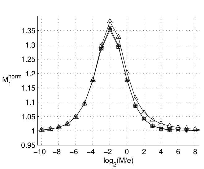
Fig. 1: The results of the calculation of the mass $M_{1}$ of lowest bound state at $\hat{\theta}=\theta=0$; $*$ corresponds to results, obtained by the extrapolation to the domain $K\to\infty$, $\bigtriangleup$ corresponds to $N=30$, $\square$ corresponds to known results of the calculation [9] on the lattice.

We have found good agreement [8] with lattice calculations in Lorentz coordinates for $\theta=0$ at any $M/e$, see fig. 1, and for $\theta=\pi$ at small $M/e$ (for larger $M/e$ we see the behaviour of the spectrum, indicating possible phase transition, that is seen also in mentioned lattice calculations), see fig. 2. On the fig. 1 we use normalized value

$$\halign{\hbox to\displaywidth{$\hfil\displaystyle#\hfil$}\cr 0.0pt{\hfil$\displaystyle\hskip 10.00002pt minus 10.00002ptM^{\rm norm}_{1}=\frac{M_{1}}{\sqrt{m^{2}+(2M)^{2}}},\hfil\hskip 10.00002pt minus 10.00002pt(28)\hfilneg\crcr}}$$

where $M_{1}$ is the mass of lowest bound state.

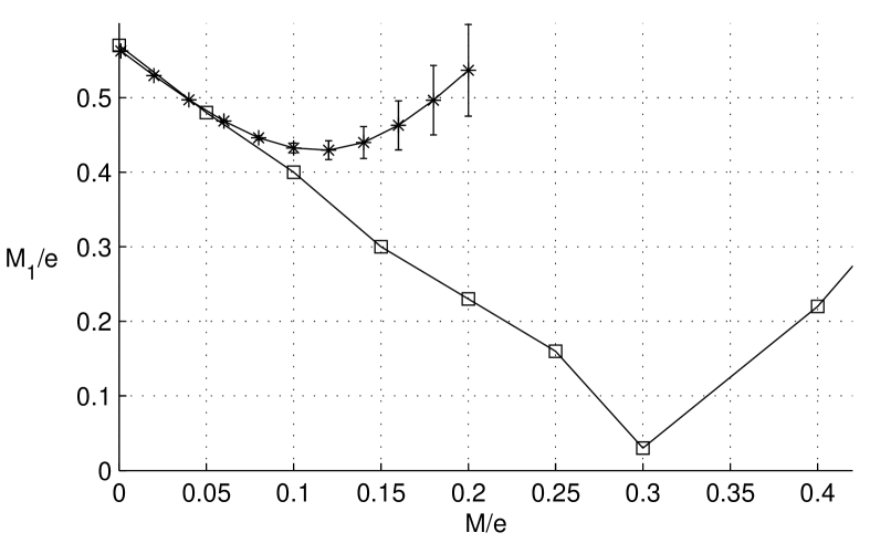
Fig. 2: The results of the calculation of the mass $M_{1}$ of lowest bound state at $\hat{\theta}=\theta=\pi$; $*$ corresponds to results, obtained by the extrapolation to the domain $K\to\infty$, $\square$ corresponds to known results of the calculation [10] on the lattice.

Beside of that we have calculated the spectrum for any other values of the parameter $\hat{\theta}$ (or for $0<\theta<\pi$) that was not yet done with lattice in Lorentz coordinates. We have found for all nonzero $\hat{\theta}$ some ”critical” region of $M/e$ where the mass spectrum becomes unbounded from the bottom. This indicates that the perturbation theory in $M/e$, that we used in our analysis, fails at these ”critical” values of $M/e$.

It is very interesting problem to find a way to continue our LF Hamiltonian to ”nonperturbative” in $M/e$ region.

Let us consider only LF Hamiltonian obtained perturbatively to all orders in $M/e$. We can formally find some Lagrangian, that generates this Hamiltonian via canonical formulation on the LF. Assuming that this Lagrangian is the ordinary one plus some counterterms, it is easy to find that these counterterms must be such that only the constraint, which connects $\psi_{-}$ and $\psi_{+}$ components of bispinor field $\psi=\left({\psi_{+}\atop\psi_{-}}\right)$, should be modified. In naive canonical formulation of QED(1+1 ) on the LF such constraint has the following form:

$$\halign{\hbox to\displaywidth{$\hfil\displaystyle#\hfil$}\cr 0.0pt{\hfil$\displaystyle\hskip 10.00002pt minus 10.00002pt\sqrt{2}\,\partial_{-}\psi_{-}-M\psi_{+}=0\hfil\hskip 10.00002pt minus 10.00002pt(29)\hfilneg\crcr}}$$

being the one of components of Dirac equation. ”Zero” mode of the $\psi_{-}$ is unconstrainted by this equation.

For our DLCQ formulation with antiperiodic in $x^{-}$ fields $\psi$ we introduce the following modification of this constraint :

$$\halign{\hbox to\displaywidth{$\hfil\displaystyle#\hfil$}\cr 0.0pt{\hfil$\displaystyle\hskip 10.00002pt minus 10.00002pt\sqrt{2}\,\partial_{-}\psi_{-}-M\psi_{+}+\frac{e\>e^{C}}{2\pi^{3/2}}e^{i(\omega-\hat{\theta})+i\frac{\pi}{2L}x^{-}}=0.\hfil\hskip 10.00002pt minus 10.00002pt(30)\hfilneg\crcr}}$$

Here the $\psi_{-}$ has no zero mode because of antiperiodic boundary conditions.

Now one can construct modified QED(1+1) Lagrangian, that generates this form of the constraint. Having such a Lagrangian one can construct corresponding LF Hamiltonian and substitute the solution of the constraint w.r.t. the $\psi_{-}$ into this LF Hamiltonian. In this way we come back to abovementioned form of corrected LF Hamiltonian.

The expression for the $\psi_{-}$, respecting our modified constraint, includes the operator $e^{i\omega}$. Taking into account the properties of this operator, we can check that correct values of vacuum condensate parameters, can be get on the LF using LF vacuum $|0\rangle$ for corresponding VEVs:

$$\halign{\hbox to\displaywidth{$\hfil\displaystyle#\hfil$}\cr 0.0pt{\hfil$\displaystyle\hskip 10.00002pt minus 10.00002pt\left.\langle 0|{\psi_{-}}^{+}\psi_{+}|0\rangle\right|_{M\to 0}=\left.\langle 0|\frac{1}{\sqrt{2}}\,\partial_{-}^{-1}\left(M{\psi_{+}}^{+}-\frac{e\,e^{C}}{2\pi^{3/2}}e^{-i(\omega-\hat{\theta})-i\frac{\pi}{2L}x^{-}}\right)\psi_{+}|0\rangle\right|_{M\to 0}\!\!\!=\frac{ee^{C}e^{i\hat{\theta}}}{2\pi^{3/2}}.\hfil\hskip 10.00002pt minus 10.00002pt(31)\hfilneg\crcr}}$$

3. A description of vacuum condensate in QCD on the LF

The remark at the end of previous section implies a possible way of semiphenomenological introduction of vacuum parameters in QCD(3+1) on the LF.

Namely, we can assume similar modification of the (3+1)-dimensional analog of the constraint equation, relating the $\psi_{-}$ and the $\psi_{+}$ on the LF, using the same DLCQ formulation. To make this correctly one has to introduce a lattice with respect to transverse coordinates. Here we only describe the idea. We introduce (3+1)-dimensional analog of operators $e^{i\omega}$ and $Q$, defining for each component of quark field $\psi_{j}(x)$ some unitary operator $U_{j}(x^{\bot})$ and ”transverse charges” $Q_{j}(x^{\bot})$. We require

$$\halign{\hbox to\displaywidth{$\hfil\displaystyle#\hfil$}\cr 0.0pt{\hfil$\displaystyle\hskip 10.00002pt minus 10.00002ptU_{j}(x^{\bot})\psi_{j}(x){U_{j}}^{+}(x^{\bot})=e^{i\frac{\pi}{L}x^{-}}\psi_{j}(x).\hfil\hskip 10.00002pt minus 10.00002pt(32)\hfilneg\crcr}}$$

Beside of that

$$\halign{\hbox to\displaywidth{$\hfil\displaystyle#\hfil$}\cr 0.0pt{\hfil$\displaystyle\hskip 10.00002pt minus 10.00002pt[U_{j}(x^{\bot}),Q_{j^{\prime}}({x^{\prime}}^{\bot})]=\delta_{jj^{\prime}}\delta_{x^{\bot}{x^{\prime}}^{\bot}}U_{j}(x^{\bot}),\cr 0.0pt{\hfil$\displaystyle Q_{j}(x^{\bot})|0\rangle=0,\cr 0.0pt{\hfil$\displaystyle U_{j}(x^{\bot})|0\rangle=d_{0j}^{+}(x^{\bot})|0\rangle,\cr 0.0pt{\hfil$\displaystyle U_{j}^{+}(x^{\bot})|0\rangle=b_{1j}^{+}(x^{\bot})|0\rangle.\hfil\hskip 10.00002pt minus 10.00002pt(33)\hfilneg\crcr}}}}}$$

Then we can write the component of Dirac equation that presents our LF constraint as follows:

$$\halign{\hbox to\displaywidth{$\hfil\displaystyle#\hfil$}\cr 0.0pt{\hfil$\displaystyle\hskip 10.00002pt minus 10.00002pt\sqrt{2}\,\partial_{-}\psi_{-j}(x^{\bot})+(\hat{D}_{\bot}-M)\psi_{+j}+\varkappa U_{j}(x^{\bot})e^{i\frac{\pi}{2L}x^{-}}=0,\hfil\hskip 10.00002pt minus 10.00002pt(34)\hfilneg\crcr}}$$

where

$$\halign{\hbox to\displaywidth{$\hfil\displaystyle#\hfil$}\cr 0.0pt{\hfil$\displaystyle\hskip 10.00002pt minus 10.00002pt\hat{D}_{\bot}=\sum_{k=1,2}\sigma_{k}D_{k},\hfil\hskip 10.00002pt minus 10.00002pt(35)\hfilneg\crcr}}$$

and the $\varkappa$ is a parameter related with possible vacuum effects. Resolving this constraint w.r.t. $\psi_{-j}$ we can obtain modified form of the QCD LF Hamiltonian, including vacuum parameter $\varkappa$, and consider bound state problem with this Hamiltonian.

First results on this way were discussed by S. Dalley and G. McCartor [11]. They showed that new terms influence the $q\bar{q}$ meson mass spectrum, correctly splitting masses of $\pi$ and $\rho$ mesons.

Acknowledgments. This work was supported by Russian Federal Education Agency, Grant No. RNP.2.1.1.1112, and President of Russian Federation, Grant No. NS-5538.2006.2. The work was supported also in part (S. A. P. and E. V. P.) by the Russian Foundation for Basic Research, Grant No. 05-02-17477.

References

[1]P. A. M. Dirac. Rev. Mod. Phys. 1949. V. 21. P. 392.
[2]V. A. Franke, Yu. V. Novozhilov, E. V. Prokhvatilov.
Lett. Math. Phys. 1981. V. 5. P. 239.
[3]V. A. Franke, Yu. V. Novozhilov, E. V. Prokhvatilov.
Lett. Math. Phys. 1981. V. 5. P. 437.
[4]M. Burkardt, A. Langnau.
Phis. Rev. D44 (1991) 1187, 3857.
[5]S. A. Paston, V. A. Franke.
Theor. Math. Phys. 1997. V. 112. P. 1117. hep-th/9901110.
[6]G. Dvali, R. Jackiw, S.Y. Pi.
Phys.Rev.Lett. 96 (2006) 081602.
[7]S. A. Paston, E. V. Prokhvatilov, V. A. Franke.
Theor. Math. Phys. 2002. V. 131. P. 516. hep-th/0302016.
[8]S. A. Paston, E. V. Prokhvatilov, V. A. Franke.
Phys. Atomic Nucl. 2005. V. 68. P. 67. hep-th/0501186.