Topological structure of the many vortices solution in Jackiw-Pi model

Abstract

By using the gauge potential decomposition, we discuss the self-dual equation and its solution in Jackiw-Pi model. We obtain a new concrete self-dual equation and find relationship between Chern-Simons vortices solution and topological number which is determined by Hopf indices and Brouwer degrees of $\Psi$-mapping. To show the meaning of topological number we give several figures with different topological numbers. In order to investigate the topological properties of many vortices, we use $5$ parameters(two positions, one scale, one phase per vortex and one charge of each vortex) to describe each vortex in many vortices solutions in Jackiw-Pi model. For many vortices, we give three figures with different topological numbers to show the effect of the charge on the many vortices solutions. We also study the quantization of flux of those vortices related to the topological numbers in this case.

I introduction

Chern-Simons theories based on secondary characteristic classes discovered in Ref.cs01 exhibit many interesting and important physical properties. In the early 1980, the first physical applications of the Chern-Simons form called topologically massive gauge theory was advanced by J. Schonfeldho01 , and many topological invariants of knots and links discovered in the 1980s could be reinterpreted as correlation functions of Wilson loop operators in Chern-Simons theorywt03 . Moreover, for gauge theories and gravity in three-dimensions, they can appeared as natural mass terms and will lead to a quantized coupling constant as well as a mass after quantizationdj02 . They have also found applications to a lot of physical problems, such as particle physics, quantum Hall effect, quantum gravity and string theoryykf ; ba98 ; jp01 ; re01 ; qh01 ; re02 ; re03 ; re04 ; re05 ; wt01 ; wt02 . Chern-Simons term acquire dynamics via coupling to other fieldsah01 ; ba98 , and get multifarious gauge theory, non-relativistic Chern-Simons theory supports vortices solutions, these static solutions can be obtained when their Hamiltonian was minimal. Vortices and their dynamics are interesting objects to be studiedah01 ; pd02 ; pd23 ; pd33 ; pd43 ; duth . R. Jackiw and S-Y. Pi considered a gauged, nonliner Schödinger equation in two spatial dimensions, with describes non-relativistic matter interacting with Chern-Simons gauge fields. Then they find explicit static, self-dual solutions which satisfies the Liouville equation and got an $n$-solitons solutions depends on $4n$ parameters(two positions, one scale, one phase per solition)ba98 ; jp01 . P. A. Horv$\acute{\mathrm{a}}$thy proved that the solution depends on $4N$ parameters without the use of an index theorem and the flux quantizationpa01 , and indicated the regular solutions with finite degree only arise for rational functions, the topological degree of those solutions is the common number of their zeros and poles on the Riemann spherepa02 .

In this paper, by using the gauge potential decompositiondg01 ; du01 ; sa01 ; li04 ; li05 , we will discuss topological structure of the self-dual solution in Jackiw-Pi model. We will look for complete many vortices solution from the self-dual equation and set up the relationship between the many vortices solution and topological number which is determined by Hopf indices and Brouwer degrees. We will give several figures to show the effects of the topological number on vortices. We also study the quantization of the flux of those vortices.

II the topological number of Self-dual vortex in Jackiw-Pi Model

In this section, based on the self-dual equation, we will look for complete vortex solution in Jackiw-Pi modelba98 making use of the decomposition of gauge potential. The Abelian Jackiw-Pi model in nonlinear Schrödinger systems isba98 ; jp01

$$\pounds_{jp}=\frac{k}{2}\epsilon^{\mu\nu\lambda}A_{\mu}\partial_{\nu}A_{\lambda}+i\hbar\Psi^{*}D_{0}\Psi-\frac{\hbar^{2}}{2m}|\mathbf{D}\Psi|^{2}+\frac{g}{2}(\Psi^{*}\Psi)^{2}.$$ (1)

[Here relativistic notation with the metric diag is (1,-1,-1) and $x^{\mu}=(ct,\mathbf{r})$.] Where $\mathbf{D}=\mathbf{\nabla}-i\frac{e}{\hbar c}\mathbf{A}$ and $\Psi$ is ”matter” field, the first term is the Chern-Simons density, which is not gauge invariant. Also $m$ is the mass parameter, $A_{\mu}$ is gauge potentials, $g$ governs the strength of nonlinearity, $\kappa$ controls the Chern-Simons addition and provides a cutoff at large distance greater than $\frac{1}{\kappa}$ for gauge-invariant electric and magnetic fields, which can be written as $\mathbf{E}=-\nabla\mathbf{A}^{0}-(\frac{1}{c})\partial_{t}\mathbf{A}$, and $\mathbf{B}=\mathbf{\nabla}\times\mathbf{A}$. Thus the Chern-Simons terms gives rise to massive, yet gauge-invariant ”electrodynamics”. The last term represents a self-coupling contact term of the type commonly found in nonlinear Schr odinger systems. The magnetic fields $B$ satisfies

$$B=\epsilon^{ij}\partial_{i}A^{j}=-\frac{e}{k}\rho,$$ (2)

where

$$\rho=\Psi^{*}\Psi,$$ (3)

with $g=\mp\frac{e^{2}\hbar}{mck}$, and sufficiently well-behaved fields so that the integral over all space of $\nabla\times\mathbf{J}$ vanishes, the energy is

$$H=\int d\mathbf{r}\mathcal{H}=\frac{\hbar^{2}}{2m}\int d\mathbf{r}|(D_{1}\pm iD_{2})\Psi|^{2}.$$ (4)

This is non-negative and vanishes. So it is obvious that $\Psi$ satisfies a self-dual equation

$$D_{1}\Psi=\mp iD_{2}\Psi.$$ (5)

To solve Eq.(5),we note that when $\Psi$ is decomposed into two scalar fields

$$\Psi=\Psi_{1}+i\Psi_{2}.$$ (6)

We can define a unit vector field $\mathbf{n}$ as follows

$$n^{a}=\frac{\Psi_{a}}{(\Psi^{*}\Psi)^{\frac{1}{2}}},a=1,2.$$ (7)

It is easy to prove that $\mathbf{n}$ satisfies the constraint conditions

$$n^{a}n^{a}=1,n^{a}dn^{a}=0.$$ (8)

From Eq.(5), and making use of the decomposition of U(1) gauge potential in terms of the two-dimensional unit vector field $\mathbf{n}$li05 , we can obtain

$$A^{i}=\frac{\hbar c}{e}(\epsilon^{ab}n^{a}\partial_{i}n^{b}\pm\frac{1}{2}\epsilon^{ij}\partial_{j}\ln\rho).$$ (9)

From Eq.(2) and Eq.(9) we get

$$B=\frac{\hbar c}{e}\epsilon^{ij}\epsilon^{ab}\partial_{i}n^{a}\partial_{j}n^{b}\pm\frac{\hbar c}{2e}\nabla^{2}\ln\rho,$$ (10)

i.e.

$$-\frac{e}{k}\rho=\frac{\hbar c}{e}\epsilon^{ij}\epsilon^{ab}\partial_{i}n^{a}\partial_{j}n^{b}\pm\frac{\hbar c}{2e}\nabla^{2}\ln\rho.$$ (11)

This equation can be rewritten as

$$\nabla^{2}\ln\rho=\pm\frac{2e^{2}}{\hbar ck}\rho\pm 2\epsilon^{ij}\epsilon^{ab}\partial_{i}n^{a}\partial_{j}n^{b},$$ (12)

with the help of the $\phi$ -mapping methoddu01 ; sa01 , Eq.(12) can be written as

$$\nabla^{2}\ln\rho=\pm\frac{2e^{2}}{\hbar ck}\rho\pm 4\pi\delta^{2}(\mathbf{\Psi})J\left(\frac{\mathbf{\Psi}}{\mathbf{r}}\right),$$ (13)

in which the vector field $\mathbf{\Psi}$ is defined by $\mathbf{\Psi}=(\Psi_{1},\Psi_{2})$, and $J\left(\frac{\mathbf{\Psi}}{\mathbf{r}}\right)$ is Jacobian

$$J\left(\frac{\mathbf{\Psi}}{\mathbf{r}}\right)=\frac{1}{2}\epsilon^{ab}\epsilon^{ij}\frac{\partial\Psi_{a}}{\partial x^{i}}\frac{\partial\Psi_{b}}{\partial x^{j}},i,j=1,2.$$ (14)

When $\rho\neq 0$, Eq.(13) will be the Liouville equation,

$$\nabla^{2}\ln\rho=\pm\frac{2e^{2}}{\hbar ck}\rho,$$ (15)

as we all know, the Eq.(15) has the general real solution as follows

$$\rho(\mathbf{r})=\frac{4\hbar c\kappa}{e^{2}}\frac{|f^{{}^{\prime}}(z)|^{2}}{[1+|f(z)|^{2}]^{2}},$$ (16)

in which

$$\mathbf{r}=(r\cos\theta,r\sin\theta),$$ (17)

where$z=re^{i\theta}$ and $f(z)$ is an arbitrary functionba98 .

Because $\rho$ is the charge density of the vortex, it must be positive, the Liouville equation is

$$\nabla^{2}\ln\rho=-\frac{2e^{2}}{\hbar c|\kappa|}\rho,$$ (18)

so the Eq.(16) should be

$$\rho(\mathbf{r})=\frac{4\hbar c|\kappa|}{e^{2}}\frac{|f^{{}^{\prime}}(z)|^{2}}{[1+|f(z)|^{2}]^{2}},$$ (19)

and the Eq.(13) can rewritten as

$$\nabla^{2}\ln\rho=-\frac{2e^{2}}{\hbar c|\kappa|}\rho-(sgn\kappa)4\pi\delta^{2}(\mathbf{\Psi})J\left(\frac{\mathbf{\Psi}}{\mathbf{r}}\right).$$ (20)

It is a Liouville equation with a $\delta-$function on its right side. For $\mathbf{r}=0$,this equation is also right. To show the meaning of the $\delta-$function of this equation, we will integrate Eq.(20) in section $III$, and discuss its singular point. For one vortex

$$f(z)=\left(\frac{c}{z-z_{0}}\right)^{N},$$ (21)

in which $c=r_{c}e^{i\theta_{c}}$ and $z_{0}=r_{0}e^{i\theta_{0}}$ is a complex constant, so there are $5$ real parameters involved in this solution : $2$ real parameters $z_{0}$ describing the locations of the vortices, $2$ real parameters $c$ corresponding to the scale and phase of each vortex, $1$ real parameters $N$ describing the charge of the vortex, and it is easy to obtain the radially symmetric solutionswe01

$$\rho=\frac{\hbar c}{e^{2}}{4|\kappa|N^{2}\over r_{c}^{2}}{\left(\frac{r-r_{0}}{r_{c}}\right)^{2N-2}\over\left(1+\left(\frac{r-r_{0}}{r_{c}}\right)^{2N}\right)^{2}},$$ (22)

where

$$N=-\frac{\kappa}{|\kappa|}Q+1$$ (23)

$$Q=\beta\eta,$$ (24)

where $Q$ is topological number of the vortex, those number is determined by Hopf indices and Brower degree of $\Psi$. Particularly, $\rho$ is invariant when change $N$ to $-N$, see Figure [1] and Figure [2] for a plot of the one vortex case, in this case, the center of the vortex is $z_{0}=3+3i$. In order to study the shape of the vortex, we slice off Figure[2] through it’s center, and define the hight and radius of the vortex, as is shown in Figure[3], we can obtain

$$r_{v}=r_{c}\left(1-\frac{2}{-\frac{\kappa}{|\kappa|}Q+1}\right)^{\frac{1}{-2\frac{\kappa}{|\kappa|}Q+2}}.$$ (25)

Figure [5] shows the values of the radius of the vortex as $Q$ is varied.

The height of the vortex

$$\rho_{max}=\frac{\hbar c|\kappa|}{r_{c}^{2}e^{2}}\left(\frac{\frac{\kappa}{|\kappa|}Q}{\frac{\kappa}{|\kappa|}Q-2}\right)^{\frac{1}{\frac{\kappa}{|\kappa|}Q-1}}\left(\left(\frac{\kappa}{|\kappa|}Q-1\right)^{2}-1\right).$$ (26)

Figure [4] shows the values of the height of the vortex as $Q$ is varied.

III the topological structure of the many vortices solution and their magnetic flux

In this section, making use of Eq.(20), we will discuss the topological structure of the many vortices solution, then we will study the magnetic flux of the vortices. The meromorphic function $f(z)$ yields a regular many vortices solution with finite magnetic flux if and only if $f(z)$ is a rational function,

$$f(z)=\frac{P(z)}{T(z)},$$ (27)

subject to

$$degP<degT.$$ (28)

In particular, when all roots of $T(z)$ are simple, $f(z)$ can be developed in to partial fractionspa01 ,

$$f(z)=\sum_{a=1}^{M}\frac{c_{a}}{z-z_{a}},$$ (29)

in which

$$z_{a}=r_{a}e^{i\theta_{a}},c_{a}=r_{0a}e^{i\theta_{0a}},a=1,2,...M.$$ (30)

So there are $4M$ real parameters involved in this solution : $2M$ real parameters $r_{a}$ and $\theta_{a}$ describing the locations of the vortices, $2M$ real parameters $r_{0a}$ and $\theta_{0a}$ corresponding to the scale and phase of each vortex. However, there is non evidence to believe the charge of each vortex equals to $1$, in order to study the charge and topological structure of each vortex in this solution, we suppose the charge of vortex $z_{a}$ is $N_{a}$(vortex $z_{a}$ is the vortex whose center is $z_{a}$), the we can rewrite $f(z)$ as

$$f(z)=\sum_{a=1}^{M}\left(\frac{c_{a}}{z-z_{a}}\right)^{N_{a}},$$ (31)

this describing $M$ separated $charge-N_{a}$ vortices, and $N_{a}>0$ because of $degP<degT$, then we add $M$ real parameters $N_{a}$ in our solution, these parameters describing the charge of each vortex and in the following text we will see that $N_{a}$ is relates to the topological number of each vortex.

Under the radially symmetric, $\nabla^{2}\ln\rho$ can be expressed as

$$\nabla^{2}\ln\rho=\frac{\partial^{2}}{\partial^{2}r}\ln\rho+\frac{1}{r}\partial_{r}\ln\rho.$$ (32)

Integrating Eq.(20)

$$\int\nabla^{2}\ln\rho d\mathbf{r}=\int\left[-\frac{2e^{2}}{\hbar c|\kappa|}\rho-(sgn\kappa)4\pi\delta^{2}(\mathbf{\Psi})J\left(\frac{\mathbf{\Psi}}{\mathbf{r}}\right)\right]d\mathbf{r}.$$ (33)

The Eq.(33) can be rewritten as

$$\int_{\mathbf{r}_{a}}^{\mathbf{r}_{a}+\mathbf{r}_{\epsilon}}\nabla^{2}\ln\rho d\mathbf{r}=-(sgn\kappa)4\pi\int_{\mathbf{r}_{a}}^{\mathbf{r}_{a}+\mathbf{r}_{\epsilon}}\delta^{2}(\mathbf{\Psi})J\left(\frac{\mathbf{\Psi}}{\mathbf{r}}\right)d\mathbf{r},$$ (34)

where $\mathbf{r}_{\epsilon}=(r_{\epsilon}\cos\theta,r_{\epsilon}\sin\theta),0\leq\theta\leq 2\pi$, and $r_{\epsilon}$ is a infinitesimal scalar, so $\int_{\mathbf{r}_{a}}^{\mathbf{r}_{a}+\mathbf{r}_{\epsilon}}$ is an integral in the infinitesimal region neighbouring the $\mathbf{r}_{a}$ point. The left side of this equation is

$$\int_{\mathbf{r}_{a}}^{\mathbf{r}_{a}+\mathbf{r}_{\epsilon}}\nabla^{2}\ln\rho d\mathbf{r}=4\pi(N_{a}-1).$$ (35)

Suppose that the vector field $\Psi^{a}$ possess $M$ isolated zeros which is in $\mathbf{r}=\mathbf{r}_{a}$, according to the $\delta$-function theorydelt , $\delta^{2}(\mathbf{\Psi})$ can be expressed by

$$\delta^{2}(\mathbf{\Psi})=\sum_{a=1}^{M}\frac{\beta_{a}}{\mid J\left(\frac{\mathbf{\Psi}}{\mathbf{r}}\right)\mid_{\mathbf{r}=\mathbf{r}_{a}}}\delta^{2}(\mathbf{r}-\mathbf{r}_{a}),$$ (36)

and then we can obtain

$$\int_{\mathbf{r}_{a}}^{\mathbf{r}_{a}+\mathbf{r}_{\epsilon}}4\pi\delta^{2}(\mathbf{\Psi})J\left(\frac{\mathbf{\Psi}}{\mathbf{r}}\right)d\mathbf{r}=4\pi\int_{\mathbf{r}_{a}}^{\mathbf{r}_{a}+\mathbf{r}_{\epsilon}}\beta_{a}\eta_{a}\delta^{2}(\mathbf{r}-\mathbf{r}_{a})d\mathbf{r},$$ (37)

where $\beta_{a}$ is positive integer (the Hopf index of the zero point) and $\eta_{a}$, the Brouwer degree of the vector field $\mathbf{\Psi}$,

$$\eta_{a}=sgnJ\left(\frac{\mathbf{\Psi}}{\mathbf{r}}\right)|_{\mathbf{r}=\mathbf{r}_{a}}=\pm 1.$$ (38)

The meaning of the Hopf index $\beta$ is that while $\mathbf{r}$ covers the region neighbouring the $z_{a}$ point once, the vector field $\mathbf{\Psi}$ covers the corresponding region $\beta_{a}$ times. Hence, $\beta_{a}$ and $\eta_{a}$ are the topological number which shows the topological properties of the vortex solution. We have

$$\delta^{2}(\mathbf{\Psi})J\left(\frac{\mathbf{\Psi}}{\mathbf{r}}\right)=\beta_{a}\eta_{a}\delta^{2}(\mathbf{r}-\mathbf{r}_{a}).$$ (39)

If we define the topological number $Q_{a}$ of the vortex whose center is $z_{a}$ as

$$Q_{a}=\int_{\mathbf{r}_{a}}^{\mathbf{r}_{a}+\mathbf{r}_{\epsilon}}\delta^{2}(\mathbf{\Psi})J\left(\frac{\mathbf{\Psi}}{\mathbf{r}}\right)d\mathbf{r}=\beta_{a}\eta_{a},$$ (40)

from Eq.(34) we can get

$$N_{a}-1=-(sgn\kappa)Q_{a},$$ (41)

in which $N_{a}-1\geq 0$, so $\kappa$ must satisfied $sgn\kappa=-sgnJ$ and we can set $-(sgn\kappa)Q_{a}=|Q_{a}|$, then the total charge of those vortices

$$N=degT=\sum_{a=1}^{M}N_{a}=\sum_{a=1}^{M}|Q_{a}|+M=-(sgn\kappa)Q+M,$$ (42)

in which $Q$ is the total topological number which can be defined as

$$Q=\sum_{a=1}^{M}Q_{a}.$$ (43)

Substituting Eq.(41) into Eq.(31), we can obtain

$$f(z)=\sum_{a=1}^{M}\left(\frac{c_{a}}{z-z_{a}}\right)^{|Q_{a}|+1},$$ (44)

it is obviously that Eq.(44) and Eq.(19)is the solution of Eq.(20). On the other hand, this means vortices density $\rho$ relates to its topological number $Q_{a}=\beta_{a}\eta_{a}$. We now see that $N_{a}$ must be an integer.

We can see the point $r_{a}$ is a singular point of the field $\mathbf{\Psi}$, and it is non-degenerate. In our case, we can list the possible four types of non-degenerate singular points in two dimensionsbook :

$1)$a center with index $1$(when both eigenvalues are purely imaginary);

$2)$a node with index $1$(eigenvalues real and the same sign);

$3)$a focal point index $1$(complex conjugate eigenvalues, not purely imaginary);

$4)$a saddle point of index $-1$(eigenvalues real and the opposite sign).

Information about singular piont of a vector field is of grate importance for obtaining a qualitative picture of the behavior of the integral trajectories of the field.

If we note the unit magnetic flux $\Phi_{0}=\frac{2\pi\hbar c}{e}$, one can get

$$\int_{0}^{\infty}\mathbf{B}d\mathbf{r}=-(sgn\kappa)\frac{2Nhc}{e}=-2(sgn\kappa)\Phi_{0}\left[-(sgn\kappa)Q+M\right],$$ (45)

from this equation we know the magnetic flux is quantized. When the total topological number equal to zero, the magnetic flux of this vortex is

$$\Phi=\int_{0}^{\infty}\mathbf{B}d\mathbf{r}=-2(sgn\kappa)M\Phi_{0}.$$ (46)

For example, when set $M=1$ in Eq.(31), we can get the one vortex solution Eqs.(22). When set $M=2$ in Eq.(31), we can get the two vortices solution with $z_{1}=-3,z_{2}=3,c_{1}=c_{2}=1$, i.e.

$$f(z)=\left(\frac{1}{z+3}\right)^{|Q_{1}|+1}+\left(\frac{1}{z-3}\right)^{|Q_{2}|+1},$$ (47)

with Eq.(19), we can give the solution of two vortices. See Figure [4] for a plot of the two vortex case.

When set $M=3$ in Eq.(31), we can get the three vortices solution with $z_{1}=-3-\sqrt{3}i,z_{2}=3-\sqrt{3}i,z_{3}=2\sqrt{3}i,c_{1}=c_{2}=c_{3}=1$, it is as

$$f(z)=\left(\frac{1}{z-z_{1}}\right)^{|Q_{1}|+1}+\left(\frac{1}{z-z_{2}}\right)^{|Q_{2}|+1}+\left(\frac{1}{z-z_{3}}\right)^{|Q_{3}|+1},$$ (48)

with Eq.(19), we can obtain the solution of three vortices. See Figure [7] for a plot of the three vortices case and Figure[8] for the four vortices case. Note the ring-like form of the magnetic field for these Chern-Simons vortices, as the magnetic field is proportional to $\rho$, $\mathbf{B}$ vanishes where the field $\Psi$ vanishes. From those figures we can see the shape of those vortices is different when their topological numbers is different. So it is not enough to use $4M$ parameters to describe many vortices, we must induct a charge parameter $N$, from Figure[4] and Figure[5] we can see, the hight and radius of the vortex depends on $Q$.

IV Conclusions

In this paper, We discuss the self-dual equation and its solution in Jackiw-Pi model By using the gauge potential decomposition and $\Psi$-mapping method, we get a Liouville equation with a $\delta$ function, then we also obtain the solution of this equation, and the $\delta$ function will not change the character of the solution when $\rho\neq 0$. We add $M$ parameters to the $M$-vortices solution, those parameters describing the charge of each vortex, i.e. use $5M$ parameters(two positions, one scale, one phase per vortex and one charge per vortex) to describe $M$-vortices solutions in Jackiw-Pi model. We studied the topological structure of Chern-Simons vortices in Jakiw-Pi model by calculate the integral of the Liouville equation, and find the charges of those vortices are determined by the topological numbers of those vortices, those topological numbers are determined by Hopf indices and Brouwer degrees of $\Psi$-mapping, the total topological number of these vortices is conservational. We also give some figures with different topological numbers to show the relationship between the shape of those vortex and topological numbers. In many vortices solution, in order to show the shape of those vortices is different when only their topological number is different, we show some vortices only with different positions and different topological numbers in many vortices figures(see Figure[6];[7];[8]). We also find the relationship between the quantization of the flux and the topological numbers from the integral value of the solution in the whole space. However, the flux is non-vanish when the topological number equals to zero. So does the the angular momentum.

V acknowledgments

We thank professor P. A. Horv$\acute{\mathrm{a}}$thy for his important information. This work was supported by the CAS Knowledge Innovation Project (KJX2-SW-N16;KJCX3-SYW-N2) and Science Foundation of China (10435080, 10275123).

VI references

Figure 1: Density $\rho$ for solution (22) representing one vortex with $Q=0$.

Figure 2: Density $\rho$ for solution (22) representing one vortex with $Q=1$.

Figure 3: The section plane of Figure[2], this section plan includes the center of this vortex, as is shown in this figure, we can define the hight $\rho_{max}$ and radius $r_{v}$ of the vortex.

Figure 4: The values of the height of the vortex as $Q$ is varied$(\hbar=c=1)$.

Figure 5: The values of radius of the vortex as $Q$ is varied$(\hbar=c=1)$.

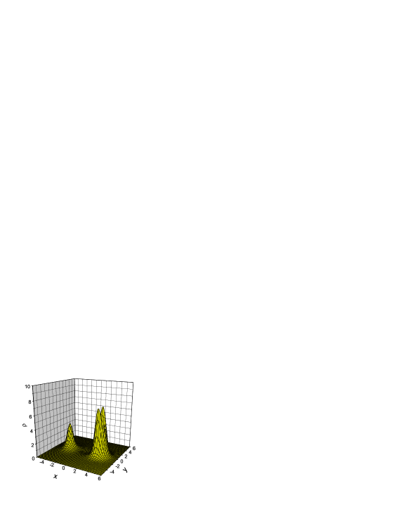
Figure 6: Density $\rho$ for solution (47) representing two separated vortices with $Q_{1}=0,Q_{2}=1$.

Figure 7: Density $\rho$ for solution (48) representing three separated vortices with $Q_{1}=0,Q_{2}=1,Q_{3}=2$.

Figure 8: Density $\rho$ representing four separated vortices with $Q_{1}=0,Q_{2}=1,Q_{3}=2,Q_{4}=3$.

References

- (1) S. S. Chern and J. Simons, Proc. Nat. Acad. Sci. USA 68(4), 791 (1971); S. S. Chern and J. Simon,Ann. Math. 99, 48 (1974).
- (2) J. Schonfeld, Nucl. Phys. B185, 157 (1981).
- (3) E. Witten, Commun. Math. Phys. 121, 351 (1989).
- (4) S. Deser, R. Jackiw and S. Templeton, Phys. Rev. Lett. 48, 975 (1982). S. Deser, R. Jackiw and S. Templeton, Ann. of Physics 140, 372 (1982).
- (5) R. Jackiw and E. J. Weinberg, Phys. Rev. Lett. 64, 2234 (1990).
- (6) R. Jackiw and S. Y. Pi, Phys. Rev. Lett. 64, 2969 (1990).
- (7) R. Jackiw and S. Y. Pi, Phys. Rev.D 42, 3500 (1990).
- (8) J. Hong, Y. Kim and P. Y. Pac, Phys. Rev. Lett. 64, 2230 (1990).
- (9) S. M. Girvin and A.H. MacDonald, Phys. Rev. Lett. 58, 1252 (1987).
- (10) S.C. Zhang, T.H. Hansson and S. Kivelson, Phys. Rev. Lett. 62, 82 (1988).
- (11) V. Kalmeyer and R. B. Laughlin, Phys. Rev. Lett. 59, 2095 (1987);
- (12) R. B. Laughlin, Phys. Rev. Lett. 60, 2677 (1988).
- (13) A. Achucarro and P.K. Townsend , Phys. Lett. B 180, 89 (1986) .
- (14) E. Witten, Chern CSimons gauge theory as a string theory, in: The Floer Memorial Volume, in: Progress in Mathematics, vol. 133, Birkhauser, Boston, MA, 1995, pp. 637 C678. arXiv:hep-th/9207094
- (15) E. Witten, Nucl. Phys. B 311, 46 (1988).
- (16) A. A. Abrikosov, Sov.Phys. JETP 5,1174(1957).
- (17) Bogomol nyi, E.B.: The stability of classical solutions. Sov. J. Nucl. Phys. 24, 449 (1976).
- (18) H. Nielsen and P. Olesen, Nucl. Phys. B 61, 45 (1973).
- (19) H. J. de Vega and F. A. Schaposnik, Phys. Rev. Lett.56, 2564 (1986); Phys. Rev. D 34, 3206(1986) .
- (20) N.Manton, Nucl. Phys. B 400, 624(1993).
- (21) Y. Q. Wang, T. Y. Si, Y. X. Liu and Y.S. Duan, Mod. Phys. Lett. A 20 3045(2005) [hep-th/0508111]
- (22) P. A. Horvthy, J.-C. Yera, Lett. Math. Phys. 46, 111-120 (1998) [hep-th/9805161].
- (23) P. A. Horvthy, Lett. Math. Phys. 49, 67-70 (1999) [hep-th/9903116].
- (24) Y. S. Duan, M. L. Ge, Sci. Sin. 11, 1072(1979); Y. S. Duan and X. H. Meng, J. Math.Phys. 34, 1149 (1993).
- (25) Y. S. Duan, G. H. Yang, and Y. Jiang, Gen. Rel. Grav. 29, 715 (1997)
- (26) Y. S. Duan: SALC-PUB-3301(1984).
- (27) Y. S. Duan and X. G. Lee, Helv.Phys.Acta. 58, 513 (1995).
- (28) X. G. Lee, M. Baldo and Y. S. Duan, Gen. Rel. Grav. 29, 715 (1997).
- (29) X. G. Lee, et. al. Commom. Theor. phys.(accepted).arxiv:hep-th/0604138
- (30) H. Hopf, Math. Ann. 96, 209 (1929).
- (31) A. S. Achwarz, Topology for Physicists. Springer-Verlag, Berlin,1994.
- (32) B. A. Dubrovin, A. T. Fomenko, S. P. Novikov, The Geometry and Toplogy of Manifolds.(Springer-Verlag, Berlin, 1985)