SNUTP-06-006
Intersecting Brane World
From Type I Compactification

Abstract

We elaborate that general intersecting brane models on orbifolds are obtained from type I string compactifications and their $T$-duals. Symmetry breaking and restoration occur via recombination and parallel separation of branes, preserving supersymmetry. The Ramond–Ramond tadpole cancelation and the toron quantization constrain the spectrum as a branching of the adjoints of $SO(32)$, up to orbifold projections. Since the recombination changes the gauge coupling, the single gauge coupling of type I could give rise to different coupling below the unification scale. This is due to the nonlocal properties of the Dirac–Born–Infeld action. The weak mixing angle $\sin^{2}\theta_{W}=3/8$ is naturally explained by embedding the quantum numbers to those of $SO(10)$.

Keywords: unification, intersecting branes, recombination, weak mixing angle.

1 Introduction

There are two nice descriptions of gauge theory from string theory, which we expect, in the end, to bring forth the Minimal Supersymmetric Standard Model (MSSM). One is a closed string on which the charge is distributed homogeneously and gives rise to the current algebra. This idea is realized by heterotic string, and by compactification on a suitable manifold, we obtain semi-realistic theories close to MSSM. The other is open string description of type I and type II strings. There the gauge degree of freedom, so called Chan–Paton factor, is assigned on the endpoints of open strings, whose modern understanding is provided by D-brane stacks, in the $T$-dual picture. In particular, the chiral fermions emerge on intersections of branes at angle [1]. This provides the framework of a collection of models called intersecting brane world [2].

The most unsatisfactory point of the brane picture has been the lack of understanding on unification, thus conventional models have resorted to bottom-up approach. However, if we consider string theory as the first principle from which we reduce our world, there must be unification. Then the theory is consistent by construction. For instance, anomaly cancelation is automatically satisfied if we spontaneously break an unified theory, which is anomaly free by nature. Also from the bottom, the running gauge couplings from MSSM and unification around $10^{16}$ GeV [3] is quite appealing. For the resulting low-energy vacua to be explained by spontaneous symmetry breaking, we should have an unified gauge group and coupling at the symmetry breaking scale. In this paper, we consider this possibility.

The Higgs mechanism via adjoint representation is easy to understand. The nonabelian gauge group is realized by a stack of coincident branes. Their positions are denoted by matrix-valued vector $X^{m}$ also transforms as an adjoint. When they are diagonal in group space, the geometric information on D-branes translates to that on the gauge setup. There it is a Wilson line

$$A_{m}={1\over 2\pi\alpha^{\prime}}X^{m}=\begin{pmatrix}a_{1}&&&\\ &a_{2}&&\\ &&\ddots&\\ &&&a_{n}\end{pmatrix},$$ (1)

where $1/(2\pi\alpha^{\prime})$ is the string tension. In general they represent a broken phase of $U(1)^{n}\subset U(n)$. When some elements are same, or some branes are coincident, the gauge symmetry is enhanced to $\prod U(n^{i})$, where $n^{i}$ is the number of the same elements. We can see that the symmetry breaking corresponds to brane separation. The parallel branes are half-Bogomoln’yi-Prasad-Sommerfield (BPS) system, thus parallel separation does not break further supersymmetries. Also the D-flatness is not spoiled since D-term potential is given by

$${\rm Tr\,}[X^{m},X^{n}]^{2}$$ (2)

from dualizing the gauge kinetic term.

However to explain the chiral nature of matter fermions, we need intersecting branes. Still in the intersecting case, the parallel separation moduli survive [4, 5]. However we have also a deformation between intersecting and parallel branes, known as recombination [6, 7, 8, 9, 10, 11, 12]. In the non-supersymmetric case, the instability is recovered by recombination, setteling down to minimal volume setup. However we see that if protected by supersymmetry, the recombination costs no energy.

In this paper we consider compactifications on orbifold with suitable orientifold planes. To have supersymmetric models, we require some “F-flatness” condition, which is a generalization of self-dual condition [13]. Also we have the Ramond–Ramond (RR) charge conservation, realized as tadpole cancelation condition, which guarantees the absence of anomalies. We will see that every configuration satisfying these have the same energy, in particular, to type I compactification on the same orbifold. Thus we naturally expect that also deformation along the flat directions could explain the spontaneous symmetry breaking of gauge group from type I compactification [6]. During the recombination, although the intersection points, hence local chiralities, are changed, but the charge is conserved thus the total amount of anomalies is not affected. These points are examined in section 3. Such unification picture is also natural from the charge embedding, as to be discussed in section 2 in the modern D-brane picture. From quantization condition for tilted branes, charges are embedded into adjoint representations, which then belong to those of $SO(32)$ and a bifundamental representations occur as off-diagonal entries of them, like the $X,Y$ bosons in Georgi–Glashow unification [14], for instance. In section 4, we analyze the gauge coupling unification using fluctuation spectrum analysis of Dirac–Born–Infeld (DBI) action [6, 15, 16]. Also we comment on the desirable weak mixing angle $\sin^{2}\theta=3/8$ at the unification scale.

2 Adjoint embedding

We begin with the proper description of intersecting branes by embedding representations into an adjoint of nonabelian group. Bifundamental representations can arise from branching of adjoints. They are the only possible representation from open strings.

2.1 Toron quantization

Toron is a quantum of constant magnetic field on the torus [18]. They are realized by various D-branes and their bound states.

Two dimensional case

Consider a D1-brane wrapping on a two torus $T^{2}$ in 12-directions. In string theory a torus $T^{2}$ as a target space is specified by two complex numbers, namely the complex structure $\tau$ and Kähler modulus $B+iA$ where $A=L^{2}{\rm Im\,}\tau,L\in{\bf R},\tau\in{\bf C}$ and $B$ is the NSNS antisymmetric tensor. It is equivalent to choice of basis vectors $e_{1}=L,e_{2}=L\tau$ and a NSNS field $B$. This D1-brane is specified by two integral numbers $(n,m)$, namely straightly winding $n,m$ times along $e_{1},e_{2}$ directions respectively. We easily see that the cycle is of the minimal length for given $(n,m)$ and described as

$$\frac{1}{2\pi\alpha^{\prime}}X^{2}=F_{12}X^{1}+A^{0}_{1},$$ (3)

where

$$\begin{split}F_{12}&={2\pi\over A}{m\over n}{\bf 1}_{n}\equiv\tan(g\theta){2\pi\over A}{\bf 1}_{n}\\ A^{0}_{1}&={2\pi\over A}\frac{1}{n}{\rm diag}(0,1,\dots,n-1)+c,\end{split}$$ (4)

with the string coupling $g$, the identity matrix of rank $n$ and a constant $c$. $\theta$ is interpreted as the relative angle to 1-direction. Although we have a single cycle, we employed matrix structure in the group space in the spirit of (1). We regard it as a single brane identified inside the torus, rather than $n$ slices of equally separated D-brane with permutation symmetry. This quantization arises by requiring closedness of the brane, since it can only end on other D or NS branes, not on the empty space. Although a homologous setup with $n$ parallel D1 branes along 1-direction and $m$ branes along 2-direction has the same charge, it is a different setup.

The gauge degree of freedom a fluctuation around this flux (3). Although embedded in $U(n)$, the actual degree of freedom is smaller $U(p)$ for $p\equiv\gcd(n,m)$. We can check that $p$ is the maximal effective number of coincident branes, easily seen from the geometric picture. In the gauge theory point of view, there can be at most $p$ permutation symmetry $S_{p}$ in (3). It also means, having less permutation symmetry, we can break the above $U(p)$ gauge group by parallel separation, adjusting constant matrix in (4) in analogy with the Wilson line case (1).

$T$-duality in 2-direction maps the two to D0 brane and D2 brane. Two moduli are exchanged and $L^{\prime}=2\pi\alpha^{\prime}/L$. The above becomes

$$A_{2}=F_{12}X^{1},\quad A_{1}=0,$$ (5)

which is a form of gauge fixed constant magnetic flux. From the rank of the matrix $n$ slices of D2 brane describe worldvolume $U(n)$ gauge theory. This is the consistent solution satisfying the ’t Hooft boundary condition [18, 15]. The condition (4) become quantization condition.

$$c_{1}=\frac{1}{2\pi}\int d^{2}x{\rm Tr\,}F_{12}=m,$$ (6)

with $m$ being integer, indeed, from vortex quantization. From the Chern–Simons coupling, the constant flux is interpreted as 0-brane charge  $i\mu_{2}2\pi\alpha^{\prime}\int_{T^{2}\times M}{\rm Tr\,}F_{12}\wedge C_{0}=im\mu_{0}\int_{M}C_{0}$ so we have $m$ D0-branes. This is interpreted as D0-D2 bound state and in fact D0 brane has melt into D2 brane, leaving the flux (5) on it. This bound state is again 1/2 BPS state [24].

By a series of $SL(2,{\bf Z})$-dual there is a configuration where we have $p$ zero branes only on $T^{2}$ with the moduli space $(T^{2})^{p}/S_{p}$ [20], thus we again see that the resulting gauge group is $U(p)$.

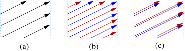
Figure 1: A cycle with winding number $(3,2)$ describes gauge group $U(1)$, as a broken phase of $U(3)$ due to the quantization condition (a). A $(6,4)$ cycle, a double copy of (3,2), generically has $U(1)\times U(1)\subset U(6)$ (b), and can be enhanced to $U(2)\subset U(6)$ when branes are coincident (c).

Note that $T$-dual in 12-direction, we exchange $n$ and $m$, i.e. we have $U(m)$ gauge symmetry with the first Chern number $n$. This symmetry is not visible in gauge theory since it only take into account K-theory charge, but natural in the sense it merely corresponds to exchanging coordinates $x^{1}$ and $x^{2}$. (In higher dimensional case, in the shrinking instanton limit, we see both gauge group.) Thus even if we have $U(1)$ gauge symmetry, the theory is naturally embedded in $U(n)$ or $U(m)$ gauge theory. In other words, the natural embedding is nonabelian.

A pair of parallel D1-branes can make further bound state between themselves, which is equivalent to one D1-brane winding twice the same cycle. The $SU(2)$ degree of freedom decouples and the low energy degree of freedom is $U(1)$ gauge theory [25]. For the above $(n,m)$ cycle, we see there is $p$ kinds of bound states. This bound state is not distinguishable, by the charge, or Chern number.

When we have more than one stacks in the same torus, we may generally have a number of cycles. The resulting toron background is expressed as

$$F_{12}={2\pi\over A}\begin{pmatrix}{m^{1}\over n^{1}}{\bf 1}_{n^{1}}&&\\ &\ddots&\\ &&{m^{k}\over n^{k}}{\bf 1}_{n^{k}}\end{pmatrix}.$$ (7)

Without loss of generality, we can make the setup that each block satisfies the above condition (6). However the important measure is the first Chern number $c_{1}=\sum_{1}^{k}m^{a}$. It seems natural to embed the field strengths of all the stacks into a single nonabelian one. Evidently, by the form of matrix, it is a Higgs phase of

$$U(n^{1})\times\cdots\times U(n^{k})\subset U(n),\quad n=\sum_{a=1}^{k}n^{a},$$ (8)

generalizing (1). Although this setup cannot directly come from the single stack (4), all of them can be regarded to reside specific points in moduli space of $U(n)$ gauge theory. This is clear in the bound state picture that we have $n$ D2- and $c_{1}$ D0-branes forming $k$ bunch of bound states. How differently they can bound determines the setup. Shortly we will see that there is an upper limit on $m$ and $n$ from the tadpole cancelation condition.

For general compactifications on ${\bf Z}_{N}$ or ${\bf Z}_{M}\times{\bf Z}_{N}$ orbifolds the unit torus is not rectangular but parallelogram with $\tau\neq 1$, to be compatible with orbifold group. This tilting is also required even if we can have rectangular tori, since intersection number accounting for the number of generations, is even in general, compared to the observed number, three. In a the case of our interest, worldsheet parity projection $\Omega$ projects out antisymmetric NSNS $B$ field. When we compactify it, $B$ field in the compact dimension can assume discretized, half-integral values $0,\frac{1}{2}$ modulo 1 [27, 28]. In the $T$-dual picture, this is the compatibility of orientifold action $\Omega R$ on torus, and ${\rm Re\,}\tau=0,\frac{1}{2}$ modulo 1. In the half-integral case, the RR charge of orientifold is reduced by half, which leads rank and multiplicity reduction. For the ${\rm Re\,}\tau=\frac{1}{2}$ case, it is convenient to define

$$\tilde{m}=m+\frac{1}{2}n.$$

In the literature, they are called A- and B-torus respectively. The angle condition is related to

$$\tan g\theta={m+n{\rm Re\,}\tau\over n{\rm Im\,}\tau}=\left\{\begin{matrix}\displaystyle{m\over n{\rm Im\,}\tau}&({\rm Re\,}\tau=0)\\ \\ \displaystyle{\tilde{m}\over n{\rm Im\,}\tau}&({\rm Re\,}\tau=\frac{1}{2})\end{matrix}\right..$$ (9)

Evidently, for the case of titled torus, the discussion is not changed if we replace a cycle number with a tilted one.

Four and higher dimensions

We can generalize the above idea to arbitrary dimensions. There are six two-cycles in four-torus, i.e. dim$\,H_{2}(T^{4},{\bf Z})=6$. They can also be represented by six integral numbers. In $T$-dual space, the system looks as D0-D4 bound states and the six numbers are related to Chern numbers

$$(N,c_{1}^{12},c_{1}^{34},c_{2},c^{14}_{1},c^{23}_{1}).$$ (10)

The $c_{i}$ denotes the $i$th Chern numbers in $T$-dual picture, where we have D0 and D4 branes and the superscript denotes the direction. These numbers can be reshuffled by $T$-dualities $SL(4,{\bf Z})$, and with it we may make three of them to be zero [19, 53]. For convenience we will consider the factorizable cycle $Nc_{2}=c_{1}^{12}c_{1}^{34},c_{1}^{14}=0$, which is understood as that of direct product of two-torus. However, the discussion will not be changed for the non-factorizable cycle. The cycles are denoted by three independent numbers

$$(n_{1},m_{1})(n_{2},m_{2})=(n_{1}n_{2},n_{1}m_{2},m_{1}n_{2},m_{1}m_{2})=(N,c_{1}^{14},c_{1}^{23},c_{2}).$$ (11)

Therefore we have

$$F_{12}={2\pi\over A_{1}}\begin{pmatrix}{m^{1}_{1}\over n^{1}_{1}}{\bf 1}_{N^{1}}&&\\ &\ddots&\\ &&{m^{k}_{1}\over n^{k}_{1}}{\bf 1}_{N^{k}}\end{pmatrix},\quad F_{34}={2\pi\over A_{2}}\begin{pmatrix}{m^{1}_{2}\over n^{1}_{2}}{\bf 1}_{N^{1}}&&\\ &\ddots&\\ &&{m^{k}_{2}\over n^{k}_{2}}{\bf 1}_{N^{k}}\end{pmatrix}.$$ (12)

Beside the multicomponent in the different directions, only the slight different is that the rank of each unit matrix is now $N^{a}=n_{1}^{a}n_{2}^{a}$. The slopes stay in the same form, but now they can be also expressed by Chern numbers $m/n=c^{ij}_{1}/c_{2}$. Again, we see that the system is naturally embedded into $U(N)$ theory, where $N=\sum N^{a}$. Note that the quantization condition requires the dimensions of diagonal blocks to be the same $I_{N^{a}}$, although the slopes can be different. Each describes one stack of branes. Therefore, as in the parallel brane case, it seems natural and suggestive to embed all the branes into one representation and regard the subalgebra as a broken phase. We will see the upper limit of the rank will be given by tadpole cancelation condition.

For the six dimensional case, the factorizable three cycle is represented as

$$\begin{split}&(n_{1},m_{1})(n_{2},m_{2})(n_{3},m_{3})\\ &=(n_{1}n_{2}n_{3},n_{1}m_{2}m_{3},m_{1}n_{2}m_{3},m_{1}m_{2}n_{3},m_{1}m_{2}m_{3},m_{1}n_{2}n_{3},n_{1}m_{2}n_{3},n_{1}n_{2}m_{3})\\ &=(N,c^{12}_{2},c^{34}_{2},c^{56}_{2},c_{3},c_{1}^{12},c_{1}^{34},c_{1}^{56})\end{split}$$ (13)

We can straightforwardly generalize such toron descriptions to an arbitrary number of extra dimensions. In such descriptions, all the information is contained in the Chern numbers. As pointed out [29], these information can only take into account of K-theory charge, not the cohomological information. So brane and antibrane is not distinguishable, but only the charge difference does. In this sense, the description as (21) is far from complete. It cannot describe a brane lying vertically on the torus $n_{a}=0$ nor antibrane cycle $n_{a}<0$ and, more severely, when the off-diagonal component of (21) is turned on, the corresponding cycle is not same as $(n_{a},m_{a})$ any more, resulting in different magnetic flux. Measuring D-brane charge by cohomology rather than K-theory amounts to measuring a K-theory class by Chern classes.

2.2 Bifundamental representations

One noticed that, for example, the $X,Y$ gauge bosons in the conventional Georgi–Glasow $SU(5)$ unification [14] have the correct quantum numbers, i.e. colors and weak isospins $\bf(3,2)$, as (s)quarks. Of course they do not have the desired $U(1)$ hypercharges, but provided that they are also charged under additional $U(1)$ symmetries, after diagonal symmetry breaking they may have the correct quantum numbers. We see that such structure can explain the bifundamental representation of MSSM matters embedded into adjoint representations, which is the quantum number of a string stretched between branes localized at an intersection.

Consider a symmetry breaking $G=U(p^{a}+p^{b})\to H=U(p^{a})\times U(p^{b})$. The case with more $U(n)$ for $H$ is to be straightforwardly generalized by iteration. With a gauge choice we can take

$$A_{m}={2\pi\over A}\begin{pmatrix}\ddots&&&&\\ &\displaystyle{m^{a}\over n^{a}}{\bf 1}_{N^{a}}&\\ &&\ddots&\\ &&&\displaystyle{m^{b}\over n^{b}}{\bf 1}_{N^{b}}&\\ &&&&\ddots\end{pmatrix}X^{n}+A_{m}^{0}.$$ (14)

Naturally $p^{i}=\gcd(n^{i},m^{i})$. In $4k+2$ dimension, the Dirac spinor can be decomposed into two Weyl representations

$$\text{$/$ $\nabla$}=\begin{pmatrix}0&i\text{$/$ $\partial$}+A_{z}\\ i\bar{\text{$/$ $\partial$}}+A_{\bar{z}}&0\end{pmatrix},\quad\Psi(z,\bar{z})=\begin{pmatrix}\Psi_{+}\\ \Psi_{-}\end{pmatrix}.$$ (15)

Note that this kind of decomposition is possible when we have $4k+2$ extra dimensions. Under the above gauge group $H$, an adjoint fermion is naturally decomposed as

$$\quad\Psi_{\pm}=\begin{pmatrix}\ddots&&&&\\ &A_{\pm}&&B_{\pm}\\ &&\ddots&&\\ &C_{\pm}&&D_{\pm}&\\ &&&&\ddots\end{pmatrix}$$ (16)

in the group space. Now solving Dirac equation, we find the gauge transformation property of $B$ and $C$ are exactly bifundamentals $(p^{a},p^{b}),(p^{a},\overline{p}^{b})$, respectively. The solution is given by biperiodic function, the Jacobi theta function. A detailed solution is discussed [8]. The theory is chiral [22, 52, 31]. This means, for example either quark $q$ or antiquark $q^{\rm c}$ in (19) will be exclusively massless. This can be seen by index theorem. It is well known that in the nontrivial background of solitons and instantons, the Dirac operator (15) has chiral zero modes. The Dirac operator is decomposed as $\text{$/$ $\nabla$}_{4k+6}=\text{$/$ $\nabla$}_{4}+\text{$/$ $\nabla$}_{4k+2}$ and, for $4k+2$ extra dimensions, the chirality is correlated $\Gamma^{4k+3}=\Gamma^{5}$. The difference of the number of left and right mover zero modes, contributed from the $a$ and $b$ block, is the Chern number,

$$I_{ab}=\text{index}_{Q,ab}\text{$/$ $\nabla$}_{6}={1\over 3!(2\pi)^{3}}\int{\rm Tr\,}_{Q,ab}F^{3}$$ (17)

where the trace is over gauge charge $Q$ of commutant group $L$ to $H$, completely determined by branching and is on the $a$th and $b$th block. Plugging (14), we see that the each quark and lepton is chiral. Moreover, there are $I_{ab}$ degenerate bifundamental solutions for each off-diagonal solution. One can confirm that this is the same as intersection number

$$I_{ab}=\prod_{i=1}^{3}(m^{a}_{i}n^{b}_{i}-n^{a}_{i}m^{b}_{i})$$ (18)

of D-branes, which can explain the number of generations. It is determined by the topology of extra dimensions. Note that gauge bosons of $H$ are always massless, nonchiral and non-degenerate. As the expression indicates, in general there are massless chiral fermions, whereas the scalar partners are massless only when there is a supersymmetry.

A supporting evidence of this picture is suggested in the dual M/F-theory compactification [31]. The intersection of D6 branes is purely geometrically described as unwinding of $U(m+n)$ singularity to those of $U(m)$ and $U(n)$ and the bifundamental fermions come from the branching of the adjoint

$$\bf(m+n)^{2}=(m^{2},1)+(1,n^{2})+(m,n)$$

In the intersecting brane picture, a string stretched from $m$ brane stack to $n$ brane stack corresponds to chiral bifundamental representation $\bf(m,n)$, and the other string having the opposite orientation is $CPT$ conjugate due to the opposite GSO projection [1]. We will see that the class of vacua we will describe matches very well with $M$-theory picture, since we have only six dimensional objects, O6 and D6, which will lift to the above singularities.

A toy Madrid model

A typical example is toy “Madrid Model”. The gauge group $H=U(3)_{C}\times U(2)_{L}\times U(1)_{R}\times U(1)_{N}$ arises from breaking an unified group $G=U(7)$ whose adjoint have the following charge assignment under the above subgroup $H$,

$${\bf 48}=\begin{pmatrix}\bf 8&q&u&\\ q^{\rm c}&\bf 3&&l\\ u^{\rm c}&&\bf 1&e\\ &l^{\rm c}&e^{\rm c}&\bf 1\\ \end{pmatrix}$$ (19)

where the notations are self-explanatory; the block-diagonal numbers refer to the dimensions of gauge bosons, and off-diagonal blocks correspond to complex squarks and sleptons and hermitian conjugates. We will see the fields corresponding to blank entries are massive. They have the correct quantum numbers, as well as hypercharge defined as linear combinations

$$Q_{Y}=\frac{1}{3}Q_{C}-Q_{L}-Q_{R}.$$ (20)

This breaking is achieved by the following background magnetic flux $F=2\partial_{[4}A_{5]}$ on the extra two-torus $T^{2}$,

$$\begin{split}2\pi\alpha^{\prime}A_{5}=\begin{pmatrix}{m_{1}\over n_{1}}{\bf 1}_{n_{1}}&&&\\ &{m_{2}\over n_{2}}{\bf 1}_{n_{2}}&&\\ &&{m_{3}\over n_{3}}{\bf 1}_{n_{3}}&\\ &&&{m_{4}\over n_{4}}{\bf 1}_{n_{4}}\end{pmatrix}x^{4}+\begin{pmatrix}a_{1}{\bf 1}_{n_{1}}&&&\\ &a_{2}{\bf 1}_{n_{2}}&&\\ &&a_{3}{\bf 1}_{n_{3}}&\\ &&&a_{4}{\bf 1}_{n_{4}}\end{pmatrix}.\end{split}$$ (21)

Here gcd$(n_{a},m_{a})$ are $3,2,1,1$, respectively. In compactification with more dimensions, we may put some of the blocks to different gauge field components than $A_{5}$.

The example (19) thus is obtained as follows, where $T$-dual picture is more transparent. Start with 7 slices of coincident branes, separate stacks with $3_{C}+2_{L}+1_{R}+1_{N}$ branes. Then after rotating $2_{L}$ and $1_{N}$ branes, we obtain chiral spectrum. One can check [20] that the commuting generators of $U(7)$ represents unbroken gauge group and chiral quarks and leptons, exclusively not paired with the charge conjugate, indicated in (19).

In the effective field theory level, two ingredients made the above physics possible: extra dimensions and constant magnetic flux. This would motivate model construction as an effective theory.

2.3 Orientifold plane and mirror cycle

The above toy model is anomalous, which is not bad since we have not considered the complete theory yet. The best explanation for an anomaly free theory is that it is a spontaneously broken phase of a unified theory, in which the absence of anomaly is natural. The most suggestive scenario will be minimal, ten dimensional supergravity with nonabelian gauge group with dimension 496 [42]. This suggests type I string theory with the gauge group $SO(32)$, which is the only possibility if we want the perturbative open string description.

In the brane picture, consistency is given by RR tadpole cancelation condition. It guarantees anomaly freedom of nonabelian gauge anomalies and of other mixed anomalies involving $U(1)$’s by the generalized Green–Schwarz (GS) mechanism from antisymmetric tensor fields [42, 43]. For this we introduce an orientifold plane (O-plane), a fixed plane under both worldsheet parity reversal $\Omega$ and spatial reflection. The closed string exchange between D-branes (represented by cylinder Feynman diagram) give rise to divergence, which is represented as tadpole diagram in the filed theory limit [44]. The cylinder diagram is canceled by introducing the Klein bottle and the Möbius strip, which means nothing but the existence of an orientifold plane with RR charge 16 in terms of D-brane unit. An antibrane can be introduced to cancel tadpoles, but it spoils all the supersymmetry and brings about instability.

When branes (and their images) are on top of orientifold plane, the gauge group is $SO$ type. The symmetry breaking $SO(A)\times U(B)\subset SO(A+2B)$ is again described by parallel separation away from an O-plane. The adjoint $A$ of $SU(N)$ can be embedded into $SO(2N)$

$$\begin{pmatrix}A&\\ &-A^{\top}\end{pmatrix}$$ (22)

For example, the above $SU(7)$ toy model is realized and embedded in $SO(14)\subset SO(32)$, having almost same structure. Since the final group is $SO(32)$, so that in general we expect hidden sector [45]. We will see also that, additional projections associated with orbifold action breaks such $SO(N)$ group to $Sp(k)$.

The “mirror” matrix $A^{\top}$ in (22) represent the mirror image with respect to orientifold plane, as follows. An orientifold action having $(1,0)$ orientifold plane maps $(n,m)$ cycle to $(n,-m)$, and one with $(0,1)$ maps $(n,m)$ to $(-n,m)$. This brings about mirror fermion having charge $\bf(m,n)$ for $\bf(m,\overline{n})$ (or $\bf(\overline{m},n)$ depending on the orientation) corresponding to mirror cycles. For a six dimensional cycle (13) we have the mirror cycle

$$\begin{split}&(n_{1},-m_{1})(n_{2},-m_{2})(n_{3},-m_{3})\\ &=(n_{1}n_{2}n_{3},n_{1}m_{2}m_{3},m_{1}n_{2}m_{3},m_{1}m_{2}n_{3},-m_{1}m_{2}m_{3},-m_{1}n_{2}n_{3},-n_{1}m_{2}n_{3},-n_{1}n_{2}m_{3})\\ &=(N,c^{12}_{2},c^{34}_{2},c^{56}_{2},-c_{3},-c_{1}^{12},-c_{1}^{34},-c_{1}^{56}).\end{split}$$ (23)

They are images with respect to any of the following O-planes

$$(1,0)(1,0)(1,0),\quad(0,1)(0,1)(1,0),\quad(1,0)(0,1)(0,1),\quad(0,1)(1,0)(1,0)$$ (24)

which are the fixed planes of orientifold action $\Omega R,\Omega R\theta_{1},\Omega R\theta_{2},\Omega R\theta_{1}\theta_{2}$, in (71) and (76). Tere are only two orientation for a D-brane, thus flipping some signs does not affect actual cycle.

For tilted torus discussed above, the situation is the same. We have two choices for each two-torus. A ${\bf Z}_{2}$ rotation relates them but it does not simply rotate. The rank is reduced. Correspondingly, the image of D-brane with respect to such plane is

$$(n,\tilde{m})\leftrightarrow(n,-\tilde{m}).$$ (25)

This will set an upper bound of the rank of the gauge group. This property actually exists since the tadpole cancelation condition is the sum of RR charge vanish

$$\sum_{a}N^{a}=\sum c_{2}^{ij,a}=0\quad\text{(including O-planes)}$$ (26)

including orientifold plane. These are four conditions since we have 3 complex dimensions thus $ij$ runs over $45,67,89$. We will see that there are three cases that one, two and four of them is nonvanishing which is the same as the number of orientifold planes.

3 Connected vacua

As discussed in introduction, an obvious flat direction corresponds to brane separation, and it breaks or enhances the gauge symmetry without energy cost. We argue here another flat direction which affects intersections.

3.1 Supersymmetric cycles

If we have two branes at the same time, each preserves different components of the supersymmetry and the surviving supersymmetry is their intersection [1]

$$Q+\beta\tilde{Q}\text{ and }Q+\beta^{\prime}\tilde{Q}=Q+\beta^{\prime}\beta^{-1}\beta\tilde{Q},$$ (27)

of two supersymmetries generated by $Q$ and $\tilde{Q}$ and $\beta$ and $\beta^{\prime}$ are a projection in the transverse directions. $\beta^{\prime}\beta^{-1}=e^{i\sum\theta_{i}J_{i}}$, whith $J$ a rotation generator on spinors, parameterized by angles $\theta_{i}$ along an $x$-axis for each $i$th two-torus $T^{2}$. The surviving supersymmetry is the common intersection such that

$$\beta^{\prime}\beta^{-1}=1.$$ (28)

This is equivalent to

$$\pm\theta_{1}\pm\theta_{2}\pm\theta_{3}=0\Leftrightarrow\pm f_{45}\pm f_{67}\pm f_{89}=(\pm f_{45})(\pm f_{67})(\pm f_{89}),$$ (29)

which comes from the addition formula for tangent functions and the signs on each side are correlated. We denoted the backgrounds $f_{mn}\equiv 2\pi\alpha^{\prime}\langle F_{mn}\rangle$. The number of zero eigenvalue $\theta_{i}$ determines how many supersymmetries remain. This also shows that the same components of supersymmetry is preserved if cycles are connected with the same holonomy group element $\beta^{\prime}\beta^{-1}$. This condition should be a relative relation between two branes. The most convenient choice is to fix orientifold plane and rotate D-branes by holonomies, which guarantees the holonomy relation between orientifold images.

This condition plays the role of F-flat condition [13]. From the index theorem (17), the fermions are always massless, so that this supersymmetry condition is equivalent to how many scalar fields can be their massless superpartners. Also note that the above condition requires some of the moduli fixed: Two cycles connected by $SU(3)$ holonomy but not by $SU(2)$, fixes all the complex structures.

3.2 Born–Infeld energy

The worldvolume theory of D$p$-brane is described by low energy fields via DBI action

$$S=-T_{p}\int d^{p+1}x{\rm Tr\,}e^{-\Phi}\sqrt{-\det(G_{ab}+B_{ab}+2\pi\alpha^{\prime}F_{ab})},$$ (30)

with the tension $T_{p}=2\pi(4\pi^{2}\alpha^{\prime})^{-(p+1)/2}$.

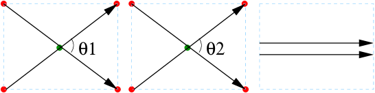
Figure 2: 1/4 BPS cycle. Only the 1/4 cycle $\theta_{1}=\theta_{2}$ can make supersymmetric state and recombine without energy cost. The two cycles are mirror image with respect to the orientifold plane.

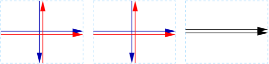
Figure 3: A the branes are on top of orientifold planes: A phase obtained from type I compactification. There is extra gauge symmetry, not visible in gauge thoery, supperted by instantons.

First focus a constant flux configuration, provided by a D-brane background, satisfying the supersymmetry condition (29) and always dualized to a D9-D5 system. All the flux lie in abelian subgroup, thus commute. Among four possible combinations, we take all the sign to be positive for convenience. Plugging it to (30) we have the energy relation [13]

$$\begin{split}H=&\ \tau_{9}V_{2}V_{3}V_{4}\sum_{a=1}^{k}{\rm Tr\,}\big{[}({\bf 1}_{N^{a}}+f_{45,a}^{2})({\bf 1}_{N^{a}}+f_{67,a}^{2})({\bf 1}_{N^{a}}+f_{89,a}^{2})\big{]}^{1/2}\\ =&\ \tau_{9}V_{2}V_{3}V_{4}\sum_{a}{\rm Tr\,}\bigg{[}({\bf 1}_{N^{a}}-f_{45,a}f_{67,a}-f_{67,a}f_{89,a}-f_{89,a}f_{45,a})^{2}\\ &\qquad+(f_{45,a}f_{67,a}f_{89,a}-f_{45,a}-f_{67,a}-f_{89,a})^{2}\bigg{]}^{1/2}\\ =&\ \tau_{9}V_{2}V_{3}V_{4}\sum_{a}\left({\rm Tr\,}{\bf 1}_{N^{a}}-{\rm Tr\,}f_{45,a}f_{67,a}-{\rm Tr\,}f_{67,a}f_{89,a}-{\rm Tr\,}f_{89,a}f_{45,a}\right)\\ =&\ \tau_{9}V_{2}V_{3}V_{4}\sum_{a}N^{a}-\tau_{5}\sum_{a}(V_{4}c_{2,a}^{89}+V_{2}c_{2,a}^{45}+V_{3}c_{2,a}^{67}).\end{split}$$ (31)

Here $k$ is the number of stacks. We stress the negative signs in front of $c_{2}$ are dependent on the sign convention in (29), which will be discussed shortly. We also used the dilation relation (44) and the toron quantization condition (12)

$$\tau_{5} =(4\pi^{2}\alpha^{\prime})^{2}\tau_{9}$$

$$V_{2}V_{3}{\rm Tr\,}F_{45,a}F_{67,a} =V_{2}V_{3}{\rm Tr\,}(F_{45,a})^{2}=N^{a}{m_{1}^{a}m_{2}^{a}\over n_{1}^{a}n_{2}^{a}}=c_{2}^{a}.$$

The DBI energy is expressed in terms of the linear sum of the charges. This is the realization of typical property of BPS saturated states and the relation is exact in $\alpha^{\prime}$ expansion.

Now, this energy is constrained by the RR tadpole cancelation (26).

$$\sum N^{a}=16,\quad\sum c_{2,a}^{ij}=\text{ fixed}$$ (32)

including orientifold mirror images. Definitely the matrix $f_{mn}$ should be embedded $SO(32)$ gauge group. The sum of the rest charges $\sum_{a}c^{ij}_{2,a}$ is dependent on the number of extra O5 planes, which is determined by orbifold. The maximal number of orientifold planes, or disconnected gauge group is therefore four.

We thus have arrived at the important observation: Every consistent system has the same energy because of the tadpole condition. Furthermore, we have supersymmetry, which has many flat directions, thus we expect that many vacua are connected. Among the possibilities, our interest is that from type I compactification, where all the D-branes are on top of orientifold planes.

3.3 Brane recombination

We will seek the possibility that a given intersecting brane setup is continuously connected to a type I compactification. This is done by brane recombination: branes can be deformed yielding to another configuration.

Consider 1/4 BPS cycles first, corresponding to one vanishing angle $\theta_{3}=0$ case as in (11). $T$-dual in 579 directions makes it to D9-branes with magnetic fluxes, which is equivalent to bound D5-branes filling in 89 directions. By a rotation, we can always make the magnetic fluxes into block diagonal and diagonal in the spacetime and the group space, respectively. Therefore, the DBI energy (31) is

$$H=\tau_{9}V_{2}V_{3}V_{4}\sum{\rm Tr\,}({\bf 1}_{N^{a}}+f^{2}_{45,a})=\tau_{9}V_{2}V_{3}V_{4}\sum N^{a}+\tau_{5}V_{2}\sum c_{2,a}$$ (33)

The sign of the second term is always positive for any choice of the sign.

From worldsheet bosonic spectrum, we have two light complex scalars with masses

$$M_{1}^{2}={1\over 2\pi\alpha^{\prime}}(\theta_{1}^{a}-\theta_{2}^{a})=-M_{2}^{2}$$ (34)

where $\theta_{i}^{a}$ is the angle of 2-cycles $\pi_{a}$ in $i$th $T^{2}$. We have a tachyon for generic angles $\theta_{1}^{a}\neq\theta_{2}^{a}$, which reflects the instability of vacuum, arising from wrong expansion of the (string) field theory. This tachyon condenses and rolls down to a true runaway vacuum [62]. However, if

$$\theta_{1}^{a}=\theta_{2}^{a}\quad\text{ for all }a,$$ (35)

there is no tachyon. This demonstrates that we have supersymmetry, since the superpartner fermions are always massless. This condition is translated into the condition on magnetic field

$$F_{45}^{a}=\pm F_{67}^{a}\Leftrightarrow*_{4}F_{mn}^{a}=\pm F_{mn}^{a}.$$ (36)

Although we have made use of factorizable cycle, the latter (anti-)self-dual condition is general for nonfactorizable cycle [63] $m,n=4,5,6,7$. The Hodge-dual operator is in the 4567-direction. Then the preserved supersymmetry component $\epsilon$

$$\delta\chi=\Gamma^{\mu\nu}F_{\mu\nu}\epsilon=(\Gamma^{45}\pm\Gamma^{67})F_{45}\epsilon=0$$ (37)

is same for every intermediate step. Since supersymmetry is preserved, there is no cost on “marginal” deformation. Therefore we see, for 1/4-cycle, there is a recombination [6]

$$\begin{split}&(n_{1},m_{1})(n_{2},m_{2})(1,0)+(n_{1},-m_{1})(n_{2},-n_{2})(1,0)\\ &\to 2n_{1}n_{2}(1,0)(1,0)(1,0)+2m_{1}m_{2}(0,1)(0,1)(1,0).\end{split}$$

which preserves the energy and charge. The two phases are drawn in Figs. 2 and 3. (The parallel phase cannot be described by gauge theory, because of the vertically running brane.)

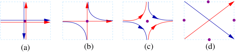
Figure 4: Intermediate steps, governed by the supersymmetry condition (29), which is a generalization of self-dual condition. The points denote intersections, some of which are identified. During the recombination the RR charges and the (sum of) volumes are conserved. Only one two-torus is drawn.

The recombination of 1/4 cycles is well known as fattening and shrinking instanton. We take a simplified example of bound state of two D5 and two D9 branes in a rectangular $T^{4}$ in 6789 direction. When we make a $T$-dual in 68-direction, the D5 and D9 branes become two D6 brane at right angles, as in Fig. 3. Definitely the degree of freedom is $U(2)\times U(2)$. The gauge theory cannot describe this, because in the original picture, there is an extra, singular $U(2)$ gauge symmetry supported by instanton [54]. A string between D5 and D9 brane transforms as bifundamental $\bf(2,2)$ denoted $h_{M}^{Am}$ in ref. [55]: $m$ and $M$ are internal index of D5 and D9 gauge theory, respectively, and $A$ is R-symmetry index $SU(2)_{R}$ as a part of $SO(4)$ internal Lorentz symmetry transverse to D0-brane. $h^{A}$ corresponds to a Higgs field, with the charge parameterized by $m$ and $M$, and describes the scale size of the instanton. Among them, there is a setup in which we have two tilted intersecting brane, depicted in Fig. 2. We see the resulting two brane has separated by the diagonal distance of the torus, as in Fig. 4 (b) or (c). The intersection point is specified by D0-D0 state denoted as $X^{AY}$ in [55], where $Y$ is leftover $SU(2)$ index of above transverse $SO(4)$. We can generalize this to any of D5-D9 bound state.

Although the above phenomena is not realized by gauge theory, a further Higgsing can be [8]. A bifundamental representation, corresponding to off-diagonal elements in (16), further breaks the “visible” gauge symmetry and reduces the rank. The electroweak Higgs mechanism is a good example. Note that, for the intersecting setup, turning on the constant VEV does not affect F-term condition (29) given by derivatives. However to fulfill D-term condition, the $i$th block of the coordinate matrix $X^{m}_{a}$ should be either diagonal or proportional to others. The former condition is responsible for parallel translation discussed in introduction. The latter completely determines the form of $X^{m}_{a}$ if the one component is determined. In this sense the supersymmetric deformation is encoded in one dimensional degrees of freedom $b^{1}(\pi)$. For example, we have parameterized the 1/4 cycles (11) as (12) and it is the slope of tilted branes, as in (3),

$$\frac{1}{2\pi\alpha^{\prime}}X^{2}_{a}={2\pi\over A}{m^{a}_{1}\over n^{a}_{1}}{\bf 1}_{N^{a}}X^{1}+A^{0}_{2,a}$$ (38)

Due to off-diagonal elements, we lost the geometrical interpretation. Being Hermitian, we seems to be able to recover the geometry if we diagonalize all the $X^{m}$ simultaneously, this would not be compatible with the torus embedding. Anyway, in the noncompact limit, or the local limit around the intersections, diagonalization gives curves in general, also look like Fig. 4. Also in $T$-dual space, the magnetic flux is not uniform which is possible because both the instanton field and the energy scale the same. In the limit of (at least one) off-diagonal components of $X^{2}$ goes to large, the finite $X^{2}$ dependence goes to zero, leaving the parallel branes. This is again the same kind of Higgs mechanism, and the states corresponding to off-diagonal element transform as ifundamental representation. Of course, every intermediate curves has the same volume since the constant Wilson line is only responsible for translation; In the $T$-dual picture the DBI action gives the volume itself, as a function of derivatives. We can relate this Higgs mechanism with D-term supersymmetry breaking.

Describing tilted or intersecting brane does not require any further moduli [1]. It is determined by internal geometry, here torus with two complex moduli, and quantization condition (6). Therefore the recombination is the only possible way to change intersecting setup involving chirality: There can be a local change in chirality [10], as clearly seen in Fig. 4, and the intersection number (18), but the gross chirality does not change since the RR charges is invariant at every step. We can see this from the fact that Chern numbers are not changed thus does not affect total anomaly polynomial, reflecting again the fact that the anomaly is controlled by RR charges.

We have some other descriptions. The conditions (35) and (37) are local relations [65]. It is nothing but the holomorphic Cauchy–Riemann condition

$${\partial x^{5}\over\partial x^{4}}={\partial x^{7}\over\partial x^{4}},\quad{\partial x^{5}\over\partial x^{6}}=-{\partial x^{7}\over\partial x^{6}}.$$ (39)

We parameterize the curve as $x^{5}+ix^{7}$ as a function of $x^{4}+ix^{6}$. The first is equivalent to Eq. (35), follows from $\tan(\theta_{1}-\theta_{2})\propto\tan\theta_{1}-\tan\theta_{2}=0$. Also if we require the rotation to be unitary, we obtain the latter. The complexified function $x^{5}+ix^{7}$ is analytic and this fact guarantees the holomorphicity in entire domain. It is well known that complex curve in two complex dimension always span the minimal volume [57], agreeing with (31). To the other way around, since in two dimension, a holomorphic transformation is conformal transformation, it always preserves relative angles (35) at every point. Such property of minimality is known as calibration between two cycles, and the corresponding (relative) cycle is called special Lagrangian (SL) cycle [57]. In ref. [32, 10] an algebraic description of such interpolating curve is presented. Similarly we have the anti-holomorphic condition from anti-self duality.

We saw that supersymmetry-preserving deformation is parameterized by Wilson lines of one coordinate $X^{m}$, and this provides the special case of McLean’s theorem, applicable to the former case also [46]: For a compact SL cycle $\pi$ in an (almost) Calabi–Yau manifold, the moduli space of deformation of $\pi$ is a smooth manifold of dimension $b^{1}(\pi)$, where $b^{1}(\pi)$ is the first Betti number of $N$.

The above D0-D4 bound state is $U$-dual to (F,D$p$) bound state which is interpreted as the electric flux on D-branes [7, 12]. The above BPS equation becomes string “junction condition” [26] (In the self-dual case $g=1$.) and we can clearly see the supersymmetry condition at every local point, with the same supersymmetry components preserved. In this picture we can also see the no-energy-cost property under marginal deformation and the specific shape of final state [12]. The DBI energy is $V\sqrt{-\det{(1+2\pi\alpha^{\prime}F)_{\mu}}^{\nu}}.$ When we have purely magnetic flux, this is nothing but the winding volume of torus $V\sqrt{1+(2\pi\alpha^{\prime}F)^{2}}=V\sqrt{1+\tan^{2}\theta}=V_{\rm cycle}$, agreeing with intersecting brane case. But when we have contribution from fundamental string, which carries NS-NS flux, which is equivalent to electric field component. The size of electric and magnetic fluxes should be equal due to BPS condition, so the determinant becomes 1, which shows independence of cycle. Although there are not always one to one correspondence among dual theories, at least it exhibit the property that there is no volume dependence.

The case of 1/8-cycles is less trivial. From the dependence on $N,c_{2}^{ij}$, we see that the system is $T$-dual to D9-$\overline{\rm D}$5-$\overline{\rm D}$5-$\overline{\rm D}$5 bound state. Three $\overline{\rm D}$5-branes span along 89,45, and 67, directions. Protected by supersymmetry, the bound state energy is again marginal. Not like the 1/4 BPS cycle case, here the energy is dependent on the choice of the signs in (29), but the physics is the same. The system at hand seems like $T$-dual to D3-D9 bound state, since one D6 becomes pointlike in six compact dimension while the other becomes D9, however it is not. A D3 charge would appear as a single $c_{3}$ and D3-D9 system has only one sector having positive zero point energy thus cannot be bound state. The D9-$\overline{\rm D}$5-$\overline{\rm D}$5-$\overline{\rm D}$5 bound state has four disconnected sector, only one of which has lowest mass zero and other three lowest masses are positive. This is the consequence of the supersymmetry condition (29). Note also we can flip some of the antibranes into D-branes, which amounts to flipping some of the signs of the fluxes $f_{mn}\to-f_{mn}$. However we can veryfy that not all of them can be. This property shows the reason why this system cannot be reduced into D9-D5 systems. Being quadratic, the leading order kinetic terms are invariant.

Still, there is a recombination, since for generic angles the system has a tachyon, which again signals the recombination, and the supersymmetric condition become the one of marginal stability. As in the 1/4 case, VEVs of all the $\overline{\rm D}$$5_{i}$-D9 Higgs is will describe recombination, however, now the condition (29) relates all of them and thus is more strict. At the moment there is no concrete solution to 1/8 case, from a general intersection to the trivial one where every D-branes are on top of orientifold plane. However by energetics and charge conservation, this is highly likely. Finding the generalized instanton solution for 1/4 cycle [13] would be interesting investigation.

4 Gauge coupling unification

We saw that each simple or Abelian subgroup came from the breaking of a single unified group. Thus it might be surprising if each the subgroup has a different gauge coupling. However we will see that, because of the nonlocal property of DBI action, the background flux can give rise to different factor for each subgroup, leading to a different four dimensional gauge coupling.

4.1 Gauge coupling

Expanding to the quadratic order in $\alpha^{\prime}F_{\mu\nu}$, the DBI action (30) reduces to ($p$+1)-dimensional Yang–Mills (YM) action,

$$S_{p}=-{T_{p}(2\pi\alpha^{\prime})^{2}\over 4g}\int d^{p+1}x~{}{\rm Tr\,}F_{\mu\nu}F^{\mu\nu}$$ (40)

where $g=e^{\langle\Phi\rangle}$ is the string coupling. We are using the trace in the fundamental representation of $U(N)$. Therefore, the YM coupling is

$$g^{2}_{p+1,\rm YM}=(2\pi)^{p-2}g\alpha^{\prime(p-3)/2}.$$ (41)

For the action to be invariant under $T$-duality, the dilaton should transform under $T$-duality. Recover the dilation dependence and consider a compactification in $p$-direction with the circumference $L_{p}$. Compare the mass of D$p$-branes and its $T$-dual D$(p-1)$-brane, which are the same,

$$T_{p}e^{-\Phi}L_{p}=T_{p-1}e^{-\Phi^{\prime}}.$$ (42)

For them to be the same, the dilatons should behave as

$$e^{\Phi^{\prime}}={\alpha^{\prime 1/2}\over L_{p}}e^{\Phi}.$$ (43)

Hence the gravitational coupling and gauge coupling, which are proportional to $e^{-\Phi}$ It will be convenient later to define

$$\tau_{p}\equiv T_{p}e^{-\Phi}=\tau_{p-1}L_{p}^{-1},$$ (44)

since $\tau$ times the volume occupied by D-brane is an invariant of $T$-duality. This is nicely expressed as the relation between gravitational and gauge coupling

$${g_{\rm YM}^{2}\over\kappa}=2(2\pi)^{7/2}\alpha^{\prime}$$ (45)

where the factor 2 with a single orientifold plane, for any number of compact extra dimensions. When all the branes are on top of orientifold plane, this is the same relation to that of type I string.

The tilted D-brane is represented by a constant magnetic flux. Now we calculate the actual fluctuation around D-brane background [15, 16]

$$A_{\mu}=A_{\mu}^{0}+\delta A_{\mu}.$$ (46)

In fact the expansion is more involved, since fluctuations do not commute with background $[A_{\mu}^{0},\delta A_{\mu}]\neq 0.$ For nonabelian DBI action, the trace in (30) should be done on the group space. Because the noncommutivity, how to evaluate the trace is not known so far. Replacing trace with symmetrized trace [33] ${\rm Tr\,}\to{\rm STr\,}$ works very well. This is known not fully consistent remedy, since at the quadratic order, spectrum of intersecting brane does not match with the string calculation [35, 15].

Plugging (46) into the DBI action (30) and expanding up to the quadratic order in $\tilde{F}_{\mu\nu}\equiv 2\partial_{[\mu}\delta A_{\nu]}-i[A_{\mu},\delta A_{\nu}]$, around

$${({\bf 1}+f){{}_{\mu}}^{\nu}}.$$ (47)

The raising and lowering indices are done with the ‘genuine’ flat metric $\eta_{\mu\nu}$. Here we keep in mind that this has both the Lorentz and the gauge group index, and we suppressed the latter. We can decompose its inverse to a symmetric and antisymmetric part in Lorentz index,

$$({\bf 1}+f)^{-1}=({\bf 1}-f^{2})^{-1}-f({\bf 1}-f^{2})^{-1}\equiv g+b,$$ (48)

where the inverse is done on both the Lorentz and the gauge group space. The DBI action becomes

$${\rm STr\,}\sqrt{\det({\bf 1}+f)}\sqrt{-\det({\bf 1}+g\tilde{F}+b\tilde{F})}$$ (49)

4.2 Fluctuation spectrum

We expand the action (49) to the quadratic order in fluctuation $O(\alpha^{\prime}\tilde{F})^{2}$. The leading order constant term is the background contribution (33)

$$S=-\tau_{9}\int d^{10}x{\rm Tr\,}{\bf 1}_{32}-{1\over 4g_{\rm YM}^{2}}\int d^{10}x{\rm Tr\,}F_{MN}^{2}+\cdots.$$ (50)

The gauge group for the first term is always $SO(32)$ with type I coupling $g_{\rm YM}$ (45), since this is the expectation value of a constant magnetic flux in type I string theory. If we have more orientifold plane(s), there can be other nonzero second Chern numbers, thus be as many $SO(32)$, denoted by ellipsis. However all the couplings are the same, since the orientifold planes and the D-branes on top of them are exchangeable by a $T$-duality (which is not visible in gauge theory).

Now consider the fluctuation around the above background—of the 1/4 cycle first. We have

$$L={\rm STr\,}({\bf 1}+f_{45}^{2})\left(g_{\mu\nu}\tilde{F}^{\nu\lambda}g_{\lambda\sigma}\tilde{F}^{\sigma\mu}+b_{\mu\nu}\tilde{F}^{\nu\lambda}b_{\lambda\sigma}\tilde{F}^{\sigma\mu}\right)+\text{(topological terms)}.$$ (51)

The total derivative term becomes topological term and contributes to the zero point energy, agreeing with the worldsheet calculation [16]. The nonvanishing contribution of $({\bf 1}+f)^{-1}$ is only the symmetric part $g$ [15] having eigenvalues

$$g_{mn}=\begin{pmatrix}(1+f_{45}^{2})^{-1}{\bf 1}_{2}&&\\ &(1+f_{67}^{2})^{-1}{\bf 1}_{2}&\\ &&{\bf 1}_{2}\end{pmatrix},\quad g_{\mu\nu}=\eta_{\mu\nu}.$$ (52)

Thus we have the action

$$\begin{split}2\tau_{9}&(2\pi\alpha^{\prime})^{2}\int d^{10}x{\rm STr\,}({\bf 1}+f_{45}^{2})g^{MN}\tilde{F}_{NP}g^{PS}\tilde{F}_{SM}\\ &=S_{\rm 6D}-\frac{1}{4g_{\rm YM}^{2}}\int d^{10}x{\rm STr\,}({\bf 1}+f_{45}^{2})\tilde{F}_{\mu\nu}\tilde{F}_{\mu\nu}+\dots\end{split}$$ (53)

The D9 and D5 fluctuation is forced to be identified, which is exactly the prefactor affecting the canonical normalization. For 012389 direction, the prefactor persists, however for 4567, which is the brane-tilted space, the prefactor exactly cancel out the metric.

In the low energy limit where extra fluctuation is negligible $\tilde{F}_{mn}\simeq 0$, we have four dimensional effective YM theory

$$S=-\frac{v_{6}}{4g_{\rm YM}^{2}}\int d^{4}x{\rm Tr\,}({\bf 1}+f_{45}^{2})\tilde{F}_{\mu\nu}\tilde{F}_{\mu\nu}+\dots.$$

with

$${\bf 1}+f_{45}^{2}=\begin{pmatrix}(1+(\frac{m^{1}}{n^{1}})^{2}){\bf 1}_{N^{1}}&&&\\ &(1+(\frac{m^{2}}{n^{2}})^{2}){\bf 1}_{N^{2}}&&\\ &&\ddots&\\ &&&(1+(\frac{m^{k}}{n^{k}})^{2}){\bf 1}_{N^{k}}\end{pmatrix}.$$ (54)

Note that, the $a$th gauge field come from the $a$th block of rank $N^{a}$. The effective gauge coupling constant is

$$g_{4,i}^{2}=g_{\rm YM}^{2}/V_{{\rm cycle},i}$$ (55)

from the canonical normalization. This is so because the gauge field background described by DBI action multiplies the kinetic terms. Since it has nontrivial nonabelian structure, it gives different couplings to each subgroup. Being described by DBI action, a single unified group $G$ can give different gauge couplings for each unbroken factor groups $H_{i}$. Without introducing extra volume moduli, nor introducing nonabelian structure to it, we can have different gauge couplings for different gauge groups originating from the same $SO(32)$.

Near and above the string scale $M_{s}\sim\alpha^{\prime-1/2}$, the size of fluctuation becomes comparable to that of the background $\delta A\sim A_{0}$, therefore the above expansion breaks down. Above this scale also the extra dimensions open up, thus the theory is ten dimensional type I string theory or at least its supergravity approximation. This is the reason why the YM dynamics cannot catch such dependence. However we can understand, at least, how spontaneous symmetry breaking could lead a different coupling for each gauge group at the breaking scale. This is explained by brane recombination. Vacua with different four dimensional couplings are connected by energy costless deformation, which is possible since four dimensional coupling is controlled by dynamics of extra dimension.

In the internal dimension, the canonical normalization is not affected, thus the gauge coupling is the same. However in the potential term, there is a rescaling by one factor of $g$ [15]. We have used

$${(1+f)_{\mu}}^{\rho}{g_{\rho}}^{\nu}={\bf 1}+\text{ (antisymmetric tensor)},$$

for the 45 and 67 components, where the latter does not contribute in the Lagrangian, and the YM coupling relation.

$$S_{\rm 6D}=-\frac{1}{4g_{\rm YM}^{2}}\int d^{10}x{\rm STr\,}\tilde{F}_{0m}\tilde{F}_{0m}-\frac{1}{4g_{\rm YM}^{2}}\int d^{10}x{\rm STr\,}\tilde{F}_{ik}g^{kl}\tilde{F}_{li}\\$$

The factor 2 comes from D9 and D5 contributions, and the resulting two YM actions correlated. For self-dual case, this action reproduces completely the same spectrum as worldsheet analysis with the symmetrized trace prescription

$$-\frac{1}{f_{45}}\int_{0}^{-f_{45}}df^{\prime}g_{45}=-\frac{1}{f_{45}}\int df^{\prime}(1+f_{45}^{\prime 2})^{-1}={\theta_{1}\over\tan\theta_{1}}$$ (56)

and the metric dependence modifying momentum-winding quantum numbers. The only difference is that we do not have overall factor in (51). This prescription correctly reproduces the spectrum, as obtained from the worldsheet theory [16, 15].

Let us come to the 1/8 BPS cycles with no zero eigenvalues for $\theta_{i}$. In this case, there is no known prescription to produce the correct spectrum. We examine the reason here. The leading zeroth order contribution (31), which looks like instanton density, must be still the usual gauge kinetic term with background value. Again, supersymmetry condition (29) plays a similar role as self-dual condition

$$\begin{split}&f_{45}f_{67}+f_{67}f_{89}+f_{89}f_{45}\\ &=\frac{1}{2}(-f_{45}^{2}-f_{67}^{2}-f_{89}^{2}+(f_{45}+f_{67}+f_{89})^{2})\\ &=-\frac{1}{4}f_{mn}^{2}+\frac{1}{2}(f_{45}f_{67}f_{89})^{2}.\end{split}$$ (57)

Note that we have recovered the correct sign for the kinetic term. Therefore we have Hamiltonian density

$$\frac{1}{4g^{2}_{\rm YM}}\int d^{10}x({\rm Tr\,}{\bf 1}+{\rm Tr\,}F_{MN}^{2}+{O}(\alpha^{\prime}F)^{4}).$$ (58)

Its fluctuation is expected to be give the desired gauge theory. However there have no expansion of DBI action to the desired YM action. We claim that the reason can be again tracked by nonlocality of stringy physics at scale $\alpha^{\prime-1/2}$.

Figure 5: Interbrane interaction is nonlocal, thus we look at the theory in the vicinity of a specific $\overline{\rm D}$5 brane. Two $\overline{\rm D}$5-branes are shown.

In the vicinity of 45 brane, we can see the effect of $\overline{\rm D}$5-brane along 45 direction, as gauge theory again. However we cannot see the rest of gauge theory here, because of nonlocality: They are cast as the higher order terms, because of the string stretched between other $\overline{\rm D}$5-branes along 67 and 89 directions. They are suppressed by $(2\pi\alpha^{\prime})^{2}$, which, by dimensional analysis, shows that the interaction requires four more dimensions. Fig. 5 shows that there are no intersection in this $\overline{\rm D}$5-D9 picture and the interaction is nonlocal, which is the higher terms of DBI action. In $T$-dual picture, in this 1/8 BPS case, the magnetic flux due to D5 brane is not completely spread over the transverse four dimension inside D9, therefore there is no interaction among fluxes of different $\overline{\rm D}$5 branes. However there is a local relation with space-filling D9-branes with this $\overline{\rm D}$5-brane, being the rank $N$ gauge group. The permutation symmetry of the terms, which is again the $T$-dual relation, shows that we have similar effects around other $\overline{\rm D}$5-branes.

What would be the non-supersymmetric coupling relation? We realize that, the above supersymmetry relation is nothing but the BPS inequality. For non-supersymmetric system, still the above action (31) is the leading order terms, and the non-supersymmetric term will be added to the higher orders from ${O}(\alpha^{\prime}F_{\mu\nu})^{4}$. Admittedly the BPS condition (29) make the supersymmetric expansion (31) exact. Also note that this relation holds for non-factorizable torus and orientifold. Although in the nonsupersymmetric case it is not clear that we have a similar condition to self-duality, we know that D-brane plays the double role as instanton and gauge theory even in nonsupersymmetric case. So it is reasonable to convert the Chern–Simon $F^{2}$ terms to gauge kinetic ones and expect higher order terms as non-local interactions.

We have briefly commented on a winding state by $w$ times, or bound state of $w$ branes. From the former picture, it is evident that the winding volume is $w$ times larger than the single one. However DBI action cannot reproduce it, and in fact we have no tool taking into account it.

4.3 Weak mixing angle

The conventional Grand Unification based on groups such as $SU(5)$ and $SO(10)$ naturally give rise to nontrivial weak mixing angle

$$\sin^{2}\theta_{W}\equiv{g_{L}^{2}\over g_{\rm em}^{2}}=\frac{3}{8}$$ (59)

at the unification scale. Within the current experimental limit, this is the most desirable value. It is purely given by group theory provided that there is a single gauge coupling. This is also naturally realized in the heterotic string compactification [61], although $U(1)$ factor is determined by model basis.

In the intersecting brane scenario, the natural gauge group is not a simple but a semisimple group containing $U(1)$. For example the $U(1)$ factor inside $U(N)$ is identified as the trace, and the canonical normalization gives

$$A_{\mu,U(1)}=\frac{1}{N}{\rm Tr\,}A_{\mu,U(N)},\quad g^{2}_{U(1)}=\frac{2}{N}g^{2}_{U(N)},$$ (60)

for normalization ${\rm Tr\,}T^{a}T^{b}=\frac{1}{2}\delta^{ab}$ for fundamental representation of $U(N)$. The hypercharge is given by the linear combination of several $U(1)$s, $Q_{Y}=\sum_{i}C_{i}Q_{i}$. According to term, canonical normalization of gauge kinetic term yields,

$$\frac{1}{g^{2}_{Y}}=\sum_{i}{N_{i}C_{i}^{2}\over 2}\frac{1}{g^{2}_{i}}.$$ (61)

For the charge assignment (20), we have

$$\frac{1}{g^{2}_{Y}}=\frac{1}{6}\frac{1}{g^{2}_{C}}+\frac{1}{g^{2}_{L}}+\frac{1}{2}\frac{1}{g^{2}_{R}}=\frac{5}{3}\frac{1}{g^{2}},$$ (62)

in the unified coupling limit $g=g_{L}=g_{R}=g_{C}$. We have the desired relation

$$\sin^{2}\theta_{W}={1\over g_{Y}^{2}/g^{2}+1}=\frac{3}{8}$$ (63)

at the unification scale.

The reason for the correct value can be tracked to charge embedability into $SO(10)$. We note that in the Madrid model discussed above, the three anomalous extra $U(1)$ factors can be interpreted as baryon $Q_{B}$ and lepton $Q_{L}$ and Peccei–Quinn numbers $Q_{R}$

$$A_{\mu,B}=\frac{1}{3}{\rm Tr\,}A_{\mu,U(3)_{C}},\quad A_{\mu,L}=\frac{1}{2}{\rm Tr\,}A_{\mu,U(2)_{L}}.$$ (64)

These are broken by generalized GS mechanism, and become global symmetries below the breaking scale. This provides a good explanation of the accidental symmetries of the baryon and the lepton numbers in the Standard Model, which remains continuous. Higgsing with charged field always leaves the discrete subset of the symmetry. The relation (62) comes from the hypercharge relation in $U(1)_{B-L}\times U(1)_{R}\subset SO(10)$

$$Q_{Y}=Q_{B}-Q_{L}-Q_{R}=\frac{1}{3}Q_{C}-Q_{L}-Q_{R},$$ (65)

reproducing (63). Obviously, matter spectra do not fit to the spinorial ${\bf 16}$. However $SO(32)$ is the group that can embrace all of these features. Note that, if we obtained $SU(2)_{L}=Sp(1)$, rather than one above $SU(2)_{L}\subset U(2)_{L}$, we could not reproduce the desired coefficient $1$ in the second term on the (62), since $U(1)_{L}$ then would be an independent Abelian gauge group having normalization $1/2$. Since the baryon and the lepton numbers are conserved, there is no fast proton decay and the neutrino is only Dirac.

Therefore in the intersecting brane scenario, the running of gauge couplings from electroweak scale would not be changed provided the coupling is unified. For one option, if two of the gauge group is related by some symmetry such as parallel separation or reflection due to orientifold, their couplings are exactly the same [4, 6]. The other possibility is that the discrepancy might be approximately compensated by loop threshold corrections [36]. As bottom-up approach, the possible values scenarios for the desired weak mixing angle is analyzed in [37].

5 Type I compactification

The modern viewpoint of type I string is type IIB string with one O9-plane and 16 D9-branes [50]. Introducing a D-brane requires an orientifold plane with the same dimensionality for the consistency. By $T$-duality, we can always convert these D-branes and orientifold to 9+1 dimensional ones. Also, we have seen that by recombination, we could make all the D-branes coincident on the orientifold planes. Therefore we naturally expect that all the intersecting brane models should be to type I theory compactified on orbifold or its $T$-dual, which we will argue here.

The symmetry possessed by an open string is broken by projections associated with elements in orientifold group $P_{1}\cup\Omega P_{2}$ [38, 39, 28]. We only consider a case having a geometric meaning $P_{1}=P_{2}=P$. The action of an element $g\in P$ and $\Omega h\in\Omega P$ act on Chan–Paton factor as

$$\begin{split}g&:|\psi,ij\rangle\to(\gamma_{g,p})_{ii^{\prime}}|g\psi,i^{\prime}j^{\prime}\rangle(\gamma_{g,q})^{-1}_{j^{\prime}j}\\ \Omega h&:|\psi,ij\rangle\to(\gamma_{\Omega h,p})_{ii^{\prime}}|h\psi,j^{\prime}i^{\prime}\rangle(\gamma_{\Omega h,q})^{-1}_{j^{\prime}j}\end{split}$$ (66)

where the second subscripts $p,q$ denote the dimensionality of branes. We defined $\gamma_{\Omega h,p}\equiv\gamma_{h,p}\gamma_{\Omega,p}$ since $\Omega h=\Omega\cdot h$ and $\gamma_{k,p}=\gamma_{1,p}^{k}$ thus we have $\gamma_{1,p}^{N}=\pm 1$. The surviving fields are invariant ones under the projection (66).

The orbifold group $P$, compatible with the lattice translations defining the torus, should be a discrete subgroup of $SU(3)$ holonomy, to preserve at least $N=1$ supersymmetry in four dimension [59, 41]. An orientifold projection breaks half of the supersymmetry. In the closed string sector, such a choice guarantee at least one of the spinorial component of RNS or NSR state invariant under holonomy. In the open string sector, this orbifold images are connected again by the holonomy, so there is a compatible $N=1$ supersymmetry. Such crystals are classified and finite in numbers [60, 41].

Essentially, type II string theory with a O-plane is ($T$-dual to) type I string theory. We saw that there is at least one such orientifold plane required. This can always be converted to O9 plane by $T$-duality. In general, orientifold group is generated by orbifold actions $g\in P$ and worldsheet parity reversals

$$\Omega\prod R_{m}(-1)^{F_{L}},$$

where $R_{m}$ are spatial reflections of compact $x^{m}$ directions and $F_{L}$ is the spacetime fermion number. This O$p$ plane is lying (or, defined) on the fixed plane under $\prod R_{m}(-1)^{F_{L}}$. By the $T$-dual $\prod R_{m}(-1)^{F_{L}}$, we can always convert it to $\Omega$, while orbifold group $P$ is untouched. The type IIB theory with orientifold element $\Omega$ is type I theory, so that every theory containing orientifold is regarded as compactification of type I string theory with $P$. It follows that the orbifold group $P$ completely determines additional orientifolds and thus gauge group. (We will consider an asymmetric orbifold $\hat{P}$ shortly.)

Whenever we have a D-brane it is always $T$-dual to D9-brane, so there is divergence proportional to the ten dimensional volume factor $v_{4}v_{6}$ [38]. It is canceled by introducing O9 plane

$${v_{4}v_{6}\over 16}\left\{32^{2}-64{\rm Tr\,}(\gamma_{\Omega,9}^{-1}\gamma_{\Omega,9}^{\top})+({\rm Tr\,}(\gamma_{1,9}))^{2}\right\}$$ (67)

and 32 D9-branes and imposing

$$\gamma_{\Omega,9}^{\top}=+\gamma_{\Omega,9}.$$ (68)

In the standard compactification on symmetric orbifold $P$, in addition to this O9, there can be other orientifold planes when the orbifold group is compatible with ${\bf Z}_{2}$. Consider the $P={\bf Z}_{N}$ orbifold first. For $N$ odd, the remaining divergence is proportional to $V_{4}$ which is the regularized noncompact dimensional volume. It should be finite otherwise we have no physics to regulate in that direction. In this case, with a single orientifold plane, it is shown [40] that there is no nontrivial supersymmetric setup, except one where all the D-branes are on top of orientifold plane. The constraint comes from the tadpole cancelation condition of both RR and NSNS charges. Before constraining tadpole condition, we have potentials for complex structure moduli and dilaton. From the cancelation condition of both, there arises an inequality which is only saturated only when the complex structure makes all the D-branes on top of O-plane.

For $N$ even, the remaining divergence is proportional

$${v_{6}\over 16v_{4}}\left\{32^{2}-64{\rm Tr\,}(\gamma_{\Omega R,5}^{-1}\gamma_{\Omega R,5}^{\top})+({\rm Tr\,}(\gamma_{1,5}))^{2}\right\}$$ (69)

to $1/v_{4}$, which manifestly shows that it is $T_{5678}$-dual to the above divergence term, since it relates $v_{4}\leftrightarrow 1/v_{4},\gamma_{\Omega,9}\leftrightarrow\gamma_{\Omega R,5}$. This means, introducing 16 D5-branes in these direction cancels the divergence, and the requiring replacement $\gamma_{\Omega R,5}^{\top}=+\gamma_{\Omega R,5}$ shows again the $T$-duality. $N$ even has order 2 section and this harbors exactly such the O5 and D5 planes. It follows

$$\gamma_{1,9}^{N}=-1,\quad\gamma_{1,5}^{N}=-1$$ (70)

There is an extra piece from the cylinder amplitude proportional to $v_{6}$ only, which seems not has such $T$-duality, but it vanishes for an appropriate choice of $\gamma$ basis. However other divergences arising from ${\bf Z}_{4},{\bf Z}_{8},{\bf Z}_{8}^{\prime}$ and ${\bf Z}_{12}^{\prime}$ orbifolds, proportional to $v_{6}/v_{4}$ cannot be canceled. So these choices of orbifolds are not consistent for the symmetric orbifold compactification. We will see, however, these orbifolds can be consistent when we consider asymmetric orbifolds.

For $P={\bf Z}_{M}\times{\bf Z}_{N}$ orbifold, extra orientifold planes can emerge depending on whether such ${\bf Z}_{M}$ or ${\bf Z}_{N}$ contains order two element. We will see that we can have either one or four orientifold planes in total, if we take into account supersymmetry. The latter case is both $M,N$ even and contains the following ${\bf Z}_{2}\times{\bf Z}_{2}$ orbifold group as a subgroup. It is generated by $\{\theta_{1},\theta_{2}\}$ where

$$\begin{split}\theta_{1}:(z_{1},z_{2},z_{3})\leftrightarrow(-z_{1},-z_{2},z_{3}),\quad\theta_{2}:(z_{1},z_{2},z_{3})\leftrightarrow(z_{1},-z_{2},-z_{3}).\end{split}$$ (71)

Thus we have a nontrivial order 2 element $\theta_{1}\theta_{2}:(z_{1},z_{2},z_{3})\leftrightarrow(-z_{1},z_{2},-z_{3})$. Each of them has a 5+1 dimensional fixed planes thus can harbor O5 plane. Still in this case, now the $5$-lanes are labeled as $5_{i}$, each divergence condition is exactly the same as (69) for each $i$th orientifold direction [58].

From these conditions, we can cancel the diagram and this give rise to conditions on the projection matrices $\gamma$, and applying these to (66) we have broken gauge group. They are determined without ambiguity. Note that this will be given as branching rules. For example the compactification on the orbifold $T^{6}/({\bf Z}_{2}\times{\bf Z}_{2})$ [58]. And they are explained. There exists a discrete torsion which produces a different form of one loop amplitude [49], we will not consider it here.

It follows that the $Sp(k)$ groups can only appear as broken $SO(32)$, which takes into account small instantons [54].

For consideration of $T$-duality one should be careful to mention $P$. It was noted in [51] that $T$-duality flips sign asymmetrically to the left and the right mover,

$$X_{L}=X^{\prime}_{L},\quad X_{R}=-X^{\prime}_{R}$$ (72)

if we do $T$-dual odd times to a two-torus parameterized by

$$(z_{L},z_{R})\leftrightarrow(\bar{z}_{L}^{\prime},z_{R}^{\prime}),$$ (73)

which is as good as complex conjugation in $T$-dual space. Then the orbifold action

$$g:(z_{L},z_{R})\to(e^{i\theta}z_{L},e^{i\theta}z_{R})$$ (74)

becomes asymmetric in $T$-dual direction

$$\hat{g}=TgT^{-1}:(z_{L}^{\prime},z_{R}^{\prime})\to(e^{-i\theta}z_{L}^{\prime},e^{i\theta}z_{R}^{\prime})$$ (75)

The cases of ${\bf Z}_{2}$ and ${\bf Z}_{2}\times{\bf Z}_{2}$ are exceptions, since $e^{\pi i}$ is just a change of sign, so asymmetric orbifold is the same as symmetric orbifold.

The orientifold group is $\Omega P$, which changes into $\Omega RP$ by $T$-duality in $R$ direction, whereas the orbifold group remains as $P$. Consider $T$-duality in $579$ direction, which is conveniently realized as

$$R:(z_{1},z_{2},z_{3})\leftrightarrow(\bar{z}_{1},\bar{z}_{2},\bar{z}_{3}).$$ (76)

Now the orientifold group is $\Omega RP$, whereas the orbifold group $P$ remains invariant. It is easily checked that all the O9 and O5 planes becomes O6 planes,

$$\Omega,\Omega\theta_{1},\Omega\theta_{2},\Omega\theta_{1}\theta_{2}\leftrightarrow\Omega R,\Omega R\theta_{1},\Omega R\theta_{2},\Omega R\theta_{1}\theta_{2}$$ (77)

not intersecting among themselves. Since this is the most nontrivial setup, this proves that every D$p$ and O$p$ planes can be mapped to D6/O6 planes, which are desirable in the $M$-theory dual picture. These planes are (24). It is stressed that both pictures are equivalent.

For supersymmetric system, we cannot have D-branes other than the O9/D9 and/or O5/D5 considered above. By $T$-duality, fixing one orientifold as O9, let us then count the lower dimensional orientifolds. Consider $T^{n}/{\bf Z}_{N}$ orbifold [39, 28]. For odd $N$, the only possible orientifold is O9 since there is no even order element in $P$ compatible with lower dimensional orientifold. For even $N$, the only possibility other than O9 is O5, because in order not to have a tachyon, the the difference of dimensions of D-branes should be a multiple of 4. We cannot put additional O1, if we want four dimensional Lorentz invariance. The number of O5 is always 1, and it sits on the plane generated by order 2 element $g^{N/2}$. The same is also applied to $T^{n}/({\bf Z}_{M}\times{\bf Z}_{N})$ orbifolds, where the number of O5 can be up to 3. Other systems containing O$p$ and/or O$(p-4)$ can be $T$-dualized to the above models.

An example

One can see, for example the model considered by Cvetic, Shiu and Uranga [56] is deformable to the one by Berkooz and Leigh [58]. Both of them are based on $T^{6}/({\bf Z}_{2}\times{\bf Z}_{2})$ orbifold compactification, defined above. The orbifold actions determine three $5+1$ dimensional hyperplanes and harbor O5 planes. With Chan–Paton projector (66), the resulting gauge group is multiple of $Sp(k)$ with integer $k$, which is embedded in $SO(32)$, for each O5 planes. It is $SO(32)$ because the product of the RR charge of O$p$ and the number of fixed points is always 16. In the maximal group case (without Wilson lines, or when all the D-branes are on top of one orientifold planes) we have only gauge group $Sp(8)^{4}$ which will be the final unification group obtainable from brane deformations. Nevertheless they are broken $SO(32)^{4}$ because the resulting 99 and $5_{i}5_{i}$ spectra in [58] can be explained by branching rules ${\bf 496\to 136}+3\cdot{\bf 120}$. Note that we have $T$-dual symmetries exchanging O9 with one of the O5_i. Therefore every gauge group arising from D$p$-D$p$ branes can be embedded into $SO(32)$, for each orientifold planes.

Applying $T$-duality in 579 direction we have four O6. By brane deformations, we can see the spectrum of [56] consists of 1/4 cycles only and thus can be deformed to parallel branes on top of orientifold planes. We can always find the directions in which $T$-duality maps all O9,D9,O5,D5 to six dimensional objects: O6 and D6. Therefore we can lift of the model to $M$-theory on $G_{2}$ manifold picture, where the desirable objects are six dimensional objects in Type IIA theory, which become geometric objects, i.e. singularities.

One may note that not every vacua might be connected, since the deformation of orbifold/orientifold images should be always deformed together. However it is strongly restricted by anomaly cancelation of representation as $Spin(32)/{\bf Z}_{2}$ [68].

6 Discussion

All the above theory is to be interpreted as type I compactification, even if we had, in addition to O9, more O5 planes hence additional gauge groups. It is analogous to the presence of also additional, twisted closed strings, which were not present in the untwisted theory. Such extra orientifold sectors are required to cancel anomalies from twisted strings. Thus depending on the number of O-planes we may meet more than one $SO(32)$ gauge groups and their adjoints, which are further broken by projection associated with orbifold actions. The maximal number is four for ${\bf Z}_{M}\times{\bf Z}_{N}$ orbifold if $M,N$ are all even. The maximal gauge group is $SO(32)$ of type I, $U(16)^{2}$ [38], $Sp(8)^{4}$ [58] with a single, two, four O-plane(s), respectively. So all the quarks and leptons are not necessarily belong to the same adjoint. The upper limit of the rank 32 constrains realistic models, for example the racetrack model, making use of high rank group.

A situation is possible where there is no compact dimensions. In this case, type I and type II theories are indistinguishable since we can move off all the O$p$-planes $(p<9)$ to infinity, which is as good as having no O-planes at all. The only exception is the $p=9$ case discussed above, since O9 is space filling and in touch. We have considered the flat internal space (with singularities), but we can consider a generic space such as Calabi–Yau. In a curved space, the supersymmetric condition for intersecting branes is different and there is no (or not clear) isometry, so that the meaning of $T$-duality is not clear. It would be an interesting direction to find whether the tadpole condition still implies general supersymmetric open string theory to be $T$-dual to type I theory.

The brane recombination is responsible for symmetry breaking and restoration. In particular, if the local relation of supersymmetry is satisfied, there is no energy cost on the deformation. This connects the orbifolded theory to intersecting brane models. During recombination there is no change of the sum of RR charges of branes. Since type I string theory is free of gauge and/or gravitational anomalies and K-theory anomalies, there is no anomalies in the low energy theory. This should be, since the latter is understood as spontaneously broken theory of the former. Conceptually, it is not necessary to have Grand Unification at the intermediate scale.

Although we have a single gauge coupling, above unification scale, of type I string theory, we might have different gauge coupling due to tilted brane in the low energy, which is the original property of DBI action. Such various gauge couplings do not require as many moduli, but arise from the nonabelian structure the magnetic fluxes possess. Brane recombination changes the effective gauge couplings from the unified one, whose dynamics is at the scale of unification. Gauge couplings can be set be equal by some symmetry, or their discrepancy may be cured from threshold corrections of magnetic fluxes. Or, we might not need one meeting point of unification, running from the low energy. In the coupling unification limit, we have a desirable value of weak mixing angle $\sin^{2}\theta_{W}=3/8$ at the unification scale. This is due to embedability of quantum numbers in $SO(10)$.

References

- [1] M. Berkooz, M. R. Douglas and R. G. Leigh, Nucl. Phys. B 480 (1996) 265. [arXiv:hep-th/9606139].
- [2] See, for example, R. Blumenhagen, M. Cvetic, P. Langacker and G. Shiu, Ann. Rev. Nucl. Part. Sci. 55 (2005) 71 [arXiv:hep-th/0502005]; A. M. Uranga, Class. Quant. Grav. 20 (2003) S373 [arXiv:hep-th/0301032], and references therein.
- [3] H. Georgi, H. R. Quinn and S. Weinberg, Phys. Rev. Lett. 33, 451 (1974); S. Dimopoulos, S. Raby and F. Wilczek, Phys. Rev. D 24 (1981) 1681; C. Giunti, C. W. Kim and U. W. Lee, Mod. Phys. Lett. A 6 (1991) 1745.
- [4] R. Blumenhagen, D. Lust and S. Stieberger, JHEP 0307 (2003) 36 [arXiv:hep-th/0305146].
- [5] M. Cvetic, P. Langacker, T. j. Li and T. Liu, Nucl. Phys. B 709 (2005) 241. [arXiv:hep-th/0407178].
- [6] K.-S. Choi, Phys. Rev. D 74, 066002 (2006) [arXiv:hep-th/0603186].
- [7] K. Hashimoto and W. Taylor, JHEP 0310 (2003) 40. [arXiv:hep-th/0307297].
- [8] D. Cremades, L. E. Ibanez and F. Marchesano, JHEP 0207 (2002) 022. [arXiv:hep-th/0203160].
- [9] J. Erdmenger, Z. Guralnik, R. Helling and I. Kirsch, JHEP 0404 (2004) 064. [arXiv:hep-th/0309043].
- [10] M. R. Douglas and C.-g. Zhou, JHEP 0406 (2004) 014. [arXiv:hep-th/0403018].
- [11] J. Kumar and J. D. Wells, arXiv:hep-th/0604203.
- [12] K.-S. Choi and J. E. Kim, JHEP 0511 (2005) 043. [arXiv:hep-th/0508149]; K.-S. Choi, AIP Conf. Proc. 805 (2006) 346.
- [13] M. Marino, R. Minasian, G. W. Moore and A. Strominger, JHEP 0001 (2000) 005 [arXiv:hep-th/9911206].
- [14] H. Georgi and S. L. Glashow, Phys. Rev. Lett. 32 (1974) 438.
- [15] A. Hashimoto and W. Taylor, Nucl. Phys. B 503 (1997) 193. [arXiv:hep-th/9703217].
- [16] F. Denef, A. Sevrin and J. Troost, Nucl. Phys. B 581 (2000) 135 [arXiv:hep-th/0002180].
- [17] For example, K.-S. Choi, Nucl. Phys. B 708 (2005) 194 [arXiv:hep-th/0405195], and references therein.
- [18] G. ’t Hooft, Commun. Math. Phys. 81 (1981) 267.
- [19] P. van Baal, Commun. Math. Phys. 94 (1984) 397.
- [20] Z. Guralnik and S. Ramgoolam, Nucl. Phys. B 521 (1998) 129. [arXiv:hep-th/9708089].
- [21] R. Rabadan, Nucl. Phys. B 620 (2002) 152 [arXiv:hep-th/0107036].
- [22] D. Cremades, L. E. Ibanez and F. Marchesano, JHEP 0405 (2004) 079. [arXiv:hep-th/0404229].
- [23] W. Taylor, arXiv:hep-th/9801182.
- [24] M. B. Green and M. Gutperle, Nucl. Phys. B 476 (1996) 484 [arXiv:hep-th/9604091]; V. Balasubramanian and R. G. Leigh, Phys. Rev. D 55, 6415 (1997) [arXiv:hep-th/9611165].
- [25] A. Sen, Phys. Rev. D 54 (1996) 2964 [arXiv:hep-th/9510229].
- [26] K. Dasgupta and S. Mukhi, Phys. Lett. B 423 (1998) 261. [arXiv:hep-th/9711094].
- [27] C. Angelantonj and R. Blumenhagen, Phys. Lett. B 473 (2000) 86 [arXiv:hep-th/9911190]; R. Blumenhagen, B. Kors and D. Lust, JHEP 0102 (2001) 030 [arXiv:hep-th/0012156].
- [28] R. Blumenhagen, L. Gorlich and B. Kors, JHEP 0001 (2000) 040 [arXiv:hep-th/9912204].
- [29] E. Witten, JHEP 9812 (1998) 019 [arXiv:hep-th/9810188].
- [30] S. Katz and C. Vafa, Nucl. Phys. B 497 (1997) 146; [arXiv:hep-th/9606086].
- [31] B. Acharya and E. Witten, arXiv:hep-th/0109152.
- [32] M. Bershadsky, C. Vafa and V. Sadov, Nucl. Phys. B 463 (1996) 420 [arXiv:hep-th/9511222].
- [33] A. A. Tseytlin, Nucl. Phys. B 501 (1997) 41 [arXiv:hep-th/9701125].
- [34] D. Brecher and M. J. Perry, Nucl. Phys. B 527 (1998) 121 [arXiv:hep-th/9801127].
- [35] E. A. Bergshoeff, A. Bilal, M. de Roo and A. Sevrin, JHEP 0107 (2001) 029 [arXiv:hep-th/0105274].
- [36] D. Lust and S. Stieberger, arXiv:hep-th/0302221.
- [37] P. Anastasopoulos, T. P. T. Dijkstra, E. Kiritsis and A. N. Schellekens, arXiv:hep-th/0605226; I. Antoniadis, E. Kiritsis, J. Rizos and T. N. Tomaras, Nucl. Phys. B 660 (2003) 81 [arXiv:hep-th/0210263].
- [38] E. G. Gimon and J. Polchinski, Phys. Rev. D 54 (1996) 1667 [arXiv:hep-th/9601038].
- [39] G. Aldazabal, A. Font, L. E. Ibanez and G. Violero, Nucl. Phys. B 536 (1998) 29. [arXiv:hep-th/9804026].
- [40] R. Blumenhagen, B. Kors, D. Lust and T. Ott, Nucl. Phys. B 616, 3 (2001) [arXiv:hep-th/0107138].
- [41] For a review, K.-S. Choi and J. E. Kim, “Quarks and Leptons from orbifolded superstring,” Lect. Notes Phys. 696 (2006), Springer.
- [42] M. B. Green and J. H. Schwarz, Phys. Lett. B 149 (1984) 117.
- [43] M. Bianchi and J. F. Morales, JHEP 0003 (2000) 030 [arXiv:hep-th/0002149].
- [44] J. Polchinski and Y. Cai, Nucl. Phys. B 296 (1988) 91.
- [45] H. P. Nilles, Phys. Lett. B 115 (1982) 193.
- [46] R. C. McLean, Commun. Anal. Geom. 6 (1998) 705.
- [47] E. Witten, JHEP 0204 (2002) 012 [arXiv:hep-th/0012054]; K. Ohta, Phys. Rev. D 64 (2001) 046003 [arXiv:hep-th/0101082]. See also, W. I. Taylor, Nucl. Phys. B 508 (1997) 122 [arXiv:hep-th/9705116].
- [48] R. Minasian and G. W. Moore, JHEP 9711 (1997) 002. [arXiv:hep-th/9710230].
- [49] A. Dabholkar and J. Park, Nucl. Phys. B 472, 207 (1996) [arXiv:hep-th/9602030]; C. Vafa and E. Witten, J. Geom. Phys. 15 (1995) 189 [arXiv:hep-th/9409188].
- [50] A. Sagnotti, “Open Strings And Their Symmetry Groups,” p. 521 in Proc. of the 1987 Cargése Summer Institute, eds. G. Mack et al. (Pergamon Press, 1988) [arXiv:hep-th/0208020]; G. Pradisi and A. Sagnotti, Phys. Lett. B 216 (1989) 59; P. Horava, Nucl. Phys. B 327, 461 (1989).
- [51] R. Blumenhagen, L. Gorlich, B. Kors and D. Lust, Nucl. Phys. B 582 (2000) 44 [arXiv:hep-th/0003024].
- [52] P. van Baal, Commun. Math. Phys. 85, 529 (1982).
- [53] Z. Guralnik and S. Ramgoolam, Nucl. Phys. B 499, 241 (1997) [arXiv:hep-th/9702099].
- [54] E. Witten, Nucl. Phys. B 460 (1996) 541. [arXiv:hep-th/9511030].
- [55] E. Witten, J. Geom. Phys. 15 (1995) 215 [arXiv:hep-th/9410052]; M. R. Douglas, J. Geom. Phys. 28 (1998) 255 [arXiv:hep-th/9604198].
- [56] M. Cvetic, G. Shiu and A. M. Uranga, Phys. Rev. Lett. 87 (2001) 201801. [arXiv:hep-th/0107143].
- [57] D. Joyce, arXiv:math.dg/0111111.
- [58] M. Berkooz and R. G. Leigh, Nucl. Phys. B 483 (1997) 187. [arXiv:hep-th/9605049].
- [59] L. J. Dixon, J. A. Harvey, C. Vafa and E. Witten, Nucl. Phys. B 274, 285 (1986); L. J. Dixon, J. A. Harvey, C. Vafa and E. Witten, Nucl. Phys. B 261, 678 (1985).
- [60] J. Erler and A. Klemm, Commun. Math. Phys., 153 (1993) 579; D. G. Markushevich, M. A. Olshanetsky and A. M. Perelomov, Commun. Math. Phys. 111 (1987) 247-274.
- [61] J. E. Kim, Phys. Lett. B 591 (2004) 119 [arXiv:hep-ph/0403196]; K.-S. Choi and J. E. Kim, Phys. Lett. B 567 (2003) 87 [arXiv:hep-ph/0305002]; W. Buchmuller, K. Hamaguchi, O. Lebedev and M. Ratz, arXiv:hep-th/0606187; J. E. Kim and B. Kyae, arXiv:hep-th/0608085; arXiv:hep-th/0608086.
- [62] A. Sen, JHEP 9808 (1998) 012 [arXiv:hep-th/9805170].
- [63] M. Bianchi and E. Trevigne, JHEP 0508 (2005) 034 [arXiv:hep-th/0502147].
- [64] S. Forste, G. Honecker and R. Schreyer, Nucl. Phys. B 593 (2001) 127 [arXiv:hep-th/0008250].
- [65] R. Blumenhagen, V. Braun and R. Helling, Phys. Lett. B 510 (2001) 311 [arXiv:hep-th/0012157]; A. Karch, D. Lust and A. Miemiec, Nucl. Phys. B 553 (1999) 483 [arXiv:hep-th/9810254].
- [66] E. Witten, Phys. Lett. B 117 (1982) 324;
- [67] D. S. Freed and E. Witten, arXiv:hep-th/9907189; F. Marchesano and G. Shiu, JHEP 0411 (2004) 041 [arXiv:hep-th/0409132].
- [68] M. Berkooz, R. G. Leigh, J. Polchinski, J. H. Schwarz, N. Seiberg and E. Witten, Nucl. Phys. B 475 (1996) 115. [arXiv:hep-th/9605184].