Gauss-Bonnet gravity, brane world models, and non-minimal coupling

Abstract

We study the case of brane world models with an additional Gauss-Bonnet term in the presence of a bulk scalar field which interacts non-minimally with gravity, via a possible interaction term of the form $-\frac{1}{2}\xi R\phi^{2}$. The Einstein equations and the junction conditions on the brane are formulated, in the case of the bulk scalar field. Static solutions of this model are obtained by solving numerically the Einstein equations with the appropriate boundary conditions on the brane. Finally, we present graphically and comment these solutions for several values of the free parameters of the model.

1 Introduction

Hidden extra dimensions is a way to extend four dimensional conventional physics. According to the Kaluza Klein picture, extra dimensions are compactified to a very small length scale (naturally the Planck scale), and as a result space time appears to be effectively four dimensional, insofar as low energies are concerned. An alternative picture, which explains why extra dimensions are hidden, is the brane world scenario. In this case all ordinary particles are assumed to be localized on a three-dimensional brane (our world) which is embedded in a multidimensional manifold (bulk), while gravitons are free to propagate in the bulk [1, 2]. The brane world scenario has attracted great attention, as it predicts interesting phenomenology even at the TeV scale [3], and puts on a new basis fundamental problems such as the hierarchy and the cosmological constant problem. According to the nature of the extra dimensions, there are two standard brane world models with gravity: a) in the case of flat extra dimensions we have the ADD-model [3], and b) in the case of warped extra dimensions we have the first and second Randall-Shundrum models [4].

Brane Models with bulk scalar fields have also been considered. In Ref. [5] the existence of a bulk scalar field serves as a way to resolve the cosmological constant problem (see also [6] and references therein). However, the solutions of the model suffer from naked singularities, and this implies a fine-tunning for the five dimensional cosmological constant. An alternative role of the scalar field is presented in Ref. [7]. In this case the scalar field creates the brane dynamically, by forming a kink topological defect toward the extra dimension. Also, nontopological defects appear for a special periodic form of the potential [8].

In Refs. [9, 10] we have studied brane world models with a bulk scalar field non-minimally coupled with gravity, via a possible interaction term of the form $-1/2\xi R\phi^{2}$. Our motivation was to construct brane models which incorporate a layer-phase mechanism [11, 12, 13, 14] for the localization of the ordinary particles on the brane. Similar models for phenomenological reasons have also been consider in [15, 16].

Particularly, in Ref. [9], by solving numerically the Einstein equations in the case of a non-minimally coupled scalar field, we have obtained three classes of static solutions with different features, in appropriate regions of the free parameters of the model. The numerical approach we apply in [9] is suitable for the general case of the potential. However, we have focused to the case of a massless scalar field assuming the simplest generally accepted form of the potential: $V(\phi)=\lambda\phi^{4}$.

An analytical study of the same brane model, with a nonminimally coupled scalar, can be found in Ref. [17]. In this paper analytical solutions have been found by choosing suitably the potential for the scalar field. For cosmological implications of these models with the nonminimal coupling you can see [18].

Furthermore, 5D models in the framework of Brans-Dicke theory have been also studied. Particularly, in Ref. [19], static analytical solutions are constructed for a special class of potentials, and the stabilization of the extra dimension is discussed.

An alternative way to go beyond the Randall-Sundrum model, is to add a Gauss-Bonnet term to the gravity action, which, in the case of $D\geq 5$, has the property to keep equations of motion to second order. In the case of $D=4$ the Gauss-Bonnet term is topological and does not contribute to the classical equations of motion, however it has nontrivial consequences at the level of the conserved currents of the theory [20]. It is worth noting that, a Gauss-Bonnet term arises as the leading order quantum correction in the case of the heterotic string theory. The Randall-Sundrum model with an additional Gauss-Bonnet term has been considered in [21, 22, 23, 24]. Brane models with scalar fields and Gauss-Bonnet gravity has been also examined in [25, 26, 27, 28], while for cosmological implications see for example [29, 30].

In this paper we will study brane world models with Gauss-Bonnet gravity in the presence of a non minimally coupled scalar field. The motivation is to examine how Gauss-Bonnet gravity affects the three classes of solutions we obtained in our previous work [9].

2 Gauss-Bonnet gravity, brane world models, and non-minimal coupling

In this section we will study brane world models with an action of the form:

$$S=\int d^{5}x\left({\cal L}_{RS}+{\cal L}_{GB}+{\cal L}_{\phi}\right)$$ (1)

where $d^{5}x=d^{4}xdz$, and $z$ parameterizes the extra dimension.

As we see the above mentioned lagrangian consists of three terms. The first term corresponds to the lagrangian of the RS2-model:

$${\cal L}_{RS}=\sqrt{|g|}\left(\frac{1}{2}R-\Lambda-\sigma\delta(z)\frac{\sqrt{|g^{(brane)}|}}{\sqrt{|g|}}\right)$$ (2)

where $\Lambda$ is the five-dimensional cosmological constant and $\sigma$ is the brane tension. In addition $R$ is the five-dimensional Ricci scalar, $g$ is the determinant of the five-dimensional metric tensor $g_{MN}$ ($M,N=0,1,...,4$), and $g^{brane}$ is the determinant of the induced metric on the brane. We adopt the mostly plus sign convention [31].

The second term is the well-known lagrangian for Gauss-Bonnet gravity:

$${\cal L}_{GB}=\frac{b}{2}\left(R^{2}-4R_{MN}R^{MN}+R_{MNKL}R^{MNKL}\right)$$ (3)

where we have introduced a new coupling b in conection with the Gauss-Bonnet term. Assuming that this term arises from string theory (tree level) the coupling b takes only positive values. However, in this parer we will consider that the range of b covers all the real axis.

The scalar field part of the lagrangian is

$${\cal L}_{\phi} = \sqrt{|g|}\left(-\frac{1}{2}g^{MN}\nabla_{M}\phi\nabla_{N}\phi-\frac{1}{2}\xi\phi^{2}R-V(\phi)\right)$$ (4)

where the potential is assumed to be of the standard form $V(\phi)=\lambda\phi^{4}$.

The Einstein equations, which correspond to the action of Eq. (1) are

$$G_{MN}-\frac{b}{2}H_{MN}+\Lambda\;g_{MN}+\sigma\delta(z)\frac{\sqrt{|g^{(brane)}|}}{\sqrt{|g|}}g_{\mu\nu}\delta_{M}^{\mu}\delta_{N}^{\nu}=T^{(\phi)}_{MN}$$ (5)

where the energy momentum tensor for the scalar field is

$$T^{(\phi)}_{MN}=\nabla_{M}\phi\nabla_{N}\phi-g_{MN}[\frac{1}{2}g^{P\Sigma}\nabla_{P}\phi\nabla_{\Sigma}\phi+V(\phi)]-2\xi\nabla_{M}\nabla_{N}\phi+2\xi g_{MN}\Box\phi+\xi\phi^{2}G_{MN}$$ (6)

and $H_{MN}$ is the Lanczos tensor

$$H_{MN}={\cal L}_{GB}\;g_{MN}-4RR_{MN}+8R_{ML}R^{L}_{\>\>N}+8R_{MKNL}R^{KL}-4R_{MKLP}R_{N}^{\;\>\>KLP}$$ (7)

The equation of motion for the scalar field is

$$\Box\phi-\xi\phi R-V^{\prime}(\phi)=0$$ (8)

The above equation is not independent from the Einstein equations (5), as it is equivalent to the conservation equation $\nabla^{M}T^{(\phi)}_{MN}=0$, where $T^{(\phi)}_{MN}$ is given by Eq. (6).

We are looking for static solutions of the form

$$ds^{2}=a^{2}(z)(-dx_{0}^{2}+dx_{1}^{2}+dx_{2}^{2}+dx_{3}^{2})+dz^{2},\quad\phi=\phi(z)$$ (9)

From the Einstein Equations (Eq. (5)) we obtain two independent equations:

$$G_{ii}-\frac{b}{2}H_{ii}+\Lambda\;g_{ii}+\sigma\delta(z)g_{ii}=T^{(\phi)}_{ii}$$ (10)

$$G_{zz}-\frac{b}{2}H_{zz}+\Lambda\;g_{zz}=T^{(\phi)}_{zz}$$ (11)

where $i=0,1,2,3$.

If we set $a(z)=e^{A(z)}$ and use Eqs. (9),(10) and (11) we get

$$F_{1}=0: 3(1-\xi\phi^{2}(z))\left(A^{\prime\prime}(z)+2A^{\prime}(z)^{2}\right)-12bA^{\prime}(z)^{4}-12bA^{\prime}(z)^{2}A^{\prime\prime}(z)+\Lambda$$

$$+(\frac{1}{2}-2\xi)\phi^{\prime}(z)^{2}+V(\phi(z))-2\xi\phi(z)\phi^{\prime\prime}(z)-6\xi A^{\prime}(z)\phi(z)\phi^{\prime}(z)+\sigma\delta(z)=0$$

$$F_{2}=0:6(1-\xi\phi^{2}(z))A^{\prime}(z)^{2}-12bA^{\prime}(z)^{4}+\Lambda-\frac{1}{2}\phi^{\prime}(z)^{2}+V(\phi)-8\xi A^{\prime}(z)\phi(z)\phi^{\prime}(z)=0$$ (13)

From Eq. (9) for the scalar field we obtain

$$F_{3}=0:\quad-\phi^{\prime\prime}(z)-4A^{\prime}(z)\phi^{\prime}(z)-\xi\left(8A^{\prime\prime}(z)+20A^{\prime}(z)^{2}\right)\phi(z)+V^{\prime}(\phi)=0$$ (14)

Note that Eq. (14) can be found from the combination $-4A^{\prime}(z)(F_{1}-F_{2})+F_{2}^{\prime}=0$ of Eqs. (12) ($F_{1}=0$) and (13) ($F_{2}=0$). As Eqs. (12),(13) and (14) are not independent, the static solutions of the model can be obtained by integrating numerically the second order differential equations (12) and (14). The first order differential equation (13) is an integral of motion of Eq. (12) and (14), and acts as a constraint between $A(z)$, $\phi(z)$ and their first derivatives.

In particular we choose to solve numerically the following second order differential equations:

$$3(1-\xi\phi^{2}(z))A^{\prime\prime}(z)-12bA^{\prime}(z)^{2}A^{\prime\prime}(z)+(1-2\xi)\phi^{\prime}(z)^{2}-2\xi\phi(z)\phi^{\prime\prime}(z)$$ (15)

$$+ 2\xi A^{\prime}(z)\phi(z)\phi^{\prime}(z)+\sigma\delta(z)=0$$

$$-\phi^{\prime\prime}(z)-4A^{\prime}(z)\phi^{\prime}(z)-\xi\left(8A^{\prime\prime}(z)+20A^{\prime}(z)^{2}\right)\phi(z)+V^{\prime}(\phi)=0$$ (16)

Eq. (15) is obtained as the difference between Eqs. (12) and (13).

This system of differential equations is quite complicated, so we will not look for analytical solutions. On the other hand we will try to solve it numerically. For the numerical integration ($z\geq 0$) of Eqs. (15) and (16) it is necessary to know the values of $A(0)$, $\phi(0)$, $A^{\prime}(0^{+})$ and $\phi^{\prime}(0^{+})$. These values are determined by the junction conditions (see Eqs. (17) and (18) below) and the constraint Eq. (13).

The junction conditions on the brane are obtained from Eq. (15) and (16)

$$6(1-\xi\phi^{2}(0))A^{\prime}(0^{+})-8bA^{\prime}(0^{+})^{3}-4\xi\phi(0)\phi^{\prime}(0^{+})+\sigma=0$$ (17)

$$\phi^{\prime}(0^{+})+8\xi A^{\prime}(0^{+})\phi(0)=0$$ (18)

if we take into account that $A^{\prime}(z)^{2}A^{\prime\prime}(z)=1/3(A^{\prime}(z)^{3})^{\prime}$. For details see [10, 25, 27, 22].

The values of $\phi(0)$, $A^{\prime}(0^{+})$ and $\phi^{\prime}(0^{+})$ can be found by solving numerically the system of algebraic equations (17), (18) and equation (13) (if we perform the replacement $z=0$ in equation (13)).

3 Numerical Results

The solutions (or the functions $A(z)$ and $\phi(z)$)) are obtained by solving numerically the system of second order differential equations (15) and (16). The boundary conditions on the brane $\phi(0)$, $A^{\prime}(0^{+})$ and $\phi^{\prime}(0^{+})$ are obtained by solving numerically the algebraic system of Eqs. (17), (18) and (13). Note that $A(0)=0$, as $a(0)$ is normalized to unity, and $a(z)=e^{A(z)}$.

We would like to emphasize that the parameter space of the model includes five parameters $\xi,\lambda,\Lambda,\sigma,b$. Before we proceed with the numerical analysis, it is convenient to make the parameters dimensionless by performing the transformation $z\rightarrow kz$. In order to use the notation of the RS-model, without the scalar field, we choose $k=\sqrt{-\Lambda/6}$ (note that in this paper we have examined mainly the case of a negative five dimensional cosmological constant, or $\Lambda<0$). Now the number of independent parameters is reduced to four, namely: $\;\xi,\;\hat{\lambda}=\lambda/k^{2},\;\hat{\sigma}=\sigma/k,\;\hat{b}=bk^{2}$. After this, it is obvious that the relevant scale is the bulk cosmological constant.

Of course, a complete investigation of a so extensive parameter space, with four independent parameters, is beyond the scope of this paper. Thus, we will restrict our study to the classes of numerical solutions we obtained in [9]. We aim to investigate how Gauss-Bonnet gravity affects these solutions.

3.1 Conformal Coupling

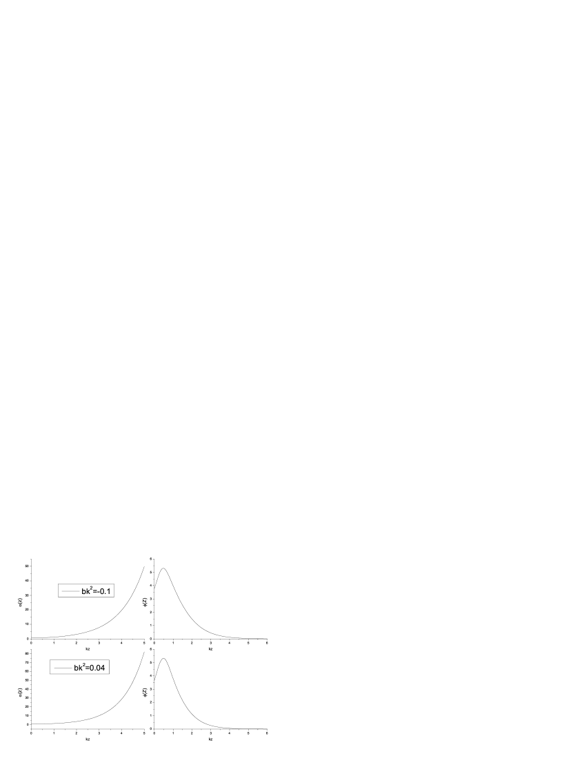
Figure 1: The warp factor $a(z)$ and the scalar field $\phi(z)$, as a function of kz, for $\xi=\xi_{c}$, $\hat{\sigma}=5$, $\hat{\lambda}=0.01$ for two values of $\hat{b}$: $\hat{b}=-0.1$ (upper panel) and $\hat{b}=0.04$ (down panel). The values for $\sigma$ and $\Lambda$ do not satisfy the fine tuning of the RS-model.

In the case of $5D$ conformal coupling $\xi_{c}=3/16$ and $\hat{b}=0$, as we have already mentioned in [9], the warp factor $a(z)$ is of the order of unity in a small region near the brane (starts with $a^{\prime}(0)$ negative) and increases exponentially ($a(z)\rightarrow e^{kz}$), as $z\rightarrow+\infty$, or equivalent the space-time is $AdS_{5}$ asymptotically, while the scalar field $\phi(z)$ is nonzero on the brane (in the region where the warp factor is almost constant) and tends rapidly to zero for large $z$.

In Fig. 1 we see that the above mentioned behavior for the warp factor and the scalar field remains, even when the Gauss-Bonnet term is present. In particular we have plotted the warp factor $a(z)$ and the scalar field $\phi(z)$, as a function of z, for $\xi=\xi_{c}$, for two values of $\hat{b}$: $\hat{b}=-0.1$ and $\hat{b}=0.04$.

A complete investigation of the spectrum of the solutions of the model is quite complicated, however we will try to give a description. We have checked, that for $\hat{b}<0$, the algebraic system of Eqs. (17) and (18) (junction conditions) has only one real solution, which corresponds to a warp factor and a scalar field profile, of the form which is plotted in the upper panel of Fig. 1. On the other hand, for $0<\hat{b}\leq\hat{b}_{c3}$ ($\hat{b}_{c3}=0.16$), the algebraic system of Eqs. (17) and (18) has three real solutions which correspond to three static solutions of the Einstein equations. For $0<\hat{b}<\hat{b}_{c1}$ ($\hat{b}_{c1}=0.1227$) the two of them are of the form of the down panel of Fig. 1 ($Ads_{5}$ in the bulk), and the third has a warp factor which vanishes in finite proper distance $z$ and $\phi(z)$ tends to infinity there (or equivalently it has a naked singularity in the bulk). In the short interval $\hat{b}_{c1}<\hat{b}<\hat{b}_{c2}$ ($\hat{b}_{c2}=0.1250$) only one of the solutions is of the form of the down panel of Fig. 1, and the other two exhibit naked singularities. For $\hat{b}_{c2}<\hat{b}\leq 0.16$ we have three solutions with naked singularities. Finally, for $\hat{b}>0.16$ the algebraic system of Eqs. (17) and (18) has only one real solution, which exhibits a naked singularity in the bulk.

The above presented analysis is valid for a special choice of the free parameters of the model ($\xi=\xi_{c}$, $\hat{\sigma}=5$, $\hat{\lambda}=0.01$). For a different choice the analysis of the spectrum of the solutions is quite similar. For example, in the case of ($\xi=\xi_{c}$, $\hat{\sigma}=2$, $\hat{\lambda}=0.01$), we obtain that $\hat{b}_{c1}=0.1247$ and $\hat{b}_{c2}=0.1250$. Note that the second critical value $\hat{b}_{c2}$ is almost independent from the value of brane tension $\hat{\sigma}$. For large $\hat{b}$ ($\hat{b}>\hat{b}_{c3}$, $\hat{b}_{c3}=1$ ) the model has only one solution with a naked singularity in the bulk.

In the case of a zero tension brane $\hat{\sigma}=0,\hat{\lambda}=0.01$ we have also solutions of the form we described above, with $\phi$ concentrated around zero $(z=0)$ and the space-time is $AdS_{5}$ asymptotically. For $0<\hat{b}<0.1250$ we have three distinct solutions. Two of them are of the form of Fig. 1 and the third exhibits a naked singularity, with a zero warp factor in finite distance and infinite scalar field. Note that the first of the nonsingular solutions is smooth, while the second exhibits an effectively negative brane tension due to the discontinuous first derivative of the scalar field for $z=0$. However, if $\hat{b}$ exceeds the critical value $\hat{b}_{c}=0.1250$ we obtain three solutions which suffer from naked singularities in finite proper distance in the bulk with infinite Ricci scalar. Note that the two critical values $\hat{b}_{c1}$ and $\hat{b}_{c2}$ which are different in the case of the nonzero tension coincide in the case of a zero tension brane $\hat{\sigma}=0$, also $\hat{b}_{c3}$ goes to infinity.

3.2 Class (a) ($\xi<0$)

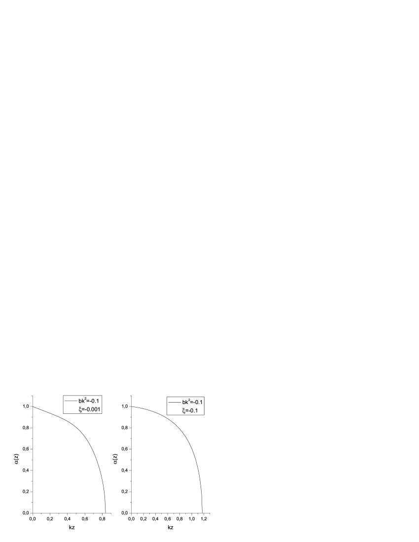
Figure 2: The warp factor $a(z)$, as a function of kz, for $\hat{b}=-0.1$ , $\hat{\sigma}=6$, $\hat{\lambda}=0.01$, for two values of $\xi$: $\xi=-0.001$ (left-hand panel) and $\xi=-0.1$ (right-hand panel). The values for $\sigma$ and $\Lambda$ satisfy the fine tuning of the RS-model.

The solutions for $\xi<0$, as we have seen in our previous paper of Ref. [9], exhibit a naked singularity (in particular the warp factor becomes zero in finite proper distance in the bulk), while the scalar field tends to infinity near the singularity.

It is believed that higher order gravity may incorporate quantum gravity effects which are important when a singularity appears in a solution of Einstein equations. The question that arises is whether Gauss-Bonnet gravity can resolve the naked singularities we obtained in [9].

In order to answer the above question, we examined a wide range of the parameter space of the model, with $\xi<0$, and we found that Gauss-Bonnet gravity can not overcome the singularity in a satisfactory way.

A characteristic behavior for the solutions is presented in Fig. 2, where we have plotted the warp factor $a(z)$, as a function of kz, for $\hat{b}=-0.1$ , $\hat{\sigma}=6$, $\hat{\lambda}=0.01$, and for two values of $\xi$: $\xi=-0.001$ (left-hand panel) and $\xi=-0.1$ (right-hand panel). We see that naked singularity in the bulk remains, even when the coupling $\hat{b}$ possesses a nonzero value. Note that the scalar field tends to infinity near the naked singularity. The warp factor for $\hat{b}=0$ is presented in Figs. (1) and (2) in Ref. [9]. If we compare with the case of nonzero $\hat{b}$ of Fig. 2 in this work, we see that the singularity points are only slightly displaced. We have examined also other values of negative $\hat{b}$, and we observed that for any negative $\hat{b}$ the solutions are of the form we described above.

For positive $\hat{b}$ we see that the algebraic system of equations (13), (17) and (18) has one or more real solutions. Even in this case we cannot avoid naked singularities in the bulk. However, these new singularities are of a different nature from the one we described above. In particular in this case, the second derivative of the warp factor (or the Ricci scalar) tends to infinity in finite proper distance in the bulk, while the warp factor, the scalar field and the first derivative of the warp factor tend to finite values.

For zero tension branes $\hat{\sigma}=0$ we observe the same behavior with that described above. For $\hat{b}\leq 0$ we have one singular solution with a warp factor which tends to zero, while for $\hat{b}>0$ we have only one singular solution with nonzero warp factor but infinite Ricci scalar.

3.3 Class (b) ($\xi>\xi_{c}$)

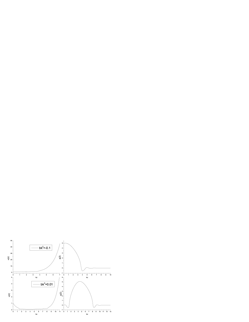
Figure 3: The warp factor $a(z)$, as a function of kz, for $\xi=1+\xi_{c}$, $\hat{\sigma}=6$, $\hat{\lambda}=0.01$, for two values of $\hat{b}$: $\hat{b}=-0.1$ (upper panel) and $\hat{b}=0.01$ (down panel). The values for $\sigma$ and $\Lambda$ satisfy the fine tuning of the RS-model.

For $\hat{b}=0$ and $\xi>\xi_{c}$, we had obtained a different class of numerical solutions in Ref. [9]. In this case the warp factor $a(z)$ is of the order of unity in a small region near the brane and increases exponentially ($a(z)\rightarrow e^{kz}$), as $z\rightarrow+\infty$ (or equivalently the space-time is asymptotically $AdS_{5}$), while the scalar field $\phi(z)$ is nonzero on the brane (in a rather small region near the axes origin where the warp factor remains constant), and for $kz>>1$ tends rapidly to zero.

The question that arises is, how these solutions are modified when a Gauss-Bonnet term is turned on. As we see in the upper panel of Fig. 3, for $\hat{b}=-0.1$, the features of the solution remain the same with those for $\hat{b}=0$. In general, for $\hat{b}<0$, we have only one static solution of the form we described. We have checked numerically that for $0<\hat{b}<\hat{b}_{c1}$ ($\hat{b}_{c1}=0.0106$) the model possesses two static solutions which are asymptotically $AdS_{5}$. The first of them is of the previously described form, while the second has the same profile with the first, but it is translated to a finite proper distance in the bulk, at it is presented in the down panel of Fig. 2. For $\hat{b}_{c1}<\hat{b}<\hat{b}_{c2}$ ($\hat{b}_{c2}=0.0192$) we have also two solutions, but only one is of the form we described above, while the other exhibits a naked singularity. For $\hat{b}>\hat{b}_{c2}$ we obtain one or more singular solutions depending on the value of $\hat{b}$.

3.4 Class (c) ($0<\xi<\xi_{c}$)

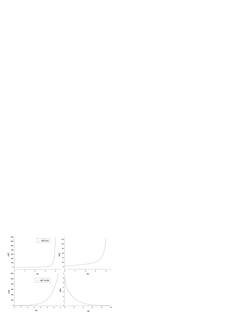
Figure 4: The warp factor $a(z)$ and the scalar field $\phi(z)$, as a function of kz, for $\xi=0.1$, $\hat{\sigma}=6$, $\hat{\lambda}=0.01$, for two values of $\hat{b}$: $\hat{b}=0.5$ (upper panel) and $\hat{b}=-0.04$ (down panel). In the case of $\hat{b}=0.5$ we have naked singularity at $z_{s}=0.42$ in the bulk.

In the absence of the Gauss-Bonnet term ($\hat{b}=0$) and for $0<\xi<\xi_{c}$ the warp factor $a(z)$ and the scalar field $\phi(z)$ tend rapidly to infinity near a singular point in the bulk, like the upper panel of Fig. 4 (for details see Ref. [9]).

We will present an investigation of the spectrum of the static solutions of the model in the case of a specific choice of the free parameters of the model $\xi=0.1$, $\hat{\sigma}=6$ and $\hat{\lambda}=0.01$. For $0<\hat{b}<\hat{b}_{c1}$ ($\hat{b}_{c1}=0.0938$) we have two solutions with singular behavior in the bulk. The first of them exhibits the behavior we described for $\hat{b}=0$, like the upper panel of Fig. 4, and the other has an infinite second derivative of the warp factor, while the functions $a(z)$, $a^{\prime}(z)$ and $\phi(z)$ are finite near the singular point. For $\hat{b}>\hat{b}_{c1}$ we obtain only one solution of the form the upper panel of Fig. 4. In the case of negative $\hat{b}$ and $\hat{b}_{c2}<\hat{b}<0$ ($\hat{b}_{c2}=-0.0485$) we obtain three distinct solutions: a) Singular solutions where the warp factor $a(z)$ vanishes in finite proper distance in the bulk, b) Singular solutions where the second derivative of the warp factor tends to infinity, while the functions $a(z)$, $a^{\prime}(z)$ and $\phi(z)$ are finite near the singular point in the bulk and c) Nonsingular solutions with a warp factor $a(z)$ which increases exponentially ($a(z)\rightarrow e^{kz}$), as $z\rightarrow+\infty$ and a scalar field $\phi(z)$ which is nonzero on the brane, and for $kz>>1$ tends rapidly to zero, see the down panel of Fig. 4. For $\hat{b}_{c3}<\hat{b}<\hat{b}_{c2}$ ($\hat{b}_{c3}=-0.0536$) we have three singular solutions, and for $\hat{b}<\hat{b}_{c3}$ we have only one singular solution.

In general, we observe a similar investigation for other values of the free parameters of the model. In particular, in the case of $\hat{\sigma}=0$ we obtain one singular solution of the form of the upper panel of Fig. 4, for all the values of the Gauss-Bonnet coupling $\hat{b}$.

4 Conclusions and discussion

We considered brane world models with an additional Gauss-Bonnet term in the presence of a massless bulk scalar field which interacts non-minimally with gravity, via a possible interaction term of the form $-\frac{1}{2}\xi R\phi^{2}$. We developed a numerical approach for the solution of the Einstein equations with the scalar field, and we studied the spectrum of the static solutions, in the case of a $\lambda\phi^{4}$ potential, for several values of the free parameters of the model. We obtained that the existence of the Gauss-Bonnet term does not change significantly the solutions we found in our previous work [9], in appropriate regions of the Gauss-Bonnet coupling $\hat{b}$. Outside these regions the solutions always suffers from naked singularities at finite proper distance in the bulk. In general the spectrum of the solutions is characterized from naked singularities except for three cases: i) $\xi>\xi_{c}$ and $\hat{b}<\hat{b}_{c}$ (unstable solutions against scalar field perturbations with a tachyonic spectrum), ii) $\xi=\xi_{c}$ and $\hat{b}<\hat{b}_{c}$ (stable solutions against scalar field perturbations with a continuous spectrum of positive energies) and iii) $0<\xi<\xi_{c}$ and $\hat{b}_{c}<\hat{b}<0$ (stable solutions against scalar field perturbations with a discrete spectrum of positive energies). Note, that the third case of stable solutions is new and does not appear when $\hat{b}$ is equal to zero. Furthermore these solutions share the same properties: $a(z)$ increases exponentially with $z$, and tends to an $AdS_{5}$ space-time asymptotically, while $\phi(z)$ is nonzero near the brane and vanishes rapidly when $z$ is increasing. The brane at $z=0$ has a positive (or zero) brane tension, and the cosmological constant in the bulk is negative. We note, that in the presence of the Gauss-Bonnet term we obtain solutions which are $AdS_{5}$ asymptotically even with positive bulk cosmological constant, but we have not present our study in this case.

Finally, it would be interesting to discuss if the solutions we obtained can be used for the construction of a more realistic brane world model. The main motivation to consider these models was the observation that the interaction term $-\frac{1}{2}\xi R\phi^{2}$ can be interpreted as a mass term, with an effective mass $m^{2}_{eff}=\xi R$. In the case of the second RS-model we obtain that $R=16k\delta(z)-20k^{2}$, and we see, that for negative $\xi$, the effective mass term is negative on the brane and positive in the bulk. This implies an instability of the RS-vacuum near the brane. As we argued in Ref. [10], we expected static stable solutions with a warp factor similar with that of RS-model, and a scalar field vacuum with nonzero value on the brane and zero value in the bulk. These kind of solutions incorporate a layered-phase mechanism for the localization of Standard-Model particles on the brane. This mechanism is based on the idea of the construction of a gauge field model which exhibits a non-confinement phase on the brane and a confinement phase on the bulk. Thus gauge fields, and more generally fermions and bosons with gauge charge, can not escape into the bulk unless we give them energy greater than the mass gap $\Lambda_{G}$, which emerges from the nonperturbative confining dynamics of the gauge field model in the bulk. For an extensive discussion see [10].

In [9] we solved the Einstein equations and we found that there not solutions with the profile we described above for $\xi<0$. However we obtained a class of stable solution, for $\xi=\xi_{c}$ which may be physically interesting. In particular, the warp factor $a(z)$, for this class of solutions, is of the order of unity near the brane and increases exponentially ($a(z)\sim e^{k|z|}$ ), as $z\rightarrow\pm\infty$, while the scalar field $\phi(z)$ is nonzero on the brane and tends rapidly to zero in the bulk. The model is completed if we include a second positive tension brane with $\sigma^{\prime}/k=6$, in a position $z_{c}$ where the scalar field vacuum is practically zero. This two-brane set up is very similar to the well known RS1-model. In analogy with the RS1-model, we will assume that the standard model particles live in the effectively negative tension brane , or visible brane. The advantage of this model is that it incorporates a layered-phase mechanism for the localization of standard model particles on the visible brane, and analyzed in detail in Ref. [9].

In this paper we generalize our previous works by considering brane-models with an additional Gauss-Bonnet term and a bulk scalar field nonminimally coupled with gravity. As we have already mentioned the addition of the Gauss-Bonnet term has not a significant impact to the spectrum of the model, and gives solutions with the same features as the model without the Gauss-Bonnet term. However this model exhibits solutions of the interesting form we described in the previous paragraph, even when $\xi\neq\xi_{c}$. In particular these solutions appear when $0<\xi<\xi_{c}$ and $\hat{b}_{c}<\hat{b}<0$, and can be used for the construction of realistic brane world models, as we describe above.

We would like to note that in the phenomenological studies in [16] the same model, with an additional Gauss-Bonnet term and a bulk scalar field nonminimally coupled with gravity, is considered for $\xi<0$, however the authors of this paper do not take into account the back reaction of the scalar field to the RS vacuum. We think that is important for the phenomenological applications to have a stable background solution, for the complete Einstein equations and the scalar field.

5 Acknowledgements

We are grateful to Professors A. Kehagias and G. Koutsoumbas for reading and commenting on the manuscript. We also thank Professors C. Charmousis, I. P. Neupane, E Papantonopoulos and J. Zanelli for important discussions and comments. This work is supported by the EPEAEK programme ”Pythagoras” and co-founded by the European-Union (75${}^{\circ}/_{\circ}$) and the Hellenic state (25${}^{\circ}/_{\circ}$).

References

- [1] K. Akama, ”Pregeometry” in Lecture Notes in Physics, 176, Gaquge Theory and Gravitation, Proceedings, Nara, 1982, edited by K. Kikkawa, N. Nakanishi and H. Nariai, 267-271 (Springer-Verlag, 1983); Prog.Theor. Phys. 60, 1900 (1978); 78, 184 (1987); 79, 1299 (1988); 80, 935 (1988);
- [2] V.A. Rubakov and M.E. Shaposhnikov, Phys. Lett. B125:136-138, 1983; Phys. Lett. B125:139, 1983.
- [3] N. Arkami-Hamed, S. Dimopoulos and G. Dvali, Phys. Lett. B429 (1998) 263; I. Antoniadis, N. Arkami-Hamed, S. Dimopoulos and G. Dvali, Phys. Lett. B436 (1998) 257;
- [4] L. Randall and R. Sundrum, Phys. Rev. Lett. 83 (1999) 3370; Phys. Rev. Lett. 83 (1999) 4690;
- [5] N. Arkani-Hamed, S. Dimopoulos, N. Kaloper and R. Sundrum, Phys. Lett. B 480 (2000) 193.
- [6] V. A. Rubakov, Phys. Usp. 44 (2001) 871;
- [7] A. Kehagias and K. Tamvakis, Phys. Lett. B 504 (2001) 38.
- [8] M. Giovannini, Non-topological gravitating defects in five-dimensional anti-de Sitter space,hep-th/0607229;
- [9] K. Farakos and P. Pasipoularides, Phys. Rev. D73 (2006) 084012.
- [10] K. Farakos and P. Pasipoularides, Phys. Lett. B 621, (2005) 224-232.
- [11] G. Dvali and M. Shifman, Phys. Lett. B 396 (1997) 64.
- [12] C.P. Korthals-Altes, S. Nicolis and J. Prades, Phys. Lett. B316 (1993), 339; A. Hulsebos, C.P. Korthals-Altes and S. Nicolis, Nucl. Phys. B450 (1995) 437.
- [13] P. Dimopoulos, K. Farakos, A. Kehagias and G. Koutsoumbas, Nucl. Phys. B 617 (2001) 237-252; P. Dimopoulos, K. Farakos, G. Koutsoumbas, Phys. Rev. D65 (2002) 074505; P. Dimopoulos, K. Farakos, Phys. Rev. D70 (2004) 045005; P.Dimopoulos, K.Farakos and S.Vrentzos, The 4-D Layer Phase as a Gauge Field Localization: Extensive Study of the 5-D Anisotropic U(1) Gauge Model on the Lattice, hep-lat/0607033.
- [14] M. Laine, H.B. Meyer, K. Rummukainen, M. Shaposnikov, JHEP 0404 (2004) 027.
- [15] A. Flachi and D. J. Toms, Phys Lett. B 491, (2000) 157
- [16] H. Davoudiasl, B. Lillie and T. G. Rizzo, Off-the-Wall Higgs in the Universal Randal-Sundrum Model, JHEP 0608 (2006) 042.
- [17] C. Bogdanos, A. Dimitriadis and K. Tamvakis, Phys.Rev. D74 (2006) 045003; C. Bogdanos, Exact Solutions in 5-D Brane Models With Scalar Fields, hep-th/0609143.
- [18] C. Bogdanos, A. Dimitriadis, K. Tamvakis, Brane Cosmology with a Non-Minimally Coupled Bulk-Scalar Field, hep-th/0611181.
- [19] Alexey S. Mikhailov, Yuri S. Mikhailov, Mikhail N. Smolyakov and Igor P. Volobuev, Class. Quantum Grav. 24 (2007) 231-242.
- [20] Rodrigo Aros, Mauricio Contreras, Rodrigo Olea, Ricardo Troncoso and Jorge Zanelli, Phys.Rev.Lett. 84 (2000) 1647-1650; Rodrigo Olea, JHEP 0506 (2005) 023.
- [21] Jihn E. Kim, Bumseok Kyae and Hyun Min Lee, Phys.Rev. D62 (2000) 045013; Jihn E. Kim, Bumseok Kyae and Hyun Min Lee, Nucl.Phys. B582 (2000) 296-312.
- [22] Y. M. Cho, Ishwaree P. Neupane and P. S. Wesson, Nucl.Phys. B621 (2002) 388-412; Y. M. Cho and Ishwaree P. Neupane, Int.J.Mod.Phys. A18 (2003) 2703-2727; Ishwaree P. Neupane, Phys.Lett. B512 (2001) 137-145;
- [23] Christos Charmousis, Jean-Francois Dufaux, Phys.Rev. D70 (2004) 106002.
- [24] Shin’ichi Nojiri and Sergei D. Odintsov, JHEP 0007 (2000) 049.
- [25] N. M. Mavromatos and J. Rizos, Phys. Rev. D62 (2000) 124004; Int.J.Mod.Phys. A18 (2003) 57-84;
- [26] Ishwaree P. Neupane, JHEP 0009 (2000) 040;
- [27] Pierre Binetruy, Christos Charmousis, Stephen C Davis and Jean-Francois Dufaux, Phys.Lett. B544 (2002) 183-191; Christos Charmousis, Stephen C. Davis, Jean-Francois Dufaux, JHEP 0312 (2003) 029;
- [28] Massimo Giovannini, Phys.Rev. D64 (2001) 124004; Kink-antikink, trapping bags and five-dimensional Gauss-Bonnet gravity, hep-th/0609136; Gravitating multidefects from higher dimensions, hep-th/0612104.
- [29] Christos Charmousis and Jean-Francois Dufaux, Class.Quant.Grav. 19 (2002) 4671-4682
- [30] G. Kofinas, R. Maartens, E. Papantonopoulos, JHEP 0310 (2003) 066; Richard A. Brown, Roy Maartens, Eleftherios Papantonopoulos and Vassilis Zamarias, JCAP 0511 (2005) 008.
- [31] S. M. Carroll, Spacetime and geometry, Addison Wesley 2004.