PUPT-2209, DUKE-CGTP-06-03

hep-th/0610007

D-branes at Singularities,
Compactification, and Hypercharge

Matthew Buican^a, Dmitry Malyshev^a,, David R. Morrison^b,c,
Herman Verlinde^a and Martijn Wijnholt^a,d

^a Department of Physics, Princeton University, Princeton, NJ 08544
^b Center for Geometry and Theoretical Physics, Duke University, Durham, NC 27708
^c Departments of Physics and Mathematics, Univ. of California, Santa Barbara, CA 93106
^d Max-Planck-Institut für Gravitationsphysik, Albert-Einstein-Institut, Potsdam, Germany

We report on progress towards the construction of SM-like gauge theories on the world-volume of D-branes at a Calabi–Yau singularity. In particular, we work out the topological conditions on the embedding of the singularity inside a compact CY threefold, that select hypercharge as the only light $U(1)$ gauge factor. We apply this insight to the proposed open string realization of the SM of hep-th/0508089, based on a D3-brane at a $dP_{8}$ singularity, and present a geometric construction of a compact Calabi–Yau threefold with all the required topological properties. We comment on the relevance of D-instantons to the breaking of global $U(1)$ symmetries in D-brane models.

1. Introduction

D-branes near Calabi–Yau singularities provide open string realizations of an increasingly rich class of gauge theories [1, 2, 3]. Given the hierarchy between the Planck and TeV scale, it is natural to make use of this technology and pursue a bottom-up approach to string phenomenology, that aims to find Standard Model-like theories on D-branes near CY singularities. In this setting, the D-brane world-volume theory can be isolated from the closed string physics in the bulk via a formal decoupling limit, in which the string and 4-d Planck scale are taken to infinity, or very large. The clear advantage of this bottom-up strategy is that it separates the task of finding local realizations of SM-like models from the more difficult challenge of finding fully consistent, realistic string compactifications.

In scanning the space of CY singularities for candidates that lead to realistic gauge theories, one is aided by the fact that all gauge invariant couplings of the world-volume theory are controlled by the local geometry; in particular, symmetry breaking patterns can be enforced by appropriately dialing the volumes of compact cycles of the singularity. Several other properties of the gauge theory, however, such as the spectrum of light $U(1)$ vector bosons and the number of freely tunable couplings, depend on how the local singularity is embedded inside the full compact Calabi–Yau geometry.

In this paper we work out some concrete aspects of this program. We begin with a brief review of the general set of ingredients that can be used to build semi-realistic gauge theories from branes at singularities. Typically these local constructions lead to models with extra $U(1)$ gauge symmetries beyond hypercharge. As our first new result, we identify the general topological conditions on the embedding of a CY singularity inside a compact CY threefold, that determines which $U(1)$-symmetry factors survive as massless gauge symmetries. The other $U(1)$ bosons acquire a mass of order of the string scale. The left-over global symmetries are broken by D-brane instantons.

In the second half of the paper, we apply this insight to the concrete construction of an SM-like theory given in [5], based on a single D3-brane near a suitably chosen del Pezzo 8 singularity. We specify a simple topological condition on the compact embedding of the $dP_{8}$ singularity, such that only hypercharge survives as the massless gauge symmetry. To state this condition, recall that the 2-homology of a $dP_{8}$ surface is spanned by the canonical class $K$ and eight 2-cycles $\alpha_{i}$ with intersection form $\alpha_{i}\cdot\alpha_{j}=-A_{ij}$ with $A_{ij}$ the Cartan matrix of $E_{8}$. With this notation, our geometric proposal is summarized as follows:

The world-volume gauge theory on a single D3-brane near a del Pezzo 8 singularity embedded in a compact Calabi-Yau threefold with the following geometrical properties:
    (i) the two 2-cycles $\alpha_{1}$ and $\alpha_{2}$ are degenerate and form a curve of $A_{2}$ singularities
    (iii) all 2-cycles except $\alpha_{4}$ are non-trivial within the full Calabi-Yau three-fold
has, for a suitable choice of Kähler moduli, the gauge group and matter content of the SSM

	$Q_{i}$	$u_{i}^{c}$	$d_{i}^{c}$	$\ell_{i}$	$e_{i}^{c}$	$\nu_{i}^{c}$	$H_{i}^{u}$	$H_{i}^{d}$
$SU(3)_{C}$	3	$\bar{\bf{3}}$	$\bar{\bf{3}}$	1	1	1	1	1
$SU(2)_{L}$	2	1	1	2	1	1	2	2
$U(1)_{Y}$	1/6	$-2/3$	1/3	$-1/2$	1	0	1/2	$-1/2$

Table 1: The matter content of our D-brane model. $i$ counts the 3 generations

shown in Table 1, except for an extended Higgs sector (with 2 pairs per generation):

More details of this proposal are given in section 4. In section 5, we present a concrete geometric recipe for obtaining a compact CY manifold with all the required properties.

2. General Strategy

We begin with a summary our general approach to string phenomenology. In subsection 2.1, we give a quick recap of some relevant properties of D-branes at singularities. The reader familiar with this technology may wish to skip to subsection 2.2.

2.1. D-branes at a CY singularity

D-branes near Calabi–Yau singularities typically split up into so-called fractional branes. Fractional branes can be thought of as particular bound state combinations of D-branes, that wrap cycles of the local geometry. In terms of the world-sheet CFT, they are in one-to-one correspondence with allowed conformally invariant open string boundary conditions. Alternatively, by extrapolating to a large volume perspective, fractional branes may be represented geometrically as particular well-chosen collections of sheaves, supported on corresponding submanifolds within the local Calabi–Yau singularity. For most of our discussion, however, we will not need this abstract mathematical description; the basic properties that we will use have relatively simple topological specifications.

There are many types of CY-singularities, and some are, in principle, good candidates for finding realistic D-brane gauge theories. For concreteness, however, we specialize to the subclass of singularities which are asymptotic to a complex cone over a del Pezzo surface $X$. D-brane theories on del Pezzo singularities have been studied in [5, 6, 7].

A del Pezzo surface is a manifold of complex dimension 2, with a positive first Chern class. Each del Pezzo surface other than ${\mathbb{P}}^{1}\times{\mathbb{P}}^{1}$ can be represented as ${\mathbb{P}}^{2}$ blown up at $n\leq 8$ generic points; such a surface is denoted by ${dP_{n}}$ and sometimes called “the $n$-th del Pezzo surface”. By placing an appropriate complex line bundle (the “anti-canonical bundle”) over $X={dP_{n}}$, one obtains a smooth non-compact Calabi–Yau threefold. If we then shrink the zero section of the line bundle to a point, we get a cone over $X$, which we will call the conical del Pezzo $n$ singularity and denote by $Y_{0}$. (More general del Pezzo singularities are asymptotic to $Y_{0}$ near the singular point.) To specify the geometry of $Y_{0}$, let $ds_{X}^{2}=h_{a\bar{b}}dz^{a}dz^{\bar{b}}$ be a Kähler-Einstein metric over the base $X$ with $R_{a\bar{b}}=6h_{a\bar{b}}$ and first Chern class $\omega_{a\bar{b}}=6iR_{a\bar{b}}$. Introduce the one-form $\eta={1\over 3}d\psi+\sigma$ where $\sigma$ is defined by $d\sigma=2\omega$ and $0<\psi<2\pi$ is the angular coordinate for a circle bundle over the del Pezzo surface. The Calabi–Yau metric can then be written as follows

$$ds^{2}_{Y}=dr^{2}+r^{2}\eta^{2}+r^{2}ds^{2}_{X}$$ (1)

For the non-compact cone, the $r$-coordinate has infinite range. Alternatively, we can think of the del Pezzo singularity as a localized region within a compact CY manifold, with $r$ being the local radial coordinate distance from the singularity. We will consider both cases.
$\begin{array}[]{cc}\noindent\parbox{264.6107pt}{ ${}$ \ \ The del Pezzo surface $X$ forms a four-cycle within the full three-manifold $Y$, and itself supports several non-trivial two-cycles. Now, if we consider IIB string theory on a del Pezzo singularity, we should expect to find a basis of fractional branes that spans the complete homology of $X$: the del Pezzo 4-cycle itself may be wrapped by any number of D7-branes, any 2-cycle within $X$ may be wrapped by one or more D5 branes, and the point-like D3-branes occupy the 0-cycle within $X$. The allowed fractional branes, however, typically do not correspond to single branes wrapped on some given cycle, but rather }\parbox{199.16928pt}{\ \ \ \ \ \ \ \ \leavevmode\hbox{\epsfbox{dfive.eps}} }\end{array}$
to particular bound states ${\mathsf{F}}_{\!s}$, each characterized by a charge vector of the form

$${\rm ch}({\mathsf{F}}_{\!s})=(\,r_{\!s},\,p_{s}^{\,{\mbox{\scriptsize\sc a}}},\,q_{s}\,)$$ (2)

Here $r_{\!s}\!={\rm rk}({\mathsf{F}}_{\!s})$ is the rank of the fractional brane ${\mathsf{F}}_{s}$, and is equal to the D7-brane wrapping number around $X$. The number $q_{s}\!=\!{\rm ch}_{2}({\mathsf{F}}_{\!s})$ is the 2nd Chern character of ${\mathsf{F}}_{\!s}$ and counts the D3-brane charge. Finally, the integers $p_{s}^{\,{\mbox{\scriptsize\sc a}}}$ are extracted from the first Chern class of ${\mathsf{F}}_{\!s}$ via

$$p_{s}^{\mbox{\scriptsize\sc a}}=\int_{\alpha_{\mbox{\scriptsize\sc a}}}\!c_{1}({\mathsf{F}}_{\!s})$$ (3)

where $\alpha_{\mbox{\scriptsize\sc a}}$ denotes an integral basis of $H_{2}(X)$. Geometrically, $p_{s}^{\,{\mbox{\scriptsize\sc a}}}$ counts the number of times the D5-brane component of ${\mathsf{F}}_{\!s}$ wraps the 2-cycle $\alpha_{\mbox{\scriptsize\sc a}}$.

For a given geometric singularity, it is a non-trivial problem to find consistent bases of fractional branes that satisfy all geometric stability conditions. For del Pezzo singularities, a special class of consistent bases are known, in the form of so-called exceptional collections [20, 6, 7]. These satisfy special properties, that in particular ensures the absence of adjoint matter in the world-volume gauge theory, besides the gauge multiplet. The formula for the intersection product between two fractional branes ${\mathsf{F}}_{i}$ and ${\mathsf{F}}_{j}$ of an exceptional collection reads

$$\#({\mathsf{F}}_{i},{\mathsf{F}}_{j})={\rm rk}({\mathsf{F}}_{i})\,{\rm deg}({\mathsf{F}}_{j})-{\rm rk}({\mathsf{F}}_{j})\,{\rm deg}({\mathsf{F}}_{i})\,\equiv\,\chi_{ij}$$ (4)

Here the degree of ${\mathsf{F}}_{i}$ is given by ${\rm deg}({\mathsf{F}}_{i})\!=\!-c_{1}({\mathsf{F}}_{i})\!\cdot\!K$ with $K$ the canonical class on $X$. It equals the intersection number between the D5 component of ${\mathsf{F}}_{i}$ and the del Pezzo surface. The intersection number $\chi_{ij}$ governs the number of massless states of open strings that stretch between the two fractional branes ${\mathsf{F}}_{i}$ and ${\mathsf{F}}_{j}$.

The world-volume theory on D-branes near a CY singularity takes the form of a quiver gauge theory. For exceptional collections, the rules for drawing the quiver diagram are:  (i)  draw a single node for every basis element ${\mathsf{F}}_{i}$ of the collection, (ii) connect every pair of nodes with $\chi_{ij}>0$ by an oriented line with multiplicity $\chi_{ij}$. Upon assigning a multiplicity $n_{i}$ to each fractional brane ${\mathsf{F}}_{i}$, one associates to the quiver diagram a quiver gauge theory. The gauge theory has a $U(|n_{i}|)$ gauge group factor for every node ${\mathsf{F}}_{i}$, as well as $\chi_{ij}$ chiral multiplets in the bi-fundamental representation $(n_{i},\bar{n}_{j})$. The multiplicities $n_{i}$ can be freely adjusted, provided the resulting world volume theory is a consistent ${\cal N}\!=\!1$ gauge theory, free of any non-abelian gauge anomalies.

Absence of non-abelian gauge anomalies is ensured if at any given node, the total number of incoming and outgoing lines (each weighted by the rank of the gauge group at the other end of the line) are equal:

$$\sum_{j}\chi_{ij}\,n_{j}=0\,.$$ (5)

This condition is automatically satisfied if the configuration of fractional branes constitute a single D3-brane, in which case the multiplicities $n_{i}$ are such that $\sum_{i}n_{i}\,{\rm ch}({\mathsf{F}}_{i})\!=\!(\,0,0,1\,)$. In general, however, one could allow for more general configurations, for which the charge vectors add up to some non-trivial fractional brane charge.

For a given type of singularity, the choice of exceptional collection is not unique. Different choices are related via simple basis transformations, known as mutations [20]. However, only a subset of all exceptional collections, that can be reached via mutations, lead to consistent world-volume gauge theories. The special mutations that act within the subset of physically relevant collections all take the form of Seiberg dualities [6, 7]. Which of the Seiberg dual descriptions is appropriate is determined by the value of the geometric moduli that determine the gauge theory couplings.

2.2. Symmetry breaking towards the SSM

To find string realizations of SM-like theories we now proceed in two steps. First we look for CY singularities and brane configurations, such that the quiver gauge theory is just rich enough to contain the SM gauge group and matter content. Then we look for a well-chosen symmetry breaking process that reduces the gauge group and matter content to that of the Standard Model, or at least realistically close to it. When the CY singularity is not isolated, the moduli space of vacua for the D-brane theory has several components [3], and the symmetry breaking we need is found on a component in which some of the fractional branes move off of the primary singular point along a curve of singularities (and other branes are replaced by appropriate bound states). This geometric insight into the symmetry breaking allows us to identify an appropriate CY singularity, such that the corresponding D-brane theory looks like the SSM.

The above procedure was used in [5] to construct a semi-realistic theory from a single D3-brane on a partially resolved del Pezzo 8 singularity (see also section 4). The final model of [5], however, still has several extra $U(1)$ factors besides the hypercharge symmetry. Such extra $U(1)$’s are characteristic of D-brane constructions: typically, one obtains one such factor for every fractional brane. As will be explained in what follows, whether or not these extra $U(1)$’s actually survive as massless gauge symmetries depends on the topology of how the singularity is embedded inside of a compact CY geometry.

In a string compactification, $U(1)$ gauge bosons may acquire a non-zero mass via coupling to closed string RR-form fields. We will describe this mechanism in some detail in the next section, where we will show that the $U(1)$ bosons that remain massless are in one-to-one correspondence with 2-cycles, that are non-trivial within the local CY singularity but are trivial within the full CY threefold. This insight in principle makes it possible to ensure – via the topology of the CY compactification – that, among all $U(1)$ factors of the D-brane gauge theory, only the hypercharge survives as a massless gauge symmetry.

The interrelation between the 2-cohomology of the del Pezzo base of the singularity, and the full CY threefold has other relevant consequences. Locally, all gauge invariant couplings of the D-brane theory can be varied via corresponding deformations of the local geometry. This local tunability is one of the central motivations for the bottom-up approach to string phenomenology. The embedding into a full string compactification, however, typically introduces a topological obstruction against varying all local couplings: only those couplings that descend from moduli of the full CY survive. Their value will need to be fixed via a dynamical moduli stabilisation mechanism.

2.3. Summary

Let us summarize our general strategy in terms of a systematized set of steps:
(i) Choose a non-compact CY singularity, $Y_{0}$, and find a suitable basis of fractional branes ${\mathsf{F}}_{i}$ on it. Assign multiplicities $n_{i}$ to each ${\mathsf{F}}_{i}$ and enumerate the resulting quiver gauge theories.
(ii) Look for quiver theories that, after symmetry breaking, produce an SM-like theory. Use the geometric dictionary to identify the corresponding (non-isolated) CY singularity.
(iii) Identify the topological condition that isolates hypercharge as the only massless $U(1)$. Look for a compact CY threefold, with the right topological properties, that contains ${Y}_{0}$.

In principle, it should be possible to automatize all three of these steps and thus set up a computer-aided search of SM-like gauge theories based on D-branes at CY singularities.

3. $U(1)$ Masses via RR-couplings

The quiver theory of a D-brane near a CY singularity typically contains several $U(1)$-factors, one for each fractional brane. Some of these $U(1)$ vector bosons remain massless, all others either acquire a Stückelberg mass via the coupling to the RR-form fields or get a mass through the Higgs mechanism [1, 18, 19, 12]. We will now discuss the Stückelberg mechanism in some detail.

3.1. The $U(1)$ hypermultiplet

To set notation, we first consider the $U(1)$ gauge sector on a single fractional brane. Let us introduce the two complex variables

$$\tau={\theta\over 2\pi}+i{4\pi\over g^{2}}\,,\qquad\qquad\quad S=\rho+i\zeta\,.$$ (6)

Here $\tau$ is the usual $SL(2,{\mathbb{Z}})$ covariant complex coupling, that governs the kinetic terms of the $U(1)$ gauge boson via (omitting fermionic terms)

$${\rm Im}\int\!d^{2}\theta\,{\tau\over 8\pi}\,W_{\alpha}W^{\alpha}=-{1\over 4g^{2}}\,F\wedge*F+{\theta\over 32\pi^{2}}\,F\wedge F$$ (7)

The field $S$ in (6) combines a Stückelberg field $\rho$ and a Faillet-Iliopoulos parameter $\zeta$. After promoting $S$ to a chiral superfield, we can write a supersymmetric gauge invariant mass term for the gauge field via [1]

$$\int\!d^{4}\theta\,\frac{1}{4}({\rm Im}(S\!-\!\bar{S}\!-2V))^{2}=\frac{1}{2}(A-d\rho)\!\wedge*(A-d\rho)\;-\,\zeta D.$$ (8)

Here $D$ denotes the auxiliary field of the vector multiplet $V$. Together with the mass term, we observe a Faillet-Iliopoulos term proportional to $\zeta$.

The complex parametrization (6) of the D-brane couplings naturally follows from its embedding in type IIB string theory. Without D-branes, IIB supergravity on a Calabi–Yau threefold preserves $\mathcal{N}\!=\!2$ supersymmetry. Closed string fields thus organize in $\mathcal{N}\!=\!2$ multiplets [9, 10]. The four real variables in (6) all fit together as the scalar components of a single hypermultiplet that appears after dualizing two components of the so called double tensor multiplet [11]. Since adding a D-brane breaks half the supersymmetry, the hypermultiplet splits into two complex $\mathcal{N}\!=\!1$ superfields with scalar components $\tau$ and $S$. The hypermultiplet of a single D3-brane derives directly from the 10-d fields, via

$$\tau\! \!=\! \!C_{0}+ie^{-\phi},$$

$$dS\,\! \!=\! \!*d(C_{\it 2}+\tau B_{\it 2})$$ (9)

A $dP_{n}$ singularity $Y_{0}$ supports a total of $n+3$ independent fractional branes, and a typical D-brane theory on $Y_{0}$ thus contains $n+3$ separate $U(1)$ gauge factors. In our geometric dictionary, we need to account for a corresponding number of closed string hypermultiplets.

In spite their common descent from the hypermultiplet, from the world volume perspective $\tau$ and $S$ appear to stand on somewhat different footing: $\tau$ can be chosen as a non-dynamical coupling, whereas $S$ must enter as a dynamical field. In a decoupling limit, one would expect that all closed string dynamics strictly separates from the open string dynamics on the brane, and thus that all closed string fields freeze into fixed, non-dynamical couplings. This decoupling can indeed be arranged, provided the $U(1)$ symmetry is non-anomalous and one starts from a D-brane on a non-compact CY singularity. In this setting, $\tau$ becomes a fixed constant as expected, while $S$ completely decouples, simply because the $U(1)$ gauge boson stays massless.

3.2. Some notation

As before, let $Y_{0}$ be a non-compact CY singularity given by a complex cone over a base $X$. A complete basis of IIB fractional branes on $Y_{0}$ spans the space of compact, even-dimensional homology cycles within $Y_{0}$, which coincides with the even-dimensional homology of $X$. The 2-homology of the $n$-th del Pezzo surface $dP_{n}$ is generated by the canonical class $\alpha_{0}=k$, plus $n$ orthogonal 2-cycles $\alpha_{i}$. Using the intersection pairing within the threefold $Y_{0}$, we introduce the dual 4-cycles $\beta^{\mbox{\scriptsize\sc b}}$ satisfying

$$\qquad\alpha_{\mbox{\scriptsize\sc a}}\cdot\beta^{\mbox{\scriptsize\sc b}}=\delta_{\mbox{\scriptsize\sc a}}^{\mbox{\scriptsize\sc b}}\qquad\quad\mbox{{\scriptsize A, B} {\small$=0,\ldots,n$}}$$ (10)

The cycle $\beta^{0}$, dual to the canonical class $\alpha_{0}$, describes the class of the del Pezzo surface $X$ itself, and forms the only compact 4-cycle within $Y_{0}$. The remaining $\beta$’s are all non-compact and extend in the radial direction of the cone. The degree zero two-cycles $\alpha_{i}$, that satsify $\alpha_{0}\cdot\alpha_{i}=0$, have the intersection form

$$\alpha_{i}\cdot\alpha_{j}=-A_{ij}$$ (11)

where $A_{ij}$ equals minus the Cartan matrix of $E_{n}$. The canonical class has self-intersection $9-n$. In the following we will use the intersection matrix

$$\eta_{{\mbox{\scriptsize\sc a}}{\mbox{\scriptsize\sc b}}}=\left(\begin{array}[]{cc}9-n&0\\[5.69054pt] 0&-A_{ij}\end{array}\right)$$ (14)

and its inverse $\eta^{{\mbox{\scriptsize\sc a}}{\mbox{\scriptsize\sc b}}}$ to raise and lower A-indices.

3.3. Brane action

The 10-d IIB low energy field theory contains the following bosonic fields: the dilaton $\phi$, the NS 2-form $B$, the Kähler 2-form $J$ and the RR $p$-form potentials $C_{p}$, with $p$ even from 0 to 8. (Note that the latter are an overcomplete set, since $dC_{p}=*_{{}_{10}}dC_{8-p}$.) From each of these fields, we can extract a 4-d scalar fields via integration over a corresponding compact cycles within $Y_{0}$. These scalar fields parametrize the gauge invariant couplings of the D-brane theory. Near a CY singularity, however, $\alpha^{\prime}$ corrections may be substantial, and this gauge theory/geometric dictionary is only partially under control. We will not attempt to solve this hard problem and will instead adopt a large volume perspective, in which the local curvature is assumed to be small compared to the string scale. All expressions below are extracted from the leading order DBI action. Moreover, we drop all curvature contributions, as they do not affect the main conclusions. To keep the formulas transparant, we omit factors of order 1 and work in $\ell_{s}=1$ units. For a more precise treatment, we refer to [12].

The D-brane world-volume theory lives on a collection of fractional branes ${\mathsf{F}}_{s}$, with properties as summarized in section 2. Since the fractional branes all carry a non-zero D7 charge $r_{\!s}$, we can think of them as D7-branes, wrapping the base $X$ of the CY singularity $r_{\!s}$ times. We can thus identify the closed string couplings of ${\mathsf{F}}_{\!s}$ via its world volume action, given by the sum of a Born-Infeld and Chern-Simons term via

$$\qquad\mathcal{S}=\int\!e^{-i^{*}_{s}\phi}\sqrt{{\rm det}(i_{s}^{*}\,(G+B)-F_{s})}\,+\int\!\mbox{\large$\sum\limits_{\raisebox{1.42262pt}{\scriptsize$p$}}$}\;i_{s}^{*}C_{p}\;e^{{F}_{s}-i_{s}^{*}B}\,.$$ (15)

Here $i^{*}_{s}$ denotes the pull-back of the various fields to the world-volume of ${\mathsf{F}}_{s}$; it in particular encodes the information of the D7 brane wrapping number $r_{\!s}$. In case the D7 brane wrapping number $r_{\!s}$ is larger than one, we need to replace the abelian field strength $F_{s}$ to a non-abelian field-strength and take a trace where appropriate.

The D5 charges of ${\mathsf{F}}_{s}$ are represented by fluxes of the field strength $F_{\!s}$ through the various 2-cycles within $X$.

$$p_{s}^{\mbox{\scriptsize\sc a}}=\int_{\alpha_{\mbox{\scriptsize\sc a}}}{\rm Tr}(F_{s})$$ (16)

Analogously, the D3-brane charge is identified with the instanton number charge.

$$q_{s}=\int_{X}{1\over 2}\,\!{\rm Tr}(F_{s}\wedge F_{s})$$ (17)

The D5 charges $p_{s{\mbox{\scriptsize\sc a}}}$ are integers, whereas the D3 charge $q_{s}$ may take half-integer values.

The D-brane world volume action, since it depends on the field strength $F_{s}$ via the combination

$${\cal F}_{s}=F_{s}-i^{*}_{s}B\,,$$

is invariant under gauge transformations $B_{\it 2}\to B_{\it 2}+d\Lambda$, $A_{s}\to A_{s}+\Lambda$, with $\Lambda$ any one-form. If $\Lambda$ is single valued, then the fluxes $p_{s}^{\mbox{\scriptsize\sc a}}$ of $F_{s}$ remain unchanged. But the only restriction is that $d\Lambda$ belongs to an integral cohomology class on $Y$. The gauge transformations thus have an integral version, that shifts the integral periods of $B$ into fluxes of $F_{s}$, and vice versa. This integral gauge invariance naturally turns the periods of $B_{\it 2}$ into angular variables. The relevant $B$-periods for us are those along the 2-cycles of the del Pezzo surface $X$

$$b^{\mbox{\scriptsize\sc a}}\! \!=\! \!\int_{\alpha_{\mbox{\scriptsize\sc a}}}\!B.$$ (18)

The integral gauge transformations act on these periods and the D-brane charges via

$$\qquad b^{\mbox{\scriptsize\sc a}} \to b^{\mbox{\scriptsize\sc a}}+n^{\mbox{\scriptsize\sc a}}$$

$$\qquad p_{s}^{\mbox{\scriptsize\sc a}} \to p_{s}^{\mbox{\scriptsize\sc a}}+n^{\mbox{\scriptsize\sc a}}\,r_{s}$$ (19)

$$\qquad q_{s} \to q_{s}-n_{\mbox{\scriptsize\sc a}}\,p_{s}^{{\mbox{\scriptsize\sc a}}}-{\textstyle{1\over 2}}r_{s}n_{\mbox{\scriptsize\sc a}}n^{\mbox{\scriptsize\sc a}}$$

with $n^{\mbox{\scriptsize\sc a}}$ an a priori arbitrary set of integers. These transformations can be used to restrict the $b^{\mbox{\scriptsize\sc a}}$ to the interval between 0 and 1.

Physical observables should be invariant under (S3.Ex3). This condition provides a useful check on calculations, whenever done in a non-manifestly invariant notation. A convenient way to preserve the invariance, is to introduce a new type of charge vector for the fractional branes, obtained by replacing in the definitions (16) and (17) the field strength $F_{s}$ by ${\cal F}_{s}$:

$${\mathsf{Q}}({\mathsf{F}}_{s})=({\bf r}_{s},{\mathsf{p}}_{s{\mbox{\scriptsize\sc a}}},{\mathsf{q}}_{s})\qquad$$ (20)

where ${\bf r}_{s}=r_{s}$ and

$$\qquad{\mathsf{p}}_{s{\mbox{\scriptsize\sc a}}}\!\!\! \!=\! \!p_{s{\mbox{\scriptsize\sc a}}}-r_{s}b_{\mbox{\scriptsize\sc a}}$$

$$\qquad{\mathsf{q}}_{s}\!\! \!=\! \!q_{s}+p_{s}^{\,{\mbox{\scriptsize\sc a}}}\,b_{\mbox{\scriptsize\sc a}}-{\textstyle{1\over 2}}\,r_{s}\,b^{\mbox{\scriptsize\sc a}}b_{\mbox{\scriptsize\sc a}}$$ (21)

The new charges can take any real value, and are both invariant under (S3.Ex3).

The charge vector is naturally combined into the central charge ${\mathsf{Z}}({\mathsf{F}}_{s})$ of the fractional brane ${\mathsf{F}}_{s}$. The central charge is an exact quantum property of the fractional brane, that can be defined at the level of the worldsheet CFT as the complex number that tells us which linear combination of right- and left-moving supercharges the boundary state of the brane preserves. It depends linearly on the charge vector:

$${\mathsf{Z}}({\mathsf{F}}_{s})={\mathsf{\Pi}}\cdot{\mathsf{Q}}({\mathsf{F}}_{s}),$$ (22)

with ${\mathsf{\Pi}}$ some vector that depends on the geometry of the CY singularity.

In the large volume regime, one can show that the central charge is given by the following expression: [14, 15, 16]

$${\mathsf{Z}}({\mathsf{F}}_{s})=\int_{X}\!e^{-i_{s}^{*}(B+iJ)}\,{\rm Tr}(e^{F_{s}})$$ (23)

where $J$ denotes the Kähler class on $Y$. Evaluating the integral gives

$${\mathsf{Z}}({\mathsf{F}}_{s})\! \!=\! \!{\mathsf{q}}_{s}\,-\textstyle{1\over 2}\,{\bf r}_{s}\,\zeta^{\mbox{\scriptsize\sc a}}\zeta_{\mbox{\scriptsize\sc a}}-\,i\,{\mathsf{p}}_{s{\mbox{\scriptsize\sc a}}}\,\zeta^{\mbox{\scriptsize\sc a}}\,,$$ (24)

with

$$\zeta^{\mbox{\scriptsize\sc a}}\! \!=\! \!\int_{\alpha_{\mbox{\scriptsize\sc a}}}J\,.$$ (25)

With this preparation, let us write the geometric expression for the couplings of the fractional brane ${\mathsf{F}}_{\!s}$. From the central charge $Z({\mathsf{F}}_{s})$, we can extract the effective gauge coupling via

$${4\pi\over g_{s}^{2}}=e^{-\phi}|{\mathsf{Z}}({{\mathsf{F}}_{s}})|\,,$$ (26)

which equals the brane tension of ${\mathsf{F}}_{s}$. In the large volume limit, this relation directly follows from the BI-form of the D7 world volume action. The phase of the central charge

$$\zeta_{s}={1\over\pi}{\rm Im}\log{\mathsf{Z}}({\mathsf{F}}_{s})$$ (27)

gives rise to the FI parameter of the 4-d gauge theory [15]. Two fractional branes are mutually supersymmetric if the phases of their central charges are equal. Deviations of the relative phase generically gives rise to D-term SUSY breaking, and such a deviation is therefore naturally interpreted as an FI-term.

The couplings of the gauge fields to the RR-fields follows from expanding the CS-term of the action. The $\theta$-angle reads

$$\theta_{s}\! \!=\! \!{\bf r}_{s}\theta_{{}_{X}}+{\mathsf{p}}_{s{\mbox{\scriptsize\sc a}}}\theta^{\mbox{\scriptsize\sc a}}\,+{\mathsf{q}}_{s}C_{\it 0},$$ (28)

with

$$\theta^{\mbox{\scriptsize\sc a}}\! \!=\! \!\int_{\alpha_{\mbox{\scriptsize\sc a}}}\!C_{\it 2}\,,\qquad\qquad\theta_{{}_{X}}=\int_{X}C_{\it 4}\,.$$ (29)

In addition, each fractional brane may support a Stückelberg field, which arises by dualizing the RR 2-form potential ${\mathcal{C}}_{s}$ that couples linearly to the gauge field strength via

$${\mathcal{C}}_{s}\wedge F_{s}$$ (30)

From the CS-term we read off that

$$\quad{\mathcal{C}}_{s}\! \!=\! \!{\bf r}_{\!s}\,{\mbox{\large$c$}}_{{}_{X}}\,+\,{\mathsf{p}}_{s{\mbox{\scriptsize\sc a}}}{\mbox{\large$c$}}^{\mbox{\scriptsize\sc a}}\,+\,{\mathsf{q}}_{s}\,C_{\it 2}$$ (31)

$${\mbox{\large$c$}}^{{\mbox{\scriptsize\sc a}}}\! \!=\! \!\int_{\alpha_{\mbox{\scriptsize\sc a}}}\!C_{\it 4}\,.\qquad\qquad{\mbox{\large$c$}}_{{}_{X}}\,=\,\int_{X}C_{\it 6}$$ (32)

Note that all above formulas for the closed string couplings all respect the integral gauge symmetry (S3.Ex3).

3.4. Some local and global considerations

On $dP_{n}$ there are $n+3$ different fractional branes, with a priori as many independent gauge couplings and FI parameters. However, the expressions (24) for the central charges ${\mathsf{Z}}({\mathsf{F}}_{s})$ contain only $2n+4$ independent continuous parameters: the dilaton, the (dualized) B-field, and a pair of periods ($b_{\mbox{\scriptsize\sc a}}$, $\zeta^{\mbox{\scriptsize\sc a}}$) for every of the $n+1$ 2-cycles in $dP_{n}$. We conclude that there must be two relations restricting the couplings. The gauge theory interpretation of these relations is that the $dP_{n}$ quiver gauge theory always contains two anomalous $U(1)$ factors. As emphasized for instance in [17], the FI-parameters associated with anomalous $U(1)$’s are not freely tunable, but dynamically adjusted so that the associated D-term equations are automatically satisfied. This adjustment relates the anomalous FI variables and gauge couplings.

The non-compact cone $Y_{0}$ supports two compact cycles for which the dual cycle is also compact, namely, the canonical class and the del Pezzo surface $X$. Correspondingly, we expect to find a normalizable 2-form and 4-form on $Y_{0}$. Their presence implies that two closed string modes survive as dynamical 4-d fields with normalizable kinetic terms; these are the two axions $\theta^{\,0}$ and $\theta_{{}_{X}}$ associated with the two anomalous $U(1)$ factors. The two $U(1)$’s are dual to each other: a $U(1)$ gauge rotation of one generates an additive shift in the $\theta$-angle of the other. This naturally identifies the respective $\theta$-angles and Stückelberg fields via

$$\theta^{\,0}=\rho^{{}_{X}}\,,\qquad\qquad\rho_{\,0}=\theta_{{}_{X}}\,.$$ (33)

The geometric origin of these identifications is that the corresponding branes wrap dual intersecting cycles.

We obtain non-normalizable harmonic forms on the non-compact cone $Y_{0}$ by extending the other harmonic 2-forms $\omega_{i}$ on $X$ to $r$-independent forms over $Y_{0}$. The corresponding 4-d RR-modes are non-dynamical fields: any space-time variation of ${\mbox{\large$c$}}^{\mbox{\scriptsize\sc a}}$ with A $\neq 0$ would carry infinite kinetic energy. This obstructs the introduction of the dual scalar field, the would-be Stückelberg variabel $\rho_{\mbox{\scriptsize\sc a}}$, which would have a vanishing kinetic term. We thus conclude that for the non-compact cone $Y_{0}$, all non-anomalous $U(1)$ factors remain massless. This is in accord with the expectation that in the non-compact limit, all closed string dynamics decouples.

As we will show in the remainder of this section, the story changes for the compactified setting, for D-branes at a del Pezzo singularity inside of a compact CY threefold $Y$. In this case, a subclass of all harmonic forms on the cone $Y_{0}$ may extend to normalizable harmonic forms on $Y$, and all corresponding closed string modes are dynamical 4-d fields.

3.5. Bulk action

The most general class of string compactifications, that may include the type of D-branes at singularities discussed here, is F-theory. For concreteness, however, we will consider the sub-class of F-theory compactification that can be described by IIB string theory compactified on an orientifold CY threefold $Y=\widehat{Y}/\mathcal{O}$. The orientifold map $\mathcal{O}$ acts via

$$\mathcal{O}=(-1)^{F_{L}}\Omega_{p}\sigma$$

where $F_{L}$ is left fermion number, $\Omega_{p}$ is world-sheet parity, and $\sigma$ is the involution acting on $Y$. It acts via its pullback $\sigma^{*}$ on the various forms present. The fixed loci of $\sigma$ are orientifold planes. We will assume that the orientifold planes do not intersect the base $X$ of the del Pezzo singularity.

The orientifold projection eliminates one half of the fields that were initially present on the full Calabi–Yau space. Which fields survive the projection is determined by the dimensions of the corresponding even and odd cohomology space $H^{(i,j)}_{+}$ and $H^{(i,j)}_{-}$ on Calabi–Yau manifold $\widehat{Y}$. Note that the orientifold projection in particular eliminates the constant zero-mode components of $C_{\it 2}$, $C_{\it 6}$ and $B_{\it 2}$, since the operator $(-1)^{F_{L}}\Omega_{p}$ inverts the sign of all these fields.

The RR sector fields give rise to 4-d fields via their decomposition into harmonic forms on $Y$, which we may identify as elements of the $\bar{\partial}$ cohomology spaces $H^{(p,q)}$. On the orientifold, we need to decompose this space as $H^{(p,q)}_{+}\oplus H^{(p,q)}_{-}$, where $\pm$ denotes the eigenvalue under the action of $\sigma^{*}$

$$\omega_{\alpha}\in H^{(1,1)}_{+}(\widehat{Y},{\mathbb{Z}})\,,\quad \quad\tilde{\omega}_{a}\in H^{(1,1)}_{-}(\widehat{Y},{\mathbb{Z}})\,,$$

$$\omega^{\alpha}\in H^{(2,2)}_{+}(\widehat{Y},{\mathbb{Z}})\,,\quad \quad\tilde{\omega}^{a}\in H^{(2,2)}_{-}(\widehat{Y},{\mathbb{Z}})\,.$$

The relevant RR fields, invariant under $\mathcal{O}=(-1)^{F_{L}}\Omega_{p}\sigma$, decompose as:

$$C_{\it 2}\! \!=\! \!\theta^{a}(x)\,\tilde{\omega}_{a}\,$$

$$C_{\it 4}\! \!=\! \!{\mbox{\large$c$}}^{\,\alpha}(x)\,\omega_{\alpha}+\rho_{\alpha}(x)\,{\omega}^{\alpha}\,,$$ (34)

$$\ C_{\it 6}\,\! \!=\! \!\,{{\mbox{\large$c$}}}_{a}(x)\,\tilde{\omega}^{a}\,.$$ (35)

Here ${\mbox{\large$c$}}^{\alpha}$ and ${\mbox{\large$c$}}_{a}$ are two-form fields and $\rho_{\alpha}$ and $\theta^{a}$ are scalar fields. Similarly, we can expand the Kähler form $J$ and NS B-field as

$$J\! \!=\! \!\zeta^{\alpha}(x)\,\omega_{\alpha}\,,$$

$$B_{\it 2}\! \!=\! \!b^{a}(x)\,\tilde{\omega}_{a}\,.$$ (36)

We can choose the cohomology bases such that

$$\int_{Y}\omega_{\alpha}\wedge{\omega}^{\beta}\! \!=\! \!\delta^{\beta}_{\alpha},\qquad\quad\int_{Y}\tilde{\omega}_{a}\wedge\tilde{\omega}^{b}\,=\,\delta^{b}_{a}\,.$$ (37)

In what follows, $\omega_{{}_{X}}$ and $\tilde{\omega}_{{}_{X}}$ will denote the Poincaré dual 2-forms to the symmetric and anti-symmetric lift of ${X}$, respectively.

The IIB supergravity action in string frame contains the following kinetic terms for the RR $p$-form fields

$$\mathcal{S}\! \!=\! \!\int[\,G^{ab}\,d{\mbox{\large$c$}}_{a}\!\wedge\!*d{\mbox{\large$c$}}_{b}\,+\,G_{\alpha\beta}\,d{\mbox{\large$c$}}^{\alpha}\!\wedge\!*d{\mbox{\large$c$}}^{\beta}\,]$$ (38)

where $G_{\alpha\beta}$ and $G^{ab}$ denote the natural metrics on the space of harmonic 2-forms on $Y$

$$G_{\alpha\beta}\! \!=\! \!\int_{Y}\omega_{\alpha}\wedge*\omega_{\beta}\,,\qquad\quad G^{ab}\,=\,\int_{Y}\tilde{\omega}^{a}\wedge*\tilde{\omega}^{b}\,.$$ (39)

The scalar RR fields $\theta^{b}$ and $\rho_{\alpha}$ are related to the above 2-form fields via the duality relations:

$$*\,d\theta^{\,b}\!\! \!=\! \!\!-G^{ab}d{\mbox{\large$c$}}_{a}\,,\qquad\quad*\,d\rho_{\alpha}\,=\,G_{\alpha\beta}d{\mbox{\large$c$}}^{\beta}\,.$$ (40)

The 4-d fields in (S3.Ex9) and (S3.Ex10) are all period integals of 10-d fields expanded in harmonic forms. Each of the 10-d fields may also support a non-zero field strength with some quantized flux. These fluxes play an important role in stabilizing the various geometric moduli of the compactification. In the following we will assume that a similar type of mechanism will generate a stabilizing potential for all the above fields, that fixes their expectation values and renders them massive at some high scale. The Stückelberg and axion fields $\rho^{\alpha}$ and $\theta_{0}$ still play an important role in deriving the low energy effective field theory, however.

3.6. Coupling brane and bulk

Let us now discuss the coupling between the brane and bulk degrees of freedom. A first observation, that will be important in what follows, is that the harmonic forms on the compact CY manifold $Y$, when restricted to base $X$ of the singularity, in general do not span the full cohomology of $X$. For instance, the $2$-cohomology of $Y$ may have fewer generators than that of $X$, in which case there must be one or more 2-cycles that are non-trivial within $X$ but trivial within $Y$. Conversely, $Y$ may have non-trivial cohomology elements that restrict to trivial elements on $X$. The overlap matrices

$$\Pi_{\alpha}^{\mbox{\scriptsize\sc a}}\! \!=\! \!\int_{\alpha_{\mbox{\scriptsize\sc a}}}\omega_{\alpha}\,,\qquad\qquad\Pi^{{\mbox{\scriptsize\sc a}}}_{a}\,=\,\int_{\alpha_{\mbox{\scriptsize\sc a}}}\tilde{\omega}_{a}\,,$$ (41)

when viewed as linear maps between cohomology spaces $H^{(1,1)}(X,{\mathbb{Z}})$ and $H^{(1,1)}_{\pm}(Y,{\mathbb{Z}})$, thus typically have both a non-zero kernel and cokernel.

As a geometric clarification, we note that the above linear map $\Pi$ between the 2-cohomologies of $Y$ and $X$ naturally leads to an exact sequence

$$...\to H^{2}(Y)\to H^{2}(X)\to H^{3}(Y/X)\to H^{3}(Y)\to H^{3}(X)\to...$$ (42)

where $X\subset Y$ is the 4-cycle wrapped by the del Pezzo in the CY 3-fold, $Y$. The cohomology space $H^{k}(Y/X)$ is referred to as the ‘relative’ k-cohomology class. The map from $H^{2}(Y)$ to $H^{2}(X)$ in the exact sequence is given by our projection matrix $\Pi$. Since in our case $H^{1}(Y)\cong 0$ and $H^{1}(X)\cong 0$, we have from (42):

$$\text{ker}[\Pi]\cong H^{2}(Y/X)$$ (43)

or, in words, the kernel of our projection matrix is just the relative 2-cohomology. Similarly, using the fact that $H^{3}(X)\cong 0$, we deduce that

$$H^{3}(Y/X)\cong H^{3}(Y)\oplus\text{coker}[\Pi]$$ (44)

In other words, the relative 3-cohomology $H^{3}(Y/X)$ is dual to the space of all 3-cycles in $Y$ plus all 3-chains $\Gamma$ for which $\partial\Gamma\subset X$.

This incomplete overlap between the two cohomologies has immediate repercussions for the D-brane gauge theory, since it implies that the compact embedding typically reduces the space of gauge invariant couplings. The couplings are all period integrals of certain harmonic forms, and any reduction of the associated cohomology spaces reduces the number of allowed deformations of the gauge theory. This truncation is independent from the issue of moduli stabilization, which is a dynamical mechanism for fixing the couplings, whereas the mismatch of cohomologies amounts to a topological obstruction.

By using the period matrices (41), we can expand the topologically available local couplings in terms of the global periods, defined in (S3.Ex9) and (S3.Ex10), as

$$b^{\,{\mbox{\scriptsize\sc a}}}=\Pi^{\mbox{\scriptsize\sc a}}_{\;a}\,b^{a}\,,\quad\ \ \quad{\mbox{\large$c$}}^{\,{\mbox{\scriptsize\sc a}}}=\Pi^{{\mbox{\scriptsize\sc a}}}_{\;\alpha}\,{\mbox{\large$c$}}^{\,\alpha}$$

$$\theta^{\,{\mbox{\scriptsize\sc a}}}=\Pi^{{\mbox{\scriptsize\sc a}}}_{\;a}\,\theta^{\,a}\,,\quad\ \ \quad\zeta^{\,{\mbox{\scriptsize\sc a}}}=\Pi^{{\mbox{\scriptsize\sc a}}}_{\;\alpha}\,\zeta^{\alpha}$$

By construction, the left hand-side are all elements of the subspace of $H^{(1,1)}$ that is common to both $Y$ and $X$. The number of independent closed string couplings of each type thus coincides with the rank of the corresponding overlap matrix.

As a special consequence, it may be possible to form linear combinations of gauge fields $A_{s}$, for which the linear RR-coupling (30) identically vanishes. These correspond to linear combinations of $U(1)$ generators

$$Q=\mbox{\large$\sum\limits_{\raisebox{1.42262pt}{\scriptsize$s$}}$}k_{s}\,Q_{s}$$

such that

$$\mbox{\large$\sum\limits_{\raisebox{1.42262pt}{\scriptsize$s$}}$}\;k_{s}\,{\bf r}_{s}\! \!=\! \!0\,,\qquad\qquad\mbox{\large$\sum\limits_{\raisebox{1.42262pt}{\scriptsize$s$}}$}\;k_{s}\,{\mathsf{p}}_{s{\mbox{\scriptsize\sc a}}}\,\Pi^{{\mbox{\scriptsize\sc a}}}_{\,\alpha}\,=\,0\,.$$ (45)

The charge vector of the linear combination of fractional branes $\sum_{s}k_{s}\,{\mathsf{F}}_{s}$ adds up to that of a D5-brane wrapping a 2-cycle within $X$ that is trivial within the total space $Y$. As a result, the corresponding $U(1)$ vector boson $A=\sum_{s}k_{s}\,A_{s}$ decouples from the normalizable RR-modes, and remains massless. This lesson will be applied in the next section.

Let us compute the non-zero masses. Upon dualizing, or equivalently, integrating out the 2-form potentials, we obtain the Stückelberg mass term for the vector bosons $A_{s}$

$$\quad G_{{}_{\!XX}}\,\nabla\rho^{{}_{X}}\wedge*\nabla\rho^{{}_{X}}+\,G^{\alpha\beta}\,\nabla\rho_{\alpha}\wedge*\nabla\rho_{\beta}$$ (46)

with

$$\nabla\rho^{{}_{X}}\! \!=\! \!d\rho^{{}_{X}}-\mbox{\large$\sum\limits_{\raisebox{1.42262pt}{\scriptsize$s$}}$}\,{\bf r}_{{\!s}}\,A_{s}\,,$$

$$\nabla\rho_{\alpha}\! \!=\! \!d\rho_{\alpha}-\mbox{\large$\sum\limits_{\raisebox{1.42262pt}{\scriptsize$s$}}$}\;{\mathsf{p}}_{s{\mbox{\scriptsize\sc a}}}\,\Pi^{\mbox{\scriptsize\sc a}}_{\,\alpha}\,A_{s}\,.$$ (47)

The vector boson mass matrix reads

$$m^{2}_{ss^{\prime}}=G_{{}_{\!XX}}\,{\bf r}_{s}{\bf r}_{s^{\prime}}+\,G^{\alpha\beta}\,\Pi^{\;{\mbox{\scriptsize\sc a}}}_{\alpha}\Pi^{\;{\mbox{\scriptsize\sc b}}}_{\beta}\,{\mathsf{p}}_{s{\mbox{\scriptsize\sc a}}}{\mathsf{p}}_{s^{\prime}{\mbox{\scriptsize\sc b}}}$$ (48)

and is of the order of the string scale (for string size compactifications). It lifts all $U(1)$ vector bosons from the low energy spectrum, except for the ones that correspond to fractional branes that wrap 2-cycles that are trivial within $Y$. This is the central result of this section.

Besides via Stückelberg mass terms, vector bosons can also acquire a mass from vacuum expectation values of charged scalar fields, triggered by turning on FI-parameters. It is worth noting that for the same $U(1)$ factors for which the above mass term (46) vanishes, the FI parameter cancels

$$\mbox{\large$\sum\limits_{\raisebox{1.42262pt}{\scriptsize$s$}}$}\,k_{s}\,{\mathsf{p}}_{s{\mbox{\scriptsize\sc a}}}\Pi_{\alpha}^{\mbox{\scriptsize\sc a}}\zeta^{\alpha}=0$$

These $U(1)$ bosons thus remain massless, as long as supersymmetry remains unbroken.

4. SM-like Gauge Theory from a ${\rm dP_{8}}$ Singularity

We now apply the lessons of the previous section to the string construction of a Standard Model-like theory of [5], using the world volume theory of a D3-brane on a del Pezzo 8 singularity. Let us summarize the set up – more details are found in [5].

4.1. A Standard Model D3-brane

A del Pezzo 8 surface can be represented as ${\mathbb{P}}^{2}$ blown up at $8$ generic points. It supports nine independent 2-cycles: the hyperplane class $H$ in ${{\mathbb{P}}}^{2}$ plus eight exceptional curves $E_{i}$ with intersection numbers

$$H\cdot H\,=\,1,\ \ \ \quad E_{i}\cdot E_{j}=-\delta_{ij},\ \ \ \quad H\cdot E_{i}=0\,.$$

The canonical class is identified as

$$K=-3H+\mbox{$\sum_{i=1}^{8}$}\,E_{i}.$$

The degree zero sub-lattice of $H_{2}(X,{\mathbb{Z}})$, the elements with zero intersection with $c_{1}=-K$, is isomorphic to the root lattice of $E_{8}$. The $8$ simple roots, all with self-intersection $-2$, can be chosen as

$$\alpha_{i}=E_{i}-E_{i+1},\ \ \ \ \ \mbox{\small$i=1,\ldots,7$}\qquad\qquad\alpha_{8}=h-E_{1}-E_{2}-E_{3}\,.$$ (49)

A del Pezzo 8 singularity thus accommodates 11 types of fractional branes ${\mathsf{F}}_{i}$, which each are characterized by charge vectors ${\rm ch}({\mathsf{F}}_{i})$ that indicate their (D7, D5, D3) wrapping numbers.

Exceptional collections (=bases of fractional branes) on a del Pezzo 8 singularity have been constructed in [20]. For a given collection, a D-brane configuration assigns multiplicity $n_{i}$ to each fractional brane ${\mathsf{F}}_{i}$, consistent with local tadpole conditions. The construction of [5] starts from a single D3-brane; the multiplicities $n_{i}$ are such that the charge vectors add up to $(0,0,1)$. For the favorable basis of fractional branes described in [5] (presumably corresponding to a specific stability region in Kähler moduli space), this leads to an ${\cal N}\!=\!1$ quiver gauge theory with the gauge group ${\cal G}_{0}=U(6)\times U(3)\times U(1)^{9}.$

As shown in [5], this D3-brane quiver theory allows a SUSY preserving symmetry breaking process to a semi-realistic gauge theory with the gauge group

$${\cal G}=U(3)\times U(2)\times U(1)^{7}.$$

The quiver diagram is drawn in fig 1. Each line represents three generations of bi-fundamental fields. The D-brane model thus has the same non-abelian gauge symmetries, and the same quark and lepton content as the Standard Model. It has an excess of Higgs fields – two pairs per generation – and several extra $U(1)$-factors. We would like to apply the new insights obtained in the previous section to move the model one step closer to reality, by eliminating all the extra $U(1)$ gauge symmetries except hypercharge from the low energy theory.

To effectuate the symmetry breaking to ${\cal G}$, while preserving ${\cal N}\!=\!1$ supersymmetry, it is necessary turn on a suitable set of FI parameters and tune the superpotential $W$. The D-term and F-term equations can then both be solved, while dictating expectation values that result in the desired symmetry breaking pattern. As first discussed in [3] (in the context of $\mathbb{Z}_{2}\times\mathbb{Z}_{2}$ orbifolds), when a Calabi–Yau singularity is not isolated, the moduli space of D-branes on that Calabi–Yau has more than one branch. From a non-isolated singularity, several curves $\Gamma_{i}$ of singularities will emanate, each having a generic singularity type $R_{i}$, one of the ADE singularities.

In this non-isolated case, on one of the branches of the moduli space, the branes move freely on the Calabi–Yau or its (partial) resolution, and the FI parameters are identified with “blowup modes” which specify how much blowing up is done. But there are additional branches of the moduli space associated with each $\Gamma_{i}$: on such a branch, the FI parameters which would normally be used to blow up the ADE singularity $R_{i}$ are frozen to zero, and new parameters arise which correspond to positions of $R_{i}$-fractional branes along $\Gamma_{i}$. That is, on this new branch, some of the $R_{i}$ fractional branes have moved out along the curve $\Gamma_{i}$ and their positions give new parameters.

The strategy for producing the gauge theory of fig 1, essentially following [5], is this: by appropriately tuning the superpotential (i.e., varying the complex structure) we can find a Calabi–Yau with a non-isolated singularity—a curve $\Gamma$ of $A_{2}$ singular points—such that the classes $\alpha_{1}$ and $\alpha_{2}$ have been blown down to an $A_{2}$ singularity on the (generalized) del Pezzo surface where it meets the singular locus. Our symmetry-breaking involves moving onto the $\Gamma$ branch in the moduli space, where the $\alpha_{1}$ and $\alpha_{2}$ fractional brane classes are free to move along the curve $\Gamma$ of $A_{2}$ singularities. In particular, these branes can be taken to be very far from the primary singular point of interest, and become part of the bulk theory: any effect which they have on the physics will occur at very high energy like the rest of the bulk theory.

Making this choice removes the branes supported on $\alpha_{1}$ and $\alpha_{2}$ from the original brane spectrum, and replaces other branes in the spectrum by bound states which are independent of $\alpha_{1}$ and $\alpha_{2}$. The remaining bound state basis of the fractional branes obtained in [5] is specified by the following set of charge vectors

$$\begin{array}[]{ccc}{\rm ch}({\mathsf{F}}_{1})=(3,-2K+\!\mbox{$\sum\limits_{i=5}^{8}E_{i}$}\!-E_{4},{\textstyle{1\over 2}})\\[9.95845pt] \,{\rm ch}({\mathsf{F}}_{2})=\,(\,3,\,\mbox{$\sum\limits_{i=5}^{8}E_{i}$},\textstyle{-2})\\[9.95845pt] {\rm ch}({\mathsf{F}}_{3})=\,(3,3H-\!\mbox{$\sum\limits_{i=1}^{4}E_{i}$},-\textstyle{1\over 2})\end{array}\raisebox{-5.69054pt}{$\begin{array}[]{ccc}&&\qquad{\rm ch}({{\mathsf{F}}}_{4})\,=\,(1,H-E_{4},0)\\[17.07164pt] &&\qquad\ \ \ \,{\rm ch}({\mathsf{F}}_{i})\,=\,(1,-K\!+E_{i},\,1\,)\qquad\mbox{\scriptsize${i=5,\,.\,,8}$}\\[9.95845pt] &&\qquad\;{\rm ch}({{\mathsf{F}}}_{9})\,=\,(1,2H-{\mbox{$\sum\limits_{i=1}^{4}$}}E_{i},0)\end{array}$}$$ (56)

Here the first and third entry indicate the D7 and D3 charge; the second entry gives the 2-cycle around wrapped by the D5-brane component of ${\mathsf{F}}_{i}$. As shown in [5], the above collection of fractional branes is rigid, in the sense that the branes have the minimum number of self-intersections and the corresponding gauge theory is free of adjoint matter besides the gauge multiplet. From the collection of charge vectors, one easily obtains the matrix of intersection products via the fomula (4). One finds

$$\#({\mathsf{F}}_{i},{\mathsf{F}}_{j})=\mbox{\small$\left(\!\begin{array}[]{ccccccccc}\ 0&-3&\ 0&\ 1&\ 1&1&\ 1&\ 1&1\\ \ 3&\ 0&\ 3&\ 2&\ 2&2&\ 2&\ 2&\ 2\\ \ 0&-3&\ 0&\ 1&\ 1&1&\ 1&\ 1&1\\ -1&-2&-1&\ 0&\ 0&0&\ 0&\ 0&0\\ -1&-2&-1&\ 0&\ 0&0&\ 0&\ 0&0\\ -1&-2&-1&\ 0&\ 0&0&\ 0&\ 0&0\\ -1&-2&-1&\ 0&\ 0&0&\ 0&\ 0&0\\ -1&-2&-1&\ 0&\ 0&0&\ 0&\ 0&0\\ -1&-2&-1&\ 0&\ 0&0&\ 0&\ 0&0\end{array}\!\right)$}$$ (67)

which gives the quiver diagram drawn fig 1. The rank of each gauge group corresponds to the (absolute value of the) multiplicity of the corresponding fractional brane, and has been chosen such that weighted sum of charge vectors adds up to the charge of a single D3-brane. In other words, the gauge theory of fig 1 arises from a single D3-brane placed at the del Pezzo 8 singularity.

Figure 1: The MSSM-like quiver gauge theory obtained in [5]. Each line represents three generations of bi-fundamentals. In the text below we will identify the geometric condition that isolates the $U(1)_{Y}$ hypercharge as the only surviving massless $U(1)$ gauge symmetry.

Note that, as expected, all fractional branes in the basis (56) have vanishing D5 wrapping numbers around the two 2-cycles corresponding to the first two roots $\alpha_{1}$ and $\alpha_{2}$ of $E_{8}$, since we have converted the FI parameters which were blowup modes for those cycles into positions for $A_{2}$-fractional branes.

After eliminating the two 2-cycles $\alpha_{1}$ and $\alpha_{2}$, the remaining 2-cohomology of the del Pezzo singularity is spanned by the roots $\alpha_{i}$ with $i=3,..,8$ and the canoncial class $K$. Note that the total cohomology of the generalized del Pezzo surface with an $A_{2}$ singularity is 9 dimensional, and that the fractional branes (56) thus form a complete basis.

4.2. Identification of hypercharge

Let us turn to discuss the $U(1)$ factors in the quiver of fig 1, and identify the linear combination that defines hypercharge. We denote the node on the right by $U(1)_{1}$, and the overall $U(1)$-factors of the $U(2)$ and $U(3)$ nodes by $U(1)_{2}$ and $U(1)_{3}$, resp. The $U(1)^{6}$ node at the bottom divides into two nodes $U(1)^{3}_{u}$ and $U(1)^{3}_{d}$, where each $U(1)_{u}$ and $U(1)_{d}$ acts on the matter fields of the corresponding generation only. We denote the nine $U(1)$ generators by $\{Q_{1},Q_{2},Q_{3},Q^{i}_{u},Q^{i}_{d},\}$. The total charge

$$Q_{tot}=\sum_{s}Q_{s}$$

decouples: none of the bi-fundamental fields is charged under $Q_{tot}$. Of the remaining eight generators, two have mixed $U(1)$ anomalies. As discussed in section 3, these are associated to fractional branes that intersect compact cycles within the del Pezzo singularity. In other words, any linear combination of charges such that the corresponding fractional brane has zero rank and zero degree is free of anomalies.

Hypercharge is identified with the non-anomalous combination

$$Q_{Y}={1\over 2}Q_{1}-{1\over 6}Q_{3}-{1\over 2}\Bigl{(}\,\mbox{$\sum\limits_{{}_{i=1}}^{{}^{{}_{3}}}$}\,Q_{d}^{i}-\mbox{$\sum\limits_{{}_{i=1}}^{{}^{{}_{3}}}$}\,Q^{i}_{u}\Bigr{)}$$ (68)

The other non-anomalous $U(1)$ charges are

$${1\over 3}Q_{3}-{1\over 2}Q_{1}\! \!=\! \!B-L,$$ (69)

together with four independent abelian flavor symmetries of the form

$$Q^{ij}_{u,d}=Q_{u}^{i}-Q_{u}^{j},\qquad\quad Q^{ij}_{b}=Q^{i}_{b}-Q^{j}_{b}.$$ (70)

We would like to ensure that, among all these charges, only the hypercharge survives as a low energy gauge symmetry. From our study of the stringy Stückelberg mechanism, we now know that this can be achieved if we find a CY embedding of the $dP_{8}$ geometry such that only the particular 2-cycle associated with $Q_{Y}$ represents a trivial homology class within the full CY threefold. We will compute this 2-cycle momentarily.

Let us take a short look at the physical relevance of the extra $U(1)$ factors in the quiver of fig 2. If unbroken, they forbid in particular all $\mu$-terms, the supersymmetric mass terms for the extra Higgs scalars. In the concluding section 6, we return to discuss possible string mechanisms for breaking the extra $U(1)$’s. First we discuss how to make them all massive.

The linear sum (68) of $U(1)$ charges that defines $Q_{Y}$, selects a corresponding linear sum of fractional branes, which we may choose as follows

$${\mathsf{F}}_{\rm Y}={1\over 2}\Bigl{(}\,{\mathsf{F}}_{3}-{\mathsf{F}}_{1}-\!\!\mbox{$\sum\limits_{{i=4,5,9}}$}{\mathsf{F}}_{i}\,+\!\!\mbox{$\sum\limits_{{i=6,7,8}}$}{\mathsf{F}}_{i}\,\Bigr{)}$$ (71)

A simple calculation gives that, at the level of the charge vectors

$${\rm ch}({\mathsf{F}}_{\rm Y})=(\,0\,,\,-\alpha_{4},\;\mbox{\large${1\over 2}$}\,)\qquad\quad\alpha_{4}=e_{5}-e_{4}$$ (72)

We read off that the 2-cycle associated with the hypercharge generator $Q_{Y}$ is the one represented by the simple root $\alpha_{4}$.

Figure 2: Our proposed D3-brane realization of the MSSM involves a $dP_{8}$ singularity embedded inside a CY manifold, such that two of its 2-cycles, $\alpha_{1}$ and $\alpha_{2}$, develop an $A_{2}$ singularity which forms part of a curve of $A_{2}$ singularities on the CY, and all remaining 2-cycles except $\alpha_{4}$ are non-trivial within the full CY.

We consider this an encouragingly simple result. Namely, when added to the insights obtained in the previous section, we arrive at the following attractive geometrical conclusion: we can ensure that all extra $U(1)$ factors except hypercharge acquire a Stückelberg mass, provided we can find compact CY manifolds with a del Pezzo 8 singularity, such that only $\alpha_{4}$ represents a trivial homology class. Requiring non-triviality of all other 2-cycles except $\alpha_{4}$ not only helps with eliminating the extra $U(1)$’s, but also keeps a maximal number of gauge invariant couplings in play as dynamically tunable moduli of the compact geometry. In particular, to accommodate the construction of the SM quiver theory of fig 1, the complex structure moduli of the compact CY threefold must allow for the formation of an $A_{2}$ singularity within the del Pezzo 8 geometry, with $\alpha_{4}$ representing a trivial cycle and all other cycles being nontrivial. In the next section, we will present a general geometric prescription for constructing a compact CY embedding of the $dP_{8}$ singularity with all the desired topological properties.

5. Constructing the Calabi–Yau threefold

It is not difficult to find examples of compact CY threefolds that contain a $dP_{8}$ singularity. Since a $dP_{8}$ surface can be constructed as a hypersurface of degree six in the weighted projective space $W{\mathbb{P}}_{(1,1,2,3)}$, one natural route is to look among realizations of CY threefolds as hypersurfaces in weighted projective space, and identify coordinate regions where the CY equation degenerates into that of a cone over $dP_{8}$. Examples of this type are the CY threefolds obtained by resolving singularities of degree 18 hypersurfaces $W{\mathbb{P}}_{(1,1,1,6,9)}$, considered in [28]. This class of CY manifolds, however, has only two Kähler classes, and therefore can not satisfy our topological requirement that all 2-cycles of $dP_{8}$ except $\alpha_{4}$ lift to non-trivial cycles within $Y$. On the other hand, this example does illustrate the basic phenomenon of interest: since the 2-cohomology of $Y$ has only two generators, most 2-cycles within the $dP_{8}$ surface must in fact be trivial within $Y$.

A potentially more useful class of examples was recently considered in [29], where it was shown how to construct a CY orientifold ${Y}$ as a $T^{2}$-fibration over any del Pezzo surface. The $T^{2}$ is represented in hyperelliptic form, that is, as a two sheeted cover of a ${\mathbb{P}}^{1}$. The ${\mathbb{P}}^{1}$ fibration takes the form ${{\mathbb{P}}}({\cal O}_{X}\oplus K_{X})$ with $X$ the del Pezzo surface. The covering space $\hat{Y}$ of $Y$ has a holomorphic involution $\sigma$, which exchanges these two sheets, and the IIB orientifold on this CY surface is obtained by implementing the projection $\mathcal{O}=(-1)^{F_{L}}\Omega_{p}\,\sigma.$ The ${{\mathbb{P}}}^{1}$-fibration over the del Pezzo has two special sections, $X_{0}$ and $X_{\infty}$, one of which can be contracted to a del Pezzo singularity [29]. The total space of the fibration is the orientifold geometry $Y$. This set-up looks somewhat more promising for our purpose, since all 2-cycles within $X$ are manifestly preserved as 2-cycles within the orientifold space $Y$. So a suitable modification the construction, so that only $\alpha_{4}$ is eliminated as a generator of $H^{2}(Y)$ while all other 2-cycles are kept, would yield a concrete example of a CY orientifold with the desired global topology.

Rather than following this route (of trying to find a specific compact CY manifold) we will instead give a general local prescription for how to obtain a suitable compact embedding of the $dP_{8}$ singularity, based only on the geometry of the neighborhood of the singularity. This local perspective does not rely on detailed assumptions about the specific UV completion of the $dP_{8}$ model, and thus combines well with our general bottom-up philosophy.

5.1. Local Picard group of a CY singularity

To begin, we discuss the local Picard group of a Calabi–Yau singularity, and the effect it has on things such as deformations.

If $X$ is a (local or global) algebraic variety or complex analytic space of complex dimension $d$, the Weil divisors on $X$, denoted $Z_{d-1}(X)$, are the $\mathbb{Z}$-linear combinations of subvarieties of dimension $d-1$; the Cartier divisors on $X$, denoted $\operatorname{Div}(X)$, are divisors which are locally defined by a single equation $\{f=0\}$. On a nonsingular variety, $Z_{d-1}(X)=\operatorname{Div}(X)$, so the quotient group

$$Z_{d-1}(X)/\operatorname{Div}(X)$$

is one measurement of how singular the variety $X$ is.

The principal Cartier divisors on $X$, denoted $\operatorname{Div}^{0}(X)$, are the divisors which can be written as the difference of zeros and poles of a meromorphic function defined on all of $X$, and the Picard group of $X$ is the quotient

$$\operatorname{Pic}(X)=\operatorname{Div}(X)/\operatorname{Div}^{0}(X).$$

If $X$ is sufficiently small, this is trivial, and one introduces a local version of the group called the local Picard group: for a point $P\in X$,

$$\operatorname{Pic}(X,P)=\operatornamewithlimits{lim}_{\leftarrow}Z_{d-1}(U)/\operatorname{Div}(U),$$

where the limit is taken over smaller and smaller open neighborhoods $U$ of $P$ in $X$.

Local Picard groups of Calabi–Yau singularities in complex dimesion $3$ were studied in detail by Kawamata [30], who showed that $\operatorname{Pic}(X,P)$ is finitely generated. In our context, we are mainly interested in the case where $X$ is a neighborhood of a singular point $P\in X$ which is obtained by contracting a (generalized) del Pezzo surface $S$ in a Calabi–Yau space $\widetilde{X}$ to a point via a map $\pi:\widetilde{X}\to X$. In this case, we can identify $\operatorname{Pic}(X,P)$ with the image of the natural map $\operatorname{Pic}(\widetilde{X})\to\operatorname{Pic}(S)$. The rank of this image is always at least one: it follows from the adjunction formula that there is always a divisor $D_{0}$ on $\widetilde{X}$ such that $D_{0}+S$ is the divisor of a meromorphic function on $X$, and the image of $D_{0}$ in $\operatorname{Pic}(S)$ is the anticanonical divisor $-K_{S}$.

To take a simple, yet important example, suppose that $S=\mathbb{CP}^{1}\times\mathbb{CP}^{1}\subset\widetilde{X}$ contracts to a Calabi–Yau singular point $P\in X$. There are two possibilities for $\operatorname{Pic}(X,P)$: it may happen that the two homology classes $[\mathbb{CP}^{1}\times\{\text{point}\}]$ and $[\{\text{point}\}\times\mathbb{CP}^{1}]$ are the same in $H_{2}(\widetilde{X})$, in which case $\operatorname{Pic}(X,P)\cong\mathbb{Z}$ (with the generator corresponding to $-K_{S}$), or it may happen that those two homology classes are distinct, in which case $\operatorname{Pic}(X,P)\cong\mathbb{Z}^{2}$. Note that if $X$ is simply a cone over $S$, the classes will be distinct; on the other hand, the case $\operatorname{Pic}(X,P)\cong\mathbb{Z}$ is closely related to one of the key examples from Mori’s original pathbreaking paper [31] which started the modern classification theory of algebraic threefolds.

The calculation of the local Picard group near a singular point depends sensitively on the equation of the point. Mori’s example was in fact a form of the familiar conifold singularity. It is common in the study of Calabi–Yau spaces to consider only the “small” blowups of such a singularity (which replace it by a $\mathbb{CP}^{1}$; however, we could also choose to simply blow up the singular point in the standard way, which would yield $\mathbb{CP}^{1}\times\mathbb{CP}^{1}$ with normal bundle $\mathcal{O}_{\mathbb{CP}^{1}\times\mathbb{CP}^{1}}(-1,-1)$. The “small” blowups exist exactly when the two homology classes $[\mathbb{CP}^{1}\times\{\text{point}\}]$ and $[\{\text{point}\}\times\mathbb{CP}^{1}]$ are distinct; when they are the same, we are in Mori’s situation where small blowups do not exist. How do we determine this from the equation? If we can write the equation of the conifold singularity in the form

$$xy-zt=0$$ (73)

then the two small blowups are obtained by blowing up the Weil divisors $x=z=0$ or $x=t=0$, respectively. However, if there are higher order terms in the equation, the nicely factored form (73) may be destroyed: this is Mori’s case. The case of a del Pezzo contraction, with normal bundle $\mathcal{O}_{\mathbb{CP}^{1}\times\mathbb{CP}^{1}}(-2,-2)$, is similar.

If the neighborhood of the $\mathbb{CP}^{1}\times\mathbb{CP}^{1}$ is sufficiently large, the difference between the two cases can be detected by the topology of the neighborhood. When the two homology classes $[\mathbb{CP}^{1}\times\{\text{point}\}]$ and $[\{\text{point}\}\times\mathbb{CP}^{1}]$ are the same, there is a $3$-chain $\Gamma$ whose boundary is the difference between the two. Such a $3$-chain cannot exist if the two homology classes are distinct, so an analytic change of coordinates which affects the factorizability of (73) will have the topological effect of creating or destroying such a $3$-chain $\Gamma$.

5.2. Construction of the CY threefold

From this simple example, we can easily obtain more complicated ones, including examples of the type we are interested in. Let $S^{\prime}$ be a generalized del Pezzo surface obtained from $\mathbb{CP}^{2}$ by (1) blowing up $5$ distinct points $P_{4}$, …, $P_{8}$ to curves $E_{4}$, …, $E_{8}$, (2) blowing up a point $P_{1}$ and two points $P_{2}$ and $P_{3}$ infinitely near to $P_{1}$, (3) blowing down two out of the last three exceptional divisors to an $A_{2}$ singularity. Note that the line $\ell_{45}$ through $P_{4}$ and $P_{5}$ lifts an an exceptional curve $E_{45}$, and that the same del Pezzo surface $S^{\prime}$ could be obtained starting from $\mathbb{CP}^{1}\times\mathbb{CP}^{1}$: in that case, one would blow up a point $P_{45}$ to the curve $E_{45}$ observing that the two original $\mathbb{CP}^{1}$’s which pass through $P_{45}$ lift to exceptional curves $E_{4}$ and $E_{5}$, and then blowing up $P_{6}$, $P_{7}$, $P_{8}$, $P_{1}$, $P_{2}$, $P_{3}$ as before.

We give an embedding into a Calabi–Yau in the following way. Start with $S_{1}:=\mathbb{CP}^{1}\times\mathbb{CP}^{1}$ embedded in a Calabi–Yau neighborhood such that the two rulings are homologically equivalent in the Calabi–Yau. We attach rational curves $C_{45}$, $C_{6}$, $C_{7}$, $C_{8}$ to the del Pezzo surface $S_{1}$, meeting transversally at $P_{45}$, $P_{6}$, $P_{7}$ and $P_{8}$, and consider local divisors $D_{i}$ meeting $C_{i}$ transversally at another point, for $i=45,6,7,8$. We also attach a rational curve $C_{1}$ at $P_{1}$ which transversally meets the first of a pair of ruled surfaces $D_{1}$ and $D_{2}$ which together can be contracted to a curve of $A_{2}$ singularities. We label the fiber of $D_{1}$’s ruling which passes through $C_{1}\cap D_{1}$ by $C_{2}$, and we label the fiber of $D_{2}$’s ruling which pass through $C_{2}\cap D_{2}$ by $C_{3}$. We also consider a local divisor $D_{3}$ meeting $C_{3}$ transversally away from its intersection with $C_{2}$. This is all illustrated in figure 3.

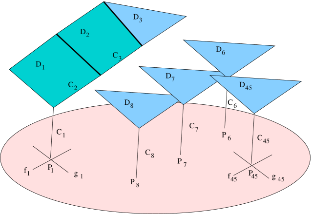
Figure 3: Starting point of our construction of a CY threefold with the desired topology. The curves $f_{i}$ and $g_{i}$ are fibers in the two rulings on $S_{1}$.

Each of the curves and surfaces we have used in this construction can be embedded in a Calabi–Yau neighborhood, and those neighborhoods can be glued together to form a Calabi–Yau neighborhood of the entire structure illustrated in figure 3.

We now pass from this structure to the one we want by a sequence of flops. First, we flop the curves $C_{45}$, $C_{6}$, $C_{7}$, and $C_{8}$, which has the effect of blowing up $S_{1}$ at the four points $P_{45}$, $P_{6}$, $P_{7}$ and $P_{8}$ yielding a del Pezzo surface $S_{5}$. The transformed surfaces $D_{45}$, $D_{6}$, $D_{7}$, $D_{8}$ now meet $S_{5}$ in the flopped curves, as indicated in figure 4.

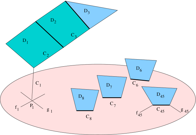
Figure 4: The CY threefold after flopping the curves $C_{45},C_{6},C_{7}$ and $C_{8}$. The curves $f_{45}$, $g_{45}$, $C_{45}$, $C_{6}$, $C_{7}$, and $C_{8}$ are all $(-1)$-curves on $S_{5}$.

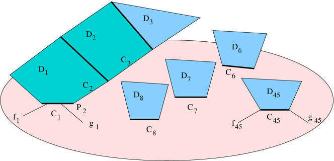
Figure 5: The CY threefold after flopping $C_{1}$. The curves $f_{1}$, $g_{1}$, and $C_{1}$ are additional $(-1)$-curves on $S_{6}$.

Next, we flop the curve $C_{1}$, yielding a del Pezzo $S_{6}$ on which the point $P_{1}$ has been blown up, as indicated in figure 5. The transformed surface $D_{1}$ meets $S_{6}$ in the flopped curve, and the transformed curve $C_{2}$ meets $S_{6}$ in a point $P_{2}$ (“infinitely near” to the first point $P_{1}$). When $C_{2}$ is now flopped, $S_{6}$ is blown up at $P_{2}$ to yield $S_{7}$, as indicated in figure 6. The transformed surface $D_{2}$ meets $S_{7}$ in the most recently flopped curve.

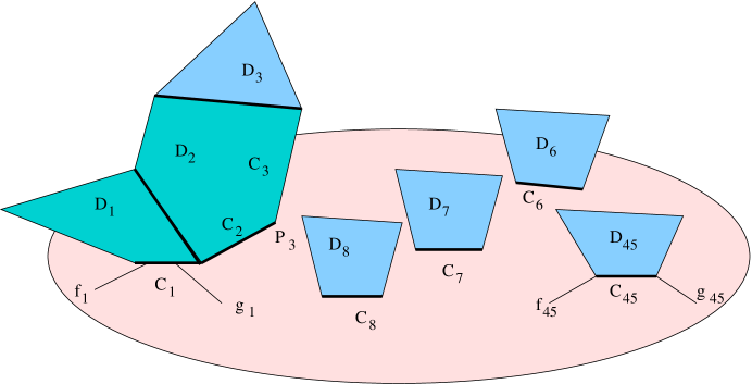
Figure 6: The CY threefold after flopping $C_{2}$. The curve $C_{1}$ has become a $(-2)$-curve, and $C_{2}$ is a $(-1)$-curve on $S_{7}$.

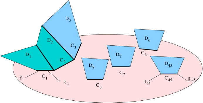
Figure 7: The CY threefold after flopping $C_{3}$. The curves $C_{2}$ has become a $(-2)$-curve, $C_{1}$ remains a $(-2)$-curve, and $C_{3}$ is a $(-1)$-curve on $S_{8}$.

The transformed curve $C_{3}$ meets $S_{7}$ in a point $P_{3}$ (“infinitely near” to $P_{2}$), and when $C_{3}$ is now flopped, $S_{7}$ is blown up at $P_{3}$ to yield $S_{8}$, as indicated in figure 7. (The transformed surface $D_{3}$ meets $S_{8}$ in the most recently flopped curve.) To match the curves on $S_{8}$ to the standard basis for cohomology of a del Pezzo, we set $e_{1}=C_{1}+C_{2}+C_{3}$, $e_{2}=C_{2}+C_{3}$, $e_{3}=C_{3}$, $e_{4}=f_{45}$, $e_{5}=g_{45}$, and $e_{j}=C_{j}$ for $j=6,7,8$ so that $\alpha_{1}=C_{1}$ and $\alpha_{2}=C_{2}$. We can now contract the transforms of $D_{1}$ and $D_{2}$ to a curve of $A_{2}$ singularities, yielding the configuration illustrated in figure 8.

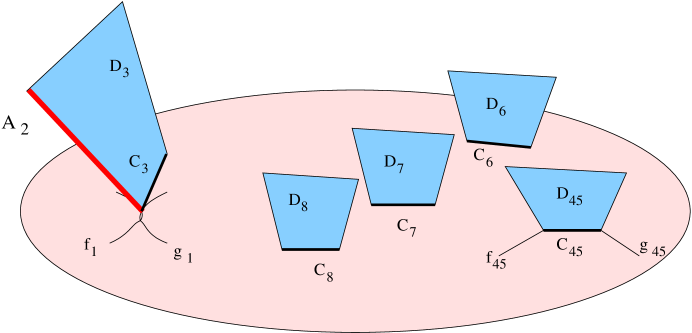
Figure 8: The final configuration: a del Pezzo 8 surface with an $A_{2}$ singularity, embedded into a Calabi–Yau such that two of its exceptional curves are homologous.

To achieve our final desired singular point, we contract the del Pezzo surface $S^{\prime}=S_{8}$ to a point. Let us analyze the properties of this singular point.

First, it is not isolated: there is a curve of $A_{2}$ singularities which eminates from our singular point. This is one of the features we needed, because it allows the fractional branes where were supported on $\alpha_{1}$ and $\alpha_{2}$ to move off of the singular point we are interested in, into the bulk of the Calabi–Yau manifold.

Second, the local Picard group of this singular point has rank $6$: the anticanonical divisor $D_{0}\equiv-K_{S}$ and the transformed divisors $D_{3}$, $D_{45}$, $D_{6}$, $D_{7}$, $D_{8}$ generate a subgroup of the local Picard group of rank six; if there were a seventh generator, the map $\operatorname{Pic}(X)\to\operatorname{Pic}(S)$ would be surjective and the original surface $S_{1}$ would have had the same property, so that its local Picard group would have had rank $2$. But by construction, the surface $S_{1}$ had a local Picard group of rank $1$. We thus have demonstrated the presence of a 3-chain $\Gamma$, with boundary equal to the difference of two exceptional divisors. We can identify this difference with $\alpha_{4}=E_{5}-E_{4}$, which therefore does not exist as a homology class in the full Calabi–Yau.

Thus, via the above geometric procedure, we have succeeded in constructing a compact CY threefold with the properties we need for our D-brane construction. The outlined strategy furthermore preserves the main characteristics of our bottom-up perspective, since it only refers to the local Calabi-Yau neighborhood of the singularity and does not rely on unnecessary assumptions about the full string compactification.

An important physical assumption is that the compact embedding preserves the existence of all constituent fractional branes listed in eqn (56). This is not entirely obvious, since, in particular, the D5 charge around the trivial cycle $\alpha_{4}$ is no longer a conserved quantum number: one could imagine a tunneling process, in which the linear combination (71) of fractional branes combines into a single D5 wrapping $\alpha_{4}$, which subsequently self-annihilates by unwrapping along the 3-chain $\Gamma$. The tunneling process, however, is suppressed because it is non-supersymmetric and the probability can be made exponentially small by ensuring that the 3-volume (measured in units of D-brane tension) of the 3-chain $\Gamma$ is large enough.

6. Conclusion and Outlook

In this paper, we further developed the program advocated in [5], aimed at constructing realistic gauge theories on the world-volume of D-branes at a Calabi–Yau singularity. We have seen that several aspects of the world-volume gauge theory, such as the spectrum of light $U(1)$ vector bosons and the number of freely tunable of couplings, depend on the compact Calabi–Yau embedding of the singularity. In section 3, we have worked out the stringy mechanism by which $U(1)$ gauge symmetries get lifted. As a direct application of this result, we have shown how to construct a supersymmetric Standard Model, however with some extra Higgs fields, on a single D3-brane on a suitably chosen Calabi–Yau threefold with a del Pezzo 8 singularity. The final result for the quiver gauge theory is given in fig 2, where in addition all extra $U(1)$ factors besides hypercharge are massive.

6.1. $U(1)$ Breaking via D-instantons

At low energies, the extra $U(1)$’s are approximate global symmetries, which, if unbroken, would in particular forbid $\mu$-terms. Fortunately, the geometry supports a plethora of D-instantons, that generically will break the $U(1)$ symmetries. Here we make some basic comments on the generic form of the D-instanton contributions.

The simplest type of D-instantons are the euclidean D-branes that wrap compact cycles within the base $X$ of the CY singularity. The ‘basic’ D-instantons of this type are in 1-1 correspondence with the space-time filling fractional branes: they are localized in ${\mathbb{R}}^{4}$, but otherwise have the same Calabi-Yau boundary state and preserve the same supersymmetries as the fractional branes ${\mathsf{F}}_{s}$. Apart from the exponential factor $e^{-{8\pi^{2}/g^{2}_{s}}\;+\,i\,\theta_{s}},$ their contribution is independent of Kähler moduli and can thus be understood at large volume. In this limit, the analysis has essentially already been done in [35, 34, 36]. The result agrees with the expected field theory answer [37], and sensitively depends on $N_{c}-N_{f}$, the number of colors minus the number of flavors for the corresponding node. In our gauge theory we have $N_{f}>N_{c}$, in which case the one-instanton contribution to the superpotential is of the schematic form

$$\delta W={\Omega}(\Phi)\;e^{-8\pi^{2}/g^{2}_{s}\;+\,i\,\theta_{s}}$$ (74)

where $\Omega(\Phi)$ is a chiral multi-fermion operator [37]. The theta angle $\theta_{s}$ in general contains an axion field, that is shifted by the anomalous $U(1)$ gauge rotations. Instanton contributions to the effective action thus generally violate the anomalous $U(1)$ symmetries.

The story for the non-anomalous global $U(1)$ symmetries is analogous. The relevant D-instanton contributions are generated by euclidean D3-branes wrapping the dual 4-cycles $\Sigma_{\alpha}$ within $Y$. The classical D-instanton action reads $S=\mu_{3}{\rm Vol}(\Sigma_{\alpha})-i\!\int_{\Sigma_{\alpha}}\!C_{\it 4}\$ with $\mu_{3}$ the D3-brane tension. Since $\int_{\Sigma_{\alpha}}\!C_{\it 4}=\rho_{\alpha}$ is the Stückelberg field, we observe that the D3-instanton contribution to the superpotential takes the form

$$\quad\delta W={\cal A}(\Phi)\;e^{-\mu_{3}{\rm Vol}(\Sigma_{\alpha})\;+\;i\rho_{\alpha}}\,$$ (75)

Here ${\cal A}(\Phi)$ denotes the perturbative pre-factor, the string analogue of the fluctuation determinant, of the D-instanton. Since the phase factor $e^{i\rho_{\alpha}}$ transforms non-trivially under the corresponding $U(1)$ rotation, the pre-factor must be oppositely charged. After gauge fixing, the value of $\rho_{\alpha}$ will get fixed at by minimizing the potential, and $\rho_{\alpha}$ gets lifted from the low energy spectrum. What remains is a superpotential term that, from the low energy perspective, breaks the global $U(1)$ symmetry.

While we have not yet done the full analysis of these D-instanton effects, it seems reasonable to assume that the desired $\mu$-terms can be generated via this mechanism. Since the D-instanton contribution decreases exponentially with the volume of the 4-cycles $\Sigma_{\alpha}$, it would naturally explain why (some of) the $\mu$-terms are small compared to the string scale.

6.2. Eliminating extra Higgses

Figure 7: An MSSM-like quiver gauge theory, satisfying all rules for world-volume theories in an unoriented string models.

From a phenomenological perspective, the specific model based on the $dP_{8}$ singularity still has several issues that need to be addressed, before it can become fully realistic. Most immediately noticeable is the multitude of Higgs fields, and the fact that supersymmetry is unbroken. Supersymmetry breaking effects may get generated via various mechanisms: via fluxes, nearby anti-branes, non-perturbative string physics, etc. The structure of the SUSY breaking and $\mu$-terms are strongly restricted by phenomenological constraints, such as the suppression of flavor changing neutral currents. However, we see no a priori obstruction to the existence of mechanisms that would sufficiently lift the masses of all extra Higgses and effectively eliminate them from the low energy spectrum.

The presence of the extra Higgs fields is dictated via the requirement (on all D-brane constructions on orientable CY singularities) that each node should have an equal number of in- and out-going lines. To eliminate this feature, it is natural to look for generalizations among gauge theories on orientifolds of CY singularities. Near orientifold planes, D-branes can support real gauge groups like $SO(2N)$ or $Sp(N)$. With this generalization, one can draw a more minimal quiver extension of the SM, with fewer Higgs fields. An example of such a quiver is drawn in fig 7. It should be straightforward to find an orientifolded CY singularity and fractional brane configuration that would reproduce this quiver. The extra $U(1)$ factors in fig 7 can then be dealt with in a similar way as in our $dP_{8}$ example.

Acknowledgments

It is a pleasure to thank Vijay Balasubramanian, David Berenstein, Michael Douglas, Shamit Kachru, Elias Kiritsis, János Kollár, John McGreevy, and Michael Schulz for helpful discussion and comments. This work was supported by the National Science Foundation under grants PHY-0243680 and DMS-0606578 and by an NSF Graduate Research Fellowship (M.B.). D.M.would like to thank the IHES for hospitality and support when part of this work was done. Any opinions, findings, and conclusions or recommendations expressed in this material are those of the authors and do not necessarily reflect the views of the National Science Foundation.

References

- [1] M. R. Douglas and G. W. Moore, “D-branes, Quivers, and ALE Instantons,” hep-th/9603167.
- [2] I. R. Klebanov and E. Witten, “Superconformal field theory on threebranes at a Calabi-Yau singularity,” Nucl. Phys. B 536, 199 (1998) hep-th/9807080.
- [3] D. R. Morrison and M. R. Plesser, “Nonspherical Horizons. 1,” Adv. Theor. Math. Phys. 3, 1 (1999) hep-th/9810201.
- [4] C. Vafa, “The string landscape and the swampland,” arXiv:hep-th/0509212.
- [5] H. Verlinde and M. Wijnholt, “Building the standard model on a D3-brane,” arXiv:hep-th/0508089.
- [6] M. Wijnholt, “Large volume perspective on branes at singularities,” hep-th/0212021.
- [7] C. P. Herzog, “Exceptional collections and del Pezzo gauge theories,” JHEP 0404, 069 (2004), hep-th/0310262.
- [8] A. Bergman and C. Herzog, “The volume of non-spherical horizons and the AdS/CFT correspondence,” arXiv:hep-th/0108020.
- [9] P. S. Aspinwall, “K3 surfaces and string duality,” arXiv:hep-th/9611137.
- [10] C. Vafa and E. Witten, Nucl. Phys. Proc. Suppl. 46, 225 (1996) [arXiv:hep-th/9507050].
- [11] T. W. Grimm and J. Louis, “The effective action of N = 1 Calabi-Yau orientifolds,” Nucl. Phys. B 699, 387 (2004) [arXiv:hep-th/0403067].
- [12] H. Jockers and J. Louis ‘The effective action of D7-branes in Calabi-Yau Orientifolds,’ arXiv:hep-th/0409098.
- [13] Y. K. Cheung and Z. Yin, “Anomalies, branes, and currents,” Nucl. Phys. B 517, 69 (1998) [arXiv:hep-th/9710206].
- [14] M. Marino, R. Minasian, G. W. Moore and A. Strominger, “Nonlinear instantons from supersymmetric p-branes,” JHEP 0001, 005 (2000) [arXiv:hep-th/9911206].
- [15] M. R. Douglas, B. Fiol and C. Romelsberger, JHEP 0509, 006 (2005) [arXiv:hep-th/0002037].
- [16] A. Kapustin and Y. Li, “Stability conditions for topological D-branes: A worldsheet approach,” arXiv:hep-th/0311101.
- [17] K. Intriligator and N. Seiberg, “The runaway quiver,” JHEP 0602, 031 (2006) [arXiv:hep-th/0512347].
- [18] L. E. Ibanez, R. Rabadan and A. M. Uranga, “Anomalous U(1)’s in type I and type IIB D = 4, N = 1 string vacua,” Nucl. Phys. B 542, 112 (1999) hep-th/9808139.
- [19] I. Antoniadis, E. Kiritsis and J. Rizos, “Anomalous U(1)s in type I superstring vacua,” Nucl. Phys. B 637, 92 (2002) [arXiv:hep-th/0204153].
- [20] B. V. Karpov and D. Yu. Nogin, “Three-block Exceptional Collections over del Pezzo Surfaces,” Izv. Ross. Akad. Nauk Ser. Mat. 62 (1998), no. 3, 3–38; translation in Izv. Math. 62 (1998), no. 3, 429–463, alg-geom/9703027.
- [21] D. Berenstein, V. Jejjala and R. G. Leigh, “The standard model on a D-brane,” Phys. Rev. Lett. 88, 071602 (2002) [arXiv:hep-ph/0105042].
- [22] G. Aldazabal, L. E. Ibanez, F. Quevedo and A. M. Uranga, “D-branes at singularities: A bottom-up approach to the string embedding of the standard model,” JHEP 0008, 002 (2000) [arXiv:hep-th/0005067].
- [23] M. Wijnholt, “Parameter space of quiver gauge theories,” arXiv:hep-th/0512122.
- [24] J. Polchinski, “Tensors from K3 orientifolds,” Phys. Rev. D 55 (1997) 6423–6428, hep-th/9606165.
- [25] M. R. Douglas, B. R. Greene, and D. R. Morrison, “Orbifold resolution by D-branes,” Nucl. Phys. B 506 (1997) 84–106, hep-th/9704151.
- [26] D. E. Diaconescu, M. R. Douglas, and J. Gomis, “Fractional branes and wrapped branes,” J. High Energy Phys. 02 (1998) 013, hep-th/9712230.
- [27] A. Lawrence, N. Nekrasov, and C. Vafa, “On conformal field theories in four dimensions,” Nucl. Phys. B 533 (1998) 199–209, hep-th/9803015.
- [28] V. Balasubramanian, P. Berglund, J. P. Conlon and F. Quevedo, “Systematics of moduli stabilisation in Calabi-Yau flux compactifications,” JHEP 0503, 007 (2005) [arXiv:hep-th/0502058].
- [29] D. E. Diaconescu, B. Florea, S. Kachru and P. Svrcek, “Gauge - mediated supersymmetry breaking in string compactifications,” JHEP 0602, 020 (2006) [arXiv:hep-th/0512170].
- [30] Y. Kawamata, “Crepant blowing-up of 3-dimensional canonical singularities and its application to degenerations of surfaces”, Ann. of Math. (2) 127 (1988), 93–163.
- [31] S. Mori,“Threefolds whose canonical bundles are not numerically effective”, Ann. of Math. (2) 116 (1982), 133–176.
- [32] D. R. Morrison and N. Seiberg, “Extremal transitions and five-dimensional supersymmetric field theories”, Nuclear Phys. B 483 (1997), 229–247, arXiv:hep-th/9609070.
- [33] B. R. Greene, D. R. Morrison, and C. Vafa, “A geometric realization of confinement”, Nuclear Phys. B 481 (1996), 513–538, arXiv:hep-th/9608039.
- [34] E. Witten, “Non-Perturbative Superpotentials In String Theory,” Nucl. Phys. B 474, 343 (1996) [arXiv:hep-th/9604030].
- [35] M. Bershadsky, A. Johansen, T. Pantev, V. Sadov and C. Vafa, “F-theory, geometric engineering and N = 1 dualities,” Nucl. Phys. B 505, 153 (1997) [arXiv:hep-th/9612052].
- [36] O. J. Ganor, “A note on zeroes of superpotentials in F-theory,” Nucl. Phys. B 499, 55 (1997) [arXiv:hep-th/9612077].
- [37] C. Beasley and E. Witten, “New instanton effects in supersymmetric QCD,” JHEP 0501, 056 (2005) [arXiv:hep-th/0409149].
- [38] R. Blumenhagen, M. Cvetic and T. Weigand, “Spacetime instanton corrections in 4D string vacua - the seesaw mechanism arXiv:hep-th/0609191.
- [39] L. E. Ibanez and A. M. Uranga, arXiv:hep-th/0609213.
- [40] B. Florea, S. Kachru, J. McGreevy, and N. Saulina, “Stringy instantons and quiver gauge theories” [arXiv:hep-th/0610003].
- [41] D. Berenstein, “Branes vs. GUTS: Challenges for string inspired phenomenology,” arXiv:hep-th/0603103.