Equilibrium configurations of fluids and their stability in higher dimensions

Abstract

We study equilibrium shapes, stability and possible bifurcation diagrams of fluids in higher dimensions, held together by either surface tension or self-gravity. We consider the equilibrium shape and stability problem of self-gravitating spheroids, establishing the formalism to generalize the MacLaurin sequence to higher dimensions. We show that such simple models, of interest on their own, also provide accurate descriptions of their general relativistic relatives with event horizons. The examples worked out here hint at some model-independent dynamics, and thus at some universality: smooth objects seem always to be well described by both “replicas” (either self-gravity or surface tension). As an example, we exhibit an instability afflicting self-gravitating (Newtonian) fluid cylinders. This instability is the exact analogue, within Newtonian gravity, of the Gregory-Laflamme instability in general relativity. Another example considered is a self-gravitating Newtonian torus made of a homogeneous incompressible fluid. We recover the features of the black ring in general relativity.

I Introduction

The shape and stability of liquid drops has been the subject of intense study for more than 200 years, with exciting revivals occurring more or less periodically. In the early days of the topic, the hope was that centimeter-sized drops held together by surface tension could be good models for giant liquid masses held together by self-gravitation. Liquid drops, which could be controlled in the laboratory, should model self-gravitating stars where gravity would replace surface tension. A great deal of what is now known about (rotating) liquid drops is due to the work of J. Plateau plateau who, despite suffering from blindness throughout a good part of his scientific life, conducted many rigorous experimental investigations on the subject (we refer the reader to plateau for details). Starting with a non-rotating drop of spherical shape, Plateau and collaborators progressively increased the rate of rotation (angular velocity, assuming the drop rotates approximately as a rigid body). Plateau found that as the rotation rate increased, the drop progressed through a sequence of shapes which evolved from axisymmetric for slow rotation, to ellipsoidal and two-lobed and finally toroidal at very large rotation. These experimental works have been repeated with basically the same outcome, even in gravity-free environments rotatingdropexperiments (see also rotatingdropexperiments2 ). Theoretical analysis of Plateau’s experiments were started by Poincaré poincaresurfacetension , who proved that there are two very different possible solutions to the equilibrium problem: one is axisymmetric like disks or torii and the other is comprised of asymmetric shapes with two lobes. The analysis was completed by Chandrasekhar chandra , improved upon by Brown and Scriven brownscriven (see also brownscrivenprl ; heine ) and is summarized in Figure 1, taken from brownscriven .

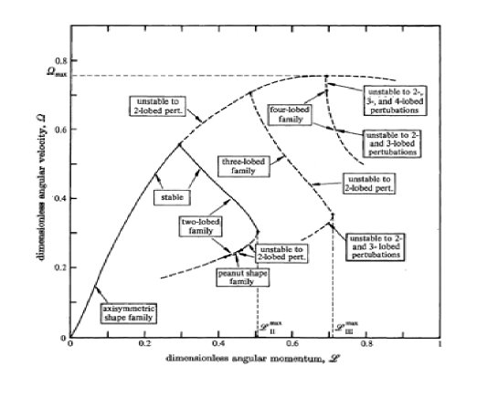
Figure 1: The bifurcation and stability diagram for rotating liquid drops with surface tension (self-gravity is neglected). Shapes are stable along solid branches, unstable along broken ones. The plot depicts dimensionless angular velocity as function of dimensionless angular momentum. The dimensionless angular velocity is $\Omega=\sqrt{\frac{\rho\hat{\Omega}\hat{R}}{8T}}$, where all hatted quantities are dimensionfull, $\hat{R}$ is the radius of a sphere with the same volume as that of the drop, $\rho$ and $T$ are the density and surface tension of the liquid. Likewise, the dimensionless angular momentum J is defined as $J=\hat{J}/4T\hat{R}^{2}\left(8T\hat{R}^{2}\rho\right)$. Although not shown in the plot, the axisymmetric curve bends back to lower angular velocities after it has passed the four-lobed family neutral point. Note also that the maximum allowed angular momentum for stable shapes is denoted by $J_{II}$ in the diagram. Taken from brownscriven .

The Figure shows the (dimensionless, as defined by Brown and Scriven, see caption in Fig. 1) angular velocity as a function of the angular momentum of the drop, and it displays the stability and bifurcation points of the evolution. Let’s focus first on the evolution of axisymmetric figures. Starting from zero angular momentum, where the shape is a spherical surface, one increases the angular momentum. The resulting equilibrium shape evolves from a sphere through oblate shapes to biconcave shapes (see also chandra ). There are no (axisymmetric) equilibrium figures with $\Omega>\Omega_{\rm max}\sim 0.753$. The axisymmetric family does not terminate at $\Omega=\Omega_{\rm max}$, instead it bends back to lower angular velocity, and there are now two axisymmetric figures of equilibrium. The steepest descending branches are torii rotatingdropexperiments2 ; gulliver .

Stability calculations show that all shapes of the axisymmetric family are stable against axisymmetric perturbations, however a real drop is also perturbed by non-axisymmetric modes. The stability calculations show that the drop becomes unstable at $\Omega=\Omega_{II}\sim 0.5599$ brownscriven , where the axisymmetric family is neutrally stable to a two-lobed perturbation. This point marks the bifurcation of a two-lobed family (therefore a non-axisymmetric family). All axisymmetric shapes with $\Omega>\Omega_{II}$ are unstable against two-lobed perturbations, but there are additional points of neutral stability, which are also bifurcation points: the three- and four-lobed perturbations are shown in the diagram 1 but there are others heine . The first, most important non-axisymmetric surface, the two-lobed family, branches off at $\Omega=\Omega_{II}$, and is initially (near the bifurcation point) stable. In Figure 2 we show some typical members of that sequence (see phdheine , where this figure was taken from, for further details).

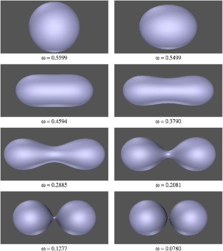
Figure 2: This plot shows a sequence of members of the two-lobed family of drop shapes for several values of angular velocity. The two-lobed drops seem to approach a limiting surface consisting of two spheres touching each other in one point as $\Omega$ approaches 0. The first shape, with $\Omega=0.5599$, corresponds to the first (two-lobed) bifurcation point in Fig. 1. For $\Omega=0.2885$ for instance, the figure is peanut shaped, and we can situate the corresponding family in Fig. 1. Taken from phdheine .

It turns out that the evolution of self-gravitating fluids, i.e., stars, follows a very similar diagram, as shown in Figure 3. Finding the equilibrium configurations of self-gravitating rotating homogeneous fluids is an extremely important problem, which has met intense activity ever since the first discussions by Newton and others (see history and also the excellent and concise introduction in chandrabookellipsoidal ), which was revisited some 50 years ago by Chandrasekhar and co-workers chandrabookellipsoidal . In three spatial dimensions, the most basic figures of equilibrium of rotating bodies are the MacLaurin and Jacobian sequences . The MacLaurin sequence is a sequence of oblate spheroids along which the eccentricity of meridional sections increases from zero to one. Jacobi showed that for each value of $\Omega^{2}$, the square of the angular velocity of rotation, there are actually two permissible figures of equilibrium. The other is a tri-axial ellipsoid, belonging to the Jacobi sequence, which branches off from the MacLaurin sequence. This is the first of several points of bifurcation which distinguish the permissible sequences of figures of equilibrium of uniformly rotating homogeneous masses. If one starts from a non-rotating homogeneous fluid ellipsoid in the MacLaurin sequence and increases the angular momentum of the body, one will first come across the Jacobi branch, where the ellipsoid becomes unstable with regard to the first non-axisymmetric perturbation chandrabookellipsoidal (which are the self-gravitating analogues of the shapes in Figure 2). Continuing, still along the MacLaurin sequence and increasing angular momentum, one next comes to the bifurcation point of other non-axisymmetric figures: the “triangle”, the “square” and “ammonite” sequences chandrabookellipsoidal ; eriguchi . One finally encounters the first axisymmetric sequence. The bodies of this sequence pinch together at the centre and eventually form Dyson’s anchor-rings, or torus-like configuration dyson ; bardeen ; wong ; eriguchisugimoto ; ansorg . It is apparent that the bifurcation diagram for self-gravitating fluids, Figure 3 is very similar to the one for non-gravitating fluids with surface tension, shown in Figure 1. Thus, whenever the treatment of self-gravitation proves too difficult, the surface tension model is a good guide.

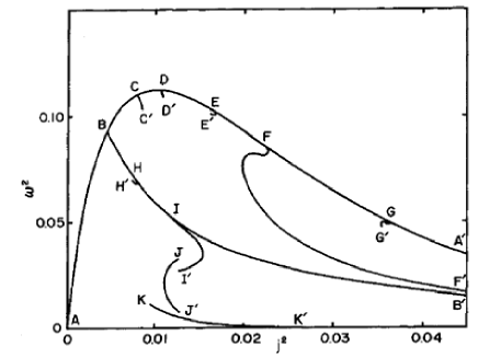
Figure 3: The bifurcation diagram for rotating self-gravitating, incompressible homogeneous stars. Here we show the angular velocity as function of the angular momentum for several possible families. The data and notation are those of Eriguchi and Hachisu eriguchi . The line $A-A^{\prime}$ is the MacLaurin sequence, $B-B^{\prime}$ the Jacobi sequence, $C-C^{\prime}$ triangle sequence, $D-D^{\prime}$ the square sequence, $E-E^{\prime}$ ammonite sequence, $F-F^{\prime}$ the one-ring sequence, $G-G^{\prime}$ the two-ring sequence, $H-H^{\prime}$ the pear-shaped sequence, $I-I^{\prime}$ the dumb-bell sequence, $J-J^{\prime}$ the Darwin sequence and finally $K-K^{\prime}$ is the two point-mass sequence. Note the similarities with Fig. 1. See eriguchi for further details.

A realistic star is neither homogeneous nor incompressible and it certainly isn’t held together by surface tension. However, it seems logical to build our understanding using simpler models. We have gone a long way with simpler related models: another well-known example, where the fluid drop model proved extremely useful, is Bohr and Wheeler’s bohrwheeler proposal to describe nuclear fission as the rupture of a rotating charged liquid drop, where now the surface tension plays the role of nuclear forces. A review with a detailed and unified discussion of charged nuclei, astronomical bodies and fluid drops can be found in swiatecki (a concise and complete account of the history of this subject, along with some good quality figures can be also found in phdheine ). Liquid drops can model self-gravitating systems. Can they model extremely compact, highly relativistic objects like black holes? The answer, quite surprisingly, seems to be yes cardosodiasglrp . Regarding the event horizon as a kind of fluid membrane is a position adopted in the past membraneparadigm . A simple way to see that this is a natural viewpoint, is to take the first law of black hole mechanics BardCartHawk which describes how a black hole (we will take for simplicity uncharged, static objects), characterized by a mass $M$, horizon area $A$, and temperature $T=1/(32\pi M)$, evolves when we throw an infinitesimal amount of matter into it:

$$dM=TdA\,.$$ (1)

We now know that the correct interpretation of this law is that black holes radiate, and therefore can be assigned a temperature bekenstein ; hawking . The second law of black hole mechanics $dA\geq 0$ is then just the second law of thermodynamics. But we can also argue that Equation (1) can be looked at as a law for fluids, with $T$ being an effective surface tension booktension . The first works in black hole mechanics actually considered $T$ as a surface tension (see the work by Smarr smarr and references therein), which is rather intuitive: the potential energy for fluids, associated with the storage of energy at the surface, is indeed proportional to the area. Later, Thorne and co-workers membraneparadigm developed the “membrane paradigm” for black holes, envisioning the event horizon as a kind of membrane with well-defined mechanical, electrical and magnetic properties. Not only is this a simple picture of a black hole, it is also useful for calculations and understanding what black holes are really like. This analogy was put on a firmer ground by Parikh and Wilczek wilczek , who provided an action formulation of this membrane picture. There are other instances where a membrane behavior seems evident: Eardley and Giddings eardley , studying high-energy black hole collisions found a soap bubble-like law for the process, while many modern interpretations of black hole entropy and gravity “freeze” the degrees of freedom in a lower dimensional space, in what is known as holography holo . In kovtun1 it was shown that a “membrane” approach works surprisingly well, yielding precisely the same results as the AdS/CFT correspondence. There have also been attempts to work the other way around: computing liquid surface tension from the (analog) black hole entropy surfacetbh . As a last example of a successful use of the membrane picture, Cardoso and Dias cardosodiasglrp have recently been able to mimic many of the aspects of a gravitational instability by using a simple fluid analogy. We will comment on this work later on.

Having said this, it strikes one as very odd that the study of simple fluid models has not been extended to higher dimensions. Extra dimensions, besides the four usual ones, seem to be needed for consistency in all or many of candidate theories of unification. We have in mind not only string theory zwie where the extra dimensions are compactified to a very small scale, but also recent theories with large add or warped extra dimensions rs . Therefore, an understanding of higher dimensional gravitating objects is imperative. However, even though there are several known exact solutions to Einstein equations in more than four dimensions describing black objects (with event horizons), nothing or very little is known about the simpler Newtonian fluid equilibrium configurations, with or without self-gravity.

For instance, higher dimensional black hole solutions with spherical topology have long been known tangherlini ; myersperry , which generalize the four-dimensional Kerr-solution to higher dimensions. In four spacetime dimensions one can show that the topology of a black hole must be a sphere, but that’s no longer the case in higher dimensions. A simple example is to consider extra flat dimensions, for instance ${\rm Schwarzschild}\times R$, which is still a solution to the vacuum Einstein equations. These extended solutions can then have different topologies, like a cylinder, and are called back strings horowitzstrominger . Yet another example is the five-dimensional black ring Emparan:2001wn ; Elvang:2003mj , having the topology of a torus.

It is curious to note that we are in possession of several exact solutions to the full Einstein equations and yet nothing is known about the simpler case of self-gravitating Newtonian fluids or even fluids without gravity but with surface tension. To be specific, we found a solution as “strange” as a black ring in five dimensions, yet we do not know how a rotating, self-gravitating Newtonian fluid behaves as a function of the rotation rate, for higher dimensional spacetimes. These simpler objects should be much easier to study, while carrying precious information about their more compact cousins with event horizons. There are several topics that could and should be addressed within this research line:

(i) Do the fluid equations admit toroidal-like configurations, which may collapse to black rings for very high densities? Are these stable?

(ii) Ultra-spinning black holes in spacetime dimensions larger than four are conjectured to be unstable emparanmyers ; cardosodiasglrp for large enough rotation rates. If the four-dimensional results for self-gravitating fluids or for fluids with surface tension carry over, this is to be expected. As we saw in the evolution diagrams, axisymmetric configurations are unstable for rotation rates larger than a given threshold, decaying to a two-lobe, asymmetric configuration. This suggests that the end-state of ultra-spinning black holes is a two lobe, asymmetric state like those in Figure 2. This possibility was already put forward in emparanmyers , but the arguments presented here make this a much stronger possibility. These shapes would then presumably spin-down due to radiation emission. Can we use simple fluids with surface tension or with self-gravity to model this process? Can we estimate the rotation rate at which instability occurs?

(iii) The black strings and p-branes are unstable against a gravitational sector of perturbations. Can we simulate this instability with fluids? A first step was taken in cardosodiasglrp , where it was shown that a simple fluid with surface tension can account for most of the properties of this instability. Can we add self-gravity to the model? Can we include rotational and charge effects?

(iv) Can we build the evolution and bifurcation diagrams for fluids with surface tension (or with self-gravity) in higher dimensions? Can we deduce other solutions to the general relativistic equations using these simpler models? Can we infer other properties of already known solutions?

These are just some of the topics that could be addressed with simple Newtonian fluid models, but the list could easily be made much longer. The goal of the present work is to pave the way to some of these possible developments, but especially to show that these simple models do yield relevant information. We will attack the problem in its two versions: fluids held together by surface tension and by self-gravity.

Plan of the paper

This paper is divided in two parts, Part I in which we deal with fluids held by surface tension and Part II where we deal with fluids held together by self-gravity.

We start with Section II, where we review the meaning of angular momentum in higher dimensions and also the symmetries of a rotating body. We also specify the two most important cases (case I and II) we shall deal with throughout the paper. In Section III we lay down the basic equations of hydrostatics and hydrodynamics in higher dimensions and in Section IV we write the formalism necessary to analyse small deviations for equilibrium. The formalism just laid down is then used in the next sections. In Section V we study the equilibrium figure of rotating drops. Oscillation modes of non-rotating spherical drops are derived in Appendix A and constitutes a generalization to arbitrary number of dimensions of the well-known result in three spatial dimensions. In Section VI we discuss equilibrium torus-like configurations of rotating fluids held together by surface tension, and show that these share common features with their vacuum general-relativistic counterpart, the black rings. In Section VII we study the stability of the equilibrium figures discussed in Section A against small perturbations. We compute neutral modes of oscillation and the onset of instability which allows one to derive the bifurcation diagram for the case of one non-vanishing angular momentum. We finish this part with Section VIII by reviewing the Rayleigh-Plateau instability of a thin long cylinder in higher dimensions cardosodiasglrp , which could be a good model for the Gregory-Laflamme instability. We discuss possible effects of rotation and magnetic fields.

In the second part we deal with self-gravitating fluids in higher dimensions. We start in Section IX by considering an infinite cylinder of self-gravitating homogeneous fluid. We show that this cylinder is unstable against a classical instability, here termed Dyson-Chandrasekhar-Fermi (DCF) instability, which we demonstrate to be the exact analogue of the Gregory-Laflamme gl instability of black strings. We discuss implications of this result for rotating and charged fluids and black strings. We then discuss in Section X toroidal equilibrium configurations of self-gravitating fluid (often termed Dyson rings) and we compare them to exact general relativistic toroidal-like configurations, the black ring solution. Finally, in Section XI we write down the basic equations that generalize the MacLaurin and Jacobi sequence to higher dimensions, equations which could be used in future numerical work to reconstruct the whole bifurcation diagram. Oscillation modes of non-rotating globes are derived in Appendix B and constitute a generalization to arbitrary number of dimensions of the well-known result by Kelvin in three spatial dimensions. We close in Section XII with a discussion of the results, implications and suggestions for future work.

This work is by no means complete. Many important topics are left for future work, we discuss some of these in the concluding remarks.

Notation

There are many different symbols used throughout the text. For clarity we find it useful to make a short list of the most often used symbols.

• $D\rightarrow$ total number of spatial dimensions.

• $x^{i}=(x^{a},x^{A})\rightarrow$ coordinates of a rotating body. We consider two particular cases: in case I there is a single rotation plane, and $a=1,2$; $A=3,...,D$; in case II, $D$ is odd and there are $\frac{D-1}{2}$ rotation planes. In this case $a=1,...D-1$; $A=D$.

• $C_{D}\rightarrow$ the area of the unit $(D-1)$-sphere, $C_{D}=\frac{2\pi^{D/2}}{\Gamma\left(\frac{D}{2}\right)}$.

• $\varpi\rightarrow$ radial coordinate in cylindrical coordinates.

• $\omega\rightarrow$ Fourier transform variable. The time dependence of any field is written as $e^{\omega t}$. In the case of a stable oscillation, it is related to the frequency by $\omega^{2}=-\sigma^{2}$. Note that pure imaginary values of $\omega$ mean a stable oscillation.

• $\Omega\rightarrow$ angular velocity.

• ${\cal B}({\bf x})\rightarrow$ Gravitational potential.

• $G\rightarrow$ Newton’s constant in $D-$dimensions, defined by writing the gravitational potential as

  $${\cal B}({\bf x})\equiv G\int_{V}\frac{\rho(\vec{x}^{\prime})}{|\vec{x}-\vec{x}^{\prime}|^{D-2}}d^{D}x^{\prime}\,.$$ (2)

  This is perhaps not the most common definition. A popular definition of Newton’s constant is the one adopted by Myers and Perry myersperry and the relation between the two is derived in Appendix E.

• $T\rightarrow$ magnitude of surface tension, defined by $P=Tn^{i}_{,i}$ where $P$ is the pressure in the interior of the body (we take the exterior pressure to be zero). We take ${\bf n}$ to be the outward normal to the surface the body.

• $P\rightarrow$ Pressure.

• $V\rightarrow$ Volume.

• $\rho\rightarrow$ density.

• $\lambda\rightarrow$ wavelength of a given perturbation.

• $k\rightarrow$ wavenumber $\equiv 2\pi/\lambda$.

• $I^{ij}\equiv\int_{V}\rho x^{i}x^{j}d^{D}x\rightarrow$ Moment of inertia.

Part I Fluids held by surface tension

II Symmetries and geometrical description of a multi-dimensional rotating body

Let us consider a stationary rotating object in $D$-dimensional Euclidean space, with coordinates $x^{i}=(x^{1},\dots,x^{D})$. The rotation group in $D$ dimensions, $SO(D)$, has $D(D-1)/2$ generators $J^{ij}=J^{[ij]}$. Each generator $J^{ij}$ corresponds to an $SO(2)$ rotation, on the plane $x^{i}-x^{j}$.

In a suitable coordinate frame $J=(J^{ij})$ can be brought to the standard form (see for instance myersperry )

$$J=\left(\begin{array}[]{ccc}\begin{array}[]{cc}0&J_{1}\\ -J_{1}&0\\ \end{array}&&\\ &\begin{array}[]{cc}0&J_{2}\\ -J_{2}&0\\ \end{array}&\\ &&\ddots\\ \end{array}\right)\,.$$ (3)

This means that in this frame the rotation is a composition of a rotation in the plane $x^{1}-x^{2}$, a rotation in the plane $x^{3}-x^{4}$, and so on, without mixings. The rotation is then characterized by $[D/2]$ generators (where $[\cdot]$ denotes the integer part), which are the generators of the Cartan subalgebra of $SO(D)$ (namely, the maximal abelian subalgebra of $SO(D)$). In other words, in $D$ dimensions there are

$${\cal N}=\left[\frac{D}{2}\right]$$ (4)

independent angular momenta.

We will consider two particular cases:

• Only one angular momentum is non-vanishing: $J_{1}\neq 0$, $J_{i>1}=0$.

• All angular momenta are non-vanishing, and they are equal: $J_{1}=J_{2}=\dots=J_{\cal N}$; in this case we also assume $D$ to be odd.

These will be referred to as case I and II respectively throughout the whole article.

II.1 Case I. One non-vanishing angular momentum

In this case we are selecting a one-dimensional rotation subgroup

$$SO(2)\subset SO(D)\,.$$ (5)

This means selecting a single rotation plane, $x^{1}\!-\!x^{2}$. We assume our object has the maximal symmetry compatible with this rotation:

$$G=SO(2)\times SO(D-2)\subset SO(D)\,.$$ (6)

If we decompose the coordinates under $G$ as

$$x^{i}=(x^{a},x^{A});~{}~{}~{}~{}a=1,2;~{}A=3,\dots,D\,,$$ (7)

and we define

$$\varpi \equiv \sqrt{(x^{1})^{2}+(x^{2})^{2}}\,,$$

$$z \equiv \sqrt{(x^{3})^{2}+\dots+(x^{D})^{2}}\,,$$ (8)

the surface of our object depends only on $\varpi$ and $z$, and its equation can be written as

$$z=f(\varpi)\,.$$ (9)

i.e.

$$\Xi\equiv z-f(\varpi)=0\,,$$ (10)

therefore the surface does not depend on the angle in the $x^{1}\!-\!x^{2}$ plane, and it does not depend on the $D-3$ angles among $x^{3},\dots,x^{D}$. We also define

$$\phi\equiv\frac{df}{d\varpi}\,.$$ (11)

Notice that it must be $\phi=-\infty$ when $z=0$ for the surface to be smooth.

Being $\varpi_{,a}=\frac{x^{a}}{\varpi}$, the normal to the surface is

$$\Sigma_{,i}=(\Sigma_{,a},\Sigma_{,A})=\left(-\phi\frac{x^{a}}{\varpi},\frac{x^{A}}{z}\right)$$ (12)

with modulus $\delta^{ij}\Sigma_{,i}\Sigma_{,j}=1+\phi^{2}$, so the normal unit vector is

$$n^{i}=\left(-\phi\frac{x^{a}}{\varpi\sqrt{1+\phi^{2}}},\frac{x^{A}}{z\sqrt{1+\phi^{2}}}\right)\,.$$ (13)

Since the pressure is related to surface tension via $P=Tn^{i}_{,i}$, we will need a general relation to compute $n^{i}_{,i}$. Let us then compute $n^{i}_{,i}=n^{a}_{,a}+n^{A}_{,A}$ for this case I. We have

$$n^{a}_{,a} = -\frac{\phi^{\prime}}{(1+\phi^{2})^{3/2}}-\frac{\phi}{\varpi\sqrt{1+\phi^{2}}}=-\frac{1}{\varpi}\frac{d}{d\varpi}\frac{\varpi\phi}{\sqrt{1+\phi^{2}}}$$

$$n^{A}_{,A} = \frac{1}{\sqrt{1+\phi^{2}}}\frac{D-3}{z}\,.$$ (14)

II.2 Case II. All angular momenta coincident, and $D$ odd.

In this case the rotation group is broken to its Cartan subalgebra

$$(SO(2))^{\frac{D-1}{2}}\subset SO(D)\,.$$ (15)

The rotation planes are

$$x^{1}-x^{2},~{}x^{3}-x^{4},~{}\dots,~{}x^{D-2}-x^{D-1}\,,$$ (16)

and the $x^{D}$ axis is left unchanged by the rotation. The decomposition of the coordinates is now

$$x^{i}=(x^{a},x^{A});~{}~{}~{}a=1,\dots,D-1\,;~{}~{}~{}A=D\,.$$ (17)

We define

$$\varpi \equiv \sqrt{(x^{1})^{2}+(x^{2})^{2}+\dots+(x^{D-1})^{2}}\,,$$

$$z \equiv x^{D}\,.$$ (18)

The surface does not depend on the $D-2$ angles among the $x^{a}$. We also define

$$\phi\equiv\frac{df}{d\varpi}\,.$$ (19)

Notice that it must be $\phi=-\infty$ when $z=0$ for the surface to be smooth.

Being $\varpi_{,a}=\frac{x^{a}}{\varpi}$, the normal to the surface is

$$\Sigma_{,i}=\left(-\phi\frac{x^{a}}{\varpi},0\right)\,,$$ (20)

with modulus $\delta^{ij}\Sigma_{,i}\Sigma_{,j}=1+\phi^{2}$, so the normal unit vector is

$$n^{i}=\left(-\phi\frac{x^{a}}{\varpi\sqrt{1+\phi^{2}}},0\right)\,.$$ (21)

Finally,

$$n^{i}_{,i} = n^{a}_{,a}=-\frac{1}{\varpi^{D-2}}\frac{d}{d\varpi}\left(\frac{\varpi^{D-2}\phi}{\sqrt{1+\phi^{2}}}\right)\,.$$ (22)

III Hydrodynamical and hydrostatical equations

Let ${\bf X}=(X^{i})$ the position vector of a fluid element in the inertial frame, and ${\bf x}=(x^{i})$ its position vector in the rotating frame, i.e.

$${\bf X}=R{\bf x}$$ (23)

where $R=R_{I}$ or $R_{II}$ according to the case under consideration and

$$R_{I}=\left(\begin{array}[]{cc|ccc}\cos\Omega t&\sin\Omega t&&&\\ -\sin\Omega t&\cos\Omega t&&&\\ \hline\cr&&1&&\\ &&&\dots&\\ &&&&1\\ \end{array}\right)\,;~{}~{}~{}~{}~{}~{}~{}~{}R_{II}=\left(\begin{array}[]{cccc}\begin{array}[]{cc}\cos\Omega t&\sin\Omega t\\ -\sin\Omega t&\cos\Omega t\\ \end{array}&&&\\ &\ddots&\\ &&\begin{array}[]{cc}\cos\Omega t&\sin\Omega t\\ -\sin\Omega t&\cos\Omega t\\ \end{array}&\\ &&&1\\ \end{array}\right)$$ (24)

are $D$-dimensional rotation matrices in the cases I, II respectively. We introduce the velocity ${\bf\cal V}$ and acceleration ${\bf\cal A}$ by

$$\dot{\bf X} = R{\bf\cal V}$$

$$\ddot{\bf X} = R{\bf\cal A}$$ (25)

where an overdot denotes time differentiation.

The hydrodynamical equation, in the inertial frame, is

$$\ddot{X}^{i}=-\frac{1}{\rho}\frac{\partial P}{\partial X^{i}}$$ (26)

(with $P$ pressure and $\rho$ constant density of the fluid) which, applying $R^{-1}$, gives

$${\cal A}^{i}=-\frac{1}{\rho}\frac{\partial}{\partial x^{i}}P\,.$$ (27)

Let us compute ${\bf\cal A}$. We have

$${\bf\cal V}=R^{T}\dot{R}{\bf x}+\dot{\bf x}$$ (28)

and then

$${\bf\cal A}=R^{T}\dot{R}{\bf\cal V}+\dot{\bf\cal V}=(R^{T}\dot{R})^{2}{\bf x}+2R^{T}\dot{R}\dot{\bf x}+\ddot{\bf x}\,.$$ (29)

We have that the only non-vanishing components of $R^{T}\dot{R}$ are

$$(R^{T}\dot{R})^{ab}=-\Omega\epsilon^{ab}$$ (30)

where $\epsilon^{ab}=\epsilon^{[ab]}$, and $\epsilon^{12}=1$ in the case I, $\epsilon^{12}=\epsilon^{34}=\dots=\epsilon^{(D-2)(D-1)}=1$ in the case II.

Therefore, in both cases $((R^{T}\dot{R})^{2})^{ab}=\Omega^{2}\delta^{ab}$, and

$$\ddot{x}^{a} = -\frac{1}{\rho}\frac{\partial P}{\partial x^{a}}+\Omega^{2}x^{a}+2\Omega\epsilon^{ab}\dot{x}^{b}$$ (31)

$$\ddot{x}^{A} = -\frac{1}{\rho}\frac{\partial P}{\partial x^{A}}\,.$$ (32)

The second term in the right hand side of (31) is the centrifugal force and the third term is the generalized Coriolis force. At equilibrium $\dot{x}^{i}=\ddot{x}^{i}=0$, therefore

$$\frac{\partial P}{\partial x^{a}} = \rho\Omega^{2}x^{a}\,,$$

$$\frac{\partial P}{\partial x^{A}} = 0\,.$$ (33)

thus

$$P=P_{0}+\frac{1}{2}\rho\Omega^{2}\varpi^{2}\,.$$ (34)

This formula is valid both in case I and in case II, i.e., when there is one non-vanishing angular momentum and when all of them coincide (and $D$ is odd).

IV The virial theorem, surface-energy tensor and small perturbations

We would ultimately wish to assess stability of rotating drops, in order to generalize Fig. 1 to higher dimensions. This calculation would also provide some hints as to whether or not one should expect to see instabilities in black objects in higher dimensions, as we stressed in the Introduction. To attack this problem we will follow Chandrasekhar’s chandra approach, to which we refer for further details. Alternative (numerical) approaches, perhaps more complete but more complex also, are described by Brown and Scriven brownscriven and also Heine heine .

IV.1 The virial theorem in the inertial frame

Consider a fluid of volume $V$ with uniform density $\rho$, bounded by a surface $S$. The external pressure, for simplicity, is taken to be zero. Due to the existence of surface tension, the pressure $P$ immediately adjacent to $S$, on the interior, is given in terms of the surface tension magnitude $T$ by

$$P=Tn^{i}_{,i}\,.$$ (35)

Multiplying (26) by $X^{j}$ and integrating over the volume $V$ of the fluid we get

$$\frac{d}{dt}\int_{V}\rho\dot{X}^{i}X^{j}d^{D}X=2{\cal I}^{ij}-\int_{V}X^{j}\frac{\partial P}{\partial X^{i}}d^{D}X\,,$$ (36)

where ${\cal I}^{ij}=\frac{1}{2}\int_{V}\rho\dot{X}^{i}\dot{X}^{j}d^{D}X$ is the inertia tensor. Integrating by parts the second term on the R.H.S. of (36) we have

$$\int_{V}X^{j}\frac{\partial P}{\partial X^{i}}d^{D}X=\int_{S}X^{j}PdS^{i}-\delta^{ij}\int_{V}Pd^{D}X\,,$$ (37)

where $dS^{i}=n^{i}dS$ and $dS$ is the $(D-1)$-dimensional surface element on $S$. Using (35) we further have

$$\int_{V}X^{j}\frac{\partial P}{\partial X^{i}}d^{D}X=T\int_{S}X^{j}n^{i}_{,i}dS^{i}-\delta^{ij}\int_{V}Pd^{D}X\,.$$ (38)

Introducing this result in (36) one gets the virial theorem

$$\frac{d}{dt}\int_{V}\rho\dot{X}^{i}X^{j}d^{D}X=2{\cal I}^{ij}+{\mathfrak{S}}^{ij}+\delta^{ij}\Pi\,,$$ (39)

where

$$\Pi = \int_{V}Pd^{D}X\,,$$ (40)

$${\mathfrak{S}}^{ij} = -T\int_{S}X^{j}n^{k}_{,k}dS^{i}\,.$$ (41)

The quantity ${\mathfrak{S}}^{ij}$ is the surface-energy tensor chandra . Conservation of angular momentum guarantees that $\mathfrak{S}^{ij}$ is symmetric. Indeed,

$$\frac{d}{dt}\int_{V}\rho(\dot{X}^{i}X^{j}-\dot{X}^{j}X^{i})d^{D}X=\mathfrak{S}^{ij}-\mathfrak{S}^{ji}=0\,.$$ (42)

IV.2 The virial theorem in the rotating frame

In a rotating frame of reference the equations of motion are written down in (32). Multiplying those equations by $x^{j}$, integrating over $V$ and using the previous sequence of transformations we get

$$\frac{d}{dt}\int_{V}\rho\dot{x}^{a}x^{j}d^{D}x = 2{\cal I}^{aj}+{\mathfrak{S}}^{aj}+\delta^{aj}\Pi+\Omega^{2}I^{aj}+2\Omega\epsilon^{ac}\int_{V}\rho\dot{x}^{c}x^{j}d^{D}x\,,$$ (43)

$$\frac{d}{dt}\int_{V}\rho\dot{x}^{A}x^{j}d^{D}x = 2{\cal I}^{Aj}+{\mathfrak{S}}^{Aj}+\delta^{Aj}\Pi\,,$$ (44)

where

$$I^{aj}=\int_{V}\rho x^{a}x^{j}d^{D}x\,.$$ (45)

The tensor $\mathfrak{S}^{ij}$ is symmetric in the rotating frame, too, as can be shown by transforming it with the rotation matrix $R$.

We remind the reader that according to our conventions the indices $i,j$ can take any values between $1$ and $D$, but the indices $a,\,b$ and $A,\,B$ are restricted according to the situation we consider (case I or II), described in Equations (7) and (17). In the following we always consider the rotating reference frame.

IV.3 Virial equations for small perturbations

Having solved for the equilibrium equations and found the shape for a given rotating drop (this problem will be explicitly worked out in the next Section V), we ask whether this is a stable equilibrium configuration or not. To answer this we follow the usual procedure to assess stability: we perturb the equilibrium configuration. Suppose then that a drop in a state of equilibrium is slightly disturbed. All background quantities $Q_{0}$ are then changed by an amount $\delta Q_{0}$. The motions are described by a Lagrangian displacement of the form

$${\bf\xi}(x)e^{\omega t}\,,$$ (46)

where $\omega$ is to be determined from the problem. In the case of constant density, $\xi$ is divergence free. Define

$$\Gamma^{i;j}=\int_{V}\rho\xi^{i}x^{j}d^{D}x\,,$$ (47)

where the semi-colon indicates that a moment with respect to coordinate space is being evaluated. Define also

$$\Gamma^{ij}\equiv\Gamma^{i;j}+\Gamma^{j;i}\,.$$ (48)

Then the perturbation equations read chandra

$$\omega^{2}\Gamma^{a;j}-2\omega\Omega\epsilon^{ac}\Gamma^{c;j} = \delta{\mathfrak{S}}^{aj}+\Omega^{2}\Gamma^{aj}+\delta^{aj}\delta\Pi\,,$$ (49)

$$\omega^{2}\Gamma^{A;j} = \delta{\mathfrak{S}}^{Aj}+\delta^{Aj}\delta\Pi\,.$$ (50)

The surface integrals $\delta\mathfrak{S}^{ij}$ have the form

$$\delta\mathfrak{S}^{ij} = -T\delta\int_{S}x^{j}n^{k}_{~{},k}dS^{i}=-T\left[\int_{S}\xi^{j}n^{k}_{~{},k}dS^{i}+\int_{S}x^{j}\delta(n^{k}_{~{},k})dS^{i}+\int_{S}x^{j}n^{k}_{~{},k}\delta(dS^{i})\right]$$ (51)

$$= -T\left[\int_{S}\xi^{j}n^{k}_{~{},k}dS^{i}+\int_{S}x^{j}\delta(n^{k}_{~{},k})dS^{i}-\int_{S}x^{j}n^{k}_{~{},k}\frac{\partial\xi^{l}}{\partial x^{i}}dS^{l}\right]$$

where we have used the general result (see for instance chandra )

$$\delta(dS^{i})=\xi^{j}_{~{},j}dS^{i}-\frac{\partial\xi^{j}}{\partial x^{i}}dS^{j}$$ (53)

and $\xi^{j}_{~{},j}=0$. Furthermore, we have (see chandra )

$$\delta(n^{i}_{~{},i})=(\delta n^{i})_{~{},i}-\frac{\partial n^{i}}{\partial x^{k}}\frac{\partial\xi^{k}}{\partial x^{i}}$$

$$\delta n^{i}=\left(n^{k}n^{l}\frac{\partial\xi^{k}}{\partial x^{l}}\right)n^{i}-n^{j}\frac{\partial\xi^{j}}{\partial x^{i}}\,.$$ (54)

Equations (49), (50) can be decomposed as

$$\omega^{2}\Gamma^{a;b}-2\omega\Omega\epsilon^{ac}\Gamma^{c;b} = \delta{\mathfrak{S}}^{ab}+\Omega^{2}\Gamma^{ab}+\delta^{ab}\delta\Pi\,,$$ (55)

$$\omega^{2}\Gamma^{A;B} = \delta{\mathfrak{S}}^{AB}+\delta^{AB}\delta\Pi\,,$$ (56)

$$\omega^{2}\Gamma^{a;A}-2\omega\Omega\epsilon^{ac}\Gamma^{c;A} = \delta{\mathfrak{S}}^{aA}+\Omega^{2}\Gamma^{aA}\,,$$ (57)

$$\omega^{2}\Gamma^{A;a} = \delta{\mathfrak{S}}^{Aa}\,.$$ (58)

These are the basic equations we will use later on to perform a stability analysis of rotating drops in higher dimensions. To complete the calculations we first need to compute the equilibrium figures of rotating drops and we this in the following.

V Equilibrium shape of a rotating drop

V.1 Case I. One non-vanishing angular momentum

From equations (14), (34), (35) we find

$$P_{0}+\frac{1}{2}\rho\Omega^{2}\varpi^{2}=T\left(-\frac{1}{\varpi}\frac{d}{d\varpi}\frac{\varpi\phi}{\sqrt{1+\phi^{2}}}+\frac{1}{\sqrt{1+\phi^{2}}}\frac{D-3}{z}\right)\,,$$ (59)

thus

$$\frac{1}{2}P_{0}\varpi^{2}+\frac{1}{8}\rho\Omega^{2}\varpi^{4}=-T\frac{\varpi\phi}{\sqrt{1+\phi^{2}}}+(D-3)TI+C$$ (60)

where $C$ is a constant, and $I$ is the integral

$$I(\varpi)=\int_{0}^{\varpi}{\frac{d\varpi^{\prime}\varpi^{\prime}}{f(\varpi^{\prime})\sqrt{1+\left(\frac{df}{d\varpi^{\prime}}\right)^{2}}}}\,.$$ (61)

If the drop encloses the origin (which we suppose for the time being), then $\varpi=0$ must belong to the surface; being $I(0)=0$, this means that $C=0$ and equation (60) reduces to

$$\frac{1}{2}P_{0}\varpi^{2}+\frac{1}{8}\rho\Omega^{2}\varpi^{4}=-T\frac{\varpi\phi}{\sqrt{1+\phi^{2}}}+(D-3)TI\,.$$ (62)

When $D=3$ this equation can be solved analytically chandra , but when $D>3$ this is not possible, because equation (62) cannot be expressed in the form $\frac{df}{d\varpi}=F(\varpi)$.

We thus have to numerically integrate equation (59), which we re-write as

$$\frac{P_{0}}{T}+\frac{1}{2T}\rho\Omega^{2}\varpi^{2}=\left(-\frac{1}{\varpi}\frac{d}{d\varpi}\frac{\varpi\phi}{\sqrt{1+\phi^{2}}}+\frac{1}{\sqrt{1+\phi^{2}}}\frac{D-3}{z}\right)\,,$$ (63)

We can re-scale coordinates $\varpi\rightarrow a\varpi$ and $z\rightarrow az$, where $a$ will henceforth be the equatorial radius of the equilibrium figure. In this way all quantities are dimensionless and equation (63) is written as

$$\frac{P_{0}a}{T}+4\Sigma_{a}\varpi^{2}=-\frac{1}{\varpi}\frac{d}{d\varpi}\frac{\varpi\phi}{\sqrt{1+\phi^{2}}}+\frac{1}{\sqrt{1+\phi^{2}}}\frac{D-3}{z}\,,$$ (64)

with $\Sigma_{a}\equiv\frac{\rho\Omega^{2}a^{3}}{8T}$.

This equation can be integrated numerically, starting at $\varpi=0$ where $z=z(0)$ and $z^{\prime}(0)\equiv\phi=0$. In this sense we are solving an eigenvalue equation: given $\Sigma_{a}$, $P_{0}a/T$ and $z(0)$ are determined by requiring that at the equator $r=a$ we have $z(a)=0$ and $z^{\prime}(a)=-\infty$. The problem is highly non-linear, so the numerical procedure involved varying both $P_{0}a/T$ and $z(0)$ simultaneously over a rectangular grid, in order to determine those values for which the outer boundary conditions ($z(a)=0$ and $z^{\prime}(a)=-\infty$) were satisfied. The accuracy gets worse for higher $\Sigma$ and $D$ but one usually has a precision of about $5\%$ in our numerical results.

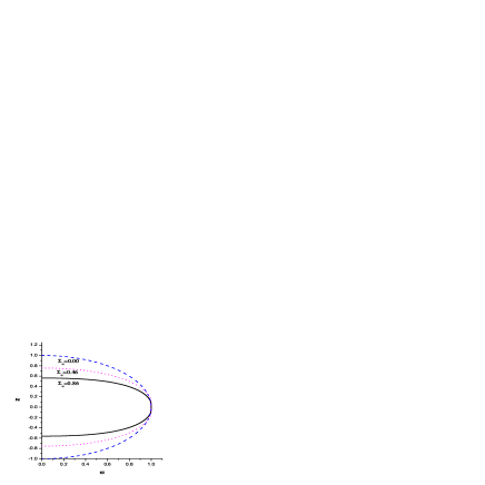
Figure 4: Typical (axi-symmetric) equilibrium figures of rotating drops for case I (one non-vanishing angular momentum), in $D=4$. The (blue) dashed line corresponds to a spherical surface with $\Sigma_{a}=0$. The (magenta) dotted line corresponds to $\Sigma_{a}=0.46$ and the (black) solid line corresponds to the limit $\Sigma_{a}=0.86$. In all three cases the equatorial radius is unity.

Numerical results for $D=4$ are shown in Figure 4 for some values of $\Sigma_{s}$, which can be compared to the $D=3$ results presented by Chandrasekhar in chandra . For $\Sigma_{a}=0$, the non-rotating case, we start by verifying numerically that the sphere is a solution, as it should, with $P_{0}a/T=D-1$. The equilibrium figures are very similar and indeed the similarity seems to continue for larger $D$. The three different equilibrium shapes shown in Figure 4 all enclose the origin. As in the $D=3$ case (see chandra ), we find that for $\Sigma_{a}$ larger than a certain critical value, the drop no longer enclosed the origin, giving rise to toroidal shapes. The condition to be satisfied at the critical $\Sigma$ is that $z=0$ at $r=0$. For $D=3$ the critical value of $\Sigma_{a}$ is $\Sigma_{a}\sim 2.32911$. For $D>3$ it is harder to determine the critical parameter, since there is no integral expression for the shape. Nevertheless we determine $\Sigma_{\rm crit}\sim 2.3$ for $D=4,5$ with a $5\%$ uncertainty. An open important problem is to determine if a critical point exists for all $D$. If not, this might mean that the bifurcation curve 1 does not bend down, and therefore that the angular momentum is unbounded, which might be a good analogue for what happens with ultra-rotating myersperry black holes. This may require more accurate numerical integrations, since we cannot trust our method for $D>5$.

V.2 Case II. All angular momenta coincident, and $D$ odd.

In case II we will find that the results are very similar to those for $D=3$. From equations (22), (34), (35) we find

$$P_{0}+\frac{1}{2}\rho\Omega^{2}\varpi^{2}=-\frac{T}{\varpi^{D-2}}\frac{d}{d\varpi}\left(\frac{\varpi^{D-2}\phi}{\sqrt{1+\phi^{2}}}\right)\,,$$ (65)

which is immediately integrated to give

$$P_{0}\frac{\varpi^{D-1}}{D-1}+\frac{\rho\Omega^{2}\varpi^{D+1}}{2(D+1)}=-\frac{T\varpi^{D-2}\phi}{\sqrt{1+\phi^{2}}}+C\,,$$ (66)

where $C$ is a constant.

Let’s first suppose the drop encloses the origin. In this case, there are points where $\varpi=0$ and therefore we must have $C=0$. Equation (66) can then be written as

$$P_{0}\frac{\varpi}{D-1}+\frac{\rho\Omega^{2}\varpi^{3}}{2(D+1)}=-\frac{T\phi}{\sqrt{1+\phi^{2}}}\,.$$ (67)

At the equator, where $\varpi=a$ we must have $\phi\rightarrow-\infty$ and then (66) implies that

$$\frac{P_{0}a}{(D-1)T}=1-\Sigma_{b}\,,\quad\Sigma_{b}\equiv\frac{\rho\Omega^{2}a^{3}}{2(D+1)T}\,.$$ (68)

Equations (67)-(68) are the same as equations (A4)-(A5) by Chandrasekhar chandra . So, figures of equilibrium enclosing the origin do not depend on the dimensionality of spacetime, if measured in terms of the dimensionless number $\Sigma_{b}$ (by this we mean of course that $z(\varpi,\Sigma_{b})$ is independent of $D$; anyway, the relation between $\Sigma_{b}$ and $\Omega$ depends on $D$, thus $z(\varpi,\Omega)$ depends on $D$). By measuring $\varpi$ and $\phi$ in units of $a$, we get

$$\phi=\frac{df}{d\varpi}=-\frac{\varpi\left(1-\Sigma_{b}+\Sigma_{b}\varpi^{2}\right)}{\sqrt{1-\varpi^{2}\left(1-\Sigma_{b}+\Sigma_{b}\varpi^{2}\right)^{2}}}\,,$$ (69)

which can be written as

$$z=f(\varpi)=\int_{\varpi}^{1}\frac{w\left(1-\Sigma_{b}+\Sigma_{b}w^{2}\right)}{\sqrt{1-w^{2}\left(1-\Sigma_{b}+\Sigma_{b}w^{2}\right)^{2}}}dw\,.$$ (70)

Transforming to a new variable $\theta$ defined through

$$\varpi^{2}=1-A\tan^{2}({\theta/2})\,,\quad A\equiv\frac{\sqrt{1+2\Sigma_{b}}}{\Sigma_{b}}\,,$$ (71)

the integral representation can be simplified to

$$z=\frac{1}{2\Sigma_{b}\sqrt{A}}\int_{0}^{\phi}\left(1+A\Sigma_{b}-\frac{2A\Sigma_{b}}{1+\cos{\theta}}\right)\frac{d\theta}{\sqrt{1-\chi^{2}\sin^{2}\theta}}\,,$$ (72)

where

$$\chi^{2}=\frac{1}{2}\left[1+\frac{1}{A}\left(\frac{1}{2}+\frac{1}{\Sigma_{b}}\right)\right]\,.$$ (73)

Here, $\phi$ is related to the value of $\varpi$ at the boundary by

$$\varpi=\sqrt{1-A\tan^{2}{\phi/2}}$$ (74)

The solution (72) can be expressed in terms of elliptic integrals

$$F(\chi,\phi)=\int_{0}^{\phi}\frac{d\theta}{\sqrt{1-\chi^{2}\sin^{2}\theta}}\,,\quad E(\chi,\phi)=\int_{0}^{\varpi}d\theta\sqrt{1-\chi^{2}\sin^{2}\theta}\,,$$ (75)

as

$$z=\frac{1}{2\Sigma_{b}\sqrt{A}}\left[\left(1-\Sigma_{b}A\right)F(\chi,\phi)+2A\Sigma_{b}\left(E(\chi,\phi)-\frac{\sin\phi\sqrt{1-\chi^{2}\sin^{2}\phi}}{1+\cos\phi}\right)\right]\,.$$ (76)

Some representative equilibrium solutions are displayed in Figure 5, for some values of $\Sigma_{b}$. The shapes are very similar to their “case I” relatives. We show typical shapes for high values of $\Sigma$ (these can be compared with the ones presented in Figure 1 of Chandrasekhar chandra ).

We have been dealing with drops that enclose the origin, and found that a closed expression for the shape is given by (76). When does this sequence end? A necessary and sufficient condition for the drop to enclose the origin is that $z=0$ and $\xi=0$ are simultaneously satisfied. Now, the condition $\xi=0$ implies that $\phi=\phi_{\rm max}=2\arctan A^{-1/2}$. Substituting this value in (76) we get

$$\Sigma_{\rm max}=2.32911\,.$$ (77)

For values of $\Sigma_{b}$ larger than the above, the figure no longer encloses the origin.

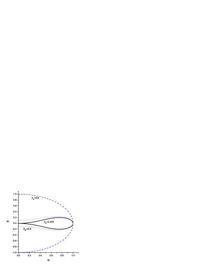
Figure 5: Typical equilibrum figures of rotating drops. The (blue) dashed line corresponds to a spherical surface with $\Sigma_{b}=0$. The (magenta) dotted line corresponds to $\Sigma_{b}=2$ and the (black) solid line corresponds to the limit $\Sigma_{b}=2.329$. In all three cases the equatorial radius was chosen to be unity.

VI Equilibrium toroidal shapes

In the general case of figures which do not enclose the origin (i.e.,$\varpi=0$ is not attained), we have to use equation (59) and (66) for cases I and II respectively. Here we shall focus on case II, equation (66), since it is easily manageable. In three spatial dimensions, solutions to equation (66) include ellipsoids, disks, biconcave and torus-like (or “wheels” in the terminology of rotatingdropexperiments2 ) forms heine ; rotatingdropexperiments2 . We now wish to consider if one can use these toroidal fluid configuration to model strong gravity configurations with the same topology. In particular, we consider a torus with a large radius $R$ and small thickness $r_{+}$ (the reason being that it is in this regime that one really expects a “pure” torus).

We will first look for torus-like solutions which start smoothly (i.e. $\phi=0$) at some distance $R_{1}$. We will call these “type A” toroidal solutions. The outer radius will be denoted $R_{2}$, where $\phi=-\infty$. In this case, we can easily determine the constants $p_{0}\,,C$ and write (66) as

$$P_{0}\frac{\varpi^{D-1}-R_{1}^{d-1}}{T(D-1)}+\frac{\rho\Omega^{2}\left(\varpi^{D+1}-R_{1}^{D+1}\right)}{2T(D+1)}=-\frac{\varpi^{D-2}\phi}{\sqrt{1+\phi^{2}}}\,,$$ (78)

where

$$P_{0}\frac{R_{2}^{D-1}-R_{1}^{D-1}}{T(D-1)}=R_{2}^{D-2}-\frac{\rho\Omega^{2}\left(R_{2}^{D+1}-R_{1}^{D+1}\right)}{2T(D+1)}\,.$$ (79)

We have numerically integrated equation (79) for several values of the parameters, and we find the law

$$R_{2}\left(R_{2}-R_{1}\right)^{2}(D+1)\Lambda\simeq 3.57\,,$$ (80)

which is independent of dimensionality $D$. Here

$$\Lambda\equiv\frac{\rho\Omega^{2}}{2T(D+1)}\,.$$ (81)

The meridional cross-section for a typical type A torus is displayed in Fig. 6.

Figure 6: Typical “smooth” Type A torus-like equilibrium shape. We have taken $D=4$ and $\Lambda=3.5,\,R_{1}=99.9549,\,R_{2}=100$.

As shown by Gulliver gulliver and Smith and Ross smithross there are several possible families of toroidal fluids (some of which have been experimentally observed already, see rotatingdropexperiments2 ). We have just described one of those families, that starts smoothly at $R_{1}$.

We can find a second family, the type B toroidal shape, which is more similar to the gravitational Dyson rings which will be described in Section X. What we now look for is a family which starts “abruptly” at $R_{1}$. Our numerical experiments seem to suggest a very rich behavior for the members of this family. For very small $\Lambda$, we find the following approximate scaling law,

$$r_{+}R^{2}\Lambda\sim\frac{1.96}{D+1}\,,\quad R\equiv R_{2}\sim R_{1}\,.$$ (82)

and the meridional cross-section of a typical member of this family is shown in Figure 7. Such a family seems to have been discussed already by Appell appell .

Figure 7: Typical Type B torus-like equilibrium shape. We have taken $D=4$ and $\Lambda=10^{-7},\,R_{1}=2\times 10^{4},\,R_{2}=2.00000099\times 10^{4}$. We chose $\frac{P_{0}}{T(D-1)}=1$.

Let’s pause a moment on this scaling law. If, following the suggestion in cardosodiasglrp , we try to model gravitating black bodies with fluids held together by surface tension, the first law suggests cardosodiasglrp that the surface tension is the equivalent of the Hawking temperature (up to a multiplicative constant). Now, the temperature of a black hole scales as $1/r$, where $r$ is some typical radius. For large “black rings” the relevant radius is the thickness $r_{+}$ of the ring. Thus we set $T\sim 1/r_{+}$. Using (81) and (82) we get

$$R^{2}\Omega^{2}\frac{M}{Rr_{+}^{D-3}}\sim 1\,,$$ (83)

where we replaced $\rho=M/V$.

On the other hand, the mass per unit length of such a “black torus” should be given by the mass of a $D-1$ Tangherlini black hole tangherlini (i.e., a higher dimensional non-rotating black hole):

$$(D-2)C_{D}GM\sim 4\pi(D-2)C_{D-2}R\,r_{+}^{D-3}\,.$$ (84)

Using the “constitutive” relation (84) for black objects and $J\sim\Omega MR$ we get finally

$$\frac{J^{2}}{M^{2}R^{2}}\sim 1\,.$$ (85)

Fortunately, there is an exact solution of Einstein’s equations describing a general relativistic black ring, in five dimensions ($D=4$) Emparan:2001wn : the black ring solution by Emparan and Reall Emparan:2001wn . The black ring solution is described by two parameters $\nu$ and $R$. They are characterized by having mass and angular momentum equal to Emparan:2001wn ; Elvang:2003mj :

$$M = \frac{3\pi R^{2}}{4G_{L}}\frac{\bar{\lambda}(1+\bar{\lambda})}{1+\nu}\,$$ (86)

$$J = \frac{\pi R^{3}}{2G_{L}}\frac{\sqrt{\bar{\lambda}\nu}(1+\bar{\lambda})^{5/2}}{(1+\nu)^{2}}\,.$$ (87)

Here, the parameter $\bar{\lambda}=2\nu/(1+\nu^{2})$ for black rings. Large rings can be obtained by setting $\nu\rightarrow 0$, in which case $R$ can be looked at as the radius of the ring. For very small $\nu$ we then have

$$\frac{J}{MR}=\frac{\sqrt{2}}{3}\,,$$ (88)

This is consistent with relation (85) obtained in the model of a fluid held together by surface tension. The case $D=3$ seems to be special for in three dimensions there are no black strings (all black holes must be topological spherical in this case), whereas the surface tension model seems to allow for rings;

VII Stability analysis of a rotating drop in case I. one non-vanishing angular momentum

To complete our discussion on drops held by surface tension, we consider the generalization to $D$-spatial dimensions of Figure 1, the bifurcation and stability diagram. Here we restrict ourselves to case I, i.e. only one non-vanishing angular momentum, corresponding to rotation in the plane $x^{1}-x^{2}$, and we will necessarily leave many topics for future research. For instance, all asymmetric figures will be left out of this exercise. We will follow the approach of Chandrasekhar chandra , based on the formalism of virial tensors. The special case in which the rotation is zero, i.e., a spherical drop, is considered in Appendix A where we compute the oscillation modes of a $D$-dimensional incompressible fluid sphere held by surface tension.

We have found the basic equations describing the equilibrium shape of rotating drops in the previous Sections. We would now like to investigate if these shapes are stable. The formalism to do this was laid down in Section IV.3, and equations (55)-(58) are the most general set of equations describing perturbed rotating drops.

From now on we will restrict our analysis to a special kind of perturbations, termed “toroidal” modes by Chandrasekhar chandra . The reason is that these modes are expected to play a role in the bifurcation and stability analysis. Future work should include an analysis of the other modes (termed “transverse-shear” and “pulsation modes”). We refer the reader to the work by Chandrasekhar chandra for further details on the formalism. The toroidal modes are defined by

$$\xi^{1} = \alpha x^{1}+\beta x^{2}$$

$$\xi^{2} = \beta x^{1}-\alpha x^{2}$$

$$\xi^{A} = 0$$ (89)

with $\alpha,\beta$ constant parameters.

As shown in the Appendix D, if a perturbation has the form (89), the only non-vanishing virial integrals are

$$\Gamma^{1;1} = -\Gamma^{2;2}=\pi\rho\alpha\frac{C_{D-2}}{D-2}\int_{0}^{a}\varpi^{3}\left[f(\varpi)\right]^{D-2}d\varpi$$ (90)

$$\Gamma^{1;2} = \Gamma^{2;1}=\pi\rho\beta\frac{C_{D-2}}{D-2}\int_{0}^{a}\varpi^{3}\left[f(\varpi)\right]^{D-2}d\varpi$$ (91)

where $\varpi=a$ is the intersection of the surface of the drop with the $x^{1}-x^{2}$ plane. These quantities satisfy the equations (55), which have the form

$$\omega^{2}\Gamma^{1;1}-2\omega\Omega\Gamma^{2;1} = \delta{\mathfrak{S}}^{11}+\Omega^{2}\Gamma^{11}+\delta\Pi\,,$$ (92)

$$\omega^{2}\Gamma^{2;2}+2\omega\Omega\Gamma^{1;2} = \delta{\mathfrak{S}}^{22}+\Omega^{2}\Gamma^{22}+\delta\Pi\,,$$ (93)

$$\omega^{2}\Gamma^{1;2}-2\omega\Omega\Gamma^{2;1} = \delta{\mathfrak{S}}^{12}+\Omega^{2}\Gamma^{12}\,,$$ (94)

$$\omega^{2}\Gamma^{2;1}+2\omega\Omega\Gamma^{1;2} = \delta{\mathfrak{S}}^{21}+\Omega^{2}\Gamma^{21}$$ (95)

and, combined, become

$$\frac{1}{2}\omega^{2}\left(\Gamma^{11}-\Gamma^{22}\right)-2\omega\Omega\Gamma^{12} = \delta{\mathfrak{S}}^{11}-\delta{\mathfrak{S}}^{22}+\Omega^{2}\left(\Gamma^{11}-\Gamma^{22}\right)\,,$$ (96)

$$\omega^{2}\Gamma^{12}+\omega\Omega\left(\Gamma^{11}-\Gamma^{22}\right) = 2\delta{\mathfrak{S}}^{12}+2\Omega^{2}\Gamma^{12}\,.$$ (97)

In order to solve equations (96), (97), where the virial integrals are given by (90), (91), we have to compute the surface integrals $\delta\mathfrak{S}^{12}$ and $\delta\mathfrak{S}^{11}-\delta\mathfrak{S}^{22}$.

In the case of perturbations of the form (89), they are (see Appendix D)

$$\delta\mathfrak{S}^{12} = -\frac{T}{2}\beta\pi C_{D-2}\int_{0}^{a}d\varpi\phi\varpi^{4}Q(\varpi)[f(\varpi)]^{D-3}$$ (98)

$$\delta\mathfrak{S}^{11}-\delta\mathfrak{S}^{22} = -T\alpha\pi C_{D-2}\int_{0}^{a}d\varpi\phi\varpi^{4}Q(\varpi)[f(\varpi)]^{D-3}\,.$$ (99)

where

$$Q=\frac{1}{\varpi^{2}}\left(\frac{\phi^{\prime}(\phi^{2}-2)}{(1+\phi^{2})^{5/2}}+\phi\frac{2+3\phi^{2}}{\varpi(1+\phi^{2})^{3/2}}-\frac{D-3}{z}\frac{\phi^{2}}{(1+\phi^{2})^{3/2}}\right)\,.$$ (100)

Therefore equations (96), (97) are equivalent to

$$\omega^{2}\alpha-2\omega\Omega\beta = -2{\mathfrak{I}}\alpha+2\Omega^{2}\alpha$$

$$\omega^{2}\beta+2\omega\Omega\alpha = -2{\mathfrak{I}}\beta+2\Omega^{2}\beta$$ (101)

where

$${\mathfrak{I}}\equiv\frac{T(D-2)}{4\rho}\frac{\int_{0}^{a}\phi\varpi^{4}Q(\varpi)[f(\varpi)]^{D-3}d\varpi}{\int_{0}^{a}\varpi^{3}\left[f(\varpi)\right]^{D-2}d\varpi}\,.$$ (102)

Setting $\omega^{2}=-\sigma^{2}$, the algebraic system (101) admits solutions

$$\sigma=\Omega\pm\sqrt{2{\mathfrak{I}}-\Omega^{2}}\,.$$ (103)

A neutral mode of oscillation ($\sigma=0$) occurs at $\Omega^{2}={\mathfrak{I}}$, but (in the absence of dissipative mechanisms as stressed in chandra ) the drop is still stable in the vicinity of this point. If

$$\Omega^{2}\leq 2{\mathfrak{I}}\,,$$ (104)

then $\sigma$ is real and the perturbation is stable; if the rotation frequency of the drop is larger, then the drop is unstable against toroidal perturbations. To ascertain stability or instability, we thus have to use the results of section V.1 for the equilibrium figures of rotating drops and insert the numerically generated shapes $z=z(\varpi)$ in (102) and (103).

If we measure $\varpi$ and $z$ in units of $a$ and $\Omega$ in units of $\sqrt{\frac{8T}{\rho a^{3}}}$ we get

$$\sigma=\sqrt{\Sigma_{a}}\pm\sqrt{2J-\Sigma_{a}}\,,$$ (105)

where the dimensionless quantity $J$ is

$$J\equiv\frac{(D-2)}{32}\frac{\int_{0}^{a}\phi\varpi^{4}Q(\varpi)[f(\varpi)]^{D-3}d\varpi}{\int_{0}^{a}\varpi^{3}\left[f(\varpi)\right]^{D-2}d\varpi}\,.$$ (106)

The results of solving (105) are displayed in Fig. 8 for $D=4$, which is a first step towards reconstructing the whole bifurcation diagram. In Fig. 8, $\sigma_{1}$ is (for real solutions) the largest of the two roots in (105) , i.e., as long as $2J>\Sigma_{a}$. For $2J<\Sigma_{a}$, we display only one root (the other root is the complex conjugate of this) by plotting the real and imaginary components of $\sigma$.

In three dimensions ($D=3$) it was found by Chandrasekhar chandra that rotating drops exhibit a neutral mode of oscillation at $\Sigma=0.4587$. He also found that rotating drops become unstable for $\Sigma>0.84$. We find that for general $D$ the results are similar. For instance, in $D=4$ there is a neutral mode of oscillation at $\Sigma_{a}=0.46$, and above the critical $\Sigma_{a}=0.86$ the drops are unstable.

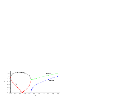
Figure 8: The dependence on the quantity $\Sigma$ of the characteristic frequencies of the toroidal modes of a rotating four-dimensional drop in $D=4$. The diagram is very similar to the three dimensional one ($D=3$) presented in Figure 3 of Chandrasekhar chandra . As a check on our numerical code, we verify that in the non-rotating limit our numerical results agree well with the analytical prediction $\sigma=\sqrt{D+1}/2$.

The shapes of the drops at these values of $\Sigma$ are displayed in Figure 4. Results for higher $D$ are very similar. Our numerical method only allowed to probe dimensions up to $D=6$, for larger $D$ we loose accuracy and the results cannot be trusted.

VIII Stability of fluid cylinders held by surface tension: the Rayleigh-Plateau instability

To end our discussion on fluids held by surface tension and also as a warm up exercise for the up-coming Sections, we will review the results of cardosodiasglrp , describing a simple capillary instability - the Rayleigh-Plateau instability rayleigh ; tomotika - as a good model for the Gregory-Laflamme instability. Most calculations were omitted in cardosodiasglrp so we present the full detailed computations here.

VIII.1 Rayleigh-Plateau instability in higher dimensions

We take an infinite non-rotating cylinder of radius $R_{0}$ held together by surface tension (therefore without self-gravity). Neglecting the external pressure, the unperturbed configuration is worked out easily to yield an internal pressure $P_{0}=(D-2)T/R_{0}$, where $D$ is the total number of spatial dimensions. We perturb slightly this configuration, according to

$$r=R_{0}+\epsilon e^{\omega t+ikz}\,.$$ (107)

The equations governing small perturbations are

$$P_{0}+\delta P = T{\rm div}\vec{n}\,,$$ (108)

$$\frac{\partial\bf u}{\partial t} = -{\rm grad}\Upsilon\,,$$ (109)

$${\rm div}{\bf u} = 0\,,$$ (110)

$$\Upsilon \equiv \frac{\delta P}{\rho}\,,$$ (111)

where $P_{0}$ is the pressure in the undisturbed cylinder and ${\bf u}$ is the fluid velocity. For instance, $u_{r}$ is the radial component of the velocity vector. Equation (109) yields

$$u_{r} = -\frac{1}{\omega}\frac{d}{dr}\Upsilon\,,$$ (112)

$$u_{z} = \frac{-ik}{\omega}\Upsilon\,.$$ (113)

Equation (110) implies that

$$\frac{du_{r}}{dr}+\frac{D-2}{r}u_{r}+\frac{du_{z}}{dz}=0\,.$$ (114)

Substituting in this the relations (112) and (113) we get

$$\frac{d^{2}\Upsilon}{dr^{2}}+\frac{D-2}{r}\frac{d\Upsilon}{dr}-k^{2}\Upsilon=0\,,$$ (115)

with (well-behaved at the origin) solution

$$\Upsilon=Cr^{3/2-D/2}I_{\alpha}(kr)\,,$$ (116)

where $\alpha=(D-3)/2$. By relation (112) we get

$$u_{r}=-C\frac{r^{3/2-D/2}}{\omega}\left(\frac{3-D}{2r}I_{\alpha}(kr)+kI^{\prime}_{\alpha}(kr)\right)\,,$$ (117)

where $I^{\prime}_{\alpha}(x)$ stands for the derivative of the Bessel function with respect to the argument $x$. Now, for this velocity to be compatible with the radial perturbation (107) one must clearly have

$$\epsilon\,e^{\omega t+ikz}=-C\frac{R_{0}^{3/2-D/2}}{\omega^{2}}\left(\frac{3-D}{2R_{0}}I_{\alpha}(kR_{0})+kI^{\prime}_{\alpha}(kR_{0})\right)\,.$$ (118)

With the displacement (107) we have to first order in $\epsilon$

$$\frac{\delta P}{\rho}=-\frac{T}{R_{0}^{2}\rho}\left(D-2-(kR_{0})^{2}\right)\epsilon e^{\omega t+ikz}\,.$$ (119)

Using (116) and (118) together with (111), (119) we finally find

$$R_{0}^{2}\omega^{2}=\frac{T}{\rho}\frac{\left(\frac{3-D}{2R_{0}}I_{\alpha}(kR_{0})+kI^{\prime}_{\alpha}(kR_{0})\right)}{I_{\alpha}}\left(D-2-(kR_{0})^{2}\right)\,,$$ (120)

where $I^{\prime}_{\alpha}(x)$ stands for the derivative of the Bessel function with respect to the argument $x$. This is the sought relation yielding the characteristic frequencies of an infinite cylinder of fluid held by surface tension. Formula (120) constitutes a generalization of a classic result by Rayleigh rayleigh , and it predicts that for $kR_{0}<\sqrt{D-2}$ the cylinder is unstable against this kind of “beaded” perturbations. In Figure 9 we show $\omega$ as function of wavenumber $k$ for several space dimensions $D$ (actually what is shown in the plots are dimensionless quantities $\omega R_{0}$ and $kR_{0}$).

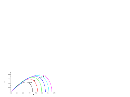
Figure 9: The Rayleigh-Plateau instability of a hyper-cylinder held together by surface tension, in several dimensions. Here the effective density were chosen to match those of a higher-dimensional non-rotating black hole. The instability gets stronger as the spacetime dimensionality increases, and the critical wavenumber (for which $\omega=0$) increases with $D$.

In Section IX we will discuss this instability in more detail, when we compare it to its self-gravitating counter-part.

VIII.2 Rayleigh-Plateau and Gregory-Laflamme

In General Relativity, there is an interesting class of black objects (objects with an event horizon) without spherical topology, the black branes horowitzstrominger . A broad class of these objects are unstable against gravity, in a mechanism known as Gregory-Laflamme (GL) instability gl . This is a beaded instability that makes any small perturbation with wavelength $\lambda$ of the order of, or larger than, the radius of the cylinder $R_{0}$ grow exponentially with time. It is a very robust long-wavelength instability. In cardosodiasglrp it was proposed to mimic the GL instability with the Rayleigh-Plateau instability, based on the suggestive appearance of the second law of black hole mechanics which endows the horizon with an effective surface tension. It was found that all aspects of the GL instability could be accounted for by the Rayleigh-Plateau instability in fluid cylinders. In some sense, the effective surface tension can mimic all gravitational aspects of black strings. If this is indeed correct, we should be able to predict the effects of rotation and charge on the GL instability, as discussed in the following.

VIII.2.1 Effects of magnetic fields

Even though not pursued here, a generalization for charged and/or rotating cylinders is of interest. In any case, we can lean on the four-dimensional results ($D=3$ spatial dimensions), for which the charged and rotating cases have been worked out chandrabookstability ; interfacial . A magnetic field has a stabilizing effect chandrabookstability , which is in agreement with the fully relativistic results for the Gregory-Laflamme instability, where it has been shown that adding charge to the black strings stabilizes it gl . There is good evidence that extremal charged black strings are marginally stable, and indeed in the capillary case (cylinder held by surface tension) it is possible to completely stabilize the cylinder if the magnetic field has a certain strength chandrabookstability (dependent on the conductivity of the fluid), so this may simulate the marginal stability of extremal black strings very well gl . Nevertheless an extension of the calculations presented here to the case of magnetically charged cylinders with surface tension is needed.

VIII.2.2 Effects of rotation

The effects of rotation on the capillary Rayleigh-Plateau instability can be discussed more intuitively. The centrifugal force, scaling with $r$, contributes with a de-stabilizing effect since there is an increased pressure under a crest but a reduced pressure under a trough. So in principle, the threshold wavelength should be smaller interfacial , i.e., the instability should get stronger when rotation is added. It is natural to expect that rotation will lift the degeneracy of the modes and that unstable modes will in general be non axi-symmetric. What can we expect for the general relativistic GL instability once rotation is added? A very naive reasoning is that since extremal charged black strings are marginally stable then perhaps the same happens with rotation, and so rotation has a stabilizing effect. This is incorrect as a simple argument shows. Consider a rotating black string in $D+1$ spacetime dimensions (with again $D$ being the number of spatial dimensions) of the form

$$g={\rm Kerr}^{D}\times{\bf R}\,,$$ (121)

where ${\rm Kerr}^{D}$ is the metric of higher dimensional Myers-Perry rotating black hole in $D$ spacetime dimensions, with only one angular momentum parameter (case I). If we focus on $D>4$ the angular momentum of these black holes is unbounded and one can show emparanmyers that for very large angular momentum

$${\rm Kerr}^{D}\sim S_{chw}^{D-2}\times{\bf R^{2}}\,,{\rm for\,\,large\,\,rotation}$$ (122)

where $S_{chw}^{D-2}$ is the metric of a higher dimensional Schwarzschild black hole, often referred to as Tangherlini tangherlini black holes. We thus finally get

$${\bf g}=S_{chw}^{D-2}\times{\bf R^{3}}\,,$$ (123)

This is the metric of a non-rotating black membrane in $D+1$ spacetime dimensions extended along the $3$ dimensions. But this is precisely the geometry considered by Gregory and Laflamme gl , and so it is unstable. While this argument says little about the strength of the instability as function of rotation, it does predict that rotating branes are still unstable. Putting this and the fluid membrane argument together we predict that rotation makes the GL instability stronger. One can also use an entropy argument, similar to the one in mu-inpark , to show that rotating black strings should be unstable. Again, an extension of the calculations presented in Section VIII.1 to the case of rotating cylinders with surface tension is needed. The $D=3$ case, studied in surfacetensionrotating , indicates that other effects may come into play with rotation. For instance, other instabilities seem to manifest themselves for high enough rotation, so this is a particularly exciting topic to consider.

Part II Fluids held by (Newtonian) self-gravity

IX Stability of self-gravitating fluid cylinders: the Dyson-Chandrasekhar-Fermi instability

It is only appropriate that we start the study of self-gravitating fluids by examining the (self-gravitating) counterpart of the cylinder studied in the last Section VIII.

A simple consistent solution can be found in $D$-dimensions, which corresponds to a static self-gravitating infinite cylinder made of fluid with a density $\rho$. For the moment we will not consider rotational effects (these will be discussed later), and we will focus on incompressible fluids. The stability of such a solution for the case of 3 spatial dimensions was studied for the first time by Chandrasekhar and Fermi chandrafermi (see also chandrabookstability ), who showed that such a solution is unstable against cylindrically symmetric perturbations (those for which the cross-section is still a circle, with a $z-$dependent radius), and stable against all others. If the radius of the cylinder is $R_{0}$, this “varicose” instability (in Chandrasekhar’s chandrabookstability terminology) sets in for wavelengths $\lambda>2\pi R/1.0668$.

A similar phenomenon had however been studied already in 1892 by Dyson dyson , who investigated the stability of self-gravitating rings of fluid. In his terminology, the ring is stable against fluted (the ring remains symmetrical about its axis but the cross-section is deformed) and twisted (the cross-section remains circular but the circular axis of the ring is deformed) perturbations. He also showed that sufficiently thin rings are unstable against a third kind of perturbation, so-called beaded perturbations (those for which the circular axis is undisturbed, but the cross-section is a circle of variable radius). But these correspond precisely to Chandrasekhar-Fermi type of perturbation (with the added bonus that Dyson effectively shows that the instability goes away if the length of the cylinder or ring is less than the critical wavelength), and thus we shall refer to this classical fluid instability as the Dyson-Chandrasekhar-Fermi (DCF) instability.

IX.1 A self-gravitating, non-rotating $D$-dimensional fluid cylinder

We will now generalize the DCF instability for an arbitrary number of dimensions. Consider an infinite cylinder of incompressible fluid, with density $\rho$ and radius $R$. To fix conventions we consider spacetime with $1$ (time)$+1$ (axis of cylinder)$+D-1=D+1$ total number of spacetime dimensions. In the following the coordinates $r\,,z$ have their usual meaning in polar coordinates. The gravitational potential ${\cal B}({\bf x})$ inside and exterior to the cylinder satisfies respectively

$$\nabla^{2}{\cal B}({\bf x})^{i} = -(D-2)C_{D}G\rho\,,$$ (124)

$$\nabla^{2}{\cal B}({\bf x})^{e} = 0\,.$$ (125)

Now, in $D$ spatial dimensions with cylindrical symmetry we have

$$\nabla^{2}=\frac{1}{r^{D-2}}\frac{d}{dr}\left(r^{D-2}\frac{d}{dr}\right)+\frac{d^{2}}{dz^{2}}\,.$$ (126)

Since we consider a cylinder with constant radius (along the axis in the $z$-direction), the last term drops off and we get the following solution (we demand that both the potential and its derivative be continuous throughout)

$${\cal B}({\bf x})^{i}_{0} = -\frac{(D-2)C_{D}G\rho}{2(D-1)}r^{2}\,,$$ (127)

$${\cal B}({\bf x})^{e}_{0} = -\frac{(D-2)C_{D}}{2}G\rho R_{0}^{2}\log r/R_{0}-\frac{D-2}{4}C_{D}G\rho R_{0}^{2}\,,\quad D=3\,.$$ (128)

$${\cal B}({\bf x})^{e}_{0} = -\frac{(D-2)C_{D}G\rho R_{0}^{2}}{2(D-1)}\left(\frac{D-1}{(D-3)}-\frac{2R_{0}^{D-3}}{(D-3)r^{D-3}}\right)\,,\quad D>3\,.$$ (129)

Hydrostatic equilibrium demands that the pressure $P_{0}$ satisfies

$$\frac{d}{dr}\left(\frac{P_{0}}{\rho}-{\cal B}({\bf x})\right)=0\,,$$ (130)

which yields, upon requiring $P_{0}(r=R_{0})=0$,

$$P_{0}=-\frac{(D-2)C_{D}G_{L}\rho^{2}}{2(D-1)}(r^{2}-R_{0}^{2})\,.$$ (131)

IX.2 Axisymmetric perturbations

Figure 10: Black strings and fluid cylinders are unstable to perturbations on the extended dimension, i.e., along the axis of the cylinder. Ripples propagating along this axis grow exponentially with time for wavelengths of order of the radius of the cylinder.

Suppose now the system is subjected to a perturbation (see Fig. 10) such that the boundary is described by

$$r=R_{0}+\epsilon e^{\omega t+ikz}\,.$$ (132)

The equations governing small perturbations are

$$\nabla^{2}\delta{\cal B}({\bf x}) = 0\,,$$ (133)

$$\frac{\partial\bf u}{\partial t} = -{\rm grad}\Upsilon\,,$$ (134)

$${\rm div}{\bf u} = 0\,,$$ (135)

$$\Upsilon \equiv \frac{\delta P}{\rho}-\delta{\cal B}({\bf x})^{i}\,.$$ (136)

Here ${\bf u}$ stands for the velocity of the perturbed fluid. Let’s solve for the first of these equations. When solving for the gravitational potential, the last term in (126) cannot be neglected. We find

$${\cal B}({\bf x})^{e} = {\cal B}({\bf x})^{e}_{0}+A\epsilon e^{\omega t+ikz}r^{3/2-D/2}K_{\alpha}(kr)\,,$$ (137)

$${\cal B}({\bf x})^{i} = {\cal B}({\bf x})^{i}_{0}+B\epsilon e^{\omega t+ikz}r^{3/2-D/2}I_{\alpha}(kr)\,,$$ (138)

where

$$\alpha=\frac{D-3}{2}\,,$$ (139)

and $K_{\alpha}$ and $I_{\alpha}$ are Bessel functions of argument $\alpha$. The constants $A$ and $B$ are determined by requiring continuity of the potential and its derivative on the boundary. By keeping only dominant terms in $\epsilon$ we find

$$A = (D-2)C_{D}G\rho R_{0}I_{\alpha}(kR_{0})\,,$$ (140)

$$B = (D-2)C_{D}G\rho R_{0}K_{\alpha}(kR_{0})\,.$$ (141)

Therefore we have

$$\delta{\cal B}({\bf x})^{i}=\epsilon(D-2)C_{D}G\rho R_{0}K_{\alpha}(kR_{0})e^{\omega t+ikz}r^{3/2-D/2}I_{\alpha}(kr)\,.$$ (142)

We also have $u\sim e^{i\omega t+ikz}$, therefore Eq. (134) yields

$$u_{r} = -\frac{1}{\omega}\frac{d}{dr}\Upsilon\,,$$ (143)

$$u_{z} = \frac{-ik}{\omega}\Upsilon\,.$$ (144)

(Here $u_{r}$, for instance, is the radial component of the velocity vector). Equation (135) implies that

$$\frac{du_{r}}{dr}+\frac{D-2}{r}u_{r}+\frac{du_{z}}{dz}=0\,.$$ (145)

Substituting the relations (143) and (144) we get

$$\frac{d^{2}\Upsilon}{dr^{2}}+\frac{D-2}{r}\frac{d\Upsilon}{dr}-k^{2}\Upsilon=0\,,$$ (146)

with (well-behaved at the origin) solution

$$\Upsilon=Cr^{3/2-D/2}I_{\alpha}(kr)\,.$$ (147)

By relation (143) we get

$$u_{r}=-C\frac{r^{3/2-D/2}}{\omega}\left(\frac{3-D}{2r}I_{\alpha}(kr)+kI^{\prime}_{\alpha}(kr)\right)\,,$$ (148)

where $I^{\prime}_{\alpha}(x)$ stands for the derivative of the Bessel function with respect to the argument $x$. Now, for this velocity to be compatible with the radial perturbation (132) one must clearly have

$$\epsilon\,e^{\omega t+ikz}=-C\frac{R_{0}^{3/2-D/2}}{\omega^{2}}\left(\frac{3-D}{2R_{0}}I_{\alpha}(kR_{0})+kI^{\prime}_{\alpha}(kR_{0})\right)\,.$$ (149)

Our problem is completely specified once we impose the boundary condition that the pressure must vanish at the boundary,

$$\delta P+\epsilon\frac{\partial P_{0}}{\partial r}=0\,,\Rightarrow\rho\Upsilon+\rho\delta{\cal B}({\bf x})^{i}+\epsilon\frac{\partial P_{0}}{\partial r}=0\,.$$ (150)

This gives us finally

$$\frac{\omega^{2}}{(D-2)C_{D}G\rho}=\frac{(3-D)I_{\alpha}(kR_{0})+kR_{0}I^{\prime}_{\alpha}(kR_{0})}{2I_{\alpha}(kR_{0})}\left(I_{\alpha}(kR_{0})K_{\alpha}(kR_{0})-\frac{1}{D-1}\right)\,.$$ (151)

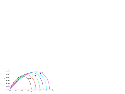
Figure 11: The DCF instability of a self-gravitating hyper-cylinder in several dimensions. Here the effective densities were chosen to match those of a higher-dimensional non-rotating black hole. The instability gets stronger as the spacetime dimensionality increases, and the critical wavenumber (for which $\omega=0$) increases with $D$.

In Fig. 11 we plot the dispersion relation $\omega(k)$ for several values of the dimensionality $D$, using Eq. (151). When $D$ increases the maximum $\omega$ grows which means that the instability gets stronger with space dimensionality. The threshold wavenumber $k_{c}$, defined as the wavenumber for which $\omega=0$, also increases with $D$. In Table 1 we present the threshold wavenumber for selected values of $D$.

Table 1: Dimensionless threshold wavenumber $kR_{0}$ for the DCF instability of a higher dimensional fluid cylinder, and the corresponding threshold wavenumber for Rayleigh-Plateau and Gregory-Laflamme instability (these last data are taken from kolsorkin ). The cylinder has $D-1$ dimensions with radius $R_{0}$ plus an extended direction along $z$. For $D=3$, not shown in the Table, we get $kR_{0}=1.06672$, in complete agreement with Chandrasekhar and Fermi’s chandrafermi result.

$D$	4	5	6	7	8	9	49	99
DCF	1.41	1.70	1.96	2.20	2.41	2.61	6.85	9.85
Rayleigh-Plateau	1.41	1.73	2.00	2.24	2.45	2.66	6.78	9.80
Gregory-Laflamme	0.876	1.27	1.58	1.85	2.09	2.30	6.72	9.75

For large $D$ we can obtain an analytical expression for the threshold wavenumber. In fact we can expand the Bessel functions as stegun :

$$I_{\alpha}(kR_{0}) \sim (kR_{0}/2)^{\alpha}\left(\frac{1}{\alpha!}+\frac{(kR_{0})^{2}}{4(\alpha+1)!}\right)\,,$$ (152)

$$K_{\alpha}(kR_{0}) \sim \frac{1}{2}(kR_{0}/2)^{-\alpha}\left((\alpha-1)!-\frac{(\alpha-2)!(kR_{0})^{2}}{4}\right)\,.$$ (153)

We get

$$K_{\alpha}(kR_{0})I_{\alpha}(kR_{0})-\frac{1}{D-1}\sim\frac{2}{D^{2}}-\frac{(kR_{0})^{2}}{4\alpha^{3}}\,\Rightarrow\,\,kR_{0}\sim\sqrt{D}\,.$$ (154)

A comparison between these results and the ones in Section VIII is instructive. The Figs. 9 and 11 show a remarkably similar behavior for both these instabilities. The threshold wavenumber (for which $\omega=0$), shown in Table 1 is also very similar to the corresponding one in both the Gregory-Laflamme and the Rayleigh-Plateau instability. Finally the $D\rightarrow\infty$ limit of the three instabilities is the same, $kR_{0}\sim\sqrt{D}$, in the sense that the threshold wavenumber coincides in this limit.

IX.3 DCF and Gregory-Laflamme

In cardosodiasglrp , the authors proposed to mimic the GL instability with the Rayleigh-Plateau instability, based on the suggestive appearance of the second law of black hole mechanics which endows the horizon with an effective surface tension. What we now propose is that, while the fluid membrane analogy is extremely powerful (and perhaps more trustworthy when it comes to mimic black objects), the Newtonian classical counterpart of the GL instability is the DCF instability. The GL instability should be the limit of the DCF instability when the density is so large that the cylinder is in fact a black string. Not only are the details of the DCF instability very similar to the GL instability (for instance, compare Figure 11 with Figure 1 of gl ) but for large $D$ we get exact agreement for the threshold wavenumber. In Table 1 we compare the threshold wavenumber for the three different types of instabilities (DCF, Rayleigh-Plateau and GL). The agreement is indeed very good, thus providing a convincing evidence for our conjectured analogy between DCF/Rayleigh-Plateau instabilities for fluids and GL instability for black strings.

It has been shown by Chandrasekhar and Fermi chandrafermi (see also Chandrasekhar chandrabookstability ) that the DCF instability is rooted in the sign change of potential energy for these varicose or beaded perturbations. But this is precisely what happens for the capillary of Rayleigh-Plateau instability (see Section VIII and discussion in cardosodiasglrp ), which explains why both of them yield so similar results. This is another pleasant indication that these instabilities are related. Based on this agreement we can discuss what to expect for rotating and charged cylinders and discuss the significance of the results for the GL instability.

IX.4 Effects of rotation and magnetic fields

Even though not pursued here, a generalization for charged and/or rotating cylinders is of great interest. In any case, we can lean on the four-dimensional results ($D=3$ spatial dimensions), for which the charged chandrabookstability ; chandrafermi ; shivamoggi and rotating cases karnik ; robe ; luyten have been worked out.

It has been shown that a magnetic field has a stabilizing effect, reducing the threshold wavenumber, i.e., increasing the minimum wavelength at which instability occurs. This is in agreement with the fully relativistic results for the Gregory-Laflamme instability, where it has been shown that adding charge to the black string stabilizes it gl . There is good evidence that the extremal case is marginally stable, and this could be perhaps the only real signature of an event horizon , because in the horizonless, Newtonian case, “no magnetic field, however strong, can stabilize the cylinder for disturbances of all wavelengths: the gravitational instability of long waves will persist” chandrabookstability . As we discussed in Section VIII, a capillary model may be more accurate to describe extremal objects.

Focusing now on the effect of rotation, it has been shown karnik (in three spatial dimensions) that rotation has a destabilizing effect. This agrees with the phenomenological arguments in cardosodiasglrp for cylinders held by surface tension (see also interfacial ) of the capillary model. It also agrees with the arguments in Section VIII suggesting that rotating black strings are unstable and thus a solid conjecture is that the Gregory-Laflamme instability of black strings gets stronger if one adds rotation. Stronger here means the threshold wavenumber decreases (the threshold wavelength increases). An interesting extension of the results presented here would be to consider a $D$-dimensional rotating cylinder of fluid.

X Self-gravitating torus and black rings

Toroidal shapes are thought to be common configurations in the universe. In some of them these rings or tori are associated with a massive central object, such as Saturn’s rings, whereas in others the central object plays almost no role at all (see wong and references therein). Toroidal configurations in full general relativity are also important (see ansorgringblackhole ), and they sometimes appear in the form of temporary black toroids, having an event horizon, in simulations of collapse of rotating matter shapiro .

The problem of a self-gravitating torus in Newtonian theory was investigated by many authors, the first studies belonging to Poincaré, Kowalewsky history and Dyson dyson . Dyson dyson considers a self-gravitating ring of radius $R$ and thickness $2r_{+}$ (i.e. the cross-section of the ring is a circle with radius $r_{+}$). For small $r_{+}/R$ he finds a power series solution (the leading term had already been derived by Poincaré and Kowalewsky history ) to the equilibrium problem as

$$\frac{\Omega^{2}}{\pi G_{L}\rho}=\frac{r_{+}^{2}}{R^{2}}\left(\log\left(\frac{8R}{r_{+}}\right)-\frac{5}{4}\right)-\frac{r_{+}^{4}}{8R^{4}}\left(\log\left(\frac{8R}{r_{+}}\right)-\frac{5}{12}\right)+{\cal O}(r_{+}/R)^{5}\,,\quad D=3\,.$$ (155)

To generalize this result to arbitrary dimensions we first observe that the gravitational potential of a very large ring of radius $R$ can be obtained by using as gaussian surface a torus. We get, for $D>3$,

$${\cal B}({\bf x})\sim-\frac{(D-2)C_{D}GM}{4\pi(D-3)C_{D-2}Rr_{+}^{D-3}}\,,\quad D>3\,,$$ (156)

where we expressed everything in terms of the physically more significant quantity $M$, the total mass of the ring. For rings with a large radius $R$ the hydrostatic equilibrium condition can be written as dyson ; chandrabookellipsoidal $\Omega^{2}R^{2}\sim{\cal B}({\bf x})$. This gives us

$$\Omega^{2}R^{2}\sim\frac{(D-2)C_{D}M}{4\pi(D-3)C_{D-2}R\,r_{+}^{D-3}}$$ (157)

It seems plausible that this formula also describes general relativistic objects, as long as one uses an “equation of state” to deduce $r_{+}$ in terms of the other quantities. This is because we are considering large rings, without really appealing to the internal structure of the object. For large rings, the dominating force determining equilibrium should be well-described by Newtonian forces, even though general relativistic effects become important “locally” and therefore it is the latter that determine $r_{+}(R,M)$. To plug-in the information that we are dealing with a black object, we use the relation between $r_{+}$, $M$ and $R$. For a black ring, the mass per length should be given, to a good accuracy, by the mass of a $D-1$ Tangherlini black hole tangherlini :

$$(D-2)C_{D}GM\sim 4\pi(D-2)C_{D-2}R\,r_{+}^{D-3}\,.$$ (158)

Using (157) and re-expressing everything in terms of the angular momentum $J\sim MR^{2}\Omega$ we get

$$\frac{J^{2}}{M^{2}R^{2}}\sim 1\,.$$ (159)

We can compare this prediction against the exact general relativistic black ring solution Emparan:2001wn in five spacetime dimensions ($D=4$). For large black rings, Eq. (88), $\frac{J}{MR}=\frac{\sqrt{2}}{3}$, in very good agreement with the Newtonian prediction (159). Moreover these arguments also lead to conjecture the existence of black rings in higher dimensions. Again the case $D=3$ seems special for there are Dyson rings in this case (actually that’s the case where they were found), albeit with a peculiar logarithmic term. As we remarked at the end of Section VI there are no black rings in $D=3$ so this is an instance where the analogy breaks down. To end this section, we note that another accurate and simple model was put forward by Hovdebo and Myers Hovdebo:2006jy to describe black rings in quasi-Newtonian terms, starting from the black string solution. Their conclusions are basically the same as ours, with the exception that instead of working with Newtonian forces, they extremize the entropy of the solution.

XI Self-gravitating, rotating spheroids: the MacLaurin sequence

To complete our discussion of self-gravitating objects, we consider the generalization to $D$-spatial dimensions of the simplest rotating objects: the MacLaurin sequence. Here we restrict ourselves to case of one non-vanishing angular momentum (case $I$ in the notation of Section II), corresponding to rotation in the plane $x^{1}-x^{2}$; the coordinates are then decomposed as (7)

$$x^{i}=(x^{a},x^{A})~{};~{}~{}~{}a=1,2~{};~{}~{}A=3,\dots,D\,.$$ (160)

We will follow the approach of Chandrasekhar chandrabookellipsoidal , based on the formalism of virial tensors. The special case in which the rotation is zero (i.e., a self-gravitating globe), is considered in Appendix B, where we compute the oscillation modes of a $D$-dimensional incompressible fluid sphere.

XI.1 The MacLaurin sequence in three dimensions

Here we briefly review the classical calculation of the MacLaurin sequence due to Chandrasekhar. We refer to chandrabookellipsoidal for further details.

Let us consider a matter distribution, inside the volume $V$, with density $\rho(\vec{x})$. Its gravitational potential is

$${\cal B}(\vec{x})\equiv G\int_{V}\frac{\rho(\vec{x}^{\prime})}{|\vec{x}-\vec{x}^{\prime}|}d^{3}x^{\prime}\,.$$ (161)

We define the tensor

$${\cal B}_{ij}(\vec{x})\equiv G\int_{V}\rho(\vec{x}^{\prime})\frac{(x^{i}-x^{\prime i})(x^{j}-x^{\prime j})}{|\vec{x}-\vec{x}^{\prime}|^{3}}d^{3}x^{\prime}\,,$$ (162)

which satisfies ${\cal B}_{ii}={\cal B}$. We also consider the potential energy

$$I\!{\cal B}\equiv-\frac{1}{2}\int_{V}\rho(\vec{x}){\cal B}(\vec{x})d^{3}x\,,$$ (163)

and the tensor

$$I\!{\cal B}_{ij}\equiv-\frac{1}{2}\int_{V}\rho(\vec{x}){\cal B}_{ij}(\vec{x})d^{3}x\,.$$ (164)

The following relation holds:

$$I\!{\cal B}_{ij}=\int_{V}\rho\frac{\partial{\cal B}}{\partial x^{i}}x^{j}d^{3}x\,.$$ (165)

Indeed,

$$\int_{V}\rho\frac{\partial{\cal B}}{\partial x^{i}}x^{j}d^{3}x=-G\int_{V}d^{3}x\int_{V}d^{3}x^{\prime}\rho(\vec{x})\rho(\vec{x}^{\prime})\frac{x^{i}-x^{\prime i}}{|\vec{x}-\vec{x}^{\prime}|^{3}}x^{j}=G\int_{V}d^{3}x^{\prime}\int_{V}d^{3}x\rho(\vec{x}^{\prime})\rho(\vec{x})\frac{x^{i}-x^{\prime i}}{|\vec{x}-\vec{x}^{\prime}|^{3}}x^{\prime j}$$

$$=-\frac{1}{2}G\int_{V}d^{3}x\int_{V}d^{3}x^{\prime}\rho(\vec{x})\rho(\vec{x}^{\prime})\frac{(x^{i}-x^{\prime i})(x^{j}-x^{\prime j})}{|\vec{x}-\vec{x}^{\prime}|^{3}}\,.$$ (166)

A consequence of this formula is that $I\!{\cal B}_{ij}$ is symmetric in its indices.

We then have the equations of motion

$$\ddot{x}^{a} = -\frac{\partial P}{\partial x^{a}}+\Omega^{2}\rho x^{a}+2\rho\Omega\epsilon^{ab}\dot{x}^{b}+\rho\frac{\partial{\cal B}}{\partial x^{a}}\,,$$

$$\ddot{z} = -\frac{\partial P}{\partial z}+\rho\frac{\partial{\cal B}}{\partial z}\,,$$ (167)

where $z=x^{A}=x^{3}$.

At equilibrium,

$$\Omega^{2}\rho x^{a}-\frac{\partial P}{\partial x^{a}}+\rho\frac{\partial{\cal B}}{\partial x^{a}} = 0\,,$$

$$-\frac{\partial P}{\partial z}+\rho\frac{\partial{\cal B}}{\partial z} = 0\,.$$ (168)

We compute the virial integrals by multiplying equations (168) by $x^{j}$ and integrating in the volume domain $V$. The resulting integrals are:

$$\Omega^{2}\int_{V}d^{3}x\rho x^{a}x^{j} = \Omega^{2}I_{aj}\,,$$

$$-\int_{V}d^{3}x\frac{\partial P}{\partial x^{i}}x^{j} = \delta^{ij}\int_{V}d^{3}xP\equiv\delta_{ij}\Pi\,,$$

$$\int_{V}d^{3}x\rho\frac{\partial{\cal B}}{\partial x^{i}}x^{j} = I\!{\cal B}_{ij}\,.$$ (169)

Thus we get virial equations

$$\Omega^{2}I_{ab}+I\!{\cal B}_{ab} = -\Pi\delta_{ab}\,,$$

$$\Omega^{2}I_{a3}+I\!{\cal B}_{a3} = 0\,,$$

$$I\!{\cal B}_{3a} = 0~{}~{}~{}~{}~{}\hbox{(therefore $I\!{\cal B}_{a3}=I_{a3}=0$)}\,,$$

$$I\!{\cal B}_{33} = -\Pi\,.$$ (170)

The inertia tensor at equilibrium is then, in general,

$$I_{ij}=\left(\begin{array}[]{ccc}I_{11}&I_{12}&0\\ I_{21}&I_{22}&0\\ 0&0&I_{33}\\ \end{array}\right)\,.$$ (171)

We note that equilibrium does not require necessarily $I_{11}=I_{22}$.

From the virial equations we get

$$I\!{\cal B}_{11}+\Omega^{2}I_{11}=I\!{\cal B}_{22}+\Omega^{2}I_{22}=I\!{\cal B}_{33}\,.$$ (172)

There are two possible solutions of equations (172). The first is the simplest one, with

$$I_{11}=I_{22}\,,~{}~{}~{}~{}~{}I\!{\cal B}_{11}=I\!{\cal B}_{22}\,,$$ (173)

namely, with axial symmetry; the rotation frequency is given by

$$\Omega^{2}=\frac{I\!{\cal B}_{33}-I\!{\cal B}_{11}}{I_{11}}\,.$$ (174)

and can be easily computed; this solution corresponds to the MacLaurin sequence of oblate axially symmetric ellipsoids. The second, more complicate, has $I_{11}\neq I_{22}$, and corresponds to the Jacobi sequence of tri-axial ellipsoids; this solution exists only if the total angular momentum exceeds a critical value.

XI.2 The MacLaurin sequence in higher dimensions

The generalization of the three dimensional formalism to higher dimensions is more or less straighforward. Let us consider a matter distribution in $D$ dimensions, inside the volume $V$, with density $\rho(\vec{x})$. Again, we define the gravitational potential

$${\cal B}(\vec{x})\equiv G\int_{V}\frac{\rho(\vec{x}^{\prime})}{|\vec{x}-\vec{x}^{\prime}|^{D-2}}d^{D}x^{\prime}\,.$$ (175)

and

$${\cal B}_{ij}(\vec{x})\equiv\int_{V}\rho(\vec{x}^{\prime})\frac{(x^{i}-x^{\prime i})(x^{j}-x^{\prime j})}{|\vec{x}-\vec{x}^{\prime}|^{D}}d^{D}x^{\prime}\,,$$ (176)

which satisfies ${\cal B}_{ii}={\cal B}$. We also consider the potential energy

$$I\!{\cal B}\equiv-\frac{1}{2}\int_{V}\rho(\vec{x}){\cal B}(\vec{x})d^{D}x\,.$$ (177)

and the tensor

$$I\!{\cal B}_{ij}\equiv-\frac{1}{2}\int_{V}\rho(\vec{x}){\cal B}_{ij}(\vec{x})d^{D}x\,.$$ (178)

We can check that the following relation, which is the extension of (165), holds:

$$I\!{\cal B}_{ij}=\frac{1}{D-2}\int_{V}\rho\frac{\partial{\cal B}}{\partial x^{i}}x^{j}d^{D}x\,.$$ (179)

Indeed,

$$\int_{V}\rho\frac{\partial{\cal B}}{\partial x^{i}}x^{j}d^{D}x=-(D-2)G\int_{V}d^{D}x\int_{V}d^{D}x^{\prime}\rho(\vec{x})\rho(\vec{x}^{\prime})\frac{x^{i}-x^{\prime i}}{|\vec{x}-\vec{x}^{\prime}|^{D}}x^{j}=(D-2)G\int_{V}d^{D}x^{\prime}\int_{V}d^{D}x\rho(\vec{x}^{\prime})\rho(\vec{x})\frac{x^{i}-x^{\prime i}}{|\vec{x}-\vec{x}^{\prime}|^{D}}x^{\prime j}$$

$$=-\frac{D-2}{2}G\int_{V}d^{D}x\int_{V}d^{D}x^{\prime}\rho(\vec{x})\rho(\vec{x}^{\prime})\frac{(x^{i}-x^{\prime i})(x^{j}-x^{\prime j})}{|\vec{x}-\vec{x}^{\prime}|^{D}}\,.$$ (180)

Thus $I\!{\cal B}_{ij}$ is symmetric in its indices, as it was in three dimensions.

The equations of motion yield

$$\ddot{x}^{a} = -\frac{\partial P}{\partial x^{a}}+\Omega^{2}\rho x^{a}+2\rho\Omega\epsilon^{ab}\dot{x}^{b}+\rho\frac{\partial{\cal B}}{\partial x^{a}}\,,$$

$$\ddot{x}^{A} = -\frac{\partial P}{\partial x^{A}}+\rho\frac{\partial{\cal B}}{\partial x^{A}}\,.$$ (181)

At equilibrium we get,

$$\Omega^{2}\rho x^{a}-\frac{\partial P}{\partial x^{a}}+\rho\frac{\partial{\cal B}}{\partial x^{a}} = 0\,,$$

$$-\frac{\partial P}{\partial x^{A}}+\rho\frac{\partial{\cal B}}{\partial x^{A}} = 0\,.$$ (182)

We compute the virial integrals by multiplying equations (182) by $x^{j}$ and integrating in the volume domain $V$. The resulting integrals are:

$$\Omega^{2}\int_{V}d^{D}x\rho x^{a}x^{j} = \Omega^{2}I_{aj}\,,$$

$$-\int_{V}d^{D}x\frac{\partial P}{\partial x^{i}}x^{j} = \delta^{ij}\int_{V}d^{D}xP\equiv\delta_{ij}\Pi\,,$$

$$\int_{V}d^{D}x\rho\frac{\partial{\cal B}}{\partial x^{i}}x^{j} = (D-2)I\!{\cal B}_{ij}\,.$$ (183)

Thus we get the virial equations

$$\Omega^{2}I_{ab}+(D-2)I\!{\cal B}_{ab} = -\Pi\delta_{ab}\,,$$

$$\Omega^{2}I_{aA}+(D-2)I\!{\cal B}_{aA} = 0\,,$$

$$(D-2)I\!{\cal B}_{Aa} = 0~{}~{}~{}~{}~{}\hbox{(therefore $I\!{\cal B}_{aA}=I_{aA}=0$)}\,,$$

$$(D-2)I\!{\cal B}_{AB} = -\Pi\delta_{AB}\,.$$ (184)

The inertia tensor at equilibrium is then, in general,

$$I_{ij}=\left(\begin{array}[]{cccc}I_{11}&I_{12}&0&\\ I_{21}&I_{22}&0&\\ 0&0&I_{33}&\\ &&&\ddots\\ \end{array}\right)\,.$$ (185)

We note that equilibrium does not require necessarily $I_{11}=I_{22}$.

From the virial equations we get

$$(D-2)I\!{\cal B}_{11}+\Omega^{2}I_{11}=(D-2)I\!{\cal B}_{22}+\Omega^{2}I_{22}=(D-2)I\!{\cal B}_{33}=\dots=(D-2)I\!{\cal B}_{DD}\,.$$ (186)

The simplest solution of Eqs. (186) is the one with axial symmetry:

$$I_{11}=I_{22}\,,~{}~{}~{}~{}~{}I\!{\cal B}_{11}=I\!{\cal B}_{22}\,,,$$ (187)

which is the generalization of MacLaurin sequence; the rotation frequency is given by

$$\Omega^{2}=(D-2)\frac{I\!{\cal B}_{33}-I\!{\cal B}_{11}}{I_{11}}\,,$$ (188)

and can be easily computed. But equations (186) leave open the possibility to have other, non axisymmetric equilibrium configurations: the generalization of the Jacobi sequence. Their detailed study will have to wait for other, possible numerical, studies.

XII Concluding remarks

XII.1 Equilibrium configurations in higher dimensions

We have started the investigation of equilibrium figures of rotating fluids in higher dimensions. We used two appealingly simple models: one in which the fluid is held together by surface tension and the other in which self-gravity is the cohesive force. We have developed the basic tools to start an investigation of this important subject. Nevertheless, this work represents only a first step towards the understanding of the behavior of rotating fluids in higher dimensions. Many questions remain to be addressed. It is clear that the general behavior observed for $D=3$ still holds for higher $D$. It is natural to expect that (for instance for fluid drops), a non axisymmetric figure bifurcates from the point where the axisymmetric figure starts to be unstable, the point at which relation (104) saturates. What is the shape of this figure? Is the instability point really a bifurcation point? This would allow one to generalize Figure 2 to higher dimensions. Furthermore, our study must be extended to encompass more general perturbations and more general angular momentum configurations. Another pressing issue is to determine whether there is always a toroidal figure of equilibrium in general $D$ dimensions: could it be that for certain $D$ a drop always encloses the origin regardless of its rotation? If so, this could be an excellent model for ultra-rotating Myers-Perry black holes, for which the angular momentum is unbounded. Concerning self-gravitating spheroids, there are many more unanswered questions. The formalism to study self-gravitating fluid drops must be further developed to find the actual equilibrium shapes as well as their stability. This would lead to a generalization of the MacLaurin and Jacobi sequences to higher dimensions. It would also be exciting to study numerically self-gravitating toroidal configurations (the analogue of the Dyson rings).

XII.2 Fluids and black objects

XII.2.1 Mimicking event horizons with cohesive forces

The work presented here also allows one to better understand how gravity (even in the strong field regime) behaves in higher dimensions. Given the number of new solutions and instabilities discovered in this setting over the last few years, this is a particularly fascinating topic. A lesson to learn from the examples shown here (the Rayleigh-Plateau instability, the toroidal configurations, the DCF instability, the Dyson rings, etecetera) is that many attractive forces, like Newtonian gravity and surface tension, seem to mimic strong gravity situations very well. There is probably something more to it, when one shows that surface tension mimics so well the behavior of horizons, but this remains to be explained. A particularly promising proposal emparan , which gathers support from our work, is that the physics of fluids and black holes can be related semi-quantitatively for smooth enough objects. If the object is very inhomogeneous or is highly distorted, then the gravitational self-interaction between different parts of the object will be strong, and then one expects that the details of the (fully non-linear) dynamics of the interaction will matter. So, for very inhomogeneous objects, general relativity or fluid dynamics would yield very different results. This means that the fluid approach won’t, in principle, be useful for cases such as: the deeply non-linear evolution of the GL instability, when large inhomogeneities develop; the Myers-Perry black holes close to the extremal singularity (in the cases they admit a Kerr bound); thick black rings, and in general black rings in the region where non-uniqueness occurs. This is unfortunate since these are very intriguing and important regimes. Nevertheless, a plethora of important and smooth objects (like the ones studied here) should then be described by these very simple models, and could even be a starting point for more complex situations.

XII.2.2 The bifurcation diagram of black objects

In the Introduction, the suggestion is made that bifurcation diagram in Fig. 1 is in some sense universal, the qualitative behavior holding for most objects held together by some cohesive force. The natural generalization is to conjecture it may describe bifurcation diagrams of black objects. We would like to comment on the limitation of that generalization .

Kerr bound

The first point to address concerns the existence of a Kerr bound. If the bifurcation diagram Fig. 1 were indeed universal, the angular momentum of black holes would be bounded. In fact, the results in Section V imply that there is a bound on $J$ in any of the cases I and II. We know however that the angular momentum of black holes in “case I” is unbounded (for $D>4$) myersperry ; emparanmyers , whereas in case II it is bounded myersperry (see for instance Eq. 7 in Kunduri:2006qa ). Thus the surface tension model does not accurately describe ultra-spinning black holes, for the cases studied numerically ($D=3,4,5$). Accurate numerical results are needed for higher dimensions, as well as results for self-gravitating fluids. This would clear the issue.

Instabilities

The second point concerns the instability of the solutions. The results available in the literature concerning black hole instability can be summarized as

(i) For $D>4$, case I, there should be both axisymmetric and non-axisymmetric instabilities emparanmyers .

(ii) For $D=4$ spatial dimensions, case I, the analysis of emparanmyers does not apply; it was been suggested in Emparan:2001wn that there could be an axisymmetric instability before the Kerr bound, ending in a black ring.

(iii) For case II, the study in Kunduri:2006qa suggests no instability.

The studies in emparanmyers and Kunduri:2006qa focused only on a special kind of perturbation, related to a traceless tensor mode. This seems to belong to the same representation of our “toroidal mode”, even if one relates to the metric and the other to the fluid.

In Section VII we found that a “case I” rotating drop is unstable. This agrees with the black hole picture (i) above. We were not able to extend the discussion to rotating drops in case II. So far both pictures (black hole and fluids) agree. The long-known discrepancy is the $D=3$ case: Kerr black holes in $D=3$ spatial dimensions are stable, whereas the fluid picture would predict instability. Another point of discrepancy is that the most general vacuum solution of Einstein’s equations in $3$ spatial dimensions is the Kerr family, with spherical topology, so black rings are absent in this case. We can thus argue that $D=3$ is a remarkable exception.

Non-axisymmetric figures of equilibrium

The final point we would like to touch upon is the question of existence of non-axisymmetric figures of equilibrium. In the simple fluid models (see Figs. 1 and 3) there is a family of non-axisymmetric stationary figures; one of the main points of our paper was to show that this holds for fluids in general higher dimensions, too. We went on to find non-axisymmetric instability which we argued brings the drop to a non-axisymmetric stationary configuration (in the case of gravitating fluid, we proved that there exist stationary, non-axisymmetric configurations analogous to the Jacobi sequence). However, it is shown in Hollands:2006rj that higher dimensional rotating black objects must be axisymmetric. Therefore stationary non-axisymmetric black solutions do not exist, and one would be led to think that the bifurcation diagram for fluids is completely misleading.

The explanation for the disagreement is very simple, and lies in the fact that one is expecting from the model something it was not built to do: a more realistic analogy would have to take emission of gravitational waves into account, never considered up to now. Since non-axisymmetric objects radiate gravitational waves, we would not expect to find stationary equilibrium solutions of that kind. Indeed, for three spatial dimensions this problem was considered by Chandrasekhar chandragw . Chandrasekhar proved that when one takes emission of gravitational waves into account (all other “curved spacetime” effects being neglected), the Jacobi configuration is unstable and evolves in the direction of increasing angular velocity, approaching the bifurcation point. Furthermore, he proved that radiation reaction does not make the fluid unstable past the point of bifurcation. Thus the bifurcation diagram for black objects would be drawn by first deleting all the non-axisymmetric figures.

It is reasonable to think that this result, i.e. the non-existence of non-axisymmetric stationary fluid configurations in general relativity, can be generalized to higher dimensions. If this is the case, this would be the analogue of the no-go result of Hollands:2006rj for higher dimensional rotating black holes.

XII.3 Future work

The two examples we have studied (surface tension and self-gravitating fluids) can therefore improve and strengthen our understanding of black objects. The fact that rotating fluid drops develop instabilities at finite (usually small) rotation seems to suggest that black holes cannot have large rotation. This was also put forward by Emparan and Myers emparanmyers in connection with the Gregory-Laflamme instability. The examples shown here and the classical three-dimensional results discussed in the Introduction suggest that the final state of this instability is a non axi-symmetric figure. Some evidence was put forward already in emparanmyers and this work adds some more evidence to that possibility. In fact, it might not even be possible to find matter configurations with high enough rotation to form these ultra-spinning black holes following collapse: we prove in Appendix C that self-gravitating, rotating homogeneous fluids always have a bounded angular velocity (this is a generalization of a classic result by Poincaré). Future work along these lines (mimicking strong gravity situations with analogue models) could start by investigating the black string phase transition mu-inpark ; Gubser:2001ac ; Sorkin:2004qq within either the surface tension or the self-gravity models. Another potentially interesting topic would be to investigate the collapse of toroidal fluid configurations to form black rings.

Acknowledgements

We warmly thank Emanuele Berti, Marco Cavaglià, Óscar Dias, José Lemos and Mu-In Park for a careful and critical reading of the manuscript and for many useful comments. We are indebted to Roberto Emparan for very useful suggestions and specially for having enlightened us as to the significance of some of the results. We are also indebted to Dr. Claus-Justus Heine for very useful correspondence on this subject and for preparing Figure 2 for us. We thank Dr. Robert Brown for kind permission to use Figure 1 and Drs. Yoshiharu Eriguchi and Izumi Hachisu for kind permission to use Figure 3. VC acknowledges financial support from Fundação Calouste Gulbenkian through the Programa Gulbenkian de Estímulo à Investigação Científica.

Appendix A Oscillation modes of a spherical drop held together by surface tension

What are the oscillation modes of a spherical drop held together by surface tension? In three spatial dimensions the answer to this classical problem can be found for instance in lamb ; reid . We will now generalize it to an arbitrary number of dimensions. Take a spherical drop with radius $R_{0}$. Define again

$$\Upsilon\equiv\frac{\delta P}{\rho}\,,$$ (189)

where $\delta P$ is the change in pressure inside the drop (the outside pressure is taken to be zero), after it is perturbed by a displacement of the form

$$r=R_{0}+\epsilon e^{\omega t}Y({\rm angles})\,,$$ (190)

where $Y({\rm angles})$ are hyper-spherical harmonics, with eigenvalue $l(l+D-2)$. The equations governing small perturbations are

$$P_{0}+\delta P = T{\rm div}\vec{n}\,,$$ (191)

$$\frac{\partial\bf u}{\partial t} = -{\rm grad}\Upsilon\,,$$ (192)

$${\rm div}{\bf u} = 0\,,$$ (193)

$$\Upsilon \equiv \frac{\delta P}{\rho}\,.$$ (194)

With the displacement (190), equation (191) can be solved to yield (for details we refer the reader to Landau and Lifshitz reid ) near $r=R_{0}$ and to first order in $\epsilon$

$$\frac{\delta P}{\rho}=-\frac{T}{R_{0}^{2}\rho}(l-1)(l+D-1)\epsilon e^{\omega t}Y({\rm angles})\,.$$ (195)

Therefore

$$\Upsilon=-\frac{T(l-1)(l+D-1)}{\rho R_{0}^{l+2}}r^{l}\epsilon e^{\omega t}Y({\rm angles})\,.$$ (196)

On the other hand, observing that $\nabla^{2}\left(\frac{\delta P}{\rho}\right)=0$ we may immediately write

$$\frac{\delta P}{\rho}=\epsilon F_{p}\frac{r^{l}}{R_{0}^{l}}Y({\rm angles})e^{\omega t}\,,$$ (197)

with $F_{p}$ a constant to be determined. We thus have from the definition of $\Upsilon$ that

$$\Upsilon=\frac{r^{l}}{R_{0}^{l}}\epsilon\,F_{p}\,Y({\rm angles})e^{\omega t}\,.$$ (198)

Equation (192) then yields

$$u_{r}=-\frac{1}{\omega}\frac{d}{dr}\Upsilon\,,$$ (199)

Now, for this velocity to be compatible with the radial perturbation (190) one must have

$$F_{p}=-\frac{R_{0}\omega^{2}}{l}\,.$$ (200)

Inserting this in (198) and equating the resulting expression with (196) we get

$$\omega^{2}=-\frac{Tl(l-1)(l+D-1)}{\rho R_{0}^{3}}\,,$$ (201)

which is a generalization of the three-dimensional result found in lamb ; reid . Note that the drop is always stable ($\omega$ is imaginary) and that $l=0$ and $1$ modes do not exist. The first corresponds to spherically symmetric pulsation of the drop, which violates the constant volume assumption and the second corresponds to a translation of the drop as whole.

Appendix B Oscillation modes of a self-gravitating, non-rotating sphere

Here we analyze the modes of a self-gravitating fluid sphere, in which case we can do without the virial formalism and find an exact analytical expression for the oscillation frequencies. We aim at generalizing the four-dimensional result by Kelvin and others lamb . The analysis from Section IX carries over with minimal changes.

The gravitational potential ${\cal B}({\bf x})$ inside and outside the globe satisfy respectively

$$\nabla^{2}{\cal B}({\bf x})^{i} = -(D-2)C_{D}G\rho\,,$$ (202)

$$\nabla^{2}{\cal B}({\bf x})^{e} = 0\,.$$ (203)

In the unperturbed state we get

$${\cal B}({\bf x})^{i}_{0} = -\frac{(D-2)C_{D}G\rho}{2D}\left(-\frac{DR_{0}^{2}}{D-2}+r^{2}\right)\,,$$ (204)

$${\cal B}({\bf x})^{e}_{0} = \frac{C_{D}G\rho R_{0}^{D}}{D}\frac{1}{r^{D-2}}\,.$$ (205)

Hydrostatic equilibrium demands that the pressure $P_{0}$ satisfies

$$\frac{d}{dr}\left(\frac{P_{0}}{\rho}-{\cal B}({\bf x})\right)=0\,,$$ (206)

which yields, upon requiring $P_{0}(r=R_{0})=0$,

$$P_{0}=\frac{(D-2)C_{D}G\rho^{2}}{2D}(R_{0}^{2}-r^{2})\,.$$ (207)

Suppose now the system is subjected to a perturbation, of general form

$$r=R_{0}+\epsilon e^{\omega t}Y({\rm angles})\,,$$ (208)

where $Y({\rm angles})$ are hyper-spherical harmonics, with eigenvalue $l(l+D-2)$.

The equations governing small perturbations are

$$\nabla^{2}\delta{\cal B}({\bf x}) = 0\,,$$ (209)

$$\frac{\partial\bf u}{\partial t} = -{\rm grad}\Upsilon\,,$$ (210)

$${\rm div}{\bf u} = 0\,,$$ (211)

$$\Upsilon \equiv \frac{\delta P}{\rho}-\delta{\cal B}({\bf x})^{i}\,.$$ (212)

Here ${\bf u}$ stands for the velocity of the perturbed fluid. Let’s solve for the first of these equations. We find

$${\cal B}({\bf x})^{e} = {\cal B}({\bf x})^{e}_{0}+\epsilon Ar^{-l-D+2}Y({\rm angles})e^{\omega t}\,,$$ (213)

$${\cal B}({\bf x})^{i} = {\cal B}({\bf x})^{i}_{0}+\epsilon Br^{l}Y({\rm angles})e^{\omega t}\,.$$ (214)

The constants $A$ and $B$ are determined by requiring continuity of the potential and its derivative on the boundary. By keeping only dominant terms in $\epsilon$ we find

$$A = \frac{(D-2)C_{D}G\rho}{2l+D-2}R_{0}^{l+D-1}\,,$$ (215)

$$B = \frac{(D-2)C_{D}G\rho}{2l+D-2}R_{0}^{1-l}\,.$$ (216)

Therefore we have

$$\delta{\cal B}({\bf x})^{i}=\epsilon\frac{(D-2)C_{D}G\rho}{2l+D-2}R_{0}^{1-l}r^{l}Y({\rm angles})e^{\omega t}\,.$$ (217)

Observing that $\nabla^{2}\left(\frac{\delta P}{\rho}\right)=0$ we may immediately write

$$\frac{\delta P}{\rho}=\epsilon F_{p}\frac{r^{l}}{R_{0}^{l}}Y({\rm angles})e^{\omega t}\,,$$ (218)

with $F_{p}$ a constant to be determined. We thus have from the definition of $\Upsilon$, equation (212), that

$$\Upsilon\frac{r^{l}}{R_{0}^{l}}\epsilon\left(F_{p}-\frac{(D-2)C_{D}G\rho R_{0}}{2l+D-2}\right)Y({\rm angles})e^{\omega t}\,.$$ (219)

Equation (210) then yields

$$u_{r}=-\frac{1}{\omega}\frac{d}{dr}\Upsilon\,,$$ (220)

Now, for this velocity to be compatible with the radial perturbation (208) one must have

$$F_{p}=\frac{(D-2)C_{D}G\rho R_{0}}{2l+D-2}-\frac{R_{0}\omega^{2}}{l}\,.$$ (221)

Imposing a vanishing pressure on the surface of the globe we have finally

$$\omega^{2}=-\frac{2(D-2)C_{D}G\rho}{D}\frac{l(l-1)}{2l+D-2}\,,$$ (222)

which is a generalization of Kelvin’s four-dimensional result lamb to an arbitrary number of dimensions. As in the previous Section, the globe is always stable and $l=0$ and $l=1$ modes do not exist. Result (222) can be compared with the results for the modes of spherically symmetric black holes in higher dimensions modeshigherdim ; modeshigherdim2 .

Appendix C An upper bound for the rotation of an homogeneous fluid mass

In four dimensions there is an upper bound, derived by Poincaré poincaresurfacetension for the maximum angular velocity of a rigidly rotating, homogeneous fluid mass in equilibrium. Consider a region $V$ in three dimensional space bounded by a surface $S$. Let $\frac{\partial}{\partial n_{e}}$ denote differentiation of a function across $S$ in the direction of the unit normal $n_{e}$ outward from $V$. The divergence theorem states that for any (sufficiently smooth) vector field $\vec{W}$

$$\int_{S}\vec{W}.\vec{n}\,d\sigma=\int_{V}{\rm div}\vec{W}d^{3}x\,.$$ (223)

If we choose $\vec{W}={\rm grad}{\cal B}$, where ${\cal B}$ is the gravitational potential, we get

$$\int_{S}\frac{\partial{\cal B}}{\partial n_{e}}\,d\sigma=\int_{V}\nabla^{2}{\cal B}d^{3}x=-\int_{V}4\pi G\rho d^{3}x\,,$$ (224)

where we used Poisson’s equation in the last equality.

A necessary (but not sufficient) condition for equilibrium is that the force at every point in $S$ be directed inward. But the total force is $F_{r}=\frac{\partial U}{\partial n_{e}}$, where $U$ is the modified potential

$${\cal U}={\cal B}+\frac{1}{2}\Omega^{2}\left((x^{1})^{2}+(x^{2})^{2}\right)$$ (225)

(we choose $x^{3}=z$ to be the axis of rotation). We then must require

$$\frac{\partial{\cal U}}{\partial n_{e}}<0\,\,\Rightarrow\int_{S}\frac{\partial{\cal U}}{\partial n_{e}}d\sigma=\int_{V}\nabla^{2}Ud^{3}x=\int_{V}\left(-4\pi G\rho+2\Omega^{2}\right)d^{3}x<0\,.$$ (226)

thus we have the Poincaré’s inequality

$$\Omega^{2}<2\pi\rho G\,.$$ (227)

This derivation can be easily generalized to $D>3$ dimensional Euclidean space. If we assume the gravitational potential is (175)

$${\cal B}({\bf x})=G\int d^{D}x^{\prime}\frac{\rho({\bf x^{\prime}})}{|{\bf x}-{\bf x^{\prime}}|^{D-2}}\,,$$ (228)

then Poisson’s equation becomes

$$\nabla^{2}{\cal B}=-(D-2)C_{D}G\rho\,,$$ (229)

where

$$C_{D}=\frac{2\pi^{D/2}}{\Gamma\left(\frac{D}{2}\right)}\,,$$ (230)

and $C_{D}r^{D-1}$ is the area of the $(D-1)$-sphere. Indeed,

$$\int_{V}\nabla^{2}\left(\frac{1}{r^{D-2}}\right)d^{D}x=\int_{S}\frac{\partial}{\partial n_{e}}\left(\frac{1}{r^{D-2}}\right)d\sigma=-(D-2)\int_{S}\frac{x^{i}}{r^{D}}\frac{x^{i}}{r}d\sigma=-(D-2)C_{D}\,.$$ (231)

We now consider the two cases labeled by I and II, that is,

• one non-vanishing angular momentum;

• all angular momenta coincident, and $D$ odd.

The modified potential, in both cases, writes as

$${\cal U}={\cal B}+\frac{1}{2}\Omega^{2}\sum_{a}(x^{a})^{2}\,,$$ (232)

where $a=1,2$ in case I, $a=1,\dots,D-1$ in case II. Its Laplacian is

$$\nabla^{2}{\cal U} = -C_{D}\rho G+2\Omega^{2}~{}~{}~{}~{}~{}~{}~{}~{}~{}~{}~{}~{}\,\hbox{in case I}\,,$$

$$\nabla^{2}{\cal U} = -C_{D}\rho G+(D-1)\Omega^{2}~{}~{}~{}~{}~{}\hbox{in case II}\,,$$ (233)

therefore Poincaré’s inequality becomes

$$\Omega^{2} < \frac{C_{D}}{2}\rho G~{}~{}~{}~{}~{}\hbox{in case I}\,,$$

$$\Omega^{2} < \frac{C_{D}}{D-1}\rho G~{}~{}~{}~{}~{}\hbox{in case II}\,.$$ (234)

For angular velocities larger than this threshold, the gravitational pull is insufficient to balance the centrifugal force, and there body is disrupted.

Appendix D Toroidal perturbations of a rotating drop

Here we compute some useful quantities in the case of a rotating drop with one non-vanishing angular momentum, constant density $\rho$ and with toroidal perturbations (following the denomination of Chandrasekhar chandra ), i.e.

$$\xi^{a} = T^{ab}x^{b}\,,$$

$$\xi^{A} = 0\,,$$

$$T^{ab} = \left(\begin{array}[]{cc}\alpha&\beta\\ \beta&-\alpha\,,\\ \end{array}\right)\,,$$ (237)

with $\alpha,\beta$ constant parameters. We remind that, in the case with one non-vanishing angular momentum, the coordinates $\{x^{i}\}$ are decomposed as in (7), (8)

$$x^{i}=(x^{a},x^{A})~{};~{}~{}~{}~{}a=1,2~{};~{}~{}A=3,\dots,D$$ (238)

and we have defined

$$\varpi = \sqrt{(x^{1})^{2}+(x^{2})^{2}}\,,$$

$$z = \sqrt{(x^{3})^{2}+\dots+(x^{D})^{2}}\,,$$ (239)

so that

$$x^{1} = \varpi\cos\theta\,,$$

$$x^{2} = \varpi\sin\theta\,.$$ (240)

The $D$-dimensional volume integration element is

$$d^{D}x=\varpi z^{D-3}d\varpi d\theta dzd\Omega_{D-3}\,.$$ (241)

If we integrate on the angular variables, we get

$$\int_{S^{1}\times S^{D-3}}d^{D}x=2\pi C_{D-2}\varpi z^{D-3}d\varpi dz\,,$$ (242)

where $C_{D-2}$ is the area of a unit $(D-3)$-sphere (230).

Let us now consider the $(D-1)$-dimensional surface $S$ of equation $z=f(\varpi)$. Since on $S$, $dz=\phi d\varpi$, the metric element on $S$ is

$$d\sigma^{2}=(1+\phi)^{2}d\varpi^{2}+\varpi^{2}d\theta^{2}+[f(\varpi)]^{2}d\Omega_{D-3}^{2}\,.$$ (243)

The surface integration element is then

$$dS=\sqrt{1+\phi^{2}}\varpi[f(\varpi)]^{D-3}d\varpi d\theta d\Omega_{D-3}\,.$$ (244)

In particular, being

$$n^{a}=-\frac{\phi x^{a}}{\sqrt{1+\phi^{2}}\varpi}\,,$$ (245)

we have

$$dS^{a}=n^{a}dS=-\phi x^{a}[f(\varpi)]^{D-3}d\varpi d\theta d\Omega_{D-3}\,.$$ (246)

After integration on the $(D-3)$-sphere we get,

$$\int_{S^{D-3}}dS^{a}=-\phi x^{a}[f(\varpi)]^{D-3}C_{D-2}d\varpi d\theta\,.$$ (247)

Notice that in the $D=3$ case we have $dS^{a}=-2\phi x^{a}d\varpi d\theta$ where the factor $2$ accounts for the two hemispheres of the drop.

D.1 Virial integrals

We can easily compute the virial integrals

$$\Gamma^{i;j}=\int_{V}\rho\xi^{i}x^{j}d^{D}x\,.$$ (248)

From (237) it follows $\Gamma^{A;j}=0$; furthermore,

$$\int_{V}x^{i}x^{j}d^{D}x=0~{}~{}~{}~{}{\rm if}~{}i\neq j$$ (249)

because the drop is symmetric with respect to reflections to any axis, therefore $\Gamma^{a,A}=0$.

We have

$$\int_{V}(x^{1})^{2}d^{D}x = \left(\int_{0}^{2\pi}d\theta\cos^{2}\theta\right)C_{D-2}~{}\int_{0}^{a}d\varpi\varpi^{3}~{}\int_{0}^{f(\varpi)}dzz^{D-3}\,,$$ (250)

$$= \pi\frac{C_{D-2}}{D-2}\int_{0}^{a}d\varpi\varpi^{3}\left[f(\varpi)\right]^{D-2}=\int_{V}(x^{2})^{2}d^{D}x\,,$$

where $\varpi=a$ is the intersection of the drop with the $x^{1}-x^{2}$ plane (namely, $f(a)=0$); therefore,

$$\Gamma^{1;1} = -\Gamma^{2;2}=\pi\rho\alpha\frac{C_{D-2}}{D-2}\int_{0}^{a}\varpi^{3}\left[f(\varpi)\right]^{D-2}d\varpi\,,$$ (251)

$$\Gamma^{1;2} = \Gamma^{2;1}=\pi\rho\beta\frac{C_{D-2}}{D-2}\int_{0}^{a}\varpi^{3}\left[f(\varpi)\right]^{D-2}d\varpi\,.$$ (252)

We notice that these formulae are valid for every $D\geq 3$. When $D>3$, $C_{D-2}$ represents the area of the unit $(D-3)$-sphere; when $D=3$, the factor $C_{1}=2$ accounts for the two hemispheres composing the drop.

D.2 Surface energy integrals

Here we want to compute the quantities $\delta\mathfrak{S}^{12}$ and $\delta\mathfrak{S}^{11}-\delta\mathfrak{S}^{22}$ where (see (51))

$$\delta\mathfrak{S}^{ab}=-T\left[\int_{S}\xi^{b}n^{k}_{~{},k}dS^{a}+\int_{S}x^{b}\delta(n^{k}_{~{},k})dS^{a}-\int_{S}x^{b}n^{k}_{~{},k}\frac{\partial\xi^{c}}{\partial x^{a}}dS^{c}\right]\,,$$ (253)

and

$$dS^{a}=-\phi x^{a}[f(\varpi)]^{D-3}C_{D-2}d\varpi d\theta\,.$$ (254)

Being $\xi^{a}=T^{ab}x^{b}$, we have that

$$\int d\theta\left[\xi^{2}x^{1}-x^{2}\frac{\partial\xi^{c}}{\partial x^{1}}x^{c}\right]=\int_{0}^{2\pi}d\theta[T^{2a}x^{a}x^{1}-T^{1a}x^{2}x^{a}]=\int_{0}^{2\pi}d\theta\left((x^{1})^{2}-(x^{2})^{2}\right)\beta=0\,,$$

$$\int_{0}^{2\pi}d\theta\left[\xi^{1}x^{1}-\xi^{2}x^{2}-x^{1}\frac{\partial\xi^{c}}{\partial x^{1}}x^{c}+x^{2}\frac{\partial\xi^{c}}{\partial x^{2}}x^{c}\right]=\int_{0}^{2\pi}d\theta\left[T^{1a}x^{a}x^{1}-T^{2a}x^{a}x^{2}-x^{1}T^{c1}x^{c}+x^{2}T^{c2}x^{c}\right]=0\,.$$

therefore the first and third integrals in (253) cancel for the components $\delta\mathfrak{S}^{12}$ and $\delta\mathfrak{S}^{11}-\delta\mathfrak{S}^{22}$:

$$\delta\mathfrak{S}^{12} = -T\int_{S}\delta(n^{k}_{~{},k})x^{2}dS^{1}\,,$$

$$\delta\mathfrak{S}^{11}-\delta\mathfrak{S}^{22} = -T\int_{S}\delta(n^{k}_{~{},k})x^{1}dS^{1}-T\int_{S}\delta(n^{k}_{~{},k})x^{2}dS^{2}\,.$$ (255)

The perturbation of the divergence $\delta(n^{i}_{~{},i})$ is given by (54)

$$\delta(n^{i}_{~{},i}) = (\delta n^{i})_{,i}-\frac{\partial n^{i}}{\partial x^{k}}\frac{\partial\xi^{k}}{\partial x^{i}}=(\delta n^{a})_{,a}-T^{ab}n^{a}_{~{},b}+(\delta n^{A})_{,A}\,,$$

$$\delta n^{a} = \left(n^{k}n^{l}\frac{\partial\xi^{k}}{\partial x^{l}}\right)n^{a}-n^{j}\frac{\partial\xi^{j}}{\partial x^{a}}=[n^{b}n^{c}T^{bc}]n^{a}-T^{ab}n^{b}\,,$$

$$\delta n^{A} = \left(n^{k}n^{l}\frac{\partial\xi^{k}}{\partial x^{l}}\right)n^{A}=[n^{b}n^{c}T^{bc}]n^{A}\,.$$ (256)

with

$$n^{a}=-\phi\frac{x^{a}}{\varpi\sqrt{1+\phi^{2}}}\,,~{}~{}~{}~{}~{}n^{A}=\frac{x^{A}}{z\sqrt{1+\phi^{2}}}\,.$$ (257)

We have

$$n^{a}_{~{},b}=-\frac{\phi^{\prime}}{(1+\phi^{2})^{3/2}}\frac{x^{a}x^{b}}{\varpi^{2}}+\frac{\phi}{\sqrt{1+\phi^{2}}}\frac{x^{a}x^{b}}{\varpi^{3}}-\delta^{ab}\frac{\phi}{\sqrt{1+\phi^{2}}\varpi}\,,$$ (258)

then we find

$$\delta\left(n^{i}_{~{},i}\right)=-\frac{x^{a}x^{b}T^{ab}}{\varpi^{2}}\left[\frac{\phi^{\prime}(\phi^{2}-2)}{(1+\phi^{2})^{5/2}}+\phi\frac{2+3\phi^{2}}{\varpi(1+\phi^{2})^{3/2}}-\frac{D-3}{z}\frac{\phi^{2}}{(1+\phi^{2})^{3/2}}\right]\,.$$ (259)

Therefore,

$$\delta\left(n^{i}_{~{},i}\right)=-\left[\alpha\left((x^{1})^{2}-(x^{2})^{2}\right)+2\beta x^{1}x^{2}\right]Q(\varpi)=-\varpi^{2}\left(\alpha\cos 2\theta+\beta\sin 2\theta\right)Q(\varpi)\,,$$ (260)

where

$$Q=\frac{1}{\varpi^{2}}\left(\frac{\phi^{\prime}(\phi^{2}-2)}{(1+\phi^{2})^{5/2}}+\phi\frac{2+3\phi^{2}}{\varpi(1+\phi^{2})^{3/2}}-\frac{D-3}{z}\frac{\phi^{2}}{(1+\phi^{2})^{3/2}}\right)\,.$$ (261)

The surface integrals $\delta\mathfrak{S}^{12}$, $\delta\mathfrak{S}^{11}-\delta\mathfrak{S}^{22}$ are then

$$\delta\mathfrak{S}^{12} = TC_{D-2}\int_{0}^{a}d\varpi\int_{0}^{2\pi}d\theta\phi x^{1}x^{2}[f(\varpi)]^{D-3}\delta(n^{k}_{~{},k})\,,$$ (262)

$$= -\frac{T}{2}\beta\pi C_{D-2}\int_{0}^{a}d\varpi\phi\varpi^{4}Q(\varpi)[f(\varpi)]^{D-3}\,,$$

$$\delta\mathfrak{S}^{11}-\delta\mathfrak{S}^{22} = TC_{D-2}\int_{0}^{a}d\varpi\int_{0}^{2\pi}d\theta\phi\left[(x^{1})^{2}-(x^{2})^{2}\right][f(\varpi)]^{D-3}\delta(n^{k}_{~{},k})\,,$$ (263)

$$= -T\alpha\pi C_{D-2}\int_{0}^{a}d\varpi\phi\varpi^{4}Q(\varpi)[f(\varpi)]^{D-3}\,.$$

Appendix E Newton’s constant

Here we would like to relate our adopted definition of Newton’s constant to the one adopted in the by now classical work by Myers and Perry myersperry . They define a Newton’s constant $G_{MP}$ such that Einstein’s equations read

$$R_{\mu\nu}-\frac{1}{2}g_{\mu\nu}R=8\pi G_{MP}T_{\mu\nu}\,.$$ (264)

We will now derive “Newton’s law” from this equation, in order to relate the different Newton constants. To derive Newton’s law $a=-\nabla{\cal B}({\bf x})$, we consider the Newtonian limit of Einstein’s equation (slowly moving particles, weak and static gravitational fields).

A test particle follows the geodesics of the spacetime

$$\frac{d^{2}x^{\mu}}{d\tau^{2}}+\Gamma^{\mu}_{\rho\sigma}\frac{dx^{\rho}}{d\tau}\frac{dx^{\sigma}}{d\tau}=0\,.$$ (265)

Under the “moving slowly” condition $\frac{dx^{i}}{d\tau}\ll\frac{dt}{d\tau}$ this is simplified to

$$\frac{d^{2}x^{\mu}}{d\tau^{2}}+\Gamma^{\mu}_{00}\left(\frac{dt}{d\tau}\right)^{2}=0\,.$$ (266)

Due to the staticity assumption,

$$\Gamma^{\mu}_{00}=\frac{1}{2}g^{\mu\lambda}\left(\partial_{0}g_{\lambda 0}+\partial_{0}g_{0\lambda}-\partial_{\lambda}g_{00}\right)=-\frac{1}{2}g^{\mu\lambda}\partial_{\lambda}g_{00}\,,$$ (267)

so that the geodesic equation simplifies to

$$\frac{d^{2}x^{\mu}}{d\tau^{2}}-\frac{1}{2}g^{\mu\lambda}\partial_{\lambda}g_{00}\left(\frac{dt}{d\tau}\right)^{2}=0\,.$$ (268)

Lastly, the Newtonian limit implies weak gravitational fields, so we set

$$g_{\mu\nu}=\eta_{\mu\nu}+h_{\mu\nu}\,,\quad|h_{\mu\nu}|\ll 1\,.$$ (269)

Thus we have (we can show that to first order $g^{\mu\nu}=\eta^{\mu\nu}-h^{\mu\nu}$)

$$\Gamma^{\mu}_{00}=-\frac{1}{2}\eta^{\mu\lambda}\partial_{\lambda}h_{00}\,,$$ (270)

and therefore

$$\frac{d^{2}x^{\mu}}{d\tau^{2}}=\frac{1}{2}\eta^{\mu\lambda}\partial_{\lambda}h_{00}\left(\frac{dt}{d\tau}\right)^{2}\,.$$ (271)

Dividing the spatial components of this equation by $\left(\frac{dt}{d\tau}\right)^{2}$ we have finally

$$\frac{d^{2}x^{i}}{dt^{2}}=\frac{1}{2}\partial_{i}h_{00}\,,$$ (272)

which allows one to identify $h_{00}=-2{\cal B}({\bf x})$. On the other hand, from Myers and Perry’s equation (1.5), we get

$$\nabla^{2}h_{00}=-16\pi\frac{D-2}{D-1}G_{MP}\,.$$ (273)

Comparing our (229) with (273), we get the relation between our adopted $G$ and $G_{MP}$ as (there’s an extra minus sign that follows from the conventions adopted here for the relation force-potential)

$$C_{D}G=\frac{8\pi}{D-1}G_{MP}\,.$$ (274)

References

- (1) J. Plateau, Statique Expérimentale et Théorique des Liquides Soumis aux Seules Forces Moléculaires, (Paris, Gauthier-Villars, 1873).
- (2) C. P. Lee, A. V. Anilkumar, A. B. Hmelo and T. G. Wang, “Equilibrium of liquid drops under the effects of rotation and acoustic flattening: results from USML-2 experiments in space,” J. Fluid Mech. 354, 43 (1998).
- (3) P. Aussillous and D. Quéré, “Liquid marbles,” Nature 411, 925 (2001); idem, “Shapes of rolling liquid drops,” J. Fluid. Mech. 512, 133 (2004); idem, “Non-stick droplets,” Chem. Eng. Technol. 25, 9 (2002).
- (4) H. Poincaré, “Sur l’équilibre d une masse fluide animée d un mouvement de rotation,” Acta Mathematica 7, 259 (1885).
- (5) S. Chandrasekhar, “The stability of a rotating liquid drop,” Proc. Roy. Soc. Ser. A 286, 1 (1965).
- (6) R. A. Brown and L. E. Scriven, “The shape and stability of rotating liquid drops,” Proc. Roy. Soc. London Ser. A 371, 331 (1980).
- (7) R. A. Brown and L. E. Scriven, “New class of asymmetric shapes of rotating liquid drops,” Phys. Rev. Lett. 45, 180 (1980).
- (8) C. -J. Heine, “Computations of form and stability of rotating drops with finite elements,” IMA J. Numer. Anal. 26, 723 (2006).
- (9) R. Gulliver, “Tori of prescribed mean curvature and the rotating drop,” in E.H.A. Gonzales, I. Tamanini, ed.: Variational methods for equilibrium problems of fluids (Meeting held in Trento, Italy, from June 20 to 25, 1983), Asterisque 118, 167 (1984).
- (10) C.-J. Heine, Computations of form and stability of rotating drops with finite elements, PhD thesis, available at http://www.mathematik.uni-freiburg.de/IAM/homepages/claus/
- (11) A very complete account of the topic up to the late 19 century can be found in I. Todhunter, History of the mathematical theories of attraction and the figure of the earth (Dover, New York, 1962). Particular important works include H. Poincaré, Les méthodes nouvelles de la méchanique céleste (Gauthier-Villars, Paris, 1892, 1894, 1899); “Sur la stabilité de l anneau de Saturne,” C. R. Acad. Sci. 100, 346 (1885); idem, Bull. Astr. 2, 109 (1885); ibidem 2, 405 (1885); S. Kowalewsky, “Zusaetze und Bemerkungen zu Laplace s Untersuchungen ueber die Gestalt der Saturnringe,” Astron. Nachr. 111, 37 (1895); F. Tisserand, Traité de Méchanique Céleste (Gauthier-Villars, Paris, 1894).
- (12) S. Chandrasekhar, Ellipsoidal figures of equilibrium (Dover, New York, 1987); S. Chandrasekhar, Selected Papers, Volume 4 (The University of Chicago Press, Chicago, 1989).
- (13) A. Balaguera-Antolinez, D. F. Mota and M. Nowakowski, “Ellipsoidal configurations in the de Sitter spacetime,” Class. Quantum Grav. 23, 4497 (2006).
- (14) Y. Eriguchi and I. Hachisu, “New equilibrium sequences bifurcating from MacLaurin sequence,” Prog. Theor. Phys. 67, 844 (1982); Y. Eriguchi, I. Hachisu and D. Sugimoto, “Dumb-bell-shape equilibria and mass-shedding pear-shape of selfgravitating incompressible fluid,” Prog. Theor. Phys. 67, 1068 (1982);
- (15) J. M. Bardeen, “A reexamination of the post-newtonian MacLaurin spheroids,” Astrophys. J. 167, 425 (1971).
- (16) C-Y Wong, “Toroidal figures of equilibrium,” Astrophys. J. 190, 675 (1974).
- (17) Y. Eriguchi and D. Sugimoto, “Another equilibrium sequence of self-gravitating and rotating incompressible fluid,” Prog. Theor. Phys. 65, 1870 (1981).
- (18) F. W. Dyson, “The potential of an anchor ring,” Phil. Trans. Roy. Soc. 184, 43 (1893); F. W. Dyson, “The potential of an anchor ring. Part II,” Phil. Trans. Roy. Soc. 184A, 1041 (1893).
- (19) M. Ansorg, A. Kleinwächter and R. Meinel, “Uniformly rotating asisymmetric fluid configurations bifurcating from highly flattened MacLaurin spheroids,” Mon. Not. Roy. Astron. Soc. 339, 515 (2003);
- (20) N. Bohr and J. A. Wheeler, “The mechanism of nuclear fission,” Phys. Rev. 56, 426 (1939). See also C. Y. Wong, “Toroidal and spherical bubble nuclei,” Annals of Physics (NY) 77, 279 (1973).
- (21) W. J. Swiatecki, “The rotating charged or gravitating liquid drop and problems in nuclear physics and astronomy,” in Proceedings of the International Colloquium on Drops and Bubbles (ed. D. J. Collins, M. S. Plesset and M. M. Saffren, 1974), Jet Propulsion Laboratory, Pasadena California; S. Cohen, F. Plasil and W. J. Swiatecki, “Equilibrium configurations of rotating charged or gravitating liquid masses with surface tension. II.,” Annals of Physics (NY) 82, 557 (1974).
- (22) V. Cardoso and O. J. C. Dias, “Rayleigh-Plateau and Gregory-Laflamme instabilities of black strings,” Phys. Rev. Lett. 96, 181601 (2006).
- (23) K. S. Thorne, D. A. MacDonald and R. H. Price, Black Holes: The Membrane Paradigm (Yale University Press, 1986).
- (24) J. M. Bardeen, B. Carter and S. W. Hawking, “The four laws of black hole mechanics,” Commun. Math. Phys. 31, 161 (1973).
- (25) J. D. Bekenstein, “Black holes and entropy,” Phys. Rev. D 7, 2333 (1973).
- (26) S. W. Hawking, “Particle creation by black holes,” Commun. Math. Phys. 43, 199 (1975).
- (27) R. Defay, I. Prigogine, A. Bellemans and D. H. Everett, Surface tension and adsorption, (Joun Wiley and Sons, New York, 1966).
- (28) L. Smarr, “Mass formula for Kerr black holes,” Phys. Rev. Lett. 30, 71 (1973).
- (29) M. Parikh and F. Wilczek, “An action for black hole membranes,” Phys. Rev. D 58, 064011 (1998).
- (30) D. M. Eardley and S. B. Giddings, “Classical black hole production in high-energy collisions,” Phys. Rev. D 66, 044011 (2002).
- (31) G. ’t Hooft, “Dimensional Reduction in Quantum Gravity,” gr-qc/9310026; L. Susskind, “The World as a hologram,” J. Math. Phys. 36, 6377 (1995); J. M. Maldacena, “The Large N limit of superconformal field theories and supergravity,” Adv. Theor. Math. Phys. 2, 231 (1998); E. Witten, “Anti-de Sitter space and holography,” Adv. Theor. Math. Phys. 2, 253 (1998); R. Bousso, “A covariant entropy conjecture,” JHEP 9907, 004 (1999).
- (32) P. Kovtun, D. T. Son and A. O. Starinets, “Viscosity in strongly interacting quantum field theories from black hole physics,” Phys. Rev. Lett. 94, 111601 (2005); idem, “Holography and hydrodynamics: diffusion on stretched horizons,” JHEP 0310, 064 (2003).
- (33) D. J. E. Callaway, “Surface tension, hydrophobicity, and black holes: The entropic connection,” Phys. Rev. E 53, 3738 (1996).
- (34) B. Zwiebach, in A First Course in String Theory, (Cambridge University Press, Cambridge, 2004).
-
(35)
N. Arkani-Hamed, S. Dimopoulos and G. R. Dvali, “The
hierarchy problem and new dimensions at a millimeter,” Phys. Lett. B
429, 263 (1998); I. Antoniadis, N. Arkani-Hamed, S. Dimopoulos
and G. R. Dvali, “New dimensions at a millimeter to a Fermi and
superstrings at a TeV,” Phys. Lett. B 436, 257 (1998);
N. Arkani-Hamed, S. Dimopoulos and G. R. Dvali, “Phenomenology, astrophysics and cosmology of theories with sub-millimeter dimensions and TeV scale quantum gravity,” Phys. Rev. D 59, 086004 (1999). - (36) L. Randall and R. Sundrum, “An alternative to compactification,” Phys. Rev. Lett. 83, 4690 (1999); L. Randall and R. Sundrum, “A large mass hierarchy from a small extra dimension,” Phys. Rev. Lett. 83, 3370 (1999).
- (37) F. R. Tangherlini, “Schwarzschild field in dimensions and the dimensionality of space problem,” Nuovo Cim. 27, 636 (1963).
- (38) R. C. Myers and M. J. Perry, “Black Holes In Higher Dimensional Space-Times,” Annals Phys. 172, 304 (1986).
- (39) G. T. Horowitz and A. Strominger, “Black strings and p-branes,” Nucl. Phys. B 360, 197 (1991).
- (40) R. Emparan and H. S. Reall, “A rotating black ring in five dimensions,” Phys. Rev. Lett. 88 (2002) 101101.
- (41) H. Elvang and R. Emparan, “Black rings, supertubes, and a stringy resolution of black hole non-uniqueness,” JHEP 0311, 035 (2003).
- (42) R. Emparan and R. C. Myers, “Instability of ultra-spinning black holes,” JHEP 0309, 025 (2003).
- (43) J. Kunz, F. Navarro-Lerida and J. Viebahn, “Charged rotating black holes in odd dimensions,” Phys. Lett. B 639, 362 (2006); see also A. N. Aliev, “Rotating black holes in higher dimensional Einstein-Maxwell gravity,” Phys. Rev. D 74, 024011 (2006).
- (44) R. Gregory and R. Laflamme, “Black strings and p-branes are unstable,” Phys. Rev. Lett. 70, 2837 (1993);“The instability of charged black strings and p-branes,” Nucl. Phys. B 428, 399 (1994).
- (45) D. R. Smith and J. E. Ross, “Universal shapes and bifurcation for rotating incompressible fluid drops”, MAA 1, 210 (1994).
- (46) P. Appell, Traité de mécanique rationnelle, Tome IV: Figures d’équilibre d’une masse liquide homogène en rotation (Gauthier-Villars, Paris, 1932).
- (47) L. Rayleigh, “On the capillary phenomena of jets”, Proc. Lond. Math. Soc. 10, 4 (1878).
- (48) S. Tomotika, “On the instability of a cylindrical thread of a viscous liquid surrounded by another viscous fluid,” Proc. Roy. Soc. Lond. Ser. A 150, 322 (1935).
- (49) S. Chandrasekhar, Hydrodynamic and hydromagnetic stability (Dover Publications, New York, 1981).
- (50) L. E. Johns and R. Narayanan, Interfacial instability, (Springer-Verlag, New York, 2002).
- (51) S. Chandrasekhar and E. Fermi, “Problems of gravitational stability in the presence of a magnetic field,” Astrophys. J. 118, 116 (1953).
- (52) M-I Park, “The final state of black strings and p-branes and the Gregory Laflamme instability,” Class. Quant. Grav. 22, 2607 (2005).
- (53) R. Zahniser, “Instabilities of rotating jets,” B.Sc. thesis, MIT, unpublished (2004).
- (54) B. Kol and E. Sorkin, “On Black-Brane Instability In an Arbitrary Dimension,” Class. Quant. Grav. 21, 4793 (2004).
- (55) M. Abramowitz and I. A. Stegun, in Handbook of Mathematical Functions (Dover Publications,Inc., New York 1965).
- (56) B. K. Shivamoggi, “Hydromagnetic gravitational instability of an infinite cylinder of a compressible fluid,” Astrophysics and Space Science 86, 371 (1982).
- (57) A. M. Karnik, “Effects of rotation on the stability of a gravitating cylinder,” Astrophysics and Space Science 83, 209 (1982).
- (58) H. Robe, “Équilibre et oscillations des cylindres polytropiques compressibles en rotation,” Annales d’Astrophysique 31, 549 (1968).
- (59) P. J. Luyten, “Equilibrium and stability of rotating masses with a toroidal magnetic field,” Astrophysics and Space Science 128, 289 (1986).
- (60) K. S. Thorne, “The Absolute Stability of Melvin’s Magnetic Universe,” Physical Review 139, B244 (1965).
- (61) J. A. Wheeler, in Relativity, Groups and Topology, edited by B. and C. DeWitt (Gordon and Breach Publishers, New York, 1964).
- (62) See for instance M. Ansorg, A. Kleinwachter, R. Meinel, “Relativistic Dyson rings and their black hole limit,” Astrophys. J. 582, L87 (2003); B. Zink, N. Stergioulas, I. Hawke, C. D. Ott, E. Schnetter and E. Mueller, “Formation of supermassive black holes through fragmentation of toroidal supermassive stars,” Phys. Rev. Lett. 96, 161101 (2006).
- (63) S. L. Shapiro, S. A. Teukolsky and J. Winicour, “Toroidal black holes and topological censorship,” Phys. Rev. D 52, 6982 (1995).
- (64) J. L. Hovdebo and R. C. Myers, “Black rings, boosted strings and Gregory-Laflamme,” Phys. Rev. D 73, 084013 (2006).
- (65) R. Emparan, private communication.
- (66) S. S. Gubser, “On non-uniform black branes,” Class. Quant. Grav. 19, 4825 (2002).
- (67) E. Sorkin, “A critical dimension in the black-string phase transition,” Phys. Rev. Lett. 93, 031601 (2004).
- (68) H. K. Kunduri, J. Lucietti and H. S. Reall, “Gravitational perturbations of higher dimensional rotating black holes,” arXiv:hep-th/0606076.
- (69) S. Hollands, A. Ishibashi and R. M. Wald, “A higher dimensional stationary rotating black hole must be axisymmetric,” arXiv:gr-qc/0605106.
- (70) S. Chandrasekhar, “Solutions of two problems in the theory of gravitational radiation,” Phys. Rev. Lett.24, 611 (1970).
- (71) See for instance H. Lamb, “On the oscillations of a viscous spheroid”, Proc. London Math. Soc. 13, 51 (1881); S. Chandrasekhar, “The oscillations of a viscous liquid globe”, ibid. 9, 141 (1959).
- (72) W. H. Reid, “The oscillations of a viscous liquid drop”, Quart. Appl. Math. 18, 86 (1960); L. D. Landau and E. M. Lifshitz, “Fluid Mechanics”, Butterworth-Heinenann, Oxford, 1981.
- (73) V. Cardoso, O. J. C. Dias and J. P. S. Lemos, “Gravitational radiation in D-dimensional spacetimes,” Phys. Rev. D 67, 064026 (2003); V. Cardoso, J. P. S. Lemos and S. Yoshida, “Quasinormal modes of Schwarzschild black holes in four-dimensions and higher dimensions”, Phys. Rev. D 69, 044004 (2004); idem, “Scalar gravitational perturbations and quasinormal modes in the five-dimensional Schwarzschild black hole”, JHEP 0312, 041 (2003).
- (74) E. Berti, M. Cavaglia and L. Gualtieri, “Gravitational energy loss in high energy particle collisions: Ultrarelativistic plunge into a multidimensional black hole,” Phys. Rev. D 69, 124011 (2004).
- (75) See for instance Y. Hagihara, Theories of Equilibrium Figures of a Rotating Homogeneous Fluid Mass, (NASA, 1970).