hep-th/0609202
DCPT-06/25 Extracting the bulk metric from boundary information in asymptotically AdS spacetimes

Abstract

We use geodesic probes to recover the entire bulk metric in certain asymptotically AdS spacetimes. Given a spectrum of null geodesic endpoints on the boundary, we describe two remarkably simple methods for recovering the bulk information. After examining the issues which affect their application in practice, we highlight a significant advantage one has over the other from a computational point of view, and give some illustrative examples. We go on to consider spacetimes where the methods cannot be used to recover the complete bulk metric, and demonstrate how much information can be recovered in these cases.

1 Introduction

The holographic principle has inspired many ways of exploring different spacetime geometries. The basic idea of holography, that physics in a region of space can be described by the fundamental degrees of freedom on its boundary, was originally applied to the area of quantum gravity by ’t Hooft [1] and Susskind [2], but it was Maldacena [3] who developed it into something more tangible: the AdS/CFT correspondence [4] [5] (For a comprehensive review, see [6]).

Maldacena’s conjecture postulated that string theory with $AdS_{5}\times S^{5}$ boundary conditions is equivalent to $N=4$ super Yang-Mills theory, and AdS-type spacetimes have become the subject of much work over the past decade. Many authors [7, 8, 9, 10, 11, 12, 13, 14, among others] have examined how to extract information from behind the horizon of black holes using the boundary correlation functions of the CFT. From the spacetime point of view this involves using geodesics (both null and spacelike) travelling from one boundary to another as probes. However, this focus on singularities leaves open the question as to how much of a non-singular spacetime can be recovered using geodesic probes.

What we aim to explore in this paper is how accurately and completely one can use the data contained within the boundary correlators to recover the bulk metric in a static, spherically symmetric, asymptotically AdS spacetime. We examine a variety of different scenarios, and rather than merely looking at whether a recovery of the metric is possible, we investigate the factors affecting its recovery in practice.

We make use of the relation between null geodesic endpoints and singularities in the correlation functions of operators inserted on the boundary. In other words, that the correlation function between any two points on the boundary which can be connected by a null geodesic path diverges. Thus from the field theory we can identify, say, the set of endpoints of null probes which all originated from the same point on the boundary. This endpoint data can then be used to recover information about the bulk metric.

In this paper we develop two methods for extracting this information, and the essence of both is that one can focus on specific radii by systematically using geodesics which penetrate to different depths in the bulk. For null geodesics, there is only one effective parameter which determines the minimum radius obtained by the geodesic in a given spacetime, namely the ratio of the angular momentum to the energy. When this ratio is close to one, the geodesic probe travels around the edge of the spacetime; as it is reduced, the probe travels deeper into the spacetime before returning out to the boundary.

What we discover is that in certain types of metric, the process of using null geodesic probes which penetrate to different depths can be used to recover the entire bulk metric in a remarkably simple manner.

We begin in section 2 by briefly reviewing some background material on geodesics and their behaviour in a five dimensional AdS spacetime. We observe that in this case, null geodesics always travel between antipodal points on the boundary, as shown in Fig.2.

In section 3 we move on to considering modified spacetimes which are still asymptotically AdS. In these metrics, null geodesics no longer necessarily terminate at their antipodal points after travelling through the bulk; we are presented with a spectrum of endpoints, which provides the data we need to recover the metric. We discover that on a plot of the endpoints (see Fig.3 for an example), the gradient at any point is related to the ratio of the angular momentum and the energy of the corresponding null geodesic. Using this relation together with the endpoint data, we devise a simple iterative method for extracting the bulk metric, beginning close to the boundary where the spacetime can be taken to be approximately AdS. After considering whether this idea can also be applied in a more general scenario, we go on to develop a second method for iteratively recovering the metric.

These two methods are analysed in more detail in section 4, where we examine a number of issues arising from using them in practice. We propose several possible resolutions, in each case attempting to strike a balance between the accuracy of the recovered metric information and the computational effort required to do so. We then describe a modification to the second method which greatly improves the accuracy without a corresponding increase in computational effort. Examples of the methods being used to recover the metric information in two different spacetimes are then given in section 5, where the superiority of the modified second method becomes apparent (see figures 6-9 and the corresponding tables).

Section 6 looks at limitations in the methods which arise not from the numerics but from the geometry of certain spacetimes we would like to consider. We examine how much of the bulk metric can be recovered in setups where the metric gives a non-monotonic effective potential for the geodesics, and where there is a singularity at the centre of the spacetime.

In section 7 we discuss the results and mention possible extensions of the project, such as using the endpoint data of spacelike geodesics or considering non-static, non-spherically symmetric spacetimes.

2 Background

The metric for a five-dimensional Anti-de Sitter spacetime is often given in the form:

$$ds^{2}=-f(r)dt^{2}+\frac{dr^{2}}{f(r)}+r^{2}d\Omega_{3}^{2}$$ (1)

$$f(r)=1+\frac{r^{2}}{R^{2}}$$ (2)

where $R$ is the AdS radius.

To calculate the geodesic paths, we first suppress two of the angular coordinates by setting the geodesics to lie in their equatorial plane. Then from the form of the metric we can see the existence of two Killing vectors, $\partial/\partial t$ and $\partial/\partial\phi$, where $\phi$ is the remaining angular coordinate, which lead to two constraints on the motion. The first constraint is related to the energy and the second to the angular momentum:

$$E=f(r)\dot{t}$$ (3)

$$L=r^{2}\dot{\phi}$$ (4)

where $\dot{=}\frac{d}{d\lambda}$, for some affine parameter $\lambda$.

The geodesic paths can be found by extremizing the action

$$S=\int\,\dot{x}^{2}\mathrm{d}\lambda$$ (5)

which leads to a third constraint on the motion, given by:

$$\dot{x}^{2}=-f(r)\dot{t}^{2}+\frac{\dot{r}^{2}}{f(r)}+r^{2}\dot{\phi}^{2}$$ (6)

where $\dot{x}^{2}\equiv\kappa=+1,-1,0$ for spacelike, timelike and null geodesics respectively.

By substituting (3) and (4) into (6), these three equations can be combined together to eliminate $\dot{t}$ and $\dot{\phi}$, giving:

$$\kappa=-\frac{E^{2}}{f(r)}+\frac{\dot{r}^{2}}{f(r)}+\frac{L^{2}}{r^{2}}$$ (7)

which can be rewritten so as to introduce the concept of an effective potential for the geodesics:

$$\dot{r}^{2}+V_{eff}=0$$ (8)

with

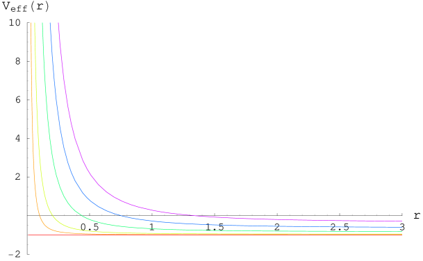
Figure 1: Plot of the effective potential in pure AdS (with $R=1$) for a sample of null geodesics, with $E=1.0$ and $L=0.0,0.1,0.2,0.4,0.6$ and $0.8$

$$V_{eff}=-\left(f(r)\kappa+E^{2}-\frac{f(r)L^{2}}{r^{2}}\right)$$ (9)

Note that the RHS of (8) is zero, and so any part of the effective potential which is positive represents a potential barrier, see Fig.1. The minimum value of r obtained by spacelike and null geodesics incoming from $r=\infty$ is given by the largest solution to $V_{eff}=0$, and is the endpoint (starting point) of the ingoing (outgoing) part of the geodesic. The paths of geodesics can be calculated and plotted numerically using these equations, and for null geodesics in pure AdS, they can also be calculated analytically (see appendix A).

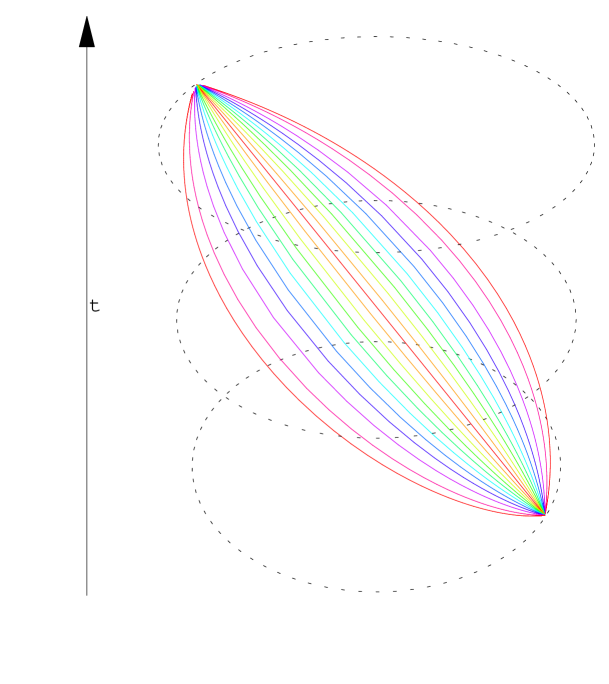
Figure 2: A plot of some null geodesic paths passing through an AdS spacetime, all starting from the same point $t=0$, $\phi=0$ on the boundary at $r=\infty$ (compactified to lie at $\arctan(\infty)=\frac{\pi}{2}$ in the diagram).

For null geodesics in AdS space, their endpoints always lie at the antipodal point no matter what the ratio of angular momentum to the energy. They can be plotted using the compactification given in appendix A, which rescales the boundary at $r=\infty$ to lie on a circle of radius $\pi/2$, see Fig.2.

As mentioned in the introduction, the endpoints of null geodesics correspond to singularities in the set of correlation functions in the field theory lying on the boundary of the spacetime. For the rest of the paper we assume that the endpoint data we use can be generated in such a fashion from the field theory.

3 Asymptotically AdS spacetimes

We can consider a small modification to the pure AdS spacetime described by (1) and (2), by replacing (2) with:

$$f(r)=1+\frac{r^{2}}{R^{2}}-p(r)$$ (10)

where $p(r)$ is an analytic function which behaves as $r^{2}$ for small $r$ and $r^{-2}$ for large $r$, such that the metric is non-singular everywhere.

3.1 Analysing the geodesic endpoints

In this modified spacetime, null geodesic paths do not always end at their antipodal point on the boundary; their final $t$ and $\phi$ coordinates depend on the ratio of the angular momentum ($L$) to the energy ($E$). From a physical point of view this can be thought of as the extra term $p(r)$ representing an attractive modification to the centre of the spacetime, such that the geodesics follow a more curved path through the bulk, and thus “overshoot” the antipodal point. Their extra path length then also accounts for the increase in the time taken to reach the boundary at infinity.

If we consider the set of null geodesics all beginning at the same point, $(t_{0},\phi_{0})$ on the boundary, we can obtain the full spread of endpoints by varying $L/E$ from 0 to 1. Fig.3 shows an example of the geodesic paths in a modified AdS spacetime alongside a plot of their endpoints.

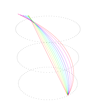
Figure 3: A plot of the null geodesic paths passing through a modified AdS spacetime, all starting from the arbitrary point $t=0$, $\phi=0$ on the boundary and with positive angular momentum. The corresponding full spectrum of null geodesic endpoints for this spacetime is shown on the right.

From this plot of the endpoints, what information about the bulk metric can be recovered? For a geodesic beginning at $(t_{0},\phi_{0})$ and ending at $(t_{1},\phi_{1})$ on the boundary, we have:

$$\int_{t_{0}}^{t_{1}}\,\mathrm{d}t=2\int_{r_{min}}^{\infty}\frac{1}{f(r)\sqrt{1-y^{2}\frac{f(r)}{r^{2}}}}\,\mathrm{d}r$$ (11)

$$\int_{\phi_{0}}^{\phi_{1}}\,\mathrm{d}\phi=2\int_{r_{min}}^{\infty}\frac{y}{r^{2}\sqrt{1-y^{2}\frac{f(r)}{r^{2}}}}\,\mathrm{d}r$$ (12)

where $r_{min}$ is minimum radius obtained by the geodesic, and we have introduced the parameter $y=L/E$ to denote the ratio of the angular momentum to the energy.

We note that for a fixed metric, the final time and angular coordinates will be functions of $y$ only, and so we can write:

$$\int_{t_{0}}^{t_{1}}\,\mathrm{d}t=t_{1}-t_{0}\equiv t(y)$$ (13)

$$\int_{\phi_{0}}^{\phi_{1}}\,\mathrm{d}\phi=\phi_{1}-\phi_{0}\equiv\phi(y)$$ (14)

If we define the function $g(y,r)$ as:

$$g(y,r)=\frac{1}{\sqrt{1-y^{2}\frac{f(r)}{r^{2}}}}$$ (15)

and consider the derivative of (11) and (12) with respect to $y$ we have:

$$\frac{dt(y)}{dy} =2\frac{d}{dy}\left(\int_{r_{min}}^{\infty}\frac{g(y,r)}{f(r)}\,\mathrm{d}r\right)$$ (17)

$$=2y\int_{r_{min}}^{\infty}\frac{\left(g(y,r)\right)^{3}}{r^{2}}\,\mathrm{d}r-\left(\frac{2\,g(y,r)}{f(r)}\right)\Big{|}_{r=r_{min}}\frac{dr_{min}}{dy}$$

and

$$\frac{d\phi(y)}{dy} =2\frac{d}{dy}\left(\int_{r_{min}}^{\infty}\frac{y\,g(y,r)}{r^{2}}\,\mathrm{d}r\right)$$ (19)

$$=2\int_{r_{min}}^{\infty}\frac{\left(g(y,r)\right)^{3}}{r^{2}}\,\mathrm{d}r-\left(\frac{2\,y\,g(y,r)}{r^{2}}\right)\Big{|}_{r=r_{min}}\frac{dr_{min}}{dy}$$

Comparing the integral terms in the two equations above, we see that they are identical upto a factor of $y$. We can then use the fact that at $r=r_{min}$, $y^{2}=\frac{f(r_{min})}{r_{min}^{2}}$ to rewrite the first equation as:

$$\frac{dt(y)}{dy}=2y\int_{r_{min}}^{\infty}\frac{\left(g(y,r)\right)^{3}}{r^{2}}\,\mathrm{d}r-y\left(\frac{2\,y\,g(y,r)}{r^{2}}\right)\Big{|}_{r=r_{min}}\frac{dr_{min}}{dy}$$ (20)

After checking that the divergent piece of the integral cancels with the divergent second term in (20) (see appendix B) we therefore have that:

$$\frac{dt(y)}{dy}=y\,\frac{d\phi(y)}{dy}$$ (21)

which can be rewritten as

$$\frac{dt}{d\phi}=y(\phi)$$ (22)

Thus from the plot of the endpoints, by taking the gradient at each point we are able to obtain the value of $y$ for that geodesic. Note that at no point in this derivation have we used the fact that the spacetime is asymptotically AdS, and it can easily be shown that the result holds for any static, spherically symmetric spacetime (i.e. any metric of the form of (38)). Calculations along these lines are also not restricted to null geodesics, see [14] for similar derivations involving spacelike ones. In the next section we will see how we can further use this to recreate the metric function $f(r)$.

3.2 Reconstructing $f(r)$: Method I

The method involves iteratively recovering $f(r)$ starting from large radius and working down towards $r=0$. We are working in an asymptotically AdS spacetime. This means that as $r\rightarrow\infty$, $f(r)\rightarrow r^{2}/R^{2}+1$; thus we can say that for $r\geq r_{n}$ for some $r_{n}$ which can be arbitrarily large, $f(r)\approx r^{2}/R^{2}+1$. We set the AdS radius ($R$) to one, and by considering large enough $y=y_{n}$ such that the minimum radius, $r_{min}$, corresponds to $r_{n}$, (11) becomes (setting the initial time, $t_{0}$, to be zero):

$$t_{n}=\int_{0}^{t_{n}}\,\mathrm{d}t =2\int_{r_{n}}^{\infty}\frac{g(y_{n},r)}{f(r)}\,\mathrm{d}r$$ (24)

$$\approx 2\int_{r_{n}}^{\infty}\frac{1}{(r^{2}+1)\sqrt{1-y_{n}^{2}\frac{r^{2}+1}{r^{2}}}}\,\mathrm{d}r=\pi$$

as we would expect, as geodesics remaining far from the centre of the space would not “see” the modification and thus behave as in pure AdS. In this case we can solve the equation for the minimum radius:

$$y_{n}^{2}=\frac{r_{n}^{2}}{f(r_{n})}=\frac{r_{n}^{2}}{r_{n}^{2}+1}$$ (25)

to get $r_{n}$ in terms of $y_{n}$, which is determined from the geodesic endpoints. Thus we can determine $r_{n}$ (and hence $f(r_{n})=r_{n}^{2}+1$).

If we now consider a geodesic with slightly lower ratio of angular momentum to energy, say with $y_{n-1}=y_{n}-\epsilon$, where $\epsilon>0$, we have the equation:

$$t_{n-1}=2\int_{r_{n-1}}^{\infty}\frac{g(y_{n-1},r)}{f(r)}\,\mathrm{d}r$$ (26)

which can be split up as follows (noting that $r_{n-1}<r_{n}$):

$$t_{n-1}=2\int_{r_{n-1}}^{r_{n}}\frac{g(y_{n-1},r)}{f(r)}\,\mathrm{d}r+2\int_{r_{n}}^{\infty}\frac{g(y_{n-1},r)}{f(r)}\,\mathrm{d}r$$ (27)

The second integral can be evaluated by setting $f(r)=r^{2}+1$ as in (24), and we have

$$2\int_{r_{n}}^{\infty}\frac{g(y_{n-1},r)}{f(r)}\,\mathrm{d}r=\pi-2\arctan{\left(\sqrt{\left(1-y_{n-1}^{2}\right)r_{n}^{2}-y_{n-1}^{2}}\,\right)}$$ (28)

We can approximate the first integral by taking a Laurent expansion about the point $r_{n-1}$. This gives, to lowest order:

$$\int_{r_{n-1}}^{r_{n}}\frac{g(y_{n-1},r)}{f(r)}\,\mathrm{d}r \approx\int_{r_{n-1}}^{r_{n}}\frac{(r-r_{n-1})^{-1/2}}{f(r_{n-1})\sqrt{\frac{2}{r_{n-1}}-\frac{f^{\prime}(r_{n-1})}{f(r_{n-1})}}}\,\mathrm{d}r$$ (30)

$$=\frac{2\sqrt{r_{n}-r_{n-1}}}{f(r_{n-1})\sqrt{\frac{2}{r_{n-1}}-\frac{f^{\prime}(r_{n-1})}{f(r_{n-1})}}}$$

where we have used that $y_{n-1}^{2}=r_{n-1}^{2}/f(r_{n-1})$ and integrated. This can be simplified further by writing:

$$f^{\prime}(r_{n-1})\approx\frac{f(r_{n})-f(r_{n-1})}{r_{n}-r_{n-1}}$$ (31)

Thus we have:

$$t_{n-1}\approx\frac{4(r_{n}-r_{n-1})}{f(r_{n-1})\sqrt{\frac{2r_{n}}{r_{n-1}}-\frac{f(r_{n})}{f(r_{n-1})}-1}}+\pi-2\arctan{\left(\sqrt{\left(1-y_{n-1}^{2}\right)r_{n}^{2}-y_{n-1}^{2}}\,\right)}$$ (32)

which can be used in conjunction with $y_{n-1}^{2}=r_{n-1}^{2}/f(r_{n-1})$ to calculate $r_{n-1}$ and $f(r_{n-1})$, as we know $t_{n-1}$ and $y_{n-1}$ from the geodesic endpoints, and $r_{n}$ and $f(r_{n})$ have already been calculated.

For general $t_{n-i}$ we split the integral into several pieces; the two “end” integrals, which we evaluate as in (28) and (30), and a series of integrals in the middle which can be evaluated using the trapezium rule or similar (see Fig.4). The formula for general $t_{n-i}$ is then given by (for $i\geq 2$):

$$t_{n-i} =2\int_{r_{n-i}}^{\infty}\frac{g(y_{n-i},r)}{f(r)}\,\mathrm{d}r$$ (34)

$$\approx A_{n-i}+B_{n-i}+C_{n-i}$$

where

$$A_{n-i}=\frac{4\,(r_{n-i+1}-r_{n-i})}{f(r_{n-i})\sqrt{\frac{2r_{n-i+1}}{r_{n-i}}-\frac{f(r_{n-i+1})}{f(r_{n-i})}-1}}$$ (35)

$$B_{n-i}=\sum_{j=1}^{i-1}\left(r_{n-j+1}-r_{n-j}\right)\left(\frac{g(y_{n-i},r_{n-j+1})}{f(r_{n-j+1})}+\frac{g(y_{n-i},r_{n-j})}{f(r_{n-j})}\right)$$ (36)

$$C_{n-i}=\pi-2\arctan{\left(\sqrt{\left(1-y_{n-i}^{2}\right)r_{n}^{2}-y_{n-i}^{2}}\,\right)}$$ (37)

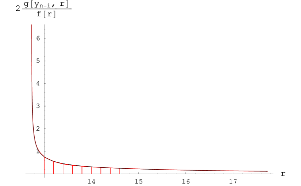
Figure 4: A plot showing how the integrand of (34), is split up into two end curves and a number of trapeziums in order for the integral to be well approximated. The actual curve is shown in black, with the approximations in red.

For a spacetime of the form of (10) with monotonic effective potential, we can use the above to recover the function $f(r)$ down to $r=0$. See section 5 for examples.

3.3 More general spacetimes

So far we have restricted ourselves to considering metrics of the form of (1), however, we can look to extend this further by considering the most general static, spherically symmetric spacetimes, given by metrics of the form:

$$ds^{2}=-f(r)dt^{2}+h(r)dr^{2}+r^{2}d\Omega_{3}^{2}$$ (38)

where the $dr^{2}$ coefficient is allowed to be different to the $dt^{2}$ coefficient. Equations (3) and (4) for the geodesics remain unchanged, and the third is now given by:

$$\dot{r}^{2}-\left(\frac{\kappa}{h(r)}+\frac{E^{2}}{f(r)h(r)}-\frac{L^{2}}{h(r)r^{2}}\right)=0$$ (39)

where $\kappa=0$ for the null case. We can combine the equations together as before to give the integral equations:

$$\int_{t_{0}}^{t_{1}}\,\mathrm{d}t=2\int_{r_{0}}^{\infty}\frac{1}{\frac{f(r)}{\sqrt{h(r)}}\sqrt{\frac{1}{f(r)}-\frac{y^{2}}{r^{2}}}}\,\mathrm{d}r$$ (40)

$$\int_{\phi_{0}}^{\phi_{1}}\,\mathrm{d}\phi=2\int_{r_{0}}^{\infty}\frac{y}{\frac{r^{2}}{\sqrt{h(r)}}\sqrt{\frac{1}{f(r)}-\frac{y^{2}}{r^{2}}}}\,\mathrm{d}r$$ (41)

The question now is whether we can use the two equations above along with the expression $y^{2}=r_{0}^{2}/f(r_{0})$ relating the parameter $y$ to the minimum radius to recover both $f(r)$ and $h(r)$ and thus reconstruct the bulk metric from the endpoints. This initially appears possible as we haven’t explicitly used our expression for $\phi$, (41), in our method of the previous section. However, our observation that the gradient of the endpoints is given by the angular momentum (22) suggests that we don’t have three linearly independent relations. Attempting to continue as before, by approximating the spacetime as pure AdS at some large radius and working inwards, the degeneracy soon becomes apparent (see appendix C), and we are unable to recover bulk metric information in these more general spacetimes (unless we a priori know the relationship between $h(r)$ and $f(r)$).

3.4 Reconstructing $f(r)$: Method II

There is an alternative method for reconstructing $f(r)$ in a spacetime of the form of (1) which makes the degeneracy of the expressions for $t$ and $\phi$ more apparent. If we start from expression (21) and integrate over $y$ we get:

$$\int^{t}\,\mathrm{d}t^{\prime}=\int y\frac{d\phi}{dy}\,\mathrm{d}y$$ (42)

which can be integrated by parts:

$$t(y)=y\,\phi(y)-\int\phi\,\mathrm{d}y$$ (43)

and then rewritten using the expression for $\phi$ from (12):

$$t(y)=y\,\phi(y)-\int\int_{r_{min}}^{\infty}\frac{2y}{r^{2}\sqrt{1-y^{2}\frac{f(r)}{r^{2}}}}\,\mathrm{d}r\,\mathrm{d}y$$ (44)

We can now reverse the order of integration, and as the function $f(r)$ has no dependence on $y$, integrate over $y$:

$$t(y)=y\,\phi(y)+\int_{r_{min}}^{\infty}\frac{2}{f(r)}\sqrt{1-y^{2}\frac{f(r)}{r^{2}}}\,\mathrm{d}r$$ (45)

Taking the initial conditions to be $(\phi_{0},t_{0})=(0,0)$, we can say that for any endpoint $(\phi_{j},t_{j})$ on the boundary,

$$t_{j}-\frac{dt}{d\phi}\Big{|}_{(\phi_{j},t_{j})}\phi_{j}=\int_{r_{j}}^{\infty}\frac{2}{f(r)\,g(y_{j},r)}\,\mathrm{d}r$$ (46)

where we have renamed the minimum $r$ as $r_{j}$ and used our definition for $g(y,r)$ from before. This, coupled with the equation for the minimum $r$,

$$y_{j}^{2}=\frac{r_{j}^{2}}{f(r_{j})}$$ (47)

allows the metric function $f(r)$ to be fully reconstructed from the plot of the endpoints, using a method of approximating the integral similar to that in section 3.2.

4 Analysing the two methods

Whilst the previous methods both in principle allow the bulk metric to be fully recovered (from $f(r_{n})$ down to $f(0)$, with $r_{n}$ arbitrarily large), there are a number of factors to take into account when performing the reconstruction in practice, in order to obtain a balance between accuracy and computational effort.

Consider a setup where we divide the range of $y$ into $N+1$ equal segments, with $y_{0}=0$ and $y_{N+1}=1$, so that we have $N+1$ steps in the process of recovering $f(r)$ (Note that the first step in the iteration uses $y_{N}$ rather than $y_{N+1}$, as we want the first minimum radius to be finite).

There are a number of issues with recovering $f(r)$ in this scenario. We firstly observe that splitting $y$ up into equal segments means that the minimum radii will not be equally separated; there will be a greater number of low radius points (due to the shape of $V_{eff}$). This initially appears helpful, as we expect most of the bulk metric’s deviation from pure AdS to be localised close to the centre, and so a greater number of data points in this region should improve our estimate of $f(r)$.

However, as both methods for recovering $f(r)$ involve approximating integrals over $r$, accuracy is only maintained if the step size is kept relatively small for all $r$; whilst starting with $y_{N}$ as close to one as possible allows $f(r)$ to be recovered from as large a radius as possible (as higher $y_{N}$ means higher $r_{N}$), this also means the first few steps in $r$ will be unacceptably large. This can be countered by ensuring the number of steps is appropriately large, however, this will then result in a longer computational time. For example, in the asymptotically AdS spacetime with $f(r)$ given by

$$f(r)=1+r^{2}-\frac{4r^{2}}{(r^{2}+1)(r^{2}+8)}$$ (48)

if use a step size in y of $0.0005$ and take the initial $y_{N}$ to be $0.9995$, the corresponding minimum radius $r_{N}\approx 31.5$. The minimum radius corresponding to $y_{N-1}=0.999$ is only $r_{N-1}\approx 22.3$ however, and such a large jump in the radius causes problems with using our approximation of the form of (32). Whilst the original Laurent expansion of (30) is still fairly accurate over this distance, our approximation of the gradient by

$$f^{\prime}(r_{n-i})=\frac{f(r_{n-i+1})-f(r_{n-i})}{r_{n-i+1}-r_{n-i}}$$ (49)

is not. For the example above, the actual value of $f^{\prime}(r)$ at $r=22.3$ is 44.5, whereas the value given by (49) is 53.8; a large discrepancy.

We can still split the $y_{n}$ linearly (in order to keep the majority of the points at low radii), however, we choose the initial $y_{N}$ to be be slightly lower. This enables our first step in the radius to be kept small. In our example of (48), if we choose $y_{N}=0.9985$ and keep the step size at $0.0005$, we find that $r_{N}-r_{N-1}\approx 2.5$ which whilst still quite large, is much more acceptable than the value of $9.2$ we had previously. Table 1 shows how this discrepancy in the gradient affects the extraction of $f(r)$ by the method of section 3.2 for the example of (48); it is worth noting at this stage that even with the lower choice of starting $y$ the recovered estimate for $f(r)$ is still quite poor with a step size of $0.0005$. This is important because although we could lower $y_{N}$ even further, we must keep our initial radius reasonably large; if we choose $y_{N}$ to be too low, we risk having $r_{N}$ being too small, such that our assumption that the spacetime there is approximately that of pure AdS is no longer valid. We can keep our choice of $y_{N}$ high by reducing the step size (as in the lower half of Table 1), but at the expense of additional computational time (For more details on the numerical extraction see the examples in the next section).

Initial y	Step size	$\alpha$ (4)	$\beta$ (1)	$\gamma$ (8)
0.9995	0.0005	0.778	0.971	0.971
0.9985	0.0005	1.39	1.52	1.52
0.9995	0.00005	2.37	2.24	2.24
0.9985	0.00005	3.42	1.13	6.18

Table 1: Comparing the accuracy of using two different values for $y_{N}$ to recover the bulk metric information. The actual values for $\alpha$, $\beta$ and $\gamma$, which correspond to the three numerical factors in (48) (and are properly defined in (53)), are given in brackets. More details on how these estimates were generated is given in section 5.

There is, however, another problem with numerically reconstructing $f(r)$ using the approximation of the gradient by (49). If we examine the form of the term containing $f^{\prime}(r)$, namely the $A_{n-i}$ in (34), whose equivalent in method II is:

$$A_{n-i}=\frac{4}{3}\frac{(r_{n-i+1}-r_{n-i})}{f(r_{n-i})}\sqrt{\frac{2}{r_{n-i}}-\frac{f^{\prime}(r_{n-i})}{f(r_{n-i})}}$$ (50)

we note that the $f^{\prime}(r)$ appears with a negative sign inside the square root. As our approximation of $f^{\prime}(r)$ by (49) is in general an overestimation of the gradient, as for large $r$, $f(r)\propto r^{2}+1$, when solving for $r_{n-i}$ and $f(r_{n-i})$ the term under the square root can become negative, leading to the estimates being imaginary. This can occur even if the overestimation is small.

There are a number of possible ways in which to resolve this problem. We can firstly consider a different approximation of the gradient to the one given in (49); the over-estimation can be avoided by using an expression such as

$$f^{\prime}(r_{n-i})=\frac{1}{2}\Big{(}\frac{f(r_{n-i+1})-f(r_{n-i})}{r_{n-i+1}-r_{n-i}}+\frac{f(r_{n-i})-f(r_{n-i-1})}{r_{n-i}-r_{n-i-1}}\Big{)}$$ (51)

which takes the average of the two nearest linear tangents to the curve. Inserting this expression into either of our iterative methods for recovering $f(r)$, however, immediately raises a new problem from a computational point of view; we now cannot recover a value for $r_{n-i}$ and $f(r_{n-i})$ at each step, as the $n-i$ term now also depends on the subsequent term, $n-i-1$, as well as the previous. We now have to determine all the equations for the various steps and solve them together at the end to recover $f(r)$. This is a much more complicated operation than numerically solving at each step, and leads to a considerable increase in the computational effort required to reconstruct the metric function.

Another approach is to take a higher order series expansion around the minimum radius in our approximation of the integral, however we then need an expression for the second (or higher) derivative of $f(r)$, which leads to an escalation of the problems mentioned above; either the overestimation caused by only using approximations involving larger $r$ terms upsets the recovery of $r_{n-i}$ and $f(r_{n-i})$, or we need to wait and solve all the equations at the end of all the steps, again greatly increasing the computational effort required.

The gradient of $f(r)$ appears in the integral of (34) because of the Laurent expansion we have used in its approximation; in method II, however, we can use a different approximation which avoids this.

Figure 5: A plot showing an example curve (the integrand of (46)) to be approximated in method II. The leftmost part of the curve is initially a vertical parabola.

Fig.5 shows a plot of a typical curve we are trying to approximate. The crucial difference between this type of curve and that of Fig.4 is the behaviour at the minimum radius, which is due to the positioning of the $g(y,r)$ term in equations (34) and (46). That $g(y,r)$ appears in the denominator of (46) rather than the numerator results in the curve of Fig.5 having an infinite gradient at the minimum radius. We can then describe the leftmost part of the curve as following a vertical parabolic path. Thus instead of using a Laurent approximation at this point, we can make a geometric one and say that:

$$A_{n-i}=\frac{4}{3}\frac{(r_{n-i+1}-r_{n-i})}{f(r_{n-i+1})}\sqrt{1-\frac{y_{n-i}^{2}}{y_{n-i+1}^{2}}}$$ (52)

where we have used that the area under a parabola is $2/3$ the width multiplied by the height. The gradient of the curve will always be infinite at the minimum radius, and as the other terms ($B_{n-i}$ and $C_{n-i}$) do not depend on $f^{\prime}(r)$, we avoid the need for an approximation to the gradient of the form of (49). Importantly, we also avoid any increase in the computational effort required to recover $f(r)$. It is also worth noting that there is no similar geometric argument for such an approximation to be applied in the original method of section 3.2. For similar step size this modification leads to a considerably more accurate estimation of $f(r)$ from the endpoints, as we shall see in the next section, where we use both methods to reconstruct $f(r)$ in two different cases.

5 Examples

Consider a small deviation from pure AdS, such as the spacetime with metric function $f(r)$ as in (48). Choosing our initial value of $y$ to be $y_{N}=0.9985$ (for the reasons of the previous section), we investigate the ability of the two methods to extract the bulk information. Fig.6 shows our approximations of $f(r)$ generated using method I for a range of different step sizes.

For this first example, the top set of curves in Fig.6 suggest that we are easily able to extract the bulk metric using any of the step sizes, as they all appear to lie very close to the actual function $f(r)$. However, this is somewhat misleading, as we shall see. In order to more closely examine the accuracy of the recovered bulk data, we use a non-linear fit of the form:

$$f(r)=1+r^{2}-\frac{\alpha\,r^{2}}{(r^{2}+\beta)(r^{2}+\gamma)}$$ (53)

to obtain values for $\alpha$, $\beta$ and $\gamma$ for each estimate, and the results are presented in Table 2. As we mentioned above, looking at the top plot of Fig.6, all of the approximations seem very close to the original function, however, Table 2 shows this not to be the case. Until we go to a very small step size, we are unable to accurately extract what one might consider the important metric information; if the modification of the spacetime caused by the extra term in (48) was to correspond to some physical phenomenon, we might expect its “mass” and “extent” to be related to the quantities $\alpha$, and $\beta$ and $\gamma$ respectively. Whilst the best fits we obtain are converging to the correct values as we take the step size smaller, we are already calculating a significant number of terms to generate these estimates.

Initial y	Step size	$\alpha$ (4)	$\beta$ (1)	$\gamma$ (8)
0.9985	0.002	0.371	0.530	0.530
0.9985	0.001	0.797	0.995	0.995
0.9985	0.0005	1.39	1.52	1.52
0.9985	0.0002	2.18	2.11	2.11
0.9985	0.0001	2.74	1.47	3.92
0.9985	0.00005	3.42	1.13	6.18
0.9985	0.00002	3.80	1.11	7.20

Table 2: Best fit values (to 3 s.f.) for $\alpha$, $\beta$ and $\gamma$ for data generated using method I, with the actual values indicated in brackets. Only in the lower half of the table do the estimates for the three unknowns really start to converge to the correct values.

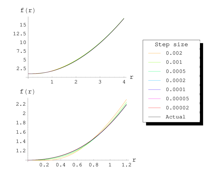
Figure 6: Plots showing the various estimates for $f(r)$ given in Table 2 (i.e. produced using method I), compared to the actual metric function $f(r)$ from (48). Whilst all the estimates seem good fits over a large radius (top figure), closer consideration of the curves highlights their differences (bottom figure), which lead to the inaccurate values calculated for $\alpha$, $\beta$ and $\gamma$ from the larger step size estimates.

Initial y	Step size	$\alpha$ (4)	$\beta$ (1)	$\gamma$ (8)
0.9985	0.002	1.61	2.01	2.01
0.9985	0.001	3.34	1.16	6.01
0.9985	0.0005	3.92	1.01	7.77
0.9985	0.0002	3.99	1.00	7.97
0.9985	0.0001	4.00	1.00	8.00

Table 3: Best fit values (to 3 s.f.) for $\alpha$, $\beta$ and $\gamma$ for data generated using method II, with the actual values indicated in brackets. Using the alternative method, we are able to pick out rough values for the three unknowns as early as with a step size of $0.001$, and by a step size of $0.0001$ the estimates have converged to the correct values (to 3 s.f.).

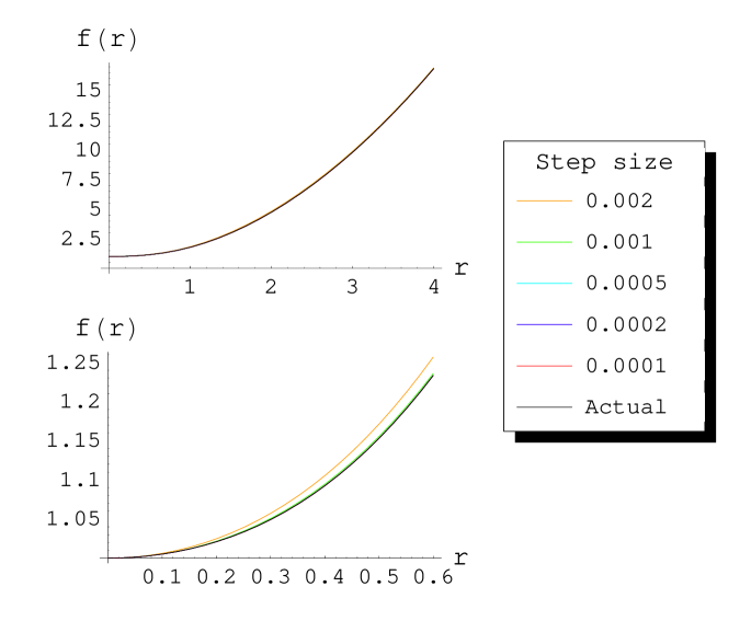
Figure 7: Plots showing the various estimates for $f(r)$ given in Table 3, compared to the actual metric function $f(r)$ from (48). Using method II for producing the estimates has resulted in much closer fits, both over a large radius (top figure), and at smaller scales (bottom figure). This is reflected in the highly accurate values of $\alpha$, $\beta$ and $\gamma$ determined from the all but the largest step size estimates.

If we compare this to the fits we obtain using the data calculated via method II, with the modification to the $A_{n-i}$ terms given in (52), we see a notable difference in the results. The estimates again all look good when plotted with the actual function $f(r)$, as we see in Fig.7, however, as the bottom plot shows, this accuracy is now maintained at smaller scales. Table 3 shows the new values for $\alpha$, $\beta$ and $\gamma$ for each step size, obtained using the same non-linear fit, (53), as before.

Comparing these estimates with those in Table 2, we see that the recovered values for $\alpha$, $\beta$ and $\gamma$ are far more accurate using this alternative method, for each choice of step size. We now have a very good fit to the actual values of 4,1 and 8 in (48) obtained using a relatively low number of steps, and thus relatively quickly. Indeed, we see that to obtain the same degree of accuracy using method I we need to use step sizes which are more than twenty five times smaller, which (assuming a standard computational time per step) would therefore take at least twenty five times longer to compute. Thus using the modified second method offers a significant improvement over the original.

Can we use the methods to recover a more complicated $f(r)$? If we consider a spacetime similar to that in (48), but which is further modified at low $r$ by an extra term:

$$f(r)=1+r^{2}-\frac{4r^{2}}{(r^{2}+1)(r^{2}+8)}+\frac{3r\sin(2r)}{r^{4}+1}$$ (54)

we can use both methods to generate estimates for $f(r)$, and using a non-linear fit of the form of:

$$f(r)=1+r^{2}-\frac{\alpha\,r^{2}}{(r^{2}+\beta)(r^{2}+\gamma)}+\frac{\chi r\sin(\eta r)}{r^{4}+\lambda}$$ (55)

we can judge the accuracy of the estimate against (54). Using the same starting value for $y$ and the same step sizes as before, we obtain the results shown in tables 4 and 5, and figures 8 and 9.

Initial y	Step size	$\alpha$ (4)	$\beta$ (1)	$\gamma$ (8)	$\chi$ (3)	$\eta$ (2)	$\lambda$ (1)
0.9985	0.002	-1380	133	133	2.60	2.20	1.20
0.9985	0.001	0.0824	0.426	0.426	2.69	2.12	1.04
0.9985	0.0005	0.790	0.880	0.880	2.96	2.03	0.981
0.9985	0.0002	1.69	1.25	1.25	3.06	1.95	0.940
0.9985	0.0001	2.23	1.62	1.62	3.05	1.94	0.946
0.9985	0.00005	2.87	2.39	2.39	3.00	1.97	0.985
0.9985	0.00002	3.68	1.31	6.50	3.09	2.00	1.04

Table 4: Best fit values (to 3 s.f.) for $\alpha$, $\beta$, $\gamma$, $\chi$, $\eta$ and $\lambda$ for data generated using method I, with the actual values indicated in brackets. In this more complicated modification to AdS, the presence of the sine term masks the finer structure and prevents the original method from converging towards the correct values of $\beta$ and $\gamma$ until our smallest choice of step size.

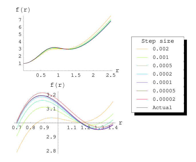
Figure 8: Plots showing the various estimates for $f(r)$ given in Table 4 (i.e. produced using method I), compared to the actual metric function $f(r)$ from (54). The convergence of the estimates to the actual curve can be seen in both plots, and whilst the values obtained for $\chi$, $\eta$ and $\lambda$ are reasonably good for all step sizes, only upon using the smallest step size do we start to pick out the $\alpha$, $\beta$ and $\gamma$ values. This is why, in the lower figure, the red curve representing the final estimate appears to be a worse fit to the actual curve than some of the others; the range of $r$ shown highlights the accuracy of the $\chi$, $\eta$ and $\lambda$ values rather than the $\alpha$, $\beta$ and $\gamma$ ones.

Initial y	Step size	$\alpha$ (4)	$\beta$ (1)	$\gamma$ (8)	$\chi$ (3)	$\eta$ (2)	$\lambda$ (1)
0.9985	0.002	1.17	1.46	1.46	3.47	1.94	1.12
0.9985	0.001	2.90	2.52	2.52	3.03	1.97	0.998
0.9985	0.0005	3.85	1.06	7.38	3.00	2.00	1.00
0.9985	0.0002	3.98	1.01	7.93	3.00	2.00	1.00
0.9985	0.0001	4.00	1.00	7.99	3.00	2.00	1.00
0.9985	0.00005	4.00	1.00	8.00	3.00	2.00	1.00

Table 5: Best fit values (to 3 s.f.) for $\alpha$, $\beta$, $\gamma$, $\chi$, $\eta$ and $\lambda$ for data generated using method II, with the actual values indicated in brackets. Once again, the alternative method proves much more adept at accurately estimating the unknowns, and converges to the correct values almost immediately.

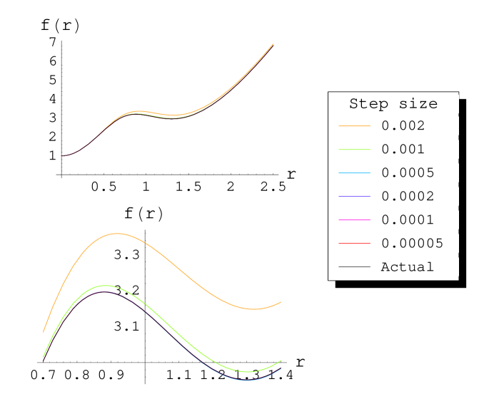
Figure 9: Plots showing the various estimates for $f(r)$ given in Table 5 (i.e. produced using method II), compared to the actual metric function $f(r)$ from (54). Only the estimates generated using the largest two step sizes are visibly distinguishable from the actual curve, as the the values of $\alpha$, $\beta$, $\gamma$, $\chi$, $\eta$ and $\lambda$ are all quickly picked out using this alternative method.

Once again we see that the second method produces a much better estimate of $f(r)$ than the first; the difference in the accuracy is again significant. What is also noticeable in this slightly more complicated example is that the presence of a more prominent feature in the metric function (in this case the small oscillation from the sine term) can obscure the finer details of the spacetime. This is most obvious in the results from using method I (see Table 4, where we can clearly see that whilst the numerical factors corresponding to the sine term ($\chi$, $\eta$ and $\lambda$) are easily determined even at a large step size, it then requires a smaller step size to pick out the $\alpha$, $\beta$ and $\gamma$ values than it did in the first example.

Whilst the second example has shown that the methods can be used for $f(r)$ which have a significant deviation from pure AdS near the centre, there remain problems in applying the methods in certain circumstances, which are examined in the next section.

6 Limitations

There are limitations in recovering $f(r)$ all the way down to $r=0$ in the cases where the metric is non-singular but does not give a monotonic effective potential for the null geodesics, and also when there is a curvature singularity at $r=0$.

6.1 Metrics with a non-monotonic effective potential

There is a problem with the method for reconstructing $f(r)$ if the metric is such that for some critical value of the angular momentum, the null geodesics can go into an unstable orbit (assuming fixed energy). This is indicated on the endpoint plot by the $\phi$ coordinate heading off to infinity, and the presence of a jump in the time taken by the geodesics with $L<L_{crit}$ compared with those with $L>L_{crit}$, see Fig.10 for an example.

The reason for these unstable orbits is because the effective potential for the metric isn’t monotonic; the orbits occur when the greatest radius ($r_{p}$ say) for which $dV/dr=0$ corresponds with that for which $V=0$, see Fig.11. This non-monotonicity also explains the time delay for those geodesics with angular momentum lower than $L_{crit}$, indicated by the gap between the asymptotes in Fig.10: those with slightly lower $L$ have an effective potential of the form shown as the dashed blue curve in Fig.11, and travel down to minimum radius $r_{p-1}$, whereas those with $L\geq L_{crit}$ have minimum radius greater than or equal to $r_{p}$, indicated by the dashed red curve. The extra (non-negligible) distance $r_{p}-r_{p-1}$ travelled by the geodesics results in the time delay seen in the endpoints.

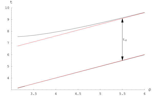
Figure 10: Plot of the endpoints of null geodesics which all begin from the same point on the boundary and pass through an AdS-like space time with non-monotonic $V_{eff}$. The red lines indicate the limits to which the black curves tend as $L\rightarrow L_{crit}$

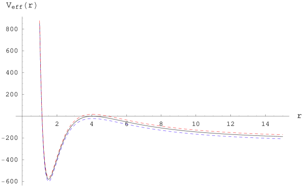
Figure 11: Plot of the effective potential for three null geodesics: one with the critical angular momentum, $L_{crit}$ (the solid black curve), one with $L<L_{crit}$ (the lowest curve, dashed blue), and one with $L>L_{crit}$ (top curve, dashed red).

We thus have the situation where we have no geodesics with minimum radius $r_{q}$, where $r_{p-1}<r_{q}<r_{p}$, and this is where our iterative methods break down. Although we can begin by using one of the methods from earlier to recover $f(r)$ down to $r=r_{p}$, which corresponds to using the endpoints in the “lower branch” of Fig.10, we cannot continue past this point. Using method I, say, the final term of the iteration will be:

$$t_{p}=2\int_{r_{p}}^{\infty}\frac{1}{f(r)\sqrt{1-y_{p}^{2}\frac{f(r)}{r^{2}}}}\,\mathrm{d}r\approx A_{p}+B_{p}+C_{p}$$ (56)

with $A_{p}$, $B_{p}$ and $C_{p}$ defined as in section 3.2. As the next term would involve an integration over the range $r_{p-1}$ to $r_{p}$, which cannot necessarily be taken to be small, it cannot be well approximated by the methods we have used previously.

The gap between the upper and lower branches of Fig.10 tends to a constant time delay, $t_{d}$, as $\phi\rightarrow\infty$, and it is this which corresponds to the integral we are unable to well approximate:

$$t_{d}=2\int_{r_{p-1}}^{r_{p}}\frac{1}{f(r)\sqrt{1-y_{p-1}^{2}\frac{f(r)}{r^{2}}}}\,\mathrm{d}r$$ (57)

where we note that in the limit $\phi\rightarrow\infty$ we have that $y_{p-1}=y_{p}$.

We are left with the situation where we do not have enough information to carry on recovering $f(r)$ past the rightmost maximum in the effective potential; there is no approximation we could attempt to make without already knowing more about the form of $V_{eff}$. Although we have the extra endpoint data (i.e. the top branch of 10), we are unable to use it to extract f(r).

Having discovered this apparent limitation in the extraction of the bulk metric, we should ask ourselves how often we would expect to find metrics which give non-monotonic effective potentials for the null geodesics. In other words, how often do we find spacetimes which allow stable orbits of light rays? Whilst it is very easy to construct metrics by hand which allow this, in physical systems circular orbits of light rays are a rarity. Indeed, recent work by Hubeny et al., [23], indicates that for metrics corresponding to a gas of radiation in AdS, it is impossible for circular null geodesics to occur.

Admittedly our restrictive case of metrics of the form of (1) are unrealistic, as any metric of this form necessarily has opposite sign pressure and energy density components of the stress tensor, and as our methods currently do not work in the more general metrics, (38), this is merely an observation.

One scenario in which null geodesics can go into circular orbits is around black holes, and we now conclude the current section by considering such an example.

6.2 Metrics containing a singularity

We ask what information can be retrieved if the metric contains a singularity at its centre, for example Schwarzschild-AdS. We again cannot recover the entirety of $f(r)$, as the geodesics which pass behind the horizon will not return out to the boundary. Thus whilst in the non-monotonic case we had extra information (the top branch of Fig.10) available but no way to get past the jump in the minimum radii of the geodesics, here we only have a reduced spectrum of endpoints from which to recover $f(r)$.

The endpoints we do obtain are those with angular momentum above some critical value, and so we can use the above iterative method to recover $f(r)$ down to a certain critical radius (which will be greater than the horizon radius). However, any null geodesics which pass behind the horizon will always terminate at the singularity, and so we are unable to obtain any further information using our iterative method.

For an example we consider five dimensional Schwarzschild-AdS, in which the metric function $f(r)$ is given by:

$$f(r)=1+\frac{r^{2}}{R^{2}}-\frac{r_{h}^{2}}{r^{2}}\left(\frac{r_{h}^{2}}{R^{2}}+1\right)$$ (58)

where $R$ is again the AdS radius, and $r_{h}$ is the horizon radius. We set $R=1$ as usual, and note that the effective potential for null geodesics is given by:

$$V_{eff}=\left(1+\frac{r^{2}}{R^{2}}-\frac{r_{h}^{2}}{r^{2}}\left(\frac{r_{h}^{2}}{R^{2}}+1\right)\right)\frac{L^{2}}{r^{2}}-E^{2}$$ (59)

For a null geodesic to avoid hitting the singularity at $r=0$, we require $V_{eff}=0$ for some $r>r_{h}$. The lowest $L$ for which this will happen will be when the gradient of $V_{eff}$ is also zero. Differentiating (59) with respect to $r$, and setting equal to zero gives

$$\frac{2L^{2}}{r^{5}}\left(2\left(r_{h}^{2}+r_{h}^{4}\right)-r^{2}\right)=0$$ (60)

which is equal to zero when $r=\sqrt{2}\sqrt{r_{h}^{2}+r_{h}^{4}}$. Thus for the case where $r_{h}=1$ say, the minimum $r$ which can be probed by the null geodesics is $r=2$, and hence we can obtain information about the metric function $f(r)$ from $r=\infty$ down to $r=2$.

7 Discussion

We have seen that the endpoints of null geodesics can be used to recover information about the bulk in asymptotically AdS spacetimes. By varying the ratio of angular momentum to energy of the geodesics we are able to systematically probe to different radii, and this, combined with the appropriate AdS boundary conditions, allows us to reconstruct the metric. What is perhaps quite surprising is that this local, geometric information about the spacetime can be completely recovered in certain scenarios; in a metric of the form of (1), as long as the effective potential for the null geodesics is monotonic, we are able to completely recover the function $f(r)$. Whilst this is of course due to the fact that we have severely restricted our spacetime in such a scenario, to ensure that the amount of information we require is contained within the bi-local spectrum of endpoints, it is still impressive that the recovery process itself is so simple. Its simplicity lies in the remarkable nature of our expression for the gradient of the endpoints of null geodesics (22); to have that the relative angular momentum of the geodesic corresponds to the endpoint in such an accessible fashion is astounding, and forms the basis of our ability to reconstruct the bulk.

Focusing on the cases with a monotonic $V_{eff}$, we developed two different methods for carrying out the recovery of the bulk information, both of which involved iteratively reconstructing $f(r)$ from large $r$ down to the centre. In the process of actually using these methods to numerically extract the bulk information, we made several refinements to increase their efficiency, the most important of which involved our approximation of the gradient of $f(r)$. In both our original methods, we were consistently overestimating $f^{\prime}(r)$, a problem that was significantly affecting their accuracy, unless we kept the iterative step size very small. Whilst we suggested a number of ways of resolving this problem, all made the process of recovering $f(r)$ considerably more complex to implement, thus requiring a great deal of extra computational effort. Given that one of the main aims in this work was to produce a practical method for the recovery of the metric information, these resolutions were not acceptable. Rather than investigating further methods of approximating $f^{\prime}(r)$, we looked at the question of why we needed an approximation to the gradient of $f(r)$ at all, as $f^{\prime}(r)$ does not appear anywhere in our original geodesic equations.

The solution lay in finding an alternative to the Laurent series we were using to approximate the section of the geodesic path close to its minimum radius. Whilst this had been the natural approximation to use in our first method, there was a simpler one we could apply in the second, which stemmed from a crucial difference in the type of curve we were trying to approximate. In method I, the curve in question is infinite at the minimum radius, because the $g(y,r)$ term (see (15)) appears in the numerator of (34). In method II, on the other hand, the $g(y,r)$ term appears in the denominator of the relevant equation, (46), which results in the curve being zero with an infinite gradient. This allowed us to approximate the curve geometrically by a vertical parabola, and thus the integral by the corresponding parabolic area formula. This modification enabled us to estimate $f(r)$ far more efficiently, as it removed any reference to $f^{\prime}(r)$. It also greatly improved the ability of the iterative process to extract what one might consider the important metric information: the numeric values relating to the “mass” and “extent” of whatever physical phenomenon was causing the deviation from pure AdS.

We concluded the project by considering two alternative scenarios: where the effective potential was non-monotonic, and where the metric contained a singularity at the centre. In each case, we were only able to recover $f(r)$ down to a certain critical radius, corresponding to a local maximum of $V_{eff}$ (see fig.11). We were unable to continue the process of recovering $f(r)$ any further as, in the non-singular case, there is a non-negligible “jump” in the minimum radii of the geodesics, due to the shape of the effective potential, which we cannot well approximate. Thus although we have additional endpoint data, we are unable to use it to extract more of the bulk information; we do, however, note that in physical situations, which is where we would eventually hope to apply these techniques, we do not often encounter such metrics (i.e. spacetimes in which light rays can enter into circular orbits). For those metrics containing a singularity, we do not have any further endpoints with which to continue recovering $f(r)$, as any null geodesic travelling to lower radii will pass behind the horizon and terminate at the singularity.

A possible extension of this work is in considering less restrictive forms of the metric, such as those where we have relaxed spherical symmetry, or where the metric can evolve with time. Whilst our previous attempt (in section 3.3) at modifying the iterative methods to work in a more general spacetime failed due to the extra unknowns we introduced, this does not mean every modification would be so problematic. One can envisage, for example, a situation in which the metric function fluctuates over time, in such a way that the effective potential for the null geodesics remains monotonic throughout. In this scenario, whilst the process might be more complicated, we should still be able to extract the entire bulk metric, including the time dependence, from the complete set of null geodesic endpoints.

Another natural extension of this project would be to consider the endpoints of spacelike geodesics, and examine whether they can be used to recover more information about the bulk in the various scenarios. The main issue with producing a method to iteratively recover the metric information as we have done here with the null geodesics is that our equation (21) involving the gradients of the endpoints is significantly more complicated. For spacelike geodesics we have two independent parameters ($L$ and $E$) to consider; simply using their ratio as we did in the null case is no longer sufficient. Other works have examined this in more detail, e.g. [14], and they give encouragement that progress can be made in this direction. The challenge then would be whether a computationally practical method can also be found.

Appendix A: Null geodesic paths in AdS space

For the null geodesic paths we have $\dot{x}^{2}=0$, and we can solve the following three equations numerically to provide the plots of the geodesics:

$$E=\left(1+\frac{r^{2}}{R^{2}}\right)\dot{t}$$ (61)

$$L=r^{2}\dot{\phi}$$ (62)

$$-\left(1+\frac{r^{2}}{R^{2}}\right)\dot{t}^{2}+\frac{\dot{r}^{2}}{1+\frac{r^{2}}{R^{2}}}+r^{2}\dot{\phi}^{2}=0$$ (63)

It is also useful to calculate the geodesics analytically. This can be done most easily by rewriting the original equation for the metric (1) in a new form. Rescaling the radial and time coordinates $r\rightarrow R\tan(r)$ and $t\rightarrow R\,t$ gives:

$$ds^{2}=-R^{2}\left(\sec^{2}(r)dt^{2}+\sec^{2}(r)dr^{2}+\tan^{2}(r)d\phi^{2}\right)$$ (64)

where we have suppressed two of the angular coordinates as before. This leads to the modified constraint equations:

$$E=R^{2}\sec^{2}(r)\dot{t}$$ (65)

$$L=R^{2}\tan^{2}(r)\dot{\phi}$$ (66)

$$-R^{2}\left(\sec^{2}(r)\dot{t}^{2}+\sec^{2}(r)\dot{r}^{2}+\tan^{2}(r)\dot{\phi}^{2}\right)=0$$ (67)

Combining the three equations, by substituting (65) and (66) into (67) to eliminate $\dot{t}$ and $\dot{\phi}$ we have:

$$-\frac{E^{2}}{R^{2}\sec^{2}(r)}+R^{2}\sec^{2}(r)\dot{r}^{2}+\frac{L^{2}}{R^{2}\tan^{2}(r)}=0$$ (68)

Rearranging, and again using (65) to eliminate the dependence on $\lambda$ gives:

$$\sqrt{\frac{E^{2}}{\left(R^{2}\sec^{2}(r)\right)^{2}}-\frac{L^{2}}{R^{4}\tan^{2}(r)\sec^{2}(r)}}=\dot{r}=\frac{dr}{dt}\frac{dt}{d\lambda}=\frac{dr}{dt}\frac{E}{R^{2}\sec^{2}(r)}$$ (69)

and so

$$\frac{dr}{dt}=\sqrt{1-\frac{L^{2}}{E^{2}\sin^{2}(r)}}$$ (70)

Using the substitution $x=\frac{\cos(r)}{\sqrt{1-L^{2}/E^{2}}}$ this equation becomes:

$$\frac{dx}{dt}=-\sqrt{1-x^{2}}$$ (71)

which implies $x=-\sin(t+t_{0})$ and thus that

$$\cos(r)=-\sqrt{1-\frac{L^{2}}{E^{2}}}\sin(t+t_{0})$$ (72)

We can also calculate the dependence of $\phi$ on $t$:

$$\frac{L}{R^{2}\tan^{2}(r)}=\dot{\phi}=\frac{d\phi}{dt}\frac{dt}{d\lambda}=\frac{d\phi}{dt}\frac{E}{R^{2}\sec^{2}(r)}$$ (73)

thus:

$$\frac{d\phi}{dt}=\frac{L}{E\sin^{2}(r)}$$ (74)

which can be combined with (72) to give:

$$\tan(\phi+\phi_{0})=\frac{L}{E}\tan(t+t_{0})$$ (75)

Note that the dependence of the geodesics on the AdS radius of curvature has been scaled out in (72) and (75) by the choice of coordinates.

Appendix B: Cancelling the divergent term from the Leibniz rule

To make sure our expression for the derivative of $t$ with respect to $y$ is finite, we have to combine the two terms from:

$$\frac{dt(y)}{dy} =2\frac{d}{dy}\left(\int_{r_{min}}^{\infty}\frac{g(y,r)}{f(r)}\,\mathrm{d}r\right)$$ (77)

$$=2y\int_{r_{min}}^{\infty}\frac{(g(y,r))^{3}}{r^{2}}\,\mathrm{d}r-\left(\frac{2\,g(y,r)}{f(r)}\right)\Big{|}_{r=r_{min}}\frac{dr_{min}}{dy}$$

to eliminate the divergence piece. We need an expression for $dr_{min}/dy$, obtained using our expression for $y$ in terms of the minimum radius, (47),

$$\frac{dr_{min}}{dy}=1\Big{/}\left(\frac{dy}{dr}\Big{|}_{r=r_{min}}\right)=\frac{1}{\sqrt{f(r_{min})}}\left(1-\frac{r_{min}f^{\prime}(r_{min})}{2\,f(r_{min})}\right)$$ (78)

which we then use to rewrite the second term of (77) as an integral from $r_{m}$ to $\infty$:

$$\left(\frac{2g(y,r)}{f(r)}\right)\Big{|}_{r=r_{m}}\frac{dr_{m}}{dy} =\int_{r_{m}}^{\infty}\frac{\left(f^{\prime}(r)-rf^{\prime\prime}(r)\right)\sqrt{f(r)}\,g(y,r)}{\left(f(r)-\frac{r}{2}f^{\prime}(r)\right)^{2}}\,\mathrm{d}r$$

$$-\int_{r_{m}}^{\infty}\frac{f^{\prime}(r)\,g(y,r)}{\left(f(r)-\frac{r}{2}f^{\prime}(r)\right)\sqrt{f(r)}}\,\mathrm{d}r$$

$$+\int_{r_{m}}^{\infty}\frac{2\,y\,\left(g(y,r)\right)^{3}}{r^{2}}\,\mathrm{d}r$$

We see that the third term above cancels precisely with the divergent integral in (77), and after rearranging we are left with

$$\frac{dt(y)}{dy}=\int_{r_{m}}^{\infty}\frac{r\left(f^{\prime}(r)\right)^{2}-2\,rf^{\prime\prime}(r)\,f(r)\,g(y,r)}{2\left(f(r)-\frac{r}{2}f^{\prime}(r)\right)^{2}\sqrt{f(r)}}\,\mathrm{d}r$$ (79)

which is finite.

Appendix C: Attempting to recover the bulk metric in the more general spacetime

In the more general case of a spacetime described by equation (38), we have two unknown functions $f(r)$ and $h(r)$ to recover, along with $r$ itself, and hence we need three linearly independent equations. We appear to have them in equations (40), (41) and (47).

Following the method of section 3.2, we take $r$ large enough so that the spacetime is approximately pure AdS, and solve

$$y_{n}^{2}=\frac{r_{n}^{2}}{f(r_{n})}=\frac{r_{n}^{2}}{r_{n}^{2}+1}$$ (80)

to give $r_{n}$, and thus also $f(r_{n})=1/h(r_{n})=r_{n}^{2}+1$.

We now consider a geodesic with slightly lower $y$ and follow the method as before, except that we now use the expressions for $t$ and $\phi$ given in (40) and (41). Beginning with the expression for $t$, we split it up as in (27) and evaluate the second integral as in (28). This leaves

$$t_{n-1}\approx 2\int_{r_{n-1}}^{r_{n}}\frac{1}{\frac{f(r)}{\sqrt{h(r)}}\sqrt{\frac{1}{f(r)}-\frac{y_{n-1}^{2}}{r^{2}}}}\,\mathrm{d}r+\pi-2\arctan{\left(\sqrt{\left(1-y_{n-1}^{2}\right)r_{n}^{2}-y_{n-1}^{2}}\,\right)}$$ (81)

where we can approximate the first integral by its lowest order Laurent expansion around the minimum radius. This gives

$$t_{n-1}\approx\frac{4\sqrt{r_{n}-r_{n-1}}\sqrt{h(r_{n-1})}}{\sqrt{\frac{2f(r_{n-1})}{r_{n-1}}-f^{\prime}(r_{n-1})}}+\pi-2\arctan{\left(\sqrt{\left(1-y_{n-1}^{2}\right)r_{n}^{2}-y_{n-1}^{2}}\,\right)}$$ (82)

Similarly for the expression for $\phi$ we obtain

$$\phi_{n-1}\approx\frac{4\sqrt{r_{n}-r_{n-1}}\sqrt{h(r_{n-1})}}{y_{n-1}\sqrt{\frac{2f(r_{n-1})}{r_{n-1}}-f^{\prime}(r_{n-1})}}+2\arctan{\left(\frac{y_{n-1}}{\sqrt{\left(1-y_{n-1}^{2}\right)r_{n}^{2}-y_{n-1}^{2}}}\,\right)}$$ (83)

which initially appears to be linearly independent of (82), as although the first term in (83) is simply the first term in (82) divided by $y_{n-1}$, the two second terms appear different. Even rewriting the second and third terms of (82) using

$$\frac{\pi}{2}-\arctan{\left(\sqrt{\left(1-y_{n-1}^{2}\right)r_{n}^{2}-y_{n-1}^{2}}\,\right)}=\arctan{\left(\frac{1}{\sqrt{\left(1-y_{n-1}^{2}\right)r_{n}^{2}-y_{n-1}^{2}}}\,\right)}$$ (84)

does not linearly relate to the second term of (83), as there is the extra $y_{n-1}$ factor inside the $\arctan$.

The degeneracy occurs because we are attempting to use these two equations, along with $y_{n-1}^{2}=r_{n-1}^{2}/f(r_{n-1})$, to recover $r_{n-1}$, $f(r_{n-1})$ and $h(r_{n-1})$; we already have values for the other variables. Thus the only term which is of importance in recovering the unknowns is the first, and the apparent independence of the two equations has arisen from our approximation of the second term. Hence equations (82) and (83) effectively both reduce to:

$$\frac{\sqrt{r_{n}-r_{n-1}}\sqrt{h(r_{n-1})}}{\sqrt{\frac{2f(r_{n-1})}{r_{n-1}}-f^{\prime}(r_{n-1})}}=constant$$ (85)

We are thus left with only two equations to determine the three unknowns, and so the method of extracting the metric functions immediately breaks down.

References

- [1] G. ’t Hooft, “Dimensional reduction in quantum gravity”, arXiv:gr-qc/9310026.
- [2] L. Susskind, “The World as a hologram”, J. Math. Phys. 36, 6377 (1995) [arXiv:hep-th/9409089].
- [3] J. M. Maldacena, “The large N limit of superconformal field theories and supergravity”, Adv. Theor. Math. Phys. 2, 231 (1998) [Int. J. Theor. Phys. 38,1113 (1999)][hep-th/9711200].
- [4] E. Witten, “Anti-de Sitter space and holography”, Adv. Theor. Math. Phys. 2, 253 (1998) [arXiv:hep-th/9802150].
- [5] S. S. Gubser, I. R. Klebanov and A. M. Polyakov, “Gauge theory correlators from non-critical string theory”, Phys. Lett. B 428, 105 (1998) [arXiv:hep-th/9802109].
- [6] O. Aharony, S. S. Gubser, J. M. Maldacena, H. Ooguri and Y. Oz, “Large N field theories, string theory and gravity”, Phys. Rept. 323, 183 (2000) [arXiv:hep-th/9905111].
- [7] J. Louko, D. Marolf and S. F. Ross, “On geodesics propagators and black hole holography”, Phys. Rev. D 62, 044041 (2000) [arXiv:hep-th/0002111].
- [8] P. Kraus, H. Ooguri and S. S. Shenker, “Inside the horizon with AdS/CFT”, arXiv:hep-th/0212277.
- [9] T. S. Levi and S. F. Ross, “Holography beyond the horizon and cosmic censorship”, arXiv:hep-th/0304150.
- [10] L. Fidkowski, V. Hubeny, M. Kleban and S. Shenker, “The Black Hole Singularity in AdS/CFT”, hep-th/0306170.
- [11] J. Kaplan, “Extracting data from behind horizons with the AdS/CFT correspondence”, arXiv:hep-th/0402066.
- [12] V. Balasubramanian and T. S. Levi, “Beyond the veil: Inner horizon instability and holography”, arXiv:hep-th/0405048.
- [13] A. Hamilton, D. Kabat, G. Lifschytz and D. A. Lowe, “Local bulk operators in AdS/CFT: A boundary view of horizons and locality”, arXiv:hep-th/0506118.
- [14] G. Festuccia and H. Liu, “Excursions beyond the horizon: Black hole singularities in Yang-Mills theories (I)”, arXiv:hep-th/0506202.
- [15] T. Banks, M. R. Douglas, G. T. Horowitz and E. J. Martinec, “AdS dynamics from conformal field theory”, arXiv:hep-th/9808016.
- [16] V. Balasubramanian, P. Kraus, A. E. Lawrence and S. P. Trivedi, “Holographic probes of anti-de Sitter space-times”, Phys. Rev. D 59, 104021 (1999) [arXiv:hep-th/9808017].
- [17] U. H. Danielsson, E. Keski-Vakkuri, and M. Kruczenski, “Black hole formation in AdS and thermalisation on the boundary”, JHEP 0002, 039 (2000) [arXiv:hep-th/9912209].
- [18] G. T. Horowitz and V. E. Hubeny, “CFT Description of Small Objects in AdS”, JHEP 0010, 027 (2000) [arXiv:hep-th/0009051].
- [19] B. Freivogel, S. B. Giddings and M. Lippert, “Towards a theory of precursors”, Phys. Rev. D 66, 106002 (2002) [arXiv:hep-th/0207083].
- [20] V. E. Hubeny, “Precursors see inside black holes”, arXiv:hep-th/0208047.
- [21] M. Porrati and R. Rabadan, “Boundary rigidity and holography”, JHEP 0401, 034 (2004) [arXiv:hep-th/0312039].
- [22] K. Maeda, M. Natsuume and T. Okamura, “Extracting information behind the veil of horizon”, arXiv:hep-th/0605224.
- [23] V. E. Hubeny, H. Liu and M. Rangamani, “Bulk-cone singularities and signatures of horizon formation in AdS/CFT”, arXiv:hep-th/0610041.