Abstract

We study instanton solutions and superpotentials for the large number of vacua of the plane-wave matrix model and a 2+1 dimensional Super Yang-Mills theory on $R\times S^{2}$ with sixteen supercharges. We get the superpotential in the weak coupling limit from the gauge theory description. We study the gravity description of these instantons. Perturbatively with respect to a background, they are Euclidean branes wrapping cycles in the dual gravity background. Moreover, the superpotential can be given by the energy of the electric charge system characterizing each vacuum. These charges are interpreted as the eigenvalues of matrices from a reduction for the 1/8 BPS sector of the gauge theories. We also discuss qualitatively the emergence of the extra spatial dimensions appeared on the gravity side.

1 Introduction

Many supersymmetric field theories have a large number of supersymmetric vacua. In the context of AdS/CFT correspondence [1],[2],[3], when these field theories have string theory dual descriptions, these vacua are dual to supergravity backgrounds. These background geometries are the saddle points where string perturbation theory can be expanded around.

In this paper we study instantons interpolating between different supersymmetric geometries corresponding to different vacua of the gauge theories. We associate each BPS vacuum geometry with a value of a superpotetial, which is the vacuum expectation value of a particular operator on the gauge theory side. The superponetial can be calculated independently from gauge theory and gravity side. The superpotential from the gravity side reveals the quantum nature of the emergent geometry [4] (see also [5],[6],[7]) as a strong coupling effect of gauge theory. The emergence of extra spatial dimensions, extra relative to the boundary gauge theory, can be explained in terms of the emergence of the geometries from matrices in these gauge theories.

The specific gauge theories we will study for these issues are the 0+1 dimensional plane-wave matrix model [8] and a 2+1 dimensional super-Yang-Mills theory (SYM) on $R\times S^{2}$ [9],[10] with sixteen supercharges. We chose these theories for study since the explicit formulations of these theories on gauge theory side and their supergravity dual backgrounds on the gravity side are explicitly available [10],[7]. The fluctuations around these backgrounds are dual to perturbations around the vacua of these gauge theories. These theories can be viewed as reductions of the 3+1 dimensional $\mathcal{N}=4$ SYM on $S^{3}$ and on the Hopf fiber of $S^{3}$ or $S^{3}/Z_{k}.$ As a result, the string spectrum around these vacua share some similarities especially in the $SO(6)$ sector [10]. In [10], the near-BPS string spectrum was studied and shows a general strong-weak coupling problem.

In order to better understand the vacuum structures of these theories, we study the effects of instantons interpolating between different vacua. On the gauge theory side, we analyze instanton solutions and instanton actions in the weak coupling regime. We find that it is convenient to define a superpotential and the difference of the superpotential between two vacua gives the instanton action. In the gravity side, we try to find the dual description of these instantons. We find in a large class of situations, they are described by Euclidean branes wrapping some cycles in the BPS geometries. The condition for instanton solutions in these cases is described by the condition of embeddings of these branes. We compute their actions and these give the strong coupling results of the instanton actions. These instantons interpolate between initial and final vacua which are very close to each other.

To understand the instanton action corresponding to initial and final vacua that are not close to each other, we need to understand the instanton beyond the Euclidean brane approximation on a background. We need to know the non-perturbative superpotential of each vacuum. Each vacuum in the strong coupling regime is described by an electrostatic configuration with charges distributing on the disks under an external potential. The charges of the electrostatic system can be interpreted as the eigenvalues of the matrices from the gauge theory side. We found that the superpotential for each vacuum is given by the energy of the eigenvalue system. We found consistency and agreement of the superpotentials between gauge theory and gravity side, except that the gravity result is the strong coupling result while the result from classical gauge theory action is in the weak coupling limit. As the couplings increase the actions of these theories receive quantum corrections. The gravity answer shows quantum repulsions of the eigenvalues, which was absent in the weak coupling limit, a feature similar to the Dijkgraaf-Vafa matrix model [11].

The non-perturbative superpotential is intimately related to the emergence of the geometries. We then study the emergence of all the extra spatial dimensions, relative to the boundary gauge theories. One of our methods is to embed the sector of these vacuum geometries into a larger sector of 1/8 BPS geometries associated with three harmonic oscillators, similar to [4]. We also try to explain the emergence of the electrostatic system and the forces between eigenvalues from gauge theory. On the gravity side the forces are described by the differential equations governing the gravity solutions. We speculate on other possible approaches.

The organization of this paper is as follows: In section 2, we study instanton solutions and superpotentials of these vacua on gauge theory side in the weak coupling regime. The instanton actions are given by the differences of the superpotentials between initial and final vacua. In section 3, we study descriptions of these instantons and superpotentials on gravity side. These include Euclidean brane analysis in the cases when initial and final vacua are close to each other, and then an electrostatic description of the superpotential for general vacua. These are results in strong coupling regime of the gauge theories. In section 4, we discuss the emergence of the extra coordinates and the electrostatic system on gravity side, which encodes the information of the non-perturbative superpotential in the strong coupling regime. Finally in section 5, we conclude and discuss some related issues.

2 Instantons on the gauge theory side

The $U(N)$ plane wave matrix model has a gauge field $A_{0},$ three $SO(3)$ scalars $X_{i},~{}i=1,2,3$ and six $SO(6)$ scalars $X_{a},~{}a=4,5,...,9$ and their fermionic partners. They are all $N\times N$ Hermitian matrices. The action is written in for example [8],[14],[13],[15],[12]. Here we use the action such that it depends only on a dimensionless coupling constant $g_{ym0}^{2}/m^{3}$, where $m$ is originally the mass of the $SO(6)$ scalars, and can be set as 1 for convenience. We have rescaled all fields so that the masses of $SO(6)$ scalars, $SO(3)$ scalars and fermions are 1, 2 and 3/2 respectively. The action takes the form

$$S=\frac{1}{g_{ym0}^{2}/m^{3}}\int dt~{}\mathrm{tr}\left(\frac{1}{2}D_{0}X_{a}D_{0}X_{a}-\frac{1}{2}X_{a}X_{a}+\frac{1}{4}[X_{a},X_{b}]^{2}...\right)$$ (2.1)

Due to the Myers term, the mass term and the commutator terms of $SO(3)$ scalars, the classical vacua are fuzzy spheres parametrized by $J_{i},$ the $N$ dimensional representation of $SU(2)~{}([J_{i},J_{j}]=i\epsilon_{ijk}J_{k})\$,$~{}X_{i}=2J_{i},~{}X_{a}=0.$ There are a large number of vacua corresponding to partitions of integer $N$. In particular, there is a “trivial” vacuum $X_{i}=0,~{}X_{a}=0,$ which were conjectured from gauge theory analysis to be a single NS5 brane wrapping $S^{5}$ [9]. The gravity dual of this vacuum was studied in [10] (see also [18],[19]), which is a linear dilaton background. The vacuum is dual to IIA little string theory on $S^{5}\times R,$ providing further evidence for the identification of the single fivebrane. From the point of view of the M theory on asymptotically plane-wave spacetimes, these vacua are 1/2 BPS M2 and M5 branes preserving half of the supersymmetries of the asympotic plane-wave geometry. The gravity duals of these vacua were studied in [10].

There could be in principle tunneling between different fuzzy sphere vacua, exchanging some amount of D0 branes, if we perturb the theory. From the 11 dimensional point of view, this process is the transferring of the longitudinal momenta of two fuzzy membranes. One naturally wonders whether there are instanton solutions in the plane wave matrix model interpolating different vacua. In fact, Yee and Yi [21] found a class of analytical instanton solutions interpolating between a fuzzy sphere vacuum $X_{i}=2J_{i}~{}$and a trivial vacuum $X_{i}=0$. There could be two approaches to the instanton action in the weak coupling gauge theory side. One is to study a bound in the Euclideanized action corresponding to the action of the instanton which was done in [21], and the other is to study the superpotential for each vacuum. The instanton equation can be read from the superpotential or by supersymmetry transformation conditions.

We notice that in the weak coupling theory, the instanton solutions merely involve the three $SO(3)$ scalars $X_{i}$ and their superpartners, but not the fields in the $SO(6)$ sector. The solutions for $SO(6)$ scalars are $X_{a}=0$ for these instantons in the weak coupling theory. We can thereby write a “superpotential” [16],[17] for this supersymmetric quantum mechanics, for each fuzzy sphere vacuum:

$$W=\mathrm{tr~{}}(X_{i}X_{i}+i\frac{1}{3}\epsilon_{ijk}X_{i}X_{j}X_{k})$$ (2.2)

It’s easy to check that the lagrangian for $X_{i}$ is correctly produced, and the action is bounded by the difference of the superpotentials between initial and final vacua:

$$S_{inst} = \frac{1}{g_{0}^{2}}\int_{-\infty}^{+\infty}d\tau~{}\mathrm{tr}\left[\frac{1}{2}(D_{\tau}X_{i})^{2}+\frac{1}{2}(\partial_{X_{i}}W)^{2}\right]$$ (2.3)

$$= \frac{1}{g_{0}^{2}}\left[\int_{-\infty}^{+\infty}d\tau~{}\mathrm{tr~{}}\frac{1}{2}(D_{\tau}X_{i}+\partial_{X_{i}}W)^{2}-W|_{\tau=-\infty}^{\tau=+\infty}\right]$$ (2.4)

where we denote $g_{ym0}^{2}/m^{3}=g_{0}^{2},~{}\tau=it.$

The instanton equation is the same as setting the square term to zero,

$$D_{\tau}X_{i}+\partial_{X_{i}}W=D_{\tau}X_{i}+2X_{i}+i\epsilon_{ijk}X_{j}X_{k}=0$$ (2.5)

The equation is the same as in [21] and a class of analytical solutions were found [21]:

$$X_{block}^{i}(\tau)=X_{n_{p}\times n_{p}}^{i}(\tau)=2J_{n_{p}\times n_{p}}^{i}\frac{1}{1+e^{2(\tau-\tau_{0})}}$$ (2.6)

Here $X_{block}^{i}$ is a $n_{p}\times n_{p}~{}$block matrix in $X^{i},$ and we used $A_{0}=0$ gauge. This solution corresponds to the transition where a fuzzy spheres with size $n_{p}$ at $\tau=-\infty~{}$gradually shrinks to zero and turns to a trivial vacuum $X_{block}^{i}=0~{}$at $\tau=+\infty$. Moreover, we can have many such blocks labeled by $p$. So the instanton action is the difference of the superpotentials $\Delta W~{}$between two vacua $X^{i}(\pm\infty)=2J_{i}|_{\pm\infty}$,

$$S_{inst} = -\frac{1}{g_{0}^{2}}\Delta W=-\frac{1}{g_{0}^{2}}\sum_{i=1,2,3}\frac{4}{3}\left(\mathrm{tr~{}}J_{i}^{2}|_{+\infty}-\mathrm{tr~{}}J_{i}^{2}|_{-\infty}\right)$$ (2.7)

$$= \sum_{n_{p}}\frac{1}{g_{0}^{2}}\frac{n_{p}(n_{p}^{2}-1)}{3}$$ (2.8)

where we used the identity that the second Casimir invariant $\sum_{i}J_{i,_{n\times n}}^{2}=\frac{(n^{2}-1)}{4}I_{n\times n}.$

One can define the $W$ for the trivial vacuum $X_{i}=0~{}$as some constant $W_{0}~{}$as a reference point and then the superpotential for an arbitrary fuzzy sphere vacua can be defined as $W_{0}$ plus the difference term in (2.7). $W_{0}$ will be set to zero for convenience, because we only need to know the differences of $W$ for different vacua.

We can label each vacuum by $N_{2}^{(i)}$ copies of $N_{5}^{(i)}$ dimensional irreducible representations. These satisfy $\sum_{i}N_{2}^{(i)}N_{5}^{(i)}=N$ . In the large $N_{5}^{(i)}$ limit, the instanton action will be simplified to

$$S_{inst}=-\frac{1}{g_{0}^{2}}\sum_{i}\frac{1}{3}N_{2}^{(i)}N_{5}^{(i)3}|_{-\infty}^{+\infty}$$ (2.9)

In the supersymmetric quantum mechanics, the instanton amplitude between two vacua $a$ and $b$ is proportional to a factor given by the difference of two superpotentials $e^{-S_{inst}/\hbar}~{}\sim~{}e^{-\frac{1}{g_{0}^{2}}(Wa-W_{b})}$. We set $\hbar=1$ in the second expression and also later discussions. This factor in the amplitude is largely suppressed if $g_{0}^{2}$ is small and the change $\sum_{i}\frac{1}{3}N_{2}^{(i)}N_{5}^{(i)3}|_{-\infty}^{+\infty}$ is large. However, there are fermionic zero modes around these instanton solutions, the path integral for the tunneling amplitude is zero, due to that the integration $\underset{l}{\prod}\int d\zeta_{l}~{}$of the collective coordinates of fermionic zero modes $\zeta_{l}~{}$in the path integral gives zero. The vacuum energies for these vacua will not be corrected and they are exactly protected vacua quantum mechanically. Only fermionic operators with enough fermion fields which can cancel the integration of the fermion collective coordinates will receive instanton corrections to their vevs (see also [21]). In our case, the instantons preserve 8 supersymmetries, and there are at least 8 fermionic zero modes, corresponding to the massless Goldstone fermions of the broken supersymmetries.

The method for solving general instanton solutions in plane-wave matrix model and its moduli space has been discussed in detail by [23],[21]. The solutions for bosonic and fermionic zero modes around the instanton solutions have been analyzed by [21]. Both the instanton equation and their moduli space have similarities with that of the domain wall solutions in $\mathcal{N}=1^{\ast}$ SYM [26],[23]. The condition for allowed instanton solution between vacua $X^{i}(-\infty)~{}$and $X^{i}(+\infty)~{}$is determined by the initial and final representations of $SU(2)$ and the gauge group. Specifically, it requires that the final representation modulo terms in the centralizer of it in the gauge group, falls into the orbit of the initial representation under the gauge group action, so that $gX^{i}(-\infty)g^{-1}$ and $X^{i}(+\infty)$ are interpolated (fore more details see [23]). In the representation of Young tableaux, the condition for allowed instanton solution is that when comparing the initial Young tableau and the final Young tableau, there are some boxes moved from left to right, but there are no box allowed to move from right to left. An example is illustrated in figure 1. The condition also implies that any fuzzy sphere vacuum can be interpolated with the trivial vacuum.

Figure 1: Illustration of the condition for allowed instanton solutions in the Young tableau representations: Comparing the initial Young tableau (a) and the final Young tableau (b), there are only boxes moved from left to right, but no boxes moved from right to left. In the example in the figure, a column with $N_{5}$ boxes moved to the additional boxes on the right of the first row. It corresponds to a instanton interpolating a fuzzy sphere with size $N_{5}$ to a trivial representation.

Now we turn to the 2+1 dimensional super-Yang-Mills on $S^{2}\times R$ , which is a limit from the plane wave matrix model. The 2+1 dimensional SYM on $S^{2}\times R$ we discuss here is the theory when we reduce the $\mathcal{N}=4$ SYM on $S^{3}\times R$ on the Hopf fiber of the $S^{3}~{}$[10]. The gauge fields in the $\mathcal{N}=4$ SYM reduce to the gauge fields in the 2+1 d SYM plus an additional scalar $\Phi.$ The $SO(6)$ scalars $X_{a},~{}a=4,5,...,9$ reduce to their components invariant on the $S^{1}.$ There are totally seven scalars. The gravity duals of its vacua were studied in [10]. The consistent truncation of Kaluza-Klein modes from $\mathcal{N}=4$ SYM to this theory was studied in detail by [27] .

The theory can also be obtained from expanding plane-wave matrix model around its fuzzy sphere vacuum, so under the continuum limit (e.g. [32]) of the matrix regularization of the large fuzzy sphere, it becomes a theory on $S^{2}\times R$. Suppose we start from the vacuum with $N_{2}$ fuzzy spheres, each of size $\overline{N}_{5}\gg 1,~{}$we have $N_{2}\overline{N}_{5}=N,$ where $N$ is the number of original D0 branes. We expand around this vacuum. Fluctuations of$~{}X_{i}$ about $2J_{i}$ ($\overline{N}_{5}\times\overline{N}_{5})~{}$are decomposed into gauge fields on the fuzzy sphere and a scalar $\Phi~{}$[9]. The scalar $\Phi$ describes the fluctuations of the sizes of the fuzzy spheres around $\overline{N}_{5}.$

Due to its relation with the plane-wave matrix model, the vacua and their superpotentials analyzed above in the plane wave matrix model carry over to the $U(N_{2})$ 2+1 d SYM. For the $U(2)$ theory, the vacua are quite simple, which are characterized by one integer $n,$ this is the eigenvalue of $\Phi\sim$diag$(n,-n)$. The tunneling issue was briefly discussed in [9]. It was further studied in detail by [22], who presented the instanton equation and solved a class of analytical solutions for the $U(2)$ theory. We will analyze the general $U(N_{2})$ case, for we already know the superpontial for each vacuum via the relation to plane-wave matrix model. One can map the instanton solutions in plane-wave matrix model to those of the 2+1 d SYM theory.

The action of the 2+1 d SYM can be written in two ways. One is in terms of scalar $\Phi$ and gauge field $A.$ Another is in terms of three scalars $Y_{i}$ which are combinations of the $\Phi$ and gauge fields $A$

$$Y^{i}=e^{i}\Phi+\epsilon^{ijk}e^{j}A_{k},~{}~{}A_{i}=\epsilon^{ijk}Y_{j}e^{k},~{}\ \ \Phi=e^{i}Y^{i}$$ (2.10)

where $e_{i}$ is a unit vector in $R^{3},~{}e_{i}e_{i}=1.~{}$The formalism in terms $\Phi$ and $A$ is more direct from a gauge theory point of view. The $Y_{i}$ originates in the plane-wave matrix model, from the fluctuations of the $SO(3)$ scalars around the fuzzy sphere $Y_{i}=X_{i}-2J_{i}.~{}$The formalism in terms of $Y_{i}$ is more convenient for seeing its origin from the plane-wave matrix model.

We will write the action as in eqn (2.9) in [10], further, we write it in such a way that it depends only on a dimensionless coupling constant $g_{ym2}^{2}/m$, where $m$ was originally the mass of $SO(6)$ scalars and can be set to 1 for convenience. We rescale all fields so that the masses of $SO(6)$ scalars, $\Phi$ and fermions are 1, 2 and 3/2 respectively. The action takes the form

$$S=\frac{1}{g_{ym2}^{2}/m}\int dt\frac{1}{4}d^{2}\Omega~{}\mathrm{tr}\left(\frac{1}{2}D_{0}X_{a}D_{0}X_{a}-\frac{1}{2}X_{a}X_{a}+\frac{1}{4}[X_{a},X_{b}]^{2}...\right)$$ (2.11)

This is the same in effect as we set the radius of $S^{2},~{}1/\mu=1/2~{}$in [10].

Because the vacua satisfy an equation $f+2\Phi=0,$ where $f$ is the $S^{2}$ component of the gauge field strength and is quantized into integers time a half, the vacuum is characterized by the eigenvalues of $\Phi$

$$\Phi=\frac{1}{4}~{}\mathrm{diag}(n_{5}^{(1)},n_{5}^{(2)},...,n_{5}^{(N_{2})})~{}$$ (2.12)

after an unitary transformation [10]$.~{}$Notice that $n_{5}^{(i)}=N_{5}^{(i)}-\overline{N}_{5}~{}(n_{5}\ll\overline{N}_{5})$ are the fluctuations of the sizes of $N_{2}~{}$fuzzy spheres.

We want to use the superpotential in the plane-wave matrix model to define the one in this theory. Some of the mappings of fields between the two theories are

$$~{}Y_{i}=X_{i}-2J_{i},\,~{}~{}\mathrm{tr}_{\overline{N}_{5}\times\overline{N}_{5}}\rightarrow\overline{N}_{5}\int d^{2}\Omega,~{}~{}\ \ [J_{j},]\rightarrow L_{j,~{}~{}~{}}\ L_{j}=-i\epsilon_{ijk}e_{k}\partial_{i}~{}$$ (2.13)

where $e_{i}$ is a unit vector in $R^{3},~{}e_{i}e_{i}=1.$ The superpotential can be derived from the one in plane-wave matrix model (2.2) as

$$W=\overline{N}_{5}\int d^{2}\Omega~{}\mathrm{tr}_{N_{2}\times N_{2}}(Y_{i}Y_{i}+i\frac{1}{3}\epsilon_{ijk}Y_{i}Y_{j}Y_{k}+i\epsilon_{ijk}Y_{i}L_{j}Y_{k})\ +W_{J_{i}}$$ (2.14)

where the second term is a large constant term

$$W_{J_{i}}=\sum_{i=1,2,3}\frac{4}{3}~{}\mathrm{tr}_{N\times N}J_{i}^{2}$$ (2.15)

which corresponds to the superpotential for the vacuum with exact $N_{2}$ numbers of fuzzy spheres of size $\overline{N}_{5},$ and the first term is the difference of the superpoential with respect to the vacuum $\Phi=\mathrm{diag}(0,0,...,0).~{}$The instanton equation is

$$D_{\tau}Y_{i}+\partial_{Y_{i}}W=D_{\tau}Y_{i}+2Y_{i}+i\epsilon_{ijk}Y_{j}Y_{k}+2i\epsilon_{ijk}Y_{i}L_{j}Y_{k}=0$$ (2.16)

The solutions to these equations in principle can be lifted from those solutions in the plane-wave matrix model for $X_{i},$ so the moduli space of these solutions are in principle known.

We want to have also the expression in the variables of $\Phi$ and gauge field $A$. As discussed in appendix of [10], that the 2+1 d SYM on $R\times S^{2}$ can be lifted to a 3+1 d SYM on $R^{2}\times S^{2},$ which can also be obtained from reduction of a 4+1 d SYM on $R^{2}\times S^{3}$ on the Hopf fiber of $S^{3}.$ Interestingly, [22] noticed that the instanton equation in the Euclideanized 2+1 d SYM on $R\times S^{2}$ is the same as the self-dual Yang-Mills equation on $R^{2}\times S^{2}~{}$[22]. If we lift the Euclideanized 2+1 d SYM on an $x_{3}$ direction, we can define the four dimensional gauge field strength $\mathcal{F}$ on $R^{2}\times S^{2}$

$$\mathcal{F}=fd^{2}\Omega+(-2\Phi)d\tau dx_{3},~{}~{}\ast\mathcal{F}=(-2\Phi)d^{2}\Omega+fd\tau dx_{3}$$ (2.17)

Note that the self-dual equation $\mathcal{F}\mathcal{=}\ast\mathcal{F}$ is equivalent to the equation of motion $f+2\Phi=0.~{}$The part of the action that does not involve the $SO(6)$ scalars and is inherited from the $SO(3)$ sector in the plane-wave matrix model can be written as a $\frac{1}{2}\int\mathcal{F\wedge}\ast\mathcal{F}$ term. So the action is bounded by

$$S_{E} = \frac{1}{2}\int\mathcal{F\wedge}\ast\mathcal{F=}\frac{1}{4}\int(\mathcal{F-\ast\mathcal{F)}\wedge(}\ast\mathcal{F-F)+}\frac{1}{2}\int\mathcal{F\wedge F}$$ (2.18)

$$\geqslant \frac{1}{2}\int\mathcal{F\wedge F}\sim\int d^{2}\Omega~{}\mathrm{tr~{}}\Phi^{2}\text{ \ \ }\qquad$$ (2.19)

The bound is satisfied only when $\mathcal{F}=\ast\mathcal{F}$. Thus after matching parameters, we get that the instanton action should be

$$S_{inst}=-\frac{1}{g_{0}^{2}}\Delta W=-\frac{1}{g_{0}^{2}}16N_{2}\overline{N}_{5}(\mathrm{tr~{}}\Phi^{2}|_{+\infty}-\mathrm{tr~{}}\Phi^{2}|_{-\infty})=-\frac{1}{g_{0}^{2}}N_{2}\overline{N}_{5}\sum_{i}n_{5}^{(i)2}|_{-\infty}^{+\infty}$$ (2.20)

This expression is of course consistent with the $U(2)$ case studied by [9],[22].

From the 2+1 d SYM point of view, $\overline{N}_{5}$ is absorbed into the definition of the coupling constant via the relation $\frac{1}{g_{ym2}^{2}}=\frac{\mu^{2}\overline{N}_{5}}{g_{ym0}^{2}}~{}$[9]. So we have the instanton action for the 2+1 d SYM

$$S_{inst}=-\frac{1}{g_{2}^{2}}4N_{2}(\mathrm{tr~{}}\Phi^{2}|_{+\infty}-\mathrm{tr~{}}\Phi^{2}|_{-\infty})=-\frac{1}{4g_{2}^{2}}N_{2}\sum_{i}n_{5}^{(i)2}|_{-\infty}^{+\infty}$$ (2.21)

where $g_{2}^{2}=g_{ym2}^{2}/m,$ purely in terms of parameters in the 2+1 d SYM.

3 Gravity description

3.1 Euclidean branes

In this section we turn to the gravity analysis of the instantons and superpotentials for the vacua of the two theories. In some regimes, the instanton solutions we studied in the previous section can be approximated as Euclidean branes wrapping some cycles in the dual backgrounds [10].

The backgrounds dual to the vacua of these theories have an $SO(3)$ and $SO(6)$ symmetry and thereby contain an $S^{2}~{}$and$~{}S^{5}$ factors, and the remaining three coordinates are time, $\rho$ and $\eta,$ where $\rho$ is a radial coordinate. These backgrounds are regular because the dual theories have mass gaps. The gravity equations of motion reduce to a three dimensional Laplace equation for $V$, it is in the space of $\rho$,$~{}\eta$ if we combine $\rho$ with an $S^{1}~{}$[7]. The regularity condition requires that the location where the $S^{2}$ shrinks are disks (or lines if without the $S^{1}$) at constant $\eta_{i}$ in the $\rho$,$~{}\eta$ space, while the location where the $S^{5}$ shrinks are the segment of the $\rho=0$ line between nearby two disks [10]. $V$ is regarded as a electric potential and there are charges on the disks. Due to flux quantizations, the charge and $\eta$ distance are quantized. The charges are distributed in such a way that the disks are equipotential surfaces, and the charge densities on the edge of the disks vanish. The cycle we will embed the Euclidean D2-brane is the 3-cycle at $\rho=0$ between two disks, where the $\rho=0$ line combine the $S^{2}$ to form a 3-cycle.

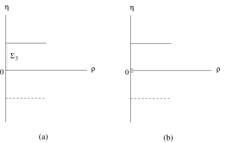
Figure 2: The configurations before and after the transition. In (a) there is a large disk with $N_{2}~{}$units of charge above the infinite disk. In (b) the large disk has $N_{2}-1~{}$units of charge and there is another small disk near origin with $N_{5}$ units of charge. There is a $\Sigma_{3}$ cycle that is along $\rho=0$ and between the disks, formed together with the $S^{2}$. Below the infinite disk, there are image disks.

Since we use an Euclidean brane in a geometric background, such analysis is only an approximation when the transition is very slight or perturbative in nature. The geometries dual to two different vacua are different, so a non-perturbative analysis is generically needed, and it will be discussed in next section. The geometries before and after transition are approximated as the same background in this section. The wrapping of the brane should satisfy DBI-WZ action and global conditions.

We first look at some regimes which obviously can be compared from both sides. We first look at the plane-wave matrix model. We look at in the gauge theory side transition from a vacuum with $N_{2}$ copies of fuzzy spheres with size $N_{5},$ to the vacuum with $N_{2}-1~{}$copies of fuzzy spheres with size $N_{5}$ plus $N_{5}$ copies of size 1 (or a single NS5 brane with $N_{5}~{}$D0 branes). We keep $N_{5}$ moderately large and $N_{2}$ large. In the dual gravity description, each fuzzy sphere is a disk with charge proportional to $N_{2},$ and located at a distance $\eta_{0}=\frac{\pi}{2}N_{5}$ above the $\eta=0$ plane (for more details, see section 2.2 of [10]). In the gravity picture, it corresponds to transition from a large disk with charge $Q=\frac{\pi^{2}}{8}N_{2}~{}$above the $\eta=0$ plane, to a large disk with charge $Q^{\prime}=\frac{\pi^{2}}{8}(N_{2}-1)$ plus a very small disk near the origin (see figure 2). We consider the small disk and its image as a small dipole with dipole moment $2(Q-Q^{\prime})\eta_{0}=\frac{\pi^{3}}{8}N_{5}~{}$near the origin, and that they do not back-react to the geometry. The total dipole moment, which corresponds to $N$ D0 branes, is conserved.

There is a nontrivial 3-cycle at $\rho=0,$ between the large disk and the $\eta=0$ plane. The cycle has topology of an $S^{3},$ with the $S^{2}$ shrinks only at $\eta=0$ and $\eta=\eta_{0}.$ The Euclidean D2 brane wraps the $S^{2}$ and its Euclidean time $\tau$ is embedded along $\eta$ direction extending from $\eta=0$ to $\eta=\eta_{0}.$ We should find $\eta(\tau)$ as a function of $\tau$ from the DBI-WZ action. Such Euclidean branes preserve half of the total 16 supercharges, since they extend along $\eta$ and have an additional projection condition for the Killing spinors. This Euclidean D2-brane has $N_{5}$ Euclidean D0-brane charges, and it mediates the transferring of one unit of D2 charge and $N_{5}$ units of D0 charges, see figure 2. We utilize the general background solution in eqn (2.20-2.24) of [10]. It is parametrized by an electric potential $V$ as a function of $\rho,\eta$.

The DBI part of the action is

$$S_{DBI}/\tau_{2} = -\int d\tau d^{2}\Omega e^{-\Phi}\sqrt{\det G_{\parallel}}\sqrt{\det G_{\perp}+\det(2\pi\alpha^{\prime}F-B)}$$ (3.1)

$$= -\int d\tau 4\pi e^{-\Phi}\sqrt{(-g_{tt})+g_{\eta\eta}(\partial_{\tau}\eta)^{2}}\sqrt{g_{22}^{2}+(\pi N_{5}\alpha^{\prime}-2\eta-\frac{2\overset{\cdot}{V}\overset{\cdot}{V^{\prime}}}{\Delta})^{2}}$$ (3.2)

where $\tau_{2}~{}$is the Euclidean D2 brane tension, $g_{tt},g_{\eta\eta},g_{22}$ are various metric components on the $t$, $\eta,~{}$and$~{}S^{2}~{}$directions in the background [10]. $G_{\parallel},$ $G_{\perp}~{}$are the time component and the spherical components of the pull-back metric, and $\det G_{\perp}=g_{22}^{2}\sin^{2}\theta,$ $2\pi\alpha^{\prime}F-B=(\pi N_{5}\alpha^{\prime}-2\eta-\frac{2\overset{\cdot}{V}\overset{\cdot}{V^{\prime}}}{\Delta})\sin\theta d\theta d\phi$ according to flux quantization. We have chosen the gauge that $2\pi\alpha^{\prime}F-B$ is zero where $\eta$ is at the top disk. Dot and prime are the derivatives w.r.t. $\log\rho$ and $\eta$. The WZ part of the action is

$$S_{WZ}/\tau_{2} = -\int[C_{3}+(2\pi\alpha^{\prime}F-B)\wedge C_{1}]$$ (3.3)

$$= -\int d\tau 4\pi\frac{\overset{.}{4V}}{\overset{..}{V}-\overset{.}{2V}}[-\overset{.}{V}-\overset{.}{V}^{\prime}(\frac{1}{2}\pi N_{5}\alpha^{\prime}-\eta)]$$ (3.4)

Due to the background $H_{3}~{}$flux, the Euclidean D2 brane worldvolume gauge field has a source of $N_{5}~{}$units of magnetic charges, and these are precisely cancelled by the $N_{5}~{}$D0 branes ending on it. This is consistent for wrapping the brane on this cycle. This is similar to the situation of Euclidean D2 branes wrapping on the $SU(2)$ group manifold with $H_{3}~{}$flux discussed in [33].

The expression of the action can be simplified if we expand the electric potential near $\rho\approx 0,$ as

$$V=\sum_{i=0,even}^{\infty}(-1)^{\frac{i}{2}+1}\frac{K_{0}^{(i)}}{\left(i!!\right)^{2}}\rho^{i}=-K_{0}+\frac{K}{4}\rho^{2}-\frac{K^{\prime\prime}}{64}\rho^{4}+...,~{}\ ~{}~{}~{}~{}~{}~{}~{}K\equiv K_{0}^{\prime\prime}$$ (3.5)

where $K$ is only a function of $\eta$. $K$ has some properties such as $K>0,~{}\frac{-8K}{K^{\prime\prime}}>0,$ in order to satisfy the regularity condition for the geometry. The action is then

$$\frac{S_{E}}{4\pi\tau_{2}} = -\int d\tau\left(\frac{-8K}{K^{\prime\prime}}\right)^{\frac{1}{2}}\sqrt{[K+K^{\prime}(\frac{\pi}{2}N_{5}-\eta)]^{2}-\frac{1}{2}KK^{\prime\prime}(\frac{\pi}{2}N_{5}-\eta)^{2}}\sqrt{\frac{-8K}{K^{\prime\prime}}+(\partial_{\tau}\eta)^{2}}$$ (3.6)

$$+\int d\tau\frac{-8K}{K^{\prime\prime}}[K+K^{\prime}(\frac{\pi}{2}N_{5}-\eta)]$$

We have set $\alpha^{\prime}=1$. Since the action does not explicitly depend on $\tau,$ we can have a conserved quantity $H=P\partial_{\tau}\eta-L=\mathrm{const.}=E,$ where $P=\partial_{\partial_{\tau}\eta}L.$ It is obvious that the constant solution $\eta=\frac{\pi}{2}N_{5}~{}$is a special case of a class of solutions to the equations, and from this solution we get $E=0.~{}$Setting $E=0$, we get the equation of motion

$$\partial_{\tau}\eta=-\frac{2K(\frac{\pi}{2}N_{5}-\eta)}{K+K^{\prime}(\frac{\pi}{2}N_{5}-\eta)}$$ (3.7)

The solution for the Euclidean D2 brane is

$$e^{-2\tau}=\frac{K}{(\frac{\pi}{2}N_{5}-\eta)}$$ (3.8)

There could be an overall constant on the RHS, but it can be absorbed by shifting $\tau$.

We plug in the solution back into the action and integrate out to get the final answer of the Euclidean D2-brane action

$$S_{E} = -4\pi\tau_{2}\int_{0}^{\frac{\pi}{2}N_{5}}2K(\frac{\pi}{2}N_{5}-\eta)d\eta$$ (3.9)

$$= -\frac{2}{\pi}[V(\eta_{0})-V(0)-\eta_{0}V^{\prime}(0)]$$ (3.10)

where we used integration by parts several times to arrive at the last expression, and we used $\tau_{2}=\frac{1}{4\pi^{2}},~{}\alpha^{\prime}=1,~{}\eta_{0}=\frac{\pi}{2}N_{5}.$ $V(\eta)$ in the expression is understood as the potential $V(\rho,\eta)$ along the $\rho=0~{}$line. The expression (3.10) has the right property of the invariance under the shift of $V$ by a linear term in $\eta,$ since the gravity solution should be invariant under this shift.

To get more intuition, let’s look at the example of two infinite disks, which is the NS5 brane soultion in [10]. We wrap a Euclidean D2 brane on the throat region of the NS5 brane solution. For that solution [10],

$$V=\frac{1}{\widetilde{g}_{0}}I_{0}(r)\sin\theta,~{}~{}~{}~{}r=\frac{2\rho}{N_{5}},~{}\ ~{}~{}\theta=\frac{2\eta}{N_{5}}$$ (3.11)

where $\widetilde{g}_{0}$ is a constant, so $K=-V^{\prime\prime}|_{\rho=0}={\frac{4}{N_{5}^{2}}}\widetilde{g}_{0}^{-1}\sin\theta.~{}$The action of the Euclidean D2 brane is

$$\frac{S_{E}}{8\pi\widetilde{g}_{0}^{-1}\tau_{2}}=-\int d\tau\sqrt{(\pi-\theta)^{2}(c^{2}+1)+4sc(\pi-\theta)+2s^{2}}\sqrt{8+(\partial_{\tau}\theta)^{2}}+\int d\tau 4[s+c(\pi-\theta)]$$ (3.12)

where $c=\cos\theta,s=\sin\theta$, $\theta\in[0,\pi],~{}$and the equation of motion is

$$\partial_{\tau}\theta=\frac{2(\pi-\theta)s}{s+c(\pi-\theta)}$$ (3.13)

The solution for the Euclidean D2-brane is then

$$e^{-2\tau}=e^{-2\tau_{0}}\frac{\sin(\pi-\theta)}{\pi-\theta}$$ (3.14)

where $\tau_{0}$ is a constant. When $\theta=\pi$, $\tau(\pi)=\tau_{0},~{}$when$~{}\theta=0$, $\tau(0)=+\infty$, so this transition corresponds to transferring a small charge (corresponding to one unit of $N_{2}$) from the top disk to the bottom disk. The Euclidean D2 brane action for this solution is $S_{E}=\frac{2}{\widetilde{g}_{0}}.$

Of course, the solution in the form (3.10) works for general configurations of disks in the plane-wave matrix model, when there are nearby two disks. The Euclidean D2 branes wrapping on that cycle mediate transferring of charges between two disks while keeping the total dipole moment fixed. It also works for the 2+1 d SYM. In that case, the Euclidean D2 brane mediates similar transferring of charges between two nearby disks, while the total dipole moment of the system is kept to zero, because the theory is expanded from the plane-wave matrix model and the disks are already in the center of charge frame.

There are issues of the range of validity that need to be addressed. One is that the calculation of the embedding of the Euclidean D-brane needs that the gravity backgrounds are weakly curved, this requires that the two disks where the cycle is in between are quite large, and their separation is also quite large. This needs the parameters $(g_{ym0}^{2}/m^{3})N_{2},~{}N_{5}$ to be relatively large. On the other hand, $N_{5}~{}$had better not be too large, this is because from the Euclidean D2 brane point of view, there are $N_{5}$ D0 branes ending on its worldvolume, if $N_{5}$ is too large we would consider these $N_{5}$ D0 branes as a single NS5 brane, and the brane configuration should be changed. From the disk point of view the small disk near the origin should be much smaller then the top disk, so $N_{5}\ll N_{2}.$ And these conditions have already guaranteed that the charges on the Euclidean D2 brane are much smaller than the background charges.

A second issue of the range of validity is that the Euclidean brane calculations only describe the transition between very close vacua or very close backgrounds. The geometric backgrounds before and after the transition are approximated as the same geometry. So in principle we need non-perturbative description which could interpolate between very different backgrounds, as long as it is allowed by the condition in section 2. This will be discussed more in section 3.2 in terms of the non-perturbative superpotentials.

The condition for the instanton solution as discussed in section 2 in the gauge theory side is that there are boxes moving from left to right only, in the Young tableaux. The number of boxes are the number of D0 branes transferred. This condition in the gravity side in our case is the transferring of charges from the higher disk to the lower disk. The process in figure 2 corresponds to the illustration in figure 1.

The instantons and Euclidean branes we studied so far describe tunnelings between spherical giant gravitons and point giant gravitons in the 11d plane-wave geometry. This can be related to the limit of those instantons tunneling between spherical giant gravitons and point giant gravitons in $AdS_{4,7}\times S^{7,4}$ studied by [35], [36], (see also [37]). The difference is that the giant gravitons ([34],[35],[36]) in their analysis of the tunneling are probe branes in the $AdS_{4,7}\times S^{7,4}$ geometries and in our case we have replaced the giant gravitons with the back-reacted geometries taking into account the back-reaction of them on the plane-wave geometry. It is analyzed both in [35] and [21] that these instantons have 8 supersymmetries, and are 1/4 BPS objects from the point of view of the asymptotic geometries. In our case, the kappa symmetry condition on the Euclidean D2 brane will impose an additional projection condition, with respect to the one for the background. Again, there will be at least 8 fermionic zero modes corresponding to the broken supersymmetries and the fermionic zero modes suppress the tunneling amplitude and forbid the mixing of the vacua.

One can also consider an Euclidean NS5 brane wrapping a six-cycle enclosing the disk, which is the $\Sigma_{6}$ cycle in [10]. This Euclidean NS5 brane has $N_{2}~{}$units of Euclidean D0 charges. It interpolates between a vacuum of $N_{5}$ NS5 branes with size $N_{2}~{}$and the vacuum with $N_{5}-1$ NS5 branes with size $N_{2},~{}$plus $N_{2}~{}$D0 branes. On the gravity side, the transition corresponds to lowering the disk by one unit of the height. This instanton solution is allowed from gauge theory side but its action is zero in the weak coupling limit. From the gravity side and strong coupling point of view, the action should be non-zero. The existence of this Euclidean NS5 brane is a quantum effect from gauge theory point of view. Since the upper surface and lower surface of the disk are treated differently, it is more convenient to use the coordinates of the $x_{1}=x_{11},~{}x_{2}=V^{\prime},~{}y=\overset{.}{V}$ appeared in the Toda equation [7],[10]. From 11d point of view, it’s a Euclidean M5 brane wrapping $S^{5},$ with its worldvolume $\tau~{}$extending along $x_{2}~{}$of the M5 strip at $y=0$ and traveling along the $x_{1}$ circle, with $N_{2}~{}$units of momenta $P_{x_{1}}$ conjugate to $x_{1}$. From the point of view of the IIA Euclidean NS5 brane, there is a worldvolume scalar corresponding to $x_{1},$ and the action [38] can be written as

$$S_{E}/\tau_{5} = -\int d\tau d^{5}\Omega e^{-2\Phi}\sqrt{(-g_{tt})+g_{x_{2}x_{2}}(\partial_{\tau}x_{2})^{2}+e^{2\Phi}\mathcal{F}_{\tau}^{2}}\sqrt{\det g_{55}}+\int[B_{6}+C_{5}\wedge\mathcal{F}]$$

$$\mathcal{F} = (\partial_{\tau}x_{1}-C_{t})d\tau$$ (3.15)

where $\tau_{5}=\frac{1}{(2\pi)^{5}},\alpha^{\prime}=1,~{}g_{tt},~{}g_{x_{2}x_{2}},~{}g_{55}$ are the components of the metric along the $t,$ $x_{2},~{}S^{5}~{}$directions, $B_{6},C_{5}$ are the pull-backs of the potentials dual to $B_{2},C_{3},~{}$and$~{}\mathcal{F}$ is the worldvolume one-form flux. We look at solutions that $P_{x_{1}}=\frac{\partial L_{\tau}}{\partial(\partial_{\tau}x_{1})}=\frac{N_{2}}{R_{11}},$ that is quantized into integers $N_{2}~{}$corresponding to D0 charges, and then the equation of motion will yield $x_{2}(\tau)$ as a function of $\tau,$ which characterizes the embedding of the brane. If we expand the solution near an isolated disk, we can approximate it by the solution of a single disk, which was the solution (2.49)-(2.54) of [10] corresponding to the 2+1 d SYM. Using this solution, we then estimate the action to be $S_{E}\sim g_{ym2}^{-4}(g_{ym2}^{2}N_{2})^{4/3}\sim g_{ym0}^{-4}\eta_{0}^{2}\rho_{0}^{4},$ where $\eta_{0}~{}$and $\rho_{0}~{}$are the height and size of the disk, and $g_{ym0}=g_{0}$ is the coupling constant in the plane-wave matrix model. This is a quantum effect and strong coupling result which is not seen in the weak-coupling gauge theory.

3.2 Electric charge system and superpotential

Now we analyze what the quantity $W$ is in the electrostatic picture. In the gauge theory, the instanton action is proportional to the difference of the superpotentials of the two vacua as defined by $S_{inst}=-\frac{1}{g_{0}^{2}}\Delta W~{}$in (2.7).  In the case of the two vacua that is very similar to each other, we used the approximation of an Euclidean brane action to match the instanton action. Of course, the Euclidean brane action will be the strong-coupling result. For the configuration of two vacua studied in section 3.1, involving the exchange of a unit of charge (corresponding to a unit of $N_{2}$) between two disks, we arrived at the expression

$$S_{E}=-\frac{2}{\pi}[V(\eta_{0})-V(0)-\eta_{0}V^{\prime}(0)]$$ (3.16)

This quantity is proportional to the change of the total energy $U$ in the electrostatic system (including image charges). Note that the relation between D2 brane number and electric charge is $Q=\frac{\pi^{2}}{8}N_{2}~{}$[10], so the charges are in units of $\frac{\pi^{2}}{8}$, the charge transfer in this process is $\Delta Q=\frac{\pi^{2}}{8}.$ The energy that the unit charge and its image charge released is

$$-\Delta U_{\mathrm{ch}\arg\mathrm{e}}=2\Delta Q[V(\eta_{0})-V(0)]$$ (3.17)

On the other hand, the total dipole of the charge system is conserved, the dipole had been lost by the amount $2\Delta Q\eta_{0}$ by transferring the unit charge from the top disk. After the transferring process, we have the small disk (and also its image disk) near the origin, as in figure 2(b). We make an approximation when a pair of small disks near the origin is approximated as a point. We thereby have a small dipole with dipole moment $2\Delta Q\eta_{0}$ at the origin. The electric field at the origin is $-V^{\prime}(0),$ which is pointing upward, so the coupling between the dipole and the electric field there gives an negative energy, this is the energy the dipole released:

$$-\Delta U_{\mathrm{dipole}}=(2\Delta Q\eta_{0})[-V^{\prime}(0)]$$ (3.18)

So the total energy difference of the system between final and initial configuration is

$$\Delta U_{\mathrm{total}}=-2\Delta Q[V(\eta_{0})-V(0)-\eta_{0}V^{\prime}(0)]$$ (3.19)

which is just proportional to the Euclidean D2 brane action, in appropriate unit. Of course this definition of the change of the total energy is invariant under the shift of the potential $V~{}~{}$by a linear term$~{}b\eta.$ The energy difference will not be changed due to this shift of $V$. This is because the charge $\Delta Q,$ will release an additional energy $2\Delta Qb\eta_{0},$ on the other hand, due to that there is an additional electric field downward with magnitude $b,$ the dipole’s energy is increased by $2\Delta Q\eta_{0}b,$ which exactly cancels the additional energy released from the charge. So this expression is consistent with the definition of the change of the total energy.

We therefore can identify (in the strong coupling regime) $S_{inst}=S_{E}=\frac{8}{\pi^{3}}\Delta U,$ and thereby the superpotential for each vacuum can be defined in terms of the energy of the electric configuration corresponding to that vacuum

$$U=-\frac{\pi^{3}}{8g_{0}^{2}}W$$ (3.20)

up to an overall constant shift which is not important when comparing differences. The minus sign is due to our conventions. So the superpotential of the system is proportional to the total energy of charges (including image charges)

$$W=-\frac{16g_{0}^{2}}{\pi^{3}}\sum_{i}Q_{i}V_{i}$$ (3.21)

and $W_{0}$ which corresponds to the single NS5 brane vacuum is set to zero for convenience. $i$ represents different groups of charges at $\eta=\eta_{i}~{}$with potential $V_{i}.$ Now we see that the factor of the instanton amplitude is given by the energy difference between the two configurations of the electric charge system or the eigenvalue system. The factor in the instanton amplitude is largely suppressed if the energy difference is large. Note that there are still other parameters like the $\alpha^{\prime}$ and $\hbar,$ which have been set to 1 for convenience. These charges are associated with eigenvalues from the $SO(6)$ scalars and will be discussed in section 4.

It might be useful to notice that the expressions (3.21) can be reduced to integrals of forms in $\rho,\eta$ space. We define one forms locally $dV=\partial_{\eta}Vd\eta+\partial_{\rho}Vd\rho,~{}dq=2\pi\rho\ast_{2}dV=2\pi(-\partial_{\eta}V\rho d\rho+\partial_{\rho}V\rho d\eta),~{}$where $\ast_{2}$ is the flat space epsilon symbol in $\rho,\eta$ space. The Laplace equation for $V$ is just $d(dq)=0.$

We choose one-cycle $\Pi_{i}~{}$enclosing each disk, and one-cycle$~{}\Gamma_{i}$ between each disk and a reference disk (whose potential is set as zero). We see that

$$Q_{i}=\int_{\Pi_{i}}dq,~{}~{}~{}~{}\ ~{}~{}V_{i}=\int_{\Gamma_{i}}dV$$ (3.22)

Since $\Pi_{i}$ cycle and the $S^{5}$ forms a 6-cycle, and $\Gamma_{i}$ cycle and $S^{2}$ forms a 3-cycle in 9 spatial dimensions, the $\Pi_{i}$ and $\Gamma_{i}$ cycles do not intersect,$~{}\Pi_{i}\cap\Gamma_{i}=0.$ We can thereby form a two-cycle by the cup product of the two cycles, so (3.21) can be written as

$$W=-\frac{16g_{0}^{2}}{\pi^{3}}\int_{\Pi_{i}\cup\Gamma_{i}}dq\wedge dV=-\frac{16g_{0}^{2}}{\pi^{3}}\int_{\Pi_{i}\cup\Gamma_{i}}|\nabla V|^{2}2\pi\rho d\rho\wedge d\eta$$ (3.23)

where $\nabla V$ is the gradient of $V$ in $\rho,\eta$ space. So we have defined the superpotential of a boundary gauge theory by purely forms appeared in the bulk of gravity duals. This view is very similar in spirit to the definition of the non-perturbative superpotential in 3+1 d $\mathcal{N}=1$ gauge theories via a flux background after geometric transition, e.g. [42].

Let’s compare the superpotential in the weak coupling case. The charges in the electric system originate from the eigenvalues of the matrices in the $SO(6)$ sector in the gauge theories. We will discuss this more in section 4. Classically, these eigenvalues do not interact with each other. They distribute under the external electric potential, which are quadratic ($\sim\rho^{2}$) in the gravity dual of either theories [10]. So they are sitting on top of each other at fixed position $\eta_{i}$ at $\rho=0$. Quantum mechanically, the eigenvalues repel each other and they are not coincident. They thus form extended disks. The classical and quantum pictures, correspond to weak coupling and strong coupling effects for the superpotential. In the weak coupling analysis, the superpotential does not involve any dependence on the $SO(6)$ scalars, so this must get corrections when coupling increases and becomes large.

For the plane-wave matrix model, the background potential is $V_{b}=\frac{8}{g_{s}}(\rho^{2}\eta-\frac{2}{3}\eta^{3}),$ where $g_{s}=4\pi^{2}g_{ym0}^{2}$ (e.g. [43]) and $g_{s}$ is the string coupling that appears at the asymptotic D0 brane near horizon geometry [44]. Since in the gravity side, $m$ is the unit of energy for $\frac{|g_{tt}|}{g_{55}}$ [10], which is 1 in our case, so we have $m=1.~{}$In the weak-coupling regime of the gauge theory, since the charges sit at $\rho=0~{}$and$~{}\eta=\eta_{i},$ they feel potential $V_{i}=-\frac{4}{3\pi^{2}g_{0}^{2}}\eta_{i}^{3},$ so the superpotential from (3.21) is:

$$W=\frac{64}{3\pi^{5}}\sum_{i}Q_{i}\eta_{i}^{3}=\sum_{i}\frac{1}{3}N_{2}^{(i)}N_{5}^{(i)3}$$ (3.24)

where we used$~{}N_{2}^{(i)}=\frac{8Q_{i}}{\pi^{2}},~{}N_{5}^{(i)}=\frac{2\eta_{i}}{\pi}~{}$[10] from flux quantization conditions. This is the same as the field theory calculation in weak-coupling regime, cf. (2.9).   The factor of the instanton amplitude is largely suppressed if $g_{s}$ is small and the change of the energy of the system is large.

Figure 3: Comparison of strong coupling and weak coupling superpotentials. In (a) the charges or eigenvalues are extended into disks due to eigenvalue interactions in strong coupling regime. In (b) they are on top of each other at $\rho=0~{}$line and not extended in the $SO(6)$ directions in the weak coupling limit. The superpotential is given by the energy of the electric charge system.

The vacua of the 2+1 d SYM are inherited from that of plane-wave matrix model. In the disk configuration of the plane-wave matrix model, if we look at the geometry locally near a group of disks that is isolated from all other disks, including their images, then the geometry locally approaches to the solution dual to 2+1 d SYM theory. The vacuum of the 2+1 d SYM thereby is also characterized by the total energy of the electrostatic system. A special case is that when we start from plane-wave matrix model and look at the configuration where all the disks are very high above $\eta=0$ plane and they are relatively near each other. Their average position is $\eta_{0}=\frac{\pi}{2}\overline{N}_{5}$. We define new coordinate relative to the average position $\widetilde{\eta}=\eta-\eta_{0}=\frac{\pi}{2}n_{5},~{}(\widetilde{\eta}\ll\ \eta_{0})~{}$and $n_{5}=N_{5}-\overline{N}_{5},~{}(n_{5}\ll\overline{N}_{5})$. The total number of the D2 brane charges is $N_{2}=\sum_{i=disks}N_{2}^{(i)}.~{}$So in the new coordinate frame,  this is the configuration dual to the $U(N_{2})$ 2+1 d SYM. $n_{5\text{ }}$is proportional to the location of each disk in the new frame. The case with all $n_{5}=0$ corresponds to a single disk at $\widetilde{\eta}=0,$ and is the simplest vacuum with unbroken $U(N_{2}).$The number $\overline{N}_{5}$ is used in the matrix regularization for the $S^{2}.$ The electric potential near this group of disks is

$$V=\frac{2}{\pi^{2}g_{0}^{2}}(\rho^{2}\eta-\frac{2}{3}\eta^{3})=\frac{2\eta_{0}}{\pi^{2}g_{0}^{2}}(\rho^{2}-2\widetilde{\eta}^{2})-\frac{4}{3\pi^{2}g_{0}^{2}}\eta_{0}^{3}+...$$ (3.25)

They basically feel the same external potential $\frac{2\eta_{0}}{\pi^{2}g_{0}^{2}}(\rho^{2}-2\widetilde{\eta}^{2})~{}$as in the gravity dual of the 2+1 d SYM theory discussed in [10], with a large constant shift due to our expansion. The dot terms are the linear term in $\widetilde{\eta}$ and higher order terms in $\widetilde{\eta},$ which are not important.

In the weak coupling regime, the charges are not extended in the $\rho$ direction. The total energy of the system (excluding the large constant term) gives the superpotential from the relation (3.21)

$$W=-\frac{16g_{0}^{2}}{\pi^{3}}\sum_{i}Q_{i}~{}\frac{2\eta_{0}}{\pi^{2}g_{0}^{2}}(-2\widetilde{\eta}_{i}^{2})=N_{2}\overline{N}_{5}\sum_{i}n_{5}^{(i)2}$$ (3.26)

The large constant term from the $\eta_{0}^{3}$ term in the electric potential, corresponds to $W_{J_{i}}=\sum_{i}\frac{4}{3}~{}\mathrm{tr}_{N\times N}J_{i}^{2}$ term for the fuzzy sphere we are expanding around in the plane-wave matrix model, cf. (2.15).

We thereby find that the weak-coupling superpotential analyzed in section 2, which does not involve $SO(6)~{}$scalars, is the situation in the gravity side when the eigenvalues are not extended in the $\rho$ direction, or the $SO(6)$ directions. This is when the eigenvalues do not have interactions between each other. To bring in the interactions, we need quantum effect, and this is shown in the strong coupling regime in the disk picture. These are illustrated in figure 3.

Now we briefly discuss some technical aspects of solving the value of the superpotential in the strong-coupling regime, for the disk configurations. We first discuss the situation with a single disk above $\eta=0$ plane (3.10), and then the situation with some arbitrary numbers of disks (3.21).

We first discuss the situation of a pair of positively and negatively charged disks under the background potential $V_{b}=\frac{8}{g_{s}}(\rho^{2}\eta-\frac{2}{3}\eta^{3}).$ The size of the disks is $\rho_{0}$ and their separation is $2\eta_{0}.$ Apart from the background, the charges have mutual repulsions from other charges on the disk and attractions from the image disk. Suppose the charge density and the potential on the disk is $\sigma(\rho)$ and $V_{0}.$ We can scale out everything and the problem then is only determined by the ratio $\kappa=\frac{\eta_{0}}{\rho_{0}}.$ We make the rescaling$~{}y=\eta/\rho_{0},~{}x=\rho/\rho_{0},~{}\ \sigma(\rho)=\frac{8}{g_{s}}\rho_{0}^{2}g(x),~{}V=\frac{8}{g_{s}}\rho_{0}^{3}v.$

The integral equation in these variables is (which involves dimensionless functions only)

$$\{(x^{2}\kappa-\frac{2}{3}\kappa^{3})+\int_{0}^{2\pi}\int_{0}^{1}[\frac{g(x^{\prime})x^{\prime}dx^{\prime}d\phi}{\sqrt{x^{2}-2xx^{\prime}\cos\phi+x^{\prime 2}}}-\frac{g(x^{\prime})x^{\prime}dx^{\prime}d\phi}{\sqrt{x^{2}-2xx^{\prime}\cos\phi+x^{\prime 2}+4\kappa^{2}}}]\}_{\forall x\in[0,1]}=\mathrm{const.}$$ (3.27)

with the supplementary condition that $g(1)=0$ due to vanishing of the charge at the edge of the disk. When $g(x)$ is solved, it is also a function of $\kappa$.

The integral equation is very difficult to solve due to its complicated kernel. Provided we know the function $g(x),$ since we already know the total charge of the disk, what we need to compute is the potential $V$ on the disk. Since the disk is an equipotential surface, we can know it from the potential at $\rho=0,$ this consists of a contribution from the background and a contribution from the charges. The value of the superpotential (3.21) is

$$W/(\frac{1}{3}N_{2}N_{5}^{3})=1-\frac{2}{3}\kappa^{-3}2\pi\int_{0}^{1}dx~{}g(x)\left[1-\frac{x}{(x^{2}+4\kappa^{2})^{1/2}}\right]$$ (3.28)

It contains two terms. The first term “1” on the RHS gives a contribution to the superpotential that is the same as the weak coupling gauge theory result $W=\frac{1}{3}N_{2}N_{5}^{3}$, it’s the result if the charges were all sitting at $\rho=0.~{}$The second contribution is from the integral term, resulted from the effect of mutual interactions among charges. We do not assume that $\kappa$ has to be small, so in principle, if we were looking for perturbative corrections to the weak coupling answer, the integral term gives the corrections relative to the first piece, in the large $\kappa~{}$regime. The $\kappa$ depends on $N_{2}$ in a very non-linear way. In the small $\kappa$ limit, it is estimated in [10] that $\rho_{0}^{4}=\frac{1}{2}\pi^{4}g_{ym0}^{2}N_{2},~{}\eta_{0}=\frac{\pi}{2}N_{5},$ so $\kappa=\frac{\pi}{2}N_{5}(\frac{1}{2}\pi^{4}g_{ym0}^{2}N_{2})^{-1/4}$.

The problem of solving the integral equation has been simplified by Abel transforming the kernel in (3.27) as done in [18]. The new integral equation is

$$f(x)-\int_{-1}^{1}{\frac{1}{\pi}}{\frac{2\kappa}{4\kappa^{2}+(x-t)^{2}}}f(t)dt=1-2\alpha x^{2}$$ (3.29)

where $f(t)$ is the Abel transform of $g(x)$, $~{}f(t)={\frac{2\pi}{\beta}}\int_{t}^{1}{\frac{rg(r)dr}{(r^{2}-t^{2})^{\frac{1}{2}}},}$ $\beta=v_{0}+\frac{2}{3}\kappa^{3},$ with the additional condition $f(1)=0,~{}f^{\prime}(1)$ is bounded [18], and $\alpha$ is a constant determined by these boundary conditions. The new kernel is the one appears in the Love’s integral equation [48],[49],[50]. The solution in this form seems very promising. The kernel can even be simplified a little bit more in the small $\kappa$ limit [49].

Now let’s discuss the calculation of the superpotential for the electrostatic configuration with an arbitrary number of disks. Once we specify the charges $Q_{i}~{}$of the disks and their heights $\eta_{i}$, what we need to know is the electric potential of each disk $V_{i},$ in order to compute the superpotential (3.21). We can thereby use the conformal transform techniques in [10].

In [10], the complex variables were introduced: $w=2\partial_{z}V=\partial_{\rho}V-i\partial_{\eta}V~{}$and$~{}z=\rho-\rho_{0}+i\eta.$ In the large disk limit, the general solution for the plane-wave matrix model is

$$\partial_{w}z=\prod\limits_{j=1}^{n}\frac{(w-ia_{j})}{(w-ic_{j})}(-ia_{n+1})$$ (3.30)

where there are $n$ finite disks located at $ia_{j},$ and $n$ fivebrane throats located at $ic_{j},~{}$and finally the infinite disk at $ia_{n+1}.$ We can integrate it to get the potential of each disk

$$V_{i}=\mathop{\mathrm{R}e}\int wdz=-\mathop{\mathrm{R}e}\int_{ia_{i}}^{ia_{n+1}}\prod\limits_{j=1}^{n}\frac{(w-ia_{j})}{(w-ic_{j})}(-ia_{n+1})wdw$$ (3.31)

and then plug this in (3.21). The rest is to figure out the relation between $a_{i},c_{i}$ and $N_{2}^{(i)},N_{5}^{(i)}~{}$[10].

4 Emergence of gravity picture and eigenvalue system

In the previous sections, we find that the instanton action is associated with the superpotential of each vacuum, which is in turn related to the emergence of the geometries. The geometries are emergent from matrices in these theories. There are different types of emergence in our cases. The emergence of odd dimensional spheres and the even dimensional spheres seem to be different in some cases. In this section, we will discuss qualitatively the emergence of the extra coordinates and the electrostatic picture.

For the plane-wave matrix model, we have to explain the emergence of 9 directions, $S^{2},~{}S^{5}$, $\eta~{}$and $\rho$. We first discuss the emergence of $S^{2}$ in the plane-wave matrix model. This is by the $SU(2)$ commutation relations of $J_{i}~{}$(e.g. [32]). Other higher even dimensional spheres may similarly emerge in theories constructed using higher even dimensional fuzzy spheres for example [51],[52].

These fuzzy two-spheres have radial motions, which are characterized by the scalar $\Phi,$ most conveniently seen in the 2+1 d SYM. Comparing sections 2 and 3, we find that the eigenvalues of $\Phi$ are proportional to $n_{5}^{(1)},n_{5}^{(2)},...,n_{5}^{(N_{2})},$ which map to the heights of each disk in $\eta$ direction:$~{}\eta_{1},\eta_{2},...,\eta_{N_{2}}.$ So the $\eta$ direction is emerged from the eigenvalues of $\Phi$.

Next we come to the emergence of the odd dimensional sphere $S^{5}~{}$and the direction $\rho.$ From intuition, due to the reduction from $\mathcal{N}=4$ SYM, the $SO(6)$ sector in these theories are quite similar to $\mathcal{N}=4$ SYM. So the emergence of $S^{5}$ should be similar to that of $\mathcal{N}=4$ SYM [4].

In order to address this problem, we embed these vacuum geometries into the larger sector of 1/8 BPS geometries. These 1/8 BPS geometries are dual to 1/8 BPS states in these gauge theories. We can look at 1/8 BPS states satisfying $E-(J_{A}+J_{B}+J_{C})=0,$ where $E$ is the energy and $J_{A},J_{B},J_{C}$ are the three $U(1)$ $R$-charges associated with the excitations by three complex scalars from the $SO(6)$ scalars. These 1/8 BPS states are in turn embedded in an even larger Hilbert space. Finally our BPS vacuum geometries are the ground states in the 1/8 BPS sector.

Though quite similar, a difference of the theories we analyzed, relative to $\mathcal{N}=4$ SYM on $S^{3}\times R,$ is that we have many ground state geometries characterized by a broken gauge symmetry $U(N)\rightarrow\prod\limits_{i}U(N^{(i)}).$ The most convenient theory is the 2+1 d SYM where a particular vacuum is specified by the eigenvalues of the scalar $\Phi.$ If there are $N^{(i)}$ coincident eigenvalues, then there is a $U(N^{(i)})$ symmetry. These eigenvalues form an extended disk in the electric charge picture, but this could have alternative descriptions if we embed the geometries into larger sectors. If the disks are far away from each other, the repulsion of charges on each disk is quite similar to the case of a single disk. In this limit, we study only the case of a single disk, that is, we look at the block of the $SO(6)$ scalars corresponding to $N^{(i)}$ and only excite $U(N^{(i)})$ invariant 1/8 BPS states. Then finally we can excite all the blocks and build $\prod\limits_{i}U(N^{(i)})$ invariant 1/8 BPS states.

For our purposes, we can consider first a single disk vacuum in the 2+1 d SYM with unbroken $U(N)~{}$symmetry, and then other cases will be quite similar. These 1/8 BPS states can be described by the harmonic oscillators of the $SO(6)$ scalars and only s-wave modes of the $S^{2}$ are relevant for this class of BPS excitations. We use the methods similar to those of [4],[5],[6]. The action that is relevant for these excitations of $SO(6)$ scalars is the matrix quantum mechanics

$$S=\frac{\pi}{g_{ym2}^{2}/m}\int dt~{}\mathrm{tr}\left(\frac{1}{2}\overset{\cdot}{X_{a}}\overset{\cdot}{X_{a}}-\frac{1}{2}X_{a}X_{a}+\frac{1}{4}[X_{a},X_{b}]^{2}\right)$$ (4.1)

where $a,b=4,5,...,9$ and we have set $\mu=2$ in the lagrangian. We set $A_{0}=0$ and have a Gauss law constraint on $U(N)~{}$gauge singlet physical states, $\frac{\delta L}{\delta A_{0}}\left|\Psi\right\rangle=0.~{}$Furthermore, the commutator terms will not be included in this class of BPS excitations because they contribute positively to the energy but not the $R$-charges. Then we define the conjugate momenta $P_{a}~{}$for each $X_{a}.~{}$The energy and $R$-charges are

$$E = ~{}\frac{1}{2}\mathrm{tr~{}}(P_{a}P_{a}+X_{a}X_{a}),~{}~{}~{}J_{A}=\mathrm{tr~{}}(P_{4}X_{5}-P_{5}X_{4}),~{}$$ (4.2)

$$J_{B} = \mathrm{tr~{}}(P_{6}X_{7}-P_{7}X_{6}),~{}~{}~{}J_{C}=\mathrm{tr~{}}(P_{8}X_{9}-P_{9}X_{8})$$ (4.3)

We can form the usual three complex scalars $Z_{L},$ and their conjugate momenta $\Pi_{L}=-i\frac{\partial}{\partial Z_{L}^{\dagger}},~{}(L=A,B,C).$ They satisfy the standard commutation relations$~{}[Z_{L}^{mn},\Pi_{L}^{\dagger m^{\prime}n^{\prime}}]=i\hbar\delta_{nm^{\prime}}\delta_{n^{\prime}m},~{}[Z_{L},\Pi_{L}]=0,$ so we can define creation/annihilation operators

$$a_{L}^{\dagger}=\frac{1}{\sqrt{2}}(Z_{L}^{\dagger}-i\Pi_{L}^{\dagger}),~{}~{}\ \ b_{L}^{\dagger}=\frac{1}{\sqrt{2}}(Z_{L}^{\dagger}+i\Pi_{L}^{\dagger})~{}$$ (4.4)

and their conjugates. The energy and $R$-charge operators are then written as

$$E=\mathrm{tr}\sum_{L}(a_{L}^{\dagger}a_{L}+b_{L}^{\dagger}b_{L}),~{}~{}~{}J_{L}=\mathrm{tr~{}}(a_{L}^{\dagger}a_{L}-b_{L}^{\dagger}b_{L})$$ (4.5)

So it’s clear in order to get 1/8 BPS states, we should keep only the three $a_{L}^{\dagger}$ oscillators but not the three $b_{L}^{\dagger}$ oscillators. We have then in this 1/8 BPS subspace of the Hilbert space a three dimensional harmonic oscillator Hilbert space. Its phase space is six dimensional. The singlet condition tells us that we should look at states of products of traces

$$\left|\Psi\right\rangle=\prod\limits_{j=1}^{k}\mathrm{tr~{}}(a_{A}^{\dagger})^{l_{j}}(a_{B}^{\dagger})^{m_{j}}(a_{C}^{\dagger})^{n_{j}}\left|0\right\rangle~{}$$ (4.6)

with $l_{j},m_{j},n_{j}\leqslant N$. Because the commutator terms vanish, by unitary transformations we may simultaneously put $Z_{A},Z_{B},Z_{C}$ into the form of triangular matrices, each of which is a sum of a diagonal matrix and an off-diagonal triangular matrix. We integrate out the unitary matrices and also the off-diagonal triangular matrices. Let the diagonal matrix elements be $z_{Ai},z_{Bi},z_{Ci}.~{}$The wave function corresponding to (4.6) is of the form

$$\Psi\sim\Delta(z_{Ai},z_{Bi},z_{Ci})\prod\limits_{j=1}^{k}\mathrm{~{}}(\sum_{i}z_{Ai}{}^{l_{j}})(\sum_{i}z_{Bi}{}^{m_{j}})(\sum_{i}z_{Ci}{}^{n_{j}})e^{-\frac{1}{2}\sum_{i}z_{Ai}{}\overline{z}_{Ai}{}+z_{Bi}{}{}\overline{z}_{Bi}{}+z_{Ci}\overline{z}_{Ci}{}}~{}$$ (4.7)

up to some normalization factors, including the factor from integrating out off-diagonal matrices. $\Delta(z_{Ai},z_{Bi},z_{Ci})$ is a Van-de-monde determinant from integrating out unitary matrices. See similar wave functions in [4], and its 1/2 BPS case [5],[6],[58],[59],[60]. There is an interesting property. The wave function, besides the universal Gaussian factor, is a holomorphic function in $z_{Ai},z_{Bi},z_{Ci},$ due to the 1/8 BPS condition. This holomorphicity provides some simplifications in the wave functions. Wave functions that depends also on ${}\overline{z}_{Ai}{},{}{}\overline{z}_{Bi}{},{}\overline{z}_{\mathop{\mathrm{C}i}}$ are non-BPS. The complex structure is related to the symplectic structure in the phase space $C^{3}.$ Each $z_{Li}~{}$coordinates in the phase space are paired by a physical real coordinate and its conjugate momentum, $z_{Li}=x_{Li}+ip_{Li}$ [4].

In the large $N$ limit, the wave function has a thermodynamic interpretation, the wave function squared describes the probability of a particular eigenvalue distribution in phase space [4]. The saddle point approximation of the wave function gives a droplet configuration in the phase space. The polynomial part of the wave function provides repulsion forces between eigenvalues. The Gaussian factor gives a spherically symmetric quadratic potential. The ground state should be a spherically symmetric droplet with $SO(6)$ symmetry in $C^{3}$, which is bounded by an $S^{5}.$ Because of the spherical symmetry of the ground state droplet, the $S^{5}$ emerges in the gravity description. We see that the eigenvalues are extended in the radial direction of $R^{6},~{}$the $\rho$ coordinate in the gravity description is really mapped from the radial direction of the phase space $R^{6}.$ In the electric charge picture, charges are extended along $\rho,$ if we tensor the $\rho$ with the $S^{5}$, the charges are really distributing in a six dimensional space. The electric disks emerge from the eigenvalues of the $SO(6)$ matrices. This would be more clear if we had all the regular 1/8 BPS geometries of these theories. The $S^{5}$ then will be a particular enhanced symmetry for only the ground state geometries.

If we start from 1/4 BPS sector or 1/2 BPS sector, we will have similar but reduced droplet descriptions. They are described by two or one dimensional harmonic oscillators similar to the discussion above. They will have a $C^{2}$ or $C^{1}$ phase space. The ground state droplet will have $SO(3)$ symmetry in $R^{4}$ bounded by an $S^{3}~{}$or $U(1)$ symmetry in $R^{2}~{}$bounded by an $S^{1}.$ In the electrostatic picture, there is an $S^{1}$ isometry from the $S^{5},$ that could combine with $\rho$ into a real two dimensional disk. If we had all the 1/2 BPS geometries for these theories, they should have a $S^{3}~{}$isometry out of $S^{5}.$ The ground states have an enhanced symmetry of $S^{1}~{}$which combines $\rho~{}$to form a disk. Small ripples on the edge of the disk then describe BPS particles traveling along the $S^{1}~{}$equator of the $S^{5}.$ We have a further evidence from the 3+1 d $U(N)$ $\mathcal{N}=4$ SYM on $R\times S^{3}/Z_{k}$ with $k/N$ small. In the electrostatic picture, the vacuum are periodic disks. If we look at the vacuum with one disk in a single period, because $k/N$ is small, they look like charges in a cylinder, and the Laplace equation will be two dimensional in the space of $\rho$ and an $S^{1}.$ On the disk, the charges feel logarithmic repulsions plus an spherical symmetric quadratic potential. The integral equation for the equilibrium configuration is exactly the same as the one in eqn (2.16) of [4] for the 1/2 BPS ground state droplet of $\mathcal{N}=4$ SYM on $R\times S^{3}$. We see that their descriptions are consistent and should be exactly the same for $k=1$.

These ideas should be compared with the gravity results. A class of 1/4 BPS and 1/8 BPS geometries in $\mathcal{N}=4$ SYM, relevant to the matrix model discussed above, have been studied by [61],[62] and by [63]. They have $U(1)\times SO(4)\times SO(2)_{R}$ [61],[62] and $U(1)\times SO(4)~{}$symmetries [63] (after analytical continuation of $AdS_{3}$) respectively. A Kahler structure were observed in both cases. In the 1/4 BPS case, it was reduced to a five dimensional Monge-Ampère type equation which is highly non-linear. The boundary condition is roughly to divide regions where the $S^{3}$ or $S^{1}$ shrinks smoothly. Thereby there could be a droplet configuration in a four dimensional space. However, the regularity condition and the topology of these solutions are very complicated. To understand the differential equation in terms of the emergent forces between eigenvalues is a very challenging problem. Our case of the emergence of the electric charge picture of eigenvalues from gauge theories may bear some similarities to these more complicated cases.

The emergence of the odd dimensional sphere from phase space discussed above can be generalized to other cases, for example $S^{7}$. We consider the emergence of $AdS_{4}\times S^{7}$ from M2 brane theory on $R\times S^{2}.$ Apart from the time and $S^{2}$ that are already present, we need to explain the radial coordinate $r$ in $AdS_{4}$ and the $S^{7}.~{}$We can look at the 1/16 BPS states of the M2 brane theory, by looking at a BPS bound in which energy is bounded by the sum of 4 $U(1)$ $R$-charges out of $SO(8)_{R}$. They correspond to excitations of four oscillators associated with the 4 complex scalars for the 1/16 BPS chiral primary states. The 1/16 BPS sector has an eight dimensional phase space. The ground state droplet should have an enhanced symmetry of $S^{7}$ in the phase space. Similar picture for the 1/2 BPS sector of M2 brane theory has been studied in [7], the emergence of the $S^{1}~{}($part of $S^{7})~{}$for the ground state in a two-plane has been observed.

Other ways of emergence of odd dimensional spheres, similar to the even dimensional ones, have been studied by for example [64],[52],[65]. Their emergence is similar to the $S^{2}$ in our cases.

5 Conclusion and discussions

In this paper we studied the vacua of gauge theories and the dual gravity descriptions of each vacuum. These theories are $U(N)$ plane-wave matrix model and 2+1 dimensional SYM on $R\times S^{2}$. They have a large number of supersymmetric vacua. Each vacuum can be consistently lifted to the $\mathcal{N}=4$ SYM on $R\times S^{3},$ where they become pure gauge transformations of the vacuum of the $\mathcal{N}=4$ SYM [10]. There exist instanton solutions interpolating some of these vacua. Explicit instanton solutions are known. The conditions for allowed instanton solutions are determined by the initial and final vacua and the gauge group. In the representation of Young tableaux, the condition becomes moving a number of boxes from left to right only. The instanton actions are the difference of superpotentials of initial and final vacua. We compute the superpotential of each vacuum on the weak coupling gauge theory side, and they are traces of some operators and their final answers depend on the coupling and the numbers like the $N_{2}^{(i)},N_{5}^{(i)}$.

We then study the description of these instantons in gravity duals. In the case where initial and final vacua are very close to each other, the instanton can be approximated as an Euclidean brane wrapping certain cycle in the gravity dual background. Each gravity background dual to the vacuum is given by the configuration of an electric charge system where the charges distribute on disks under an external quadratic potential. The action of such Euclidean D2-brane wrapping a three-cycle shows that it is the energy difference between initial and final configurations of the electrostatic system. We thereby are able to know the instanton actions corresponding to instantons interpolating quite different backgrounds since we know the superpotentials. We define the superpotential of each vacuum on gravity side by the energy of the charge system or eigenvalue system. When the eigenvalues or charges do not interact with each other, they do not form disks and this agrees with the superpotential in weak coupling gauge theory analysis. When considering quantum effects of this eigenvalue system, the charges repel and form extended disks. The non-perturbative superpotential could be obtained by solving some integral equations. We also analyzed the case of a Euclidean NS5 brane wrapping a six-cycle, and it shows strong coupling effect of the superpotential which is not seen on the weak coupling gauge theory side.

Though the instanton solutions exist, they do not contribute to the correction of the energies of these vacua. These instantons preserve eight supercharges and break half of the supersymmetries of the background. There are fermionic zero modes including the eight Goldstone fermions from broken supersymmetries and integrations of the fermionic collective coordinates in the path integral make the instanton tunneling amplitude vanish.

We see that the geometry and the disk configuration on the gravity side is an emergent phenomenon from the eigenvalues of the matrices in the boundary gauge theories. On the gravity side, the $S^{2}$ emerges due to commutation relations of $SO(3)$ scalars. The $\eta$ direction emerges as the eigenvalues of an adjoint scalar $\Phi$. Further we study the emergence of $S^{5}$ and $\rho$ direction qualitatively. The ground state geometries we have is a subsector of the 1/8 BPS geometries, associated with three $R$-charges. The sector of the 1/8 BPS states in these theories can be described by three dimensional harmonic oscillators associated with the three complex scalars in these theories. They have a six dimensional phase space. The $S^{5}$ emerges because it is the enhanced symmetry of the ground state droplet in the phase space. The charges are extended so there is another radial direction in the phase space, which give rise to the $\rho$ direction on the gravity side.

We characterize the feature of the emergence of the electrostatic picture qualitatively. The forces of the charges are from the quantum repulsions of the eigenvalues. However, we are not able to derive the force quantitatively, which is a Green’s function in three dimensions for the Laplace operator. In the case of the theory of $U(N)$ $\mathcal{N}=4$ SYM on $R\times S^{3}/Z_{k},$ with $k/N$ small, the force becomes a two dimensional Green’s function, and this is almost the same as the $\mathcal{N}=4$ SYM on $R\times S^{3}$ previously known. Perhaps a more concrete approach to derive the force from the gauge theory side is to use a superfield formulation of these theories, and study the loop equations of the chiral ring operators in these theories, similar to the method in [66]. The loop equations might give us some equations that are the gauge theory results of the forces between eigenvalues.

If we can derive the force, by the definition of the non-perturbative superpotential in terms of the energy of the eigenvalue system, we will be able to know the non-perturbative superpotentials from gauge theory side. They will also reveal the quantum nature of the NS5 branes in these theories.

The theories we studied are similar to the 3+1 dimensional $\mathcal{N}=1^{\ast}$ SYM [25],[26]. They all have many vacua and mass gaps. Some of the vacua discribe NS5 branes. Most of the dual geometries are smooth and similar embeddings of branes are possible if we know the full solutions dual to $\mathcal{N}=1^{\ast}$ SYM. The features of the gravity duals of these theories in this paper might help us gain some information that is similar to those of the $\mathcal{N}=1^{\ast}$ SYM. The NS5 branes in the $\mathcal{N}=1^{\ast}$ SYM wrap $R^{3,1}\times S^{2},$ while in our cases they wrap $R\times S^{5},$ under the limit when the $S^{2}$ and $S^{5}~{}$become infinitely large, these two theories can be related via T dualities three times. This limit corresponds to expanding around the tip of a pair of disks in the plane-wave matrix model. There is a curious similarity with the eigenvalue distributions in this limit (cf. (4.2) of [11]) for the trivial vacuum of $\mathcal{N}=1^{\ast}$ SYM. It would be interesting to understand better the NS5 brane vacua and the little string theory from these theories.

Similar to the two theories studied in this paper, the vacua of the $\mathcal{N}=4$ SYM on $R\times S^{3}/Z_{k}$ [10],[27] and the IIA NS5 brane theory on $R\times S^{5}$ [10],[18] are also characterized by charged disk configurations. It would be interesting to understand the instanton solutions in these theories. The disk configurations in these four theories can be related to each other by various limits.

The plane-wave matrix model is also similar to the tiny graviton matrix theory in [65]. The model in [65] has solutions corresponding to fuzzy three-spheres and different vacua correspond to different representations of $Spin(4)$. It is possible that there are also similar instanton solutions in [65]. This may help in understanding the instantons interpolating between different giant D3-branes [35],[36].

References

- [1] J. M. Maldacena, “The large N limit of superconformal field theories and supergravity,” Adv. Theor. Math. Phys. 2, 231 (1998) [Int. J. Theor. Phys. 38, 1113 (1999)] [arXiv:hep-th/9711200].
- [2] S. S. Gubser, I. R. Klebanov and A. M. Polyakov, “Gauge theory correlators from non-critical string theory,” Phys. Lett. B 428, 105 (1998) [arXiv:hep-th/9802109].
- [3] E. Witten, “Anti-de Sitter space and holography,” Adv. Theor. Math. Phys. 2, 253 (1998) [arXiv:hep-th/9802150].
- [4] D. Berenstein, “Large N BPS states and emergent quantum gravity,” JHEP 0601, 125 (2006) [arXiv:hep-th/0507203].
- [5] S. Corley, A. Jevicki and S. Ramgoolam, “Exact correlators of giant gravitons from dual N = 4 SYM theory,” Adv. Theor. Math. Phys. 5, 809 (2002) [arXiv:hep-th/0111222].
- [6] D. Berenstein, “A toy model for the AdS/CFT correspondence,” JHEP 0407, 018 (2004) [arXiv:hep-th/0403110].
- [7] H. Lin, O. Lunin and J. M. Maldacena, “Bubbling AdS space and 1/2 BPS geometries,” JHEP 0410, 025 (2004) [arXiv:hep-th/0409174].
- [8] D. Berenstein, J. M. Maldacena and H. Nastase, “Strings in flat space and pp waves from N = 4 super Yang Mills,” JHEP 0204, 013 (2002) [arXiv:hep-th/0202021].
- [9] J. M. Maldacena, M. M. Sheikh-Jabbari and M. Van Raamsdonk, “Transverse fivebranes in matrix theory,” JHEP 0301, 038 (2003) [arXiv:hep-th/0211139].
- [10] H. Lin and J. Maldacena, “Fivebranes from gauge theory,” arXiv:hep-th/0509235.
- [11] R. Dijkgraaf and C. Vafa, “A perturbative window into non-perturbative physics,” arXiv:hep-th/0208048.
- [12] K. Dasgupta, M. M. Sheikh-Jabbari and M. Van Raamsdonk, “Matrix perturbation theory for M-theory on a PP-wave,” JHEP 0205, 056 (2002) [arXiv:hep-th/0205185].
- [13] N. Kim and J. Plefka, “On the spectrum of pp-wave matrix theory,” Nucl. Phys. B 643, 31 (2002) [arXiv:hep-th/0207034].
- [14] K. Dasgupta, M. M. Sheikh-Jabbari and M. Van Raamsdonk, “Protected multiplets of M-theory on a plane wave,” JHEP 0209, 021 (2002) [arXiv:hep-th/0207050].
- [15] N. Kim and J. H. Park, “Superalgebra for M-theory on a pp-wave,” Phys. Rev. D 66, 106007 (2002) [arXiv:hep-th/0207061].
- [16] E. Witten, “Dynamical Breaking Of Supersymmetry,” Nucl. Phys. B 188, 513 (1981).
- [17] P. Salomonson and J. W. van Holten, “Fermionic Coordinates And Supersymmetry In Quantum Mechanics,” Nucl. Phys. B 196, 509 (1982).
- [18] H. Ling, A. R. Mohazab, H. H. Shieh, G. van Anders and M. Van Raamsdonk, “Little string theory from a double-scaled matrix model,” arXiv:hep-th/0606014.
- [19] H. Ebrahim, “Semiclassical strings probing NS5 brane wrapped on S**5,” JHEP 0601, 019 (2006) [arXiv:hep-th/0511228].
- [20] J. H. Park, “Supersymmetric objects in the M-theory on a pp-wave,” JHEP 0210, 032 (2002) [arXiv:hep-th/0208161].
- [21] J. T. Yee and P. Yi, “Instantons of M(atrix) theory in pp-wave background,” JHEP 0302, 040 (2003) [arXiv:hep-th/0301120].
- [22] H. K. Lee, “Gauge theory and supergravity duality in the pp-wave background,” Ph.D. thesis, Caltech, 2005, UMI-31-97350.
- [23] C. Bachas, J. Hoppe and B. Pioline, “Nahm equations, N = 1* domain walls, and D-strings in AdS(5) x S(5),” JHEP 0107, 041 (2001) [arXiv:hep-th/0007067].
- [24] D. P. Jatkar, G. Mandal, S. R. Wadia and K. P. Yogendran, “Matrix dynamics of fuzzy spheres,” JHEP 0201, 039 (2002) [arXiv:hep-th/0110172].
- [25] C. Vafa and E. Witten, “A Strong coupling test of S duality,” Nucl. Phys. B 431, 3 (1994) [arXiv:hep-th/9408074].
- [26] J. Polchinski and M. J. Strassler, “The string dual of a confining four-dimensional gauge theory,” arXiv:hep-th/0003136.
- [27] G. Ishiki, Y. Takayama and A. Tsuchiya, “N = 4 SYM on R x S**3 and theories with 16 supercharges,” arXiv:hep-th/0605163.
- [28] N. w. Kim, T. Klose and J. Plefka, “Plane-wave matrix theory from N = 4 super Yang-Mills on R x S**3,” Nucl. Phys. B 671, 359 (2003) [arXiv:hep-th/0306054].
- [29] T. Klose and J. Plefka, “On the integrability of large N plane-wave matrix theory,” Nucl. Phys. B 679, 127 (2004) [arXiv:hep-th/0310232].
- [30] T. Fischbacher, T. Klose and J. Plefka, “Planar plane-wave matrix theory at the four loop order: Integrability without BMN scaling,” JHEP 0502, 039 (2005) [arXiv:hep-th/0412331].
- [31] K. Okuyama, “N = 4 SYM on R x S(3) and pp-wave,” JHEP 0211, 043 (2002) [arXiv:hep-th/0207067].
- [32] D. Kabat and W. I. Taylor, “Spherical membranes in matrix theory,” Adv. Theor. Math. Phys. 2, 181 (1998) [arXiv:hep-th/9711078].
- [33] J. M. Maldacena, G. W. Moore and N. Seiberg, “D-brane instantons and K-theory charges,” JHEP 0111, 062 (2001) [arXiv:hep-th/0108100].
- [34] J. McGreevy, L. Susskind and N. Toumbas, “Invasion of the giant gravitons from anti-de Sitter space,” JHEP 0006, 008 (2000) [arXiv:hep-th/0003075].
- [35] A. Hashimoto, S. Hirano and N. Itzhaki, “Large branes in AdS and their field theory dual,” JHEP 0008, 051 (2000) [arXiv:hep-th/0008016].
- [36] M. T. Grisaru, R. C. Myers and O. Tafjord, “SUSY and Goliath,” JHEP 0008, 040 (2000) [arXiv:hep-th/0008015].
- [37] S. R. Das, A. Jevicki and S. D. Mathur, “Giant gravitons, BPS bounds and noncommutativity,” Phys. Rev. D 63, 044001 (2001) [arXiv:hep-th/0008088].
- [38] I. A. Bandos, A. Nurmagambetov and D. P. Sorokin, “The type IIA NS5-brane,” Nucl. Phys. B 586, 315 (2000) [arXiv:hep-th/0003169].
- [39] G. Papadopoulos, “T-duality and the worldvolume solitons of five-branes and KK-monopoles,” Phys. Lett. B 434, 277 (1998) [arXiv:hep-th/9712162].
- [40] I. Bena and A. Nudelman, “Warping and vacua of (S)YM(2+1),” Phys. Rev. D 62, 086008 (2000) [arXiv:hep-th/0005163].
- [41] I. Bena and A. Nudelman, “Exotic polarizations of D2 branes and oblique vacua of (S)YM(2+1),” Phys. Rev. D 62, 126007 (2000) [arXiv:hep-th/0006102].
- [42] F. Cachazo, K. A. Intriligator and C. Vafa, “A large N duality via a geometric transition,” Nucl. Phys. B 603, 3 (2001) [arXiv:hep-th/0103067].
- [43] N. Itzhaki, J. M. Maldacena, J. Sonnenschein and S. Yankielowicz, “Supergravity and the large N limit of theories with sixteen supercharges,” Phys. Rev. D 58, 046004 (1998) [arXiv:hep-th/9802042].
- [44] H. Lin, “The supergravity dual of the BMN matrix model,” JHEP 0412, 001 (2004) [arXiv:hep-th/0407250].
- [45] H. Nastase, “On fuzzy spheres and (M)atrix actions,” arXiv:hep-th/0410137.
- [46] Y. Lozano and D. Rodriguez-Gomez, “Fuzzy 5-spheres and pp-wave Matrix actions,” JHEP 0508, 044 (2005) [arXiv:hep-th/0505073].
- [47] W. I. Taylor and M. Van Raamsdonk, “Multiple D0-branes in weakly curved backgrounds,” Nucl. Phys. B 558, 63 (1999) [arXiv:hep-th/9904095].
- [48] E. R. Love, The electrostatic field of two equal circular co-axial conducting disks, The Quarterly Journal of Mechanics and Applied Mathematics, 1949 2(4):428-451.
- [49] M. Kac, H. Pollard, The distribution of the maximum of partial sums of independent random variables, Canad. J. Math. 2 (1950), 375-384.
- [50] V. Hutson, The circular plate condenser at small separations, Proc. Cambridge Phil. Soc. 59, 211-224 (1963).
- [51] J. Castelino, S. M. Lee and W. I. Taylor, “Longitudinal 5-branes as 4-spheres in matrix theory,” Nucl. Phys. B 526, 334 (1998) [arXiv:hep-th/9712105].
- [52] S. Ramgoolam, “On spherical harmonics for fuzzy spheres in diverse dimensions,” Nucl. Phys. B 610, 461 (2001) [arXiv:hep-th/0105006].
- [53] R. de Mello Koch, A. Jevicki and J. P. Rodrigues, “Collective string field theory of matrix models in the BMN limit,” Int. J. Mod. Phys. A 19, 1747 (2004) [arXiv:hep-th/0209155].
- [54] D. Berenstein, D. H. Correa and S. E. Vazquez, “All loop BMN state energies from matrices,” JHEP 0602, 048 (2006) [arXiv:hep-th/0509015].
- [55] A. Donos, A. Jevicki and J. P. Rodrigues, “Matrix model maps in AdS/CFT,” arXiv:hep-th/0507124.
- [56] J. P. Rodrigues, “Large N spectrum of two matrices in a harmonic potential and BMN energies,” JHEP 0512, 043 (2005) [arXiv:hep-th/0510244].
- [57] S. E. Vazquez, “BPS condensates, matrix models and emergent string theory,” arXiv:hep-th/0607204.
- [58] M. M. Caldarelli and P. J. Silva, “Giant gravitons in AdS/CFT. I: Matrix model and back reaction,” JHEP 0408, 029 (2004) [arXiv:hep-th/0406096].
- [59] Y. Takayama and A. Tsuchiya, “Complex matrix model and fermion phase space for bubbling AdS geometries,” JHEP 0510, 004 (2005) [arXiv:hep-th/0507070].
- [60] T. Yoneya, “Extended fermion representation of multi-charge 1/2-BPS operators in AdS/CFT: Towards field theory of D-branes,” JHEP 0512, 028 (2005) [arXiv:hep-th/0510114].
- [61] A. Donos, “A description of 1/4 BPS configurations in minimal type IIB SUGRA,” arXiv:hep-th/0606199.
- [62] O. Lunin, unpublished notes, 2004; see also, O. Lunin, “On gravitational description of Wilson lines,” JHEP 0606, 026 (2006) [arXiv:hep-th/0604133].
- [63] N. Kim, “AdS(3) solutions of IIB supergravity from D3-branes,” JHEP 0601, 094 (2006) [arXiv:hep-th/0511029].
- [64] Z. Guralnik and S. Ramgoolam, “On the polarization of unstable D0-branes into non-commutative odd spheres,” JHEP 0102, 032 (2001) [arXiv:hep-th/0101001].
- [65] M. M. Sheikh-Jabbari, “Tiny graviton matrix theory: DLCQ of IIB plane-wave string theory, a conjecture,” JHEP 0409, 017 (2004) [arXiv:hep-th/0406214].
- [66] F. Cachazo, M. R. Douglas, N. Seiberg and E. Witten, “Chiral rings and anomalies in supersymmetric gauge theory,” JHEP 0212, 071 (2002) [arXiv:hep-th/0211170].