hep-th/0609124

SPhT-T06/094

SU-ITP-06/23

A scan for new $\mathcal{N}=1$ vacua on twisted tori

Mariana Graña^a, Ruben Minasian^a, Michela Petrini^b and Alessandro Tomasiello^c

^a Service de Physique Théorique, CEA/Saclay
91191 Gif-sur-Yvette Cedex, France
^b LPTHE, Universités Paris VI et VII, Jussieu
75252 Paris, France
^cITP, Stanford University, Stanford CA 94305-4060

We perform a systematic search for $\mathcal{N}=1$ Minkowski vacua of type II string theories on compact six–dimensional parallelizable nil– and solvmanifolds (quotients of six–dimensional nilpotent and solvable groups, respectively). Some of these manifolds have appeared in the construction of string backgrounds and are typically called twisted tori. We look for vacua directly in ten dimensions, using the a reformulation of the supersymmetry condition in the framework of generalized complex geometry. Certain algebraic criteria to establish compactness of the manifolds involved are also needed. Although the conditions for preserved $\mathcal{N}=1$ supersymmetry fit nicely in the framework of generalized complex geometry, they are notoriously hard to solve when coupled to the Bianchi identities. We find solutions in a large–volume, constant–dilaton limit. Among these, we identify those that are T–dual to backgrounds of IIB on a conformal $T^{6}$ with self–dual three–form flux, and hence conceptually not new. For all backgrounds of this type fully localized solutions can be obtained. The other new solutions need multiple intersecting sources (either orientifold planes or combinations of O–planes and D–branes) to satisfy the Bianchi identities; the full list of such new solution is given. These are so far only smeared solutions, and their localization is yet unknown. Although valid in a large–volume limit, they are the first examples of Minkowski vacua in supergravity which are not connected by any duality to a Calabi–Yau. Finally, we discuss a class of flat solvmanifolds that may lead to $AdS_{4}$ vacua of type IIA strings.

1 Introduction

The interest in flux compactifications was originally driven primarily by practical considerations — they allow for a stable supersymmetry breaking, have mechanisms for moduli stabilization and may even hold a key to the solution of the hierarchy problem (see [1] for a review and references). A new motivation is now emerging: understanding the phase space of string theory, in which an important role is played by flux vacua. In spite of much progress registered in the last few years, our understanding of these backgrounds is based essentially on a rather limited collection of classes of examples.

Supersymmetric solutions are most commonly looked for in a four–dimensional effective gauged supergravity framework (some of the references directly related to the present context are [2, 3, 4, 5, 6, 7, 8, 9, 10, 11, 12, 13, 14, 15, 16]) . This has succeeded in producing many solutions. It is not always obvious however that the models produced this way can be embedded consistently into string theory. For example, the effective field theory is always derived in a large–volume limit, in particular not taking into account warp factors. On the other hand, it is not clear whether a solution can be made compact at all. We will see in particular that there are certain obstructions to this that are invisible from a four–dimensional perspective.

In this paper, we will look for vacua directly in ten dimensions, using geometrical methods that have recently introduced some systematics in the classification of supersymmetric string backgrounds. This systematics has been proven helpful for finding and classifying solutions where the “internal” six–dimensional part is non–compact. Their large number is in contrast to the scarcity of compact backgrounds. (An obvious explanation for this difference is found in the tadpole condition, which is notoriously hard for the compact internal spaces.) The conditions for $\mathcal{N}=1$ supersymmetry can be reformulated in terms of certain combinations of even or odd differential forms called pure spinors. The differential equations that supersymmetry imposes on them are best analyzed in the framework of generalized complex geometry (GCG) [17, 18], which was developed concurrently with the progress on the physics side of the problem (an applied review of GCG will be given in Section 3).

The search for $\mathcal{N}=1$ vacua proceeds in three steps. The first one, consists in solving one of the conditions for a supersymmetric compactification to four–dimensional Minkowski space, namely the existence of a closed pure spinor on the internal space (see eq. (4.2)). This is equivalent to a reduction of the structure group on $T\oplus T^{*}(M)$ to SU(3,3) and the integrability of the associated generalized complex structure [19, 20]. Spaces with this property have what is called a generalized Calabi-Yau (GCY) structure. This, however, is only half of the story. The full match with supersymmetry conditions requires the existence of a second compatible pure spinor (or in other words a further reduction of the structure group on $T\oplus T^{*}(M)$ to SU(3)$\times$SU(3)) whose real part is closed, and whose imaginary part is the RR field (see eq. (4.8)). This is the second step of the procedure. The NS flux $H$ enters the equations through the differential $(d-H\wedge)$. The metric and the B–field in the internal space are determined by the two pure spinors.

Notice that the RR fields are completely determined by the geometry. In a related way, the RR equations of motion automatically follow from the supersymmetry conditions. Up to this point, finding a supersymmetric string background is a perfectly algorithmic procedure. Indeed, starting from a generalized CY structure, i.e. a twisted closed pure spinor, one has to find a compatible partner for it, and calculate the RR flux by acting on the latter with $(d-H\wedge)$. However in order to promote a configuration satisfying the supersymmetry conditions to a full solution, one has to check the NS three–form equation of motion and the Bianchi Identities (BI) for all the fluxes. This is the final step in the search for $\mathcal{N}=1$ vacua.

The first step in this program is where “twisted tori” come in. It has been shown [21] that all six–dimensional nilmanifolds are generalized Calabi–Yau. Nilmanifolds are iterated torus fibrations over tori, or alternatively, as the name suggests, quotients of nilpotent groups; we will review them in Section 2. Nilmanifolds are sometimes used as toy models in mathematics (because of their tangent bundle being trivial, as we will see) to answer general questions; for example they provided the first example of a symplectic non–Kähler manifold. In fact, they are fully classified in dimension six, and some of them are neither complex nor symplectic: they are however all generalized Calabi–Yau (see Figure 1 in Appendix B). This class of geometries will be the principal target of our investigation. We also considered a certain class of solvmanifolds, i.e. quotients of six–dimensional (algebraic) solvable groups, which have also been fully classified. While there are many more six–dimensional solvable algebras than nilpotent ones (actually, nilpotent algebras are a subset of the solvable ones), only few of them yield compact six-manifolds. Some of these manifolds have already appeared in the flux compactifications literature [11, 22, 23, 24, 25]. The connection between compactifications on group manifolds with discrete identifications and Scherk-Schwarz reductions of supergravity is explained in [6]. Here we present a systematic study of this class of geometries.

It should be stressed at this point that most of these arguments deal with left–invariant (or invariant, for short) structures. Namely, all the forms are taken to have constant coefficients in the basis of forms left–invariant under the group actions (all the manifolds we are considering are homogeneous). This is what the counting in Figure 1 refers to. This is also what we do in most of the paper: taking the coefficients to be constant corresponds physically to working in a large–volume limit in which all the space variations (in particular, that of the warp factor) become negligible. This is the same limit in which four–dimensional analysis works, and hence the ten–dimensional perspective might seem to have little advantage over it. But in ten dimensions one can at least hope to find later the “true” solutions with non–constant warping. This can actually be done in the T–dual cases, as we will see (see also [26]); a recent attempt in an AdS₄ case can be found in [27].

The second and third steps in the search are more challenging. As we mentioned, the total RR field $F$ is determined by the geometrical input of a second pure spinor compatible with the one defining the generalized CY structure; and nothing guarantees a priori that $F$ constructed this way will satisfy the Bianchi identities, $(d-H\wedge)F=0$. The best we can do is to work out the most general second pure spinor and try out all the resulting RR fields.

Let us outline some general features of the analysis of the BI. This reads in general

$$(d-H\wedge)F=\mathrm{source}\ ;$$

taking the singlet under SU(3)$\times$SU(3) (see (4.13)), one reproduces a no–go theorem normally obtained by using the four–dimensional Einstein equation (but see [28]). This no–go theorem says, for the case of Minkowski vacua, that orientifold planes are necessary for supergravity compactifications with fluxes. There is however obviously more to the BI than just the singlet, in general. The most popular flux background so far is a conformally CY manifold with O3–planes and an imaginary self–dual three-form flux [29, 30, 31] (usually called type B). This one is lucky enough to have just the singlet component in the tadpole, as the left hand side is naturally a top-form: $dF_{5}-H_{3}\wedge F_{3}$.

Consider now the BI in the general case. In the large–volume limit, we can compute the left hand side as a sum $\sum_{i}c_{i}\eta^{i}_{n}$ of invariant forms $\eta^{i}_{n}$ on the internal manifold with constant coefficient $c_{i}$. (See for example (5.6).) Projecting to the singlet, as mentioned, we get a positive net contribution which says that we need at least one source of net negative charge to cancel it. The singlet projections of the individual terms in the sum can be both positive (and thus O–planes have to be placed there) or negative (need D–branes sources for cancellation).

A true D–brane or O–plane source would actually give a $\delta$–function on the right hand side, which does not look like the left hand side $\sum_{i}c_{i}\eta^{i}_{n}$ we computed. Hence, the BI can be satisfied only after the introduction of a non–constant warp factor, which gives rise to extra terms in the left hand side. In the large–volume limit, though, we can still at least check that the delta’s on the right hand side are in the same directions as the constants on the left hand side: that is, they multiply the same $\eta^{i}_{n}$, and that the numbers also match. We will call these limits “global” solutions, because of this “integration”. We will assume in this paper that this is a necessary condition for there to be a honest, “local” solution to the BI identities connected to the large volume. This assumption is inspired by the T–dual cases, in which the condition turns out to be also sufficient. However, for example, we cannot rule out that there are solutions completely disconnected to the ones in the large volume we are considering here.

We find the following three types of compact solutions: $\bullet\,\,\,\,$ T–duals      These are the configurations T–dual to IIB solutions on a conformal $T^{6}$ with O3–planes and self-dual three-form flux. One can take the T–dual by first going to the large–volume limit, then by using the isometries thus gained to perform some T–dualities. This changes the topology of the torus, giving rise to a nilmanifold, in fact not the most general but one with a so–called nilpotency degree up to 2, as we will see. One can then go back to a solution with a non–constant warping. The T–dual solutions still enjoy the property (that we saw for the $T^{6}$ solution) that the BI for the RR flux, even if no longer a top–form, has only the singlet component. In each T–dual case there is a single direction for the O–planes. The full solutions are found both in IIA and IIB (with different types of pure spinors and orientifold planes). There are nine different algebras that give rise to these solutions. $\bullet\,\,\,\,$ Multi-source solutions      These are Minkowski vacua that are not T–dual to a IIB solution on $T^{6}$ with self–dual three–form flux; hence they are conceptually new. They can be found in both IIA and IIB, have multiple (intersecting) source terms. There is only one solution for internal nilmanifolds and three on a single solvmanifold that admits a flat metric. Their lifting to a full solution (with non-trivial warp factor) is not known. There are special points or lines in moduli space where the solutions on the solvmanifold have no flux. There are also other few solutions on solvmanifolds admitting flat metrics which have no flux. $\bullet\,\,\,\,$ $AdS_{4}$ solutions      Demanding that the internal space is GCY, we find AdS₄ solutions in IIA. The internal space is flat (a very special case of GCY indeed; other than $T^{6}$ [9], the examples involve solvmanifolds). The only non-vanishing components of the fluxes ($H$, $F_{0}$ and $F_{4}$) are singlets, and they conspire to generate the cosmological constant. The warp factor and dilaton are constant and O6–planes are required.

The labels we just introduced will be used as a shorthand throughout the text hopefully without confusion. We had discussed so far everything in a regime of constant warp factor and dilaton, or in other words global solutions. Completing the solutions by turning on the warp factor and the dilaton (of course, without violating the closure of the pure spinor defining the GCY condition), is the final problematic issue. We succeed in finding the lifting for the T–dual configurations to full localized solutions. We have not managed to do this for the second type, where the nil(solv) manifold in question is not related by T–duality to $T^{6}$. Thus the heuristic summary of the current state of affairs is that a local solution is found in all and only cases where the RR flux determined by the geometry happens to generate only one component in the BI.

The structure of the paper is as follows. We start by reviewing the nil- and solvmanifolds. For the later the necessary condition for the compactness is explained in detail. We then turn to a rather detailed “practical guide” into GCG and pure spinors. Conditions for supersymmetry preservation and the Bianchi Identities for RR fluxes are considered in Section 4. We present the new global multi-source solutions in Section 5. Section 6 discusses the T–dual models. It contains some material about T–duality transformations of pure spinors that goes beyond the direct applications to twisted tori. Sections 7 are devoted to AdS₄ vacua and a special case of flat solvmanifolds. We conclude by a brief discussion of some of the possibilities for further constructions that stay outside the scope of this paper. In Appendix A, we give the proofs of equivalence of the supersymmetry conditions with the pure spinor equations that we use for our analysis. The basic data of the six–dimensional nilmanifolds and compact solvmanifolds are collected in Appendix B. Appendix C collects the specific supersymmetry equations and form of pure spinors for all possible cases catalogued by the types of the pure spinors and the orientifold planes.

2 Nilmanifolds and solvmanifolds

Since the nilmanifolds (and, more generally, solvmanifolds) are going to be the main geometrical ingredients of our solutions, let us start by briefly reviewing these. We will in particular try to explain why we restricted ourselves to this class of manifolds.

2.1 From algebra to geometry

Let us start with a Lie group $G$ of dimension $d$ viewed as a manifold (also called a group manifold). From the Maurer–Cartan equations, $G$ has a set of $d$ globally defined one forms $e^{a}$ that satisfy

$$de^{a}=\frac{1}{2}f^{a}{}_{bc}\,e^{b}\wedge e^{c}$$ (2.1)

with $f^{a}{}_{bc}$ the structure constants of the group $G$. Such a basis is obviously very useful: it can reduce many differential problems to algebraic ones. One can also define a basis of vectors $E_{a}$ dual to the $e^{a}$ (i.e. $\langle E_{a},e^{b}\rangle=\delta_{a}{}^{b}$). This basis obeys

$$[E_{b},E_{c}]=-f^{a}{}_{bc}\,E_{a}\ .$$ (2.2)

Conversely, if we are looking for a manifold $M$ with a basis $e^{a}$ of one–forms defined everywhere, we are providing a global section to the frame bundle, hence trivializing it. Hence the cotangent and tangent bundle will be topologically trivial. Such manifolds are called parallelizable. One can of course always expand $de^{a}$ in the basis of two–forms $e^{b}\wedge e^{c}$, which would give us (2.1) but with $f^{a}{}_{bc}$ not necessarily constant. If they are constant, the manifold is homogeneous. Imposing $d^{2}e^{a}=0$ results in

$$f^{a}{}_{[bc}f^{e}{}_{d]a}=0$$ (2.3)

i.e. the $f$’s satisfy Jacobi identities, and are therefore structure constants of a real Lie algebra ${\cal G}$. The vectors $E_{a}$, when exponentiated, give then an action of $G$ over $M$. One can see that this action is transitive (it sends any point into any other) and hence $M=G/\Gamma$, where $\Gamma$ is a discrete subgroup. Manifolds of this type are a small subset of all possible parallelizable manifolds: for example, all orientable three–manifolds are parallelizable, but only a few are quotients of Lie groups.

So far we have simply reviewed the fact that discrete quotients of Lie groups are manifolds particularly simple to deal with. There are many $G$ one could consider. Actually, Levi’s theorem tells us that any Lie algebra is a semi–direct sum of a semisimple algebra and of a solvable one (to be defined shortly). While semisimple algebras are used in many physical applications, in this paper we are going to focus on the solvable ones. This is mainly because we know some of the mathematics better – in particular, the criteria for compactness, one of which we will review in the next subsection. Solvable algebras have previously played a role as gauge groups of four–dimensional supergravities [22, 23, 24, 25].

A solvable algebra can be defined as follows. Consider the series defined recursively by $\mathcal{G}^{0}=\mathcal{G}$ and $\mathcal{G}^{s}\equiv[\mathcal{G}^{s-1},\mathcal{G}^{s-1}]$. If this series becomes zero after a finite number of steps ($\exists k|\mathcal{G}^{k}=\{0\}$), then the Lie algebra is said to be solvable. There is a special class of solvable algebras that we will find particularly useful: nilpotent algebras. In this case, the condition is that the series defined recursively as $\mathcal{G}_{0}=\mathcal{G}$ and $\mathcal{G}_{s}\equiv[\mathcal{G}_{s-1},\mathcal{G}]$ converges to zero in a finite number of steps ($\exists k|\mathcal{G}_{k}=\{0\}$). The integer $k$ is called the nilpotency degree of the manifold. Since we are taking commutators of $\mathcal{G}_{s-1}$ with the whole of $\mathcal{G}$ rather than with itself, this series is clearly decreasing more slowly, and hence it might not reach zero even if the $\mathcal{G}^{s}$ did. Nilpotent algebras have nicer properties, for instance they are all generalized complex [21], as we will see later. This was one of the main motivations for the present work.

The most often mentioned example of a nilpotent algebra is the so–called Heisenberg algebra. The structure constants in the form language of (2.1) are:

$$de^{1}=0\ ;\qquad de^{2}=0\ ;\qquad de^{3}=Ne^{1}\wedge e^{2}\ .$$ (2.4)

We will also use the compact notation $(0,0,N\times 12)$ to refer to (2.4). One can see already that the third direction is fibred over the second two ($Ne^{1}\wedge e^{2}$ being the curvature of the fibration). To see this more clearly, let us choose a gauge where

$$e^{1}=dx^{1}\ ;\qquad e^{2}=dx^{2}\ ;\qquad e^{3}=dx^{3}+Nx^{1}e^{2}\ .$$ (2.5)

We can compactify $G$ by making the identifications $(x^{1},x^{2},x^{3})\simeq(x^{1},x^{2}+a,x^{3})\simeq(x^{1},x^{2},x^{3}+b)$, with $a,b$ integer, but cannot do the same for $x^{1}$, because the one form $e^{3}$ would not be single–valued. For that, we need to “twist” the identification by $(x^{1},x^{2},x^{3})\simeq(x^{1}+c,x^{2},x^{3}-N\,c\,x^{2})$. In this way, the resulting $G/\Gamma$ turns out to be an $S^{1}$ fibration over $T^{2}$ whose $c_{1}=N$, and hence topologically distinct from $T^{3}$. Such a quotient of a nilpotent group by a discrete subgroup is called a nilmanifold or sometimes more loosely a “twisted torus”. The structure constants are often referred to in the literature of flux compactifications as “metric fluxes”. Some twisted tori are T–dual to regular tori with NS 3-form fluxes, as we will see. For instance, the manifold given in this example T–dual to a $T^{3}$ with $N$ units of $H$ flux. A general nilmanifold is always an iteration of torus fibrations: a torus fibration, over which another torus is fibred, and so on. In the example, only one step was required.

Nilmanifolds are also non–Ricci–flat, and therefore suitable for compactifications in the presence of fluxes [2, 3, 4, 5, 6, 7, 8, 9, 10, 12, 13, 14, 15, 16]. The Ricci tensor is given in terms of the structure constants by

$$R_{ad}=\frac{1}{2}\left(\frac{1}{2}f_{a}{}^{bc}f_{dbc}-f^{b}{}_{ac}f_{bd}{}^{c}-f^{c}{}_{ab}f^{b}{}_{dc}\right)$$ (2.6)

where indices are lowered and raised with $g_{ab}$ and its inverse: for example, $f_{abc}=g_{ad}f^{d}{}_{bc}$. Notice that we do not require that the one-forms $e^{a}$ are vielbeine and therefore the metric $g_{ad}$ is not necessarily $\delta_{ad}$ (see Section 3). For nilmanifolds the last term in (2.6) (which is the Killing metric) is zero and it is not difficult to check that the Ricci tensor is never vanishing. Moreover, the Ricci scalar is given by $R=-1/2f_{abc}f_{abc}$ and it is always negative. On the contrary solvmanifolds have no definite sign for the curvature and can be Ricci-flat. This difference will be very important later, in particular in Sections 5.2.5 and 7.2.

Let us now come back to the general discussion. A key fact in the systematic search of $\mathcal{N}=1$ vacua performed in this paper is that solvable algebras of dimension up to six are classified. This is done by using their nilradical (the largest nilpotent ideal). For example, the nilradical of solvable algebras of dimension six (those that concern us in this paper) can be of dimension 3,4,5 or 6 (in the latter case, the algebras being nilpotent). Those with three-dimensional nilradical are decomposable as sums of two solvable algebras, of which there are nine. There are 40 equivalence classes of six–dimensional solvable algebras with four–dimensional nilradical [32] and 99 with five–dimensional nilradicals [33]. Finally, for nilpotent Lie groups, those up to dimension 7 have been classified, and 6 is the highest dimension where there are finitely many. There are 34 isomorphism classes of simply–connected six–dimensional nilpotent Lie groups [34, 35]. These are the nicest playgrounds for generalized complex geometry and flux compactifications, as some nilmanifolds admit an integrable complex or symplectic structure, and some do not, but they all admit generalized complex structures [21] – something that is necessary for admitting a supersymmetric Minkowski vacuum, as we will see.

These classifications, however, do not take into account whether the group $G$ can be quotiented in such a way as to produce a compact manifold. This is the issue we turn to next.

2.2 Compactness

Not any set of structure constants gives rise to a compact manifold. A necessary condition ($f^{a}{}_{ab}=0$) [36] is commonly used in the physics literature. In this subsection we review what is known about this problem in the mathematical literature. In particular, in the case of nilmanifolds and more generally solvmanifolds, the problem has been solved.

A set of structure constants $f^{a}{}_{bc}$ corresponds to a certain Lie algebra $\mathcal{G}$; by exponentiating it, one can always produce a (simply connected) Lie group $G$. In some special cases, $G$ might happen to be compact already: for example, if $G$ is semisimple, this will be the case if and only if the Killing form $f^{c}{}_{ad}f^{d}{}_{bc}$ is negative definite. If $G$ is noncompact (which is far more often the case) it is still possible to produce a compact manifold by modding it by a discrete compact subgroup $\Gamma$. This manifold $M\equiv G/\Gamma$ has still obviously the property that the tangent space at every point is isomorphic to the Lie algebra $\mathcal{G}$. The dual formulation (on the cotangent bundle) of this statement is that there is a basis of one–forms $e^{a}$ that obey $de^{a}=f^{a}{}_{bc}e^{b}\wedge e^{c}$.

In this paper we restrict ourselves to solvable algebras (which make up the bulk of all algebras anyway), essentially because we know how to determine whether a solvable $G$ can be compactified or not. If it can, $M=G/\Gamma$ is a compact solvmanifold. An important subtlety must be noted here. A compact solvmanifold is something more general. It can also be obtained by quotienting by subgroups which are not discrete but closed in the topological sense, so that the quotient be a manifold. One could consider e.g. a seven–dimensional $G$ quotiented by a $\Gamma$ that, in addition to a discrete part, has a one–dimensional continuous part, so that the quotient $G/\Gamma$ stays six–dimensional. An example of such a type can already be found in two dimensions: the Klein bottle is a solvmanifold which is a quotient of a three-dimensional solvable group, $G={\mathbb{R}}\ltimes{\mathbb{C}}$, by a non–discrete subgroup $\Gamma$. (For details see [37], Ex. 3.) It is clear that this phenomenon makes the number of compact six–dimensional solvmanifolds very large, possibly infinite. We will restrict our attention to solvmanifolds with “discrete isotropy group”, which is a way to say that $G$ is already six–dimensional and $\Gamma$ is discrete.

Hence we will now discuss when a six–dimensional $G$ admits a discrete subgroup $\Gamma$ so that $M=G/\Gamma$ is compact. Such a $\Gamma$ is called a cocompact subgroup. Let us remark that, whereas we are going to determine whether such a $\Gamma$ exists, we will not try to find out how many such $\Gamma$’s there are. Already in three dimensions there would be infinitely many nilmanifolds, namely the ones we saw in the previous subsection, see eq. (2.4). However, the algebras are all isomorphic, via a rescaling of the generator $e^{3}$. The information lost in this rescaling is which subgroup $\Gamma$ is being modded out. The reason this choice does not matter much to us is that we work for most of the paper with left–invariant forms, which hence have constant coefficients in the basis given by the $e^{i}$. Were one to work with a non–trivial dependence, the non–constant coefficients would be well–defined for a certain choice of $\Gamma$ and not for another. From now on, we will loosely refer to the various (finitely many) classes of nilpotent algebras as of classes of nilmanifolds, and similarly for solvmanifolds.

We now come back to the existence of at least one $\Gamma$. As a warm–up, it is easy to guess a necessary condition. Suppose $f^{b}{}_{ab}\neq 0$. Then one can see that the top form $\mathrm{vol}\equiv e^{1}\wedge\ldots\wedge e^{6}$ is exact. Indeed, if $\alpha\equiv\epsilon_{a_{1}\ldots a_{6}}\alpha^{a_{1}}e^{a_{2}}\wedge\ldots\wedge e^{a_{6}}$ with $\alpha^{a_{1}}$ constant, one has $d\alpha=(f^{b}{}_{ab}\alpha^{a})\mathrm{vol}$. That means of course that $\mathrm{vol}$ cannot be a volume form for $G/\Gamma$, since a compact manifold needs to have a top–form non–trivial in cohomology.

This argument is not complete in that it leaves open the possibility that $fe^{1}\wedge\ldots\wedge e^{6}$, with $f$ some function, might be non–trivial in cohomology. For this reason [36] relates the condition $f^{b}{}_{ab}=0$ to the presence of a left–invariant volume form. In general, it is not clear that computing the cohomology using left–invariant forms gives the same as using all forms. On group manifolds (before any quotient) this is true due to an argument based on the Haar measure. On nilmanifolds (after the quotient by $\Gamma$) this is actually also true [38], but less trivial. At any rate, it is not hard to see that for nilmanifolds $f^{b}{}_{ab}=0$ is automatically satisfied. Nevertheless, one can still prove that $f^{b}{}_{ab}=0$ (which is referred to as $G$ being unimodular) is indeed a necessary condition.

One might wonder if this condition is also sufficient. This would imply that all nilpotent groups can be compactified by quotienting. This is almost true: it turns out that for nilpotent groups it is enough to require the structure constants to be rational in some basis [39].

What about solvmanifolds? Criteria for this more general case exist as well, but they are considerably more complicated [37, 40]. We will now describe, with the help of some examples, the criterion obtained by Saito [40], which seems to be the easiest. The price to pay for this simplicity is that it can only be applied to a certain class of solvable groups — those that are algebraic subgroups of Gl$(n,\mathbb{R})$ for some $n$. This means that they have a representation on ${\mathbb{R}}^{n}$ which is faithful (that is, one to one), and that once so realized as a subgroup of Gl$(n,\mathbb{R})$ they can be characterized by polynomial equations. For example, the orthogonal group O$(n)$ is algebraic, because it is described by equations $O_{ik}O_{kj}=\delta_{ij}$ which are quadratic in the entries $O_{ij}$.

We need first a few definitions. The nilradical $N(\mathcal{G})$ of a Lie algebra is its largest nilpotent ideal. It is often used to classify solvable algebras, following [41]. In our case it can have dimension from three to six (in which case the algebra is nilpotent itself). Now consider the usual adjoint representation of $G$ over $\mathcal{G}$, but restrict it to $N(\mathcal{G})$. This is a group of matrices of dimension $n\times n$, where $n=\dim(N(\mathcal{G}))$, that we call $P(G)$. This has a natural discrete subgroup: $P(G)^{\mathbb{Z}}=P(G)\cap Gl(n,{\mathbb{Z}})$. Here $Gl(n,{\mathbb{Z}})$ is defined as the group of matrices with coefficients in ${\mathbb{Z}}$ and with determinant $\pm 1$. (The latter requirement is necessary to have a group.) As we will see clearly later in our examples, the group $P(G)^{\mathbb{Z}}$ depends on our choice of basis in the Lie algebra $\mathcal{G}$. It is convenient to restrict one’s attention to bases that are adapted to the series of subalgebras $\{\mathcal{G}_{k}\}$ (in the sense that, for any $k$, there is a subset of the elements of the basis of $\mathcal{G}$ that is a basis of $\mathcal{G}_{k}$) and rational (in the sense that the structure constants are rational in such a basis). Now the result of [40] is that the problem can be reduced to one in the adjoint representation: a cocompact $\Gamma$ exists if and only if there exists an adapted rational basis of $\mathcal{G}$ such that the quotient $P(G)/[P(G)^{\mathbb{Z}}]$ is compact.

It is time to give some examples. For simplicity, we will look here at two three–dimensional solvable algebras which are relevant as examples of string compactifications. The first algebra is known as $E_{2}$ and is defined by $[e^{1},e^{3}]=-e^{2}$ and $[e^{1},e^{2}]=e^{3}$. A convenient short notation is $(0,-13,12)$. First of all, the group obtained by exponentiating this algebra is algebraic: it can be described as the group of $3\times 3$ matrices ${{O\ v}\choose{1\ 0}}$, where $O$ is an element of O$(2)$. Hence we can apply the criterion in [40]. The nilradical $N(\mathcal{G})$ is spanned by $e^{2},e^{3}$: it certainly is an ideal (it is left invariant by the action of all elements, since commutators can only give back $e^{2}$ and $e^{3}$); it is nilpotent (it is even abelian); and it is maximal (nothing can be added to it without getting the whole algebra). To compute the adjoint representation of $G$ on $N(\mathcal{G})$, let us first compute the adjoint representation of its Lie algebra $\mathcal{G}$. A general element has the form $a\equiv a_{1}e^{1}+a_{2}e^{2}+a_{3}e^{3}$, and its action reads $[e^{2},a]=-a_{1}e^{3}$, $[e^{3},a]=a_{1}e^{2}$. In other words, the adjoint representation of $\mathcal{G}$ on $N(\mathcal{G})$ is the group of matrices of the form $a_{1}{{\ 0\ \ -1}\choose{1\ \ 0}}$. Notice that two of the three dimensions of the algebra have been trivially represented. To get the adjoint representation of the group $G$ on $N(\mathcal{G})$, we just have to exponentiate:

$$\mathcal{G}=E_{2}:\qquad P(G)=\left\{\left(\begin{array}[]{cc}\cos(a_{1})&-\sin(a_{1})\\ \sin(a_{1})&\cos(a_{1})\end{array}\right)\right\}\ \,.$$ (2.7)

This rather simple group of matrices is obviously isomorphic to $S^{1}$, which is already compact. Just for illustration $P(G)^{\mathbb{Z}}$ is also non–trivial, being generated by $a_{1}=k\pi/2$, with $k$ an integer. The quotient by this subgroup merely reduces the radius. So $P(G)/[P(G)^{\mathbb{Z}}]=S^{1}/{\mathbb{Z}}_{4}=S^{1}$ is compact, and this time $G$ does have a cocompact discrete subgroup, although the theorem does not tell us explicitly what it is.

Next we look at the algebra known as $E_{1,1}$, which is defined by $[e^{1},e^{2}]=-e^{2}$, $[e^{1},e^{3}]=e^{3}$, or $(0,-12,13)$. The group obtained by exponentiating this algebra is again algebraic: it can be described as the group of $3\times 3$ matrices ${{O\ v}\choose{1\ 0}}$, where $O$ is an element of O$(1,1)$. The nilradical $N(\mathcal{G})$ is again spanned by $e^{2},e^{3}$, for the same reasons as in the previous example. Now we compute the adjoint representation of $G$ on $N(\mathcal{G})$. A general element of the form $a\equiv a_{1}e^{1}+a_{2}e^{2}+a_{3}e^{3}$ acts as $[e^{2},a]=a_{1}e^{2}$, $[e^{3},a]=-a_{1}e^{3}$. In other words, the adjoint representation of $\mathcal{G}$ on $N(\mathcal{G})$ is the group of matrices of the form $a_{1}{{1\ \ 0}\choose{0\ -1}}$. The exponential of this representation now gives

$$\mathcal{G}=E_{1,1}:\qquad P(G)=\left\{\left(\begin{array}[]{cc}e^{a_{1}}&0\\ 0&e^{-a_{1}}\end{array}\right)\right\}\ \,.$$ (2.8)

This time $P(G)$ is isomorphic to ${\mathbb{R}}$. According to Saito’s criterion we reviewed earlier, in order to establish compactness, we then have to compute $P(G)^{\mathbb{Z}}$. Requiring that a matrix of the form (2.8) has integer coefficients implies that both $e^{a_{1}}$ and $e^{-a_{1}}$ are integer, which is only true for $e^{a_{1}}=1$, the identity. This is the trivial group: hence $P(G)/[P(G)^{\mathbb{Z}}]={\mathbb{R}}/\{e\}$ is noncompact. However, this might be an artifact of our choice of basis for the Lie algebra; as we remarked earlier, $P(G)^{\mathbb{Z}}$ depends on our choice of basis. There are several possible choices of such a basis. One can be extracted from [42, Eq. (4)]: defining $\tilde{e}^{1}=\sqrt{2}e^{1}$, $\tilde{e}^{2}=(1/2)((1-3/\sqrt{5})e^{2}+(1+3/\sqrt{5})e^{3})$, $\tilde{e}^{3}=(e^{2}-e^{3})/\sqrt{5}$, we obtain a basis in which the structure constants are rational: the group $N(\mathcal{G})$ is now the group of matrices of the form $\tilde{a}_{1}{{-3\ -2}\choose{2\ \ \ 3}}$. The exponential of such a matrix is equal to ${{0\ -1}\choose{1\ \ 3}}$ for $\tilde{a}_{1}=(1/\sqrt{5})\log(\frac{3+\sqrt{5}}{2})$. (Another construction of such a basis can be found in [43, version 1].) In this basis, $P(G)^{\mathbb{Z}}$ is actually ${\mathbb{Z}}$, and $P(G)/[P(G)^{\mathbb{Z}}]={\mathbb{R}}/{\mathbb{Z}}$ is compact. Hence, the group $E_{1,1}$ can be compactified too, although realizing it requires some ingenuity.

These two examples are particularly easy to analyze: $P(G)$ is a one parameter group, and deciding whether a discrete quotient of a one–dimensional group is compact cannot be too complicated. In higher dimensions, it is often just as easy as here; but for a few algebras, $P(G)$ has many parameters, and determining compactness can be challenging. This is most commonly the case for those algebras whose nilradical is not abelian.

In Table 4 of Appendix B we give the list of the 34 isomorphism classes of six–dimensional nilmanifolds, taken from [21, 34, 35]. In Table 5 we give thirteen six–dimensional solvmanifolds; eight of them can be made compact by quotienting by a discrete subgroup, and possibly the six remaining ones too (more on this in Appendix B). These are all the solvmanifolds we found with a simple search: namely, we applied Saito’s criterion directly to the basis given to us by the classifications [32, 33]. Notice that some of the algebras are lower dimensional, and are brought to six–dimensions by adding trivial directions. The associated manifolds are therefore products of a lower dimensional nil or solvmanifold with $T^{n}$. This is the case for example for the nilpotent algebras denoted 3.9 and 3.10 in Table 4, where the direction 4 is trivial. Regarding the solvable algebras, 3.2 of Table 5 is constructed out of the only compact (not nilpotent) four-dimensional algebra adding two trivial directions, while 2.5, 2.6, 3.3 and 3.4 are built using five-dimensional solvable algebras. Finally, 2.4, 3.1 and 4.1 are constructed as a direct sum of the three-dimensional algebra $E_{2}$ and respectively another copy of it, the Heisenberg algebra that we have seen earlier (the only three–dimensional nilpotent algebra), and 3 trivial generators. It is not hard to check using (2.6) that the three–dimensional solvable algebra (23, -13, 0) is a Ricci–flat manifold if the $e^{a}$ are taken to be vielbeine (i.e. for $f_{abc}=f^{a}\,_{bc}$). In fact, not only the Ricci tensor vanishes, but so does the full Riemann tensor. The manifold is therefore flat. Similarly, the manifolds corresponding to the algebra 2.4 and 4.1 admit a flat metric. Their flatness should then not come as a surprise, since [45] showed that homogeneous parallelizable Ricci–flat manifolds are flat.

We should also notice that, while all nilmanifolds are parallelizable, not all solvmanifolds are [44]. Even though the Lie group $G$ before the quotient is parallelizable (as we remarked at the beginning of this section), some of the one–forms may be non well–defined on the quotient $G/\Gamma$. However this does not happen in the class of solvmanifolds with discrete isotropy group $\Gamma$, and all manifolds considered in this paper are parallelizable (see [42] and references therein). For the example discussed in section 7.3 we will describe explicitly how the basis of globally defined vielbeins is related to $\Gamma$.

3 Generalized complex structures and pure spinors

Four–dimensional $\mathcal{N}=1$ supersymmetric vacua of type II theories in presence of NS and RR fluxes involve generalized Calabi-Yau manifolds, as we will see in Section 4. In this Section we review some aspects of generalized complex geometry we will need in the rest of the paper. Much of what is contained in this Section is known [17, 18, 46]; we have tried to write down some arguments implicitly present in the literature and that we need, and in some cases we have simplified more usual arguments or proofs.

3.1 Generalized complex structures

Generalized complex geometry is the generalization of complex geometry to $T\oplus T^{*}$ , the sum of the tangent and cotangent bundle of a manifold. A manifold $M$ of real, even dimension $d$ is generalized complex if it has an integrable generalized almost complex structure. A generalized almost complex structure is a map $\cal J$: $T\oplus T^{*}$ $\to$ $T\oplus T^{*}$ that squares to $-\mathbb{I}_{2d}$ and satisfies the hermiticity condition ${\mathcal{J}}^{t}{\mathcal{I}}{\mathcal{J}}={\mathcal{I}}$, with respect to the natural metric on $T\oplus T^{*}$,

$${\mathcal{I}}={{0\ \ \mathbb{I}_{d}}\choose{\mathbb{I}_{d}\ \ 0}}\ .$$ (3.1)

This metric is just the pairing $(\ ,\ )$ between vectors and one–forms, and it has signature $(d,d)$. It reduces the structure group of $T\oplus T^{*}$ to O$(d,d)$. The hermiticity condition implies that a generalized almost complex structure should have the form

$${\mathcal{J}}=\left(\begin{array}[]{cc}I&P\\ L&-I^{t}\end{array}\right)\,,$$ (3.2)

with $P$ and $L$ antisymmetric matrices. The condition ${\mathcal{J}}^{2}=-\mathbb{I}_{2d}$ imposes further constraints on $I,P$ and $L$; for example, $I^{2}+PL=-\mathbb{I}_{d}$. ${\cal J}$ reduces the structure group of $T\oplus T^{*}$ further, to U$(\frac{d}{2},\frac{d}{2})$.

Just as for almost complex structures, it is possible to give an integrability condition for a generalized almost complex structure. Let us recall how the definition of integrability works for an ordinary complex structure $I$. Within the complexified tangent bundle $T\otimes\mathbb{C}$ one defines the holomorphic $T^{1,0}$ even without integrability; a $(1,0)$ vector satisfies $I^{m}{}_{n}v^{n}=iv^{m}$. Integrability can be formulated as the requirement that $T^{1,0}$ be integrable under the Lie bracket: $[T^{1,0},T^{1,0}]_{\mathrm{L}}\subset T^{1,0}$, or, in other words,

$$\bar{P}[P(v),P(w)]=0\ ,$$ (3.3)

where $P=\frac{1}{2}(\mathbb{I}_{d}-iI)$ is the projector on $T^{1,0}$. One can see that both real and imaginary part of the left hand side of (3.3) are actually proportional to $\mathrm{Nij}(v,w)$, the Nijenhuis tensor. We will see later an alternative (slightly stronger) definition of integrability for $I$, which is known to geometers and somehow more natural in the context of generalized complex geometry.

Turning now to integrability for a generalized almost complex structure ${\cal J}$, we can again consider the “$(1,0)$” part of the complexified $T\oplus T^{*}$ in a similar way defining the projector on ${\cal L}_{\mathcal{J}}$

$$\Pi=\frac{1}{2}(\mathbb{I}_{2d}-i\mathcal{J})$$ (3.4)

and imposing ${\Pi}A=A$, where $A=v+\zeta$ is a section of $T\oplus T^{*}$ . We will call this $i$–eigenbundle $L_{\cal J}$. It is null with respect to the metric ${\cal I}$ in (3.1), since for $A,B\in L_{\mathcal{J}}$,

$$(A,B)=A{\cal I}B=A\mathcal{J}^{t}{\cal I}\mathcal{J}B=(iA){\cal I}(iB)=-A{\cal I}B=-(A,B)\,.$$ (3.5)

Also it has the maximal dimension that a null space can have in signature $(d,d)$, namely $d$ since $\Pi A\in L_{\mathcal{J}}$ for any real $A$. This is often also phrased by saying that $L_{\cal J}$ is a maximally isotropic subbundle of $T\oplus T^{*}$.

We now need a bracket on $T\oplus T^{*}$ to impose integrability, similarly to what we did for almost complex structures. There is no bracket satisfying the Jacobi identity on $T\oplus T^{*}$ , but fortunately there is one that satisfies it when restricted on isotropic subbundles of $T\oplus T^{*}$ This is the Courant bracket. A discussion of the Courant bracket as an extension of the Lie bracket can be found in [18], here we will introduce it in an alternative way, as a particular case of so–called derived brackets (see for example [47]). This alternative definition will be more useful later when considering pure spinors. Let us start by defining the Lie bracket $[\ ,\ ]_{\mathrm{Lie}}$ as a derived bracket

$$[\{\iota_{v},d\},\iota_{w}]=\iota_{[v,w]_{\mathrm{Lie}}}\ .$$ (3.6)

Here and in the following $\iota_{v}$ denotes the contraction by the vector $v$. All the variables in this equation are to be understood as operators acting on differential forms. The brackets on the left hand side are meant to be commutators and anticommutators; the one on the right hand side is the Lie bracket. We can now define the Courant bracket analogously:

$$\frac{1}{2}\Big{(}[\{A\cdot,d\},B\cdot]-[\{B\cdot,d\},A\cdot]\Big{)}\equiv[A,B]_{\mathrm{Courant}}\cdot\ ,$$ (3.7)

where $A$ and $B$ are sections of $T\oplus T^{*}$ , and again all variables are considered as operators on differential forms: $A\cdot=\iota_{v}+\zeta\wedge$, namely vectors act by contraction, and one–forms act by wedging. From now on $[\ ,\ ]_{\mathrm{Courant}}=[\ ,\ ]_{\mathrm{C}}$. One can compute explicitly

$$[v+\zeta,w+\eta]_{\mathrm{C}}=[v,w]+{\mathcal{L}}_{v}\eta-{\mathcal{L}}_{w}\zeta-\frac{1}{2}d(\iota_{v}\eta-\iota_{w}\zeta)\,.$$ (3.8)

In this formalism the definitions of the Lie (3.6) and Courant (3.7) brackets are very similar (indeed, Courant contains Lie as a particular case, when $A=v$ and $B=w$). The main feature of a derived bracket is that it contains a differential. For both Lie and Courant the differential is $d$, but one can generalize it to other differentials. A generalization that will appear naturally in generalized complex geometry is the inclusion a closed three–form $H$, to form the differential $d-H\wedge$. The bracket will of course be modified as a consequence (see eq. (3.38) below). It is also possible to extend the definition of derived bracket in an obvious way, to different spaces of operators.

A generalized almost complex structure $\cal J$ is integrable if its $i$ eigenbundle $L_{\cal J}$ is closed under the Courant bracket

$$\bar{\Pi}\,[\Pi(v+\zeta),\Pi(w+\eta)]_{\mathrm{C}}=0\,,$$ (3.9)

where $\Pi$ is the projector on $L_{\cal J}\subset$$T\oplus T^{*}$ . In this case, ${\cal J}$ is called a generalized complex structure, dropping the “almost”. A manifold on which such a tensor exists is called a generalized complex manifold.

The simplest examples of generalized complex structures are provided by the embedding in $T\oplus T^{*}$ of the standard complex and symplectic structures. Take the matrices

$${\mathcal{J}}_{I}\equiv\left(\begin{array}[]{cc}I&0\\ 0&-I^{t}\end{array}\right)\,\ ,\qquad\qquad{\mathcal{J}}_{J}\equiv\left(\begin{array}[]{cc}0&J\\ -J^{-1}&0\end{array}\right)\,$$ (3.10)

where $I=I_{m}\,^{n}$ obeys $I^{2}=-\mathbb{I}_{d}$, i.e. it is a regular almost complex structure for the tangent bundle, and $J=J_{mn}$ is a non degenerate two–form $J_{mn}$, i.e. an almost symplectic structure for the tangent bundle. In these two examples, the integrability of $\mathcal{J}$ turns into a condition on the building blocks, $I_{m}\,^{n}$ and $J_{mn}$. Integrability of ${\mathcal{J}}_{I}$ forces $I$ to be an integrable almost complex structure on $T$ and hence a complex structure. In other words the manifold is complex. For ${\mathcal{J}}_{J}$, integrability imposes $dJ=0$, thus making $J$ into a symplectic form, and the manifold a symplectic one.

We can construct explicitly ${\cal J}_{I,J}$ and their $\pm i$ eigenbundles for the very simple case of a two-torus. If we call $e^{1}$ and $e^{2}$ the vielbein on the two-torus, we can define the fundamental and the holomorphic forms as $J=e^{1}\wedge e^{2}$ and $\Omega_{1}=e^{1}+ie^{2}$, respectively. Then

$$\mathcal{J}_{I}=\left(\begin{array}[]{cccc}0&1&0&0\\ -1&0&0&0\\ 0&0&0&1\\ 0&0&-1&0\end{array}\right)\ ,\qquad\mathcal{J}_{J}=\left(\begin{array}[]{cccc}0&0&0&1\\ 0&0&-1&0\\ 0&1&0&0\\ -1&0&0&0\end{array}\right)\ .$$ (3.11)

The holomorphic eigenbundles are

$$L_{\mathcal{J}_{I}}=\left<\left(\begin{array}[]{c}1\\ i\\ 0\\ 0\end{array}\right),\left(\begin{array}[]{c}0\\ 0\\ 1\\ i\end{array}\right)\right>=T^{1,0}\oplus(T^{*})^{0,1}\ ,$$ (3.20)

$$L_{\mathcal{J}_{J}}=\left<\left(\begin{array}[]{c}1\\ 0\\ 0\\ i\end{array}\right),\left(\begin{array}[]{c}0\\ 1\\ -i\\ 0\end{array}\right)\right>=\{v^{m}+iv^{m}J_{mn}\}\ .$$ (3.29)

3.2 Pure spinors

On $T$ there is a one-to-one correspondence between almost complex structures and Weyl spinors. An analogous property holds on $T\oplus T^{*}$ between generalized almost complex structures and pure spinors.

The metric (3.1) reduces the structure group of $T\oplus T^{*}$ to O$(d,d)$ and the corresponding Clifford algebra is Cliff$(d,d)$. The spinor bundle is isomorphic to the bundle of differential forms $\Lambda^{\bullet}T^{*}$. Indeed, an element of $T\oplus T^{*}$   $(v+\zeta)$, acts on a spinor $\Phi$ by the Clifford action $\cdot$

$$(v+\zeta)\cdot\Phi=v^{m}\iota_{\partial_{m}}\,\Phi+\zeta_{m}dx^{m}\wedge\,\Phi\ ,$$ (3.30)

and it is easy to check that

$$\left((v+\zeta)\cdot(v+\zeta)\Phi\right)=-(v+\zeta,v+\zeta)\Phi\ ,$$ (3.31)

where the inner product $(,)$ is defined with respect to the metric (3.1). Hence, differential forms can be thought of as spinors for Cliff$(d,d)$, a fact which can be at first confusing. On forms the gamma matrices of the Cliff$(d,d)$ algebra are vectors $v$ (acting by contraction, $\iota_{v}$) and one–forms $\zeta$ (acting by $\zeta\wedge$). As a basis, we can consider $\iota_{\partial_{m}}$ and $dx^{m}\wedge$. As operators on differential forms, they satisfy

$$\{dx^{m}\wedge\,,\,dx^{n}\wedge\}=0\ ,\quad\{dx^{m}\wedge\,,\,\iota_{\partial_{n}}\}=\delta^{m}{}_{n}\ ,\quad\{\iota_{\partial_{m}}\,,\,\iota_{\partial_{n}}\}=0\ .$$ (3.32)

This is exactly the Clifford algebra with metric (3.1).

One can further decompose the exterior algebra into the spaces of even and odd forms $\Lambda^{\pm}T^{*}$: a positive (negative) chirality spinor is an even (odd) form. We will denote them by $\Phi_{\pm}$.

The inner product between two forms $A$ and $B$ can be obtained from the pairing

$$\langle A,B\rangle\equiv(A\wedge\lambda(B))_{d}\ ,\qquad\lambda(A_{n})=(-1)^{\mathrm{Int}[n/2]}A_{n}$$ (3.33)

where the subindices $d$ and $n$ denote the degree of the form. A top form is proportional to the volume form ”${\rm vol}$”, which means that using the volume form one can extract a number from the Mukai pairing (the constant of proportionality). In $d=6$ this pairing is antisymmetric; it is then convenient to define the norm of $\Phi$ as

$$\langle\Phi,\bar{\Phi}\rangle=-i||\Phi||^{2}{\rm vol}\ .$$ (3.34)

From the action of the Clifford algebra (3.30), one defines the annihilator of a spinor as

$$L_{\Phi}=\{v+\zeta\in T\oplus T^{*}\,|\,(v+\zeta)\cdot\Phi=0\}\ .$$ (3.35)

From (3.31), it follows that the annihilator space $L_{\Phi}$ of any spinor $\Phi$ is isotropic. It can have at most dimension $d$, in which case it is maximally isotropic. If $L_{\Phi}$ is maximally isotropic $\Phi$ is called a pure spinor .

This observation can be used to state a correspondence between pure spinors and generalized almost complex structures on $T\oplus T^{*}$ :

$${\cal J}\ \leftrightarrow\Phi\qquad{\rm if}\ \ L_{\cal J}=L_{\Phi}\ \ ,$$ (3.36)

which means, we recall, that the $i$–eigenbundle of ${\cal J}$ is equal to the annihilator of $\Phi$. An alternative definition of the generalized almost complex structure ${\cal J}$ associated to $\Phi$, maybe more suitable for computations, can be given by

$${\cal J}_{\pm\,\Lambda\Sigma}=\langle\mathrm{Re}(\Phi_{\pm})),\Gamma_{\Lambda\Sigma}\mathrm{Re}(\Phi_{\pm})\rangle\ ,$$ (3.37)

where $\Lambda$, $\Sigma$ are indices on $T\oplus T^{*}$ , and $\Gamma_{\Lambda}$ denote collectively the gamma matrices of Cliff$(d,d)$. This definition is essentially the application to $T\oplus T^{*}$ of the usual definition of an almost complex structure $I$ from a (pure) spinor in the usual Cliff$(d)$, $I_{m}{}^{n}=\eta^{\dagger}\gamma_{m}\gamma^{n}\eta$.

The correspondence is not exactly one to one because rescaling $\Phi$ does not change its annihilator $L_{\Phi}$. Hence, it is more convenient to think about a correspondence between a $\mathcal{J}$ and a line bundle of pure spinors. This line bundle need not have a global section, in general; when it does, the structure group on $T\oplus T^{*}$ is further reduced from U$(d/2)\times$U$(d/2)$ (which was already accomplished by $\mathcal{J}$) to SU$(d/2)\times$SU$(d/2)$.

What is remarkable about this correspondence is that integrability of ${\cal J}$ can be reexpressed in terms of $\Phi$. To see this, let us consider an integrable ${\cal J}$. Then, if $A,B\in L_{\cal J}$, we should have $[A,B]_{\mathrm{C}}\in L_{\cal J}$. But, by (3.36), we have $[A,B]_{\mathrm{C}}\Phi=0$; then by (3.7)

$$0=[A,B]_{\mathrm{C}}\Phi=(AB-BA)\cdot d\Phi\ .$$

So, for example, imposing $d\Phi=0$ implies that $[A,B]_{\mathrm{C}}\in L_{\Phi}=L_{\cal J}$, and hence by definition $\cal J$ is integrable. The condition $d\Phi=0$ can be relaxed: if we think of $A$, $B$ as gamma matrices, then we are imposing that $d\Phi$ be annihilated by two gamma matrices, so that it be at most at level one starting from the Clifford vacuum $\Phi$. In other words

$$d\Phi=(\iota_{v}+\zeta\wedge)\Phi\qquad\Leftrightarrow\qquad{\cal J}\ {\rm integrable}$$ (3.38)

for some $v$ and $\zeta$. This proof is from [18], except that here we used the derived bracket definition (3.7) of Courant to streamline it. In particular, the conclusion (3.38) is now not too surprising: $d$ is present from the very beginning in the definition of the Courant bracket. In this perspective, the Courant bracket is almost defined ad hoc so that integrability corresponds to something very similar to closure. In this paper, $\Phi$ will have a more prominent role than $\mathcal{J}$.

A generalized Calabi-Yau (GCY) is a manifold that has a pure spinor closed under $d$ whose norm does not vanish. In general, a GCY does not admit a unique closed $\Phi$. Given a closed two–form $B$, one can transform $\Phi$ into

$$\Phi_{B}=e^{B}\wedge\Phi\ \ \Leftrightarrow\ \mathcal{J}_{B}={\cal B}\mathcal{J}{\cal B}^{-1}\,,\quad e^{B}=1+B\wedge+\frac{1}{2}B\wedge B\wedge+...\ ,\quad{\cal B}=\left(\begin{array}[]{cc}1&0\\ B&1\end{array}\right)\ ;$$ (3.39)

$\Phi_{B}$ is clearly still closed. In fact, by a few simple modifications of the formalism seen so far, we can accommodate more general $B$s: non–closed ones, but even ones which are not well–defined as two–forms, but rather as connections for a gerbe. In other words, we can extend $B$ in (3.39) to a B–field.

Obviously $e^{B}\Phi$ is not closed if $B$ is a B–field. But it is closed under $d-H\wedge$, where $H$ is the curvature of $B$. In type II theories without NS–fivebranes (so that $dH=0$) $d-H\wedge$ is a differential (it squares to zero). We can use it to define a modified Courant bracket, the twisted Courant , $[\ ,\ ]_{H}$

$$\frac{1}{2}\Big{(}[\{A\cdot,(d-H\wedge)\},B\cdot]-[\{B\cdot,(d-H\wedge)\},A\cdot]\Big{)}\equiv[A,B]_{H}\cdot\,.$$ (3.40)

In components it reads

$$[v+\zeta,w+\eta]_{H}=[v,w]+{\mathcal{L}}_{v}\eta-{\mathcal{L}}_{w}\zeta-\frac{1}{2}d(\iota_{v}\eta-\iota_{w}\zeta)+\iota_{v}\iota_{w}H\,.$$ (3.41)

This new bracket has all the good properties to be a derived bracket. Moreover, we can now retrace all the steps of the correspondence between generalized complex structures and pure spinors, to get

$$(d-H\wedge)\Phi=(\iota_{v}+\zeta\wedge)\Phi\qquad\Leftrightarrow\qquad{\cal J}\ {\rm twisted\ integrable}\ .$$ (3.42)

In generalized complex geometry the word “twisted” is usually associated with the insertion of the three–form $H$; it has nothing to do with the occurrence of that word in the expression “twisted torus” except that, as we will see, the two get exchanged by T–duality. So a manifold on which there exists a pure spinor $\Phi$ which is closed under $d-H\wedge$ is called twisted generalized Calabi–Yau.

We can use the two-dimensional example discussed above as a toy model to construct pure spinors and their annihilators. Let us consider first the generalized complex structure $\mathcal{J}_{I}$. $\Phi_{I}$ is determined (up to a factor) by having $L_{\Phi_{I}}=L_{\mathcal{J}_{I}}$ as annihilator

$$(\iota_{\partial_{1}}+i\,\iota_{\partial_{2}})\Phi_{I}=0\ ,\qquad(e^{1}+i\,e^{2})\wedge\Phi_{I}=0\ ,$$ (3.43)

which gives

$$\Phi_{I}=c_{-}\,(e^{1}+i\,e^{2})=c_{-}\,\Omega_{1}\ ,$$ (3.44)

where $c_{-}$ is a complex number that gives the normalization of $\Phi_{I}$. Similarly for $L_{\mathcal{J}_{J}}$ one has

$$\left.\begin{array}[]{c}(\iota_{\partial_{1}}+i\,e^{2}\wedge\,)\Phi_{J}=0\\ (\iota_{\partial_{2}}-i\,e^{1}\wedge\,)\Phi_{J}=0\end{array}\right\}\,\Rightarrow\Phi_{J}=c_{+}\,(1-ie^{1}\wedge e^{2})=c_{+}\,e^{-iJ}\,.$$ (3.45)

The generalized Calabi-Yau condition $d\Phi=0$ implies in these examples that either $J$ or $\Omega_{1}$ are closed.

Remarkably, one can actually prove [18] that in any dimension, a pure spinor must have the form

$$\Phi=\Omega_{k}\wedge e^{B+ij}$$ (3.46)

where $\Omega_{k}$ is a complex $k$–form and $B$, $j$ are two real two–forms. Hence the most general pure spinor is a hybrid of the two examples we just constructed on $T^{2}$. $k$ is also called type of $\Phi$. It can be any integer from 0 to $d/2$, where $d$ is the dimension of the manifold. (If it were bigger than $d/2$, the norm of $\Phi$ would be zero.) It can also be defined by looking at $\mathcal{J}$: it is then the dimension of the intersection of the annihilator $L_{\mathcal{J}}$ with the tangent bundle $T$.

The two extreme cases, type 0 and $d/2$ are the most popular ones, for a number of reasons. They correspond to the generalizations to arbitrary dimensions of the two-dimensional examples given above. A generic type 0 spinor, $\Phi_{+}=e^{B+iJ}$, is the $B$–transform (see eq. (3.39)) of $e^{iJ}$, and it has non–zero norm if $J$ is non–degenerate ($J\wedge J\wedge J\neq 0$ everywhere). For it to be closed, we must have $dJ=0$. These are precisely the conditions for a manifold to be symplectic. In fact, this was to be expected: the generalized complex structure associated to $e^{iJ}$ is $\mathcal{J}_{J}$, as we have seen in the example (3.45). But integrability of $\mathcal{J}_{J}$ required indeed that the manifold be symplectic, as seen in (3.10).

The correspondence (3.38) works in a more interesting way in the case of a $\Phi$ of type $d/2$. Let us consider for example the case $\Phi=\Omega_{d/2}$. First of all, non–zero norm requires again non–degeneracy, namely $\Omega_{d/2}\wedge\bar{\Omega}_{d/2}\neq 0$ everywhere. More importantly, one can see that purity [17] requires that the form be decomposable, namely that it can be written in every point as $\omega_{1}\wedge\ldots\wedge\omega_{d/2}$, with $\omega_{i}$ one–forms. $\Omega_{d/2}$ then describes an Sl$(d/2,{\mathbb{C}})$ structure. and defines an almost complex structure $I$: $T^{*}_{1,0}$ is the span of the $\omega_{i}$. This almost complex structure has by construction $c_{1}=0$, since the bundle $K$ of $(3,0)$–forms (which is defined even if $I$ is not integrable) is trivialized by $\Omega_{d/2}$. Integrability is easy to impose for $\Omega_{d/2}$. We take for simplicity $d=6$, and call $\Omega_{3}\equiv\Omega$. In this case integrability of the complex structure ( $\mathrm{Nij}(I)=0$) is equivalent to $(d\Omega)_{2,2}=0$. Clearly if $I$ is integrable, $d$ acting on a $(3,0)$–form cannot give a $(2,2)$–form so that the condition $(d\Omega)_{2,2}=0$ is satisfied. The other direction of the implication is less obvious (see for example [50]). But in the present context, this is implied by (3.38): indeed the condition on $\Phi$ in this case just says that $d\Omega$ is a $(3,1)$–form. A final comment: if one imposes $d\Omega=0$, one also gets that $K=0$ — namely, that the canonical bundle is trivial holomorphically, and not only topologically (which is already guaranteed by the existence of $\Omega$).

These two examples are the main motivation behind the introduction of generalized complex geometry and the definition of generalized Calabi–Yau manifolds. The crucial observations are that symplectic geometry can be defined by $de^{iJ}=0$, that complex geometry (with trivial $K$) can be defined by $d\Omega=0$, and that both $e^{iJ}$ and $\Omega$ are pure spinors.

The existence of an integrable pure spinor also allows to know the local geometry of the manifold. If the integrable pure spinor has type $k$, the generalized complex manifold is locally equivalent to a product $\mathbb{C}^{k}\times(\mathbb{R}^{d-2k},J)$, where $J=dx^{2k+1}\wedge dx^{2k+2}+...+dx^{d-1}\wedge dx^{d}$ is the standard symplectic structure and $k$ is again the type. This is a complex–symplectic “hybrid”.

The type needs not remain constant over the manifold $M$. Generically it is as low as it is allowed by parity, and will jump up in steps of two at special loci. Thus a generic even pure spinor $\Phi_{+}$ will be of type 0, and jump to type 2 at loci (and possibly even higher on subloci, if the dimension $d$ of $M$ is $\geq 8$.) An odd one, $\Phi_{-}$, will generically have type 1, and similarly jump to 3 at loci (and, again, even higher when possible). The case of maximal type, $d$, is therefore highly non generic.

3.3 Metric from pure spinor pairs

We have seen how the existence of a generalized almost complex structure reduces the structure group of $T\oplus T^{*}$ from O$(d,d)$ to U$(d/2,d/2)$. The structure group can be further reduced to its maximal compact subgroup, U$(d/2)\times$U$(d/2)$ if it is possible to define two generalized almost complex structures, $\mathcal{J}_{a}$ and $\mathcal{J}_{b}$ that commute and such that $M\equiv{\cal I}\mathcal{J}_{a}\mathcal{J}_{b}$ is a positive definite metric on $T\oplus T^{*}$ . Two such structures are said to be compatible. The fact that two such structures give rise to a metric can be seen from the product

$$G=-\mathcal{J}_{a}\mathcal{J}_{b}\ .$$

$G$ squares to 1 (because $\mathcal{J}_{a,b}$ square to -1 and commute) and hence is a projector. It divides $T\oplus T^{*}$ in two subbundles $C_{\pm}$. Since $\mathcal{J}_{a}$ and $\mathcal{J}_{b}$ commute, one can divide the complexified $T\oplus T^{*}$ in four sub–bundles $L_{\pm,\pm}$ which are the intersections of $\pm i$ eigenspaces for the $\mathcal{J}_{a,b}$. The subbundles $C_{\pm}$ are then given by $C_{\pm}=L_{+\pm}\oplus L_{-\mp}$; since $L_{+\mp}=\bar{L}_{-\pm}$, $C_{\pm}$ have both rank $d$, and all four $L_{\pm\pm}$ have rank $d/2$. This implies that the dimension of $M$ be even. The condition on positivity of ${\cal I}G$ is to ensure that one gets U$(d/2)$ and not U$(k,d/2-k)$; we will see shortly why this is important for us.

If two compatible $\mathcal{J}_{a,b}$ are also integrable, they define a generalized Kähler structure, as defined in [18]. This condition is equivalent to the existence of $(2,2)$ $\sigma$–models; but we will not review that here, as the focus of this paper is on $\mathcal{N}=1$ vacua with RR fields $\neq 0$. Nevertheless, some of the results in generalized Kähler geometry in [18] do not depend on this integrability assumption, and thus apply to manifolds with U$(d/2)\times$U$(d/2)$ structure too.

From the fact that $G^{2}=1$ and from its hermiticity (${\cal I}G=G^{t}{\cal I}$) one can see that the most general form of $G$ is

$$G=-\mathcal{J}_{a}\mathcal{J}_{b} = \left(\begin{array}[]{cc}-g^{-1}B&g^{-1}\\ g-Bg^{-1}B&Bg^{-1}\end{array}\right)=\left(\begin{array}[]{cc}1&0\\ B&1\end{array}\right)\left(\begin{array}[]{cc}0&g^{-1}\\ g&0\end{array}\right)\left(\begin{array}[]{cc}1&0\\ -B&1\end{array}\right)$$ (3.55)

$$= {\cal E}\left(\begin{array}[]{cc}-1&0\\ 0&1\end{array}\right){\cal E}^{-1}\ ;\qquad\qquad{\cal E}=\left(\begin{array}[]{cc}1&1\\ g+B&-g+B\ .\end{array}\right)$$ (3.60)

So a U$(d/2)\times$U$(d/2)$ structure provides automatically a metric $g$ and B–field $B$. Notice that $B$ appears indeed as in a $B$–transform, eq. (3.39). From the positivity condition on ${\cal I}G$, we know that the metric $g$ on $T$ is positive. Another remark on $G$ is that the metric $M={\cal I}G$ appeared in T–duality (see for example [51]) as a combination that transforms by conjugation under Sl$(2,\mathbb{R})$.

Going back to the examples (3.11) it is easy to prove that the two complex structures are compatible and define a metric $G$

$$G=-\mathcal{J}_{I}\mathcal{J}_{J}=\left(\begin{array}[]{cccc}0&0&1&0\\ 0&0&0&1\\ 1&0&0&0\\ 0&1&0&0\end{array}\right)\ .$$ (3.61)

This gives $g$ to be just the $2\times 2$ identity matrix, and $B=0$. Note that if we change the sign of one of the generalized complex structures, the pair would still commute and $L_{\pm,\pm}$ would have dimension 1, but the metric $g$ would not be positive definite.

Coming back to the general compatible pair, both $\mathcal{J}_{a}$ and $\mathcal{J}_{b}$ are now acting on the bundles $C_{\pm}$ defined by the projector $G$. Hence they will define almost complex structures $I_{1}$ on $C_{+}$ and $I_{2}$ on $C_{-}$ (the choice of subscripts ₁, ₂ is for later convenience). It follows that

$$\mathcal{J}_{a,b}={\cal E}\left(\begin{array}[]{cc}I_{1}&0\\ 0&\pm I_{2}\end{array}\right){\cal E}^{-1}\ ;$$ (3.62)

hence $\mathcal{J}_{a,b}$ are determined by $g$, $B$ and two almost complex structures $I_{1,2}$.

3.4 Compatible pairs from spinor tensor products

Pure Cliff$(d,d)$ spinors (which are sums of forms of different degrees, as we have seen) can be obtained from tensor products of Cliff$(d)$ spinors. The idea is that bispinors are isomorphic to differential forms, via the familiar Clifford (“$/$”) map:

$$C\equiv\sum_{k}\frac{1}{k!}C^{(k)}_{i_{1}\ldots i_{k}}dx^{i_{i}}\wedge\ldots\wedge dx^{i_{k}}\qquad\longleftrightarrow\qquad/\!\!\!\!C\equiv\sum_{k}\frac{1}{k!}C^{(k)}_{i_{1}\ldots i_{k}}\gamma^{i_{i}\ldots i_{k}}_{\alpha\beta}\ .$$ (3.63)

Under this isomorphism, the Cliff$(d,d)$ action on forms (3.30) translates into the action of two copies of Cliff$(d)$, one from the left and the other from the right of the bispinor. A $\gamma^{m}$ matrix acts on the left and on the right of the $\gamma^{m_{1}...m_{k}}$ as

$$\gamma^{m}\gamma^{m_{1}...m_{k}} = \gamma^{mm_{1}...m_{k}}+kg^{m[m_{1}}\gamma^{m_{2}...m_{k}]}\$$

$$\gamma^{m_{1}...m_{k}}\gamma^{m} = (-1)^{k}\left(\gamma^{mm_{1}...m_{k}}-kg^{m[m_{1}}\gamma^{m_{2}...m_{k}]}\right)\ .$$ (3.64)

For $v^{m}=\pm g^{mn}\xi_{m}$ (with a plus or minus sign for the left and the right action, respectively) this is precisely the Cliff$(d,d)$ action $\cdot$ on forms. In other words, the gamma matrix action on bispinors is mapped to the following action on forms $C_{k}$ of degree $k$:

$$\gamma^{m}\ /\!\!\!\!C_{k}=\begin{picture}(10.0,10.0)(-10.0,5.0)\put(0.0,0.0){\line(6,1){100.0}} \end{picture}[(dx^{m}\wedge+g^{mn}\iota_{\partial_{n}})C_{k}]\ ,\qquad/\!\!\!\!C_{k}\ \gamma^{m}=(-)^{k}\begin{picture}(10.0,10.0)(-10.0,5.0)\put(0.0,0.0){\line(6,1){100.0}} \end{picture}[(dx^{m}\wedge-g^{mn}\iota_{\partial_{n}})C_{k}]\ .$$ (3.65)

The use of the $/$ can clutter formulas considerably, and is best avoided when it does not give rise to confusion. In the main text, most of the time we will not distinguish, with an abuse of notation, a form by the corresponding bispinor. More precision is needed in Appendix A, and there the $/$ is restored.

Consider now a bispinor (say, an even one) which is a tensor product of two spinors:

$$\Phi_{+}=\eta^{1}_{+}\otimes\eta^{2\,\dagger}_{+}\ ;$$

in components, $\Phi_{+\,\alpha\beta}=\eta^{1}_{+\,\alpha}\eta^{2*}_{+\,\beta}$. (This is of course not always the case — bispinors live in the tensor of two spinor bundles, which means that they can be written as $C=\sum_{\alpha\beta}C_{\alpha\beta}\eta^{(\alpha)}\otimes\eta^{(\beta)}$, with $\eta^{(\alpha)}$ a basis of Cliff$(d)$ spinors; in the case we are considering, there is only one summand in this sum.) Suppose now the spinors $\eta^{1,2}_{+}$ are also pure as ordinary Cliff$(d)$ spinors. We have so far talked about purity for Cliff$(d,d)$ spinors only, but in fact the same definition can be applied to spinors in any signature and dimension: once again a Cliff$(d)$ spinor $\eta$ is called pure if there are $d/2$ linear combinations of gamma matrices that annihilate it. In other words, a pure spinor is one that can be taken as Clifford vacuum; the $d/2$ annihilators are then by definition the holomorphic gamma matrices $\frac{1}{2}(1-iI)^{m}{}_{n}\gamma^{n}\eta_{+}=0$ (or, in case $I$ is integrable, $\gamma^{i}\eta_{+}=0$). So every pure Cliff$(d)$ spinor defines an almost complex structure $I$. If $\eta^{a}_{+}$ are both pure, $\eta^{1}_{+}\otimes\eta^{2\,\dagger}_{+}$ is annihilated by $d/2$ gamma matrices acting from the left and by $d/2$ acting from the right. Thanks to (3.65), we can translate these $d/2+d/2$ annihilators into $d$ annihilators in Cliff$(d,d)$. This means $\Phi_{+}$ is pure.

For $d\leq 6$, Cliff$(d)$ spinors are always pure. From now on we will restrict to the case $d=6$, which is the case of relevance to four–dimensional compactifications anyway. The $\mathcal{J}_{a,b}$ defined in the previous subsection will now be referred to as $\mathcal{J}_{\pm}$, since in six dimensions one of them has even type and one of them odd type.

Once one has the pure spinor $\Phi_{+}$, it is useful to expand it in the basis of bispinors $\gamma^{m_{1}\ldots m_{k}}$. The coefficients of this expansion are simply $\frac{1}{8k!}\mathrm{Tr}(\Phi_{+}\gamma^{m_{k}\ldots m_{1}})=\eta^{2,\dagger}_{+}\gamma^{m_{k}\ldots m_{1}}\eta^{1}_{+}$. Hence we have

$$\eta^{1}_{+}\otimes\eta^{2\,\dagger}_{\pm}=\frac{1}{8}\sum_{k=0}^{6}\frac{1}{k!}\left({\eta}^{2\,\dagger}_{\pm}\gamma_{m_{k}\dots m_{1}}\eta^{1}_{+}\right)\gamma^{m_{1}\dots m_{k}}$$ (3.66)

which is known as Fierz identity. At this point, one can apply the Clifford map (3.63) back and obtain an expression for $\Phi$ as a differential form. One can also relate the trace over the bispinors with the pairing (3.33), by using

$$\langle A_{k},B_{6-k}\rangle=\frac{1}{8}(-)^{k+1}\mathrm{Tr}(/\!\!\!\!A_{k}\hbox to0.0pt{\begin{picture}(10.0,10.0)(-5.0,0.0)\put(0.0,0.0){\line(2,1){15.0}} \end{picture}\hss}*B_{6-k})\,{\rm vol}\ .$$ (3.67)

So far we have talked about one pure spinor only. It is also easy to obtain a compatible pair. Consider

$$\Phi_{+}=\eta^{1}_{+}\otimes\eta^{2\,\dagger}_{+}\ ,\qquad\Phi_{-}=\eta^{1}_{+}\otimes\eta^{2\,\dagger}_{-}\,.$$ (3.68)

In our conventions, $\eta_{-}=\eta_{+}^{*}$. Let us write down the corresponding annihilators, based on what we have just learned about a single pure spinor. They are given in terms of the two copies of Cliff$(6)$ acting on the left and on the right, (3.65),

$$(\delta+iI_{1})_{m}{}^{n}\gamma_{n}\,\eta^{1}_{+}\otimes\eta_{\pm}^{2\,\dagger}=0\ ,\qquad\eta^{1}_{+}\otimes\eta_{\pm}^{2\,\dagger}\,\gamma_{n}(\delta\mp iI_{2})_{m}{}^{n}=0\ ,$$ (3.69)

where $I_{1}$ and $I_{2}$ are the almost complex structures defined by $\eta^{1}$ and $\eta^{2}$. (We are going to see that they are also the same as the $I_{1,2}$ in (3.62).) The three annihilators acting on the left are the annihilators of $\eta^{1}_{+}$, the other three on the right annihilate $\eta^{2\,\dagger}_{-}$.

Hence $\Phi_{+}$ and $\Phi_{-}$ share three annihilators: the three gamma matrices $(\delta+iI_{1})_{m}{}^{n}\buildrel\to\over{\gamma^{n}}$. Call $L_{++}$ this subbundle of $(T\oplus T^{*})\otimes\mathbb{C}$. Similarly, $\Phi_{+}$ and $\overline{\Phi}_{-}=\eta^{1}_{-}\otimes\eta^{2\,\dagger}_{+}$ are both annihilated by the three gamma matrices $(\delta-iI_{2})_{m}{}^{n}\buildrel\leftarrow\over{\gamma^{n}}$. Call this bundle $L_{+-}$. In this way we construct four bundles $L_{\pm\pm}$ of dimension 3 each. Now define $\mathcal{J}_{+}$ to be $i$ on $L_{+\pm}$ and $-i$ on $L_{-\pm}$; and $\mathcal{J}_{-}$ to be $i$ on $L_{\pm+}$ and $-i$ on $L_{\pm-}$. These two commute by definition; the bundles $L_{\pm\pm}$ are just the ones we encountered in the previous subsection, while describing U$(3)\times$U$(3)$ structures. We conclude that (3.68) is a compatible pure spinor pair: the $\mathcal{J}_{\pm}$ defined by $\Phi_{\pm}$ are compatible. In this situation, the structure group on $T\oplus T^{*}$ is actually reduced a bit further, to SU$(3)\times$SU$(3)$.

In fact, the most general pure spinor pair is a $B$–transform of a pair as in (3.68). To see this, remember that two compatible $\mathcal{J}_{\pm}$ are determined as in (3.62). Note also that ${\cal E}$ in (3.60) can be decomposed as

$${\cal E}=\left(\begin{array}[]{cc}1&0\\ B&1\end{array}\right)\left(\begin{array}[]{cc}1&1\\ g&-g\end{array}\right)\ .$$ (3.70)

Consider first the case $B=0$. Let us compute for example $L_{++}$. One can interpret ${\cal E}$ as a change of basis. Then, an $i$ eigenvector of both ${{I_{1}\ \ 0}\choose{0\ \pm I_{2}}}$ would be given by $(\delta+iI_{1})^{m}{}_{n}v^{n}$. The change of basis ${\cal E}$ (with $B=0$) makes this $(\delta+iI_{1})^{m}{}_{n}(dx^{n}+g^{np}\partial_{p})$. Remembering (3.65), this coincides with (3.69). (Morally, the change of basis ${\cal E}$ reproduces the Clifford products in (3.65).) Hence we have that for $B=0$ the pair can be written as in (3.68). Finally, when $B\neq 0$, the action of ${{1\ 0}\choose{B\ 1}}$ can be reproduced by $e^{B}$ on the pure spinors in (3.68).

Besides being the most general pure spinor pair up to B–transform, (3.68) has the property that the two norms are the same. Indeed,

$$\langle\Phi_{-},\bar{\Phi}_{-}\rangle=\langle\Phi_{+},\bar{\Phi}_{+}\rangle=-\frac{i}{8}\mathrm{Tr}(/\!\!\!\!\Phi_{\pm}/\!\!\!\!\Phi_{\pm}^{\dagger})\,{\rm vol}=-\frac{i}{8}||\eta^{1}_{+}||^{2}||\eta^{2}_{\pm}||^{2}\,{\rm vol}\ ,$$ (3.71)

where we have used that $/\!\!\!\!C^{\dagger}=\hbox to0.0pt{\begin{picture}(10.0,10.0)(-5.0,0.0)\put(0.0,0.0){\line(2,1){15.0}} \end{picture}\hss}\lambda(\bar{C})$ for any complex form $C$, and (A.5), (3.67).

We now give some examples, again in the $T^{2}$ setting. We will first look at how (3.68) works. Let us denote the two spinors by $|\uparrow\ \rangle={1\choose 0}$ and $|\downarrow\ \rangle={0\choose 1}$, in the usual spin–up spin–down picture. The gamma matrices in two dimensions can be taken to be Pauli matrices: $\gamma^{1,2}=\sigma^{1,2}$. Then, in a complex basis, a creator $\gamma^{z}=\gamma^{1}+i\gamma^{2}={{0\ 1}\choose{0\ 0}}$ and an annihilator $\gamma^{\bar{z}}=\gamma^{1}-i\gamma^{2}={{0\ 0}\choose{1\ 0}}$. Then $\gamma^{z\bar{z}}=[\gamma^{z},\gamma^{\bar{z}}]={{1\ \ \ 0}\choose{0\ -1}}$. Let us take, in (3.68), $\eta^{1}_{+}=\eta^{2}_{+}=|\uparrow\ \rangle$, and $\eta^{1}_{-}=\eta^{2}_{-}=|\downarrow\ \rangle$. We now can compute the pure spinors by taking a trivial tensor product,

$$|\uparrow\ \rangle\langle\ \uparrow|=\left(\begin{array}[]{cc}1&0\\ 0&0\end{array}\right)=\frac{1}{2}(1+\gamma^{z\bar{z}})=\frac{1}{2}(1+dz\wedge d\bar{z}\begin{picture}(10.0,10.0)(30.0,0.0)\put(0.0,0.0){\line(4,1){30.0}} \end{picture})$$

and

$$|\uparrow\ \rangle\langle\ \downarrow|=\left(\begin{array}[]{cc}0&1\\ 0&0\end{array}\right)=\gamma^{z}=/\!\!\!\!dz\ .$$

Obviously one can choose $\eta^{1}=\eta^{2}$ in six dimensions too. In that case, the structure group on $T$ is SU(3). More generally, that is the case if the two spinors are parallel, namely

$$\eta^{1}_{+}=a\eta_{+}\ ,\qquad\eta^{2}_{+}=b\eta_{+}$$ (3.72)

where $a$ and $b$ are complex numbers; the redundancy is for later convenience. $\eta_{\pm}$ are normalized $\eta_{\pm}^{\dagger}\eta_{\pm}=1$. Inserting (3.72) in (3.68), we get the pure spinors

$${\rm SU(3):}\qquad\Phi_{-}=-\frac{iab}{8}{\Omega_{3}}\,,\qquad\Phi_{+}=\frac{a\bar{b}}{8}e^{-iJ}\,.$$ (3.73)

These are the six–dimensional analogues of (3.44), (3.45), for $c_{-}=-\frac{iab}{8}$, $c_{+}=\frac{a\bar{b}}{8}$. Since $\Omega$ is pure, as we saw, it defines an almost complex structure $I$ (the $(0,1)$ vectors $v_{(0,1)}$ being by definition the ones that satisfy $\iota_{v_{(0,1)}}\Omega=0$). One can also see that compatibility $[\mathcal{J}_{I},\mathcal{J}_{J}]=0$ of the corresponding generalized almost complex structures (3.10) imposes that

$$g_{mn}=I_{m}{}^{p}J_{pn}$$ (3.74)

be symmetric; this is then, by definition, the metric given by the two pure spinors. This implies then that $J$ be of type $(1,1)$ with respect to $I$. We recover the familiar statement that an SU(3) structure on $T$ gives rise to a compatible pair of a purely complex and a purely symplectic (generalized almost complex) structures satisfying

$$J\wedge\Omega_{3}=0\ ,\qquad i\Omega_{3}\wedge\bar{\Omega}_{3}=\frac{4}{3}\,J^{3}$$ (3.75)

where the last condition comes from the fact that the pure spinors have the same norm, (3.71): $\langle\bar{\Phi}_{+},\Phi_{+}\rangle=\langle\bar{\Phi}_{-},\Phi_{-}\rangle$.

If, on the contrary, $\eta^{2}$ is orthogonal to $\eta^{1}$, they define a so–called static SU(2) structure on $T$. This consists of a complex vector field without zeros

$$\eta^{1\,\dagger}_{-}\gamma^{m}\eta^{2}_{+}=(v+iv^{\prime})^{m}\equiv\Omega_{1}^{m}\ ,$$ (3.76)

a real 2-form $j$, and a holomorphic two–form $\Omega_{2}$. Equivalently, an SU(2) structure on $T$ is defined by the intersection of two SU(3) structures. We can locally decompose the two SU(3) structures as

$$J^{1,2}=j\pm v\wedge v^{\prime}\ ,\qquad\Omega^{1,2}_{3}=\Omega_{2}\wedge(v\pm iv^{\prime})\,.$$ (3.77)

One can also rewrite

$$\eta^{2}_{+}=\frac{1}{2}b(v+iv^{\prime})_{m}\gamma^{m}\eta_{-}\qquad\eta^{1}_{+}=a\eta^{+}\,.$$ (3.78)

Inserting (3.78) in (3.68), we get

$${\rm static\,\,SU(2):}\qquad\Phi_{-}=-\frac{ab}{8}\Omega_{1}e^{-i\,j}\ ,\qquad\Phi_{+}=-\frac{ia\bar{b}}{8}\Omega_{2}e^{-ivv^{\prime}}\ ,$$ (3.79)

where we have rescaled again the two spinors by two functions $a$ and $b$, with a redundancy for later convenience. The pure spinors have precisely the form (3.46), for $B=0$. The type is $k=1$ for $\Phi_{-}$ and $k=2$ for $\Phi_{+}$. Hence a static SU(2) structure on $T$ gives rise to a pair of compatible hybrid type 1 and type 2 generalized almost complex structures on $T\oplus T^{*}$ .

Note that in this paper we are dealing with parallelizable manifolds, which have trivial structure group (on $T$ as well as on $T\oplus T^{*}$ ). It may then be confusing to talk about SU(3) or SU(2) structures. The point is that we are interested in the $\mathcal{N}=1$ vacua and therefore use only two of the four globally defined Weyl spinors that exist on a parallelizable manifold. So by SU(3) structure solutions we denote those constructed out of $\Phi_{\pm}$ of type 0 – type 3, and similarly models will be called of SU(2) structure if the the corresponding pure spinors are of type 1 – type 2.

Generically the spinors $\eta^{1}$ and $\eta^{2}$ will neither be parallel nor orthogonal everywhere; the formulae for the pure spinors in that case are more complicated [53]. In particular, they can become parallel at some points, in which case they do not define globally an SU(2) structure. All these cases, however, always define a global SU(3)$\times$SU(3) structure on $T\oplus T^{*}$ . In this more general case (also called “dynamic SU(2)” sometimes) we have a pair of compatible type 0–type 1 generalized almost complex structures whose types can jump to type 2-type 1 or type 0-type 3 at special points. These are given by [53]

$${\rm{SU(3)\times SU(3):}}\qquad\Phi_{-}=-\frac{ab}{8}(v+iv^{\prime})(k_{\bot}e^{-ij}+ik_{\|}\Omega_{2})\ ,\qquad\Phi_{+}=\frac{a\bar{b}}{8}e^{-ivv^{\prime}}(\bar{k}_{\|}e^{-ij}-i\bar{k}_{\bot}\Omega_{2})$$ (3.80)

where we are taking $\eta^{1}_{+}=a\,\eta_{+}$, $\eta^{2}_{+}=\frac{1}{2}b\,(k_{\|}\eta_{+}+k_{\bot}(v+iv^{\prime})_{m}\gamma^{m}\eta_{-})$, with $|k_{\|}|^{2}+|k_{\bot}|^{2}=1$. As we shall see in the next Section (see eqs. (4.14) and (4.15)) , these more general forms of pure spinors are not consistent with any orientifold involution on our class of geometries, and thus we make no further comments on this case.

We are ready now to review the construction of the string vacua.

4 Constructing $\mathcal{N}=1$ vacua

In this paper we are look for four–dimensional $\mathcal{N}=1$ Minkowski vacua. They correspond to ten–dimensional backgrounds given by a warped product of four–dimensional Minkowski space and an internal six–dimensional compact space

$$ds^{2}=e^{2A}\eta_{\mu\nu}dx^{\mu}dx^{\nu}+ds_{6}^{2}\,.$$ (4.1)

Our strategy for constructing such vacua is to examine the ten–dimensional supersymmetry conditions and the equations of motion and Bianchi identities for the fluxes. For metrics of the type (4.1) , this is equivalent to solving the full set of ten–dimensional equations of motion [54]. We will first consider the differential-geometric conditions on the internal space and then pass to global conditions set by the compactness and the orientifold involutions.

4.1 Local and global conditions

The necessary and sufficient conditions for $\mathcal{N}=1$ supersymmetry when RR fields are switched on were found in [20]. The internal manifold must have SU(3)$\times$SU(3)  structure on $T\oplus T^{*}$  and the pair of pure spinors $\Phi_{1,2}$ defining the structure must satisfy

$$(d-H\wedge)(e^{2A-\phi}\Phi_{1}) = 0\,,$$ (4.2)

$$(d-H\wedge)(e^{2A-\phi}\Phi_{2}) = e^{2A-\phi}dA\wedge\bar{\Phi}_{2}+\frac{i}{8}e^{3A}*\lambda(F)\$$ (4.3)

and have norms $||\Phi_{1,2}||^{2}=\frac{e^{2A}}{8}$. The $F$ that appears in these equations is a purely internal form, that is related to the total ten–dimensional RR field strength by

$$F^{(10)}=F+\mathrm{vol}_{4}\wedge\lambda(*F)\ ,\qquad F=\begin{array}[]{cr}\vspace{.2cm}F_{0}+F_{2}+F_{4}+F_{6}&\quad({\rm IIA})\\ F_{1}+F_{3}+F_{5}&\quad({\rm IIB})\end{array}$$ (4.4)

where $\lambda$ is defined in (3.33), and $*$ the six–dimensional Hodge dual. We are using the democratic formulation [52], in which $F^{(10)}$ is self–dual in ten-dimensions, but where $F$ need not be so in six. Notice that we have implicitly chosen the purely internal field strengths to be electric, and the ones with spacetime indices to be magnetic; this is a convention we will stick to, in particular below when talking about equations of motion for the fluxes versus Bianchi identities. Of course there is nothing special in this choice. For type IIA the pure spinors are

$$\Phi_{1}=\Phi_{+}\ ,\quad\Phi_{2}=\Phi_{-}\ ,$$ (4.5)

and for type IIB

$$\Phi_{1}=\Phi_{-}\ ,\quad\Phi_{2}=\Phi_{+}\ .$$ (4.6)

The pair of compatible even/odd pure spinors $\Phi_{\pm}$ can in general be written as (3.80), but, as will become clear later on, in this paper we will only need the particular cases (3.73) and (3.79).

Equation (4.2) says that the pure spinor that has the same parity as the RR fluxes, $\Phi_{1}$, must be closed and thus any manifold suitable for $\mathcal{N}=1$ vacua should be a twisted generalized Calabi-Yau. This is only a necessary condition for having supersymmetric vacua. For example, all six–dimensional nilmanifolds are generalized Calabi-Yau [21] but we will see that very few of them can be promoted to supergravity vacua.

The second equation relates the non-integrability of the second generalized complex structure to the RR fluxes. Splitting it into real and imaginary part we get

$$(d-H\wedge)(e^{A-\phi}\mathrm{Re}\Phi_{2}) = 0\ ,$$ (4.7)

$$(d-H\wedge)(e^{3A-\phi}\mathrm{Im}\Phi_{2}) = \frac{1}{8}e^{4A}*\lambda(F)\ .$$ (4.8)

From these we see that actually only the imaginary part of $\Phi_{2}$ is not closed. Interestingly, it has been shown in [55, 56] that the equations (4.2), (4.7) and (4.8) can be rederived from demanding a generalized calibration condition for D–branes, i. e. the existence and stability of supersymmetric D–branes on backgrounds with fluxes. It was also noticed in [57] that these equations can be interpreted as conditions for a constrained critical point of the Hitchin functional for the pure spinor $\Phi_{2}$.

The “limiting case” in which $F=0$ is strictly speaking not covered by these equations. In that case, the supersymmetry jumps to (at least) $\mathcal{N}=2$. This is because the RR fields are the only term in the supersymmetry transformations mixing $\epsilon_{1}$ and $\epsilon_{2}$; if one sets the RR to zero, then, one may as well take different $\zeta$ in $\epsilon_{1}$ and the one in $\epsilon_{2}$ (see (A.2)). (See also [53]).) Another way to see this enhancement of supersymmetry is to remark that there are then two closed compatible pure spinors; this implies (as we saw in Section 3) that there are two generalized complex structures $\mathcal{J}_{a,b}$ which commute and are integrable. This case was called generalized Kähler in [18] and proven to define a $(2,2)$ world–sheet model. This implies $\mathcal{N}=2$ spacetime supersymmetry only if there exists a spectral flow for left– and right–movers, but one can see that this condition is the vanishing of the right hand side of $(d-H\wedge)\Phi_{\pm}$ in (3.42).

In order to have a valid solution, we should additionally impose Bianchi identities and the equations of motion for the fluxes

$$(d-H\wedge)F=\delta(\mathrm{source})\ ,\qquad(d+H\wedge)(e^{4A}*F)=0\ ,$$ (4.9)

$$dH=0\ ,\qquad d(e^{4A-2\phi}*H)=\mp e^{4A}F_{n}\wedge*F_{n+2}\ ,$$ (4.10)

where we have used the warped metric (4.1), $\delta(\mathrm{source})$ is the charge density of the corresponding space–filling source (D–branes and O–planes) and the upper (lower) sign corresponds to IIA (IIB). The electric sources are not present, because they would be points in spacetime, and hence break the assumption of four–dimensional Poincaré symmetry. More details on this are given in Appendix A.

Note that the equation of motion for $F$ is automatically satisfied. Indeed eq. (4.8) implies

$$\,\lambda[(d-H\wedge)(e^{3A-\phi}\mathrm{Im}\Phi_{2})]=\,\mp(d+H\wedge)[e^{3A-\phi}\lambda(\mathrm{Im}\Phi_{2})]=\mp\frac{1}{8}e^{4A}*F$$ (4.11)

where the upper (lower) signs correspond to IIA (IIB) and come from commuting $\lambda$ with $*$ and $(d-H\wedge)$. From (4.11) it follows that the equation of motion for $F$ is automatic: $e^{4A}*F$ is $d+H\wedge$ exact, and hence also $d+H$ closed.

There is a no–go theorem that rules out vacua in which the four–dimensional space is Minkowski and the internal compact manifold has non-zero background fluxes and no sources. This is normally obtained from the four–dimensional components of Einstein equation [58, 59]: the RR and NS fluxes that preserve Poincaré invariance contribute a positive tension term to the energy momentum tensor. However it also follows from the Bianchi identities (4.9), as shown in [28] for the specific situation of flux $H$ on internal manifolds with $G$–structure, and as we are going to see shortly in full generality. The Bianchi identities are more restrictive than four-dimensional Einstein equation, since the latter is just a scalar equation, while the former are a form equation and give constraints for every allowed cycle on which we can wrap supersymmetric sources. The scalar component of the Bianchi identity is equivalent to the trace of the four-dimensional Einstein equation.

From equation (4.8) it follows that the scalar part of the Bianchi identity has a definite sign. To isolate it from (4.8) we can compute the paring with $e^{3A-\phi}\mathrm{Im}\Phi_{2}$. This form calibrates the cycle wrapped by a spacetime–filling brane or an orientifold, as derived in the context of generalized complex geometry in [55]. Using the adjunction property

$$\int\langle A,(d-H\wedge)B\rangle=\int\langle(d-H\wedge)A,B\rangle$$ (4.12)

for the differential $d-H$, one derives

$$\int\langle(d-H\wedge)F,\ e^{3A-\phi}\mathrm{Im}\Phi_{2}\rangle=\int\langle F,\ (d-H\wedge)e^{3A-\phi}\mathrm{Im}\Phi_{2}\rangle=\frac{1}{8}\int e^{4A}\,\langle F,\ *\lambda(F)\rangle$$ (4.13)

which has always negative sign (see footnote 15). One can think of the left hand side as of an effective overall charge, since it is equal to $\int e^{3A-\phi}\langle{\rm source},\mathrm{Im}\Phi_{2}\rangle$. Hence, to have a compactification consistent with Gauss’ law, there has to be some source of negative charge; the only one available is an orientifold. This is true no matter how much torsion (or, as it is often said, “metric fluxes”) the manifold has.

We insist on the fact that it is the total effective charge that has definite sign. If there is more than one contribution there is no general statement one can make for the sign of each contribution. As we will see, there are examples where all individual contributions have the same sign (and therefore are all sourced by orientifold plane charges) and examples where the individual contributions have opposite signs. In any case, once again, eqn. (4.13) says that at least one orientifold projection is always necessary.

4.2 Orientifolds

The no-go theorem we showed in the previous Section implies that in order to have compactifications to Minkowski the contribution of the internal background fluxes to the energy-momentum tensor must be cancelled by local sources of negative tension.

The theorem does not assume anything about the differential properties of the internal manifold, and therefore applies also to generalized Calabi-Yau. Then any compactification in the presence of RR and/or NS fluxes needs sources of negative tension, like orientifold planes.

A (single) orientifold projection consists of modding out the theory by $\Omega_{\rm WS}(-)^{F_{L}}\sigma$ (for O3/O7 and O6) or $\Omega_{\rm WS}\sigma$ (for O5/O9 and O4/O8) where $\Omega_{\mathrm{WS}}$ is the reflection in the worldsheet, $F_{L}$ is fermion number for the left–movers and $\sigma$ a space–time involution. On Calabi-Yau manifolds $\sigma$ is an involutive symmetry of the manifold. For Type IIA this symmetry must be antiholomorphic, ($\sigma I=-I$), while in IIB it is holomorphic ($\sigma I=I$).

For SU(3) structure manifolds, which still admit a nowhere vanishing fundamental form, the isometric involution $\sigma$ can then be found by imposing the same requirements as for the Calabi Yau [60] (see also [61]). This leads to the action on the pure spinors

IIA:		$\sigma\Omega_{3}=\mp\bar{\Omega}_{3}$	$\sigma e^{-iJ}=e^{iJ}$  ,
IIB:		$\sigma\Omega_{3}=\mp\Omega_{3}$	$\sigma e^{-iJ}=e^{-iJ}$  .

The $\pm$ correspond to different O–planes (O3 vs O5, for example).

In the general SU(3)$\times$SU(3) case there is not necessarily an almost complex structure, and the action of the involution is determined by asking that it must reduce to the given action in the particular case of a pure SU(3) structure. The involution should therefore act on the pure SU(3)$\times$SU(3) spinors (3.80) in the form showed in Table 1 [60].

O3/O7	O5/O9	O6	O4/O8
$\sigma(\Phi_{+})=-\lambda(\overline{\Phi}_{+})$	$\sigma(\Phi_{+})=\lambda(\overline{\Phi}_{+})$	$\sigma(\Phi_{+})=\lambda(\Phi_{+})$	$\sigma(\Phi_{+})=-\lambda(\Phi_{+})$
$\sigma(\Phi_{-})=\lambda(\Phi_{-})$	$\sigma(\Phi_{-})=-\lambda(\Phi_{-})$	$\sigma(\Phi_{-})=\lambda(\overline{\Phi}_{-})$	$\sigma(\Phi_{-})=-\lambda(\overline{\Phi}_{-})$

Table 1: Action of the involution $\sigma$ on the pure spinors.

In the next Sections we will look at orientifolds of nilmanifolds and solvmanifolds. In these cases all orientifold planes can be allowed except for O3’s, which only appear in the untwisted case.

Notice also that a generic SU(3)$\times$SU(3) spinor (3.80) with both $k_{\|}\neq 0,k_{\bot}\neq 0$ is not consistent with any orientifold involution. To see this, take for example an O5, where $\sigma$ acts on the SU(3)$\times$SU(3) spinors by

$$\sigma\left((v+iv^{\prime})(k_{\perp}e^{-ij}+ik_{\|}\Omega_{2})\right) = -(v+iv^{\prime})(k_{\perp}e^{ij}-ik_{\|}\Omega_{2})\ ,$$ (4.14)

$$\sigma\left(e^{-ivv^{\prime}}(\bar{k}_{\|}e^{-ij}-i\bar{k}_{\perp}\Omega_{2})\right) = e^{-ivv^{\prime}}(k_{\|}e^{-ij}-ik_{\perp}\bar{\Omega}_{2})\ .$$ (4.15)

Eq.(4.14) implies $\sigma(k_{\perp}j)=-k_{\perp}j,\ \sigma(k_{\|}\Omega_{2})=-k_{\|}\Omega_{2}$, while eq.(4.15) enforces $\sigma(\bar{k}_{\|}j)=k_{\|}j$ and $\sigma(\bar{k}_{\perp}\Omega_{2})=-k_{\perp}\bar{\Omega}_{2}$. These two are inconsistent unless $k_{\perp}=0$ ($\sigma(j)=j,\sigma(\Omega_{2})=-\Omega_{2}$ and $k_{\|}$ real) or $k_{\|}=0$ ($\sigma(j)=-j,\sigma(\Omega_{2})=-\bar{\Omega}_{2}$ and $k_{\perp}$ real), which correspond to the pure SU(3) or static SU(2) conditions, respectively.

The O4/O8 projections are even more restrictive, since they are only possible in SU(2) structure.

The orientifold projections fix the relation between $a$ and $b$, and thus the norm of the pure spinors. More precisely, $a=b$ for O5/O9, $a=ib$ for O3/O7, and $a=i\bar{b}$ for O6, O4 and O8. Note that all orientifold projections and $\mathcal{N}=1$ supersymmetry require $|a|=|b|=e^{A/2}$.

In the Table below we explicitly give the pure spinors for each orientifold projection and their transformation properties under the involution.

IIA

	O6	O4/O8
type 0	$\sigma(ie^{B-ij})=ie^{-B+ij}$
type 1	$\sigma(i\Omega_{1}e^{B-ij})=-i\overline{\Omega}_{1}e^{-B-ij}$	$\sigma(-i\Omega_{1}e^{B-ij})=-i\overline{\Omega}_{1}e^{-B-ij}$
type 2	$\sigma(\Omega_{2}e^{B-ij})=-\Omega_{2}e^{-B+ij}$	$\sigma(\Omega_{2}e^{B-ij})=\Omega_{2}e^{-B+ij}$
type 3	$\sigma(\Omega_{3}e^{B})=-\overline{\Omega}_{3}e^{-B}$

IIB
O3/O7 O5/O9 type 0 $\sigma(ie^{B-ij})=ie^{-B-ij}$ $\sigma(e^{B-ij})=e^{-B-ij}$ type 1 $\sigma(i\Omega_{1}e^{B-ij})=i\Omega_{1}e^{-B+ij}$ $\sigma(\Omega_{1}e^{B-ij})=-\Omega_{1}e^{-B+ij}$ type 2 $\sigma(\Omega_{2}e^{B-ij})=-\overline{\Omega}_{2}e^{-B-ij}$ $\sigma(i\Omega_{2}e^{B-ij})=i\overline{\Omega}_{2}e^{-B-ij}$ type 3 $\sigma(\Omega_{3}e^{B})=-\Omega_{3}e^{-B}$ $\sigma(i\Omega_{3}e^{B})=i\Omega_{3}e^{-B}$

Table 2: Pure spinors for each orientifold projection. The pure spinors in the supersymmetry equations (4.2), (4.3) are the ones on the left hand side (after multiplication by $e^{A}/8$); the table also gives the action of $\sigma$ on them.

5 Twisted tori and new $\mathcal{N}=1$ Minkowski vacua

In this Section we analyse in detail the possibilty of constructing $\mathcal{N}=1$ flux vacua compactifying on nilmanifolds or compact solvmanifolds. As already mentioned in the previous Sections, one of the motivations for considering nilmanifolds is that they are all generalised Calabi-Yau [21]. More precisely six–dimensional nilmanifolds are not necessarily complex or symplectic, but they all admit at least one closed pure spinor of a certain type. Notice also that nilmanifolds are all non Ricci–flat. For solvmanifolds it is not possible to make such a general statement, but generically they are non Ricci–flat. Thus in the absence of fluxes they are not good string backgrounds since they do not solve the 10-dimensional supergravity equations of motion. It is then natural to ask whether it is possible to promote some of them to a string vacuum by turning on fluxes.

5.1 General ideas

We outline here the general strategy and results, while in the next subsections we present the solutions. In Appendix C we give the detailed form of the supersymmetry equations for the various types of pure spinors and orientifolds.

For every manifold, the allowed orientifold planes are those compatible with the structure constants of the manifold. Under the orientifold action $\sigma$, the globally defined one-forms $e^{a}$ divide into two sets, $e^{\alpha}_{+}$, $e^{i}_{-}$, according to their transformation properties $\sigma(e^{\alpha}_{+})=e^{\alpha}_{+}$, $\sigma(e^{i}_{-})=-e^{i}_{-}$. In this notation the structure constants can only be of the type $f^{+}_{++},f^{+}_{--},f^{-}_{+-}$ in order to satisfy (2.1). The list of orientifolds allowed for every algebra is given in Tables 4 and 5.

Then we have to find a pair of compatible pure spinors, $(\Phi_{+},\Phi_{-})$ that are compatible with the orientifold projection and solve eqs. (4.2), (4.3). Notice that twisted tori have trivial structure group, so that there are 4 globally defined nowhere vanishing spinors (in six dimensions), or equivalently six globally defined nowhere vanishing vectors. We can therefore form many different pairs $\Phi_{+}$, $\Phi_{-}$, such that the structure group of $T\oplus T^{*}$  is also trivial. However if we are interested in $\mathcal{N}=1$ vacua, all we need is to specify two internal spinors (which can coincide), or in other words the SU(3)$\times$SU(3) structure of $T\oplus T^{*}$ . This is also reflected at the level of four-dimensional effective theories. The reduction of type II supergravity on these manifolds should yield four–dimensional $\mathcal{N}=8$ gauged effective actions, whose vacua preserve different number of supersymmetries from $\mathcal{N}=8$ (no twisting) to $\mathcal{N}=1$ according to the background fluxes or sources one introduces. The amount of supersymmetry preserved by the vacuum determines also the number of relevant pure spinor pairs one has to consider.

Once the supersymmetry variations are satisfied, we still have to solve the Bianchi identities for the fluxes (the equations of motion for the fluxes are implied by supersymmetry as shown in Section 4).

A delicate issue in finding a compact solution is the role of the warp factor. In that respect we find it more practical to proceed in two steps. We first look for solutions in the limit of constant warp factor. In this limit the Bianchi identity is not satisfied as a local equation. The topological content of the BI is simply that the sources are exact in $(d-H\wedge)$–cohomology. This could be answered by just looking at the hypothetical sources (orientifold planes allowed by the manifold, plus possibly some branes) and at the complex defined by the structure constants and $H\wedge$, obviously; but it would have nothing to say on the pure spinors (and hence, metric and B–field) that we actually have. We decided to impose a stronger condition: in the large volume limit, we will pretend that the branes — and, more controversially, orientifold — charges get smeared, so that the sources are invariant forms in the internal manifolds. Now they have a chance of being equal to $(d-H\wedge)F$, and this is what we will check. More precisely, we demand

$$(d-H\wedge)F_{p-3}\equiv c_{i}\eta^{i}=Q_{i}(\mathrm{source})\ {\rm vol}^{i}$$ (5.1)

where $c_{i}$ are constants, $\eta^{i}$ invariant forms, $Q_{i}$ is the charge of the source (D–branes have $Q>0$, O–planes $Q<0$) and $\rm{vol}$ is the volume form along $\eta^{i}$ whose sign is by convention such that $\langle{\rm vol}^{i},\mathrm{Im}(\Phi_{2})\rangle>0$; see (4.13). We want ${\rm vol}^{i}$ to be dual to cycles, so each of them should be closed. Moreover, ${\rm vol}^{i}$ have to be decomposable (that is, wedges of one–forms) in order to be dual to planes. In other words, in the large volume limit, we replace the delta function of the sources by a constant contribution. Note that in the large volume limit the (constant) warp factors on the left and right hand side of (4.8) cancel ($\Phi_{2}$ is proportional to $e^{A}$), while there is an overall factor of $e^{-\phi}$. In the constant warp factor, constant dilaton solution we take $e^{\phi}=g_{s}$.

The procedure will become clearer in examples. Its validity is by no means proven in this paper, but it is implicitly followed in much of the literature on the subject. If the “global” solution exists, the second non–trivial step is to promote it to a “localized” one. If the sources we had to introduce are all parallel and along the directions $e^{\alpha}$, it is enough to rescale

$$e^{\alpha}_{+}=e^{A}\tilde{e}^{\alpha}_{+}\,\qquad e^{i}_{-}=e^{-A}\tilde{e}^{i}_{-}\ .$$ (5.2)

This indeed works for the cases where there is a single contribution to (5.1).

In the case of multiple intersecting sources, we can use a similar trick, by introducing one function $A_{i}$ for each source in (5.1) such that each vielbein rescales by an $e^{\pm A_{i}}$ according to whether it is parallel or perpendicular to the source, namely

$$e^{m}=e^{\sum_{i}(-1)^{sign_{i}(m)}A_{i}}\ \tilde{e}^{m}$$ (5.3)

where $sign_{i}(m)$ is $+1$ if the source is along $e^{m}$, and $-1$ if it is orthogonal . The total (four-dimensional) warp factor in this case is given by $e^{2\sum A_{i}}$. This trick works well for partially smeared intersecting branes in flat space, i.e. when the functions $A_{i}$ depend only on the coordinates orthogonal to all sources. We call this type of solutions partially local.

The natural question that arises proceeding this way is whether any “global” (unwarped) solution can be promoted to a local (or partially local) solution by rescaling. It turns out that not all global solutions can be lifted to warped ones by the simple rescalings defined above. This does not mean, of course, that there are no localized solutions corresponding to the global ones we are finding; only that one obvious strategy does not work. We will discuss it in more detail in Section 5.3.

The results of our systematic search are summarized in Table 3. We explored all possible orientifolds of nilmanifolds and compact solvmanifold (see Tables 4 and 5 in Appendix B), namely O5 and O7 in IIB, and O6, O4 and O8 in IIA . In all cases we considered the two possible pairs of pure spinors allowed by the orientifolding, type0-type3 and type1-type2, corresponding to SU(3) and static SU(2) structures. We found that very few manifolds admit solutions, even global ones. Table 3 contains the list of all the solutions for both nilmanifolds (labelled by $n$) and solvmanifolds (labelled by $s$). As already mentioned there are two types of solutions: those that can be made local by introducing a warp factor and those for which we could not. We call the latter global (or smeared) and denote them by an asterisk in Table 3.

For nilmanifolds there is only one global solution, 3.14 in IIB. It requires two intersecting O5–planes, but cannot be made partially local by the rescalings (5.3). It corresponds to Model 1 in Section 5.2. All other solutions for the nilmanifolds can be made local. These are actually related by T–duality to warped $T^{6}$ solutions with self-dual three-form flux, O3–planes and D3–branes (usually referred to as “type B”) as discussed in [26, 2]. For all the T–dual models $dF_{3}$ is along the Poincaré dual of the orientifold and thus requires only one orientifold projection. We will describe some examples in Section 6.4.

Among the solvmanifolds in Table 5, five have a truly six–dimensional algebra while the others are defined by direct sums of lower dimensional solvable algebras with either trivial directions or other lower dimensional solvable/nilpotent algebras. There is no solution for any of the six–dimensional algebras, neither global or local. There are instead global solutions for one of the direct sums, namely the algebra 2.5. The corresponding models (2, 3 and 4) all require two sources of opposite charge to cancel the effective charge of the fluxes. The same as in Model 1, the sources wrap intersecting cycles and this makes the introduction of the warping hard.

Before moving to the explicit examples, we would like to make some comments about the supersymmetry of the models built out of the algebra $s$ 2.5. The associated manifold admits a flat metric. Flatness implies trivial holonomy and therefore the existence of a basis of covariantly constant spinors. So far this is just like on $T^{6}$. However, unlike on $T^{6}$, some of these spinors will be covariantly constant but not explicitly constant. The associated pure spinors would then be non–constant. In most of this paper (except when we try to promote global solutions to local ones) we consider forms which are left–invariant, and hence with constant coefficients in the left–invariant basis $e^{a}$. For this reason, we will not see all the possible pure spinors on that manifold. Due to the fact that $s$ 2.5 is flat, there are also models that do not have fluxes, of the type discussed already in [63] (for some realizations in seven dimensions see [11]), and in which therefore the orientifold projections are strictly speaking not needed and their charge can be cancelled locally by D7–branes. Hence the amount of supersymmetry we see in these fluxless models is artificially restricted by the non–left–invariance of some of the spinors. The fluxless models are not in the Table 3 and are discussed in 5.2.5.

IIA

	algebras	O4	O6
		t:12	t:30	t:12
$n$ 3.5	(0,0,0,12,13,23)		456
$n$ 5.1	(0,0,0,0,0,12+34)	6
$n$ 5.2	(0,0,0,0,0,12)	6
$s$ 2.5	(25,-15,$\pm$45,$\mp$35,0,0)		(136 + 246)∗ (146 + 236)∗	(136 + 246)∗ (146 + 236)∗

IIB

	algebras	O5
		t:30	t:12
$n$ 3.14	(0,0,0,12,23,14-35)	(45 + 26)∗
$n$ 4.4	(0,0,0,0,12,14+23)	56	56
$n$ 4.5	(0,0,0,0,12,34)	56	56
$n$ 4.6	(0,0,0,0,12,13)	56	56
$n$ 4.7	(0,0,0,0,13 + 42,14+23)	56	56
$n$ 5.1	(0,0,0,0,0,12+34)	56	56
$s$ 2.5	(25,- 15,$\pm$45,$\mp$35,0,0)	(13 + 24)∗ (14 + 23)∗	(13 + 24)∗ (14 + 23)∗

Table 3: Summary of solutions. For every solution we give the type of the pure spinors and the cycles where sources should be wrapped to obey BI. The asterisk means that the solution is not related by T–duality to O3 solutions on $T^{6}$. We have not included in this table fluxless solutions (all the solutions with O7-projections, as well as some extra solutions with O6 projections).

5.2 Global non T–dual solutions

In this Section we present the global new solutions that are not related by T–duality to type B solutions on $T^{6}$. Even if we were not able to find their local versions (it requires intersecting orientifolds and/or branes), it is worth considering such solutions because, to the best of our knowledge, they are the only examples of Minkowski vacua with internal compact solvmanifolds not obtainable from the standard $T^{6}$ by T–duality.

In order to keep the discussion as light as possible, we put the supersymmetry equations and the general form of the pure spinors in Appendix C. Here we simply give the form of the solutions. We organize them by models according to the algebras defining the manifolds. Some solutions come in copies related by symmetries of the structure constants, like for example an exchange between 1 and 2 in the algebra $s$ 2.5. For these cases, we give only one solution. The algebra $s$ 2.5 admits solutions with orientifold projections of different dimensionalities, while the others admit only one type of orientifold projection.

5.2.1 Model 1 ($n$ 3.14): O5 orientifolds for SU(3) structure

The supersymmetry condition (4.2) requires that every type 3–type 0 solution in IIB theory should have an integrable complex structure. From the equations (C.1) we see that the pure spinor associated to such a complex structure is given by $e^{A}\Omega_{3}$. The compatible pure spinor corresponds to a non integrable purely symplectic structure defined by $J$. The three-form $F_{3}$ is the only non-trivial RR flux allowed by SU(3) structure together with the O5 projection, consistently with the results of [19] (there can also be an exact H-field, $H=dB$, carrying no flux). As usual, the equation for $F_{3}$ implies that its equation of motion, (4.9), is automatically satisfied. The Bianchi identity, on the contrary, has to be imposed. For the $F_{3}$ given by (C.1), (4.9) reads

$$g_{s}dF_{3}=2i\partial\bar{\partial}(e^{-2A}J)=g_{s}(\delta(D5)-\delta(O5))\ ,$$ (5.4)

where we have used the primitivity of $dJ$, guaranteed by the condition $dJ^{2}=0$. Further details about Bianchi identities for the case of O5 wrapping $T^{2}$ fibrations over a four–dimensional base are given in [26].

As explained at the beginning of this Section, we search for solutions with constant warp factor, i.e. pairs $\tilde{J},\tilde{\Omega}$ that satisfy (C.1) for $\phi$ and $A$ constant, and that satisfy the integrated Bianchi identities (5.1) with O5–planes and possibly D5–branes as sources.

We found only one solution of this type: the model is 3.14 in Table 4 and has structure constants (0,0,0,12,23,14-35). This corresponds to $M_{6}$ being an iterated fibration

where the indices denote the directions that span the various tori. We choose the orientifold to be along the directions 4 and 5. The holomorphic 3-form, the symplectic two-form and the RR flux are (we omit tildes to simplify notation, but all $e$’s are unscaled):

$$\Omega_{3} = (e^{1}-ie^{3})\wedge(e^{2}+i\tau e^{6})\wedge(e^{4}+ie^{5})\,,$$

$$J = -t_{1}e^{1}\wedge e^{3}+t_{2}\tau_{r}e^{2}\wedge e^{6}+t_{3}e^{4}\wedge e^{5}\,,$$

$$g_{s}F_{3} = -(\tau_{i}e^{2}-|\tau|^{2}e^{6})\wedge\left(t_{2}(e^{1}\wedge e^{4}-e^{3}\wedge e^{5})+\frac{t_{3}}{\tau_{r}}(e^{1}\wedge e^{5}+e^{3}\wedge e^{4})\right)\,.$$ (5.5)

Here $\tau=\tau_{r}+i\tau_{i}$ is the only complex structure modulus left, and $t_{1},t_{2},t_{3}$ are the surviving Kähler moduli. The metric defined by $J$ and $\Omega_{3}$ is positive definite if $t_{i}>0$. Notice that we have omitted a modulus corresponding to the overall volume, that would have appeared in the $\Omega$ and $J$ above multiplied by a power of $1/2$ and $1/3$ respectively. Such a parameter would not affect the analysis below, and in particular nothing would fix it, and we would be able to make it large, consistently with the use of supergravity and with the approximation of using of constant coefficients and smeared source, as discussed above.

To see that we need a second orientifold plane, it is enough to look at the derivative of $F_{3}$

$$dF_{3} = -2\,\frac{|\tau|^{2}}{g_{s}}\left(\frac{t_{3}}{\tau_{r}}e^{1}\wedge e^{2}\wedge e^{3}\wedge e^{6}-t_{2}\,e^{1}\wedge e^{3}\wedge e^{4}\wedge e^{5}\right)$$ (5.6)

$$= -2\,\frac{|\tau|^{2}}{g_{s}}\left(\frac{t_{3}}{\tau_{r}^{2}t_{1}t_{2}}\ {\rm vol1}_{-}+\frac{t_{2}}{t_{1}t_{3}}\ \rm{vol2}_{-}\right)\,,$$

where $\rm{vol1}_{-}$, $\rm{vol2}_{-}$ denote the volume forms orthogonal to 45 and 26, normalized so that $\langle{\rm vol}i_{-},{\rm Im}\Phi_{+}\rangle={\rm vol}i_{-}\wedge J=+{\rm vol}$ (see comment after (5.1) and (4.13)). Comparing to (5.1) we see that both contributions have to equal the charges of orientifold planes wrapping 45 and 26 since the $t_{i}$ cannot be negative (a positive definite metric requires $t_{i}>0$). These two orientifold planes are obtained by a projection of the theory by the group generated by $\{\Omega_{\rm{WS}}\,\sigma_{1},\sigma_{1}\sigma_{2}\}$, with $\sigma_{1,2}$ the reflections along $1236$ and $1345$ respectively. Both projections are allowed by the structure constants. The integrated Bianchi identities then fix $t_{i}$ in terms of $\tau$. In the absence of branes, we get $t_{1}=\frac{1}{16\,g_{s}}\frac{|\tau|^{2}}{|\tau_{r}|},t_{2}=4\,\sqrt{g_{s}}\frac{1}{|\tau|},t_{3}=4\,\sqrt{g_{s}}\frac{|\tau_{r}|}{|\tau|}$, where $\tau$ is free.

Unfortunately this “global” solution needs intersecting orientifolds, and this makes it difficult to introduce the warp factor. Even the possibility of ”smearing the orientifolds” in the 26 and 45 directions and performing the rescalings (5.3) is excluded since it is not compatible with the local Bianchi identities. We return to this issue in Section 5.3.

The model is non T–dualizable to an O3 because $\partial_{4}$ and $\partial_{5}$ are not isometries of the metric. (The general criterion for a direction $x$ to be an isometry is that it should not appear as a lower index in a structure constant, $f^{a}{}_{xb}=0$ for all $a,b$.) Another way to see that we do not get this model by T–duality of a $T^{6}$ is that this manifold has $b_{1}=3$, while by performing two T–dualities on a $T^{6}$ with an $H$ flux that has at most one leg on the T–dual directions we get models with $b_{1}\geq 4$.

To conclude our discussion of this model, notice that the solution (5.2.1), (5.6) seems to have an apparent isometry in the direction 6. So it is natural to ask if we may T–dualize and what the result of the dualization would be . One would naively get an O6 along 456 and an O4 along 2, on a manifold whose corresponding algebra would be (after a redefinition) $n$ 4.6. The projections for these O–planes are $\Omega_{\rm WS}(-)^{F_{L}}\sigma_{123}$ and $\Omega\sigma_{13456}$ respectively. The product of the two is $(-)^{F_{L}}\sigma_{1456}$. This is not an usual orbifold, in that it treats left– and right–moving fermions asymmetrically. The non–geometric construction of [64] is a resolution of a similar orbifold. One would expect therefore to need some conceptual change to the framework used in this paper (which is fully geometric) to describe such a configuration, which we expect to be a valid string–theory background because it arises as T–dual to a valid vacuum. If one tries to proceed in spite of this, one finds a model with pure spinors of type 1–type 2, that indeed have the appropriate $F$ to account for sources along the O6 and O4 detailed above. However, on the fixed locus of $(-)^{F_{L}}\sigma_{1456}$ one expects a source for $H$, and this is not the case. It is interesting, nevertheless, that the geometrical approach “almost works” also in this case; it seems to indicate that the pure spinor approach might be modified to account for some non–geometric vacua as well. Another hint in the same direction will be described in Section 6.3.

This is the only solution for O5–planes and SU(3) structure. Before moving on to the other solutions (on solvmanifolds), it may be useful to show how the other constructions of this type fail. There are 17 six–dimensional nilmanifolds with some nonzero structure constants that admit a closed type 3 spinor $\tilde{\Omega}_{3}$ (see Fig. 1). For all these, one can find an integrable complex structure compatible with at least one of the possible O5 projections, i.e. a closed $\tilde{\Omega}_{3}$ of the form (C.2) but only 8 out of the 17 admit a compatible $\tilde{J}$ that satisfies $d\tilde{J}^{2}=0$. The last equation in (C.1) defines $F_{3}$. For for all these model $dF_{3}$ is purely along $e^{1}_{+}\wedge e^{2}_{+}\wedge e^{i}_{-}\wedge e^{j}_{-}$ and it has the sign of a D–brane charge. So an extra orientifold is needed in the directions (+,+,-,-). Such orientifold planes would be supersymmetric with the original one (since they would have four mutually orthogonal directions), but in all cases the structure constants are such that they do not allow this second projection. Therefore, there is no possible solution to the Bianchi identities. Notice that 3.14 is the only example that does not show this feature.

From the general form of $\Omega_{3}$ and $J$ we see that for models with SU(3) structure and O5–planes there are 5 complex structure moduli: the constants $\tau^{+},\tau^{1},..,\tau^{4}$ in the expression in (C.2), and 5 real Kähler moduli, the $t_{i}$ and $b$ in (C.3). Demanding integrability of the complex structure fixes one, two or at best three of them. Similarly the equation $d\tilde{J}^{2}=0$, whenever it has solutions, fixes at most two (real) Kähler moduli.

5.2.2 Model 2 ($s$ 2.5): O5 orientifolds for static SU(2)

This is the first model of a series that uses the same group, corresponding to the algebra $s$ 2.5. We know that this group can be made compact by a choice of a $\Gamma$ because of the criterion of ref. [40], as reviewed in Section 2. A priori, it is guaranteed that this lattice exists, but not that it is sent into itself by the orientifold action. However by writing down an explicit representation for the algebra we can explicitly give the lattice (with integer coefficients) and check that it is left invariant by all the orientifold projections we consider in this paper.

For one possible quotient $G/\Gamma$, the topology of the manifold is $S^{1}_{\{6\}}\times M_{5}$, where $M^{5}$ is a $T^{2}_{\{1,2\}}\times T^{2}_{\{3,4\}}$–fibration over $S^{1}_{\{5\}}$; the fibration is defined by each of the two $T^{2}$ identified with itself up to a $\pi/2$ rotation after $x^{5}\to x^{5}+1$. This can be thought of as an orbifold of $T^{6}$ in which one quotients by a shift by one quarter of the period in direction 5 along with the rotation just described in directions 1234.

We will start with a static SU(2) structure in IIB. The supersymmetry condition (4.2) requires that the manifold should have a hybrid integrable structure with one complex dimension and four (real) symplectic ones.

Model 2 corresponds to 2.5 in Table 5 with $\alpha=1$: (25,-15,45,-35,0,0) and an orientifold in the directions 13. The pure spinors (3.79) compatible with the orientifold projection are built out of

$$\Omega_{2} \equiv z^{1}\wedge z^{2}=(e^{1}+i(-\tau^{2}_{2}e^{2}+\tau^{1}_{2}e^{4}+\tau^{1}_{3}e^{5}))\wedge(e^{3}+i(\tau^{2}_{2}e^{4}+\tau^{2}_{3}e^{5}+(2\frac{b}{t_{2}}\tau^{2}_{2}+\frac{t_{1}}{t_{2}}\tau^{1}_{2})e^{2}))$$

$$\Omega_{1} \equiv z^{3}=\tau^{-}_{3}e^{5}+\tau^{-}_{4}e^{6}$$

$$j = \frac{i}{2}\left(t_{1}z^{1}\wedge\bar{z}^{1}+t_{2}z^{2}\wedge\bar{z}^{2}+b(z^{1}\wedge\bar{z}^{2}-\bar{z}^{1}\wedge z^{2})\right)$$ (5.7)

where $\tau^{i}_{j},t_{1},t_{2}$ and $b$ are real, while $\tau^{-}_{3,4}$ are complex. There is no NS flux in the solution. The RR three-form flux has a long and not very illuminating expression, so we only give it for a special choice of moduli below. On the contrary its exterior derivative is quite simple

$$dF_{3}=-2\frac{|\tau^{-}_{4}|^{2}}{g_{s}}\frac{t_{1}(\tau^{1}_{2})^{2}+t_{2}((\tau^{2}_{2})^{2}-1)+2b\tau^{1}_{2}\tau^{2}_{2}}{t_{2}{\rm{Im}}(\tau^{-}_{3}\bar{\tau}^{-}_{4})}(e^{1}\wedge e^{3}\wedge e^{5}\wedge e^{6}-e^{2}\wedge e^{4}\wedge e^{5}\wedge e^{6})\ .$$ (5.8)

The two contributions need to be matched by sources wrapping the directions 13, as well as 24. We can a priori have orientifolds in both directions. Wedging with ${\rm{Im}}\Phi_{+}$ as in (4.13) to obtain the singlet in the flux effective charge, we get indeed a positive quantity, which means that the solution needs orientifold planes. As for the individual contributions in (5.8), it is hard to see what their sign is for a general choice of moduli such that the metric defined by $\Phi_{+},\Phi_{-}$ is positive definite. (It is easy to write down explicitly the inequalities that define the open set in which the signature is positive by looking at its characteristic polynomial, but the expressions are complicated and the correlation with the sign of the charges is not clear.) However, we can make an easy choice

$$\tau^{1}_{3}=\tau^{2}_{2}=\tau^{2}_{3}=0\ ,\qquad\tau^{-}_{3}=1\ ,\ \tau^{-}_{4}=i\ ,\ b=0\ ,$$ (5.9)

while we leave $\tau^{1}_{2}$ free, and $t_{i}>0$ for the positivity of the metric. In this case, the metric is diagonal:

$$g={\rm diag}(t_{1},\ \frac{t_{1}^{2}}{t_{2}}(\tau_{2}^{1})^{2},\ t_{2},\ t_{1}(\tau_{2}^{1})^{2},\ 1,\ 1)\ .$$ (5.10)

and is clearly positive definite. For this choice, the flux and its tadpole read

$$F_{3} = -\frac{1}{g_{s}}(1-\frac{t_{1}}{t_{2}}(\tau^{1}_{2})^{2})(e^{1}\wedge e^{4}\wedge e^{6}+e^{2}\wedge e^{3}\wedge e^{6})$$

$$dF_{3} = -\frac{2}{g_{s}}(1-\frac{t_{1}}{t_{2}}(\tau^{1}_{2})^{2})(e^{1}\wedge e^{3}\wedge e^{5}\wedge e^{6}-e^{2}\wedge e^{4}\wedge e^{5}\wedge e^{6})$$ (5.11)

Wedging the individual terms with ${\rm{Im}}\Phi_{+}$ we get that both are proportional to the volume, with a constant of proportionality equal to $\frac{2}{g_{s}t_{1}t_{2}}(1-A)$ for the first term, and $-\frac{2}{g_{s}t_{1}t_{2}}\frac{1-A}{A}$ for the second, where $A=\frac{t_{1}}{t_{2}}(\tau_{2}^{1})^{2}$ . While the sign of each depends on the sign of $1-A$, we see clearly that they have opposite signs, and one of them is matched by O–plane charge (the first one, if $1-A$ is positive) while the other is cancelled by D–brane charge. We also see that in any case the total charge of the sources should be negative. Imposing charge quantization will this time fix the ratio $t_{1}/t_{2}$.

Notice also that for $\frac{t_{1}}{t_{2}}(\tau_{2}^{1})^{2}=1$ the manifold is flat with the metric given above. In this case, there is no $F_{3}$ flux, and the O5 charge has to be cancelled by D5–branes on top of it. We will say more about this in Section 5.2.5.

5.2.3 Model 3 ($s$ 2.5): O6 orientifold with SU(3) structure

The same algebra we used for Model 2 admits a solution with O6–planes in 136. This model is actually T–dual to the previous model, but we include it because it is the only SU(3)–structure O6 we have found. (This model has also been found in [10].)

The pure spinors are given in terms of the forms

$$\Omega_{3} = (e^{2}+i(\tau^{1}_{1}e^{1}+\tau^{1}_{2}e^{3}+\tau^{1}_{3}e^{6}))\wedge(e^{4}+i(-\tau^{1}_{1}e^{3}+\tau^{2}_{3}e^{6}+(\frac{t_{1}}{t_{2}}\tau^{1}_{2}-2\frac{b_{3}}{t_{2}}\tau^{1}_{1})e^{1}))\wedge(e^{5}+i\tau^{3}_{3}e^{6})$$

$$\equiv z^{1}\wedge z^{2}\wedge z^{3}$$

$$J = \frac{i}{2}\sum_{i=1}^{3}t_{i}\ z^{i}\wedge{\bar{z}}^{i}+{\rm{Im}}\left(b_{1}\ z^{2}\wedge{\bar{z}}^{3}+b_{2}\ z^{3}\wedge{\bar{z}}^{1}+b_{3}\ z^{1}\wedge{\bar{z}}^{2}\right)\ ,$$ (5.12)

where $b_{1}=-\frac{1}{\tau_{3}^{3}}(\tau^{1}_{3}b_{3}+\tau^{2}_{3}t_{2})$ and $b_{2}=\frac{1}{\tau_{3}^{3}}(\tau^{1}_{3}t_{1}+\tau^{2}_{3}b_{3})$. The $H$-flux is zero, as it should be for SU(3) structure. As in the previous example the general solution for the RR two-form is too long to be shown. Its exterior derivative is

$$dF_{2}=-\frac{2(\tau^{3}_{3})^{2}}{g_{s}}\frac{(\tau^{1}_{2})^{2}t_{1}+((\tau^{1}_{1})^{2}-1)t_{2}-2\tau^{1}_{1}\tau^{1}_{2}b_{3}}{t_{2}((\tau^{1}_{3})^{2}t_{1}+(\tau^{2}_{3})^{2}t_{2}-(\tau^{3}_{3})^{2}t_{3}+2\tau^{1}_{3}\tau^{2}_{3}b_{3})}(e^{2}\wedge e^{4}\wedge e^{5}-e^{1}\wedge e^{3}\wedge e^{5})\ .$$ (5.13)

This should be matched by sources wrapping cycles in the directions 136 and 246. The net effective charge of the fluxes is obtained wedging with ${\rm Im}\Omega_{3}$ and it is easy to check that it has to be cancelled by orientifolds planes. In this case we can also determine the sign of the individual contributions and it turns out that they have opposite sign, i.e. one need orientifolds, while the other needs D–branes. Which one is which depends on the relative values of the moduli. Note however that if we needed orientifolds wrapped in 246, we would need to constrain the moduli further, such that the pure spinors transform appropriately under a reflection in 135. This would require $\tau^{1}_{3}=\tau^{2}_{3}=0$.

We can also find a particularly simple solution

$$\tau^{1}_{1}=\tau^{2}_{3}=\tau^{1}_{3}=\tau^{2}_{2}=0,\quad\tau^{3}_{3}=1\,\qquad\qquad b_{1}=b_{2}=b_{3}=0$$ (5.14)

leaving $\tau^{1}_{2}$ free. The metric is diagonal

$$g={\rm diag}(\frac{t_{1}^{2}}{t_{2}}(\tau^{1}_{2})^{2},t_{1},t_{1}(\tau^{1}_{2})^{2},t_{2},t_{3},t_{3})\,,$$ (5.15)

and we leave $t_{i}$ free. Here $F_{2}$ has a simple expression

$$F_{2}=-\frac{1}{g_{s}}\frac{t_{1}(\tau^{1}_{2})^{2}-t_{2}}{t_{2}t_{3}}(e^{1}\wedge e^{4}+e^{2}\wedge e^{3})\,.$$ (5.16)

For $(\tau^{1}_{2})^{2}t_{1}=t_{2}$ (and any value of $t_{3}$) the flux is zero and the manifold is flat.

We obtain a similar solution for O6 wrapping 146 (which, in order to cancel tadpoles, needs D–branes wrapping 236).

5.2.4 Model 4 ($s$ 2.5): O6 orientifolds for static SU(2) structure

The solvable algebra 2.5 admits also a type 1-type 2 solution with an O6 along the directions 136. The pure spinors are built out of

$$\Omega_{1} \equiv z^{3}=\tau^{-}_{3}e^{5}+i\tau^{+}_{3}e^{6}$$

$$\Omega_{2} \equiv z^{1}\wedge z^{2}=(\tau^{1}_{1}e^{1}+\tau^{1}_{2}e^{3})\wedge(\tau^{2}_{1}e^{2}+\frac{\tau^{1}_{2}}{\tau^{1}_{1}}\tau^{2}_{1}e^{4}+\tau^{2}_{3}e^{5})$$

$$j = \frac{i}{2}\left(t_{1}z^{1}\wedge\bar{z}^{1}+t_{2}z^{2}\wedge\bar{z}^{2}\right)$$ (5.17)

where $\tau^{\pm}_{3}$ are real and $\tau^{i}_{j}$ are complex. The NSNS flux and the exterior derivative of the RR 2-form flux are

$$H = h_{12}e^{1}\wedge e^{2}\wedge e^{6}-h_{21}e^{3}\wedge e^{4}\wedge e^{6}+h_{32}e^{1}\wedge e^{5}\wedge e^{6}+$$

$$\frac{1}{2}\left(\frac{\tau^{1}_{2}}{\tau^{1}_{1}}h_{12}-\frac{\tau^{1}_{1}}{\tau^{1}_{2}}h_{21}\right)(e^{1}\wedge e^{4}\wedge e^{6}-e^{2}\wedge e^{3}\wedge e^{6})-$$

$$\frac{1}{2}\left(\frac{\tau^{1}_{2}\tau^{2}_{3}}{\tau^{1}_{1}\tau^{2}_{1}}h_{12}+\frac{\tau^{1}_{1}\tau^{2}_{3}}{\tau^{1}_{2}\tau^{2}_{1}}h_{21}-2\frac{\tau^{1}_{2}}{\tau^{1}_{1}}h_{32}\right)e^{3}\wedge e^{5}\wedge e^{6}$$

$$dF_{2} = 2\frac{|\tau^{1}_{1}|^{2}t_{1}-|\tau^{1}_{2}|^{2}t_{2}}{g_{s}}\,\frac{{{\rm{Im}}}(\tau^{1}_{1}\bar{\tau}^{1}_{2})}{|\tau^{1}_{1}|^{2}\tau^{+}_{3}}\,(e^{1}\wedge e^{3}\wedge e^{5}-e^{2}\wedge e^{4}\wedge e^{5})$$ (5.18)

Since $F_{0}=0$, $dF_{2}$ has to be fully cancelled by sources wrapping the cycles 246 and 136. It is not hard to see that when wedging the individual terms in $dF_{2}$ with ${{\rm{Im}}}\Phi_{-}$, they have opposite signs. One is therefore cancelled by D–branes, while the other by O–plane charges. One more time, the net charge of the sources needs to be negative, verifying the no–go theorem. We give again a particular solution for which $H$ is real and the metric is diagonal, and the fluxes have short expressions:

$$\tau^{1}_{1}=\tau^{2}_{1}=1\ ,\quad\tau^{1}_{2}=i\ ,\quad\tau^{2}_{3}=0\ ,\quad h_{21}=-h_{12}\ ,\quad h_{32}=0\ ,$$ (5.19)

in which case the metric reads

$$g={\rm diag}(t_{1},t_{2},t_{1},t_{2},(\tau_{3}^{-})^{2},(\tau_{3}^{+})^{2})\ .$$ (5.20)

For the solution, the NS and RR fluxes are

$$H = h_{12}(e^{1}\wedge e^{2}\wedge e^{6}+e^{3}\wedge e^{4}\wedge e^{6})\ ,$$

$$F_{2} = \frac{1}{g_{s}}\left(\frac{h_{12}}{\tau^{+}_{3}}\left(e^{1}\wedge e^{2}+e^{3}\wedge e^{4}\right)-\frac{t_{1}-t_{2}}{\tau^{-}_{3}}\left(e^{1}\wedge e^{4}+e^{2}\wedge e^{3}\right)\right)\ .$$ (5.21)

The exterior derivative of $F_{2}$ is

$$dF_{2}=-2\frac{t_{1}-t_{2}}{g_{s}\,\tau^{-}_{3}}\,(e^{1}\wedge e^{3}\wedge e^{5}-e^{2}\wedge e^{4}\wedge e^{5})\ .$$ (5.22)

The sign of each contribution depends on the sign of $t_{1}-t_{2}$. If $t_{2}>t_{1}$, then the source is matched by O6–planes wrapping 246, and D6–branes wrapping 136, and the converse for $t_{2}<t_{1}$. The case $t_{1}=t_{2}$ corresponds again to a flat metric. We also have a D4–charge induced by $H$ along the direction 5, proportional to $h_{12}^{2}/(g_{s}(\tau^{+}_{3})^{2}t_{1}t_{2})$.

We obtain a similar solution for O6 wrapping 146 (which needs D6–branes in 236 to match the effective flux charge).

Finally, a puzzle seems to arise about applying T–duality to this model. Even in the particular case (5.19), the T–dual algebra would have structure constants (25,-15,45,-35,0,12+34). The algebra is obviously solvable, yet we could not find it (or anything related by change of coordinates) in the classification [33]. Although it gives rise to a model which seems to be perfectly sensible; we do not write down the solution.

5.2.5 Fluxless models

As we have already remarked, some of the solvable algebras admit a flat metric. It is hence possible to have compactifications without any flux at all. We have already seen that each of the models found on the algebra $s$ 2.5 included a flat limit possibility. There are a few other such examples that one can build. As we reviewed earlier, on a flat manifold there is a complete basis of covariantly constant spinors. Since in this paper we are considering left–invariant forms only (for global solutions) we should restrict our attention to spinors which are also constant. For the algebra $s$ 2.5, it turns out that there is a two–dimensional space of constant, covariantly constant O(6) spinors of a given chirality. Now, consider one of them, $\eta^{1}$, and build from it a ten–dimensional supersymmetry parameter $\epsilon^{1}$ (see the decomposition (A.2)). The orientifold projection will determine now a second supersymmetry parameter $\epsilon^{2}$, with an internal spinor $\eta^{2}$. This spinor, however, will not necessarily be covariantly constant, even if a basis of such spinors exists at every point, because it might lack the appropriate explicit coordinate dependence to cancel with the spin connection term. Hence in our analysis of fluxless solutions with orientifolds on the algebra s 2.5 we can find anywhere from $\mathcal{N}=2$ to no supersymmetry at all.

Some supersymmetric examples we have seen already in the previous subsections (all based on the algebra $s2.5$), arising at particular points in the moduli space of solutions where the flux goes to zero, and the manifold becomes flat. There are a few more O6 solutions with no flux (for example, $s2.5$ has a solution with no flux with an orientifold in 125, which is not obtained as a limit of a solution with flux). $s2.5$, however, is not the only algebra whose associated manifold is Ricci-flat with the metric equal to the identity in the basis $e^{a}$. The algebras 2.4 and 4.1 of Table 5 also share this property. These are built out of the only three–dimensional compact solvable algebra: (23,-13,0) (which gives rise to a Ricci–flat manifold for the identity metric). 2.4 consists of two copies of this algebra, while 4.1 is a direct sum of this algebra plus 3 trivial generators. However, none of the possible compatible pairs of closed pure spinors for 4.1 transforms in the right way under the allowed O5, O6 or O7 projections. On the contrary, 2.4 admits no O5 solution (and obviously no O6, since the structure constants do not allow for an involution corresponding to an O6), but it does admit an SU(3) solution with O7–planes wrapped in 1236.

The O7 projection is special though, since for the SU(3) case, the constant warping solution requires that $F=0$. Hence a flat metric is the only possibility. This implies that none of the nilmanifolds can be a SU(3) solution with O7–planes, while solvmanifolds can. Since there is no flux, strictly speaking there is no need for O7 to cancel tadpoles. If we do quotient by an O7 projection, we can then just add 4 D7’s on top to cancel the tadpole locally, so that no RR field–strength is required.

We give here the O7 solution for the algebra 2.5, for $\alpha=1$, and orientifolds wrapping 1256. The pure spinors for the SU(3) case are built out of

$$\Omega_{3} \equiv z^{1}\wedge z^{2}\wedge z^{3}=(e^{5}+\tau^{1}_{2}(e^{2}+ie^{1}))\wedge(e^{6}-\tau^{1}_{2}\frac{b}{t_{2}}(e^{2}+ie^{1}))\wedge(e^{3}+ie^{4})$$

$$J = \frac{i}{2}\left(t_{1}\ z^{1}\wedge{\bar{z}}^{1}+t_{2}\ z^{2}\wedge{\bar{z}}^{2}+b\ z^{1}\wedge{\bar{z}}^{2}-\bar{b}\ {\bar{z}}^{1}\wedge z^{2}+t_{3}\ z^{3}\wedge{\bar{z}}^{3}\right)\ ,$$ (5.23)

where $\tau^{1}_{2}$ and $b$ are complex, while $t_{i}$ are real. $J$ and $\Omega_{3}$ are closed, and compatible with an O7 projection reflecting the directions 3 and 4. As usual, not any set of moduli gives rise to a positive definite metric. We need to take $t_{3}>0$, and $t_{1}t_{2}-|b|^{2}>0$. Once $t_{3}$ is greater than zero, the latter is implied by the normalization condition (3.71), which requires $t_{3}(t_{1}t_{2}-|b|^{2})=1$. Finally, to see that this model is $\mathcal{N}=2$ as predicted by the general discussion above, one notices that sending $e^{2}+ie^{1}\to e^{2}-ie^{1}$ in both $z^{1}$ and $z^{2}$, conjugating $z^{3}$, and changing $\tau_{2}^{1}\to\bar{\tau}_{2}^{1}$, one gets a new pair without affecting the metric.

We will now also show that there are O7’s with SU(2) structure on the same manifold, $s2.5$. Take as before $\alpha=1$, and the orientifold wrapping 1256. As in the type 3 – type 0 case, the constant warping solution has no flux (a priori the type 1 – type 2 case allows for $H$, but demanding $H$ to be closed, compatible with the orientifold projection and the pure spinors to be $d-H$ closed sets $H=0$ for this algebra). Therefore, the pure spinors have to be closed. They are given by those in Table 2 with

$$\Omega_{1} \equiv z^{3}=\tau^{+}_{3}e^{5}+\tau^{+}_{4}e^{6}\ ,$$

$$\Omega_{2} \equiv z^{1}\wedge z^{2}=(e^{3}+i(\tau^{1}_{1}e^{1}+\tau^{1}_{2}e^{2}+\tau^{1}_{3}e^{5}))\wedge(e^{4}+i(-\tau^{1}_{2}e^{1}+\tau^{1}_{1}e^{2}+\tau^{2}_{3}e^{5}))\ ,$$

$$j = \frac{i}{2}t\left(z^{1}\wedge\bar{z}^{1}+z^{2}\wedge\bar{z}^{2}\right)\ ,$$ (5.24)

where $\tau_{3,4}^{+}$ are complex, while all the rest are real. Choosing for simplicity $\tau^{+}_{3}$ real, $\tau^{+}_{4}$ pure imaginary, the metric defined by the pure spinors is positive definite for any $t>0$. The normalization condition (3.71), which for the general O7 pure spinors given in (C.2) requires $(t_{1}t_{2}-|b|^{2})=1$, fixes in this case $t=1$.

Once again, this example has $\mathcal{N}=2$ supersymmetry: one can obtain a new pair which yields the same metric by sending $\tau_{i}^{j}\to-\tau_{i}^{j}$.

To see that these examples are not the only ones, one can for example T–dualize along the direction 6. This gives rise to two fluxless solutions (a type 3-0 and a type 1-2) again on the algebra s 2.5 with O6 orientifolds wrapping 125 . We do not give their explicit form here. Just note that unlike the other fluxless solutions with O6 orientifolds on $s$ 2.5, these do not arise as special points in moduli space of solutions with flux. They also have no RR field strength switched on, and need branes parallel to the orientifold planes to cancel their charge, as usual.

5.3 From global to local

We consider now the problems that may arise when trying to promote a global solution into a local one. We illustrate these with the case of O5 orientifolds in SU(3) structure, and a single type of source. We also discuss briefly the case of multiple sources.

For an SU(3) structure and a single warp factor $e^{2A}$, if a (unrescaled) pair $\tilde{J},\tilde{\Omega}_{3}$ is a solution of the O5 equations in the limit of constant warping, then the rescaled $\Omega_{3}$ would solve

$$d(e^{A}\Omega_{3})=0$$ (5.25)

for any function $A$, with the one-forms rescaled as in (5.2). On the other hand, given $d\tilde{J}^{2}=0$, the condition $dJ^{2}=0$ is not automatic, since $(J_{--})^{2}$ and $J_{++}J_{--}$ scale differently with $e^{A}$. In order for an “unwarped solution” to be promoted to a full solution, we need the stronger requirement

$$d(\tilde{J}_{++}\wedge\tilde{J}_{--})=0\ ,$$ (5.26)

(as well as $d(\tilde{J}_{--})^{2}=0$). Inserting the expression for $F_{3}$ in terms of $dJ$ (eq. (C.1)) in the Bianchi identity imposes the extra constraint

$$d\tilde{J}_{--}=0\ .$$ (5.27)

If this is not satisfied, then the Bianchi identity for $F_{3}$ gets contributions along $e^{+}e^{-}e^{-}e^{-}$ directions, which cannot be cancelled by any supersymmetric source. Imposing these strong requirements, the Bianchi identity for $F_{3}$ (5.4) reduces to

$$g_{s}dF_{3}=\tilde{\nabla}^{2}_{-}(e^{-4A})\widetilde{\rm{vol}}_{-}+2i\partial\bar{\partial}(\tilde{J}_{++})=g_{s}\sum_{i}Q_{i}\frac{\delta(x_{-}-x_{-}^{i})}{\sqrt{\tilde{g}}_{-}}\ \widetilde{\rm{vol}}_{-}$$ (5.28)

where $\tilde{\nabla}^{2}_{-}$ denotes a Laplacian along the unwarped $\tilde{e}^{-}$ directions, $\sum_{i}Q_{i}=2N_{D5}-32$ is twice the charge of $N_{D5}$ branes and 16 O5–planes (the factor of 2 arises because the orientifold has half the volume of the original torus) and

$$\widetilde{\rm{vol}}_{-} = \sqrt{\tilde{g}_{-}}\,\tilde{e}^{1}_{-}\wedge\tilde{e}^{2}_{-}\wedge\tilde{e}^{3}_{-}\wedge\tilde{e}^{4}_{-}=(t_{1}t_{2}-|b|^{2})(\tau^{2}_{r}\tau^{3}_{r}-\tau^{1}_{r}\tau^{4}_{r})\ \tilde{e}^{1}_{-}\wedge\tilde{e}^{2}_{-}\wedge\tilde{e}^{3}_{-}\wedge\tilde{e}^{4}_{-}$$ (5.29)

$$= \frac{1}{2}(\tilde{J}_{--})^{2}$$

is the unwarped volume along the minus directions, with $\tau^{i}_{r}={\rm{Re}}\tau^{i}$. The total six–dimensional volume (including warp factor) is given by

$$\rm{vol} = \sqrt{\tilde{g}}\ e^{1}_{-}\wedge e^{2}_{-}\wedge e^{3}_{-}\wedge e^{4}_{-}\wedge e^{1}_{+}\wedge e^{2}_{+}=\rm{vol}_{-}\wedge\rm{vol}_{+}$$ (5.30)

$$= \frac{1}{2}J_{--}^{2}\,J_{++}=\frac{1}{6}J^{3}=\frac{i}{8}\Omega\wedge\bar{\Omega}=-8ie^{-2A}\left<\Phi_{\pm},\bar{\Phi}_{\pm}\right>$$

where in the last two equalities we have used the normalization condition (3.75) for the pure spinors (3.73).

All the solutions obtained by T–duality from a solution on a conformal $T^{6}$ and imaginary self-dual three-form flux satisfy the requirements (5.26), (5.27) as we will see more explicitly in Section 6.4.

All the non–T–dual solutions need intersecting sources. Let us discuss now the possibility of partially localizing these solutions by the help of two functions, $A_{1}$ and $A_{2}$, depending only on the coordinates orthogonal to all sources. This implies that we are smearing the sources in the Neumann-Dirichlet directions. This trick succesfully describes partially smeared intersecting branes in flat space. It has chances of succeeding also in the simplest case, namely in the models associated to the algebra 2.5. Unfortunately it does not, as these models need sources of different charges. One possible reason for this failure is that it would have been unphysical anyway to smear an orientifold source. However, it is instructive to consider why this failure occurs technically. Let us show this very briefly for Model 2, for the simple choice of moduli (5.9).

Model 2 needs intersecting sources wrapping the directions 13, and 24. Lets us call the corresponding warp factors $e^{2A_{1}}$ and $e^{2A_{2}}$. We define $e^{1}=e^{A_{1}-A_{2}}\tilde{e}^{1}$, $e^{2}=e^{-A_{1}+A_{2}}\tilde{e}^{2}$ and so on, as in eq. (5.3). $A_{1}$ and $A_{2}$ are functions of 5 and 6 only.

We want to see whether $\Omega_{1},j,\Omega_{2}$ given in (5.2.2), which are solutions in the constant warping limit, can be promoted to solutions when $A_{1}$ are $A_{2}$ depend on 5 and 6. All the equations among the list in (C.4) that impose closure of forms are satisfied if we implement these rescalings. Note that for this we need $j=j_{+-},\ {\rm{Im}}\Omega_{2}=({\rm{Im}}\Omega_{2})_{+-}$ with respect to both projections in 2456 and 1356, and so the equations are not satisfied for the generic solution: we need to restrict the moduli such that the pure spinors are compatible with both projections. The equation that determines the 3-form flux is

$$g_{s}e^{4(A_{1}+A_{2})}*F_{3}=(d(e^{2(A_{1}+A_{2})}{\rm{Re}}\Omega_{2})=d(e^{4A_{1}}\tilde{e}^{1}\wedge\tilde{e}^{3}+\tau^{2}e^{4A_{2}}\tilde{e}^{2}\wedge\tilde{e}^{4})$$ (5.31)

were $\tau\equiv\tau^{1}_{2}$. From this we get the BI (cf. its large volume limit, eq. (5.2.2))

$$dF_{3} = \frac{1}{g_{s}}\left[-df(\tilde{e}^{1}\tilde{e}^{4}\tilde{e}^{6}+\tilde{e}^{2}\tilde{e}^{3}\tilde{e}^{6})+(\tau^{2}\nabla^{2}_{56}e^{-4A_{1}}+2f)\tilde{e}^{2}\tilde{e}^{4}\tilde{e}^{5}\tilde{e}^{6}+(\nabla^{2}_{56}e^{-4A_{2}}-2f)\tilde{e}^{1}\tilde{e}^{3}\tilde{e}^{5}\tilde{e}^{6}\right]$$ (5.32)

$$= \delta({\rm source})=Q_{1i}\,\delta(x^{5,6}-x_{1i}^{5,6})\,\tau^{2}\tilde{e}^{2}\tilde{e}^{4}\tilde{e}^{5}\tilde{e}^{6}+Q_{2i}\,\delta(x^{5,6}-x_{2i}^{5,6})\,\tilde{e}^{1}\tilde{e}^{3}\tilde{e}^{5}\tilde{e}^{6}$$

where $\nabla^{2}_{56}$ denotes a Laplacian in the 56 directions, and we have defined $f=e^{-4A_{2}}-\tau^{2}e^{-4A_{1}}$. We see that the first term is $+---$, and is not cancelled by any other term, nor we can wrap a supersymmetric source on those cycles. It should therefore be zero, which implies that $f$ is constant. The two warp factors are therefore the same, up to an additive constant. But on the other hand, we see that the effective charges have opposite signs, and therefore there is no solution, unless $f=0$. In this case there is no effective flux, and the solution corresponds to (partially smeared) intersecting sources in flat space.

All the solutions based on the algebra $s$ 2.5 have this feature, namely the effective charges have opposite signs. Model 1, on the contrary, needed two orientifolds to cancel tadpoles. But for that model the situation is much worse, and there are all sort of $(+---)$ uncancelled terms in the Bianchi identities.

None of the non T–dual solutions found is therefore localizable (not even partially) by the rescalings (5.3). We stress one more time that this does not mean that there is no way of localizing the solutions we found, but it just means that the strategy that works in flat space does not work for nil- and solvmanifolds.

6 T–duality, GCG and string vacua

T–duality has been an important tool in producing new vacua, and this is exactly the way the nilmanifolds first entered the scene [2]. In our approach the T–dual solutions are special, not due to the way they are found (in this sense they are not different from the rest), but because they are particularly nice — they have a single source term in the BI, and can be fully localized. The complete list of these solutions can be found in Table 3. We will discuss here some examples. We use this occasion to give a discussion of how T–duality acts on pure spinors that goes beyond the immediate application to nil(solv)manifolds.

6.1 Pure spinors and T–duality

T–duality on pure spinors is a Hodge star on the T–dual directions. In this Section, we are going to see this in the simple cases we will need in this paper, as well as (for three T–dualities) in greater generality, revisiting the duality for SU(3) structure manifolds [66] and giving some hints about the so–called non–geometric cases.

We will start with a single T–duality (in the direction $x^{1}$, say). An obvious way to compute its action on the pure spinors is by going to the bispinor picture and computing the action on the spinors. Let us first see an example in flat space. It is easy to see that the action of a single T–duality leaves $\eta^{1}_{+}$ invariant, while multiplying $\eta^{2}_{+}$ by the gamma matrix in the dualized direction [67]; by comparing with (3.68), one gets that $\Phi$ is multiplied from the right:

$$\Phi_{-}=(dx^{1}+idx^{2})\wedge(dx^{3}+idx^{4})\wedge(dx^{5}+idx^{6})\ ,$$

$$/\!\!\!\!\Phi_{-}\buildrel T_{1}\over{\longrightarrow}/\!\!\!\!\Phi_{-}\gamma^{1}=(1-i\gamma^{12})(\gamma^{3}+i\gamma^{4})(\gamma^{5}+i\gamma^{6})\ ,$$ (6.1)

from which we conclude

$$(dx^{1}+idx^{2})\wedge(dx^{3}+idx^{4})\wedge(dx^{5}+idx^{6})\buildrel T_{1}\over{\longrightarrow}(1-idx^{1}\wedge dx^{2})\wedge(dx^{3}+idx^{4})\wedge(dx^{5}+idx^{6})\ .$$

One can actually avoid going back and forth from forms to bispinors by mapping back left multiplication using (3.65). Obviously this gives the same result as above.

We would now like to see what happens for more general $S^{1}$ fibrations. The method above can become confusing: for example, the manifold is changed by T–duality, and one has to understand on which manifold the $\gamma$’s live. Here we will present an alternative method, which is a little more precise, and that in the end shows what the rule (6.1) really means.

1. Consider a manifold $M$ which is $S^{1}$ fibred. (We will use $S^{1}$ for simplicity.) Compute the annihilator of the initial pure spinor $\Phi$. This is a subbundle $L_{\Phi}$ of dimension six of $T\oplus T^{*}$ on $M$.

2. T–duality can now be thought of as reexpressing $L_{\Phi}$ as a new bundle $\tilde{L}$ on the dual $S^{1}$ fibration $\tilde{M}$. This is defined by dualizing the fibre (in the case of $S^{1}$, just inverting its radius), and exchanging the components of $H$ with one leg in the fibre with the Chern class of the fibration; operationally, this will be equation (6.3) below.

3. Finally, interpret $\tilde{L}$ on $\tilde{M}$ as the annihilator of a new pure spinor $\tilde{\Phi}$. This actually only determines $\tilde{\Phi}$ up to pointwise rescaling. The pure spinor equations (4.2),(4.3), however, can be used to fix this ambiguity.

Let us isolate the coordinate $x^{1}$ on the fibre from the remaining ones $y^{m}$. Also, similarly to [66], write metric and B–field as

$$ds^{2}_{M}=\sigma^{2}(dx^{1}+\lambda)^{2}+ds^{2}_{\mathrm{base}}\ ;\qquad B=b_{2}+b_{1}\wedge(dx^{1}+\frac{1}{2}\lambda)\ .$$ (6.2)

The expression for the metric is the usual KK one; the thing to be noticed is that in $B$, it proves useful to put a seemingly strange $\frac{1}{2}$ in front of the connection one–form $\lambda$. $b_{2}=\frac{1}{2}b_{mn}dy^{m}\wedge dy^{n}$ and $b_{1}=b_{m}dy^{m}$ are forms on the base.

The virtue of this definition is that T–duality can be expressed now as [66]

$$\lambda\leftrightarrow b_{1}\ ,\qquad\sigma\leftrightarrow\frac{1}{\sigma}\ .$$ (6.3)

(We will also use $\ \widetilde{}\$ to denote variables on the dual manifold $\tilde{M}$. For example, in this case, $b_{1}=\tilde{\lambda}$, $\lambda=\tilde{b}_{1}$, $\tilde{\sigma}=\frac{1}{\sigma}$.) The second relation is the well–known inversion of the radius; the first implies, by taking $d$ on both sides (nothing depends on $x^{1}$), that $\iota_{\partial_{x^{1}}}H\leftrightarrow c_{1}$ [68, 69, 70].

We will now carry out the method itemized above for a pure spinor of the form

$$\Phi=(e^{1}+ie^{2})\wedge\phi\ .$$

While $e^{1}=\sigma(dx^{1}+\lambda)$, we do not require that $e^{2}$ is one element of the vielbein on the base. In fact, to fix ideas, one can take $\phi=(e^{3}+ie^{4})\wedge\exp(ie^{5}\wedge e^{6})$, and again all the $e^{a}$, $a\neq 1$ appearing in this expression do not form a vielbein on the base.

The annihilator $L_{\Phi}$ is in this case given by

$$L_{\Phi}=\{(e^{1}+ie^{2}),\ \ E_{2}^{i}\,\partial^{\prime}_{i}-\frac{i}{\sigma}\partial_{1},\ \ (e^{3}+ie^{4}),\ \ (E_{3}+iE_{4})^{i}\partial^{\prime}_{i},\ \ E_{5}^{i}\,\partial^{\prime}_{i}-ie^{6},\ \ E_{6}^{i}\,\partial^{\prime}_{i}+ie^{5}\}\ .$$

Here, the index $i$ runs on the base; $\partial^{\prime}_{i}\equiv\partial_{i}-\lambda_{i}\partial_{1}$; and $E_{a}^{i}$ is a basis of vectors dual to the basis of one–forms defined by the $e^{a}_{i}$ since (as in Section 2) $E_{a}^{n}e^{b}_{n}=\delta_{a}{}^{b}$.

It turns out, actually, that applying the method directly to $\Phi$ gives a $\tilde{\Phi}$ which depends explicitly on all the forms on the base defined above ($\lambda,b_{1},b_{2}$). This gets even less pleasant when considering higher dimensional torus fibres. A better result can be obtained by starting not from $\Phi$ itself, but from $e^{B}\Phi$ (compare (3.39)). We need not do any extra work to derive the annihilator of the latter: it is enough to apply an appropriate transformation to the derivatives: $\partial_{i}\to e^{B}\partial_{i}\,e^{-B}$, $\partial_{1}\to e^{B}\partial_{1}e^{-B}$. This amounts to substituting

$$(L_{\Phi}\to L_{e^{B}\Phi}:) \partial^{\prime}_{i}\to\hat{\partial}_{i}=\partial_{i}-(b_{ij}+b_{(i}\lambda_{j)})dy^{j}-(b_{i}dx^{1}+\lambda_{i}\partial_{1})\ ,$$ (6.4)

$$\partial_{1}\to\partial_{1}+b_{1}\ .$$

Notice that the only element of $L_{\Phi}$ that actually contains $\partial_{1}$ explicitly is the second.

Now we can apply step 2: this means $\partial_{1}\leftrightarrow dx^{1}$ (or, in other words, $\partial_{1}=\widetilde{dx^{1}}$ and $dx^{1}=\tilde{\partial}_{1}$) as well as (6.3). In performing this step, we are not as much changing as simply reinterpreting the various forms, vectors and functions on $M$ with others on $\tilde{M}$. This step is remarkably easy because of the happy circumstance that $\hat{\partial}_{i}$ in (6.4) is invariant: it has the same expression on both $M$ and $\tilde{M}$, $\hat{\partial}_{i}=\widetilde{\hat{\partial}}_{i}$. Also, the second element now contains $\frac{1}{\sigma}(\partial_{1}+b_{1})=\tilde{\sigma}(\widetilde{dx^{1}}+\tilde{\lambda})=\tilde{e}^{1}$. After writing $\tilde{L}$, it is also easy (since the $\hat{\partial}_{i}$’s are invariant, again) to backtrack and retransform $e^{B}$ out, getting $\tilde{\partial}^{\prime}_{i}=\partial_{i}-\tilde{\lambda}\tilde{\partial}_{1}$ everywhere. We obtain

$$L_{\tilde{\Phi}}=\{(\frac{1}{\tilde{\sigma}}\tilde{\partial}_{1}+ie^{2}),\ \ E_{2}^{i}\tilde{\partial}^{\prime}_{i}-i\tilde{\sigma}\tilde{e}^{1},\ \ (e^{3}+ie^{4}),\ \ (E_{3}+iE_{4})^{i}\tilde{\partial}^{\prime}_{i},\ \ E_{5}^{i}\tilde{\partial}^{\prime}_{i}-ie^{6},\ \ E_{6}^{i}\tilde{\partial}^{\prime}_{i}+ie^{5}\}\ .$$

It is clear that the last four elements have come just for the ride, getting back unchanged, and for that reason we could have considered any $\phi$ in $\Phi=(e^{1}+ie^{2})\phi$. We have chosen a definite example $\phi=(e^{3}+ie^{4})\wedge\exp(ie^{5}\wedge e^{6})$ for sake of illustration. The resulting pure spinor can now be read off the annihilator we have computed:

$$e^{B}\Phi=e^{B}(e^{1}+ie^{2})\wedge\phi\buildrel T_{1}\over{\longrightarrow}e^{\tilde{B}}\exp(-i\tilde{e}^{1}\wedge e^{2})\wedge\phi\ .$$ (6.5)

The result is very simple: apart from the initial $e^{\tilde{B}}$, ($\tilde{B}=b_{2}+\tilde{b}_{1}(\widetilde{dx^{1}}+\frac{1}{2}\tilde{\lambda})$), one can perform the T–duality as if it were in flat space, by treating the $e$’s as $dx$’s, and apply separately the exchange $\iota_{\partial_{x^{1}}}H\leftrightarrow c_{1}$. That exchange, in our nilmanifold case, reads

$$f^{1}{}_{ab}\buildrel T_{1}\over{\longleftrightarrow}H_{1ab}\ .$$ (6.6)

The reason for this simplicity ought to be clear. The real content of (6.3) is (6.6), which is its topological part: the curvature, in other words, not the connections. By using diffeomorphisms on one side and B–field gauge transformations on the other, we can always choose the connection to be for example zero in a certain region over the base, and concentrate its curvature somewhere else. But T–duality is local on the base. Hence it should be possible to ignore all connections and remember them only when writing down the global structure of the T–dual manifold, which is given by (6.6). This is practically what we do in the rest of the paper.

There is actually a shorter way of seeing that the Clifford multiplication was essentially the right T–duality operation. By composing the various steps in this subsection (B–transform, T–duality and - B–transform), we have

$$\partial_{1}\longrightarrow\frac{1}{\sigma}e^{1}\ ,\qquad e^{1}\longrightarrow\frac{1}{\sigma}\partial_{1}\ ,\qquad\partial^{\prime}_{i}\longrightarrow\partial^{\prime}_{i}\ ,\qquad dx^{i}\longrightarrow dx^{i}\ .$$ (6.7)

This transformation can be reproduced (denoting collectively, as usual, $\partial_{1},\partial^{\prime}_{i},e^{1},dx^{i}$ by $\Gamma_{\Lambda}$) $\Gamma_{\Lambda}\to U\Gamma_{\Lambda}U^{-1}$, where $U=\partial_{1}-e^{1}$ (up to an overall sign which changes nothing in all the annihilators). This is essentially the rule (6.1), which we now understand in this way: we multiply the pure spinors by $U$, and then put tilde’s on everything. In other words, this rule gives the functional dependence of the transformed pure spinor on $\sigma$, $b_{1}$, $\lambda$ and the other parameters in the metric.

We can then see another feature of the result: a single T–duality acts on the type of the pure spinor (which is its lowest form degree: see eqn. (3.46)) by changing it by $\pm 1$. This is because the operator $U$ is linear in the $\Gamma_{\Lambda}$’s.

As we have already remarked applying the T–duality rules to $e^{B}\Phi$ (as opposed to $\Phi$) was essential in order to reconstruct $e^{\tilde{B}}$ on the other side (rather than having some components of it). This is related to the fact that it is $d+H\wedge$, rather than $d$, that acts on $\Phi$ in the pure spinor equations coming from supersymmetry, (4.2),(4.3). Indeed we can always write locally $d+H\wedge=e^{-B}de^{B}$. This way, $d(e^{B}\Phi)=0$ in one theory will be mapped to $d(e^{B}\tilde{\Phi})=0$ in the other theory. We will come back on this idea in the following Section.

Finally, let us remark on a point that we have ignored so far. The T–dual pure spinor in (6.5) might have been, a priori, multiplied by an arbitrary function, without any change in its annihilator. As noticed in item 3. above, however, the normalization condition $||\Phi||^{2}=e^{2A}/8$ (imposed right below (4.2) and (4.3)) fixes this ambiguity. The factor $e^{2A}$ does not transform under T–duality, being a component of the spacetime metric. Hence, remembering (3.33), that condition says that $\Phi\wedge\lambda(\bar{\Phi})$ should be proportional to the volume form ${\rm vol}$ and that $\tilde{\Phi}\wedge\lambda(\bar{\tilde{\Phi}})$ should be proportional to the dual volume form $\widetilde{\rm vol}$, with the same proportionality factor. This eliminates the possibility of a rescaling by an arbitrary function, and fixes the normalization as in (6.5). The fact that we used the supersymmetry equations to fix this factor should not come as a surprise. This is the requirement that supersymmetric vacua be sent to other supersymmetric vacua, and it should be thought of as a “square root” of the way Buscher rules were derived in the first place, namely by requiring that vacua be sent into vacua.

In fact, one can even think of the T–duality action on the pure spinors as implying the Buscher rules, if one considers a pair of pure spinors rather than a single $\Phi$ as we did here. The reason is that a pair of compatible pure spinors determines a metric and B–field (see Section 3.4). Consider the metric $M=\mathcal{I}\mathcal{J}_{a}\mathcal{J}_{b}$. In our case, $\mathcal{J}_{a}=\mathcal{J}_{+}$ and $\mathcal{J}_{b}=\mathcal{J}_{-}$. Using that the $\mathcal{J}$’s are both hermitian (hence $\mathcal{J}^{t}\mathcal{I}=-\mathcal{I}\mathcal{J}$) and that they commute, we can rewrite this as either

$$M=-\mathcal{J}_{+}^{t}\mathcal{I}\mathcal{J}_{-}=-\mathcal{J}_{-}^{t}\mathcal{I}\mathcal{J}_{+}\ ;$$ (6.8)

if one now transforms

$$\mathcal{J}_{\pm}\to(O^{t})^{-1}\mathcal{J}_{\mp}O^{t}\ ,$$ (6.9)

for $O\in\mathrm{O}(6,6)$, one finds that

$$M\to-O\mathcal{J}_{-}^{t}O^{-1}\mathcal{I}(O^{t})^{-1}\mathcal{J}_{+}O^{t}=-O\mathcal{J}_{-}^{t}\mathcal{I}\mathcal{J}_{+}O^{t}=OMO^{t}$$ (6.10)

where in the first equality we have used that $O\in\mathrm{O}(6,6)$ (hence $O\mathcal{I}O^{t}=\mathcal{I}$). (6.10) is the appropriate transformation rule for $M$, as found in the T–duality literature (see for example [51]) long before GCG was defined. If $O={{a\ b}\choose{c\ d}}$, with $a$, $b$, $c$, $d$ $6\times 6$ matrices, $E=g+B$ transforms as $E\to(aE+b)(cE+d)^{-1}$. For an even element of O$(6,6)$, we would have needed $\mathcal{J}_{\pm}\to(O^{t})^{-1}\mathcal{J}_{\pm}O^{t}$ instead of (6.9). The same result was found in the context of mirror symmetry for tori in [71], which remarkably enough predates the definition of generalized complex structures.

6.2 Spinoff: applications to mirror symmetry

We can use similar techniques to revisit a question considered in [66]: the transformation law under “mirror symmetry” of intrinsic torsions for SU(3) structures.

Calabi–Yau three–folds are $T^{3}$–fibred, and mirror symmetry amounts to T–duality along those fibres [72]. The reasoning behind these statements comes from considering moduli spaces of D–branes, and there is no reason those statements should remain true more generally. However, if a manifold happens to be $T^{3}$–fibred, one can define a mirror by dualizing that fibre. This by itself is no profound definition; the surprise in [66] was that, however, various quantities measuring the failure of $M$ and $\tilde{M}$ to be Calabi–Yau (called intrinsic torsions) transform in a way which was more covariant than a priori expected. Specifically, one could summarize their transformation law without reference to the $T^{3}$ fibration structure on each side. The intrinsic torsions for manifolds with SU(3) structure are differential forms $W_{i}$ (to be reviewed shortly) in the representations $1,8,6,\bar{6},3,\bar{3}$; the slogan in [66] was that $8+1\leftrightarrow 6+\bar{3}$.

Rather than reviewing how this came about in [66], we are now going to show how generalized complex geometry helps rederive those results in a much shorter way, which makes them completely natural and expected. (The relevance of pure spinors was anticipated in [66], but not fully put to fruition.) The reason we are including this discussion here is that it is an easy application of the method described in the previous subsection and of some ideas in [20].

Let us start by reviewing what are the objects we want to transform. Given an SU(3) structure defined by a pair $(J,\Omega)$, we want to give a measure of its failure to be a Calabi–Yau. For the latter, we know that they are both covariantly constant, $\nabla J=\nabla\Omega=0$. The condition $dJ=d\Omega=0$ might seem to be weaker, but one can show with some SU(3) group theory that it is actually equivalent. Hence we can use the differential forms $dJ$ and $d\Omega$ to classify SU(3) structures which are not Calabi–Yau.

It is customary to break up these differential forms in SU(3) representations. The aim of [66] was to compute the transformation laws of the different SU(3) representation appearing in $dJ$ and $d\Omega$. Here we will use a different approach which is more suitable to the general context of SU(3)$\times$SU(3) structures.

First of all, it is natural to use $e^{iJ}$ rather than $J$. Second, rather than using SU(3) representations, one should use a decomposition which is more natural for SU(3)$\times$SU(3) structures. This has been suggested in [20]: we review it here. One should use the “pure Hodge diamond” (which here we specialize to the SU(3) case)

$$\begin{array}[]{c}\vspace{.1cm}e^{iJ}\\ \vspace{.1cm}e^{iJ}\gamma^{i}\hskip 28.45274pt\gamma^{\bar{i}}e^{iJ}\\ \Omega\gamma^{\bar{i}}\hskip 28.45274pt\gamma^{\bar{i}}e^{iJ}\gamma^{i}\hskip 28.45274pt\gamma^{i}\bar{\Omega}\\ \Omega\hskip 34.14322pt\gamma^{\bar{i}}\Omega\gamma^{\bar{j}}\hskip 28.45274pt\gamma^{i}\bar{\Omega}\gamma^{j}\hskip 34.14322pt\bar{\Omega}\\ \gamma^{\bar{i}}\Omega\hskip 28.45274pt\gamma^{i}e^{-iJ}\gamma^{\bar{j}}\hskip 28.45274pt\bar{\Omega}\gamma^{i}\\ \gamma^{i}e^{-iJ}\hskip 28.45274pte^{-iJ}\gamma^{\bar{i}}\\ e^{-iJ}\\ \end{array}\ ;$$ (6.11)

we have written here the bispinors corresponding to the differential forms. Remember that in the main text we are deliberately confusing forms and bispinors to avoid cluttering the equations. The gamma matrices acting from the left and from the right were divided in Section 3.3 into four bundles of 3 dimensions each, $L_{\pm\pm}$. Explicitly,

$$\buildrel\to\over{\gamma}{}^{i}=P^{i}{}_{n}(dx^{n}+iJ^{np}\partial_{p})\ \ , \buildrel\leftarrow\over{\gamma}{}^{\bar{i}}=(-)^{p}\bar{P}^{\bar{i}}{}_{n}(dx^{n}+iJ^{np}\partial_{p})\ ,$$ (6.12)

$$\buildrel\leftarrow\over{\gamma}{}^{i}=P^{i}{}_{n}(dx^{n}-iJ^{np}\partial_{p})\ , \buildrel\to\over{\gamma}{}^{\bar{i}}=(-)^{p}\bar{P}^{\bar{i}}{}_{n}(dx^{n}-iJ^{np}\partial_{p})\ ,$$ (6.13)

where $p$ is the degree of the form these are acting on; the indices $i,\bar{i}$ are holomorphic, and $n,p$ are real; and $P=\frac{1}{2}(1-iI)$ is, as earlier, the holomorphic projector for the almost complex structure $I$ defined by $\Omega$. (When $I$ is not integrable, complex coordinates $dz^{i}$ might not exist.) We have used (3.65) as well as $g^{mn}=I^{m}{}_{p}J^{pn}$. These act in the four possible directions on the bispinors (or forms) in (6.11): for example, the sections $\buildrel\to\over{\gamma}{}^{i}$ of $L_{++}$ act on the diamond (6.11) by going up one position and right one position. This is consistent with the fact that they annihilate $e^{iJ}$ and $\Omega$. (In [20] $L_{++}$ was called $L_{\nearrow}$, for this reason.) The four groups of gamma matrices have been carefully placed in the four corners so as to correspond to the four directions of their action in the Hodge diamond.

One can now define intrinsic torsions as follows

$$(d+H\wedge)\Omega=W^{00}e^{iJ}+W^{11}_{\bar{i}j}(\gamma^{\bar{i}}e^{iJ}\gamma^{j})+W^{22}_{i\bar{j}}(\gamma^{i}e^{-iJ}\gamma^{\bar{j}})+W^{33}e^{-iJ}+W^{20}_{\bar{i}}(\Omega\gamma^{\bar{i}})+W^{31}_{\bar{i}}(\gamma^{\bar{i}}\Omega)$$ (6.14)

$$(d+H\wedge)e^{iJ}=W^{30}\Omega+W^{21}_{\bar{i}\bar{j}}(\gamma^{\bar{i}}\Omega\gamma^{\bar{j}})+W^{12}_{ij}(\gamma^{i}\bar{\Omega}{}\gamma^{j})+W^{03}\bar{\Omega}{}+W^{10}_{i}(e^{iJ}\gamma^{i})+W^{01}_{\bar{i}}(\gamma^{\bar{i}}e^{iJ})\ .$$ (6.15)

It turns out that these are the only torsions present (for example, $(d+H\wedge)\Omega$ does not have any piece proportional to $\gamma^{a}\bar{\Omega}$, even if it would be allowed by parity). The torsions $W^{ab}$ are denoted according to the position of the corresponding form in the Hodge diamond, starting from 00 on the top, 10 and 01 for the first row, etc. One can obtain more explicit expressions for the $W^{ab}$ by using the pairing (3.33). One has for example $W^{00}=-8i\langle e^{-iJ},(d+H\wedge)\Omega\rangle$, or $W^{12}_{ij}=2i\langle\gamma_{i}\Omega\gamma_{j},(d+H\wedge)e^{iJ}\rangle$ (we used (3.67) and we normalized the spinors to 1, thus forgetting factors of $e^{A}$). The following relations hold among the simplest intrinsic torsions: $W^{03}=W^{33}$, $W^{30}=-\overline{W^{00}}$.

SU(3)$\times$SU(3) intrinsic torsions transform better than the usual SU(3) torsions. In order to see that, let us derive the transformation law of $e^{iJ}$ and $\Omega$. Explicitly, these forms are taken to be

$$J=-V_{i\alpha}dy^{i}\wedge e^{\alpha}\ ,\qquad\Omega=E^{1}\wedge E^{2}\wedge E^{3}\ ,\quad\Big{(}E^{a}=ie^{a}_{i}dy^{i}+V^{a}_{\alpha}(dx^{\alpha}+\lambda^{\alpha})\Big{)}$$ (6.16)

$E^{a}$ being the $(1,0)$ vielbein; $V^{a}_{\alpha}$ is a vielbein for the three fibre directions. For more details on the setup, see [66]. The computation is now a variation on the one we saw in the previous Section, only this time with three T–dualities rather than one. Not surprisingly, the result is that

$$e^{B}\Omega\leftrightarrow|g_{f}|e^{\tilde{B}}e^{-i\tilde{J}}\ .$$ (6.17)

As in the previous subsection, the presence of $e^{B}$ on both sides is essential in getting a result that does not depend on the explicit splitting among base and fibres (the analogue of eq. (6.2)). This result was argued in [66] in a much clumsier way. It also appeared in the context of Calabi–Yau manifolds: for example in [73, 74] it was used to show that the D–term BPS conditions for B–branes [75], which read $\mathrm{Im}(e^{i\theta}e^{B+F}e^{iJ})$, are mapped by mirror symmetry to the stability conditions for A–branes, $\mathrm{Im}(e^{i\theta}e^{F}\Omega)$. A similar mapping was argued in [76] for the expression of the central charge for B–branes, $\int_{B}e^{B+iJ}ch(E)\sqrt{\frac{Td(M)}{Td(B)}}$ and for A–branes, $\int_{A}\Omega$. Notice that in both these examples the exchange seems to be more $e^{B+iJ}\leftrightarrow\Omega$, as opposed to (6.17). However, in the Calabi–Yau case the B–field is $(1,1)$, and hence $e^{B}\Omega=\Omega$.

Coming back to our endeavor of T–dualizing the intrinsic torsions, notice that $(d+H\wedge)=e^{-B}de^{B}$, at least locally in the base. (This is no loss of generality: both T–duality and the intrinsic torsions are certainly local in the base.) It is now easy to compute explicitly the action of T–duality on any intrinsic torsion. Let us consider for example $W^{00}$:

$$\frac{i}{8}W^{00}=\langle e^{-iJ},(d+H\wedge)\Omega\rangle = \langle e^{B-iJ},d(e^{B}\Omega)\rangle\longrightarrow$$

$$\langle e^{B}\Omega,d(e^{B}e^{-iJ})\rangle = \langle\Omega,(d+H\wedge)e^{-iJ}\rangle=-\frac{i}{8}\overline{W^{30}}\ .$$ (6.18)

We have used that $d$ does not transform, as it only contains derivatives along the base. The factor $|g_{f}|$, which drops out here, turns out to be important for example for the exchange $W^{10}\leftrightarrow-\overline{W^{20}}$. The computation of the duals for the other $W^{ij}$ is a bit more subtle than the formal manipulation in (6.2). The reason is that one has to decide whether to transform the $\gamma$’s or not. The answer is clear in the framework of Section 6.1. We saw there that the transformation law for the pure spinor $\Phi$ is defined by the one for the annihilator $L_{\Phi}$. The $\gamma$’s in this Section are nothing but the four common annihilators (of $\Phi_{+}$ and $\Phi_{-}$, of $\Phi_{+}$ and $\bar{\Phi}_{-}$, and so on) $L_{\pm\pm}$. So they do transform too: specifically, the ones acting from the left are being swapped as

$$\buildrel\to\over{\gamma}{}^{i}\leftrightarrow\buildrel\to\over{\gamma}{}^{\bar{i}}\ .$$ (6.19)

This gives for example to $W^{31}_{\bar{i}}\leftrightarrow W^{32}_{i}$. This exchange makes sense once one remembers that none of these intrinsic torsions depend on the coordinates on the fibre: we are swapping forms on the basis ($W^{31}_{\alpha}\leftrightarrow W^{32}_{\alpha}$), and multiplying by the appropriate projector at the end. More details can be found in [66].

The general rule is now simple: $W^{ij}\leftrightarrow-\overline{W^{3-i,j}}$. This amounts to a reflection of the Hodge diamond, which does indeed look like a mirror map. Turning in particular to the exchange $W^{00}\leftrightarrow-\overline{W^{30}}$, we recall the earlier remarked relation, $W^{30}=-\overline{W^{00}}$. Hence $W^{00}$ is invariant. In fact, this had been derived in [66], but it is not captured by the slogan $8+1\leftrightarrow 6+\bar{3}$. All the transformation rules derived in this way coincide with those in [66].

The present formulation presenting mirror map as the reflection of the Hodge diamond applies to more general SU(3)$\times$SU(3) structures. Indeed, also for this general case the pure Hodge diamond (A.20) can be introduced, and the method explained in subsection 6.1 can be applied to pure spinors of any type, not just 0 and 3. The SU(3)$\times$SU(3) framework also makes it much clearer that morally T–duality is simply a multiplication from the left by the product of the transverse gamma matrices $\Gamma^{\perp}$, as one sees from (6.19). Indeed, taking $\Phi_{\pm}=\eta^{1}_{+}\otimes\eta^{2\,\dagger}_{\pm}$ (even when $\eta^{1}=\eta^{2}$) it is natural to multiply one spinor by the transverse gammas and not the others: it turns out to be just the usual transformation law $\epsilon^{1}\to\Gamma^{\perp}\epsilon^{1}$, $\epsilon^{2}\to\epsilon^{2}$ specialized to the decomposition (A.2).

6.3 Non–geometric cases?

We have also tried to extend (rather formally) the method described in subsection 6.1 to the so–called non–geometric T–duals. When $H$ has more than one leg along the fibre to be T–dualized, the expression one gets from the standard Buscher rules for the dual metric and B–field becomes well–defined only up to a T–duality–valued monodromy: the metric and B–field are not well defined separately .

The only difference with respect to subsection 6.1 is that the B–field also includes components with two legs along the fibre:

$$B=b_{2}+b_{\alpha i}(dx^{\alpha}+\frac{1}{2}\lambda^{\alpha})\,dy^{i}+\frac{1}{2}B_{\alpha\beta}e^{\alpha}e^{\beta}\ ,\quad e^{\alpha}=dx^{\alpha}+\lambda^{\alpha}\ .$$ (6.20)

The Buscher rules now read

$$B_{\alpha\beta}\to\hat{B}^{\alpha\beta}\equiv-\left(\frac{1}{h+B}B\frac{1}{h-B}\right)^{\alpha\beta}\ ,\qquad V_{\alpha i}\leftrightarrow\hat{V}^{\alpha}{}_{i}\equiv\left(\frac{1}{h+B}\right)^{\alpha\beta}V_{\beta i}\ ,\qquad\lambda^{\alpha}{}_{i}\leftrightarrow b_{\alpha i}\ ,$$ (6.21)

where $h_{\alpha\beta}=V_{\alpha}{}^{a}V_{\beta}{}^{b}\delta_{ab}$ is the metric on the fibre. Notice that $\hat{V}$ is a vielbein for the dual metric, which is defined as $\hat{h}^{\alpha\beta}=(\frac{1}{h+B})^{\alpha\gamma}h_{\gamma\delta}(\frac{1}{h-B})^{\delta\beta}$.

Consider a pair of type 0–type 3 pure spinors. Applying the same procedure as in subsection 6.1, one gets for the dual of the odd spinor

$$e^{B}\Omega\to|g_{f}|\exp[\tilde{B}-i\tilde{J}-\frac{1}{2}\tilde{B}_{\alpha\beta}(\tilde{e}^{\alpha}+i\tilde{V}^{\alpha}{}_{i}dy^{i})(\tilde{e}^{\beta}+i\tilde{V}^{\beta}{}_{j}dy^{j})]\ .$$ (6.22)

In the equation above, the tilde denotes quantities defined on the T-dual manifold. We have managed to get rid of all the hats on the rhs, by using $\hat{V}_{a\alpha}\hat{B}^{\alpha\beta}\hat{V}_{b\beta}=-V_{a}^{\alpha}B_{\alpha\beta}V_{b}^{\beta}$ and $\hat{V}_{a\alpha}=(\delta_{\alpha}{}^{\beta}-B_{\alpha\gamma}h^{\gamma\beta})V_{a\beta}$, and then to recombine all the new non–geometrical contributions (containing $\hat{B}$) into a single square. Notice also that, by the definition of the $(1,0)$ vielbein above (6.17), this new non–geometrical term is a $(2,0)$ form.

The fact that one can still write pure spinors associated with a non–geometrical background suggests that the approach of the present paper might be applied in some way to those cases as well, although we will not pursue this here any further.

We will present now some details about the computation that leads to (6.22), using again the strategy outlined in section 6.1.

Taking $\Omega$ as in (6.16), one can compute its annihilator as usual. It is, however, better to start from the annihilator of $e^{B}\Omega$, just like in section 6.1. This is most readily obtained by using that

$$\begin{array}[]{c}\vspace{.2cm}e^{B}\partial_{i}e^{-B}=\partial_{i}-(b_{ik}+b_{\alpha[i}\lambda^{\alpha}_{k]}+B_{\alpha\beta}\lambda^{\alpha}_{i}\lambda^{\beta}_{k})dy^{k}-(b_{\alpha i}+B_{\alpha\beta}\lambda^{\beta}_{i})dx^{\alpha}\ ,\\ e^{B}\partial_{\alpha}e^{-B}=\partial_{\alpha}+b_{\alpha i}dy^{i}-B_{\alpha\beta}e^{\beta}\ ,\end{array}$$

so that, similarly to (6.4), one has

$$(L_{\Phi}\to L_{e^{B}\Phi}:) \partial^{\prime}_{i}\equiv\partial_{i}-\lambda_{i}^{\alpha}\partial_{\alpha}{}\to\hat{\partial}_{i}\equiv\partial_{i}-(b_{ik}+b_{\alpha(i}\lambda^{\alpha}_{k)})dy^{k}-b_{\alpha i}dx^{\alpha}-\lambda_{i}^{\alpha}\partial_{\alpha}\ ,$$ (6.24)

$$\partial_{\alpha}{}\to\partial_{\alpha}+b_{\alpha}-B_{\alpha\beta}e^{\beta}\ ,$$

with $b_{\alpha}=b_{\alpha i}dy^{i}$ one–forms. Hence the annihilator of $e^{B}\Omega$ reads:

$$L_{e^{B}\Omega}=\Big{\{}e_{a}^{i}\hat{\partial}_{i}-iV_{a}^{\alpha}(\partial_{\alpha}+b_{\alpha}-B_{\alpha\beta}e^{\beta})\,,\ ie^{a}_{i}dy^{i}+V^{a}_{\alpha}e^{\alpha}\ \Big{\}}\ .$$

We can now apply the T–duality rules in (6.21). Again (see comments after (6.4)) this step consists of rewriting $L_{e^{B}\Omega}$ by reinterpreting forms on $M$ as forms on $\tilde{M}$: for example, the transformation of $B_{\alpha\beta}$ in (6.21) is to be read $\tilde{B}_{\alpha\beta}=\hat{B}^{\alpha\beta}\equiv-((h+B)^{-1}B(h-B)^{-1})^{\alpha\beta}$ – or, inverting, $B_{\alpha\beta}=\widetilde{\hat{B}^{\alpha\beta}}=-((\tilde{h}+\tilde{B})^{-1}\tilde{B}(\tilde{h}-\tilde{B})^{-1})^{\alpha\beta}$. In other words, a $\ \widetilde{}\$ says that a certain quantity lives on $\tilde{M}$; a $\ \hat{}\$ is simply the operation of multiplying left and/or right (as appropriate) by $(h\pm B)^{-1}$. One can easily see that $\hat{\partial}_{i}$ in (6.24) is invariant under T-duality (just like it was in section 6.1) in the sense that $\hat{\partial}_{i}=\widetilde{\hat{\partial}_{i}}$. After having applied this transformation, one can undo a $\tilde{B}$–transform to obtain

$$L_{\tilde{\Phi}}=\Big{\{}e_{a}^{i}\widetilde{\partial^{\prime}_{i}}-i\widetilde{\hat{V}}_{a\alpha}(\tilde{e}^{\alpha}-\widetilde{\hat{B}^{\alpha\beta}}(\tilde{\partial}_{\beta}+\tilde{B}_{\beta\gamma}\tilde{e}^{\gamma}))\,,\ ie^{a}_{i}dy^{i}+\widetilde{\hat{V}}^{a\alpha}(\tilde{\partial}_{\alpha}+\tilde{B}_{\alpha\beta}\tilde{e}^{\beta})\Big{\}}\ .$$

One can take then $\tilde{\Phi}$ to be

$$\exp[-i\widetilde{\hat{V}}_{\alpha i}\tilde{e}^{\alpha}dy^{i}-\frac{1}{2}\widetilde{\hat{B}^{\alpha\beta}}\widetilde{\hat{V}}_{\alpha i}\widetilde{\hat{V}}_{\beta j}dy^{i}dy^{j}-\frac{1}{2}\tilde{B}_{\alpha\beta}\tilde{e}^{\alpha}\tilde{e}^{\beta}]\ .$$

This expression is more complicated than its counterpart in section 6.1 due to the presence of hat symbols. Fortunately we can get rid of them by using the relations

$$\widetilde{\hat{B}^{\alpha\beta}}\widetilde{\hat{V}}_{\alpha i}\widetilde{\hat{V}}_{\beta j}=-\tilde{B}_{\alpha\beta}\tilde{V}^{\alpha}_{i}\tilde{V}^{\beta}_{j}\ ,\qquad\widetilde{\hat{V}}_{\alpha i}=\tilde{V}_{\alpha i}-\tilde{B}_{\alpha\beta}\tilde{h}^{\beta\gamma}\tilde{V}_{\gamma i}\ .$$

We get

$$\tilde{\Phi}=\exp[i\tilde{V}_{\alpha i}dy^{i}\tilde{e}^{\alpha}+\frac{1}{2}\tilde{B}_{\alpha\beta}(\tilde{V}^{\alpha}_{i}dy^{i}+i\tilde{e}^{\alpha})(\tilde{V}^{\beta}_{j}dy^{j}+i\tilde{e}^{\beta})]\ .$$ (6.25)

This is the result in (6.22) where we used the explicit expression for $J$ given in (6.16), and the fact that the pure spinors connected by T–duality are $e^{B}\Omega$ and $e^{\tilde{B}}\tilde{\Phi}$, with $\tilde{\Phi}$ as in (6.25).

6.4 T–dual local solutions

In this Section we will present some samples of the solutions related by a sequence of T–dualities to an O3 compactification on $T^{6}$ with a non trivial self-dual three-form flux and $F_{5}$ proportional to the warp factor (a type B solution). The complete list of these is given in Table 3. The first examples of such local solutions appeared in [2] and their localization is given in [26]. These are of the same type as the first model we discuss below, $n$ 4.4 with O5–planes and SU(3) structure. We will see here that all solutions of T–dual type have completely localized liftings. In a decreasing order of completeness we will discuss three solutions of IIB with O5–planes, one with type 0-type 3 pure spinors and two with type 1-type 2 (an $\mathcal{N}=2$ version without $H$ flux after T–duality and an $\mathcal{N}=1$ with $H$ flux), and one solution of IIA with O6–planes with type 0-type 3 pure spinors.

(n 4.4) with O5–planes, SU(3) structure.      We start with the discussion of the IIB background involving pure spinors of type 0 and type 3. This is a standard items in the SU(3) structure classification. It has RR three-form flux and is typically labeled as type C. We consider the nilpotent algebra 4.4 in Table 4 defined by the structure constants (0,0,0,0,12,14+23). The general equations for this case are collected in C.1. Choosing to perform the orientifold projection along the directions 5 and 6, we can build $\Omega_{3}$ and $J$ (as in (C.2), (C.3)),

$$\Omega_{3} = z^{1}\wedge z^{2}\wedge z^{3}=(e^{1}+i\tau^{1}e^{2}+i\tau^{2}e^{3})\wedge(e^{4}+i\tau^{3}e^{2}+i\tau^{4}e^{3})\wedge(e^{5}+i\tau^{+}e^{6})\ ,$$ (6.26)

$$J = \frac{i}{2}\left(t_{1}z^{1}\wedge\bar{z}^{1}+t_{2}z^{2}\wedge\bar{z}^{2}+bz^{1}\wedge\bar{z}^{2}-\bar{b}\bar{z}^{1}\wedge z^{2}+t_{3}z^{3}\wedge\bar{z}^{3}\right)$$

where the directions orthogonal to the orientifold are $e_{-}^{1,\ldots,4}=e^{1,\ldots,4}$ and $e_{+}^{1,2}=e^{5,6}$ correspond to the O5 location. Overall there are 15 real free moduli. Some of them are fixed by imposing the closure of $\Omega_{3}$ and $J^{2}$ as required by equations (C.1)

$$\tau^{2}(1+\tau^{3}\tau^{+})+\tau^{+}(1-\tau^{1}\tau^{4})=0\ ,$$

$${\rm Re}\left(t_{2}\tau^{4}-ib\tau^{2}\right)=0\ ,$$

$${\rm Re}\left(b(1+\tau^{1}\bar{\tau}^{4}-\tau^{2}\bar{\tau}^{3})+i(t_{1}\tau^{1}\bar{\tau}^{2}+t_{2}\tau^{3}\bar{\tau}^{4})\right)=0\ ,$$ (6.27)

and the normalization condition of the two pure spinors given by $t_{3}(t_{1}t_{2}-|b|^{2})=1$.

Notice that the further constraints that we normally impose in order to have a local solution, namely $d\tilde{J}_{--}=0,d\tilde{J}_{++}\wedge\tilde{J}_{--}=0$, are satisfied without any extra conditions on the moduli. It turns out that this is always true for all the T–dualizable cases, so that any “global” solution can be turned into a good local one.

In order to check the tadpole condition, we have to compute the Hodge star of the supersymmetry equation for the RR three-form in (C.1). The metric appearing in the star is determined from the pure spinors as in Section 3. For simplicity we derive it here for a particular subset of the solutions of (6.4) where all $\tau$’s real and satisfy

$$\tau^{3}=0\ ,\quad\tau^{1}=-\frac{1}{\tau^{4}}\ ,\quad\tau^{2}=-2\tau^{+}\ ,\quad\rm{Im}b=t_{2}\,\frac{\tau^{4}}{2\tau^{+}}\ .$$ (6.28)

Without specifying these further, we are not guaranteed to have a positive–definite metric on the internal space. Thus the $\tau$’s should be further constrained. There are plenty of values of moduli that ensure this. The only non-vanishing flux, $F_{3}$, is given by

$$g_{s}F_{3} = t_{3}\left[-\tilde{e}^{1}\wedge\tilde{e}^{2}\wedge\tilde{e}^{5}+2\,\frac{\tau^{+}}{\tau^{4}}\tilde{e}^{2}\wedge\tilde{e}^{4}\wedge\tilde{e}^{5}-2\tau^{4}\tilde{e}^{1}\wedge\tilde{e}^{3}\wedge\tilde{e}^{5}+\right.$$

$$\left.(\tau^{+})^{2}\left(\tilde{e}^{1}\wedge\tilde{e}^{4}\wedge\tilde{e}^{6}+\tilde{e}^{2}\wedge\tilde{e}^{3}\wedge\tilde{e}^{6}+4\tilde{e}^{3}\wedge\tilde{e}^{4}\wedge\tilde{e}^{5}\right)\right]+e^{2A}*_{4}d(e^{-4A})$$

where $*_{4}$ is the star on the base. Its exterior derivative

$$dF_{3}=\frac{1}{g_{s}}\left(6\,t_{3}(\tau^{+})^{2}+\frac{1}{t_{3}}\tilde{\nabla}^{2}_{-}(e^{-4A})\right)\tilde{e}^{1}\wedge\tilde{e}^{2}\wedge\tilde{e}^{3}\wedge\tilde{e}^{4}$$ (6.29)

has only components in the four directions transverse to the orientifold. The constant piece in the equation above gives the contribution that must by cancelled by sources. Wedging it with $J$, we have

$$dF_{3}^{\rm{const}}\wedge J=\frac{6}{g_{s}}t_{3}^{2}(\tau^{+})^{3}e^{1}\wedge e^{2}\wedge e^{3}\wedge e^{4}\wedge e^{5}\wedge e^{6}=\frac{4}{g_{s}}t_{3}^{2}J^{3}$$ (6.30)

and we can check that its sign is consistent with the no-go theorem discussed in Section 4: the RR–fields have to be sourced by O5–planes.

As already mentioned this solution, like all the other global ones that can be warped, is mapped by two T–dualities to a type B solution with O3 orientifolds transverse to a six–dimensional flat torus. The two T–duality directions correspond to the position of the O5 in the internal manifold, in this case 5 and 6. Since there is no B-field, 5 and 6 are indeed isometries of the metric.

As discussed in Section 6.1, the effect of T–duality is to exchange torsion and NS fluxes (6.6). The effect on the vielbeine is a rescaling and the disappearance of the connection pieces. To be more precise, the actual metric vielbeine are on both sides

$$e_{g}^{5}=e^{A}\sqrt{t_{3}}\tilde{e}^{5}=e^{A}\sqrt{t_{3}}(dx^{5}+x^{1}dx^{2})\ ,\qquad\qquad\qquad e^{5}_{g_{D}}=\frac{e^{-A}}{\sqrt{t_{3}}}\tilde{e}^{5}_{D}=\frac{e^{-A}}{\sqrt{t_{3}}}dx^{5}$$

$$e_{g}^{6}=e^{A}\sqrt{t_{3}}|\tau^{+}|\tilde{e}^{6}=e^{A}\sqrt{t_{3}}(dx^{6}+x^{1}dx^{4}+x^{2}dx^{3})\ ,\quad e^{6}_{g_{D}}=\frac{e^{-A}}{{\sqrt{t_{3}}}|\tau^{+}|}\tilde{e}^{6}_{D}=\frac{e^{-A}}{{\sqrt{t_{3}}}|\tau^{+}|}dx^{6}$$

where $e^{5}_{g},e^{6}_{g}$ are the vielbeine, $e^{5,6}_{g_{D}}$ are the T–dual vielbeine, and $\tilde{e}^{5}$, $\tilde{e}^{6}$ are elements of the basis of one–forms that satisfy the differential equations (2.1).

The T–dualized vielbeine have the right rescaling of an O3 solution, namely all $e$’s get a factor of $e^{-A}$. However the function $e^{-4A}$ for an O5 depends on the transverse distance, $r$, to the O–planes as $1/r^{2}$ (see eq. (5.28), the Laplacian is in four transverse coordinates). On the O3 side, this is what we expect from a “smeared” warp factor, independent of the directions 5 and 6 (an O3-type function $e^{-4A}\sim 1/r^{4}$ integrated over $x^{5},x^{6}$ gives a dependence of the form $1/r^{2}$). This feature is model-independent — the directions along which O5 is extended after T–duality will stay smeared in the resulting O3; exactly the same happens with D5–branes, if the model has some.

According to the rules in Section 6.1, the pure spinors are T–dualized by doing a Hodge star in the T–duality directions 56. In this case it is not hard to show that the T–dual $\Phi_{\pm}$ have exactly the same functional form as the original ones except for an overall $i$. This agrees with the fact that the supersymmetry preserved by an O3 is $a=ib$ while for an O5 is $a=b$ and therefore the O3 pure spinors should have relative $i$ with respect to those for the O5. But this also implies that the form of $\Omega_{3}$ and $J$ in terms of the vielbeine does not change after two T–dualities (as we expect from the discussion in Section 6.1, given that 56 appear in $z^{3}$ only).

Since T–duality acts on the RR fields also as the Hodge star in the direction 56, it is easy to see that the last term in the three-form flux (6.4) turns into five-form flux

$$g_{s}F_{5}^{D}=e^{4A}*d(e^{-4A})\ ,$$ (6.32)

where we have used $*_{4}*_{2}=*$, and $F_{5}^{D}$ denotes the 5-form flux for the T–dual solution. This is the five-form flux of type B solution and is related via Hodge duality to the exterior derivative of the warp factor. All other terms of $F_{3}$ are mapped into three-form flux. This is the RR part of the self-dual complex three-form of the type B solution. Its Hodge star is

$$g_{s}*F_{3}^{D} = -*_{2}dJ=t_{3}{\rm Re}(\tau^{+})*_{2}(-\tilde{e}^{1}\wedge\tilde{e}^{2}\wedge\tilde{e}^{6}+\tilde{e}^{1}\wedge\tilde{e}^{4}\wedge\tilde{e}^{5}+\tilde{e}^{2}\wedge\tilde{e}^{3}\wedge\tilde{e}^{5})$$ (6.33)

$$= t_{3}\rm{Re}(\tau^{+})\left(\tilde{e}^{1}\wedge\tilde{e}^{2}\wedge\tilde{e}^{5}_{D}+\tilde{e}^{1}\wedge\tilde{e}^{4}\wedge\tilde{e}^{6}_{D}+\tilde{e}^{2}\wedge\tilde{e}^{3}\wedge\tilde{e}^{6}_{D}\right)\ .$$

Finally, the NS part comes from the torsion as in (6.6) and is given by

$$H_{3}^{D}=\tilde{e}^{1}\wedge\tilde{e}^{2}\wedge\tilde{e}^{5}_{D}+\tilde{e}^{1}\wedge\tilde{e}^{4}\wedge\tilde{e}^{6}_{D}+\tilde{e}^{2}\wedge\tilde{e}^{3}\wedge\tilde{e}^{6}_{D}\ .$$ (6.34)

We can therefore see that one of the type B requirements, namely $*F_{3}=e^{-\phi}H_{3}$ is satisfied, since $e^{-\phi_{D}}=e^{-\phi}\sqrt{|g_{f}|}=\frac{e^{-2A}}{g_{s}}e^{2A}t_{3}\rm{Re}\tau^{+}$. For a supersymmetric Type B solution the 3-form fluxes $F_{3}$ and $H_{3}$ must also be primitive, and have no (0,3) or (3,0) component. From (6.33) we see that $*F_{3}^{D}$ (and therefore of $F_{3}^{D}$) is primitive if $dJ$ is primitive, which is one of the supersymmetry conditions of the type C solution ($dJ^{2}=0$). Furthermore, $F_{3}$ will have no (3,0) and (0,3) components if $dJ$ does not have them. The compatibility condition $J\wedge\Omega_{3}=0$ implies that the SU(3) singlet component in $dJ$ is proportional to the singlet component in $d\Omega_{3}$. Since the type C solution requires $d\Omega_{3}=0$, this singlet is zero, and therefore $dJ$ and consequently $F_{3}^{D}$ have no singlet component. The T–dual solution is therefore a supersymmetric type B solution.

Once more, we refer to the Table 3 for the full list of solutions of this type. Basically for every twisted torus with $b_{1}=4$ (i.e. with only two non-closed one-forms, $e^{5}$ and $e^{6}$), admitting an orientifold in 56, there is such a solution. It is actually very easy to see that for the dual models $*F_{3}^{D}=H_{3}^{D}$ since (up to factors of $t$’s, $\tau$’s and $g_{s}$)

$$*F^{D}_{3}=-*_{2}dJ=-*_{2}d(e^{5}e^{6})=-*_{2}(f^{5}_{ij}e^{6}e^{i}e^{j}-f^{6}_{ij}e^{5}e^{i}e^{j})=f^{5}_{ij}e^{5}e^{i}e^{j}+f^{6}_{ij}e^{6}e^{i}e^{j}=H_{3}^{D}$$ (6.35)

Primitivity and absence of singlets are again guaranteed by primitivity and absence of singlets in $dJ$.

(n 4.6) with O5–planes, SU(2) structure, $\mathcal{N}=2$      Our next two examples, both involving type 1 – type 2 pure spinors, we will discuss from the “other end”. Namely we will start from a type B solution on $T^{6}$ with O3–planes, perform two T–dualities (these will be of a different type than in the previous case) and arrive at a localized solution on a nilmanifold. We have chosen to present two different solutions with different amounts of supersymmetry on the same nilmanifold.

Let us start from a configuration given by

$$J = e^{1}\wedge e^{4}-e^{5}\wedge e^{2}+e^{6}\wedge e^{3}=e^{-2A}\left(\tilde{e}^{1}\wedge\tilde{e}^{4}-\tilde{e}^{5}\wedge\tilde{e}^{2}+\tilde{e}^{6}\wedge\tilde{e}^{3}\right)$$

$$\Omega_{3} = -(e^{1}+ie^{4})\wedge(e^{5}-ie^{2})\wedge(e^{6}+ie^{3})$$

$$g_{s}F_{3} = \tilde{e}^{2}\wedge\tilde{e}^{4}\wedge\tilde{e}^{5}+\tilde{e}^{3}\wedge\tilde{e}^{4}\wedge\tilde{e}^{6}$$

$$H_{3} = \tilde{e}^{1}\wedge\tilde{e}^{3}\wedge\tilde{e}^{6}+\tilde{e}^{1}\wedge\tilde{e}^{2}\wedge\tilde{e}^{5}$$

$$g_{s}F_{5} = e^{4A}*d(e^{-4A})$$ (6.36)

It is not hard to check that it does correspond to a solution of B type, and has $\mathcal{N}=2$ supersymmetry. From $J$ and $\Omega_{3}$ we construct $\Phi_{\pm}$ for an O3 as in Table 2, which transform under T–duality by a Hodge star on 56. Smearing the warp factor in directions $56$, we can perform two T–dualities in these directions. The dual fields are

$$\Phi_{-}^{D} = e^{A}(e^{1}+ie^{4})\wedge e^{-i(e^{5}\wedge e^{2}+e^{6}\wedge e^{3})}$$

$$\Phi_{+}^{D} = ie^{A}(e^{5}+ie^{2})(e^{6}-ie^{3})e^{-ie^{1}\wedge e^{4}}$$

$$g_{s}F_{3}^{D} = -\tilde{e}^{2}\wedge\tilde{e}^{4}\wedge\tilde{e}^{6}+\tilde{e}^{3}\wedge\tilde{e}^{4}\wedge\tilde{e}^{5}+e^{2A}*_{4}d(e^{-4A})$$

$$H_{3}^{D} = 0$$ (6.37)

where $e^{5}$ and $e^{6}$ are now T–dual vielbeine, ($e^{5,6}=e^{A}\tilde{e}^{5,6}$) and the structure constants are given by (0,0,0,0,12,13). The T–dual fields have the form of type 1–type 2 pure spinors for an O5, and solve our eqs. (C.4). Bianchi identities read

$$dF_{3}^{D}=\frac{1}{g_{s}}(2+\tilde{\nabla}_{-}^{2}(e^{-4A}))\tilde{e}^{1}\wedge\tilde{e}^{2}\wedge\tilde{e}^{3}\wedge\tilde{e}^{4}=2(\sum_{i=1}^{16}\delta(x-x^{i})-\sum_{i=1}^{N}\delta(x-x^{i}))\tilde{e}^{1}\wedge\tilde{e}^{2}\wedge\tilde{e}^{3}\wedge\tilde{e}^{4}\ ,$$ (6.38)

where the first term in the last equality comes from the orientifold planes located at each of the 16 fixed points $x^{i}$, and the second term is the charge of $N$ D5-branes located at $x^{i}$. In the absence of branes, tadpole cancellation fixes $g_{s}=1/16$. The constant contribution is the T–dual of the type B flux effective D3-charge $H_{3}\wedge F_{3}=\frac{2}{g_{s}}\tilde{e}^{1}\wedge\tilde{e}^{2}\wedge\tilde{e}^{3}\wedge\tilde{e}^{4}\wedge\tilde{e}^{5}\wedge\tilde{e}^{6}$, and fixes $g_{s}$ to the same value in the absence of D3–branes. On the T–dual side, we can see that this solution is $\mathcal{N}=2$ because the following pair $\Phi^{\prime}_{\pm}$

$$\Phi^{\prime}_{-} = e^{A}(e^{1}-ie^{4})\wedge e^{-i(e^{6}\wedge e^{3}+e^{2}\wedge e^{5})}$$

$$\Phi^{\prime}_{+} = -ie^{A}e^{ie^{1}\wedge e^{4}}(e^{6}-ie^{3})(e^{5}-ie^{2})$$ (6.39)

determines the same metric as $\Phi^{D}_{\pm}$ and is also a solution to the equations for the same flux $F_{3}^{D}$.

Even if the solution involves pure spinors of type 1 and 2, it is close to the previous type C example since only the RR three-form flux is non-vanishing. As for the previous case, there is a one-to-one correspondence between two solutions, i. e. to every supersymmetric type B solution there is a T–dual supersymmetric type C.

(n 4.6) with O5–planes, SU(2) structure, $\mathcal{N}=1$      Via T–duality we can also obtain “static SU(2) structure” (type 1–type 2 pure spinors but this time with $\mathcal{N}=1$ supersymmetry) O5 solutions but with non zero $H$ flux. As before, we start from type B parent solution on $T^{6}$ with O3–planes

$$J = \left(e^{1}e^{4}+e^{6}e^{3}-e^{5}e^{2}\right)$$

$$\Omega = (e^{1}+ie^{4})(e^{5}-ie^{2})(e^{6}+ie^{3})$$

$$g_{s}F_{3} = \tilde{e}^{1}\tilde{e}^{4}\tilde{e}^{5}-\tilde{e}^{1}\tilde{e}^{4}\tilde{e}^{6}-2\tilde{e}^{1}\tilde{e}^{5}\tilde{e}^{6}-\tilde{e}^{2}\tilde{e}^{4}\tilde{e}^{6}+\tilde{e}^{2}\tilde{e}^{5}\tilde{e}^{6}-\tilde{e}^{3}\tilde{e}^{4}\tilde{e}^{5}-\tilde{e}^{3}\tilde{e}^{5}\tilde{e}^{6}$$

$$H_{3} = -\tilde{e}^{1}\tilde{e}^{2}\tilde{e}^{4}-\tilde{e}^{1}\tilde{e}^{2}\tilde{e}^{6}-\tilde{e}^{1}\tilde{e}^{3}\tilde{e}^{4}-\tilde{e}^{1}\tilde{e}^{3}\tilde{e}^{5}-2\tilde{e}^{2}\tilde{e}^{3}\tilde{e}^{4}+\tilde{e}^{2}\tilde{e}^{3}\tilde{e}^{5}+\tilde{e}^{2}\tilde{e}^{3}\tilde{e}^{6}$$ (6.40)

$$g_{s}F_{5} = e^{4A}*d(e^{-4A})$$ (6.41)

which has $\mathcal{N}=1$ (we have omitted the wedges between the forms). Smearing again the warp factor in directions $56$, and performing two T–dualities in these directions, we arrive at the dual configuration with the dual fields given by

$$\Phi_{-}^{D} = -e^{A}(e^{1}+ie^{4})e^{-i(-e^{2}\wedge e^{5}+e^{3}\wedge e^{6})}$$

$$\Phi_{+}^{D} = ie^{A}(e^{5}+ie^{2})\wedge(e^{6}-ie^{3})\wedge e^{-ie^{1}e^{4}}$$

$$g_{s}F_{3}^{D} = -\tilde{e}^{1}\tilde{e}^{4}\tilde{e}^{6}-\tilde{e}^{1}\tilde{e}^{4}\tilde{e}^{5}-\tilde{e}^{2}\tilde{e}^{4}\tilde{e}^{5}+\tilde{e}^{3}\tilde{e}^{4}\tilde{e}^{6}+e^{2A}*_{4}d(e^{-4A})$$

$$g_{s}F_{1}^{D} = e^{2A}(2\tilde{e}^{1}-\tilde{e}^{2}+\tilde{e}^{3})$$

$$H_{3}^{D} = -\tilde{e}^{1}\tilde{e}^{2}\tilde{e}^{4}-\tilde{e}^{1}\tilde{e}^{3}\tilde{e}^{4}-2\tilde{e}^{2}\tilde{e}^{3}\tilde{e}^{4}$$ (6.42)

The structure constants one gets from T–dualizing the $H$ flux in (6.4) are (0,0,0,0,-13+23,-12+23). This set of structure constants is not to be found in the Table 4, yet after doing some change of coordinates we arrive at more canonical model given by (0,0,0,0,12,13). This solves our eqs. (C.4), and the equations of motion for the fluxes (4.10), as well as the Bianchi identities. For the latter, the flux charge is cancelled by the O5 charge together with additional 11 D5–branes. On the O3-side, we need (besides the orientifold planes), 11 D3–branes to cancel the flux contribution $H\wedge F_{3}$.

(n 3.5) with O6–planes, SU(3) structure      Finally turning to IIA we just quote one of the solutions that is related to a type B solution on $T^{6}$ with O3–planes by three T–dualities. Considering the nilmanifold given by (0,0,0,12,13,23), i. e. 3.5 in Table 4, with an O6 projection acting along 456 we can write down the following solution:

$$\Omega_{3} = (e^{1}+ie^{6})\wedge(e^{2}-ie^{5})\wedge(e^{3}-2ie^{4})$$

$$J = e^{1}\wedge e^{6}-e^{2}\wedge e^{5}-2e^{3}\wedge e^{4}$$

$$g_{s}F_{2} = 2(\tilde{e}^{1}\wedge\tilde{e}^{6}-\tilde{e}^{2}\wedge\tilde{e}^{5}+\tilde{e}^{3}\wedge\tilde{e}^{4})-e^{A}*_{3}d(e^{-4A})$$

$$dF_{2} = \frac{1}{g_{s}}(-6+\nabla^{2}_{-}2(e^{-4A}))\tilde{e}^{1}\wedge\tilde{e}^{2}\wedge\tilde{e}^{3}$$ (6.43)

A generic solution compatibile with supersymmetry and the orientifold projection would have 5 free moduli (closure of ${\rm{Re}}\Omega$ imposes 3 equations for the nine real moduli $\tau^{i}_{j}$, while closure of $J$ imposes another equation). The solution we give above is not the most general one in that the 5 moduli have been fixed.

Notice that there are no solutions for O6 and SU(2) structure obtained by T–duality. A priori one could get them, for example, starting from a complex structure that couples 5 and 6 on a single holomorphic coordinate, and $J=56+...$, and doing T–duality in 456. It so happens, however, that there are none. Once more, for a full list of IIA solutions the Table 3 can be consulted.

7 Further possibilities

We have concentrated so far on four–dimensional Minkowski vacua partly due to the internal space having a generalized Calabi-Yau structure. Extending our analysis to $AdS_{4}$ while involving very similar methodology requires in general some modification of the internal geometry. We are not going to do this here. Instead as we will see now one particular class of $AdS_{4}$ solutions does allow a GCY internal space, and this is exactly the case we are going to present here. In this Section we shall also discuss flat solvmanifolds and solutions on non–compact spaces.

7.1 AdS vacua on SU(3) structure generalized Calabi-Yau manifolds

The supersymmetry equations for the pure-spinor given in (4.2) and (4.3) were derived under the condition of having four dimensional Poincaré invariance. However they can be easily generalized to include a term related to a non–zero four–dimensional cosmological constant [20]. The contribution of the cosmological constant modifies (4.2) and (4.3):

$$(d-H\wedge)(e^{2A-\phi}\Phi_{+}) = -2\mu\,e^{A-\phi}\,\mathrm{Re}(\Phi_{-})\,,$$ (7.1)

$$(d-H\wedge)(e^{2A-\phi}\Phi_{-}) = -3ie^{A-\phi}\,\mathrm{Im}(\bar{\mu}\Phi_{+})+e^{2A-\phi}dA\wedge\bar{\Phi}_{-}+\frac{i}{8}e^{3A}*\lambda(F)\,$$ (7.2)

where $\mu$ is related to the cosmological constant $\Lambda$ as $\Lambda=-|\mu|^{2}$. These equations are derived in Appendix A; the change of variables (A.1) has been done in IIA.

As we can see, equation (7.1) does not imply any longer that the manifold is generalized Calabi–Yau, as its counterpart with $\mu=0$, (4.2), does. There is still some kind of geometrical interpretation, though. From (7.1), (7.2) it follows that

$$(d-H\wedge){\rm Re}(i\,{\bar{\mu}}\,e^{2A-\phi}\Phi_{+})=0=(d-H\wedge){\rm Re}(e^{A-\phi}\Phi_{-})\ .$$ (7.3)

An SU(3) structure manifold obeying the conditions

$$d{\rm Re}(e^{iJ})=0=d{\rm Re}(\Omega)$$ (7.4)

is a half–flat manifold. In view of (7.3), one might want to call the general case (twisted) “generalized half–flat”. In particular, consider the SU(3) structure case. The phase of $\mu$ does not appear in the cosmological constant, and we can tune it so that (7.3) implies (7.4). A half–flat manifold has indeed been proposed in [27] as the ten–dimensional realization of the four–dimensional AdS vacua of [9]. The appearance of half–flat geometries looks curious in light of their role as mirrors of Calabi–Yau’s with $H$ flux [77]; this allows for an explicit construction of half–flat manifolds starting from CY geometry [78].

The general AdS solution does not involve therefore a GCY, and this is the reason we have not considered the AdS case so far in this paper. However, it was shown in [9], that it is possible to have an AdS solution of type IIA theory (in the large volume limit) on a Calabi–Yau — specifically an (untwisted) $T^{6}$. The cosmological constant is generated by a combination of the singlet components of the $H$ flux, $F_{0}$ and $F_{4}$. It is then natural to ask whether there exist other $AdS_{4}$ vacua where the internal manifold is a GCY and in particular a nilmanifold or a solvmanifold. As we will see this is possible only in type IIA and for SU(3) structure and thus for type 0 – type 3 pure spinors. $AdS_{4}$ solutions of IIA have been analyzed in detail in [54]. We will give here a parallel analysis in terms of the pure spinors.

For type 0-type 3 pure spinors, eq. (7.1) gives the following one- and three-form conditions (the five-form equation is implied by the previous two):

$$d(3A-\phi)=0\ ,$$

$$dJ-iH=-2i{\hat{\mu}}e^{-A}{\rm Re}{\hat{\Omega}}_{3}\ ,$$ (7.5)

where we have defined ${\hat{\Omega}}_{3}=-ie^{i(\alpha+\beta)}\Omega_{3}$, and $\hat{\mu}=\mu e^{-i(\alpha-\beta)}$ ($\alpha$ and $\beta$ being the phases of $a$ and $b$). From the same equation one also gets that the difference $\alpha-\beta$ must be constant.

Turning to the equation for $\Phi_{-}$ and introducing ${\hat{\mu}}=m+i{\tilde{m}}$ we get the following four conditions:

$$3{\tilde{m}}-e^{4A}*F_{6}=0\ ,$$

$$3mJ+e^{4A}*F_{4}=0\ ,$$

$$\frac{3}{2}{\tilde{m}}J^{2}+e^{4A}*F_{2}=-d(e^{A}\rm{Im}\hat{\Omega}_{3})$$

$$\frac{1}{2}mJ^{3}-e^{4A}*F_{0}=e^{A}H\wedge\rm{Im}{\hat{\Omega}}_{3}\ ,$$ (7.6)

where we have used (7.1) to simplify the system. Clearly, the RR equations of motion $(d+H)(e^{4A}*F)=0$ follow straightforwardly, while the Bianchi identities are yet to be imposed.

The equation of motion for the NS flux (4.10) simplifies to

$$3m(d-J\wedge*d){\rm Im}(e^{A}\hat{\Omega})+12m{\tilde{m}}J\wedge J=-8mdA\wedge e^{A}\hat{\Omega}.$$ (7.7)

It is satisfied by $dA=0$ and

$$d\hat{\Omega}=i\left(W_{2}^{-}\wedge J-\frac{4{\tilde{m}}}{3}e^{-A}J\wedge J\right)\,,$$ (7.8)

where $W_{2}^{-}$ is a real primitive (i.e. zero when wedged with $\hat{\Omega}$ or $J\wedge J$) form in the representation 8 of SU(3), and the second term is consistent with the expression for $dJ$ in (7.1). It is not hard to check that (7.8) also solves the $F_{4}$ Bianchi identity (which requires that $F_{2}\wedge H\sim{\rm Re}\hat{\Omega}\wedge(*d{\rm Im}\hat{\Omega})=0$).

Finally we can collect everything and write down the general supersymmetric solution of the equations of motion:

$$3A=\phi=const\,,\qquad dJ=2{\tilde{m}}e^{-A}{\rm Re}\hat{\Omega}\,,\qquad H=2{me^{-A}}\rm{Re}\hat{\Omega}\,,$$ (7.9)

$$F_{0}=5me^{-4A}\,,\qquad\qquad F_{2}=-e^{-4A}*\left(e^{A}d{{\rm Im}\hat{\Omega}_{3}}+\frac{3{\tilde{m}}}{2}J\wedge J\right)\,,$$

$$F_{4}=\frac{3m}{2}e^{-4A}J\wedge J\,,\qquad F_{6}=-\frac{\tilde{m}}{2}e^{-4A}J\wedge J\wedge J\,.$$

The solution is subject to the last constraint coming from the Bianchi identity for $F_{2}$,

$$dF_{2}-F_{0}H=Q\delta_{3}\,.$$ (7.10)

Here $\delta_{3}$ denotes the Poincaré dual to the possible localized codimension three sources (O6–planes), and $Q$ is a numerical coefficient that may be zero. This equation can be rewritten in a form that makes the constraints on the geometry obvious. Using the fact that $\hat{\Omega}_{3}$ is imaginary anti-self-dual and $d{\rm Re}{\hat{\Omega}}_{3}=0$, we obtain

$$(\Delta+10e^{-2A}m^{2}-6e^{-2A}{\tilde{m}}^{2}){\rm Re}{\hat{\Omega}}_{3}=-Q\delta_{3}$$ (7.11)

where $\Delta=d\delta+\delta d$ is the Hodge operator.

Notice that by taking $\hat{\mu}$ to be real, we find ourself in a situation where the twisted generalized half–flat manifold happens admits a GCY structure (albeit not twisted, in spite of having $H$-flux). Indeed, it is not hard to see that by taking $\tilde{m}=0$, we find the conditions of closure of $J$ (and thus $d\Phi_{+}=0$) and ${\rm Re}{\hat{\Omega}}_{3}$, familiar from analyzing the Minkowski vacua. The flux $F_{6}$ now vanishes, and the two-form flux has only the primitive component, while the remaining RR and NS fluxes all contain only singlets. The only new equation to consider is (7.11). Differently from the Minkowski case this has two types of solutions, with or without O6–planes, respectively.

$\bullet\,\,\,\,\,$ Backgrounds with O6–planes. The simplest geometrical situation corresponds to a closed ${\hat{\Omega}}_{3}$. This is consistent with the supersymmetry equations provided that $F_{2}=F_{6}=0$ and the tadpole is cancelled. The dilaton and warp factor are fixed in the solution, the only non-vanishing fields are $H$, $F_{0}$ and $F_{4}$ and the only active component is the singlet, so the tadpole analysis is not hard: (7.10) becomes $F_{0}H=-Q\delta_{3}$. The obvious question to ask now if we can find any geometry, other than the flat $T^{6}$, that admits two closed pure spinors, and the right involution. One such solution is given by the solvmanifold (25,-15,-45,35,0,0), the 2.5 of Table 5 (taken here with $\alpha=-1$) . It is not hard to check that the real two-form $J=e^{1}\wedge e^{3}-e^{2}\wedge e^{4}+e^{5}\wedge e^{6}$ and holomorphic three-form $\hat{\Omega}_{3}=-(e^{1}+ie^{3})\wedge(e^{2}-ie^{4})\wedge(e^{6}-ie^{5})$ are both closed, while the corresponding pure spinors are compatible. Finally, they transform in the correct way under the action of the involution corresponding to an O6–plane in the directions 345: $\sigma(e^{-iJ})=e^{iJ}$ and $\sigma(\hat{\Omega}_{3})=-{\bar{\hat{\Omega}}}_{3}$. We can therefore build an $AdS_{4}$ solution à la [9] on this twisted torus; see also [27] for a similar analysis. From the other side it is ${\rm Re}{\hat{\Omega}}_{3}$ that gets balanced by the localized sources. Notice that ${\rm Re}{\hat{\Omega}}_{3}$ contains a part aligned with the O6–plane source (- - -) but also pieces orthogonal to it, in (+ + -). The projection into the top forms is easy and tells us that all the contributions come with the same sign, and thus in the solution multiple intersecting O6–planes are needed, wrapping the directions 126, 346, 325 and 145. The pure spinors above transform as they should also under these additional projections.

$\bullet\,\,\,\,\,$ Backgrounds without O6–planes. Eq. (7.11) allows for another type of solutions — if both terms in the left hand side of the second equation are non-trivial, a cancellation between the two is possible and so is a compactification to $AdS_{4}$ without O–planes. This in principle increases the number of possibilities — looking at e.g. 26 symplectic nilmanifolds we do not have to worry about the compatibility of the structure constants and the involution. In practice finding closed $J$ and ${\rm Re}{\hat{\Omega}}_{3}$ is already very hard. So is solving (7.11). Our search for solutions for this situation has not been as exhaustive as for the Minkowski vacua, and so far we have not found any solutions to (7.11) of this type.

7.2 Flat manifolds

Let us consider again the manifold $s$ 2.5 defined by (25,-15,-45,35,0,0). As already mentioned, it has closed compatible forms $J=e^{1}\wedge e^{3}-e^{2}\wedge e^{4}+e^{5}\wedge e^{6}$ and $\hat{\Omega}_{3}=-(e^{1}+ie^{3})\wedge(e^{2}-ie^{4})\wedge(e^{6}-ie^{5})$. Moreover, we can check explicitly that the manifold is flat. As we mentioned before, this should not come as a surprise, since all Ricci–flat homogeneous spaces are flat [45].

As we just saw Ricci–flat solvmanifolds with closed $J$ and $\Omega$ may lead to solutions relevant for $AdS_{4}$ vacua. By virtue of being Ricci flat, these manifolds also would allow for Minkowski vacua (of course, without any RR fluxes and thus hard tadpole conditions), albeit with $\mathcal{N}=2$ supersymmetry. From the four–dimensional effective action point of view (e.g. minimization of $\mathcal{N}=4$ superpotential) these are as hard to get as any others. Yet while being compact they easily circumvents the no-go theorems due to the absence of RR fluxes.

A classification of lower dimensional ($d=3,4,5$) compact flat solvmanifolds exists [79]. Not counting straight tori $T^{d}$, there are 6 compact flat solvmanifolds in three dimensions, 20 in four, and 62 with the first Betti number higher than one in five. These numbers appear to be higher than one would naively expect — we had seen there exist only two compact tree-dimensional solvable (not nilpotent) algebras, one four–dimensional one, four five-dimensional ones and eight six–dimensional ones. Thus the number of flat $d$–dimensional solvmanifolds is much higher than that of $d$-dimensional compact algebras. So many of such manifolds are obtained as cosets of higher dimensional algebras. Due to this fact, even if there is a full classification, it is not given in terms of structure constants and it is not obvious that these admit involutions compatible with O6 planes and are thus suitable for compactifiations. The example mentioned here does correspond to one of the five-dimensional compact solvable algebras (trivially extended by $S^{1}$). It is also not hard to check that the thee-dimensional compact algebra $E_{2}$ is flat as well.

7.3 Solvmanifolds beyond our simple search

As we remarked in Section 2, while our search for vacua was systematic for internal spaces given by nilmanifolds, this was not the case for solvmanifolds. The compactness criterion of [40] requires sometimes that a particularly nice basis for the Lie algebra be found, whereas for assembling the Table 5 we just applied the criterion to the bases provided by the classification of solvmanifolds [32, 33]. Since our search was not systematic, we did not consider all possible compact solvmanifolds. In this section, we will consider in more detail an example of solvmanifolds that goes beyond our simple search. This example was already considered in the literature [10]; on this space, a supersymmetric Minkowski solution can be found. This is a solution of Type IIA with type 0-3 pure spinors, where the solvmanifold is defined by (0,13,12,0,-16,-15). To establish compactness, we can apply Saito’s criterion, as described in Section 2. First of all notice that the nilradical is given by the span of $\{e^{2},\ldots,e^{6}\}$. Following the construction in [43, Version 1], we then define the basis $\eta^{1}=\frac{1}{\sqrt{3}}e^{1}$, $\eta^{2}=\sqrt{3}e^{2}$, $\eta^{3}=e^{3}$, $\eta^{4}=\frac{1}{\sqrt{3}}e^{4}$, $\eta^{5}=\sqrt{3}e^{5}$, $\eta^{6}=-e^{6}$. In this basis, the group $P(G)$ is given by elements of the form

$$\exp\left[a_{1}\left(\begin{array}[]{ccccc}0&3&0&0&0\\ 1&0&0&0&0\\ 0&0&0&0&0\\ 0&0&0&0&3\\ 0&0&0&1&0\end{array}\right)\right]=\left(\begin{array}[]{ccccc}\cosh(\sqrt{3}a_{1})&\sqrt{3}\sinh(\sqrt{3}a_{1})&0&0&0\\ \frac{1}{\sqrt{3}}\sinh(\sqrt{3}a_{1})&\cosh(\sqrt{3}a_{1})&0&0&0\\ 0&0&1&0&0\\ 0&0&0&\cosh(\sqrt{3}a_{1})&\sqrt{3}\sinh(\sqrt{3}a_{1})\\ 0&0&0&\frac{1}{\sqrt{3}}\sinh(\sqrt{3}a_{1})&\cosh(\sqrt{3}a_{1})\end{array}\right)\ .$$ (7.12)

This matrix is integer–valued for $a_{1}=\alpha$, where $\alpha$ is defined by $\cosh(\sqrt{3}\alpha)=2$. Hence $P(G)/[P(G)]^{\mathbb{Z}}={\mathbb{R}}/{\mathbb{Z}}$ is compact, and Saito’s criterion tells us that the space can be compactified.

We can make the construction a little more explicit (again following [43, Version 1]), and identify the basis of globally-defined one-forms. To do this, we can realize the forms $\eta^{i}$ defined earlier as

$$\eta^{i}=(M^{-1}(x^{1}))^{ij}dx^{j}\ ,$$ (7.13)

where $M$ is the matrix in (7.12), and we identify $x^{1}=a_{1}$. The cocompact subgroup $\Gamma$ is then defined by the five translations $T_{i}:x^{j}\to\delta^{j}{}_{i}x^{j}$, $i=2,\ldots,6$, and by the operation

$$T_{1}:\left\{\begin{array}[]{c}\vspace{.3cm}x^{1}\to x^{1}+\alpha\\ x^{i}\to(M(\alpha))^{ij}x^{j}\,\quad i=2,\ldots,6\ .\end{array}\right.$$ (7.14)

The forms $\eta^{i}$ are well–defined on the compact space defined in this way. Let us see why. A way to understand the transformation (7.14) is to say that there is a transition function that glues the coordinates $\tilde{x}^{i}$ after one monodromy $x^{1}\to x^{1}+\alpha$ to the coordinates $x^{i}$ before the monodromy, according to the law $\tilde{x}^{i}=(M(\alpha))^{ij}x^{j}$. One–forms will similarly be glued according to $d\tilde{x}^{i}=(M(\alpha))^{ij}dx^{j}$. The forms $\eta^{i}$ will then be glued according to $\tilde{\eta}^{i}=(M^{-1}(x^{1}+\alpha))^{ij}d\tilde{x}^{j}=(M^{-1}(x^{1}))^{ij}(M^{-1}(\alpha))^{jk}d\tilde{x}^{k}=(M^{-1}(x^{1}))^{ij}(M^{-1}(\alpha))^{jk}(M(\alpha))^{kl}dx^{l}=(M^{-1}(x^{1}))^{ij}dx^{j}=\eta^{i}$. So each of the forms $\eta^{i}$ is actually glued to itself under monodromy. This means that each of them is globally well–defined, and then also that each member of our original basis $e^{i}$ is well–defined.

We can now give the SU(3) structure data of the supersymmetric solution. We have

$$\Omega = \prod_{i}(e^{i}+i\tau^{i}\hat{e}^{i})\ ,$$

$$J = \frac{i}{2}\frac{t_{i}}{\tau^{i}}\,z^{i}\wedge\bar{z}^{i}\ ,$$ (7.15)

where $e^{i}=(e^{4},e^{5},e^{6})$, $\hat{e}^{i}=(e^{1},e^{2},e^{3})$ and $z^{i}=(e^{i}+i\tau^{i}\hat{e}^{i})$. $\tau_{i}$ and $t^{i}$ are real parameters.

It is not hard to see that ${\rm Re}\Omega$ is closed, and so is $J$ under the condition

$$t_{2}=t_{3}\ .$$ (7.16)

The two-form calculated by taking the Hodge star of $d{\rm Im}\Omega$ (see (C.11)) is

$$F_{2}=-\frac{1}{g_{s}\,t_{1}}(\tau^{2}+\tau^{3})(e^{2}\wedge e^{5}-e^{3}\wedge e^{6})$$

and the Bianchi identity gives $dF_{2}=-\frac{2}{g_{s}\,t_{1}}(\tau^{2}+\tau^{3})\times(e^{1}\wedge e^{3}\wedge e^{5}-e^{1}\wedge e^{2}\wedge e^{6})$. There are two contributions to the tadpole, and in order to see whether they should be cancelled by D6–branes or O6–planes it is easier to project to the singlet component (the top-form) by wedging $dF_{2}$ with ${\rm Im}\Omega$. Using the fact that $t_{1}t_{2}t_{3}=1$, one can see that both sources are due to O6–planes. These planes suggest two orientifold projections, and one can then check that the SU(3) structure forms transform in the correct way under both, without any further restriction on the parameters.

8 Discussion

In this paper we have found new $\mathcal{N}=1$ vacua of type II theories by solving directly the ten–dimensional supersymmetry conditions for all compact cosets $G/\Gamma$, with $G$ generated by a six-dimensional solvable algebra. We believe these are the first supergravity geometrical Minkowski vacua which are neither Calabi–Yau nor related to them by any duality. Solutions that are not Calabi–Yau but are connected to them via dualities are much more common (see for example [2, 26, 80, 81, 82]). Another class of non–Calabi–Yau vacua has been found by four–dimensional methods in [83], but they involve small cycles, possibly with high curvature, so they cannot be found in ten–dimensional supergravity alone.)

The reason we have chosen to work in ten dimensions is essentially twofold. First, working with four–dimensional effective theories as it is usually done cannot presently address non–trivial warp factors. Second, geometrical methods are available which make the construction rather systematic. Showing this was one of the purposes of this paper. Indeed, the construction of backgrounds is rather algorithmic. First one finds a closed pure spinor (see eq. (4.2)) defining a generalized CY structure on a compact six–dimensional manifold (in this paper, a solvmanifold $G/\Gamma$). For nilmanifolds, this step has been to some extent already carried out for us in [21]. Examples in which (4.2) and (4.7) are satisfied in the case of solvmanifolds have recently been considered in [84, 85]. Then one proceeds to build the most general pure spinor compatible with it, and such that eq. (4.3) is satisfied. While its real part (4.7) is closed, the imaginary part (4.8) defines the RR field strength. Imposing the Bianchi identity on the latter is then the hardest part.

The only situations in which we have managed to find complete localized solutions are those where the fluxes present are such that $(d-H\wedge)F$ contains only a single component. This is the case for solutions connected by T–duality to the IIB compactifications on a conformally flat $T^{6}$ with imaginary self–dual three–form flux. Examples of the large volume limits of T–dual solutions and the $AdS_{4}$ solutions have been constructed in the last few years. For the non–T–dual solutions, there are mutiple orthogonal sources (depending on the model, these can be either only O–planes or combinations of planes and D–branes). Fully localized versions of these solutions are then notoriously very hard to find.

It is curious that three of the five solutions that we find (and almost all of the fluxless solutions) are associated with the same manifold (2.5 of Table 5), that happens to admit a flat metric (even if in the multi-source solutions discussed here the metric is not flat). This is hardly a coincidence. Since the manifold is of trivial holonomy, it admits eight covariantly constant spinors - just like $T^{6}$! Yet it supports nontrivial flux configurations which are not supported on the latter. The basic reason seems to be that on $T^{6}$ it is impossible to find a pair of compatible (left–invariant) pure spinors, where only one is not closed; while they do exist on $s$ 2.5 due to the non trivial twisting. Similarly, because of the non trivial twisting, some of the covariantly constant spinors are not constant, as well as some of the closed forms do not have constant coefficients (and are therefore not left–invariant).

Let us also make some remarks on the geometry. The proof of the existence of closed pure spinors in all six–dimensional nilmanifolds [21] has been one motivation for this work. However, the supersymmetry equations lead to two major modifications: in the presence of $H$ flux, we need a twisted closed rather than a closed pure spinor. In addition to this, when passing from global to local solutions, taking into account the orientifold involutions, we weight different internal directions by different powers of the dilaton and of the warp factor. Hence, the GCY will not be left–invariant (that is, with constant coefficients in the basis $e^{a}$ of forms provided by the nilpotent or solvable algebra). In this paper, we have chosen to look for GCY structures which are left–invariant, hoping they will be one day completed to warped supersymmetric solutions. It might be, however, that there exist solutions for which the GCY structure is not left–invariant in any limit.

In scanning the possible solvmanifolds we have been systematic. We have, however, restricted our attention to those that, as well as being compact, have the following properties: 1) the solvable group $G$ of which they are a quotient $G/\Gamma$ is algebraic; 2) they have a discrete isotropy group. The first requirement is needed in the criterion [40] that we have used to check that $G$ admits a subgroup $\Gamma$ so that $G/\Gamma$ is compact. That criterion only applies to groups with that property (explained in Section 2.2). This could be circumvented by using the criterion [37], which needs no such hypothesis. As for the second property, not all six–dimensional solvmanifolds are of the type $G/\Gamma$ where $G$ is six–dimensional. Indeed, one can take a $6+d$ dimensional group $G$ with $\Gamma$ having in addition to six discrete dimensions $d$ continuous ones. The quotient would still be a six–dimensional compact manifold. To the best of our knowledge, no models of this type have been discussed so far. Unfortunately a more systematic study of these would be complicated due to the absence of classification of the higher dimensional solvable algebras. The relative abundace of compact flat manifolds which are predominatly of this type [79] is some measure of the wealth of this unexplored class of manifolds.

Another possible lack of generality is in the choice of the involutions used for the orientifold projections. We have considered involutions that act as reflections in the basis in which the algebras were given. There might be more general involutions. There certainly are some obvious ones: for example, in the algebra in which the only non–trivial structure constant is $f^{6}{}_{12}$ (5.2 in Table 4), one can exchange the two coordinates $x^{3}$ and $x^{4}$. This is obviously compatible with the structure constants, but it is related by a change of coordinates to a sign flip on the coordinate $x^{3}$, and therefore physically equivalent. We do not know whether there exist involutions that cannot be related by changes of coordinates to the ones we considered.

Finally, it would be interesting to extend some of these considerations to the so–called “non–geometric” compactifications. In particular, from the present point of view it is natural to consider the doubled formalism in [86] as a certain class of twelve–dimensional cosets (whose structure constants should be invariant under O$(6,6)$). The constraints we solved here for the manifold to be compact might be relevant to those cases as well.

Acknowledgments: We would like to thank O. Aharony, M. Berkooz, I. Brunner, D. Bump, A.  Dabholkar, J.-P. Derendinger, T. Grimm, C. Hull, S. Kachru, J. Shelton, W. Taylor, D. Tsimpis, G. Villadoro, D. Waldram, B. Wecht and F. Zwirner for helpful discussions. We also thank D. Andriot and C. Bock for many comments that were very helpful for the revision (v3). RM and AT would like to thank KITP, UC Santa Barbara, and RM – the Weizmann Institute for hospitality during the course of this work. This work is supported in part by RTN contracts MRTN-CT-2004-005104 and MRTN-CT-2004-512194 and by ANR grants BLAN06-3-137168 (MG and RM) and BLAN05-0079-01 (MP); AT is supported by the DOE under contract DEAC03-76SF00515 and by the NSF under contract 9870115.

Appendix A Pure spinor equations for $\mathcal{N}=1$ vacua

In this Appendix we sketch for completeness the computation that reformulates the supersymmetry equations as the pure spinor equations (4.2), (4.3). The equations are from [20].

We will show the IIB computations; the IIA case is almost identical. In fact, the equations given in [20] for type IIA become exactly the same as the ones for IIB in terms of new fields

$$F_{A}^{\prime}=-\lambda(F_{A})\ \quad\Big{(}\Rightarrow i*\lambda(F^{\prime}_{A})=-i*F_{A}\Big{)}\ ,\qquad\mu^{\prime}=-\mu\ ,\qquad H^{\prime}=-H\ .$$ (A.1)

where $\mu$ appears in the cosmological constant, see (A.3) below, but so that its sign is immaterial.

This computation might have been done by decomposing $\Phi=\sum_{d}\phi_{d}$, remembering that each $\phi_{d}$ is a spinor bilinear because of the Fierz identities (3.66), and computing the exterior derivative of each bilinear. Happily, this is not necessary: one can always work at the level of bispinors, without ever applying (3.66).

First of all, since we are looking for vacua, the spacetime has maximal symmetry (it is AdS₄ or Minkowski₄); and, since we are looking for $\mathcal{N}=1$ solutions, we can only use one spacetime spinor $\zeta_{+}$ (and its Majorana conjugate $\zeta_{-}$). The ten–dimensional Majorana supersymmetry parameters $\epsilon_{1,2}$ then decompose, without loss of generality, as

$$\begin{array}[]{c}\epsilon^{1}=\zeta_{+}\otimes\eta^{1}_{+}+\zeta_{-}\otimes\eta^{1}_{-}\\ \epsilon^{2}=\zeta_{+}\otimes\eta^{2}_{+}+\zeta_{-}\otimes\eta^{2}_{-}\\ \end{array}\ .$$ (A.2)

It will be convenient to choose a basis in which the internal gamma matrices $\gamma_{m}$ are all purely imaginary. Due to the symmetry, we can choose a basis of four–dimensional spinors $\zeta$ that obey

$$D_{\mu}\zeta_{-}=\frac{1}{2}\mu\gamma_{\mu}\zeta_{+}$$ (A.3)

so that the cosmological constant $\Lambda=-|\mu|^{2}$.

One now starts from the gravitino variations [52]:

$$\begin{array}[]{c}\left(D_{M}-\frac{1}{4}H_{M}\right)\epsilon^{1}+\frac{e^{\phi}}{16}(/\!\!\!\!F_{h}+/\!\!\!\!F_{a})\Gamma_{M}\epsilon^{2}=0\\ \left(D_{M}+\frac{1}{4}H_{M}\right)\epsilon^{2}+\frac{e^{\phi}}{16}(-/\!\!\!\!F_{h}+/\!\!\!\!F_{a})\Gamma_{M}\epsilon^{1}=0\end{array}$$ (A.4)

(the slash is ten–dimensional here; $H_{M}\equiv H_{MNP}\Gamma^{NP}/2$; $F_{h}=F_{1}+F_{5}+F_{9}$ and $F_{a}=F_{3}+F_{7}$ are somehow misnomers, in that they are not really hermitian and anti–hermitian). By using the self–duality of $F^{(10)}$ (more precisely, $F^{10}_{n}=(-)^{\mathrm{Int}[n/2]}*_{10}F_{10-n}^{10}$), the general splitting (4.4) and the formula

$$/\!\!\!\!C\ \gamma=i\ \hbox to0.0pt{\begin{picture}(10.0,10.0)\put(0.0,0.0){\line(5,1){40.0}} \end{picture}\hss}\ \lambda(*C)$$ (A.5)

(remember that $\lambda$ is the transposition as defined in (3.33), $\hbox to0.0pt{\begin{picture}(10.0,10.0)(-5.0,0.0)\put(0.0,0.0){\line(2,1){15.0}} \end{picture}\hss}\lambda(C_{k})=(-)^{\mathrm{Int}[k/2]}/\!\!\!\!C_{k}$) one can reexpress $(\pm/\!\!\!\!F_{h}+/\!\!\!\!F_{a})$ in (A.4) in terms of the internal $F$ alone. This gives

$$\left(D_{m}-\frac{1}{4}H_{m}\right)\eta^{1}_{+}+\frac{e^{\phi}}{8}/\!\!\!\!F\gamma_{m}\eta^{2}_{+}=0\ ;\qquad\framebox{$\eta^{1}\to\eta^{2}\ ,\ \ /\!\!\!\!F\to-/\!\!\!\!F^{\dagger}\ ,\ \ H\to-H$ }\ .$$ (A.6)

(The equation for $\eta^{2}$ is obtained by the boxed rule, which is valid for the external gravitino and for the modified dilatino as well.) For $M=\mu$, one also has a contribution from (A.3):

$$\frac{1}{2}\mu\eta^{1}_{-}+\frac{1}{2}\,e^{A}\,/\!\!\!\!\,\partial A\,\eta_{+}^{1}-\frac{1}{8}e^{A+\phi}/\!\!\!\!F\eta^{2}_{+}=0\ .$$ (A.7)

Finally we have to look at the dilatino; but we prefer using the combination $\Gamma^{M}\delta\psi_{M}-\delta\lambda$, which gives $(/\!\!\!\!D-/\!\!\!\!\,\partial\phi)\epsilon^{1}-\frac{1}{4}/\!\!\!\!H\epsilon^{1}$. In our case this gives

$$2\mu\,e^{-A}\eta^{1}_{-}+/\!\!\!\!D\eta^{1}_{+}+\Big{(}/\!\!\!\!\,\partial(2A-\phi)-\frac{1}{4}/\!\!\!\!H\Big{)}\eta^{1}_{+}=0\ .$$ (A.8)

A.1 $d\Phi_{+}$

Let us now compute the exterior derivatives of the pure spinors defined in (3.68).

$$2\hbox to0.0pt{\begin{picture}(10.0,10.0)(-5.0,0.0)\put(0.0,0.0){\line(2,1){15.0}} \end{picture}\hss}\ \,d\Phi_{+} = \{\gamma^{m},D_{m}(\eta^{1}_{+}\eta_{+}^{2\,\dagger})\}=/\!\!\!\!D\eta^{1}_{+}\eta_{+}^{2\,\dagger}+\gamma^{m}\eta^{1}_{+}D_{m}\eta_{+}^{2\,\dagger}+D_{m}\eta^{1}_{+}\eta_{+}^{2\,\dagger}\gamma^{m}+\eta^{1}_{+}/\!\!\!\!D\eta_{+}^{2\,\dagger}=$$

$$\Big{(}-2\mu\,e^{-A}\eta^{1}_{-}-/\!\!\!\!\,\partial(2A-\phi)\eta^{1}_{+}+\frac{1}{4}\,/\!\!\!\!H\eta^{1}_{+}\Big{)}\eta_{+}^{2\,\dagger}+\gamma_{m}\eta^{1}_{+}\Big{(}\eta_{+}^{2\,\dagger}\frac{H_{m}}{4}+\frac{1}{8}\eta_{+}^{1\,\dagger}\gamma^{m}\,/\!\!\!\!F\Big{)}$$

$$+\Big{(}\frac{H_{m}}{4}\eta^{1}_{+}-\frac{1}{8}\,/\!\!\!\!F\gamma_{m}\eta^{2}_{+}\Big{)}\eta_{+}^{2\,\dagger}\gamma^{m}+\eta^{1}_{+}\Big{(}-2\bar{\mu}\,e^{-A}\eta_{-}^{2\,\dagger}-\eta_{+}^{2\,\dagger}\,/\!\!\!\!\,\partial(2A-\phi)+\frac{1}{4}\eta_{+}^{2\,\dagger}/\!\!\!\!H\Big{)}=$$

$$-4\mathrm{Re}\Big{(}\bar{\mu}\,e^{-A}\,/\!\!\!\!\Phi_{-}\Big{)}-\{/\!\!\!\!\,\partial(2A-\phi),/\!\!\!\!\Phi_{+}\}+\frac{1}{4}\Big{[}\{/\!\!\!\!H,/\!\!\!\!\Phi_{+}\}+\gamma_{m}\,/\!\!\!\!\Phi_{+}H^{m}+H_{m}\,/\!\!\!\!\Phi_{+}\gamma^{m}\Big{]}$$

$$\frac{e^{\phi}}{8}\gamma_{m}\eta^{1}_{+}\eta_{+}^{1\,\dagger}\gamma^{m}/\!\!\!\!F-\frac{e^{\phi}}{8}/\!\!\!\!F\gamma_{m}\eta^{2}_{+}\eta_{+}^{2\,\dagger}\gamma^{m}\ .$$

The $H$ part reconstructs $H\wedge$. To see this, it proves very useful to use the Clifford$(d,d)$ techniques reviewed in Section 3, in particular (3.65). Defining $\lambda^{m}\equiv dx^{m}\wedge\ ,\ \iota_{m}\equiv\iota_{\partial_{m}}$, we have, for any even form $C_{\mathrm{ev}}$:

$$\{/\!\!\!\!H,/\!\!\!\!C_{\mathrm{ev}}\}+\gamma^{m}\,/\!\!\!\!C_{\mathrm{ev}}H_{m}+H_{m}\,/\!\!\!\!C_{\mathrm{ev}}\gamma^{m}=$$ (A.10)

$$H_{mnp}\Big{[}\frac{1}{6}\Big{(}(\lambda+\iota)^{3}+(\lambda-\iota)^{3}\Big{)}+\frac{1}{2}\Big{(}(\lambda+\iota)(\lambda-\iota)^{2}+(\lambda+\iota)^{2}(\lambda-\iota)\Big{)}\Big{]}^{mnp}/\!\!\!\!C_{\mathrm{ev}}=$$

$$H_{mnp}\Big{(}\frac{\lambda^{3}}{3}+\lambda\iota^{2}+\lambda^{3}-\lambda\iota^{2}\Big{)}/\!\!\!\!C_{\mathrm{ev}}=\frac{4}{3}H_{mnp}\lambda^{mnp}\,/\!\!\!\!C_{\mathrm{ev}}=8\!\!\!\!\begin{picture}(10.0,10.0)(-10.0,5.0)\put(0.0,0.0){\line(4,1){50.0}} \end{picture}{\ H\wedge C_{\mathrm{ev}}}\ .$$

We will now massage the RR part (A.1). First of all, we notice that one can expand the chirality projector $1/2(1-\gamma)$ as

$$\frac{1-\gamma}{2}=\eta_{-}\eta_{-}^{\dagger}+\frac{1}{2}\gamma^{m}\eta_{+}\eta_{+}^{\dagger}\gamma_{m}\ ;$$ (A.11)

as one sees by applying both sides to the complete basis of spinors $\{\eta_{\pm}\ ,\gamma^{m}\eta_{\pm}\}$. Let us also temporarily pass to spinors of norm one, $\eta^{1}_{+}\to a\eta^{1}_{+}$, $\eta^{2}_{+}\to b\eta^{2}_{+}$. Using (A.11) and (A.8), (A.1) becomes then

$$\frac{e^{\phi}}{8}\Big{[}|a|^{2}\Big{(}(1-\gamma)-2\eta^{1}_{-}\eta_{-}^{1\,\dagger}\Big{)}/\!\!\!\!F-|b|^{2}/\!\!\!\!F\Big{(}(1-\gamma)-2\eta^{2}_{-}\eta_{-}^{2\,\dagger}\Big{)}\Big{]}=$$

$$\frac{1}{8}\Big{[}|a|^{2}e^{\phi}(1-\gamma)\,/\!\!\!\!F-2\cdot 4\cdot\bar{a}\eta^{1}_{-}\Big{(}\bar{b}\mu\,e^{-A}\eta_{+}^{2\,\dagger}-b\eta_{-}^{2\,\dagger}/\!\!\!\!\,\partial A\Big{)}$$

$$-|b|^{2}(1+\gamma)\,/\!\!\!\!F+2\cdot 4\cdot\Big{(}\bar{a}\,/\!\!\!\!\,\partial A\eta^{1}_{-}-a\bar{\mu}\,e^{-A}\eta^{1}_{+}\Big{)}b\eta_{-}^{2\,\dagger}\Big{]}=$$

$$\frac{e^{\phi}}{8}\Big{[}(|a|^{2}-|b|^{2})/\!\!\!\!F-(|a|^{2}+|b|^{2})\gamma\,/\!\!\!\!F\Big{]}+\bar{a}b\{\,/\!\!\!\!\,\partial A,\overline{/\!\!\!\!\Phi_{+}}\}-2\mathrm{Re}\Big{(}\bar{\mu}\,e^{-A}\,ab\ /\!\!\!\!\Phi_{-}\Big{)}\ .$$

(Notice the sign change in $(1+\gamma)\to(1-\gamma)$ while passing through $/\!\!\!\!F$.) We now get back to non–normalized spinors and reabsorb again $\bar{a}b$ and $ab$ in the pure spinors. Finally, we have to be careful in extracting the slash from the $*$ and from the complex conjugation $\overline{(\ )}$. For the $*$, (A.5) tells us $\gamma\,/\!\!\!\!F=-i\hbox to0.0pt{\begin{picture}(10.0,10.0)\put(0.0,0.0){\line(5,1){40.0}} \end{picture}\hss}*\lambda(F)$. For the $\overline{(\ )}$, we have to remember that gamma matrices have been taken to be purely imaginary: complex conjugation and slash commute on even forms, but anticommute on odd forms. In particular, $\eta^{1}_{-}\eta_{-}^{2\,\dagger}=\overline{/\!\!\!\!\Phi_{+}}=/\!\!\!\!{\bar{\Phi}_{+}}$, but $\eta^{1}_{-}\eta_{+}^{2\,\dagger}=\overline{/\!\!\!\!\Phi_{-}}=-/\!\!\!\!{\bar{\Phi}_{-}}$. (Also, $\mathrm{Re}(\mu\ \overline{/\!\!\!\!\Phi_{-}})=i\begin{picture}(10.0,10.0)(-10.0,5.0)\put(0.0,0.0){\line(4,1){40.0}} \end{picture}\mathrm{Im}(\bar{\mu}\Phi_{-})$ ).

Collecting everything, we get

$$e^{-2A+\phi}(d-H\wedge)(e^{2A-\phi}\Phi_{+})=-3i\,e^{-A}\mathrm{Im}(\bar{\mu}\Phi_{-})+dA\wedge\bar{\Phi}_{+}+\frac{e^{\phi}}{16}\Big{[}(|a|^{2}-|b|^{2})F+i(|a|^{2}+|b|^{2})*\lambda(F)\Big{]}$$

This is the form in which this equation was given in [20]. We can actually massage a little further by computing (using judiciously (A.6) and (A.7)) that

$$d|\eta^{1}|^{2}=|\eta^{2}|^{2}\,dA\ ,\qquad d|\eta^{2}|^{2}=|\eta^{1}|^{2}\,dA\ .$$ (A.12)

Recalling that $|a|^{2}=|\eta^{1}|^{2}$ and $|b|^{2}=|\eta^{2}|^{2}$, this gives that $|a|^{2}-|b|^{2}=c_{-}e^{-A}$ and $|a|^{2}+|b|^{2}=c_{+}e^{A}$, for $c_{+}>0$ and $c_{-}\geq 0$ two integration constants. Hence we get:

$$e^{-2A+\phi}(d-H\wedge)(e^{2A-\phi}\Phi_{+})=-3i\,e^{-A}\mathrm{Im}(\bar{\mu}\Phi_{-})+dA\wedge\bar{\Phi}_{+}+\frac{1}{16}[c_{-}e^{-A+\phi}F+ic_{+}e^{A+\phi}*\lambda(F)]$$  (A.13)

with $||\Phi||^{2}=\frac{1}{8}||\eta^{1}||^{2}||\eta^{2}||^{2}=\frac{1}{32}(c_{+}^{2}e^{2A}-c_{-}^{2}e^{-2A})$ (see (3.71) and (3.34)).

A.2 $d\Phi_{-}$ (IIB)

This one is much simpler: indeed

$$2\hbox to0.0pt{\begin{picture}(10.0,10.0)(-5.0,0.0)\put(0.0,0.0){\line(2,1){15.0}} \end{picture}\hss}\ d\Phi_{-} = [\gamma^{m},D_{m}(\eta^{1}_{+}\eta_{-}^{2\,\dagger})]=/\!\!\!\!D\eta^{1}_{+}\eta_{-}^{2\,\dagger}+\gamma^{m}\eta^{1}_{+}D_{m}\eta_{-}^{2\,\dagger}-D_{m}\eta^{1}_{+}\eta_{-}^{2\,\dagger}\gamma^{m}-\eta^{1}_{+}/\!\!\!\!D\eta_{-}^{2\,\dagger}=$$

$$\Big{(}-2\mu\,e^{-A}\eta^{1}_{-}-/\!\!\!\!\,\partial(2A-\phi)\eta^{1}_{+}+\frac{1}{4}\,/\!\!\!\!H\eta^{1}_{+}\Big{)}\eta_{-}^{2\,\dagger}+\gamma_{m}\eta^{1}_{+}\Big{(}\eta_{-}^{2\,\dagger}\frac{H_{m}}{4}+\frac{1}{8}\eta_{-}^{1\,\dagger}\gamma^{m}\,/\!\!\!\!F\Big{)}$$

$$-\Big{(}\frac{H_{m}}{4}\eta^{1}_{+}-\frac{1}{8}\,/\!\!\!\!F\gamma_{m}\eta^{2}_{+}\Big{)}\eta_{-}^{2\,\dagger}\gamma^{m}-\eta^{1}_{+}\Big{(}2\mu\,e^{-A}\,\eta_{+}^{2\,\dagger}-\eta_{-}^{2\,\dagger}/\!\!\!\!\,\partial(2A-\phi)+\frac{1}{4}\eta_{-}^{2\,\dagger}/\!\!\!\!H\Big{)}=$$

$$-4\mu\,e^{-A}\mathrm{Re}\Big{(}/\!\!\!\!\Phi_{+}\Big{)}-[\,/\!\!\!\!\partial(2A-\phi),/\!\!\!\!\Phi_{-}]+\frac{1}{4}\Big{[}[/\!\!\!\!H,/\!\!\!\!\Phi_{-}]+\gamma_{m}\,/\!\!\!\!\Phi_{-}H^{m}-H_{m}\,/\!\!\!\!\Phi_{-}\gamma^{m}\Big{]}\ ;$$

again the $H$ part reconstructs $H\wedge$, this time because (see footnote 37):

$$[/\!\!\!\!H,/\!\!\!\!\,C_{\mathrm{odd}}]+\gamma^{m}\,/\!\!\!\!C_{\mathrm{odd}}H_{m}-H_{m}\,/\!\!\!\!C_{\mathrm{odd}}\gamma^{m}=$$ (A.14)

$$H_{mnp}\Big{[}\frac{1}{6}\Big{(}(\lambda+\iota)^{3}+(\lambda-\iota)^{3}\Big{)}+\frac{1}{2}\Big{(}(\lambda+\iota)(\lambda-\iota)^{2}+(\lambda+\iota)^{2}(\lambda-\iota)\Big{)}\Big{]}^{mnp}/\!\!\!\!C_{\mathrm{odd}}=$$

$$H_{mnp}\Big{(}\frac{\lambda^{3}}{3}+\lambda\iota^{2}+\lambda^{3}-\lambda\iota^{2}\Big{)}/\!\!\!\!C_{\mathrm{odd}}=\frac{4}{3}H_{mnp}\lambda^{mnp}\,/\!\!\!\!C_{\mathrm{odd}}=8\!\!\!\!\!\begin{picture}(10.0,10.0)(-10.0,5.0)\put(0.0,0.0){\line(4,1){50.0}} \end{picture}{\ H\wedge C_{\mathrm{odd}}}\ ;$$

crucially, the RR term has disappeared because $\gamma_{m}\eta_{+}^{i}\eta_{-}^{i\,\dagger}\gamma^{m}=0$ – a fact that follows from $\Phi_{-}$ being a three–form for any SU(3) structure and from

$$\gamma_{m}\,/\!\!\!\!C_{k}\gamma^{m}=(-)^{k}(6-2k)\,\,/\!\!\!\!C_{k}\ .$$ (A.15)

Summing up, we get

$$\framebox{$e^{-2A+\phi}(d-H\wedge)(e^{2A-\phi}\Phi_{-})=-2\mu\,e^{-A}\mathrm{Re}(\Phi_{+})\ .$}$$ (A.16)

A.3 Bianchi and flux equations of motion

We will now see how the equations imply the EoM for the flux, and (if $c_{-}=0$) their BI. (Remember that we have decided to call EoM and BI the first and the second equation in (4.9) respectively.)

We start from the EoM. For the Minkowski case, we saw this in (4.11). The general strategy is the same: we take the imaginary part of (A.13)

$$c_{+}e^{4A}*\lambda(F)=16\Big{(}(d-H\wedge)(e^{3A-\phi}\mathrm{Im}\Phi_{+})+3e^{2A-\phi}\mathrm{Im}(\bar{\mu}\Phi_{+})\Big{)}\ .$$ (A.17)

and act on it with $(d-H\wedge)$; remembering (A.16), we are left with $(d-H\wedge)(e^{4A}*\lambda(F))=0$ (notice that $c_{+}$ is never zero); pulling out $\lambda$ from $(d-H\wedge)$ we obtain $(d+H\wedge)(e^{4A}*F)=0$ as desired (see the second equation in (4.9)).

It is not completely surprising that the EoM should follow from the conditions for a supersymmetric vacuum: if $(d+H\wedge)(e^{4A}*F)$ were non–zero, one could interpret its right hand side as a source. These sources would be branes extended along the internal directions only; hence they would break Poincaré invariance, contrary to our assumptions. (This argument is not completely rigorous, as the branes could be smeared in the external directions.)

We now come to the BI. Taking this time the real part of (A.13), we get

$$c_{-}F=(d-H\wedge)(e^{A-\phi}\mathrm{Re}\Phi_{+})\ .$$ (A.18)

If $c_{-}=0$, the first equation in (4.9) again follows by acting with $(d-H\wedge)$. This means that no sources extended along the external directions as well as some of the internal ones are present, either. It is only right, then, that the orientifold projection makes $c_{-}=0$: in this case, $(d-H\wedge)F=0$ does not follow any more, and the source required from the presence of an orientifold is allowed. The orientifold makes room for itself, as it were.

Notice that in this paper we have always taken $c_{-}=0$. In the Minkowski case, we were forced to do so by the orientifold projection. It is noticed in [56] that this is actually the case whenever the background can admit a supersymmetric probe brane.

In the AdS case, $c_{-}=0$ is actually necessary: (A.16) tells us that $e^{A-\phi}{\rm Re}\Phi_{+}$ is $(d-H\wedge)$–exact, and hence must also be $(d-H\wedge)$ closed, which implies (comparing with (A.18)) that $c_{-}=0$. ($F$ is non–zero by assumption in this paper.)

As a final remark, notice that, once one takes $c_{-}=0$, both pure spinors have a norm $||\Phi||^{2}=\frac{c^{2}_{+}}{32}e^{2A}$. In the main text, (4.2) and (4.3), we have taken $c_{+}=2$.

A.4 Sufficiency ($d\Phi_{\pm}$ equations $\Rightarrow$ supersymmetry)

We will now show explicitly why (A.16), (A.13) and (A.12) imply the supersymmetry equations (A.6), (A.7) and (A.8). This proof was described in words in [20]; here we give the details.

The algebraic part of the proof consists in showing that a pair of compatible pure spinors $\Phi_{\pm}$ defines two Weyl spinors $\eta^{1,2}_{+}$. This is essentially because $\Phi_{\pm}$ define an SU(3)$\times$SU(3) structure on $T\oplus T^{*}$ , and by projecting each of the two SU(3)’s one gets an SU(3) structure on the base; each of these SU(3) structures can then be described by a spinor. We saw more details about this in the discussion around equation (3.60).

The differential part is more complicated, and we will have to introduce some notation. In this subsection indices $i_{1},j_{1}\ldots$ and $\bar{i}_{1},\bar{j}_{1}\ldots$ are (anti)holomorphic with respect to the almost complex structure $I_{1}$ defined by $\eta^{1}$, and similarly $i_{2},j_{2}\ldots$ and $\bar{i}_{2},\bar{j}_{2}\ldots$ are (anti)holomorphic with respect to $I_{2}$ defined by $\eta^{2}$. $m$ is going to be a real index. Let us also define

$$\begin{array}[]{c}\vspace{.2cm}\left(/\!\!\!\!D-\frac{1}{4}\,/\!\!\!\!H\right)\eta^{1}=(T^{1}_{m}\gamma^{m}+T^{1}_{+}+iT^{1}_{-}\gamma)\eta^{1}\ ,\\ \left(/\!\!\!\!D+\frac{1}{4}\,/\!\!\!\!H\right)\eta^{2}=(T^{2}_{m}\gamma^{m}+T^{2}_{+}+iT^{2}_{-}\gamma)\eta^{2}\ ,\end{array}\quad\begin{array}[]{c}\vspace{.2cm}\left(D_{m}-\frac{1}{4}H_{m}\right)\eta^{1}=(iQ^{1}_{mn}\gamma^{n}+\partial_{m}\log|a|+iQ^{1}_{m}\gamma)\eta^{1}\ ,\\ \left(D_{m}+\frac{1}{4}H_{m}\right)\eta^{2}=(iQ^{2}_{mn}\gamma^{n}+\partial_{m}\log|b|+iQ^{2}_{m}\gamma)\eta^{2}\ ,\end{array}$$ (A.19)

where $\eta^{a}=\eta^{a}_{+}+\eta^{a}_{-}$, and hence $Q^{a}_{m}$, $Q^{a}_{mn}$ and $T^{a}_{m}$ are real. This is the expansion of the left hand sides in the complete basis of spinors $\gamma^{m}\eta^{a}$, $\gamma\eta^{a}$, $\eta^{a}$, for $a$ either 1 or 2.

We can also use the “pure Hodge diamond”

$$\begin{array}[]{c}\vspace{.1cm}\Phi_{+}\\ \vspace{.1cm}\Phi_{+}\gamma^{i_{2}}\hskip 28.45274pt\gamma^{\bar{i}_{1}}\Phi_{+}\\ \Phi_{-}\gamma^{\bar{i}_{2}}\hskip 28.45274pt\gamma^{\bar{i}_{1}}\Phi_{+}\gamma^{i_{2}}\hskip 28.45274pt\gamma^{i_{1}}\bar{\Phi}_{-}\\ \Phi_{-}\hskip 34.14322pt\gamma^{\bar{i}_{1}}\Phi_{-}\gamma^{\bar{j}_{2}}\hskip 28.45274pt\gamma^{i_{1}}\bar{\Phi}_{-}\gamma^{j_{2}}\hskip 34.14322pt\bar{\Phi}_{-}\\ \gamma^{\bar{i}_{1}}\Phi_{-}\hskip 28.45274pt\gamma^{i_{1}}\bar{\Phi}_{+}\gamma^{\bar{j}_{2}}\hskip 28.45274pt\bar{\Phi}_{-}\gamma^{i_{2}}\\ \gamma^{i_{1}}\bar{\Phi}_{+}\hskip 28.45274pt\Phi_{+}\gamma^{\bar{i}_{2}}\\ \bar{\Phi}_{+}\\ \end{array}\$$ (A.20)

to expand all differential forms. For example, for $F$ one defines

$$\begin{array}[]{c}\vspace{.2cm}/\!\!\!\!F=R^{10}_{i_{2}}\,\,/\!\!\!\!\Phi_{+}\gamma^{i_{2}}+R^{01}_{\bar{i}_{1}}\,\gamma^{\bar{i}_{1}}\,/\!\!\!\!\Phi_{+}+\\ \vspace{.2cm}R^{30}\,/\!\!\!\!\Phi_{-}+R^{21}_{\bar{i}_{1}\bar{j}_{2}}\gamma^{\bar{i}_{1}}\,/\!\!\!\!\Phi_{-}\,\gamma^{\bar{j}_{2}}+R^{12}_{i_{1}j_{2}}\gamma^{i_{1}}\,/\!\!\!\!\bar{\Phi}_{-}\gamma^{j_{2}}+R^{03}\,/\!\!\!\!\bar{\Phi}_{-}\\ +R^{32}_{i_{1}}\gamma^{i_{1}}\,/\!\!\!\!\bar{\Phi}_{+}+R^{23}_{\bar{i}_{2}}\,/\!\!\!\!\bar{\Phi}_{+}\gamma^{\bar{i}_{2}}\ ;\end{array}$$ (A.21)

due to $\overline{/\!\!\!\!F}=-/\!\!\!\!F$ (the $\gamma^{m}$ are purely imaginary) one has $\overline{R^{ab}}=R^{3-a,3-b}$.

The expansion of $d\Phi_{\pm}$ fortunately does not define independent quantities, as they can related to the $Q_{m}$, $Q_{mn}$, $T$, $T_{m}$ above by reexpressing them as $[\gamma_{m},D_{m}(\eta^{1}_{+}\eta^{2\,\dagger}_{+})]$ and $\{\gamma_{m},D_{m}(\eta^{1}_{+}\eta^{2\,\dagger}_{-})\}$ as we did in the previous subsections. We can now expand both equations (A.16), (A.13) to give

$$\vspace{.8cm}T^{1}=-2\mu\,e^{-A}\ ,\qquad T^{1}_{\bar{i}_{1}}+iQ^{2}_{\bar{i}_{1}}=-\partial_{\bar{i}_{1}}(2A-\phi+\log|b|)\ ,\ \quad Q^{1}_{\bar{i}_{2}j_{1}}=0$$ (A.22)

$$\begin{array}[]{c}T^{1}_{\bar{i}_{1}}-iQ^{2}_{\bar{i}_{1}}=-\partial_{\bar{i}_{1}}(2A-\phi+\log|b|)+\frac{e^{\phi}}{4}|a|^{2}R^{01}_{\bar{i}_{1}}\ ,\qquad T^{1}=-3\mu\,e^{-A}-\frac{e^{\phi}}{4}|a|^{2}R^{03}\vspace{.2cm}\\ \frac{e^{\phi}}{4}|b|^{2}R^{01}_{\bar{i}_{1}}=\partial_{\bar{i}_{1}}A\ ,\qquad iQ^{1}_{i_{2}j_{1}}=\frac{e^{\phi}}{4}|b|^{2}R^{12}_{j_{1}i_{2}}\end{array}$$ (A.25)

plus another set of equations obtained from these by applying the rule $1\leftrightarrow 2\ ,a\leftrightarrow b\ ,R^{01}\to-R^{23}$ and by leaving the other quantities invariant. The equations (A.22) and (A.25) come respectively from expanding (A.16) and (A.13). Again, in these expressions for example $\partial_{\bar{i}_{1}}(\ldots)$ can be read as $\Pi_{\bar{i}_{1}}{}^{n}\partial_{n}(\ldots)$.

Now by simply taking suitable linear combinations of (A.12) and (A.22) and (A.25), we can derive the equations

$$Q^{1}_{\bar{i}_{2}j_{1}}=0\ , iQ^{1}_{i_{2}j_{1}}=\frac{e^{\phi}}{4}|b|^{2}R^{12}_{j_{1}i_{2}}\ ,\quad iQ^{1}_{\bar{i}_{2}}+\partial_{\bar{i}_{2}}\log|a|=0=iQ^{1}_{i_{2}}+\partial_{i_{2}}\log|a|+\frac{e^{\phi}}{4}|b|^{2}R^{10}_{i_{2}}$$ (A.28)

$$\hskip 28.45274pt\mu\,e^{-A}+\frac{e^{\phi}}{4}|b|^{2}R^{03}=0\ ,\qquad\frac{e^{\phi}}{4}|b|^{2}R^{01}_{\bar{i}_{1}}=\partial_{\bar{i}_{1}}A\ ,$$

$$\hskip 28.45274pt2\mu\,e^{-A}+T^{1}=0\ ,\qquad T^{1}_{\bar{i}_{1}}+\partial_{\bar{i}_{1}}(2A-\phi)=0\$$

along, again, with another set of equations obtained by the boxed rule above. These equations are exactly the content of (A.6), (A.7) and (A.8) after expanding in the basis $\gamma^{\bar{i}_{1}}\eta^{1}_{+}$, $\eta^{1}_{+}$, $\gamma^{i_{1}}\eta^{1}_{-}$, $\eta^{1}_{-}$ or, for the equation obtained after the boxed rule, on the basis $\gamma^{\bar{i}_{2}}\eta^{2}_{+}$, $\eta^{2}_{+}$, $\gamma^{i_{2}}\eta^{2}_{-}$, $\eta^{2}_{-}$. This completes the proof.

Appendix B Six–dimensional nilmanifolds and compact solvmanifolds

We collect some practical data on nilmanifolds and compact solvmanifolds here.

As already mentioned, there are 34 nilpotent six–dimensional algebras [34, 35] all of which admit cocompact lattice [39]. This gives 34 classes of nilmanifold; within each class the cocompact subgroup can vary, but for most of the paper only left–invariant forms are considered, which do not see the difference. The algebras are placed in a descending order of “twistedness” in Table 4 — the bottom of the Table is occupied by the straight $T^{6}$ while the upper levels are populated by manifolds with lower first Betti numbers. To make references easier we label each manifolds by two numbers — its first Betti number and the relative position in the Table; these labels are in the first column of the Table. In the second column the structure constants are given. The way these define the action of the exterior derivative $d$ on the forms $e^{a}$ is the following. For example, the manifold 2.1 of Table 4, which has $b_{1}=2$ and is in the first line, has structure constants given by (0,0,12,13,14,15); thus, $de^{1}=0,de^{2}=0,de^{3}=e^{1}\wedge e^{2},de^{4}=e^{1}\wedge e^{3}$, and so on.

Figure 1: Integrable structures on the 34 six–dimensional nilpotent Lie groups, from [21].

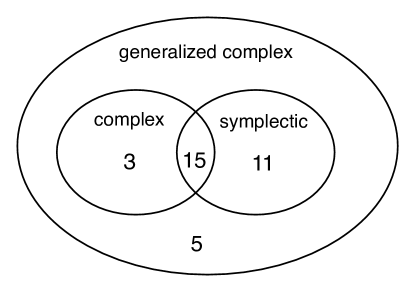
We adopt a similar format for presenting compact (algebraic) solvmanifolds which are collected in Table 5. A word of caution is due here. As already mentioned, for the nilmanifolds, the de Rham cohomology is isomorphic to the Lie algebra cohomology ${\cal G}$ [38]. This is no longer the case for generic solvmanifolds. Thus the first of the integers labeling each entry in Table 5 refers to the dimension of the first cohomology on the complex of the left–invariant forms.

In table 4, the next four columns (taken from [21]) tell about the types of the closed pure spinors, i. e. some underlying integrable structure, admitted by the given nilmanifold. If such a spinor exists, it is marked by a symbol $\surd$. The construction of the most general closed pure spinor of the given type is not hard, and examples are given in the text. In order to compare to Figure 1, we can count the number of $\surd$ in each column and confirm the existence of 18 closed type 3 pure spinors (i.s. integrable complex structure) and 26 type 0 (i.e. integrable symplectic structure). Note that we talk here only about the individual pure spinors — two closed pure spinors of different types for a given manifold are not compatible and do not define a metric. In particular the 15 nilmanifolds that have both closed type 3 and 0, do not have a metric of special holonomy to go along with these. Finally, we see that there are 5 cases where there are no closed type 0 or 3 pure spinors. These were the cases shown to admit a generalized complex structure in [21], i.e. either type 1 or type 2 closed pure spinor.

The last five columns (in both Tables) give the possible involutions compatible of the algebras. We actually only considered involutions that act with $\pm$ on the basis of one–forms $e^{a}$. All other involutions we found were related to these by changes of coordinates. It is possible that more involutions exist. With this in mind, the action of the involution on the one–forms $\sigma(e^{i})=\pm e^{i}$ can be characterized, in each case, by a certain number of independent signs. For example, considering the manifold 2.1 of Table 4, it is not hard to see that choosing the sign of $e^{1}$ and $e^{2}$ determines all the others. For example, since $f^{3}_{12}=1$, the sign ${\rm sign}(e^{3})$ is forced to be equal to the product ${\rm sign}(e^{1})\times{\rm sign}(e^{2})$. The rest of the signs are determined by the sign of these two. The manifold 2.3, on the other hand, is more restrictive due to the extra condition ${\rm sign}(e^{1})\times{\rm sign}(e^{5})={\rm sign}(e^{2})\times{\rm sign}(e^{3})$. This leaves us with a single one–form whose sign can be chosen independently from the others. Of course when we realize all the possibilities, we are going to get different assignments of $+$ and $-$ signs which give us all the admissible orientifold planes. Clearly the case of six pluses is always allowed, while six minus signs are never allowed other than for zero structure constants, i. e. $T^{6}$. Thus it is not hard to see that if we sum the number of possible involutions for each manifold, the total is always $2^{n}-1$, where $n$ is the number of independent signs and we have subtracted one for the all-plus case which corresponds to an O9. The only exception to this is $T^{6}$, where to the total on the last line of the Table 4 we should add 1 for the O3–plane in order to get all of the 63 allowed orientifold planes.

Some additional explanation is due for the second column in Table 5. The criterion in [40] to check that a Lie group $G$ with given structure constants can be made compact by quotienting by a subgroup $\Gamma$ assumes that $G$ be algebraic (as explained in 2.2). As checking this hypothesis might be tricky, we have first applied Saito’s criterion to all the solvable algebras in [32] and [33]. All the ones that passed the test are given in Table 5. Then, we have tried to check the algebraic hypothesis on each case of this restricted list. We have checked this by first explicitly finding by hand a faithful (one–to–one) $n$–dimensional (for some $n$) representation for $G$ in each case (the adjoint representation has usually a kernel and hence cannot be used; we have found the representations by trial and error). Given the representation, we have seen if the resulting subgroup of Gl$(n,\mathbb{R})$ could be described by polynomial equations. We denote this by a “${\rm yes}$” in the second column of the table. The ones for which this symbol is absent are still listed, because there might be another representation, which we have not found, in which $G$ is actually described by polynomial equations.

$n$	Nilmanifold class	T3	T2	T1	T0	O4	O5	O6	O7	O8
2.1	$(0,0,12,13,14,15)$	–	–	$\surd$	$\surd$	1	35	246	–	–
2.2	$(0,0,12,13,14,34+52)$	–	–	$\surd$	–	–	35;16;24	–	–	–
2.3	$(0,0,12,13,14,23+15)$	–	–	$\surd$	$\surd$	–	35	–	–	–
2.4	$(0,0,12,13,23,14)$	–	–	–	$\surd$	–	36;15;24	–	–	–
2.5	$(0,0,12,13,23,14-25)$	–	–	–	$\surd$	–	36;15;24	–	–	–
2.6	$(0,0,12,13,23,14+25)$	$\surd$	$\surd$	$\surd$	$\surd$	–	36;15;24	–	–	–
2.7	$(0,0,12,13,14+23,34+52)$	–	–	$\surd$	–	–	24	–	–	–
2.8	$(0,0,12,13,14+23,24+15)$	–	–	$\surd$	$\surd$	–	–	246	–	–
3.1	$(0,0,0,12,13,14+35)$	–	$\surd$	$\surd$	–	–	34;45	–	1246	–
3.2	$(0,0,0,12,13,14+23)$	$\surd$	$\surd$	$\surd$	$\surd$	–	34	135;236	–	–
3.3	$(0,0,0,12,13,24)$	$\surd$	$\surd$	$\surd$	$\surd$	–	23;16;25;34;45	–	1246;1356	–
3.4	$(0,0,0,12,13,14)$	$\surd$	$\surd$	$\surd$	$\surd$	1	34;45	236;135;256	1246	–
3.5	$(0,0,0,12,13,23)$	$\surd$	$\surd$	$\surd$	$\surd$	–	16;25;34	124;135;236;456	–	–
3.6	$(0,0,0,12,14,15+23)$	–	–	$\surd$	$\surd$	–	46;13;25	–	–	–
3.7	$(0,0,0,12,14,15+23+24)$	–	–	$\surd$	$\surd$	–	25	–	–	–
3.8	$(0,0,0,12,14,15+24)$	–	–	$\surd$	$\surd$	–	25	235	–	$\bot$3
3.9	$(0,0,0,12,14,15)$	–	–	$\surd$	$\surd$	1	46;13;25	235;346	–	$\bot$3
3.10	$(0,0,0,12,14,24)$	$\surd$	$\surd$	$\surd$	–	4	16;25;34	136;235	–	$\bot$3
3.11	$(0,0,0,12,14,13+42)$	$\surd$	–	$\surd$	$\surd$	–	34	136;235	–	–
3.12	$(0,0,0,12,14,23+24)$	$\surd$	–	$\surd$	$\surd$	–	34;25;16	-	–	–
3.13	$(0,0,0,12,23,14+35)$	–	$\surd$	$\surd$	–	–	13;15;26;34;45	–	1246;2356	–
3.14	$(0,0,0,12,23,14-35)$	$\surd$	$\surd$	$\surd$	–	–	13;15;26;34;45	–	1246;2356	–
3.15	$(0,0,0,12,14-23,15+34)$	–	$\surd$	$\surd$	$\surd$	–	13	235;346	–	–
3.16	$(0,0,0,12,14+23,13+42)$	$\surd$	$\surd$	$\surd$	$\surd$	–	34	136;235	–	–
4.1	$(0,0,0,0,12,15+34)$	–	$\surd$	$\surd$	–	–	35;45;26;13;14	–	1256;2346	–
4.2	$(0,0,0,0,12,15)$	–	$\surd$	$\surd$	$\surd$	1;5	26;13;14;35;45	134;236;246;345	1256;2346	$\bot$:3;4
4.3	$(0,0,0,0,12,14+25)$	$\surd$	$\surd$	$\surd$	$\surd$	–	24;45	146;234;345	1346	$\bot$3
4.4	$(0,0,0,0,12,14+23)$	$\surd$	$\surd$	$\surd$	$\surd$	–	56;13;24	125;146;236;345	–	–
4.5	$(0,0,0,0,12,34)$	$\surd$	$\surd$	$\surd$	$\surd$	–	56;16;26;14;13 23;24;35;45	–	1235;1245;1256 1346;2346;3456	–
4.6	$(0,0,0,0,12,13)$	$\surd$	$\surd$	$\surd$	$\surd$	1	56;14;26;35;23	234;125;136 246;345;456	1245;1346	$\bot$4
4.7	($0,0,0,0,13+42,14+23)$	$\surd$	$\surd$	$\surd$	$\surd$	–	56;12;34	135;146;236;245	–	–
5.1	$(0,0,0,0,0,12+34)$	$\surd$	$\surd$	$\surd$	–	6	56;13;14;23;24	126;346;135;145 235; 245	1256;3456	$\bot$5
5.2	$(0,0,0,0,0,12)$	$\surd$	$\surd$	$\surd$	$\surd$	1;2;6	56;13;14;23;24 36;46;15;25	126;346;135;145 235;245;356;456 134;234	1236;1246;1256 1345;2345;3456	$\bot$:3;4;5
6.1	$(0,0,0,0,0,0)$	$\surd$	$\surd$	$\surd$	$\surd$	any (6)	any (15)	any (20)	any (15)	any (6)

Table 4: Six–dimensional nilmanifolds.

$s$	Alg.?	Solvmanifold class	O4	O5	O6	O7	O8
1.1	${\rm yes}\ \forall\alpha\in\mathbb{Z}$	$(23,-36,26,-\alpha 56,\alpha 46,0)$	-	16,24,25,34,35	–	1236,1456	–
1.2		$(24+35,-36,26,-56,46,0)$	-	16,25,34	124,135,236,456	–	–
2.1		$(23,0,26,-56,46,0)$	-	16,24,25,34,35	–	1236,1456	–
2.2	${\rm yes}$	$(35-26,45+16,-46,36,0,0)$	-	14,23,56	126,135,245,346	–	–
2.3	${\rm yes}$	$(24+35,0,-56,0,36,0)$	-	16,23,25,34,45	–	1246,1356	–
2.4	${\rm yes}$	(23,-13,0,56,-46,0)	–	14,15,16,24,25 26,34,35,36	–	1234,1235,1236 1456,2456,3456	–
2.5	${\rm yes}\ \forall\alpha\in\mathbb{Z}$	$(25,-15,\alpha 45,-\alpha 35,0,0)$	5	13,14,23,24,56	125,136,146,236,246,345	3456, 1256	$\bot$ 6
2.6		(25+35,-15+45,45,-35,0,0)	5	14,23,56	146,236	–	$\bot$ 6
3.1	${\rm yes}$	(23,-13,0,56,0,0)	–	14,15,16,24,25 26,34,35,36	–	1234,1235,1236 1456,2456,3456	–
3.2	${\rm yes}$	(23,34,-24,0,0,0)	2, 3	14,25,26,35,36	146,145,256,356	1234, 1456	$\bot$:5,6
3.3		(25,0,45,-35,0,0)	5	13,14,23,24,56	125,136,146,236,246,345	3456, 1256	$\bot$6
3.4		$(23+45,-35,25,0,0,0)$	–	24,34	145,246,346	1456	$\bot$ 6
4.1	${\rm yes}$	$(23,-13,0,0,0,0)$	1;2;3	14,15,16,24,25, 26,34,35,36	123,145,156,346,256 245,356,345,146,246	1236,1234,1235 1456,2456,3456	$\bot$:4,5,6

Table 5: Six–dimensional compact solvmanifolds which are possibly algebraic.

In both Tables we label the manifolds by the dimension of the first cohomology on the space of left–invariant forms, and the position they occupy in the Table. A $\surd$ indicates that the manifold admits a closed pure spinor of the given type (T3=type 3). We indicate the allowed O4,O5, O6 and O7–planes by giving its parallel directions, and O8–planes by giving the transverse ones. The symbol ‘-’ denotes nonexistence of either a pure spinor or an O–plane. In Table 5, only the ones with a ”${\rm yes}$” in the second column are established as compact solvmanifolds; the other ones might or might not be. Also, we do not consider non–algebraic compact solvmanifolds. Notice that s 3.2 is actually obtained by setting $\alpha=0$ in s 1.1, and likewise s 4.1 is obtained by setting $\alpha=0$ in s 2.5. Given that doing this changes the Lie algebra cohomology (the cohomology computed on the left–invariant forms), we have decided to list them separately.

Appendix C Orientifold projections and pure spinor equations

In this Appendix we give the form of the supersymmetry equations (4.2) and (4.3) for the different orientifold projections in IIA and IIB in the cases of type0–type3 spinors (3.73) and type1–type2 (3.79), subject to the rescaling Ansatz supposing the rescalings (5.2):

$$e^{\alpha}_{+}=e^{A}\tilde{e}^{\alpha}_{+}\,\qquad e^{i}_{-}=e^{-A}\tilde{e}^{i}_{-}\ .$$

We also give the most general form of pure spinors in terms of the 1-forms $e^{\alpha},e^{i}$ transforming under the involution as $\sigma(e^{\alpha})=e^{\alpha}$, $\sigma(e^{i})=-e^{i}$ and the moduli of the manifolds.

C.1 IIB: O5 orientifolds

For type3–type0 pure spinors, (3.73 the O5 projection sets $a=b$. Inserting the explicit expressions for the spinors in the supersymmetry variations (4.2),(4.3) with $\Phi_{1}=\Phi_{-}$, $\Phi_{2}=\Phi_{+}$, we obtain

$$e^{\phi}=g_{s}e^{2A}$$

$$d(e^{A}\Omega_{3})=0$$

$$dJ^{2}=0$$

$$d(e^{2A}J)=g_{s}e^{4A}*F_{3}$$

$$H=0\ ,$$ (C.1)

where $g_{s}$ in the first equation is an integration constant, that we take to be the large volume limit ($A=0$) of $e^{\phi}$. In this case, these equations actually follow from (4.2), (4.3), without assuming (5.2). The most general $\Omega_{3}$ compatible with the O5 projection (which leaves it invariant) is

$$\Omega_{3}\equiv z^{1}\wedge z^{2}\wedge z^{3}=(e^{1}_{-}+i\tau^{1}e^{3}_{-}+i\tau^{2}e^{4}_{-})\wedge(e^{2}_{-}+i\tau^{3}e^{3}_{-}+i\tau^{4}e^{4}_{-})\wedge(e^{1}_{+}+i\tau^{+}e^{2}_{+})\ .$$ (C.2)

where $\tau^{+},\tau^{1},\ldots,\tau^{4}$ are complex constants and by definition $z^{i}$ are the holomorphic 1-forms. The most general fundamental 2-form compatible with $\Omega_{3}$ (i. e., satisfying (3.75)) is

$$J=\frac{i}{2}\left(t_{1}\ z^{1}\wedge{\bar{z}}^{1}+t_{2}\ z^{2}\wedge{\bar{z}}^{2}+b\ z^{1}\wedge{\bar{z}}^{2}-\bar{b}\ {\bar{z}}^{1}\wedge z^{2}+t_{3}\ z^{3}\wedge{\bar{z}}^{3}\right)\equiv J_{--}+J_{++}$$ (C.3)

where $t_{i}$ are real and $b$ is complex. The normalization condition (3.75) requires $t_{3}(t_{1}t_{2}-|b|^{2})=1$.

We now turn to the discussion of the hybrid of SU(2) structure. Inserting the type 1-type 2 pure spinors of Table 2 in eqs (4.2), (4.3), we get the following system

$$e^{\phi}=g_{s}e^{2A}$$ (C.4)

$$d(e^{A}\Omega_{1})=0$$

$$\Omega_{1}\wedge dj=-i\ \Omega_{1}\wedge H$$

$$d(e^{2A}{{\rm{Re}}}\Omega_{2})=-g_{s}e^{4A}*F_{3}$$

$$d({{\rm{Im}}}\Omega_{2})=0$$

$$i\,dA\wedge\,{\rm{Re}}\Omega_{2}\wedge\Omega_{1}\wedge\bar{\Omega}_{1}-\frac{1}{2}H\wedge{\rm{Im}}\Omega_{2}=-\frac{ig_{s}}{4}e^{2A}*F_{3}\wedge\Omega_{1}\wedge\bar{\Omega}_{1}$$

$$\frac{1}{2}H\wedge{{\rm{Re}}}\Omega_{2}=\frac{g_{s}}{2}e^{2A}*F_{1}$$

The transformation properties of the pure spinors and $H$ under the orientifold projection are given in Table 2. These imply

$$\Omega_{1} \equiv z^{3}=\tau^{-}_{i}e^{i}_{-}$$

$$\Omega_{2} \equiv z^{1}\wedge z^{2}=(e^{1}_{+}+i\tau^{1}_{i}e^{i}_{-})\wedge(e^{2}_{+}+i\tau^{2}_{i}e^{i}_{-})$$

$$j = \frac{i}{2}\left(t_{1}z^{1}\wedge\bar{z}^{1}+t_{2}z^{2}\wedge\bar{z}^{2}+b(z^{1}\wedge\bar{z}^{2}-\bar{z}^{1}\wedge z^{2})\right)$$

$$H = h_{i}\ e^{i}_{-}\wedge e^{1}_{+}\wedge e^{2}_{+}+h^{\prime}_{i}\ \epsilon^{ijkl}\ e^{j}_{-}\wedge e^{k}_{-}\wedge e^{l}_{-}\ ,$$ (C.5)

where a sum over $i,j,k,l=1,\ldots,4$ is understood. In these equations $\tau^{-}_{i}$ are complex, while $\tau^{1}_{i}$, $\tau^{2}_{i}$ are real, which means there are 8 complex structure moduli in all. On the other hand, $t_{1}$, $t_{2}$ and $b$ are all real, the same as $h_{i}$, $h^{\prime}_{i}$.

The volume is given by

$${\rm vol}=\sqrt{\tilde{g}}\,e^{1}_{-}\wedge e^{2}_{-}\wedge e^{3}_{-}\wedge e^{4}_{-}\wedge e^{1}_{+}\wedge e^{2}_{+}=-8ie^{-2A}\left<\Phi_{\pm},\bar{\Phi}_{\pm}\right>=\frac{i}{8}\Omega_{2}\wedge\bar{\Omega}_{2}\wedge\Omega_{1}\wedge\bar{\Omega}_{1}$$ (C.6)

where the normalization condition $\left<\bar{\Phi}_{+},\Phi_{+}\right>=\left<\bar{\Phi}_{-},\Phi_{-}\right>$ requires $\Omega_{2}\wedge\bar{\Omega}_{2}=2j^{2}$, or in other words $(t_{1}t_{2}-|b|^{2})=1$.

C.2 IIB: O7 orientifolds

For the O7 case, the supersymmetry equations (4.2) and (4.3) for type0-type3 become

$$e^{\phi} = g_{s}e^{4A}$$

$$d(e^{-A}\Omega_{3}) = 0$$

$$d(e^{-2A}J) = 0$$

$$d(J^{2}) = -2\,g_{s}\,e^{4A}*F_{1}$$

$$H = e^{4A}\,g_{s}\,*F_{3}$$

$$H\wedge\Omega_{3} = H\wedge J=0$$ (C.7)

and the general form of t $\Omega_{3}$ and $J$ compatible with the orientifold projection is

$$\Omega_{3} = (e^{1}_{+}+i\tau^{1}e^{3}_{+}+i\tau^{2}e^{4}_{+})\wedge(e^{2}_{+}+i\tau^{3}e^{3}_{+}+i\tau^{4}e^{4}_{+})\wedge(e^{1}_{-}+i\tau^{-}e^{2}_{-})$$

$$J = \frac{i}{2}\left(t_{1}\ z^{1}\wedge{\bar{z}}^{1}+t_{2}\ z^{2}\wedge{\bar{z}}^{2}+b\ z^{1}\wedge{\bar{z}}^{2}-\bar{b}\ {\bar{z}}^{1}\wedge z^{2}+t_{3}\ z^{3}\wedge{\bar{z}}^{3}\right)\ .$$ (C.8)

In these expressions, all $\tau$’s as well as $b$ are complex, while $t_{i}$ are real.

For type1–type 2 the supersymmetry equations are

$$e^{\phi} = g_{s}e^{4A}$$

$$d(e^{-A}\Omega_{1}) = 0$$

$$\Omega_{1}\wedge dj = -i\ \Omega_{1}\wedge H$$

$$d(e^{-2A}{\rm{Re}}\Omega_{2}) = 0$$

$$d({\rm{Im}}\Omega_{2}) = -g_{s}\,e^{4A}*F_{3}$$

$$-2i\,dA\wedge\,{\rm{Re}}\Omega_{2}\wedge\Omega_{1}\wedge\bar{\Omega}_{1}-H\wedge{\rm{Im}}\Omega_{2} = g_{s}\,e^{4A}*F_{1}$$

$$2\,iH\wedge{\rm{Re}}\Omega_{2} = -2\,i\,g_{s}\,e^{4A}*F_{3}\,\Omega_{1}\wedge\bar{\Omega}_{1}$$ (C.9)

The transformations of the spinors imply

$$\Omega_{1} \equiv z^{3}=\tau^{+}_{\alpha}e^{\alpha}_{+}$$

$$\Omega_{2} \equiv z^{1}\wedge z^{2}=(e^{1}_{-}+i\tau^{1}_{i}e^{i}_{+})\wedge(e^{2}_{-}+i\tau^{2}_{i}e^{i}_{+})$$

$$j = \frac{i}{2}\left(t_{1}z^{1}\wedge\bar{z}^{1}+t_{2}z^{2}\wedge\bar{z}^{2}+b\,(z^{1}\wedge\bar{z}^{2}-\bar{z}^{1}\wedge z^{2})\right)$$

$$H = h_{1i}\ e^{i}_{-}\wedge e^{1}_{+}\wedge e^{2}_{+}+h_{2i}\ e^{i}_{-}\wedge e^{1}_{+}\wedge e^{3}_{+}+h_{3i}\ e^{i}_{-}\wedge e^{1}_{+}\wedge e^{4}_{+}+$$ (C.10)

$$h_{4i}\ e^{i}_{-}\wedge e^{2}_{+}\wedge e^{3}_{+}+h_{5i}\ e^{i}_{-}\wedge e^{2}_{+}\wedge e^{4}_{+}+h_{6i}\ e^{i}_{-}\wedge e^{3}_{+}\wedge e^{4}_{+}$$

where $\tau_{i}^{+}$ are complex, while all the rest are real.

C.3 IIA: O6 orientifolds

We start with the SU(3) structure case. For type3-type 0 spinors corresponding to O6, eqs. (4.2) and (4.3) become

$$e^{\phi} = g_{s}e^{3A}$$

$$H = 0$$

$$dJ = 0$$

$$d(e^{-A}{\rm{Re}}\Omega_{3}) = 0$$

$$d(e^{A}{\rm{Im}}\Omega_{3}) = \,-g_{s}\,e^{4A}*F_{2}\ .$$ (C.11)

The most general spinors compatible with the orientifold projection are

$$\Omega_{3} \equiv z^{1}\wedge z^{2}\wedge z^{3}=(e^{1}_{-}+i\tau^{1}_{\alpha}e^{\alpha}_{+})\wedge(e^{2}_{-}+i\tau^{2}_{\alpha}e^{\alpha}_{+})\wedge(e^{3}_{-}+i\tau^{3}_{\alpha}e^{\alpha}_{+})$$

$$J = \frac{i}{2}\sum_{i=1}^{3}t_{i}\ z^{i}\wedge{\bar{z}}^{i}+{\rm{Im}}\left(b_{1}\ z^{2}\wedge{\bar{z}}^{3}+b_{2}\ z^{3}\wedge{\bar{z}}^{1}+b_{3}\ z^{1}\wedge{\bar{z}}^{2}\right)$$ (C.12)

where all $\tau^{i}_{j}$, $a_{i}$ and $b_{i}$ are real.

For type1 – type 2 spinors, or in other words for SU(2) structure, and an O6 projections we get the following equations

$$e^{\phi} = g_{s}e^{3A}$$

$$d(\Omega_{2}) = 0$$

$$d(\Omega_{1}\wedge\bar{\Omega}_{1})\wedge\Omega_{2} = 2\,H\wedge\Omega_{2}$$

$$d(e^{-A}j\wedge{\rm{Re}}\Omega_{1}) = -e^{-A}H\wedge{\rm{Im}}\Omega_{1}$$

$$d(e^{A}{\rm{Re}}\Omega_{1}) = \,g_{s}\,e^{4A}*F_{4}$$

$$d(e^{A}j\wedge{\rm{Im}}\Omega_{1}) = e^{A}H\wedge{\rm{Re}}\Omega_{1}-\,g_{s}\,e^{4A}*F_{2}$$ (C.13)

The general spinor for this case are

$$\Omega_{1} \equiv z^{3}=\tau^{-}_{i}e^{i}_{-}+i\tau^{+}_{\alpha}e^{\alpha}_{+}$$

$$\Omega_{2} \equiv z^{1}\wedge z^{2}=(\tau^{1}_{\alpha}e^{\alpha}_{+})\wedge(\tau^{2}_{i}e^{i}_{-})$$

$$j = \frac{i}{2}\left(t_{1}\,z^{1}\wedge\bar{z}^{1}+t_{2}\,z^{2}\wedge\bar{z}^{2}\right)$$

$$H = h_{-}\ e^{1}_{-}\wedge e^{2}_{-}\wedge e^{3}_{-}+h_{i\alpha}\ \epsilon^{\alpha\beta\gamma}\ e^{i}_{-}\wedge e^{\beta}_{+}\wedge e^{\gamma}_{+}\ .$$ (C.14)

In these expressions, $\tau^{1,2}_{\alpha,i}$ are complex, while $\tau^{\pm}_{\alpha,i}$, $t_{i}$ and $h$’s are real.

C.4 IIA: O4 and O8 orientifolds

The O4 and O8 projections do not allow SU(3) structure. Thus we only give the supersymmetry variations for the type1–type2 pure spinors

$$e^{\phi}=g_{s}e^{A}\,,$$

$$d(e^{A}v^{\prime})=0\,,$$

$$d(e^{2A}\Omega_{2})=0\,,$$

$$d(e^{A}v\wedge j)=-e^{A}H\wedge v^{\prime}\,,$$ (C.15)

$${\rm Re}\Omega_{2}\wedge d(v\wedge v^{\prime})=-H\wedge{\rm Im}\Omega_{2}\,,$$

$${\rm Im}\Omega_{2}\wedge d(v\wedge v^{\prime})=H\wedge{\rm Re}\Omega_{2}\,,$$

$$v^{\prime}\wedge j\wedge dj=-H\wedge v\wedge j\,,$$

$$d(e^{3A}v)=\,-g_{s}\,e^{4A}*F_{4}\,,$$

$$d(e^{3A}v^{\prime}\wedge j)=e^{3A}H\wedge v+\,g_{s}\,e^{4A}*F_{2}\,,$$

$$d(e^{3A}v\wedge j\wedge j)=-2e^{3A}H\wedge v^{\prime}\wedge j+2\,g_{s}\,e^{4A}*F_{0}\,.$$ (C.16)

The general pure spinors compatible with an O4 and the NS flux are

$$\Omega_{1} \equiv z^{3}=e_{+}+i\tau^{3}_{i}e^{i}_{-}$$

$$\Omega_{2} \equiv z^{1}\wedge z^{2}=(\tau^{1}_{i}e^{i}_{-})\wedge(\tau^{2}_{i}e^{i}_{-})$$

$$j = \frac{i}{2}\left(t_{1}\,z^{1}\wedge\bar{z}^{1}+t_{2}\,z^{2}\wedge\bar{z}^{2}+b\ z^{1}\wedge{\bar{z}}^{2}-\bar{b}\ {\bar{z}}^{1}\wedge z^{2}\right)$$

$$H = h_{ij}\epsilon^{ijklm}e^{k}_{-}\wedge e^{l}_{-}\wedge e^{m}_{-}$$ (C.17)

where $\tau^{3}_{i}$, $t_{i}$ are real, while $\tau^{1,2}_{i}$ and $b$ are complex, and we should bear in mind that $\Omega_{1}=v+iv^{\prime}$. The spinors compatible with an O8 are

$$\Omega_{1} \equiv z^{3}=\tau^{3}_{\alpha}e^{i}_{\alpha}+ie_{-}$$

$$\Omega_{2} \equiv z^{1}\wedge z^{2}=(\tau^{1}_{\alpha}e^{\alpha}_{+})\wedge(\tau^{2}_{\alpha}e^{\alpha}_{+})$$

$$j = \frac{i}{2}\left(t_{1}\,z^{1}\wedge\bar{z}^{1}+t_{2}\,z^{2}\wedge\bar{z}^{2}+b\ z^{1}\wedge{\bar{z}}^{2}-\bar{b}\ {\bar{z}}^{1}\wedge z^{2}\right)$$

$$H = h_{ij}e^{-}\wedge e^{i}_{+}\wedge e^{j}_{+}$$ (C.18)

where $\tau^{3}_{i}$, $t_{i}$ are real, while $\tau^{1,2}_{i}$ and $b$ are complex.

In the presence of O8–planes alone, the only flux allowed is $F_{0}$, and it comes purely from a derivative of the warp factor. In the large volume limit, there are no RR fluxes and therefore the manifolds are generalized Kähler. This is similar to the situation for O7 projection. However, the pure spinors for O8 have a very nonsymmetric expression, and looking for two closed pure spinors of this form turns out to be much more involved. We have checked that there are no solutions among the compact solvable not nilpotent algebras, but the possibility of finding a solution among the nilpotent ones is not ruled out.

References

- [1] M. Graña, “Flux compactifications in string theory: A comprehensive review,” Phys. Rept. 423 (2006) 91 [arXiv:hep-th/0509003].
- [2] S. Kachru, M. B. Schulz, P. K. Tripathy and S. P. Trivedi, “New supersymmetric string compactifications,” JHEP 0303, 061 (2003) [arXiv:hep-th/0211182].
- [3] G. Villadoro and F. Zwirner, “The minimal N = 4 no-scale model from generalized dimensional reduction,” JHEP 0407 (2004) 055 [arXiv:hep-th/0406185].
- [4] J. P. Derendinger, C. Kounnas, P. M. Petropoulos and F. Zwirner, “Superpotentials in IIA compactifications with general fluxes,” Nucl. Phys. B 715 (2005) 211 [arXiv:hep-th/0411276].
- [5] G. Dall’Agata and S. Ferrara, “Gauged supergravity algebras from twisted tori compactifications with fluxes,” Nucl. Phys. B 717 (2005) 223 [arXiv:hep-th/0502066].
- [6] C. M. Hull and R. A. Reid-Edwards, “Flux compactifications of string theory on twisted tori,” arXiv:hep-th/0503114.
- [7] G. Dall’Agata, R. D’Auria and S. Ferrara, “Compactifications on twisted tori with fluxes and free differential algebras,” Phys. Lett. B 619 (2005) 149 [arXiv:hep-th/0503122].
- [8] G. Villadoro and F. Zwirner, “N = 1 effective potential from dual type-IIA D6/O6 orientifolds with general fluxes,” JHEP 0506 (2005) 047 [arXiv:hep-th/0503169].
- [9] O. DeWolfe, A. Giryavets, S. Kachru and W. Taylor, “Type IIA moduli stabilization,” JHEP 0507 (2005) 066 [arXiv:hep-th/0505160].
- [10] P. G. Camara, A. Font and L. E. Ibanez, “Fluxes, moduli fixing and MSSM-like vacua in a simple IIA orientifold,” JHEP 0509 (2005) 013 [arXiv:hep-th/0506066].
- [11] G. Dall’Agata and N. Prezas, “Scherk-Schwarz reduction of M-theory on G2-manifolds with fluxes,” JHEP 0510, 103 (2005) [arXiv:hep-th/0509052].
- [12] R. D’Auria, S. Ferrara and M. Trigiante, “Supersymmetric completion of M-theory 4D-gauge algebra from twisted tori and fluxes,” JHEP 0601, 081 (2006) [arXiv:hep-th/0511158].
- [13] J. P. Derendinger, C. Kounnas and P. M. Petropoulos, “Gaugino condensates and fluxes in N = 1 effective superpotentials,” Nucl. Phys. B 747 (2006) 190 [arXiv:hep-th/0601005].
- [14] P. Fre’ and M. Trigiante, “Twisted tori and fluxes: A no go theorem for Lie groups of weak G(2) holonomy,” arXiv:hep-th/0603011.
- [15] C. M. Hull and R. A. Reid-Edwards, “Flux Compactifications of M-Theory on Twisted Tori,” arXiv:hep-th/0603094.
- [16] G. Aldazabal, P. G. Camara, A. Font and L. E. Ibanez, “More dual fluxes and moduli fixing,” JHEP 0605 (2006) 070 [arXiv:hep-th/0602089].
- [17] N. Hitchin, “Generalized Calabi-Yau manifolds,” math.DG/0107101.
- [18] M. Gualtieri, “Generalized complex geometry,” Oxford University DPhil thesis, math.DG/0401221.
- [19] M. Graña, R. Minasian, M. Petrini and A. Tomasiello, “Supersymmetric backgrounds from generalized Calabi-Yau manifolds,” JHEP 0408, 046 (2004) [arXiv:hep-th/0406137].
- [20] M. Graña, R. Minasian, M. Petrini and A. Tomasiello, “Generalized structures of N = 1 vacua,” arXiv:hep-th/0505212.
- [21] G. Cavalcanti and M. Gualtieri, “Generalized complex structures on nilmanifolds,” J. Symplectic Geom. 2 393 (2004) [math.DG/0404451].
- [22] L. Andrianopoli, R. D’Auria, S. Ferrara, P. Fre and M. Trigiante, “R-R scalars, U-duality and solvable Lie algebras,” Nucl. Phys. B 496, 617 (1997) [arXiv:hep-th/9611014].
- [23] L. Andrianopoli, R. D’Auria, S. Ferrara, P. Fre, R. Minasian and M. Trigiante, “Solvable Lie algebras in type IIA, type IIB and M theories,” Nucl. Phys. B 493, 249 (1997) [arXiv:hep-th/9612202].
- [24] F. Cordaro, P. Fre, L. Gualtieri, P. Termonia and M. Trigiante, “N = 8 gaugings revisited: An exhaustive classification,” Nucl. Phys. B 532, 245 (1998) [arXiv:hep-th/9804056].
- [25] L. Andrianopoli, R. D’Auria, S. Ferrara and M. A. Lledo, “Gauging of flat groups in four–dimensional supergravity,” JHEP 0207, 010 (2002) [arXiv:hep-th/0203206].
- [26] M. B. Schulz, “Superstring orientifolds with torsion: O5 orientifolds of torus fibrations and their massless spectra,” Fortsch. Phys. 52 (2004) 963 [arXiv:hep-th/0406001].
- [27] B. S. Acharya, F. Benini and R. Valandro, “Fixing moduli in exact type IIA flux vacua,” arXiv:hep-th/0607223.
- [28] J. P. Gauntlett, D. Martelli, S. Pakis and D. Waldram, “G-structures and wrapped NS5-branes,” Commun. Math. Phys. 247, 421 (2004) [arXiv:hep-th/0205050].
-
[29]
M. Grana and J. Polchinski,
“Supersymmetric three-form flux perturbations on AdS(5),”
Phys. Rev. D 63, 026001 (2001)
[arXiv:hep-th/0009211].
S. S. Gubser, “Supersymmetry and F-theory realization of the deformed conifold with three-form flux,” arXiv:hep-th/0010010. - [30] S. B. Giddings, S. Kachru and J. Polchinski, “Hierarchies from fluxes in string compactifications,” Phys. Rev. D 66, 106006 (2002) [arXiv:hep-th/0105097].
[31]
K. Becker and M. Becker,
“M-Theory on Eight-Manifolds,”
Nucl. Phys. B 477, 155 (1996)
[arXiv:hep-th/9605053].
K. Dasgupta, G. Rajesh and S. Sethi, “M theory, orientifolds and G-flux,” JHEP 9908, 023 (1999) [arXiv:hep-th/9908088]. - [32] P. Turkowski, “Solvable Lie algebras of dimension six,” J. Math. Phys. 31, 1344 (1990).
- [33] G. M. Mubarakzjanov, “Classification of Solvable Lie Algebras of Sixth Order with a NonNilpotent Basis Element,” Izv. Vysš. Učehn. Zaved. 35 104 (1963).
- [34] V. V. Morozov, “Classification of nilpotent Lie algebras of sixth order,” Izv. Vysš. Učebn. Zaved. 4 (5), 161(1958).
- [35] L. Magnin, “Sur les algèbres de Lie nilpotentes de dimension ,” J. Geom. Phys. 3 , 119 (1986) .
- [36] J. Scherk and J. H. Schwarz, “How To Get Masses From Extra Dimensions,” Nucl. Phys. B 153 (1979) 61.
- [37] L. Auslander, “An exposition of the structure of solvmanifolds. I. Algebraic theory,” Bull. Amer. Math. Soc. 79 227 (1973).
- [38] K. Nomizu, “On the cohomology of compact homogeneous spaces of nilpotent Lie groups,” Ann. of Math. (2) 59, 531 (1954).
- [39] A. I. Malcev, “On a class of homogeneous spaces,” Amer. Math. Soc. Translation 39 (1951).
- [40] M. Saito, “Sous-groupes discrets des groupes resolubles,” Am. J. Math. 83, 369(1961).
- [41] G. M. Mubarakzjanov, “On solvable Lie algebras,” Izv. Vysš. Učehn. Zaved. 32, 114 (1963).
- [42] C. Bock, “On Low-Dimensional Solvmanifolds,” arXiv:0903.2926[math.SG].
- [43] S. S. Haque, G. Shiu, B. Underwood and T. Van Riet, “Minimal simple de Sitter solutions,” Phys. Rev. D 79 (2009) 086005 [arXiv:0810.5328 [hep-th]].
- [44] L. Auslander and R. H. Szczarba, “Characteristic classes of compact solvmanifolds,” Ann. of Math. (1) 76, 531 (1962).
- [45] D. V. Alekseevskii and B. N. Kimel’fel’d, “Structure of homogeneous Riemannian spaces with zero Ricci curvature,” Funct. Anal. Appl. 9 , 97 (1975).
- [46] F. Witt, “Special metric structures and closed forms,” arXiv:math.dg/0502443.
- [47] Y. Kosmann-Schwarzbach, “Derived brackets,” Lett. Math. Phys. 69 61 (2004) [math.DG/0312524].
- [48] N. Berkovits, “Super-Poincare covariant quantization of the superstring,” JHEP 0004 (2000) 018 [arXiv:hep-th/0001035].
- [49] C. Chevalley, The algebraic theory of spinors, Columbia University Perss, 1954.
- [50] S. Chiossi, S. Salamon, “The intrinsic torsion of and structures,” Differential geometry, Valencia, 2001, 115–133, World Sci. Publishing, River Edge, NJ, 2002.
- [51] A. Giveon, M. Porrati and E. Rabinovici, “Target space duality in string theory,” Phys. Rept. 244 (1994) 77 [arXiv:hep-th/9401139].
- [52] E. Bergshoeff, R. Kallosh, T. Ortin, D. Roest and A. Van Proeyen, “New formulations of D = 10 supersymmetry and D8 – O8 domain walls,” Class. Quant. Grav. 18 (2001) 3359 [arXiv:hep-th/0103233].
- [53] C. Jeschek and F. Witt, “Generalised G(2)-structures and type IIB superstrings,” JHEP 0503, 053 (2005) [arXiv:hep-th/0412280].
- [54] D. Lust and D. Tsimpis, “Supersymmetric AdS(4) compactifications of IIA supergravity,” JHEP 0502 (2005) 027 [arXiv:hep-th/0412250].
- [55] L. Martucci and P. Smyth, “Supersymmetric D–branes and calibrations on general N = 1 backgrounds,” JHEP 0511 (2005) 048 [arXiv:hep-th/0507099].
- [56] L. Martucci, “D–branes on general N = 1 backgrounds: Superpotentials and D-terms,” JHEP 0606 (2006) 033 [arXiv:hep-th/0602129].
- [57] C. Jeschek and F. Witt, ”Generalised geometries, constrained critical points and Ramond-Ramond fields”, arXiv:math.DG/0510131.
- [58] B. de Wit, D. J. Smit and N. D. Hari Dass, “Residual supersymmetry of compactified d=10 supergravity,” Nucl. Phys. B 283 (1987) 165.
- [59] J. M. Maldacena and C. Nuñez, “Supergravity description of field theories on curved manifolds and a no go theorem,” Int. J. Mod. Phys. A 16, 822 (2001) [arXiv:hep-th/0007018].
- [60] I. Benmachiche and T. W. Grimm, “Generalized N = 1 orientifold compactifications and the Hitchin functionals,” arXiv:hep-th/0602241.
- [61] T. W. Grimm and J. Louis, “The effective action of N = 1 Calabi-Yau orientifolds,” Nucl. Phys. B 699, 387 (2004) [arXiv:hep-th/0403067]; “The effective action of type IIA Calabi-Yau orientifolds,” Nucl. Phys. B 718, 153 (2005) [arXiv:hep-th/0412277].
- [62] P. Koerber and D. Tsimpis, “Supersymmetric sources, integrability and generalized–structure compactifications,” JHEP 0708 (2007) 082 [arXiv:0706.1244 [hep-th]].
- [63] J. Scherk and J. H. Schwarz, “How To Get Masses From Extra Dimensions,” Nucl. Phys. B 153, 61 (1979).
- [64] S. Hellerman, J. McGreevy, B. Williams, “Geometric Constructions of Nongeometric String Theories,” JHEP 0401 (2004) 024 [arXiv:hep-th/0208174].
- [65] D. Andriot, ”New supersymmetric flux vacua with intermediate SU(2) structure,” JHEP 0808 (2008) 096 [arXiv:0804.1769 [hep-th]].
- [66] S. Fidanza, R. Minasian and A. Tomasiello, “Mirror symmetric SU(3)-structure manifolds with NS fluxes,” Commun. Math. Phys. 254, 401 (2005) [arXiv:hep-th/0311122].
- [67] S. F. Hassan, “SO(d,d) transformations of Ramond-Ramond fields and space-time spinors,” Nucl. Phys. B 583 (2000) 431 [arXiv:hep-th/9912236].
- [68] E. Alvarez, L. Alvarez-Gaume, J. L. F. Barbon and Y. Lozano, “Some global aspects of duality in string theory,” Nucl. Phys. B 415 (1994) 71 [arXiv:hep-th/9309039].
- [69] M. J. Duff, H. Lu and C. N. Pope, “AdS(5) x S(5) untwisted,” Nucl. Phys. B 532 (1998) 181 [arXiv:hep-th/9803061].
- [70] P. Bouwknegt, J. Evslin and V. Mathai, “T–duality: Topology change from H-flux,” Commun. Math. Phys. 249 (2004) 383 [arXiv:hep-th/0306062].
- [71] A. Kapustin and D. Orlov, “Vertex algebras, mirror symmetry, and D–branes: The case of complex tori,” Commun. Math. Phys. 233 (2003) 79 [arXiv:hep-th/0010293].
- [72] A. Strominger, S. T. Yau and E. Zaslow, “Mirror symmetry is T–duality,” Nucl. Phys. B 479 (1996) 243 [arXiv:hep-th/9606040].
- [73] N. C. Leung, S. T. Yau and E. Zaslow, “From special Lagrangian to Hermitian-Yang-Mills via Fourier-Mukai transform,” Adv. Theor. Math. Phys. 4 (2002) 1319 [arXiv:math.dg/0005118].
- [74] P. Grange and R. Minasian, “Modified pure spinors and mirror symmetry,” Nucl. Phys. B 732 (2006) 366 [arXiv:hep-th/0412086].
- [75] M. Marino, R. Minasian, G. W. Moore and A. Strominger, “Nonlinear instantons from supersymmetric p-branes,” JHEP 0001 (2000) 005 [arXiv:hep-th/9911206].
- [76] M. R. Douglas, B. Fiol and C. Romelsberger, “The spectrum of BPS branes on a noncompact Calabi-Yau,” JHEP 0509 (2005) 057 [arXiv:hep-th/0003263].
- [77] S. Gurrieri, J. Louis, A. Micu and D. Waldram, “Mirror symmetry in generalized Calabi-Yau compactifications,” Nucl. Phys. B 654, 61 (2003) [arXiv:hep-th/0211102].
- [78] A. Tomasiello, “Topological mirror symmetry with fluxes,” JHEP 0506, 067 (2005) [arXiv:hep-th/0502148].
- [79] A. Morgan, “The classification of flat solvmanifolds,” Trans. Amer. Math. Soc. 239 321 (1978).
- [80] J. X. Fu and S. T. Yau, “The theory of superstring with flux on non-Kaehler manifolds and the complex Monge-Ampere equation,” arXiv:hep-th/0604063.
- [81] K. Becker, M. Becker, J. X. Fu, L. S. Tseng and S. T. Yau, “Anomaly cancellation and smooth non-Kaehler solutions in heterotic string theory,” Nucl. Phys. B 751, 108 (2006) [arXiv:hep-th/0604137].
- [82] K. Dasgupta, M. Grisaru, R. Gwyn, S. Katz, A. Knauf and R. Tatar, “Gauge - gravity dualities, dipoles and new non-Kaehler manifolds,” arXiv:hep-th/0605201.
- [83] W. y. Chuang, S. Kachru and A. Tomasiello, “Complex / symplectic mirrors,” arXiv:hep-th/0510042.
- [84] A. Tomassini and L. Vezzoni, “Special Lagrangian submanifolds in generalized Calabi–Yau manifolds,” math.DG/0605788.
- [85] P. de Bartolomeis and A. Tomassini, “On solvable Generalized Calabi-Yau Manifolds,” to appear in Ann. Inst. Fourier.
- [86] C. M. Hull, “A geometry for non-geometric string backgrounds,” JHEP 0510, 065 (2005) [arXiv:hep-th/0406102].