Electromagnetic field generated by a charge moving along a helical orbit inside a dielectric cylinder

Abstract

The electromagnetic field generated by a charged particle moving along a helical orbit inside a dielectric cylinder immersed into a homogeneous medium is investigated. Expressions are derived for the electromagnetic potentials, electric and magnetic fields in the region inside the cylinder. The parts corresponding to the radiation field are separated. The radiation intensity on the lowest azimuthal mode is studied.

PACS number(s): 41.60.Ap, 41.60.Bq

1 Introduction

The radiation from a charged particle moving along a helical orbit in vacuum has been widely discussed in literature (see, for instance, [1, 2] and references given therein). This type of electron motion is used in helical undulators for generating electromagnetic radiation in a narrow spectral interval at frequencies ranging from radio or millimeter waves to X-rays. The unique characteristics, such as high intensity and high collimation, have resulted in extensive applications of this radiation in a wide variety of experiments and in many disciplines. These applications motivate the importance of investigations for various mechanisms of controlling the radiation parameters. From this point of view, it is of interest to consider the influence of a medium on the spectral and angular distributions of the radiation.

It is well known that the presence of medium can essentially change the characteristics of the high energy electromagnetic processes and gives rise to new types of phenomena. Well-known examples are Cherenkov, transition, and diffraction radiations. In a series of papers [3]-[11] the synchrotron radiation is considered from a charge rotating around a dielectric ball/cylinder enclosed by a homogeneous medium. It has been shown that the superposition between the synchrotron and Cherenkov radiations leads to interesting effects: under the Cherenkov condition for the material of the ball/cylinder and the particle velocity, strong narrow peaks appear in the radiation intensity. At these peaks the radiated energy exceeds the corresponding quantity in the case of a homogeneous medium by several orders of magnitude. The influence of a dielectric cylinder on the radiation from a longitudinal charged oscillator moving with constant drift velocity along the axis of the cylinder has been considered in [12, 13].

In a previous paper [14] we have investigated the radiation by a charged particle moving along a helical orbit inside a dielectric cylinder immersed into a homogeneous medium (for the radiation in a dispersive homogeneous medium see [15]). Specifically, formulae are derived for the electromagnetic fields and for the spectral-angular distribution of the radiation intensity in the exterior medium. A special case of the relativistic motion along the direction of the cylinder axis with non-relativistic transverse velocity is discussed in detail and various regimes for the undulator parameter are considered. In the present paper we consider the electromagnetic fields generated inside the cylinder by the charge moving along a helical orbit. The paper is organized as follows. In the next section, by using the Green function, the vector potential and electromagnetic fields are determined for the region inside the cylinder. The analytic structure of the Fourier components of the fields are investigated in Sec. 3 and the radiation part of the field is separated. A formula is derived for the radiation intensity on the lowest azimuthal mode. Sec. 4 concludes the main results of the paper. In Appendix we derive a summation formula over the eigenmodes of the dielectric cylinder which is used in Sec. 3 for the evaluation of the mode sums in the formulae of the radiation intensities.

2 Electromagnetic potentials and fields inside a cylinder

We consider a dielectric cylinder of radius $\rho_{1}$ and with dielectric permittivity $\varepsilon_{0}$ and a point charge $q$ moving along the helical trajectory of radius $\rho_{0}<\rho_{1}$. We assume that the system is immersed in a homogeneous medium with permittivity $\varepsilon_{1}$. The velocities of the charge along the axis of the cylinder (drift velocity) and in the perpendicular plane we will denote by $v_{\parallel}$ and $v_{\perp}$, respectively. In a properly chosen cylindrical coordinate system ($\rho,\phi,z$) with the $z$-axis along the cylinder axis, the components of the current density created by the charge are given by the formula

$$j_{l}=\frac{q}{\rho}v_{l}\delta(\rho-\rho_{0})\delta(\phi-\omega_{0}t)\delta(z-v_{\parallel}t),$$ (1)

where $\omega_{0}=v_{\perp}/\rho_{0}$ is the angular velocity of the charge. This type of motion can be produced by a uniform constant magnetic field directed along the axis of a cylinder, by a circularly polarized plane wave, or by a spatially periodic transverse magnetic field of constant absolute value and a direction that rotates as a function of the coordinate $z$. In the helical undulators the last configuration is used.

The vector potential of the electromagnetic field is expressed in terms of the Green function $G_{il}(\mathbf{r},t,\mathbf{r}^{\prime},t^{\prime})$ as:

$$A_{i}(\mathbf{r},t)=-\frac{1}{2\pi^{2}c}\int G_{il}(\mathbf{r},t,\mathbf{r}^{\prime},t^{\prime})j_{l}(\mathbf{r}^{\prime},t)d\mathbf{r}^{\prime}dt^{\prime},$$ (2)

where the summation over $l$ is understood. For static and cylindrically symmetric medium the Green function is presented in the form of the Fourier expansion

$$G_{il}(\mathbf{r},t,\mathbf{r}^{\prime},t^{\prime})=\sum_{m=-\infty}^{\infty}\int_{-\infty}^{\infty}dk_{z}d\omega G_{il}(m,k_{z},\omega,\rho,\rho^{\prime})\exp[im(\phi-\phi^{\prime})+ik_{z}(z-z^{\prime})-i\omega(t-t^{\prime})].$$ (3)

The substitution of expressions (1) and (3) into formula (2) gives the following result for the components of the vector potential:

$$A_{l}(\mathbf{r},t) = -\frac{q}{\pi c}\sum_{m=-\infty}^{\infty}e^{im(\phi-\omega_{0}t)}\int_{-\infty}^{\infty}dk_{z}e^{ik_{z}(z-v_{\parallel}t)}$$ (4)

$$\times\left[v_{\perp}G_{l\phi}(m,k_{z},\omega_{m}(k_{z}),\rho,\rho_{0})+v_{\parallel}G_{lz}(m,k_{z},\omega_{m}(k_{z}),\rho,\rho_{0})\right],$$

where

$$\omega_{m}(k_{z})=m\omega_{0}+k_{z}v_{\parallel}.$$ (5)

In the Lorentz gauge, using the formula for the Green function given earlier in Ref. [3] and introducing the notations

$$\lambda_{j}^{2}=\frac{\omega_{m}^{2}(k_{z})}{c^{2}}\varepsilon_{j}-k_{z}^{2},\quad j=0,1,$$ (6)

for the corresponding Fourier components $G_{il}=G_{il}(m,k_{z},\omega_{m}(k_{z}),\rho,\rho_{0})$ in the region inside the cylinder, $\rho<\rho_{1}$, we obtain

$$G_{l\phi} = \frac{\pi}{4i^{\sigma_{l}-1}}\sum_{p=\pm 1}p^{\sigma_{l}}\left[J_{m+p}(\lambda_{0}\rho_{<})H_{m+p}(\lambda_{0}\rho_{>})+B_{m}^{(p)}J_{m+p}(\lambda_{0}\rho)\right],\;l=\rho,\phi,$$ (7a)

$$G_{lz} = -\frac{k_{z}}{2i^{\sigma_{l}}}\frac{J_{m}(\lambda_{0}\rho_{0})H_{m}(\lambda_{1}\rho_{1})}{\rho_{1}\alpha_{m}W_{m}^{J}}\sum_{p=\pm 1}\frac{J_{m+p}(\lambda_{0}\rho)}{p^{\sigma_{l}-1}W_{m+p}^{J}}H_{m+p}(\lambda_{1}\rho_{1}),\;l=\rho,\phi,$$ (7b)

$$G_{zz} = \frac{\pi}{2i}\left[J_{m}(\lambda_{0}\rho_{<})H_{m}(\lambda_{0}\rho_{>})-J_{m}(\lambda_{0}\rho_{0})J_{m}(\lambda_{0}\rho)\frac{W_{m}^{H}}{W_{m}^{J}}\right],$$ (7c)

where $$J_{m}(x) H_{m}(x)=H_{m}^{(1)}(x) \rho_{<}=\min(\rho,\rho_{0}) \rho_{>}=\max(\rho,\rho_{0}) \sigma_{\rho}=1 \sigma_{\phi}=2 B_{m}^{(p)}$$ is the Bessel function and is the Hankel function of the first kind, , , and , . The coefficients in these formulae are determined by the expressions

$$B_{m}^{(p)}=-J_{m+p}(\lambda_{0}\rho_{0})\frac{W_{m+p}^{H}}{W_{m+p}^{J}}+\frac{ip\lambda_{1}H_{m+p}(\lambda_{1}\rho_{1})}{\pi\rho_{1}\alpha_{m}W_{m+p}^{J}}H_{m}(\lambda_{1}\rho_{1})\sum_{l=\pm 1}\frac{J_{m+l}(\lambda_{0}\rho_{0})}{W_{m+l}^{J}},$$ (8)

where

$$\alpha_{m}=\frac{\varepsilon_{0}}{\varepsilon_{1}-\varepsilon_{0}}-\frac{1}{2}\lambda_{0}J_{m}(\lambda_{0}\rho_{1})\sum_{l=\pm 1}l\frac{H_{m+l}(\lambda_{1}\rho_{1})}{W_{m+l}^{J}}.$$ (9)

Here and below we use the notation

$$W_{m}^{F}=F_{m}(\lambda_{0}\rho_{1})\frac{\partial H_{m}(\lambda_{1}\rho_{1})}{\partial\rho_{1}}-H_{m}(\lambda_{1}\rho_{1})\frac{\partial F_{m}(\lambda_{0}\rho_{1})}{\partial\rho_{1}}.$$ (10)

with $F=J,H$. Taking $\varepsilon_{1}=\varepsilon_{0}$, from (7) we obtain the Fourier components of the Green function in a homogeneous medium. In this limit $B_{m}^{(p)}=0$ and $W_{m}^{H}=0$. By using formulae (7), the electromagnetic fields can be evaluated for an arbitrary motion of a charged particle with zero radial velocity.

In the case of the motion along helical orbit, substituting the expressions for the components of the Green function into formula (4), we present the vector potential in the form of the Fourier expansion

$$A_{l}(\mathbf{r},t)=\sum_{m=-\infty}^{\infty}e^{im(\phi-\omega_{0}t)}\int_{-\infty}^{\infty}dk_{z}e^{ik_{z}(z-v_{\parallel}t)}A_{ml}(k_{z},\rho).$$ (11)

As the functions $A_{l}(\mathbf{r},t)$ are real one has $A_{ml}^{\ast}(k_{z},\rho)=A_{-ml}(-k_{z},\rho)$. Consequently, formula (11) can also be rewritten in the form

$$A_{l}(\mathbf{r},t)=2{\mathrm{Re}}\sideset{}{{}^{\prime}}{\sum}_{m=0}^{\infty}e^{im(\phi-\omega_{0}t)}\int_{-\infty}^{\infty}dk_{z}e^{ik_{z}(z-v_{\parallel}t)}A_{ml}(k_{z},\rho),$$ (12)

where the prime means that the term $m=0$ should be taken with the weight 1/2. In the discussion below we will assume that $m\geqslant 0$. The Fourier components $A_{ml}=A_{ml}(k_{z},\rho)$ can be presented in the form

$$A_{ml}=A_{ml}^{(0)}+A_{ml}^{(1)},$$ (13)

where $A_{ml}^{(0)}$ corresponds to the field of the charge in a homogeneous medium with permittivity $\varepsilon_{0}$. For this part one has

$$A_{ml}^{(0)} = -\frac{qv_{\perp}}{4ci^{\sigma_{l}-1}}\sum_{p=\pm 1}p^{\sigma_{l}}J_{m+p}(\lambda_{0}\rho_{<})H_{m+p}(\lambda_{0}\rho_{>}),\;l=\rho,\phi,$$ (14a)

$$A_{mz}^{(0)} = \frac{qv_{\parallel}i}{2c}J_{m}(\lambda_{0}\rho_{<})H_{m}(\lambda_{0}\rho_{>}).$$ (14b)

The part due to the presence of the cylinder is determined by the formulae

$$A_{ml}^{(1)} = \frac{q}{2\pi i^{\sigma_{l}}}\sum_{p=\pm 1}p^{\sigma_{l}}C_{m}^{(p)}J_{m+p}(\lambda_{0}\rho),\;l=\rho,\phi,$$ (15a)

$$A_{mz}^{(1)} = -\frac{iqv_{\parallel}}{2c}\frac{W_{m}^{H}}{W_{m}^{J}}J_{m}(\lambda_{0}\rho_{0})J_{m}(\lambda_{0}\rho),$$ (15b)

with the coefficients

$$C_{m}^{(p)}=-\frac{i\pi v_{\perp}}{2c}B_{m}^{(p)}+pv_{\parallel}k_{z}\frac{J_{m}(\lambda_{0}\rho_{0})H_{m+p}(\lambda_{1}\rho_{1})H_{m}(\lambda_{1}\rho_{1})}{c\rho{{}_{1}}\alpha_{m}W_{m}^{J}W_{m+p}^{J}}.$$ (16)

The electric and magnetic fields are obtained by means of standard formulae of electrodynamics. As is seen from formula (11), analogous expressions may also be written for these fields. For the Fourier components of the magnetic field one has

$$H_{ml}(k_{z},\rho)=H_{ml}^{(0)}+H_{ml}^{(1)},$$ (17)

where $H_{ml}^{(0)}$ corresponds to the field of the charge in a homogeneous medium with permittivity $\varepsilon_{0}$. For $\rho>\rho_{0}$ this part is determined by the formulae

$$H_{ml}^{(0)} = -\frac{qk_{z}}{2\pi i^{\sigma_{l}}}\sum_{p=\pm 1}p^{\sigma_{l}-1}D_{m}^{(0p)}H_{m+p}(\lambda_{0}\rho),\;l=\rho,\phi,$$ (18a)

$$H_{mz}^{(0)} = -\frac{q\lambda_{0}}{2\pi}\sum_{p=\pm 1}pD_{m}^{(0p)}H_{m}(\lambda_{0}\rho),$$ (18b)

with the coefficients

$$D_{m}^{(0p)}=\frac{\pi}{2ic}\left[v_{\perp}J_{m+p}(\lambda_{0}\rho_{0})-v_{\parallel}\frac{\lambda_{0}}{k_{z}}J_{m}(\lambda_{0}\rho_{0})\right].$$ (19)

The corresponding expressions for $\rho<\rho_{0}$ are obtained from (18) by the replacements $J\rightleftarrows H$ of the Bessel and Hankel functions. The part $H_{ml}^{(1)}$ in (17) is due to the inhomogeneity and is given by formulae

$$H_{ml}^{(1)} = -\frac{qk_{z}}{2\pi i^{\sigma_{l}}}\sum_{p=\pm 1}p^{\sigma_{l}-1}D_{m}^{(p)}J_{m+p}(\lambda_{0}\rho),\;l=\rho,\phi,$$ (20a)

$$H_{mz}^{(1)} = -\frac{q\lambda_{0}}{2\pi}\sum_{p=\pm 1}pD_{m}^{(p)}J_{m}(\lambda_{0}\rho),$$ (20b)

where the notation

$$D_{m}^{(p)}=C_{m}^{(p)}-\frac{i\pi v_{\parallel}\lambda_{0}}{2ck_{z}}\frac{W_{m}^{H}}{W_{m}^{J}}J_{m}(\lambda_{0}\rho_{0}),\quad p=\pm 1,$$ (21)

is introduced. By making use of the Maxwell equation $\nabla\times\mathbf{H}=-i\omega\varepsilon_{0}\mathbf{E}/c$, one can derive the corresponding Fourier coefficients for the electric field:

$$E_{ml}^{(1)} = \frac{qci^{1-\sigma_{l}}}{4\pi\omega_{m}(k_{z})\varepsilon_{0}}\sum_{p=\pm 1}p^{\sigma_{l}}J_{m+p}(\lambda_{0}\rho)\left[\left(\frac{\omega_{m}^{2}(k_{z})\varepsilon_{0}}{c^{2}}+k_{z}^{2}\right)D_{m}^{(p)}-\lambda_{0}^{2}D_{m}^{(-p)}\right],$$ (22a)

$$E_{mz}^{(1)} = \frac{qic\lambda_{0}k_{z}}{2\pi\omega_{m}(k_{z})\varepsilon_{0}}\sum_{p=\pm 1}D_{m}^{(p)}J_{m}(\lambda_{0}\rho),$$ (22b)

where $$l=\rho,\phi \mathbf{E}_{m}^{(1)}\cdot\mathbf{H}_{m}^{(1)}=0$$. As it follows from these formulae, , i.e., the corresponding Fourier components of the electric and magnetic fields are perpendicular to each other.

Taking in the formulae given above $\omega_{0}=0$ for a fixed $\rho_{0}$, as a special case we obtain the fields generated by a charge moving with a constant velocity $v_{\parallel}$ on a straight line $\rho=\rho_{0}$ parallel to the cylinder axis. For this case one has

$$\lambda_{i}^{2}=\lambda_{i}^{(0)2}\equiv k_{z}^{2}(\beta_{i\parallel}^{2}-1),\;\beta_{i\parallel}=v_{\parallel}\sqrt{\varepsilon_{i}}/c,\;i=0,1,$$ (23)

and $v_{\perp}=0$. As a result the dependence on the parameter $\rho_{0}$ in the coefficients $D_{m}^{(p)}$ is in the form of the Bessel function $J_{m}(\lambda_{0}\rho_{0})$. It follows from here that in the limit $\rho_{0}\rightarrow 0$ (the particle moves along the axis of the dielectric cylinder) the term with $m=0$ contributes only. The latter property is a simple consequence of the azimuthal symmetry of the corresponding problem.

The formulae for the fields are simplified for the $m=0$ mode. In this case $\lambda_{i}=\lambda_{i}^{(0)}$ and for the function $\alpha_{m}$ from (9) one has

$$\alpha_{0}=\frac{\varepsilon_{1}\lambda_{0}J_{0}(\lambda_{0}\rho_{1})H_{0}^{\prime}(\lambda_{1}\rho_{1})-\varepsilon_{0}\lambda_{1}J_{0}^{\prime}(\lambda_{0}\rho_{1})H_{0}(\lambda_{1}\rho_{1})}{(\varepsilon_{1}-\varepsilon_{0})W_{1}^{J}}.$$ (24)

The expression for the coefficients $D_{0}^{(p)}$ takes the form

$$D_{0}^{(p)}=p\frac{i\pi v_{\perp}W_{1}^{H}}{2cW_{1}^{J}}J_{1}(\lambda_{0}\rho_{0})-\frac{v_{\parallel}J_{0}(\lambda_{0}\rho_{0})}{cW_{0}^{J}}\left[\frac{i\pi\lambda_{0}}{2k_{z}}W_{0}^{H}+\frac{k_{z}}{\rho_{1}}\frac{H_{0}(\lambda_{1}\rho_{1})H_{0}^{\prime}(\lambda_{1}\rho_{1})}{\alpha_{0}W_{1}^{J}}\right].$$ (25)

For the corresponding Fourier components of the electric field we obtain the formulae

$$E_{0l}^{(1)}=\frac{qck_{z}\beta_{0\parallel}^{2(\sigma_{l}-1)}}{2\pi i^{\sigma_{l}-1}v_{\parallel}\varepsilon_{0}}J_{1}(\lambda_{0}\rho)\sum_{p=\pm 1}p^{\sigma_{l}-1}D_{0}^{(p)},\;E_{0z}^{(1)}=\frac{iqc\lambda_{0}^{(0)}k_{z}}{2\pi v_{\parallel}\varepsilon_{0}}J_{0}(\lambda_{0}\rho)\sum_{p=\pm 1}D_{0}^{(p)},$$ (26)

with $l=\rho,\phi$ and $\sigma_{l}$ is defined after formulae (7). These formulae are used in the next section to the derive the formula for the corresponding radiation intensity inside the cylinder.

3 Radiation fields inside a dielectric cylinder

In this section we consider the radiation field propagating inside a dielectric cylinder. First of all let us show that the part corresponding to the fields of the charge in a homogeneous medium with permittivity $\varepsilon_{0}$ does not contribute to the radiation field in this region. This directly follows from the estimate of the integral over $k_{z}$ in the corresponding formula (11) on the base of the stationary phase method. As in the integral over $k_{z}$ the phase $k_{z}z$ has no stationary points and the integrand is a function of the class $C^{\infty}(R)$, for large values $|z|$ the integral vanishes more rapidly than any power of $1/|z|$. From this argument it follows that the radiation field is determined by the singular points of the integrand in the integral over $k_{z}$. In the expressions for the parts of the Fourier components $H_{ml}^{(1)}$ and $E_{ml}^{(1)}$, the coefficients $D_{m}^{(p)}$ enter in the form of combinations $\sum_{p}D_{m}^{(p)}$ and $\sum_{p}pD_{m}^{(p)}$. By using formulae (21), it can be seen that for $m\neq 0$ these combinations are regular at the points corresponding to the zeros of the functions $W_{m}^{J}$ and $W_{m\pm 1}^{J}$. The only poles of the parts of the Fourier components for the fields determined by relations (20), (22) are the zeros of the function $\alpha_{m}$ appearing in the denominators of Eqs. (8), (16). It can be seen that this function has zeros only for $\lambda_{1}^{2}<0$. Note that for the corresponding modes in the exterior region (see Ref. [14]), $\rho>\rho_{1}$, the Fourier coefficients are proportional to the MacDonald function $K_{\nu}(|\lambda_{1}|\rho)$, $\nu=m,m\pm 1$, and they are exponentially damped in the region outside the cylinder. These modes are the eigenmodes of the dielectric cylinder and propagate inside the cylinder. By using the properties of the cylindrical functions, for $m\neq 0$ the function $\alpha_{m}$ can also be written in the form

$$\alpha_{m}=\frac{U_{m}}{(\varepsilon_{1}-\varepsilon_{0})\left(V_{m}^{2}-m^{2}u^{2}\right)},$$ (27)

where we have used the notations

$$V_{m} = |\lambda_{1}|\rho_{1}\frac{J_{m}^{\prime}}{J_{m}}+\lambda_{0}\rho_{1}\frac{K_{m}^{\prime}}{K_{m}},\;u=\lambda_{0}/|\lambda_{1}|+|\lambda_{1}|/\lambda_{0}$$ (28)

$$U_{m} = V_{m}\left(\varepsilon_{0}|\lambda_{1}|\rho_{1}\frac{J_{m}^{\prime}}{J_{m}}+\varepsilon_{1}\lambda_{0}\rho_{1}\frac{K_{m}^{\prime}}{K_{m}}\right)-m^{2}\frac{\lambda_{0}^{2}+|\lambda_{1}|^{2}}{\lambda_{0}^{2}|\lambda_{1}|^{2}}\left(\varepsilon_{1}\lambda_{0}^{2}+\varepsilon_{0}|\lambda_{1}|^{2}\right).$$ (29)

Here and below it is understood $K_{m}=K_{m}(|\lambda_{1}|\rho_{1})$, $J_{m}=J_{m}(\lambda_{0}\rho_{1})$ if the argument of the function is omitted, and the prime means the differentiation with respect to the argument of the function. Now the equation for the eigenmodes is written in the standard form (see, for instance, [16])

$$U_{m}=0.$$ (30)

Unlike to the case of the waveguide with perfectly conducting walls, here the eigenmodes with $m\neq 0$ are not decomposed into independent TE and TM parts. This decomposition takes place only for the $m=0$ mode and this case will be discussed below separately.

We denote by $\lambda_{0}\rho_{1}=\lambda_{m,s}$, $s=1,2,\ldots$, the solutions to equation (30) with respect to $\lambda_{0}\rho_{1}$ for the modes with $m\neq 0$. The corresponding modes $k_{z}=k_{m,s}^{(\pm)}$ are related to these solutions by the formula

$$k_{m,s}^{(\pm)}=\frac{m\omega_{0}\sqrt{\varepsilon_{0}}}{c\left(1-\beta_{0\parallel}^{2}\right)}\left[\beta_{0\parallel}\pm\sqrt{1+b_{m,s}^{2}\left(\beta_{0\parallel}^{2}-1\right)}\right],\;b_{m,s}=\frac{c\lambda_{m,s}}{m\omega_{0}\rho_{1}\sqrt{\varepsilon_{0}}}.$$ (31)

These modes are real under the condition $b_{m,s}^{2}\left(1-\beta_{0\parallel}^{2}\right)\leqslant 1$. For $\beta_{0\parallel}<1$, the condition for $k_{m,s}^{(\pm)}$ to be real defines the maximum value for $s$, which we will denote by $s_{m}$:

$$\lambda_{m,s_{m}}<\frac{m\omega_{0}\rho_{1}\sqrt{\varepsilon_{0}}}{c\sqrt{1-\beta_{0\parallel}^{2}}}<\lambda_{m,s_{m}+1}.$$ (32)

If the Cherenkov condition $\beta_{0\parallel}>1$ is satisfied, the upper limit $s_{m}$ for $s$ is determined by the dispersion law for the dielectric permittivity via the condition $\varepsilon_{0}(\omega_{m})>c^{2}/v_{\parallel}^{2}$. The function $\omega_{m}(k_{z})$ is also expressed in terms of $\lambda_{m,s}$:

$$\omega_{m}(k_{z})=\frac{m\omega_{0}}{1-\beta_{0\parallel}^{2}}\left[1\pm\beta_{0\parallel}\sqrt{1+b_{m,s}^{2}\left(\beta_{0\parallel}^{2}-1\right)}\right].$$ (33)

In order to obtain unambiguous result for the fields we should specify the integration contour in the complex plane $k_{z}$ in Eq. (11). For this we note that in physically real situations the dielectric permittivity $\varepsilon_{0}$ is a complex quantity: $\varepsilon_{0}=\varepsilon_{0}^{\prime}+i\varepsilon_{0}^{\prime\prime}$. Assuming that $\varepsilon_{0}^{\prime\prime}$ is small, this induces an imaginary part for $k_{z}$ given by formula

$${\mathrm{Im\,}}k_{z}=\pm\frac{\left[1\pm\beta_{0\parallel}\sqrt{1+b_{m,s}^{2}(\beta_{0\parallel}^{2}-1)}\right]^{2}}{2\sqrt{\varepsilon_{0}}(1-\beta_{0\parallel}^{2})^{2}\sqrt{1+b_{m,s}^{2}(\beta_{0\parallel}^{2}-1)}}i\varepsilon_{0}^{\prime\prime}(\omega_{m}),$$ (34)

where the coefficient and the argument of $\varepsilon_{0}^{\prime\prime}(\omega_{m})$ are evaluated with the real part of dielectric permittivity. Note that one has $\varepsilon_{0}^{\prime\prime}(\omega_{m})\gtrless 0$ for $\omega_{m}\gtrless 0$. In the case $\beta_{0\parallel}<1$ from (33) we have $\omega_{m}>0$ and, hence, in accordance with (34), ${\mathrm{Im\,}}k_{z}\gtrless 0$ for the modes $k_{m,s}^{(\pm)}$. Deforming the integration contour we see that for $\beta_{0\parallel}<1$ in the integral over $k_{z}$ in (12), the contour avoids the poles $k_{m,s}^{(-)}$ from above and the poles $k_{m,s}^{(+)}$ from below. For the case $\beta_{0\parallel}>1$ we have $\omega_{m}<0$ for the modes with $k_{z}=k_{m,s}^{(+)}$ and $\omega_{m}>0$ for the modes with $k_{z}=k_{m,s}^{(-)}$ and, hence, in accordance with formula (34) for both types of modes ${\mathrm{Im\,}}k_{z}<0$. As a result, in this case in the integral over $k_{z}$ all poles $k_{m,s}^{(\pm)}$ should be avoided from above.

Now let us consider the electromagnetic fields inside the cylinder for large distances from the charge. In this case the main contribution into the fields comes from the poles of the integrand. Having specified the integration contour now we can evaluate the radiation parts of the fields inside the cylinder. Closing the integration contour by the large semicircle, under the condition $\beta_{0\parallel}<1$ one finds

$$F_{l}^{\mathrm{(rad)}}(\mathbf{r},t)=\sigma F_{l}^{(\sigma)}(\mathbf{r},t)=\sigma 4\pi{\mathrm{Re}}\left[i\sum_{m=1}^{\infty}e^{im(\phi-\omega_{0}t)}\sum_{s=1}^{s_{m}}\underset{k_{z}=k_{m,s}^{(\sigma)}}{\mathrm{Res}}e^{ik_{z}(z-v_{\parallel}t)}F_{ml}(k_{z},\rho)\right],$$ (35)

where $\sigma=+(-)$ for $z-v_{\parallel}t>0$ ($z-v_{\parallel}t<0$). This expression describes waves propagating along the positive direction of the axis $z$ for $\sigma=+$ and for $\sigma=-$, $b_{m,s}<1$, and waves propagating along the negative direction to the axis $z$ for $\sigma=-$, $1<b_{m,s}<1/\sqrt{1-\beta_{0\parallel}^{2}}$. Under the condition $\beta_{0\parallel}>1$ for the radiation fields one finds

$$F_{l}^{\mathrm{(rad)}}(\mathbf{r},t)=-\sum_{\sigma=\pm}F_{l}^{(\sigma)}(\mathbf{r},t)\theta(v_{\parallel}t-z),$$ (36)

where $\theta(x)$ is the Heaviside unit step function. As we could expect, in this case the radiation field is behind the charge. Formula (36) describes the waves propagating along the positive direction of the axis $z$ for $\sigma=+$ and for $\sigma=-$, $b_{m,s}>1$, and waves propagating along the negative direction of the axis $z$ for $\sigma=-$, $b_{m,s}<1$. Note that for $b_{m,s}>1$ there are no waves propagating along the negative direction of the axis $z$.

By evaluating the residue in (35), for the functions $F_{l}^{(\sigma)}(\mathbf{r},t)$ one finds

$$F_{l}^{(\sigma)}(\mathbf{r},t)=4\pi{\mathrm{Re}}\left[i\sum_{m=1}^{\infty}e^{im(\phi-\omega_{0}t)}\sum_{s=1}^{s_{m}}e^{ik_{z}(z-v_{\parallel}t)}\frac{F_{ml}^{(\sigma)}(k_{z},\rho)}{d\alpha_{m}/dk_{z}}\right]_{k_{z}=k_{m,s}^{(\sigma)}},$$ (37)

where the formulae for the coefficients $F_{ml}^{(\sigma)}(k_{z},\rho)$, $l=\rho,\phi,z$ are obtained from the corresponding expressions for $F_{ml}^{(\sigma)}$ by the replacement $C_{m}^{(p)}\rightarrow C_{m}^{(p\sigma)}$ for the components of the vector potential and by the replacement $D_{m}^{(p)}\rightarrow C_{m}^{(p\sigma)}$ for the electric and magnetic fields, with

$$C_{m}^{(p\sigma)}=\frac{K_{m+p}K_{m}}{4pcW_{m+p}^{(\sigma)}}\left[4v_{\parallel}k_{m,s}^{(\sigma)}\rho_{1}\frac{J_{m}(\lambda_{m,s}\rho_{01})}{W_{m}^{(\sigma)}}-v_{\perp}\lambda_{m,s}^{(\sigma)}\sum_{l=\pm 1}\frac{J_{m+l}(\lambda_{m,s}\rho_{01})}{lW_{m+l}^{(\sigma)}}\right],$$ (38)

where we have introduced the notation

$$W_{m}^{(\sigma)}=\lambda_{m,s}^{(\sigma)}J_{m}(\lambda_{m,s})K_{m}^{\prime}(\lambda_{m,s}^{(\sigma)})-\lambda_{m,s}J_{m}^{\prime}(\lambda_{m,s})K_{m}(\lambda_{m,s}^{(\sigma)}),$$ (39)

and

$$\lambda_{m,s}^{(\pm)}=\sqrt{\left(1-\frac{\varepsilon_{1}}{\varepsilon_{0}}\right)k_{m,s}^{(\pm)2}\rho_{1}^{2}-\frac{\varepsilon_{1}}{\varepsilon_{0}}\lambda_{m,s}^{2}},\;\rho_{01}=\frac{\rho_{0}}{\rho_{1}}.$$ (40)

Note that we have the following relations

$$W_{m+p}^{(\sigma)}=\left(pV_{m}-mu\right)J_{m}K_{m},\;W_{m}^{(\sigma)}=\frac{k_{m,s}^{(\sigma)2}\rho_{1}^{2}}{\lambda_{m,s}\lambda_{m,s}^{(\sigma)}V_{m}}\left(V_{m}^{2}-m^{2}u^{2}\right)J_{m}K_{m}.$$ (41)

Unfortunately, for the case $m\neq 0$ we have no summation formula over the eigenmodes like to that for the $m=0$ mode (see below) and for the further evaluation of the radiation fields numerical methods have to be used.

Now we turn to the modes with $m=0$. In this case there are two types of eigenmodes. The first ones are the zeros of the function $\alpha_{0}$ corresponding to the zeros of the nominator in (24). The equation for these eigenmodes is written in the form

$$\varepsilon_{0}|\lambda_{1}|\frac{J_{0}^{\prime}}{J_{0}}+\varepsilon_{1}\lambda_{0}\frac{K_{0}^{\prime}}{K_{0}}=0,\;\lambda_{i}=\lambda_{i}^{(0)},$$ (42)

where $\lambda_{i}^{(0)}$ is defined by formula (23). For the presence of these modes we have the conditions $\beta_{1\parallel}<1<\beta_{0\parallel}$. In particular we should have $\varepsilon_{1}<\varepsilon_{0}$. From formula (25) it follows that the combination $\sum_{p}pD_{m}^{(p)}$ has no poles at these eigenmodes and for the corresponding radiation field one has $H_{0\rho}^{(1)}=H_{0z}^{(1)}=0$ and $E_{0\phi}^{(1)}=0$. As a result, these waves are TM waves or the waves of the E-type. The values for $k_{z}$ defined by equation (42) we will denote by $\pm k_{0,s}^{\mathrm{(E)}}$, $s=1,2,\ldots$. The second type of $m=0$ eigenmodes corresponds to the zeros of the function $W_{1}^{J}$. The corresponding equation can be written in the form

$$\lambda_{0}\frac{K_{0}^{\prime}}{K_{0}}+|\lambda_{1}|\frac{J_{0}^{\prime}}{J_{0}}=0,\;\lambda_{i}=\lambda_{i}^{(0)}.$$ (43)

These zeros are poles for the combination $\sum_{p}pD_{m}^{(p)}$, whereas the combination $\sum_{p}D_{m}^{(p)}$ is regular at these zeros. For the corresponding radiation fields one has $H_{0\phi}^{(1)}=0$ and $E_{0\rho}^{(1)}=E_{0z}^{(1)}=0$ and these waves are TE waves or the waves of the M-type. The corresponding eigenvalues for $k_{z}$ we will denote by $\pm k_{0,s}^{\mathrm{(M)}}$, $s=1,2,\ldots$. Note that both types of the eigenmodes are also obtained from (30) taking $m=0$.

As in the case of $m\neq 0$, to define the fields from formula (12) we should specify the contour for the integration in the complex plane $k_{z}$. In the way similar to that used for the modes with $m\neq 0$, it can be seen that the contour avoids the poles $\pm k_{0,s}^{\mathrm{(F)}}$ from above. The corresponding radiation fields are found by evaluating the $k_{z}$-integrals with the help of residue theorem. For $z-v_{\parallel}t>0$ we close the integration contour in the upper half-plane of the complex variable $k_{z}$ and the radiation fields are zero. We could expect this result as $\beta_{0\parallel}>1$ and the radiation field is behind the charge. For the points in the region $z-v_{\parallel}t<0$ we close the integration contour in the lower half-plane and the integral is equal to the residues at the poles $\pm k_{0,s}^{\mathrm{(E)}}$ and $\pm k_{0,s}^{\mathrm{(M)}}$  multiplied by $-2\pi i$. Here we will present the formulae for the nonzero components of the electric field:

$$E_{\rho,m=0}^{\mathrm{(E)}} = \frac{4q}{\rho_{1}^{2}}\sum_{s}\frac{\varepsilon_{1}\sqrt{\beta_{0\parallel}^{2}-1}}{\varepsilon_{1}-\varepsilon_{0}}\frac{J_{0}(\rho_{0}\lambda_{0,s}^{\mathrm{(E)}})J_{1}(\rho\lambda_{0,s}^{\mathrm{(E)}})\sin\left[k_{0,s}^{\mathrm{(E)}}(z-v_{\parallel}t)\right]}{\varepsilon_{0}J_{0}^{\prime 2}(\rho_{1}\lambda_{0,s}^{\mathrm{(E)}})+\varepsilon_{1}(\beta_{0\parallel}^{2}-1)J_{0}^{2}(\rho_{1}\lambda_{0,s}^{\mathrm{(E)}})},$$

$$E_{z,m=0}^{\mathrm{(E)}} = \frac{4q}{\rho_{1}^{2}}\sum_{s}\frac{\varepsilon_{1}(\beta_{0\parallel}^{2}-1)}{\varepsilon_{1}-\varepsilon_{0}}\frac{J_{0}(\rho_{0}\lambda_{0,s}^{\mathrm{(E)}})J_{0}(\rho\lambda_{0,s}^{\mathrm{(E)}})\cos\left[k_{0,s}^{\mathrm{(E)}}(z-v_{\parallel}t)\right]}{\varepsilon_{0}J_{0}^{\prime 2}(\rho_{1}\lambda_{0,s}^{\mathrm{(E)}})+\varepsilon_{1}(\beta_{0\parallel}^{2}-1)J_{0}^{2}(\rho_{1}\lambda_{0,s}^{\mathrm{(E)}})},$$ (44)

$$E_{\phi,m=0}^{\mathrm{(M)}} = \frac{4qv_{\perp}}{\rho_{1}^{2}v_{\parallel}}\sum_{s}\frac{J_{1}(\rho_{0}\lambda_{0,s}^{\mathrm{(M)}})J_{1}(\rho\lambda_{0,s}^{\mathrm{(M)}})}{(\varepsilon_{1}-\varepsilon_{0})J_{0}^{\prime 2}(\rho_{1}\lambda_{0,s}^{\mathrm{(M)}})}\cos\left[k_{0,s}^{\mathrm{(M)}}(z-v_{\parallel}t)\right],$$

where we have introduced the notation

$$\lambda_{0,s}^{\mathrm{(F)}}=k_{0,s}^{\mathrm{(F)}}\sqrt{\beta_{0\parallel}^{2}-1},\;\mathrm{F=E,M}.$$ (45)

In these formulae the summands with a given $s$ describe the radiation field with the frequency $\omega_{0,s}^{\mathrm{(F)}}=v_{\parallel}k_{0,s}^{\mathrm{(F)}}$. In Appendix it is shown that $\lambda_{0,s}^{\mathrm{(F)}}\rho_{1}\gtrsim 1$ and, hence, for the corresponding frequencies one has the estimate $\omega_{0,s}^{\mathrm{(F)}}\gtrsim v_{\parallel}/(\rho_{1}\sqrt{\beta_{0\parallel}^{2}-1})$. In formulae (44) the upper limit for the summation over $s$, which we will denote by $s_{m}$, is determined by the dispersion law of the dielectric permittivity $\varepsilon=\varepsilon(\omega)$ through the condition $\varepsilon(\omega_{0,s}^{\mathrm{(F)}})>c^{2}/v_{\parallel}^{2}$.

Having the electric field we can evaluate the radiation intensity on the mode $m=0$ inside the dielectric waveguide by using the formula

$$I_{m=0}=-\int\left(j_{\phi}E_{\phi,m=0}+j_{z}E_{z,m=0}\right)\rho d\rho d\varphi dz.$$ (46)

For this quantity one finds

$$I_{m=0}=I_{m=0}^{\mathrm{(E)}}+I_{m=0}^{\mathrm{(M)}},$$ (47)

where for the contributions of the TM and TM waves we have

$$I_{m=0}^{\mathrm{(E)}} = \frac{2q^{2}v_{\parallel}}{\rho_{1}^{2}}\sum_{s}\frac{\beta_{0\parallel}^{2}-1}{\varepsilon_{0}-\varepsilon_{1}}\frac{J_{0}^{2}(\rho_{0}\lambda_{0,s}^{\mathrm{(E)}})}{(\varepsilon_{0}/\varepsilon_{1})J_{0}^{\prime 2}(\rho_{1}\lambda_{0,s}^{\mathrm{(E)}})+(\beta_{0\parallel}^{2}-1)J_{0}^{2}(\rho_{1}\lambda_{0,s}^{\mathrm{(E)}})},$$ (48a)

$$I_{m=0}^{\mathrm{(M)}} = \frac{2q^{2}v_{\perp}^{2}}{\rho_{1}^{2}v_{\parallel}}\sum_{s}\frac{J_{1}^{2}(\rho_{0}\lambda_{0,s}^{\mathrm{(M)}})}{(\varepsilon_{0}-\varepsilon_{1})J_{0}^{\prime 2}(\rho_{1}\lambda_{0,s}^{\mathrm{(M)}})}.$$ (48b)

As the modes $k_{0,s}^{\mathrm{(F)}}$ are not explicitly known as functions on $s$, formulae (48a), (48b) are not convenient for the evaluation of the corresponding radiation intensities. More convenient form may be obtained by making use of the summation formula (58) derived in Appendix, taking

$$\eta=\sqrt{\frac{1-\beta_{1\parallel}^{2}}{\beta_{0\parallel}^{2}-1}}.$$ (49)

In formula (58) we choose $\alpha=\varepsilon_{0}/\varepsilon_{1}$, $f(z)=zJ_{0}^{2}(z\rho_{0}/\rho_{1})$ for the waves of the E-type and $\alpha=1$, $f(z)=zJ_{1}^{2}(z\rho_{0}/\rho_{1})$ for the waves of the M-type. For both types of modes one has $f(-ix)=-f(ix)$ and we can use the version of the summation formula given by (60). In the intermediate step of the calculations, it is technically simpler instead of considering the dispersion of the dielectric permittivity to assume that in formulae (48) a cutoff function $\psi_{\mu}(\lambda_{0,s}^{\mathrm{(F)}})$ is introduced with $\mu$ being the cutoff parameter and $\psi_{0}=1$ [for example, $\psi_{\mu}(x)=\exp(-\mu x)$], which will be removed after the summation. In this way, after the application of the summation formula we find the following results

$$I_{m=0}^{\mathrm{(E)}} = q^{2}v_{\parallel}\left[c^{2}\int_{0}^{\infty}dx\frac{x}{\varepsilon_{0}}\psi_{\mu}(x)J_{0}^{2}(\rho_{0}x)+\frac{4}{\pi^{2}\rho_{1}^{2}}\int_{0}^{\infty}dx\,\frac{I_{0}^{2}(x\rho_{0}/\rho_{1})}{\varepsilon_{1}xg_{\varepsilon_{0}/\varepsilon_{1}}(\eta,x)}\right],$$ (50a)

$$I_{m=0}^{\mathrm{(M)}} = \frac{q^{2}v_{\perp}^{2}v_{\parallel}}{c^{2}}\left[\int_{0}^{\infty}dx\frac{x\psi_{\mu}(x)}{\beta_{0\parallel}^{2}-1}J_{1}^{2}(\rho_{0}x)-\frac{4}{\pi^{2}\rho_{1}^{2}}\int_{0}^{\infty}dx\,\frac{I_{1}^{2}(x\rho_{0}/\rho_{1})}{(\beta_{0\parallel}^{2}-1)xg_{1}(\eta,x)}\right],$$ (50b)

where the function $g_{\alpha}(\eta,x)$ is defined by formula (61). In the first terms in the square brackets replacing the integration variable by the frequency $\omega=v_{\parallel}x/\sqrt{\beta_{0\parallel}^{2}-1}$ and introducing the physical cutoff  through the condition $\beta_{0\parallel}>1$ instead of the cutoff function, we see that these terms coincide with the radiation intensities on the harmonic $m=0$ for the waves of the E- and M-type in the homogeneous medium with dielectric permittivity $\varepsilon_{0}$ (see Ref. [14]). The second terms in the square brackets are induced by the inhomogeneity of the medium in the problem under consideration. Note that, unlike to the terms corresponding to the homogeneous medium, for $\rho_{0}<\rho_{1}$ the latter are finite also in the case when the dispersion is absent: for large values of $x$ the integrands decay as $\exp[-2x(1-\rho_{0}/\rho_{1})]$ (for this reason we have removed the cutoff function from these terms). In particular, from the last observation it follows that under the condition $(1-\rho_{0}/\rho_{1})\gg v_{\parallel}/\omega_{d}$, where $\omega_{d}$ is the characteristic frequency for the dispersion of the dielectric permittivity, the influence of the dispersion on the inhomogeneity induced terms can be neglected. Note that in a homogeneous medium the corresponding radiation propagates under the Cherenkov angle $\theta_{C}=\arccos(1/\beta_{0\parallel})$ and has a continuous spectrum, whereas the radiation described by (50) propagates inside the dielectric cylinder and has a discrete spectrum with frequencies $\omega_{0,s}^{\mathrm{(F)}}$. As the function $g_{\alpha}(\eta,x)$ is always nonnegative, from formulae (50) we conclude that the presence of the cylinder amplifies the $m=0$ part of the radiation for the waves of the E-type and suppresses the the radiation for the waves of the M-type. In the helical undulators one has $v_{\perp}\ll v_{\parallel}$ and the contribution of the TM waves dominates.

In addition to the total intensity, it is of interest to have the distribution of the intensity over the frequencies. To this aim we define the partial intensities $I_{m=0,s}^{\mathrm{(F)}}$ for a given $s$ related to the quantity $I_{m=0}^{\mathrm{(F)}}$ by the formula $I_{m=0}^{\mathrm{(F)}}=\sum_{s}I_{m=0,s}^{\mathrm{(F)}}$. In figure 1 we have presented the results of the numerical evaluation for the number of the quanta radiated per unit time, $N_{m=0,s}^{\mathrm{(F)}}=I_{m=0,s}^{\mathrm{(E)}}/\hbar\omega_{0,s}^{\mathrm{(F)}}$, on a harmonic with a given $s$, as a function of $s$ for the electron with the energy 2 MeV moving inside a cylinder with dielectric permittivity $\varepsilon_{0}=3$. It is assumed that for the exterior region $\varepsilon_{1}=1$. The angle $\theta_{0}$ between the electron velocity and the cylinder axis ($\tan\theta_{0}=v_{\perp}/v_{\parallel}$) is taken 0.1 rad, and $\rho_{0}/\rho_{1}=0.5$.

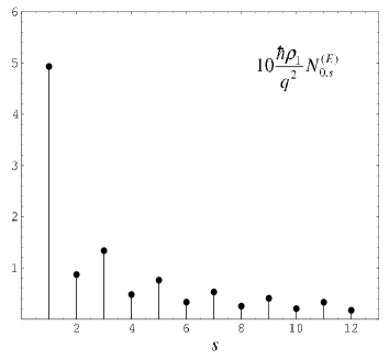
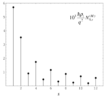
Figure 1: The number of the radiated quanta on the mode $m=0$ as a function of the harmonic number $s$ for the waves of the E- (left panel) and M-type (right panel) (for the values of the parameters see the text).

The values of the parameter $\rho_{1}\lambda_{0,s}^{\mathrm{(F)}}$ for the first eight harmonics are presented in the table. The corresponding frequencies are related to this parameter by the formula $\omega_{0,s}^{\mathrm{(F)}}=v_{\parallel}\lambda_{0,s}^{\mathrm{(E)}}/\sqrt{\beta_{0\parallel}^{2}-1}$.

$s$	1	2	3	4	5	6	7	8
$\rho_{1}\lambda_{0,s}^{\mathrm{(E)}}$	2.728	5.931	9.102	12.262	15.415	18.565	21.713	24.860
$\rho_{1}\lambda_{0,s}^{\mathrm{(M)}}$	2.507	5.653	8.801	11.947	15.092	18.236	21.380	24.523

4 Conclusion

We have considered the electromagnetic field generated by a charged particle moving along a helical orbit inside a dielectric cylinder immersed into a homogeneous medium. The fields and the spectral-angular distribution of the radiation intensity in the exterior medium have been investigated in our previous paper [14]. In particular, the conditions were specified under which strong narrow peaks appear in the angular distribution for the number of radiated quanta. In the present paper we study the fields inside the cylinder. By using the corresponding formulae for the components of the Green function, we have derived expressions for the electromagnetic potentials and fields. These expressions are presented in the form of sums of two terms. The first ones correspond to the fields generated by the charge in a homogeneous medium with the same dielectric permittivity as that for the material of the cylinder. The second terms are induced by the difference of the dielectric permittivities for the exterior and interior media, and are given by formulae (15), (20), (22). We have extracted the parts of the fields which are responsible for the radiation. For the radiation propagating inside the cylinder the projection of the wave vector on the cylinder axis takes discrete set of values which are solutions to the eigenmode equation (30). The expressions for the electromagnetic fields corresponding to the radiation propagating inside the cylinder are derived. As an application we have considered the radiation intensity on the mode $m=0$. In this case the radiation field is separated into purely TE and TM modes and we have found the intensities for both types of these modes determined by formulae (48). These formulae presents the intensities as sums over the modes of the dielectric waveguide. However, as the corresponding eigenmodes are not explicitly known, this form is not convenient for the numerical evaluation of the radiation intensity. In Appendix, by using the generalized Abel-Plana formula, we derive a summation formula for the series over the normal modes of the dielectric cylinder which allows to extract from the radiation intensity the parts corresponding to the radiation in a homogeneous medium and to present the inhomogeneity-induced part in terms of exponentially converging integrals. Unlike to the parts corresponding to the homogeneous medium, the terms induced by the presence of the cylinder are finite also in the case when the dispersion is absent. We have specified the condition under which the influence of dispersion on the inhomogeneity-induced effects can be neglected.

Appendix A Summation formula over the eigenmodes

In this section we derive a summation formula for the series over zeros of the function

$$C_{\alpha}(\eta,z)=V_{\alpha}\{J_{0}(z),K_{0}(\eta z)\},$$ (51)

where and in what follows for given functions $F(z)$ and $G(z)$ we use the notation

$$V\{F(z),G(\eta z)\}=F(z)G^{\prime}(\eta z)+\alpha\eta F^{\prime}(z)G(\eta z),$$ (52)

with $\alpha\geqslant 1$ and $\eta$ being real constants. For this we will use the generalized Abel-Plana formula from [17] (for applications of the generalized Abel-Plana formula in quantum field theory with boundaries see [18]). In this formula we substitute

$$g(z)=if(z)\frac{V_{\alpha}\left\{Y_{0}(z),K_{0}(\eta z)\right\}}{C_{\alpha}(\eta,z)}.$$ (53)

For the combinations of the functions entering in the generalized Abel-Plana formula one has

$$f(z)-(-1)^{k}g(z)=f(z)\frac{V_{\alpha}\{H_{0}^{(k)}(z),K_{0}(\eta z)\}}{C_{\alpha}(\eta,z)},$$ (54)

where $H_{\nu}^{(k)}(z)$, $k=1,2$, are the Hankel functions. Let us denote positive zeros of the function $C_{\alpha}(\eta,z)$ by $k_{s}$, $s=1,2,\ldots$, assuming that these zeros are arranged in the ascending order. Note that, for $z\gg 1$ we have $C_{\alpha}(\eta,z)\approx K_{0}^{\prime}(\eta z)-\alpha\eta zK_{0}(\eta z)/2<0$ and, hence, $k_{s}\gtrsim 1$. By using the asymptotic formulae for the cylindrical functions for large values of the argument, it can be seen that for large values $s$ one has $k_{s}\approx-\arctan(1/\alpha\eta)+\pi/4+\pi s$. For the derivative of the function $C_{\alpha}(\eta,z)$ at the zeros $k_{s}$ one obtains

$$C_{\alpha}^{\prime}(\eta,z)=-\eta\frac{K_{0}(\eta z)}{J_{0}(z)}\left[\alpha(1+\alpha\eta^{2})J_{0}^{\prime 2}(z)+(\alpha-1)J_{0}^{2}(z)\right],\;z=k_{s}.$$ (55)

In particular, it follows from here that the zeros are simple. Assuming that the function $f(z)$ is analytic in the right half-plane, for the residue term in the generalized Abel-Plana formula one finds

$$\underset{z=k_{s}}{\mathrm{Res}}g(z)=-\frac{i}{\pi}T_{\alpha}(k_{s})f(k_{s}),$$ (56)

where we have introduced the notation

$$T_{\alpha}(z)=\frac{2\alpha/z}{\alpha(1+\alpha\eta^{2})J_{0}^{\prime 2}(z)+(\alpha-1)J_{0}^{2}(z)}.$$ (57)

Substituting the expressions for the separate terms into the generalized Abel-Plana formula we obtain the following result

$$\lim_{x_{0}\rightarrow\infty}\left[\sum_{s=1}^{s_{0}}T_{\alpha}(k_{s})f(k_{s})-\int_{0}^{x_{0}}dx\,f(x)\right] = -\frac{1}{\pi}\int_{0}^{\infty}dx\,\left[f(ix)\frac{V_{\alpha}\{K_{0}(x),H_{0}^{(2)}(\eta x)\}}{V_{\alpha}\{I_{0}(x),H_{0}^{(2)}(\eta x)\}}\right.$$ (58)

$$\left.+f(-ix)\frac{V_{\alpha}\{K_{0}(x),H_{0}^{(1)}(\eta x)\}}{V_{\alpha}\{I_{0}(x),H_{0}^{(1)}(\eta x)\}}\right],$$

where $s_{0}$ is defined by the relation $k_{s_{0}}<x_{0}<k_{s_{0}+1}$. This formula is valid for functions $f(z)$ obeying the condition

$$|f(z)|<\epsilon(x)e^{c|y|},\;z=x+iy,\;|z|\rightarrow\infty,$$ (59)

where $c<2$ and $\epsilon(x)\rightarrow 0$ for $x\rightarrow\infty$. Formula (58) is further simplified for functions satisfying the additional condition $f(-ix)=-f(ix)$:

$$\lim_{x_{0}\rightarrow\infty}\left[\sum_{s=1}^{s_{0}}T_{\alpha}(k_{s})f(k_{s})-\int_{0}^{x_{0}}dx\,f(x)\right]=-\frac{4i\alpha}{\pi^{2}}\int_{0}^{\infty}dx\,\frac{f(ix)}{x^{2}g_{\alpha}(\eta,x)},$$ (60)

where

$$g_{\alpha}(\eta,x) = I_{0}^{2}(x)\left[J_{1}^{2}(\eta x)+Y_{1}^{2}(\eta x)\right]+\alpha^{2}\eta^{2}I_{1}^{2}(x)\left[J_{0}^{2}(\eta x)+Y_{0}^{2}(\eta x)\right]$$ (61)

$$-2\alpha\eta I_{0}(x)I_{1}(x)\left[J_{0}(\eta x)J_{1}(\eta x)+Y_{0}(\eta x)Y_{1}(\eta x)\right].$$

Note that we have denoted $g_{\alpha}(\eta,x)=|V\{I_{0}(z),H_{0}^{(1)}(\eta z)\}|^{2}$ and this function is always nonnegative.

References

• [1] Synchrotron Radiation Theory and Its Development, edited by V.A. Bordovitsyn (World Scientific, Singapore, 1999).
• [2] A. Hofman, The Physics of Sinchrotron Radiation (Cambridge University Press, Cambridge, 2004).
• [3] L.Sh. Grigoryan, A.S. Kotanjyan, and A.A. Saharian, Izv. Akad. Nauk Arm. SSR Fiz. 30, 239 (1995) [Sov. J. Contemp. Phys. 30, 1 (1995)].
• [4] S.R. Arzumanian, L.Sh. Grigoryan, Kh.V. Kotanjyan, and A.A. Saharian, Izv. Akad. Nauk Arm. SSR Fiz. 30, 106 (1995) [Sov. J. Contemp. Phys. 30, 12 (1995)].
• [5] L.Sh. Grigoryan, H.F. Khachatryan, and S.R. Arzumanyan, Izv. Akad. Nauk Arm. SSR Fiz. 33, 267 (1998) [Sov. J. Contemp. Phys. 33, 1 (1998)], cond-mat/0001322.
• [6] A.S. Kotanjyan, H.F. Khachatryan, A.V. Petrosyan, and A.A. Saharian, Izv. Akad. Nauk Arm. SSR Fiz. 35, 115 (2000) [Sov. J. Contemp. Phys. 35, 1 (2000)].
• [7] A.S. Kotanjyan and A.A. Saharian, Izv. Akad. Nauk Arm. SSR Fiz. 36, 310 (2001) [Sov. J. Contemp. Phys. 36, 7 (2001)].
• [8] L.Sh. Grigoryan, H.F. Khachatryan, and S.R. Arzumanyan, Izv. Akad. Nauk Arm. SSR Fiz. 37, 327 (2002) [Sov. J. Contemp. Phys. 37, 1 (2002)].
• [9] A.S. Kotanjyan and A.A. Saharian, Mod. Phys. Lett. A 17, 1323 (2002).
• [10] A.S. Kotanjyan, Nucl. Instrum. Methods B201, 3 (2003).
• [11] L.Sh. Grigoryan, H.F. Khachatryan, S.R. Arzumanyan, and M.L. Grigoryan, Nucl. Instrum. Methods B, in press; hep-th/0512106.
• [12] A.A. Saharian and A.S. Kotanjyan, Izv. Akad. Nauk Arm. SSR Fiz. 38, 288 (2003) [Sov. J. Contemp. Phys. 38, 5 (2003)].
• [13] A.A. Saharian and A.S. Kotanjyan, Nucl. Instrum. Methods B226, 351 (2004).
• [14] A.A. Saharian and A.S. Kotanjyan, J. Phys. A 38, 4275 (2005).
• [15] L.A. Gevorgian and P.M. Poghosian, Izv. Akad. Nauk Arm. SSR Fiz. 19, 239 (1984).
• [16] J.D. Jackson, Classical Electrodynamics (John Wiley & Sons, 1998).
• [17] A.A. Saharian, ”The generalized Abel-Plana formula. Applicatons to Bessel functions and Casimir effect,” Report No. IC/2000/14, hep-th/0002239.
• [18] A.A. Saharian, ”Generalized Abel-Plana formula as a renormalization tool in quantum field theory with boundaries,” hep-th/0609093.