hep–th/0609079

On the velocity and chemical-potential dependence of the heavy-quark interaction in ${\cal N}=4$ SYM plasmas

Spyros D. Avramis^1,2,x Konstadinos Sfetsos²x andx Dimitrios Zoakos^2,∗

${}^{1}\!$ Department of Physics, National Technical University of Athens,

15773, Athens, Greece

${}^{2}\!$ Department of Engineering Sciences, University of Patras,

26110 Patras, Greece

avramis@mail.cern.ch,   sfetsos@upatras.gr,   dzoakos@upatras.gr

Abstract

We consider the interaction of a heavy quark-antiquark pair moving in ${\cal N}=4$ SYM plasma in the presence of non-vanishing chemical potentials. Of particular importance is the maximal length beyond which the interaction is practically turned off. We propose a simple phenomenological law that takes into account the velocity dependence of this screening length beyond the leading order and in addition its dependence on the R-charge. Our proposal is based on studies using rotating D3-branes.

 ^∗​ Currently serving in the Hellenic Armed Forces.

1 Introduction and summary

Since the early days of the AdS/CFT correspondence [2], there has been considerable interest in applying string-theoretical techniques for the computation of the interaction potential of an external heavy $q\bar{q}$ pair, as given by the expectation value of a Wilson loop, first demonstrated in [3] for the conformal case. In extensions of this work to non-conformal cases, it was often found that there exists a maximal length beyond which the interaction is practically turned off, the archetypal example being finite-temperature ${\cal N}=4$ SYM theory, described by non-extremal D3-branes [4]. This phenomenon of complete screening persists [5] in the ${\cal N}=4$ theory with chemical potentials, modelled using rotating D3-brane solutions, as well as in the Coulomb branch of the theory, modelled by continuous distributions of D3-branes, even though in that latter case half of the maximal supersymmetries are preserved. Although such results would be hard to obtain using conventional field theoretical methods, their relevance for real QCD was obscured both by the major qualitative differences between QCD and SYM theories and by the fact that the quark-gluon plasma (QGP) used for the experimental study of thermal QCD was until recently thought to be a weakly-coupled collection of quasiparticles [6].

This situation changed drastically after the realization that the QGP is a state of matter best described as a strongly-coupled liquid, but still exhibiting partial deconfinement of color charges (see e.g. [7] for reviews). These features motivate the study of various quantities of physical interest within the gravity/gauge theory correspondence. The best-studied examples encouraging this line of thought are the calculation of the shear viscosity in ${\cal N}=4$ SYM [8] and the various calculations of the rate of energy loss of partons moving through the plasma [9]-[17], both of which lead to results that are in good qualitative agreement with experiment.

This renewed interest shed light into some, often overlooked, aspects of Wilson-loop calculations of heavy-quark potentials. One such aspect is that, in real experimental situations, neutral $q\bar{q}$ pairs are produced with some velocity relative to the plasma, a fact that affects the interaction potential of the pair. Such considerations apply, for example, to the effect of charmonium suppression, the dissociation of $J/\psi$ mesons due to color screening by the deconfining medium [18, 19], an effect that is expected to be enhanced when the $J/\psi$ has a nonzero velocity with respect to the plasma. Although dynamical processes of this kind would be hard to study using conventional methods, they can be addressed rather easily within the gauge/gravity correspondence. In particular, the non-extremal brane metrics serving as gravity duals of finite-temperature gauge theories are, unlike their extremal counterparts, sensitive to boosts in the directions along the brane where the gauge theory resides. Then, the computation of the potential interaction of a $q\bar{q}$ pair moving with respect to the thermal plasma is simply accomplished by applying the standard AdS/CFT calculation of Wilson loops to such boosted backgrounds. The first examples of finite-temperature computations of this kind were done for a confining non-supersymmetric theory in [21] and for ${\cal N}=4$ SYM at vanishing R-charge in [22, 23] (see also [24, 25] for further works). The results of [22], in particular, suggest a universal law for the behavior of the maximum screening length was suggested, essentially stating that it depends mainly as $(1-v^{2})^{1/4}$ on the pair’s velocity, perfectly valid for ultrahigh velocities. Given the importance of such a law for building up phenomenological models for certain effects occurring in hot plasmas, it is interesting to ask how this law is affected when chemical potentials are turned on and what are the details of the velocity dependence. In this paper, we examine precisely these two issues, within the AdS/CFT correspondence, using rotating D3-brane solutions. In principle, the maximal screening length can be a function of the plasma parameters, namely the temperature and the R-charge density and in addition it depends on the velocity vector of the $q\bar{q}$ pair.

Our studies suggest a law that can be used in phenomenological models, namely that the maximal length has the following form in the rest frame of the $q\bar{q}$ pair

$$q\bar{q}{\rm\ rest\ frame}:\phantom{xxx}L_{\rm max}={\cal F}(v,\xi)\ {G(\xi)\over\pi T}\ {1\over\gamma^{{1/2}}}\left(1+c_{1}{\lambda^{2}\over\gamma}+{c_{2}+c_{3}\lambda^{4}\over\gamma^{2}}\right)\ ,$$ (1.1)

with the definitions

$$\gamma={1\over\sqrt{1-v^{2}}}\ ,\qquad\xi\sim{J\over N^{2}T^{3}}\ .$$ (1.2)

This form is not very sensitive to the orientation of the axis of the pair as compared with its velocity. In particular, the average value of the maximal length over the corresponding angle is, under reasonable assumptions on the angle distribution of the produced $q\bar{q}$ pairs, basically of the same form as well. In the above, $N$ is the number of colors, $T$ is the plasma temperature and $J$ is the R-charge density. Also, $\xi$ is the dimensionless R-charge parameter (the overall numerical value in its definition will be fixed later), while $\lambda=\lambda(\xi)$ is a dimensionless function of $\xi$ ranging between zero and an upper bound of order one. Finally, $c_{i}$, with $i=1,2,3$, are numerical parameters which, although in our models they have precisely determined values, relatively small compared to unity, in more realistic experimental situations they should be fitted to data. The leading term in Eq. (1.1), which dominates in the ultrarelativistic (large-$\gamma$) limit, was already suggested by the computation of [22]. However, we shall see that in our models it makes sense to include the other two terms since they become important for not too extremely relativistic velocities, i.e. for $v\lesssim 0.8$. The function ${\cal F}(v,\xi)$ has a very weak functional dependence and can be practically taken to be constant. The function $G(\xi)$ has a behavior of the form $G(\xi)=1+{\cal O}(\xi^{2})$ for small $\xi$-values, but can otherwise have either weak or strong dependence on the parameter $\xi$, depending on the model. In particular, in cases with $\xi\gg 1$, we have the behavior $G(\xi)\sim\xi^{-1/3}$, signifying that the screening length becomes temperature-independent and its scale is set by the R-charge density $J$. In addition, a dependence proportional to $N^{2/3}$ arises. For experimentally-motivated studies however, one may compare ratios of maximal screening lengths at different velocities so that any strong dependence on the chemical potential cancels out. We note that in [25] it has been shown that the leading velocity dependence of the screening length is of the form $(1-v^{2})^{\nu}$, where the exponent $\nu={1\over 4}$ in ${\cal N}=4$ theories, but is lower than that in certain cases with less supersymmetry. Based on that we may further generalize (1.1) and replace in the exponent of the leading order term the $1/2$ by the parameter $2\nu$. We do not believe that this generalization will affect the form of the correction terms, as they appear essentially from the analyticity properties of integrals below. The same replacement can be done for the analogous formulae below.

In the rest frame of the plasma, we should also take into account the Lorentz contraction of the component of the length along the direction of the motion. In this case the result is sensitive to the actual distribution probability for the angle between the $q\bar{q}$-pair axis and its velocity vector. The most reasonable assumption is that, that this probability is uniform in the plasma rest frame. Then, based on our computations, we suggest the following law

$${\rm Plasma\ rest\ frame}(1):\phantom{xx}L_{\rm max}={\cal F}(v,\xi)\ {G(\xi)\over\pi T}\ {1+a\ln\gamma\over\gamma^{{3/2}}}\left(1+d_{1}{\lambda^{2}\over\gamma}+{d_{2}+d_{3}\lambda^{4}\over\gamma^{2}}\right)\ ,$$ (1.3)

where again we have averaged over the angle formed by the $q\bar{q}$-pair’s axis and its velocity vector. The numerical parameters $a$ and $d_{i}$, $i=1,2,3$ are to be fitted to possible experimental results. Note that, compared to (1.1), we have a suppression factor $1/\gamma$ as as well as the presence of a $\ln\gamma$ term in the overall coefficient. As we will show, these are due to the dominance, in taking the average, of pairs with their axis almost parallel to their velocity vector.

A second possibility, less likely in our opinion, is that the angle distribution be uniform in the pair’s rest frame. In this case, instead of (1.3) we have

$${\rm Plasma\ rest\ frame}(2):\phantom{xx}L_{\rm max}={\cal F}(v,\xi)\ {G(\xi)\over\pi T}\ {1\over\gamma^{{1/2}}}\left(1+d_{1}{\lambda^{2}\over\gamma}+{d_{2}+d_{3}\lambda^{4}+d_{4}\ln\gamma\over\gamma^{2}}\right)\ ,$$ (1.4)

where again we have averaged over the angle. Note that in this case we have no extra suppression in the length compared to (1.1), with the exception of the appearance of $\ln\gamma$ in a subleading term. Hence in this case we have a dominance of angles near $\Theta=\pi/2$, at which the length suffers no Lorentz contraction.

The organization of this paper is as follows. In section 2 we set up the general formalism for computing the interaction potential of moving $q\bar{q}$ pairs in general backgrounds. In section 3 we review the zero R-charge case and in section 4 we compute the maximal screening length for more general situations having non-zero R-charge using rotating D3-brane solutions. Finally, in section 5 we consider issues concerning the screening length in the plasma rest frame versus the quark pair rest frame as well as their average values.

2 Moving $q\bar{q}$ pairs in the ${\cal N}=4$ plasma

In the framework of AdS/CFT, Wilson-loop calculations for a $q\bar{q}$ pair moving with velocity $v$ relative to the plasma can be carried our either in the rest frame of the plasma where one considers a string whose endpoints move with velocity $v$ or, equivalently, in the rest frame of the $q\bar{q}$ pair, where one considers a string with fixed endpoints in a boosted background. In what follows, we will employ the second approach.

To describe the method, we begin with a general ten-dimensional metric of the form

$$ds^{2}=G_{tt}dt^{2}+G_{xx}dx^{2}+G_{yy}dy^{2}+G_{rr}dr^{2}+\cdots\ ,$$ (2.1)

where the metric components do not depend on $t,x$ and $y$ and where the ellipses denote the remaining terms involving all other variables. These could be either cyclic variables similar to $x$ and $y$ or angular variables that can be set to some constant values consistent with their equations of motion. Orienting the axes so that the $q\bar{q}$ pair moves along the negative $x$ direction, and applying a boost in this direction, we obtain the metric

$$d\hat{s}^{2}=\hat{G}_{tt}dt^{2}+\hat{G}_{xx}dx^{2}+2\hat{G}_{tx}dtdx+G_{yy}dy^{2}+G_{rr}dr^{2}+\cdots\ ,$$ (2.2)

where

$$\hat{G}_{tt}=\gamma^{2}(G_{tt}+v^{2}G_{xx})\ ,\qquad\hat{G}_{xx}=\gamma^{2}(v^{2}G_{tt}+G_{xx})\ ,\qquad\hat{G}_{tx}=-\gamma^{2}v(G_{tt}+G_{xx})\ .$$ (2.3)

The separation length and energy of a $q\bar{q}$ pair of arbitrary orientation with respect to the plasma velocity is found by considering a Wilson loop on a rectangular contour $C$ with one side of length $T$ along the $t$ direction and one side of length $L$ along a spatial direction, taken for definiteness to be parallel to the $xy$ plane and tilted at an angle $\Theta$ relative to the $x$ axis, as shown in Fig. 1.

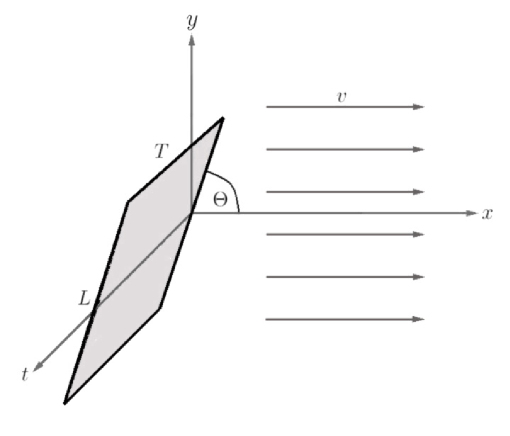
Figure 1: Wilson loop for the energy computation of a $q\bar{q}$ pair in a moving plasma (shaded rectangle).

Then, according to the gauge/gravity correspondence, the interaction potential energy $E$ of the $q\bar{q}$ pair, as measured by the Wilson loop expectation $\langle W(C)\rangle$, is given by [3]

$$e^{-iET}=\langle W(C)\rangle=e^{iS[C]}\ ,$$ (2.4)

where

$$S[C]=-{1\over 2\pi}\int d\tau d\sigma\sqrt{-\det g_{\alpha\beta}}\ ,\qquad g_{\alpha\beta}=\hat{G}_{\mu\nu}\partial_{\alpha}x^{\mu}\partial_{\beta}x^{\nu}\ ,$$ (2.5)

is the Nambu–Goto action for a string propagating in the boosted supergravity background, whose endpoints trace the contour $C$. We note that we will use Minkowski signature throughout the paper. Fixing reparametrization invariance by taking $(\tau,\sigma)=(t,y)$, assuming translational invariance along the $t$ direction and setting all angles to constants (to specific values consistent with the equations of motion), the embedding of the string is described by the functions

$$r=u(y)\ ,\qquad x=x(y)\ ,\qquad{\rm rest}={\rm const.}\ ,$$ (2.6)

and the boundary condition for the string endpoints becomes

$$u\left(\pm{L\over 2}\sin\Theta\right)=\infty\ ,\qquad x\left(\pm{L\over 2}\sin\Theta\right)=\pm{L\over 2}\cos\Theta\ .$$ (2.7)

The Nambu–Goto action is then written in the form

$$S[C]=-{T\over 2\pi}\int dy\sqrt{f_{y}(u)+f_{x}(u)x^{\prime 2}+g(u)u^{\prime 2}}\ ,$$ (2.8)

where the prime denotes a derivative with respect to $y$ and

$$f_{y}(u)=-\gamma^{2}G_{yy}(G_{tt}+v^{2}G_{xx})\ ,\qquad f_{x}(u)=-G_{tt}G_{xx}\ ,$$

$$g(u)=-\gamma^{2}G_{rr}(G_{tt}+v^{2}G_{xx})\ .$$ (2.9)

Since actions of the precise form (2.8) have been encountered in the static Wilson-loop calculations for $x^{\prime}=0$ in [5] (see section 1) and [26] (see section 5, where $x$ played the role of an angular variable), we briefly review the results without entering into the intermediate computational details. Independence of the Lagrangian from $y$ and $x$ leads to two first-order equations expressing the conservation of the “energy” and the momentum $\pi_{x}$ conjugate to $x(y)$. Integrating these equations, one obtains [26]

$$L\sin\Theta = 2\sqrt{1-\pi_{x}^{2}}\ f_{y}^{1/2}(u_{0})\int_{u_{0}}^{\infty}{du\over f_{y}(u)}\sqrt{g(u)\over F(u)}\ ,$$

$$L\cos\Theta = 2\pi_{x}\ f_{x}^{1/2}(u_{0})\int_{u_{0}}^{\infty}{du\over f_{x}(u)}\sqrt{g(u)\over F(u)}\ ,$$ (2.10)

where the integration constant $u_{0}$ is the value where $u(y)$ develops a minimum. Substituting them in the Nambu–Goto action, one finds the $q\bar{q}$ potential energy

$$E={1\over\pi}\int^{\infty}_{u_{0}}du\sqrt{g(u)\over F(u)}-E_{0}\ .$$ (2.11)

where $E_{0}$ is the subtraction term corresponding to the energy of two disconnected worldsheets, to be discussed below. In the above, the function $F(u)$ is defined by

$$F(u)=1-\pi_{x}^{2}{f_{x}(u_{0})\over f_{x}(u)}-(1-\pi_{x}^{2}){f_{y}(u_{0})\over f_{y}(u)}\ .$$ (2.12)

and satisfies $F(u_{0})=0$. The system of Eqs. (2) implicitly determines the parameters $u_{0}$ and $\pi_{x}$ in terms of the separation length $L$ and the angle $\Theta$, the latter clearly only via the combinations $\cos^{2}\Theta$ and $\sin^{2}\Theta$. Substituting the resulting values into (2.11) gives the potential energy for the same parameters. Note that Eqs. (2)-(2.12) are invariant under the symmetry operation $\Theta\to{\pi\over 2}-\Theta$ followed by the exchange of the $x$ and $y$ indices and the renaming $\pi_{x}^{2}\to 1-\pi_{x}^{2}$.

To avoid unnecessary complications, we will restrict to the cases where the spatial side of the Wilson loop is either perpendicular ($\Theta={\pi\over 2}$) or parallel ($\Theta=0$) to the plasma velocity and only discuss the general case in section 5. In the first case, we have $\pi_{x}=0$ and so the length and energy read [5]

$$L=2f_{y}^{1/2}(u_{0})\int_{u_{0}}^{\infty}du\sqrt{g(u)\over f_{y}(u)[f_{y}(u)-f_{y}(u_{0})]}\ ,$$ (2.13)

and

$$E={1\over\pi}\int^{\infty}_{u_{0}}du\sqrt{g(u)f_{y}(u)\over f_{y}(u)-f_{y}(u_{0})}-E_{0}\ ,$$ (2.14)

while in the second case we have $\pi_{x}=1$ and the length and energy are given by the above formulas with the replacement $f_{y}\to f_{x}$.

At this point, some clarifying comments are in order. A first issue is how much the string may stretch into the radial direction, i.e. which is the minimum allowed value for the turning point $u_{0}$. To examine this issue, we note that in the geometries under consideration there appear several special values of the radius, namely (i) the horizon radius $u_{H}$ where $g(u)$ blows up, (ii) the radius $u_{e}$ where $f_{x}(u)$ becomes zero, which in our examples, depending on the angle, coincides with the maximum or minimum values of the ergosphere (which, in the absence of rotation, coincides with $u_{H}$) and (iii) the velocity-dependent radius $u_{v}$ where $g(u)$ and $f_{y}(u)$ become zero (which, in the zero-velocity limit, coincides with $u_{H}$). In our examples, these radii always satisfy $u_{H}\leqslant u_{e}\leqslant u_{v}$. While it is quite obvious that taking $u_{0}\geq u_{v}$ is always consistent, some care is needed in order to examine whether we can take $u_{0}<u_{v}$. To this end, we distinguish between two cases. When $\Theta\neq 0$, the first of Eqs. (2) is always relevant and the factor $\sqrt{f_{y}(u_{0})}$ in that equation becomes imaginary for $u_{0}<u_{v}$, therefore excluding that possibility. On the other hand, when $\Theta=0$, the first of Eqs. (2) becomes irrelevant and the behavior of the string is solely determined by the function $x(u)$ with $x^{\prime}(u)\sim\sqrt{f_{x}(u_{0})}{\sqrt{g(u)}\over f_{x}(u)\sqrt{F(u)}}$. If we take $u_{0}<u_{v}$ then the string will first reach the radius $u_{v}$ where $x^{\prime}(u)$ becomes zero so that the string develops a cusp and cannot be further extended towards $u_{0}$. If one wishes to include such configurations, one must thus cut off the region $u_{0}\leqslant u<u_{v}$ by replacing the lower limit of the integrations from $u_{0}$ to $u_{v}$ for all $u_{0}<u_{v}$. However, since (i) string configurations with cusps raise questions about the validity of the Nambu–Goto approach since the string curvature diverges there, (ii) the maximal value of $L(u_{0})$, which is the main quantity of interest in this paper, corresponds to a value $u^{\rm c}_{0}$ of $u_{0}$ that is always larger than $u_{v}$, and (iii) the region $u_{0}<u^{\rm c}_{0}$ where cusps may appear corresponds to a branch of the solution (with the same prescribed boundary conditions (2.7)) which is energetically unfavorable and thus presumably unstable, we will altogether ignore the presence of cusps as they are irrelevant for our screening problem.

Another issue refers to the choice of subtraction term $E_{0}$ in (2.11). In the zero-velocity case, the subtraction term is unique and represents two straight strings stretching from infinity to the horizon. In the case of nonzero velocity, however, the above configuration is no longer a solution to the equations of motionand one must find an appropriate subtraction term that (i) removes the divergence, (ii) is consistent with the equations of motion, (iii) is independent of the separation length and (iv) reduces in the zero-velocity limit to two straight strings stretching to the horizon. These criteria are satisfied by any configuration of two disconnected strings interpolating between the drag configuration of [9] (and its generalizations [10] for the case of rotating branes), which represents a curved string stretching up to the horizon $u_{H}$ and a configuration of one straight string stretching up to the radius $u_{v}\geqslant u_{H}$. Note that in order for the strings to end at a radius larger than $u_{H}$, one needs to assume the presence of a second flavor brane at that radius, in which case each string should be regarded as dual to a meson composed out of a heavy and a light quark (like a bottom and an up or a down quark). Be that as it may, there seems to exist an infinite family of subtraction terms [27] consistent with the above requirements. The maximum subtraction energy [23] corresponds to the drag configuration and is given by

$$E_{0}={1\over\pi}\int_{u_{H}}^{\infty}du\ ,$$ (2.15)

while the minimum subtraction energy corresponds to the straight-string configuration and reads

$$E_{0}={1\over\pi}\int_{u_{v}}^{\infty}du\sqrt{g(u)}\ .$$ (2.16)

Among the possible subtraction terms, the one corresponding to the drag configuration seems to be the most sensible one, as it is the only solution available in the absence of an extra flavor brane.

3 Screening in the zero–R-charge case

In order to establish our notation and present some extra details, we first review the zero–R-charge case, examined in [22] and also in [23]. In this case, the background geometry has metric

$$ds^{2}={r^{2}\over R^{2}}\left[-\left(1-{\mu^{4}\over r^{4}}\right)dt^{2}+dx^{2}+dy^{2}+dz^{2}\right]+{R^{2}r^{2}\over r^{4}-\mu^{4}}\ dr^{2}+R^{2}d\Omega_{5}^{2}\ ,$$ (3.1)

where the horizon is located at $r=\mu$ and the Hawking temperature is $T={\mu\over\pi R^{2}}$. Then we have for the various functions

$$f_{y}(u)={1\over R^{4}}(u^{4}-\gamma^{2}\mu^{4})\ ,\qquad f_{x}(u)={1\over R^{4}}(u^{4}-\mu^{4})\ ,\qquad g(u)={u^{4}-\gamma^{2}\mu^{4}\over u^{4}-\mu^{4}}\ .$$ (3.2)

3.1 Motion perpendicular to the $q\bar{q}$-pair axis

Let us first consider the $\Theta={\pi\over 2}$ case corresponding to plasma velocities perpendicular to the axis of the $q\bar{q}$ pair. Substituting $f_{y}(u)$ and $g(u)$ from (3.2) into Eqs. (2.13) and (2.14), introducing the dimensionless length and energy parameters

$$\ell=\pi TL\ ,\qquad\varepsilon={1\over R^{2}T}E\ ,$$ (3.3)

and trading $u$ and $u_{0}$ for the dimensionless variables $y={u\over\mu}$ and $y_{0}={u_{0}\over\mu}\geqslant\sqrt{\gamma}$, we obtain for the length

$$\ell(v,y_{0}) = 2\sqrt{y_{0}^{4}-\gamma^{2}}\int_{y_{0}}^{\infty}{dy\over\sqrt{(y^{4}-1)(y^{4}-y_{0}^{4})}}$$ (3.4)

$$= {2\sqrt{2}\pi^{3/2}\over\Gamma(1/4)^{2}}\ {\sqrt{y_{0}^{4}-\gamma^{2}}\over y_{0}^{3}}\ {}_{2}F\!_{1}\left({1\over 2},{3\over 4},{5\over 4},{1\over y_{0}^{4}}\right)\ ,$$

where ${}_{2}F\!_{1}(a,b,c,x)$ denotes the standard hypergeometric function. For the energy, use of the maximum subtraction (2.15) leads to the result

$$\varepsilon(v,y_{0}) = \int_{y_{0}}^{\infty}dy\left[{y^{4}-\gamma^{2}\over\sqrt{(y^{4}-1)(y^{4}-y_{0}^{4})}}-1\right]-(y_{0}-1)$$ (3.5)

$$= -{\sqrt{2}\pi^{3/2}\over\Gamma(1/4)^{2}}\left[y_{0}\ {}_{2}F\!_{1}\left(-{1\over 4},{1\over 2},{1\over 4},{1\over y_{0}^{4}}\right)+{\gamma^{2}\over y_{0}^{3}}\ {}_{2}F\!_{1}\left({1\over 2},{3\over 4},{5\over 4},{1\over y_{0}^{4}}\right)\right]+1\ ,$$

while use of the minimum subtraction (2.16) yields

$$\varepsilon(v,y_{0}) = \int_{y_{0}}^{\infty}dy\left[{y^{4}-\gamma^{2}\over\sqrt{(y^{4}-1)(y^{4}-y_{0}^{4})}}-\sqrt{{y^{4}-\gamma^{2}\over y^{4}-1}}\right]-\int_{\sqrt{\gamma}}^{y_{0}}dy\sqrt{{y^{4}-\gamma^{2}\over y^{4}-1}}$$

$$= -{\sqrt{2}\pi^{3/2}\over\Gamma(1/4)^{2}}\biggl{[}y_{0}\ {}_{2}F\!_{1}\left(-{1\over 4},{1\over 2},{1\over 4},{1\over y_{0}^{4}}\right)+{\gamma^{2}\over y_{0}^{3}}\ {}_{2}F\!_{1}\left({1\over 2},{3\over 4},{5\over 4},{1\over y_{0}^{4}}\right)$$

$$\qquad\qquad\quad-2\sqrt{\gamma}\ {}_{2}F\!_{1}\left({1\over 2},-{1\over 4},{5\over 4},{1\over\gamma^{2}}\right)\biggr{]}\ ,$$

Note that, according to the discussion of section 2, no cusps occur and that the two expressions above differ only by the last term which is velocity dependent, but totally independent of the parameter $u_{0}$. As a result the two expressions differ by an $\ell$-independent term and the force between the quarks, given by minus the derivative of the energy with respect to the separation length, is the same no matter which expression we use. In the static limit in which $\gamma=1$, using properties of the hypergeometric functions, the expressions (3.5) and (3.1) are found to coincide. Also for $\ell\to 0$, both go to the conformal result of [3].

Fig. 2(a) shows the dimensionless energy $\varepsilon$ as a function of the dimensionless separation length $\ell$ for various values of the velocity $v$. We see that $\varepsilon$ is a double-valued function of $\ell$ whose upper branch corresponds to a presumably metastable, at best, configuration and is to be discarded. As in the static case with $v=0$ [4], there is a maximal length $\ell_{\rm max}(v)$ beyond which there is complete screening of the potential since the only allowed configuration is the zero-energy configuration of two disconnected worldsheets. Its numerical value for $v=0$ is $\ell_{\rm max}(0)=0.869$ was given in [5, 22]. For ultrahigh velocities it goes to zero as $\ell_{\rm max}(v\to 1)=0.743\gamma^{-1/2}$ as first noted in [22]. There are various ways to see that. In particular, assuming that $y_{0}\gg 1$, from (3.4) and the fact that the hypergeometric function becomes unity at the origin, we see that $\ell\simeq{2\sqrt{2}\pi^{3/2}\over\Gamma(1/4)^{2}}{\sqrt{y_{0}^{4}-\gamma^{2}}\over y_{0}^{3}}$. Maximization of this with respect to $y_{0}$ gives $y_{0}^{2}=\sqrt{3}\gamma$, which upon substitution gives $\ell_{\rm max}(v\to 1)={4\pi^{3/2}\over 3^{3/4}\Gamma(1/4)^{2}}\gamma^{-1/2}\simeq 0.743\gamma^{-1/2}$, as stated above.

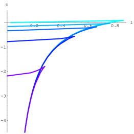
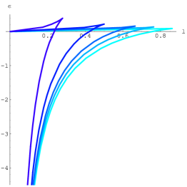
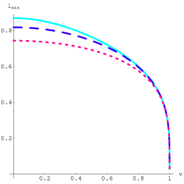
(a)	(b)	(c)

Figure 2: (a,b) Potential energy $\varepsilon$ plotted as a function of the separation $\ell$ for the values $v=0$, $0.5$, $0.7$, $0.9$ and $0.99$ (right to left) using the maximum and minimum subtraction prescriptions respectively. (c) Plots of various approximations to $\ell_{\rm max}(v)$, namely the result of numerical computation (solid), the approximation (1.1) (dashed) and its leading-order form (dotted).

Besides the maximal length, there also exists a value $\ell_{\rm s}(v)$ of the length [22, 23] (its value for $v=0$ is $\ell_{\rm s}(0)=0.754$ [5]) after which the lower branch of $\varepsilon$ takes positive values. The region beyond this point is also to be discarded, since the free configuration becomes energetically favored there, and hence this length could be also used as a definition of the screening length. Using the regularization (3.5) for the energy there is a velocity $v_{c}\simeq 0.447$ for which the maximum length and $\ell_{\rm s}$ coincide [23] and after which there is no distinction between them. Then, as shown in Fig. 2(a), for small velocities the length $\ell_{\rm s}(v)$ differs from the maximal one by about ten percent and, as the velocity is increased, the difference becomes smaller and vanishes for the above value of the velocity $v_{c}$. Since $\ell_{\rm s}$ practically coincides with $\ell_{\max}$ for $v\gtrsim 0.35$, and since its study necessitates examining both $\varepsilon$ and $\ell$ thus requiring more involved numerics, in this paper we will define the screening length as the maximal length allowed.

The above results for $\ell_{\rm max}(v)$ served as a motivation for the authors of [22] to suggest that the velocity dependence of the maximal length is given by the empirical formula

$$\ell_{\rm max}(v)={\cal F}(v)(1-v^{2})^{1/4}\ ,$$ (3.7)

where ${\cal F}(v)$ is a function with relatively weak dependence on $v$, with ${\cal F}(0)=0.869$ and ${\cal F}(1)=0.743$. With an analysis that we will perform in a more general setting in the next section, we will find an improved version of (3.7)

$$\ell_{\rm max}(v)={\cal F}(v)(1-v^{2})^{1/4}\left[1+c_{2}(1-v^{2})^{1/2}\right]\ ,$$ (3.8)

which is of the form (1.1). For our model the numerical coefficient is computed in more general situations below and takes the value $c_{2}=0.100$. In that case ${\cal F}(v)$ is indeed a practically flat function of $v$ since ${\cal F}(0)=0.790$ and ${\cal F}(1)=0.743$. Plots of $\ell_{\rm max}(v)$ in the various approximations considered are shown in Fig. 2(c).

3.2 Motion parallel to the $q\bar{q}$-pair axis

Let us consider next the $\Theta=0$ case, corresponding to plasma velocities along the axis of the $q\bar{q}$ pair. Substituting $f_{x}(u)$ and $g(u)$ in the corresponding equations and employing the same rescalings as before, we find for the length

$$\ell(v,y_{0}) = 2\sqrt{y_{0}^{4}-1}\int_{y_{0}}^{\infty}{dy\over y^{4}-1}\sqrt{y^{4}-\gamma^{2}\over y^{4}-y_{0}^{4}}\ ,$$ (3.9)

$$= {2\sqrt{2}\pi^{3/2}\over\Gamma(1/4)^{2}}\ {\sqrt{y_{0}^{4}-1}\over y_{0}^{3}}\ F\!_{1}\left({3\over 4},-{1\over 2},1,{5\over 4},{\gamma^{2}\over y_{0}^{4}},{1\over y_{0}^{4}}\right)\ ,$$

where $F\!_{1}(a,b_{1},b_{2},c,x,y)$ is the Appell hypergeometric function. For the energy, use of the maximum subtraction (2.15) and the minimum subtraction (2.16) leads to

$$\varepsilon(v,y_{0}) = \int_{y_{0}}^{\infty}dy\left(\sqrt{{y^{4}-\gamma^{2}\over y^{4}-y_{0}^{4}}}-1\right)-(y_{0}-1)\ ,$$ (3.10)

$$= -{\sqrt{2}\pi^{3/2}\over\Gamma(1/4)^{2}}y_{0}\ {}_{2}F\!_{1}\left(-{1\over 2},-{1\over 4},{1\over 4},{\gamma^{2}\over y_{0}^{4}}\right)+1\ .$$

and

$$\varepsilon(v,y_{0}) = \int_{y_{0}}^{\infty}dy\left(\sqrt{y^{4}-\gamma^{2}\over y^{4}-y_{0}^{4}}-\sqrt{{y^{4}-\gamma^{2}\over y^{4}-1}}\right)-\int_{\sqrt{\gamma}}^{y_{0}}dy\sqrt{{y^{4}-\gamma^{2}\over y^{4}-1}}\ ,$$ (3.11)

$$= -{\sqrt{2}\pi^{3/2}\over\Gamma(1/4)^{2}}\left[y_{0}\ {}_{2}F\!_{1}\left(-{1\over 2},-{1\over 4},{1\over 4},{\gamma^{2}\over y_{0}^{4}}\right)-2\sqrt{\gamma}\ {}_{2}F\!_{1}\left({1\over 2},-{1\over 4},{5\over 4},{1\over\gamma^{2}}\right)\right]\ .$$

respectively. Note that, according to the discussion of section 2, one may take $y_{0}<y_{v}=\sqrt{\gamma}$ in which case there may occur cusps. However, the branch where cusps occur is irrelevant for our problem. This subtlety aside, the qualitative behavior discussed in the previous subsection remains virtually unchanged, with only small deviations from the $\Theta={\pi\over 2}$ case. For instance, the numerical coefficient for the $v\to 1$ behavior changes to $0.837$ but nevertheless the velocity dependence remains of the same form. For this reason, in the rest of this paper we will consider in detail only the $\Theta={\pi\over 2}$ case.

4 Screening in the case of nonzero R-charges

In light of the above results, a natural question arising is whether the $(1-v^{2})^{1/4}$ velocity scaling law is universal in more generalized settings, one of which is the ${\cal N}=4$ theory with non-vanishing R-charges. In what follows, we will briefly review the relevant supergravity backgrounds and then we will address the questions (i) whether this velocity dependence persists in the presence of R-charges and (ii) what is the nature of the dependence of the maximal length on the R-charge density.

4.1 Non-extremal rotating branes

According to AdS/CFT, the gravity duals to ${\cal N}=4$, $SU(N)$ SYM theory at finite temperature and R-charge are given by non-extremal rotating D3-brane solutions found in [28, 29]. In the conventions of [30] which we here follow, the field-theory limit of these solutions is characterized by the non-extremality parameter $\mu$ and the angular momentum parameters $a_{i}$, $i=1,2,3$, which are related to three R-charges (or chemical potentials) in the gauge theory. Below we review two special cases of these solutions, corresponding to two equal nonzero angular momenta and one nonzero angular momentum, for which we state the relations between the supergravity and gauge-theory parameters as well as the restrictions on the physical ranges of these parameters as dictated by thermodynamic stability [31]. For more details on the calculations, the reader is referred to [15].

4.1.1 Two equal nonzero angular momenta

We first examine the case of two equal nonzero angular momenta, which we can take as $a_{2}=a_{3}=r_{0}$. The metric is given by

$$ds^{2}=H^{-1/2}\left[-\left(1-{\mu^{4}H\over R^{4}}\right)dt^{2}+dx^{2}+dy^{2}+dz^{2}\right]+H^{1/2}{r^{4}(r^{2}-r_{0}^{2}\cos^{2}\theta)\over(r^{4}-\mu^{4})(r^{2}-r_{0}^{2})}\ dr^{2}$$

$$+H^{1/2}\Big{[}(r^{2}-r_{0}^{2}\cos^{2}\theta)d\theta^{2}+r^{2}\cos^{2}\theta d\Omega_{3}^{2}+(r^{2}-r_{0}^{2})\sin^{2}\theta d\phi_{1}^{2}$$ (4.1)

$$-\ 2{\mu^{2}r_{0}\over R^{2}}\ dt\cos^{2}\theta(\sin^{2}\psi d\phi_{2}+\cos^{2}\psi d\phi_{3})\Big{]}\ ,$$

where

$$H={R^{4}\over r^{2}(r^{2}-r_{0}^{2}\cos^{2}\theta)}\$$ (4.2)

and $d\Omega^{2}_{3}=d\psi^{2}+\sin^{2}\psi d\phi_{2}^{2}+\cos^{2}\psi d\phi_{3}^{2}$ is the $S^{3}$ line element. The horizon is located at

$$r_{H}=\mu\ .$$ (4.3)

On the gravity side, the above solution is characterized by the two parameters $\mu$ and $r_{0}$. On the dual gauge-theory side, it is most natural to use the Hawking temperature $T$ and the angular momentum density $J$, which correspond to the temperature and R-charge density of the gauge theory i.e. to the canonical-ensemble thermodynamic variables. On both sides, it is convenient to trade $r_{0}$ and $J$ for the dimensionless parameters

$$\lambda={r_{0}\over\mu}\ ,\qquad\xi={6\sqrt{3}J\over\pi N^{2}T^{3}}\ .$$ (4.4)

The two sets of parameters $(\mu,\lambda)$ and $(T,\xi)$ are related by

$$\mu=\pi R^{2}T\sqrt{1+Q^{2}}\ ,\qquad\lambda={Q\over\sqrt{1+Q^{2}}}\ ,$$ (4.5)

where $F(\xi)$ is the function

$$Q(\xi)={(\xi+\sqrt{1+\xi^{2}})^{1/3}-(\xi+\sqrt{1+\xi^{2}})^{-1/3}\over\sqrt{3}}\ .$$ (4.6)

Substituting this into (4.5) we obtain the explicit expression for $\lambda=\lambda(\xi)$. The constraints imposed by thermodynamic stability on the parameters $\lambda$, $\xi$ and $Q$ as follows

$$0\leqslant\lambda\leqslant 1\ ,\qquad 0\leqslant\xi<\infty\ ,\qquad 0\leqslant Q<\infty\ .$$ (4.7)

4.1.2 One nonzero angular momentum

We next examine the case of only one nonzero angular momentum, which we can take as $a_{1}=r_{0}$. The metric is given by

$$ds^{2}=H^{-1/2}\left[-\left(1-{\mu^{4}H\over R^{4}}\right)dt^{2}+dx^{2}+dy^{2}+dz^{2}\right]+H^{1/2}{r^{2}(r^{2}+r_{0}^{2}\cos^{2}\theta)\over r^{4}+r_{0}^{2}r^{2}-\mu^{4}}\ dr^{2}$$

$$+H^{1/2}\Big{[}(r^{2}+r_{0}^{2}\cos^{2}\theta)d\theta^{2}+r^{2}\cos^{2}\theta d\Omega_{3}^{2}+(r^{2}+r_{0}^{2})\sin^{2}\theta d\phi_{1}^{2}$$ (4.8)

$$-\ 2{\mu^{2}r_{0}\over R^{2}}\sin^{2}\theta dtd\phi_{1}\Big{]}\ ,$$

where

$$H={R^{4}\over r^{2}(r^{2}+r_{0}^{2}\cos^{2}\theta)}\$$ (4.9)

and the $S^{3}$ line element is as before. The horizon is located at $r=r_{H}$ with

$$r_{H}^{2}={1\over 2}\left(-r_{0}^{2}+\sqrt{r_{0}^{4}+4\mu^{4}}\right)\ .$$ (4.10)

As before, the solution is characterized by $\mu$ and $r_{0}$ on the gravity side and by $T$ and $J$ on the dual gauge-theory side. Introducing again dimensionless variables according to

$$\lambda={r_{0}\over\mu}\ ,\qquad\xi={2\sqrt{2}J\over\pi N^{2}T^{3}}\ ,$$ (4.11)

we find that the two sets of parameters are related by

$$\mu=\pi R^{2}TQ^{3/4}(2-Q)^{1/4}\ ,\qquad\lambda={\sqrt{2}(Q-1)^{1/2}\over Q^{1/4}(2-Q)^{1/4}}\ ,$$ (4.12)

where $Q(\xi)$ is the lower branch of the solution to the equation $Q^{4}(Q-1)(Q-2)+\xi^{2}=0$, which admits a perturbative expansion, near $\xi=0$, as $Q=1+{\cal O}(\xi^{2})$. Again, one may substitute this into (4.12) to obtain a perturbative expansion for $\lambda=\lambda(\xi)$. Finally, thermodynamic stability constrains $\lambda$, $\xi$ and $Q$ as follows

$$0\leqslant\lambda\leqslant\lambda_{0}\simeq 1.46\ ,\qquad 0\leqslant\xi\leqslant\xi_{\rm max}\simeq 1.33\ ,\qquad 1\leqslant Q\leqslant Q_{\rm max}\simeq 1.73\ .$$ (4.13)

4.2 Velocity and R-charge dependence of the maximal length

After the above preliminaries, we are ready to examine the problem of screening in the presence of nonzero R-charges. The new parameter entering the problem in this case is the supergravity angular momentum parameter $\lambda$ or, equivalently, the gauge-theory R-charge density $\xi$. Therefore, the dimensionless length and energy have the form $\ell(v,\xi,y_{0})$ and $\varepsilon(v,\xi,y_{0})$, while the maximal length is of the form $\ell_{\rm max}(v,\xi)$. In the rest of this section we focus on the maximal length and on its dependence on the velocity and R-charge.

As a general remark we note that the leading high-velocity behavior of the screening length in the presence of R-charges will be the same as that in their absence, since it occurs for large values of the parameter $u_{0}$ proportional to $\gamma^{1/2}$, for which the geometry behaves as if it was $AdS_{5}\times S^{5}$. This was also noted in [25] from a five-dimensional perspective and is apparent when the comparison is done at constant energy density $\epsilon={3N^{2}\mu^{4}\over 8\pi^{2}R^{8}}$ above extremallity, in which case the (dimensionful) maximal length is of the form $L_{\max}\sim{(1-v^{2})^{1/4}\over\mu}\sim{(1-v^{2})^{1/4}\over\epsilon^{1/4}}$, with the same coefficient as in the zero R-charge case. However, in this paper we compare quantities at constant temperature so that the proportionality factor is apparently different and depends on the R-charges.

4.2.1 Two equal nonzero angular momenta

For this case, the functions $f_{y}(u)$ and $g(u)$ are given by

$$f_{y}(u)={1\over R^{4}}\left[u^{2}(u^{2}-r_{0}^{2}\cos^{2}\theta)-\gamma^{2}\mu^{4}\right]\ ,\quad g(u)={u^{2}[u^{2}(u^{2}-r_{0}^{2}\cos^{2}\theta)-\gamma^{2}\mu^{4}]\over(u^{4}-\mu^{4})(u^{2}-r_{0}^{2})}\ ,$$ (4.14)

where for consistency with the corresponding equations of motion the angular variable $\theta$ must be either $0$ or $\pi/2$. The expressions for the dimensionless length $\ell$ are as follows.

$\bullet$ For the case with $\theta=0$, after a change of integration variable, the dimensionless separation length takes the form

$$\ell(v,\xi,y_{0}) \!=\! G(\xi)\ {\sqrt{y_{0}^{4}-\lambda^{2}y_{0}^{2}-\gamma^{2}}\over y_{0}^{3}}$$ (4.15)

$$\phantom{}\times\int_{1}^{\infty}{dz\over\sqrt{(z^{2}-1/y_{0}^{4})(z-\lambda^{2}/y_{0}^{2})(z-1)(z+1-\lambda^{2}/y_{0}^{2})}}\ .$$

At this point, we are ready to justify for this model the proposed empirical formula (1.1) for the screening length. Since maximization of (4.15) with respect to $y_{0}$ cannot be carried out analytically, we employ a perturbative method that proceeds as follows. We first assume that the maximum, for large enough $\gamma$, is at some value of $y_{0}$ of leading order $\gamma^{1/2}$, to be justified by the result, and then we expand the integrand into inverse powers of $y_{0}^{2}$ up to second order. The resulting expression can then be analytically maximized with respect to $y_{0}$ and then the result for $\ell_{\rm max}$ follows by substitution. We find an expression of the form (1.1) with

$$c_{1}=-0.10525\ ,\qquad c_{2}=0.100\ ,\qquad c_{3}=-0.01507\ ,$$ (4.16)

where we preferred to give, to a certain accuracy, the numerical values of the various coefficients, instead of presenting their explicit expressions in terms of gamma functions. For ${\cal F}(v,\xi)$ we give its numerical values in the four corners in the $(v,\xi)$-plane

$${\cal F}(0,0)=1.06\ ,\qquad{\cal F}(0,\infty)=0.96\ ,\qquad{\cal F}(1,0)=1\ ,\qquad{\cal F}(1,\infty)=1\ ,$$ (4.17)

showing that it is indeed a very slowly varying function.

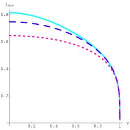
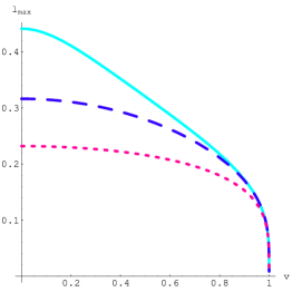
(a)	(b)	(c)

Figure 3: (a), (b) Plots of $\ell_{\rm max}(v)$ for the case of two angular momenta at $\theta={\pi\over 2}$ (with similar plots for $\theta=0$) with $\lambda=0.5$ and $\lambda=0.95$ respectively; The solid, dashed and dotted lines are as in Fig. 2(c). (c) Plot of the function $G(\xi)$ for the case of two angular momenta.

$\bullet$ For the case with $\theta=\pi/2$, we have the expression

$$\ell(v,\xi,y_{0})\ =\ G(\xi)\ {\sqrt{y_{0}^{4}-\gamma^{2}}\over y_{0}^{3}}\ \int_{1}^{\infty}{dz\over\sqrt{(z^{2}-1/y_{0}^{2})(z-\lambda^{2}/y_{0}^{2})(z^{2}-1)}}\ .$$ (4.18)

Performing a similar analysis as before we find that the various coefficients entering (1.1) are given by

$$c_{1}=0.2106\ ,\qquad c_{2}=0.100\ ,\qquad c_{3}=0.0898\ .$$ (4.19)

For ${\cal F}(v,\xi)$ we give its numerical values in the four corners in the $(v,\xi)$-plane

$${\cal F}(0,0)=1.06\ ,\qquad{\cal F}(0,\infty)=2.11\ ,\qquad{\cal F}(1,0)=1\ ,\qquad{\cal F}(1,\infty)=1\ ,$$ (4.20)

showing that it is a slowly-varying function except for the case of low velocity and extremely large R-charge. However, the region of the $(v,\xi)$ parameter space where these deviations from unity appear is very small, as can be easily verified by an explicit plot of ${\cal F}(v,\xi)$.

In both cases the function $G(\xi)$ is given by

$$G(\xi)=(1+F^{2})^{-1/2}=\sqrt{1-\lambda^{2}}\ .$$ (4.21)

It is plotted in Fig. 3(c) and it has a strong dependence on the dimensionless R-charge density $\xi$.

4.2.2 One nonzero angular momentum

Now, the functions $f_{y}(u)$ and $g(u)$ are given by

$$f_{y}(u)={1\over R^{4}}\left[u^{2}(u^{2}+r_{0}^{2}\cos^{2}\theta)-\gamma^{2}\mu^{4}\right]\ ,\quad g(u)={u^{2}(u^{2}+r_{0}^{2}\cos^{2}\theta)-\gamma^{2}\mu^{4}\over u^{2}(u^{2}+r_{0}^{2})-\mu^{4}}\ ,$$ (4.22)

and again the angular variable $\theta=0$ or $\theta={\pi\over 2}$ for consistency. The length integrals are given below.

$\bullet$ For the case with $\theta=0$ after a change of variables we find that

$$\ell(v,\xi,y_{0}) \!=\! G(\xi){\sqrt{y_{0}^{4}+\lambda^{2}y_{0}^{2}-\gamma^{2}}\over y_{0}^{3}}$$ (4.23)

$$\phantom{}\times\int_{1}^{\infty}{dz\over\sqrt{z(z-1)(z^{2}+\lambda^{2}z/y_{0}^{2}-1/y_{0}^{4})(z+1+\lambda^{2}/y_{0}^{2})}}\ .$$

An analysis similar to before gives for the numerical factors in (1.1) that

$$c_{1}=0.10525\ ,\qquad c_{2}=0.100\ ,\qquad c_{3}=-0.01507\ .$$ (4.24)

The numerical values of ${\cal F}(v,\xi)$ in the four corners of the $(v,\xi)$-plane are

$${\cal F}(0,0)=1.06\ ,\qquad{\cal F}(0,1.33)=1.05\ ,\qquad{\cal F}(1,0)=1\ ,\qquad{\cal F}(1,1.33)=1\ ,$$ (4.25)

showing again that it is indeed a very slowly varying function.

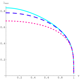
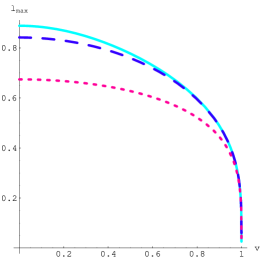
(a)	(b)	(c)

Figure 4: (a), (b) Plots of $\ell_{\rm max}(v)$ for the case of one angular momentum at $\theta=0$ (with similar plots for $\theta={\pi\over 2}$) with $\lambda=0.7$ and $\lambda=1.4$ respectively; the solid, dashed and dotted lines are as in Fig. 2(c). (c) Plot of the function $G(\xi)$ for the case of one angular momentum.

$\bullet$ For the case with $\theta=\pi/2$ we obtain after a similar variable change that

$$\ell(v,\xi,y_{0})=G(\xi){\sqrt{y_{0}^{4}-\gamma^{2}}\over y_{0}^{3}}\int_{1}^{\infty}{dz\over\sqrt{z(z^{2}-1)(z^{2}+\lambda^{2}z/y_{0}^{2}-1/y_{0}^{4})}}\ .$$ (4.26)

Now the numerical factor in (1.1) are

$$c_{1}=-0.2106\ ,\qquad c_{2}=0.100\ ,\qquad c_{3}=0.0898\ ,$$ (4.27)

while the numerical values of ${\cal F}(v,\xi)$ in the four corners of the $(v,\xi)$-plane are

$${\cal F}(0,0)=1.06\ ,\qquad{\cal F}(0,1.33)=0.74\ ,\qquad{\cal F}(1,0)=1\ ,\qquad{\cal F}(1,1.33)=1\ ,$$ (4.28)

showing that it is a slowly-varying function except for the case of low velocity with large R-charge when further corrections become important.

Now we have for the function $G(\xi)$ the expression

$$G(\xi)=F^{-3/4}(2-F)^{-1/4}=\sqrt{1+{\lambda^{4}\over 4}}\left(\sqrt{1+{\lambda^{4}\over 4}}-{\lambda^{2}\over 2}\right)^{1/2}\ .$$ (4.29)

This is depicted in Fig. 4(c) and shows a very weak dependence on the dimensionless R-charge density $\xi$.

One comment is in order here regarding the case of parallel motion having $\Theta=0$. In that case the form of the maximal screening length is the same with slightly different coefficients and function ${\cal F}$. The function $G(\xi)$ is the same and is independent of the angle $\Theta$, a fact that facilitates the computation of average values of the maximal screening lengths in the next section.

5 Plasma rest frame and averages

So far we have not considered the most general situation where the $q\bar{q}$-pair axis makes an arbitrary angle $\Theta$ with the velocity vector. A detailed investigation of this problem can be carried out either by numerical analysis of the full equations (2) or by an approximate analytic method that we will present here. We have already noted that the maximum separation length is a function of $\Theta$ through the combinations $\cos^{2}\Theta$ and $\sin^{2}\Theta$. Since its values for the extreme case $\Theta=0$ and $\Theta={\pi/2}$, do not differ very much, it is a good approximation for the screening length in the rest frame of the pair to write

$$L_{\rm max,q\bar{q}}(\Theta)=L_{\perp}\sin^{2}\Theta+L_{||}\cos^{2}\Theta\ ,$$ (5.1)

as it reduces to the above mentioned extreme cases, with the maximum screening lengths denoted by $L_{\perp}$ and $L_{||}$, in an obvious notation. It is of interest to know the average value of this length over all angles. To do that we have to know the probability for a $q\bar{q}$ pair to be moving at an angle, formed by its axis and its velocity vector, between $\Theta$ and $\Theta+d\Theta$. The most reasonable assumption is that this probability is uniform, but in the plasma rest frame. Denoting in the plasma rest frame by $\Theta^{\prime}$ the angle corresponding to the angle $\Theta$ in the $q\bar{q}$ rest frame, we have, due to length contraction in the direction $x$ parallel to the velocity vector, the relation

$$\tan\Theta^{\prime}=\gamma\tan\Theta\ ,$$ (5.2)

that is the length is not only contracted but also rotated. From these the useful relations

$$\cos^{2}\Theta^{\prime}={\gamma^{-2}\cos^{2}\Theta\over\gamma^{-2}\cos^{2}\Theta+\sin^{2}\Theta}\ ,\qquad\sin^{2}\Theta^{\prime}={\sin^{2}\Theta\over\gamma^{-2}\cos^{2}\Theta+\sin^{2}\Theta}$$ (5.3)

and their inverses

$$\cos^{2}\Theta={\gamma^{2}\cos^{2}\Theta^{\prime}\over\gamma^{2}\cos^{2}\Theta^{\prime}+\sin^{2}\Theta^{\prime}}\ ,\qquad\sin^{2}\Theta={\sin^{2}\Theta^{\prime}\over\gamma^{2}\cos^{2}\Theta^{\prime}+\sin^{2}\Theta^{\prime}}\ ,$$ (5.4)

follow. Then the probability distribution is

$$P_{\rm plasma}(\Theta^{\prime})d\Theta^{\prime}={2\over\pi}d\Theta^{\prime}={2\over\pi\gamma}{d\Theta\over\gamma^{-2}\cos^{2}\Theta+\sin^{2}\Theta}=P_{q\bar{q}}(\Theta)d\Theta\ .$$ (5.5)

Then the average value of the maximal screening length in the $q\bar{q}$-pair rest frame is

$$\bar{L}_{\rm max,q\bar{q}} = {2\over\pi\gamma}\int_{0}^{\pi/2}d\Theta\ {L_{\perp}\sin^{2}\Theta+L_{||}\cos^{2}\Theta\over\gamma^{-2}\cos^{2}\Theta+\sin^{2}\Theta}$$ (5.6)

$$= {L_{\perp}+\gamma L_{||}\over 1+\gamma}\ =\ L_{\parallel}+(L_{\perp}-L_{\parallel})\left({1\over\gamma}-{1\over\gamma^{2}}\right)+{\cal O}\left(1\over\gamma^{3}\right)\ .$$

This is essentially of the form (1.1) and for large enough $\gamma$ it is basically controlled by the maximal screening length $L_{\parallel}$ along the pair’s velocity vector. The reason for this is the fact that the probability (5.5), although uniform in the plasma rest frame, it is peaked at $\Theta=0$ with a width of order $1/\gamma$, in the $q\bar{q}$-pair rest frame.

In the plasma rest frame the expression corresponding to (5.1) differs from the above in that we have to take into account the Lorentz contraction of the component of the separation length vector parallel to the velocity. We find

$$L_{\rm max,plasma}(\Theta^{\prime}) = (L_{\perp}\sin^{2}\Theta+L_{||}\cos^{2}\Theta)\sqrt{\gamma^{-2}\cos^{2}\Theta+\sin^{2}\Theta}$$ (5.7)

$$= {L_{\perp}\sin^{2}\Theta^{\prime}+L_{||}\gamma^{2}\cos^{2}\Theta^{\prime}\over(\gamma^{2}\cos^{2}\Theta^{\prime}+\sin^{2}\Theta^{\prime})^{3/2}}\ ,$$

with average

$$\bar{L}_{\rm max,plasma} = {2\over\pi\gamma}\int_{0}^{\pi/2}d\Theta\ {L_{\perp}\sin^{2}\Theta+L_{||}\cos^{2}\Theta\over\sqrt{\gamma^{-2}\cos^{2}\Theta+\sin^{2}\Theta}}$$ (5.8)

$$= {2\over\pi\gamma}\left[L_{\perp}+L_{\parallel}\ln(4e^{-1}\gamma)\right]+{\cal O}\left(1\over\gamma^{3}\right)\ .$$

We see that there is a $1/\gamma$ suppression of the maximal screening length, the reason being, as explained before, that in the pair’s rest frame the production is peaked near $\Theta=0$. The presence of the $\ln\gamma$ term in the overall coefficient is due to the contribution of the integral in the region near $\Theta=0$. The last expression in the basis of our proposal for a maximum screening length in the plasma rest frame in (1.3).

We note for completeness that, if we take the angle distribution to be uniform in the $q\bar{q}$-pair rest frame, then the average value of the maximum length in the rest frame of the pair would be, instead of (5.6)

$$\bar{L}_{\rm max,q\bar{q}}={L_{\perp}+L_{||}\over 2}\ ,$$ (5.9)

again of the form (1.1). Also the corresponding average in the plasma rest frame would be

$$\bar{L}_{\rm max,plasma} = {2\over\pi}\int_{0}^{\pi/2}d\Theta\ (L_{\perp}\sin^{2}\Theta+L_{||}\cos^{2}\Theta)\sqrt{\gamma^{-2}\cos^{2}\Theta+\sin^{2}\Theta}$$

$$= {1\over 2}\left[L_{\perp}\ {}_{2}F\!_{1}(-{1\over 2},{1\over 2},2,v^{2})+L_{\parallel}\ {}_{2}F\!_{1}(-{1\over 2},{3\over 2},2,v^{2})\right]$$

$$= {2\over 3\pi}(2L_{\perp}+L_{\parallel})+{1\over 6\pi\gamma^{2}}\Big{(}2L_{\perp}-5L_{\parallel}+6L_{\parallel}\ln(4\gamma)\Big{)}+{\cal O}\left(1\over\gamma^{4}\right)\ .$$

The last expression is the basis of our second possibility, less likely in our opinion, for a maximum screening length in the plasma rest frame in (1.4).

Acknowledgments

K. S. would like to thank U. Wiedemann for a useful discussion, as well as the Theory-Division at CERN and the Institute of Physics of the University of Neuchâtel for hospitality and financial support during a considerable part of this research. K. S. also acknowledges the support provided through the European Community’s program “Constituents, Fundamental Forces and Symmetries of the Universe” with contract MRTN-CT-2004-005104, the INTAS contract 03-51-6346 “Strings, branes and higher-spin gauge fields”, the Greek Ministry of Education programs $\rm\Pi Y\Theta A\Gamma OPA\Sigma$ with contract 89194 and the program $\rm E\Pi AN$ with code-number B.545.

References

- [1]
- [2] J.M. Maldacena, Adv. Theor. Math. Phys. 2 (1998) 231, Int. J. Theor. Phys. 38 (1999) 1113, hep-th/9711200. S.S. Gubser, I.R. Klebanov and A.M. Polyakov, Phys. Lett. B428 (1998) 105, hep-th/9802109. E. Witten, Adv. Theor. Math. Phys. 2 (1998) 253, hep-th/9802150 and Adv. Theor. Math. Phys. 2 (1998) 505, hep-th/9803131.
- [3] J.M. Maldacena, Phys. Rev. Lett. 80 (1998) 4859, hep-th/9803002. S.J. Rey and J.T. Yee, Eur. Phys. J. C22 (2001) 379, hep-th/9803001.
- [4] S.J. Rey, S. Theisen and J.T. Yee, Nucl. Phys. B527 (1998) 171, hep-th/9803135. A. Brandhuber, N. Itzhaki, J. Sonnenschein and S. Yankielowicz, Phys. Lett. B434 (1998) 36, hep-th/9803137 and JHEP 9806 (1998) 001, hep-th/9803263.
- [5] A. Brandhuber and K. Sfetsos, Adv. Theor. Math. Phys. 3 (1999) 851, hep-th/9906201.
- [6] J.C. Collins and M.J. Perry, Phys. Rev. Lett. 34 (1975) 1353. E.V. Shuryak, Phys. Lett. B78 (1978) 150 [Sov. J. Nucl. Phys. 28 (1978) 408].
- [7] E. Shuryak, Prog. Part. Nucl. Phys. 53 (2004) 273, hep-ph/0312227, Nucl. Phys. A750 (2005) 64, hep-ph/0405066 and Strongly coupled quark-gluon plasma: The status report, hep-ph/0608177. M. J. Tannenbaum, Rept. Prog. Phys. 69 (2006) 2005, nucl-ex/0603003.
- [8] G. Policastro, D.T. Son and A.O. Starinets, Phys. Rev. Lett. 87 (2001) 081601, hep-th/0104066, JHEP 0209 (2002) 043, hep-th/0205052 and JHEP 0212 (2002) 054, hep-th/0210220. A. Buchel, J.T. Liu and A.O. Starinets, Nucl. Phys. B707 (2005) 56, hep-th/0406264.
- [9] C.P. Herzog, A. Karch, P. Kovtun, C. Kozcaz and L.G. Yaffe, JHEP 0607 (2006) 013, hep-th/0605158. S.S. Gubser, Drag force in AdS/CFT, hep-th/0605182.
- [10] C.P. Herzog, JHEP 0609(2006) 032, hep-th/0605191. E. Cáceres and A. Guijosa, JHEP 0611 (2006) 077, hep-th/0605235.
- [11] J.J. Friess, S.S. Gubser and G. Michalogiorgakis, JHEP 0609 (2006) 072, hep-th/0605292. J.J. Friess, S.S. Gubser, G. Michalogiorgakis and S.S. Pufu, The stress tensor of a quark moving through N = 4 thermal plasma, hep-th/0607022.
- [12] H. Liu, K. Rajagopal and U.A. Wiedemann, Phys. Rev. Lett. 97 (2006) 182301, hep-ph/0605178.
- [13] A. Buchel, Phys. Rev. D74 (2006) 046006, hep-th/0605178. J.F. Vázquez-Poritz, Enhancing the jet quenching parameter from marginal deformations, hep-th/0605296. E. Cáceres and A. Guijosa, On Drag Forces and Jet Quenching in Strongly Coupled Plasmas, hep-th/0606134.
- [14] J. Casalderrey-Solana and D. Teaney, Phys. Rev. D74 (2006) 085012, hep-ph/0605199.
- [15] S.D. Avramis and K. Sfetsos, Supergravity and the jet quenching parameter in the presence of R-charge densities, hep-th/0606190.
- [16] N. Armesto, J.D. Edelstein and J. Mas, JHEP 0609 (2006) 039, hep-ph/0606245.
- [17] F.L. Lin and T. Matsuo, Phys. Lett. B641 (2006) 45, hep-th/0606136.
- [18] T. Matsui and H. Satz, Phys. Lett. B178 (1986) 416.
- [19] F. Karsch, M.T. Mehr and H. Satz, Z. Phys. C37, 617 (1988).
- [20] M.C. Chu and T. Matsui, Phys. Rev. D39 (1989) 1892.
- [21] K. Peeters, J. Sonnenschein and M. Zamaklar, Phys. Rev. D74 (2006) 106008, hep-th/0606195.
- [22] H. Liu, K. Rajagopal and U.A. Wiedemann, An AdS/CFT calculation of screening in a hot wind, hep-ph/0607062.
- [23] M. Chernicoff, J.A. Garcia and A. Guijosa, JHEP 0609 (2006) 068, hep-th/0607089.
- [24] P.C. Argyres, M. Edalati and J.F. Vázquez-Poritz, No-Drag String Configurations for Steadily Moving Quark-Antiquark Pairs in a Thermal Bath, hep-th/0608118.
- [25] E. Cáceres, M. Natsuume and T. Okamura, JHEP 0610 (2006) 011, hep-th/0607233.
- [26] R. Hernandez, K. Sfetsos and D. Zoakos, JHEP 0603 (2006) 069, hep-th/0510132.
- [27] H. Liu, K. Rajagopal and U.A. Wiedemann, to appear. Private communication with U.A. Wiedemann.
- [28] P. Kraus, F. Larsen and S.P. Trivedi, JHEP 9903 (1999) 003, hep-th/9811120.
- [29] M. Cvetic and D. Youm, Nucl. Phys. B477 (1996) 449, hep-th/9605051.
- [30] J.G. Russo and K. Sfetsos, Adv. Theor. Math. Phys. 3 (1999) 131, hep-th/9901056.
- [31] S.S. Gubser, Nucl. Phys. B551 (1999) 667, hep-th/9810225. R.G. Cai and K.S. Soh, Mod. Phys. Lett. A14 (1999) 1895, hep-th/9812121. M. Cvetic and S.S. Gubser, JHEP 9907 (1999) 010, hep-th/9903132. T. Harmark and N.A. Obers, JHEP 0001 (2000) 008, hep-th/9910036.