Entanglement and Nonunitary Evolution

Abstract:

We consider a collapsing relativistic spherical shell for a free quantum field. Once the center of the wavefunction of the shell passes a certain radius $r_{s}$, the degrees of freedom inside $r_{s}$ are traced over. We show that an observer outside this region will determine that the evolution of the system is nonunitary. We argue that this phenomenon is generic to entangled systems, and discuss a possible relation to black hole physics.

1 Introduction

Consider a free massless scalar field in a pure state $|\psi\rangle$ describing a spherically symmetric inward collapsing shell. Imagine that once the shell reaches a certain radius $r_{s}$, an observer located at $r>r_{s}$ has no access to the region $r<r_{s}$. This implies that the state seen by this outside observer is a mixed state described by the density matrix $\rho_{out}=\text{Tr}_{r<r_{s}}|\psi\rangle\langle\psi|$. We shall investigate the time evolution of the state $\rho_{out}$.

There are general arguments, which we discuss below, that show that a generic entangled state will seem to evolve in a nonunitary way if part of the Hilbert space is inaccessible—a property that leads to dissipation effects in many body systems. In this paper, we shall show that the eigenvalues of $\rho_{out}$ are time dependent. This implies that $\rho_{out}$ does not evolve in a unitary manner (see figure 1). To see this, consider a quantum system prepared in an initial state defined by the density matrix $\rho(0)$. If the evolution is unitary, then the density matrix $\rho(t)$ describing the system at a later time is related to $\rho(0)$ by $\rho(t)=U^{\dagger}(t)\rho(0)U(t)$. Since this is a similarity transformation, the eigenvalues of $\rho(t)$ must be the same as those of $\rho(0)$, and are consequently time-independent. Conversely, consider a density matrix $\rho(t)$ whose eigenvalues are time dependent. In this case, for the same reason, a unitary operator $U(t)$ such that $\rho(t)=U^{\dagger}(t)\rho(0)U(t)$ does not exist. Therefore, the time evolution of a system will be unitary if and only if the eigenvalues of $\rho$ are time independent.

Previous investigations of the relationship between entanglement, entropy and area [1] have shown that the von Neumann entropy $S=\text{Tr}_{r>r_{s}}(\rho_{out}\ln\rho_{out})$ of an initial vacuum state $|0\rangle$ is proportional to the surface area of the region $r<r_{s}$, suggesting a connection with black hole entropy. This observation (see also [2]) has been studied in the literature from various perspectives [3, 4, 5, 6, 7, 8, 9, 10, 11, 12, 13, 14, 15, 16, 17, 18, 19] (see [20, 21] for a review). In flat space, it can be shown that the entropy (and other thermodynamic quantities) will scale as the surface area of the inaccessible volume even when it is nonspherical [12, 15, 13]. This area dependence may be related to thermodynamic properties of Unruh radiation [22, 23].

The flat space arguments relating entanglement entropy and area may be extended to a black hole background [24, 25, 26]. Since this work is key in understanding the relation between our results to black hole evolution, we shall briefly review it. Consider, for simplicity, an eternal uncharged and non rotating black hole. This black hole has two asymptotic regions separated by a horizon. As a result of this causal structure, an observer in one asymptotic region has no access to the degrees of freedom in the other asymptotic region. In contrast, the global vacuum of this system (the Hartle-Hawking vacuum) extends to both asymptotic regions. An observer in one asymptotic region will observe the state obtained from the vacuum after degrees of freedom in the other asymptotic region are traced over—the degrees of freedom “behind” the horizon. The resultant state is not a pure state but rather a mixed state which turns out to be precisely the density matrix seen by an observer restricted to one asymptotic region at the Hawking temperature. As in the flat space case, the entropy associated with this state is proportional to the surface area of the horizon. This mechanism, which is a result of the entangled nature of the vacuum state, allows one to interpret the black hole entropy as coming from entanglement, an interpretation which is consistent with the string theory evaluation of black hole entropy [26, 27, 28, 29, 30] (see also [31, 32, 33, 34, 35, 36, 37] for a recent discussion of black hole entropy and entanglement in the context of AdS/CFT.)

Thus, following [1], the current work is a natural next step in relating features of entanglement to black hole physics. While it is generally believed that black holes have entropy proportional to their surface area [38] there is, at the moment, some debate regarding their time evolution.

In [39] it was argued that the evolution in time of a black hole is nonunitary (see [40, 41, 42, 43, 44, 45, 46, 47, 48, 49, 50] for recent discussions and implications). This is a troubling feature of black holes since it clashes with our understanding of quantum mechanics. For instance, if the evolution is nonunitary a pure state (for which the density matrix has a single nontrivial eigenvalue) may evolve into a mixed state. From the entanglement point of view this behavior is not in contradiction with the principles of quantum mechanics or any laws of physics, rather it is a simple consequence of the entangled nature of the system. If one does not have access to part of the Hilbert space then probability flowing into the inaccessible region will seem to disappear leading to nonunitary evolution.

2 General arguments

There are several approaches one may take when trying to exhibit the nonunitary evolution of an entangled system. Many of these have been studied in the context of dissipation of energy from a system to a heat bath (see for example [51] and references therein) and may be directly applied to our discussion. We review them here for completeness.

We would like to exhibit the nonunitary evolution of an initial pure state $\rho(0)=|\psi\rangle\langle\psi|$ seen by an observer who has no access to a certain region of space. We evolve our initial state in time using the Liouvillian operator $\mathcal{L}=-\imath[H,\quad]$, so that $\dot{\rho}(t)=\mathcal{L}\rho(t)$.

We shall split our Hilbert space of states into two parts, which we will refer to as the ‘in’ region and the ‘out’ region, such that the Hamiltonian can be written as $H=H_{out}+H_{I}+H_{in}$ with $H_{I}$ an interaction term. Since $\mathcal{L}$ is linear, this correspondingly results in $\mathcal{L}=\mathcal{L}_{out}+\mathcal{L}_{I}+\mathcal{L}_{in}$.

Consider an observer restricted to, say, the ‘out’ region of space, and let $R$ be an operator that restricts the density matrix to this region. This corresponds to “integrating out” the unobservable degrees of freedom. (In the path integral formalism, $R$ is given by eq. (4) below.) We assume that the ‘in’ and ‘out’ regions are fixed, so that $R$ is time-independent (though a generalization to a time dependent $R$ is straightforward).

Suppose that at some time $t=0$ the state of the observer is given by $\rho_{out}(0)=R\rho(0)$. The state $\rho_{out}$ will then evolve in time according to $\dot{\rho}_{out}(t)=R\dot{\rho}(t)$. Note that, once we restrict observables to the ‘out’ region, a further restriction will not change the state of the system, therefore $R^{2}=R$.

To find $\dot{\rho}_{out}$, we act, in turn, with $(I-R)$ and $R$ on $\dot{\rho}=\mathcal{L}\rho_{out}+\mathcal{L}(I-R)\rho$, obtaining equations for $\dot{\rho}_{out}$ and $(I-R)\dot{\rho}$. Plugging the (formal) solution to $(I-R)\rho$ into the equation for $\rho_{out}$ we obtain the Nakajima-Zwanzig [52, 53, 54] form of the master equation

$$\dot{\rho}_{out}(t)= \left(R\mathcal{L}\right)\rho_{out}(t)+\int_{0}^{t}\left(R\mathcal{L}\right)\big{|}_{t}\exp\left[\int_{t-\bar{t}}^{t}\left((I-R)\mathcal{L}\right)dt^{\prime}\right]\left((I-R)\mathcal{L}\right)\rho_{out}\big{|}_{t-\bar{t}}d\bar{t}+$$

$$+\left(R\mathcal{L}\right)\big{|}_{t}\exp\left(\int_{0}^{t}(I-R)\mathcal{L}dt^{\prime\prime}\right)(I-R)\rho(0).$$ (1)

To simplify (1) we note that the restriction $R$ commutes with time evolution in the ‘in’ and ‘out’ regions $[R,\mathcal{L}_{out}]=[R,\mathcal{L}_{in}]=0$. Also, we assume that, $\mathcal{L}_{in}R=0$. Finally, since $R\exp\left[\int_{t-\bar{t}}^{t}\left((I-R)\mathcal{L}\right)dt^{\prime}\right]\left((I-R)\mathcal{L}_{I}\right)(t-\bar{t})=0$, we find

$$\dot{\rho}_{out}(t)= R(\mathcal{L}_{out}+\mathcal{L}_{I})\rho_{out}(t)+$$

$$+\int_{0}^{t}\left(R\mathcal{L}_{I}\right)\big{|}_{t}\exp\left[\int_{t-\bar{t}}^{t}\left((I-R)\mathcal{L}\right)dt^{\prime}\right]\left((I-R)\mathcal{L}_{I}\right)\rho_{out}\big{|}_{t-\bar{t}}d\bar{t}+$$

$$+R\mathcal{L}_{I}(t)\exp\left(\int_{0}^{t}(I-R)\mathcal{L}dt^{\prime\prime}\right)(I-R)\rho(0).$$ (2)

The first term in eq. (2) is the standard term that one expects for unitary time evolution of the state seen by the observer in the ‘out’ region. The second term represents the (time retarded) oscillations flowing into the ‘out’ region from the ‘in’ region that is being traced over (“beyond the horizon”). The last term represents contributions leaking out of the inaccessible region from those initially present. In most many-body applications, it is arranged or assumed that $(I-R)\rho(0)\approx 0,$ so that this term can be neglected.

The interaction term in the Hamiltonian, $H_{I}$, is essential for generating the nonunitary evolution. In a field theory setting, this interaction term includes the spatial derivative coupling fields across the boundary. Thus, it exists even for a free field theory.

3 Explicit construction of nonunitary evolution.

We wish to explicitly exhibit the nonunitary evolution measured by an observer who does not have access to part of a system. Consider the time evolution of an inward collapsing spherical shell of a free massless field in $3+1$ dimensions from the point of view of an observer who does not have access to the region $r<r_{s}$. We choose such a configuration for two reasons: (a) to make suggestive contact with gravitational collapse, and (b) since any choice of an initial state that is an eigenstate of the Hamiltonian (such as the vacuum state) will not exhibit any time evolution due to its stationary nature.

Let $\Psi_{k}[\phi(\vec{x})]$ be the wavefunctional of a single particle with energy $E_{k}=|\vec{k}|$ of a free massless scalar field $\phi(\vec{x})$ in three space dimensions. An arbitrary configuration $\Psi$ for such a particle is specified by $\Psi=\sum_{k}f_{k}\Psi_{k}$. We construct a collapsing shell by choosing $\{f_{k}\}$ such that only s-wave modes are excited and such that the initial position space wavefunction is centered at some radius $r_{i}$ and is collapsing toward the origin. To obtain $f_{k}$ explicitly, consider the wavefunction

$$|\psi\rangle=A^{-1/2}\int\hat{f}(r)\phi(\vec{x})|0\rangle d^{3}x$$ (3)

where $A$ is a normalization constant determined by the condition $\langle\psi|\psi\rangle=1$ and $\hat{f}(r)$ is real. The average momentum of the shell, $p$, is set by substituting $\hat{f}(r)\to e^{\imath pr}\hat{f}(r)$. The set $\{f_{k}\}$ may be obtained from the expansion of the field $\phi$ in terms of ladder operators.

The density matrix of the region seen by an observer in the exterior is given by

$$\rho_{out}(\phi_{out},\phi^{\prime}_{out})=\int D\phi_{in}\Psi(\phi_{in},\phi_{out})\Psi(\phi_{in},\phi^{\prime}_{out})^{\dagger}.$$ (4)

A similar density matrix was constructed in a somewhat different context in [55].

As in [1, 6], one can calculate the functional integral (4) by discretizing space on a radial lattice. We expand the scalar field $\phi$ in partial wave components

$$\phi_{l,m}(r)=r\int Z_{lm}(\theta,\varphi)\phi(\vec{x})d\Omega,\qquad\pi_{l,m}(r)=r\int Z_{lm}(\theta,\varphi)\pi(\vec{x})d\Omega,$$ (5)

where $r=|\vec{x}|$ and $Z_{0,0}=Y_{0,0}$, $Z_{l,m}=\sqrt{2}\text{Re}Y_{l,m}$ for $m>0$, and $Z_{l,m}=\sqrt{2}\text{Im}Y_{l,m}$ for $m<0$. $Z_{l,m}$ are orthonormal and complete. This allows us to write the Hamiltonian as $H=\sum H_{l,m}$ with

$$H_{l,m}=\frac{1}{2}\int_{0}^{\infty}dr\left[\pi_{l,m}^{2}(r)+r^{2}\left(\partial_{r}\left(\frac{\phi_{l,m}(r)}{r}\right)\right)^{2}+\frac{l(l+1)}{r^{2}}\phi_{l,m}^{2}(r)\right].$$ (6)

We discretize the radial coordinate on a lattice of spacing $a$ and of size $L=(N+1)a$ with boundary conditions such that the fields vanish at $r=L$. The expressions for the $H_{l,m}$’s (6) become those of Hamiltonians of coupled harmonic oscillators.

$$H_{l,m} =\frac{1}{2a}\sum_{j=1}^{N}\left[\pi_{l,m,j}^{2}+(j+\frac{1}{2})^{2}\left(\frac{\phi_{l,m,j}}{j}-\frac{\phi_{l,m,j+1}}{j+1}\right)^{2}+\frac{l(l+1)}{j^{2}}\phi_{l,m,j}^{2}\right]$$

$$\equiv\frac{1}{2a}\left(\pi^{2}+\phi K_{l,m}\phi\right).$$ (7)

Note that all the oscillators are coupled due to the spatial derivatives of the field. This coupling generates the interaction Hamiltonian described earlier.

The wavefunction for a single particle shell is constructed as in the continuum (3)

$$|\psi\rangle=\frac{a^{2}}{A^{1/2}}\sum_{i=1}^{N}i\hat{f}_{i}\phi_{0,0,i}|0\rangle.$$ (8)

We wish to write this in a single particle eigenbasis of the Hamiltonian $\{a_{i}^{\dagger}|0\rangle\}_{i=1}^{N}$. Let $y_{i}=S^{0}_{ij}\phi_{0,0,j}$, where $S^{0}$ diagonalizes $K_{0,0}$ defined in (7). We find that

$$|\psi\rangle =A^{-1/2}\frac{1}{\sqrt{2}}\sum_{j,k=1}^{N}j\hat{f}_{j}S^{0}_{kj}(\Omega^{0}_{k,k})^{-\frac{1}{2}}a_{k}^{\dagger}|0\rangle$$ (9)

with

$$A =\frac{1}{2}\sum_{j,j^{\prime}}j^{\prime}\hat{f}_{j^{\prime}}\left(K_{0,0}^{-1/2}\right)_{j^{\prime}j}j\hat{f}_{j}.$$

In (9) we have defined $(\Omega^{0})^{2}=S^{0}K_{0,0}S^{0\,T}$. As in the continuum, one can generate a collapsing shell by substituting $\hat{f}_{j}\to e^{\imath kj}\hat{f}_{j}$. The time dependence of the state $|\psi\rangle$ can be read off from $|\psi,t\rangle=e^{-\imath Ht}|\psi\rangle$

The wavefunctional on this discretized space is given by

$$\Psi_{k}(\{\phi_{l,m,j}\})=\frac{N_{0}}{\sqrt{2}}H_{1}(\sqrt{\omega_{k}}y_{k})e^{-\frac{1}{2}y\Omega y}$$

with $N_{0}=\frac{\omega^{\frac{1}{4}}}{\sqrt{\pi^{\frac{1}{2}}}}$, $y=S\phi$ where $S$ diagonalizes $K$, $(K)^{\alpha}=S^{T}(\Omega)^{2\alpha}S$ and $H_{1}(x)=2x$ is a Hermite Polynomial. In what follows it will be useful to compare our results to those obtained by studying the ground state wavefunctional

$$\Psi_{0}(\{\phi_{l,m,j}\})=N_{0}e^{-\frac{1}{2}y\Omega y}.$$ (10)

We shall consider a general linear superposition of single excited oscillators

$$\Psi =\sum_{k}f_{k}\Psi_{k}$$ (11)

$$=\frac{N_{0}}{\sqrt{2}}\left(2\phi S^{T}\Omega^{\frac{1}{2}}f\right)e^{-\frac{1}{2}\phi K^{\frac{1}{2}}\phi}.$$ (12)

For convenience, we define

$$v_{k}=\left(f\Omega^{\frac{1}{2}}S\right)_{k}.$$ (13)

Note that $v_{n}=A^{-\frac{1}{2}}\sum_{j}jf_{j}(e^{-\imath Ht})_{j,n}$. This allows us to write $\rho_{out}=\int\psi\psi^{\star}d\phi_{in}$ as

$$\rho_{out}(w,w^{\prime})=2\int(v\cdot\phi)(v^{\star}\cdot\phi^{\prime})|N_{0}|^{2}e^{-\frac{1}{2}\phi K^{\frac{1}{2}}\phi}e^{-\frac{1}{2}\phi^{\prime}K^{\frac{1}{2}}\phi^{\prime}}d^{n}z,$$ (14)

where we have used $\phi=\begin{pmatrix}z,w\end{pmatrix}$, and $\phi^{\prime}=\begin{pmatrix}z,w^{\prime}\end{pmatrix}$.

The right-hand-side of eq. (14) is a Gaussian integral over the first $n$ coordinates. Using the notation

$$v=\begin{pmatrix}v_{1}\\ v_{2}\end{pmatrix},\quad K^{\frac{1}{2}}=\begin{pmatrix}A&B\\ B^{T}&C\end{pmatrix},$$ (15)

we find

$$\rho_{out}(w,w^{\prime})= 2\rho_{0,out}(w,w^{\prime})\times$$

$$\times\Bigg{(}\left(\frac{1}{2}v_{1}A^{-1}B(w+w^{\prime})\right)\left(\frac{1}{2}v_{1}^{\star}A^{-1}B(w+w^{\prime})\right)+\frac{1}{2}v_{1}A^{-1}v_{1}^{\star}-$$

$$\phantom{\times\Bigg{(}}-(v_{2}\cdot w)\frac{1}{2}v_{1}^{\star}A^{-1}B(w+w^{\prime})-(v_{2}^{\star}\cdot w^{\prime})\frac{1}{2}v_{1}A^{-1}B(w+w^{\prime})+$$

$$\phantom{\times\Bigg{(}}+(v_{2}\cdot w)(v_{2}^{\star}\cdot w^{\prime})\Bigg{)},$$ (16)

where

$$\rho_{0,out}(w,w^{\prime})=|N_{0}|^{2}\frac{\pi^{\frac{n}{2}}}{|A|^{\frac{1}{2}}}\exp\left(\frac{1}{4}(w+w^{\prime})B^{T}A^{-1}B(w+w^{\prime})-\frac{1}{2}(wCw+w^{\prime}Cw^{\prime})\right)$$ (17)

is the density matrix corresponding to the vacuum state (10). One can check that $\text{Tr}\rho_{0,out}=\text{Tr}\rho_{out}=1$.

The eigenvalues of $\rho_{0,out}$ may be obtained numerically [1] (see also [11] for an analytic approach). An approximation for the eigenvalues of the first excited state has been discussed in [6]. Since we are interested in exhibiting the nonunitary time evolution of the state measured by an external observer at $r>r_{s}$, we shall evaluate $\text{Tr}(\rho_{out}^{2})$; if $\text{Tr}(\rho_{out}^{2})$ is time dependent then, since $\text{Tr}(\rho_{out})=1$, at least two of its eigenvalues are time dependent.

To calculate $\text{Tr}(\rho_{out}^{2})$ we carry out another Gaussian integral. For the ground state we find

$$\text{Tr}(\rho_{0,out}^{2})=\frac{|K|}{|A||\Upsilon|^{\frac{1}{2}}},$$ (18)

where we have defined

$$\Upsilon=\begin{pmatrix}C-\frac{1}{2}B^{T}A^{-1}B&-\frac{1}{4}B^{T}A^{-1}B\\ -\frac{1}{4}B^{T}A^{-1}B&C-\frac{1}{2}B^{T}A^{-1}B\end{pmatrix}.$$ (19)

If $K$ were block diagonal such that $B=0$, then we would have had $|\Upsilon|=|C|^{2}$, so that $\text{Tr}(\rho_{0,out}^{2})=1$. We expect this since $B=0$ implies that the ‘in’ and ‘out’ oscillators are not entangled.

For our collapsing shell (9) we find, after some algebra, that

$$\text{Tr}(\rho_{out}^{2})=\left[\left(v\left[\begin{pmatrix}A^{-1}&0\\ 0&0\end{pmatrix}+U_{B}\right]v^{\star}\right)^{2}\\ +\left(vU_{A}v^{\star}\right)^{2}+\left|vU_{B}v\right|^{2}\right]\text{Tr}(\rho_{0,out}^{2})$$ (20)

where

$$U_{A/B}=\begin{pmatrix}\frac{1}{4}A^{-1}B(o_{A}+o_{B})B^{T}A^{-1}&-\frac{1}{2}A^{-1}B(o_{A}+o_{B})\\ -\frac{1}{2}(o_{A}+o_{B})B^{T}A^{-1}&o_{A/B}\end{pmatrix}$$ (21)

and $o_{A}$ and $o_{B}$ are defined through

$$\Upsilon^{-1}=\begin{pmatrix}o_{A}&o_{B}\\ o_{B}&o_{A}\end{pmatrix}$$ (22)

(where $\Upsilon$ is given in (19), and the block matrices $A,B$ and $C$ are given in (15)). As in the ground state case, one may check that $\text{Tr}(\rho_{out}^{2})=1$ if $B=0$.

In principle, the time dependence of $\rho_{out}$ can be extracted from (20). It is clear that if $f$ (recall $v=f\Omega^{1/2}S$) has a single entry (implying that the state of the system is an energy eigenstate) then $\text{Tr}(\rho_{out}^{2})$ will be time independent. The same applies to the ground state $\text{Tr}(\rho_{0,out}^{2})$ (18). In fact, as discussed earlier, any stationary state will generate a time independent $\rho_{out}$, meaning that the time evolution will be unitary. (Curiously, the same applies to coherent states (see [6]).) To obtain the time dependence of $\text{Tr}(\rho_{out}^{2}),$ we shall resort to numerical methods.

In figure 1, we have plotted the radial wavefunction $\sum_{j}jf_{j}(e^{-\imath Ht})_{j,n}$ as a function of the lattice location, $n$, and time, $t$, for the time interval $[4a,15a]$. We used a radial lattice of size $N+1=50$. The initial wavefunction was chosen such that at $t=0$ it is a Gaussian shell localized at $r_{s}=33a$ with width $\sigma=\sqrt{5}a$, and momentum $-1a$. The thick (red) line specifies the location of the maximum of the wavefunction. Once the center of the wavefunction passes $r_{s}=25a$ (at $t=8.84a$) we trace over the region $r<r_{s}$. In the figure, this region is bounded by a semi-transparent membrane. The value of $\text{Tr}(\rho_{out}^{2})$ at $t>8.84a$ is also plotted.

As the wavefunction enters the inaccessible region $r<25a$, $\text{Tr}(\rho_{out}^{2})$ starts increasing. This increase is to be expected: once the wavefunction is ‘almost’ completely inside the region $r<r_{s},$ then the one particle excitation of the density matrix $\rho_{in}$ would describe an ‘almost’ pure state implying $\text{Tr}(\rho_{in}^{2})/\text{Tr}(\rho_{0,in}^{2})=1$. Since $\rho_{in}$ and $\rho_{out}$ have equal eigenvalues (up to zeros), we get the behavior depicted in the plot.

If the tracing procedure is carried out before $t=8.84a$, then one finds that $\text{Tr}(\rho_{out}^{2})/\text{Tr}(\rho_{0,out}^{2})$ drops smoothly from $\sim 1$ (when the wavefunction is localized at $r>r_{s}$) to $\sim 0.4$ at $t\sim 8.8a$. Similarly, one can extend the analysis to $t>15a,$ whence the wavefunction “bounces back” from the origin: as the wavefunction leaves the $r>r_{s}$ region, another sharp change in $\text{Tr}(\rho_{out}^{2})/\text{Tr}(\rho_{0,out}^{2})$ is noted. At very long time scales, the wavefunction will bounce back and forth from the origin and IR boundary of space. In this case one will find a semi-periodic behavior for $\text{Tr}(\rho_{out}^{2})$. In general, we observe that $\text{Tr}(\rho_{out}^{2})=\alpha(t)\text{Tr}(\rho_{0,out}^{2})$ (see eq. (20)), where the coefficient $\alpha$ approaches unity when the wavefunction is localized either in the $r<r_{s}$ region or when it is localized in the $r>r_{s}$ region.

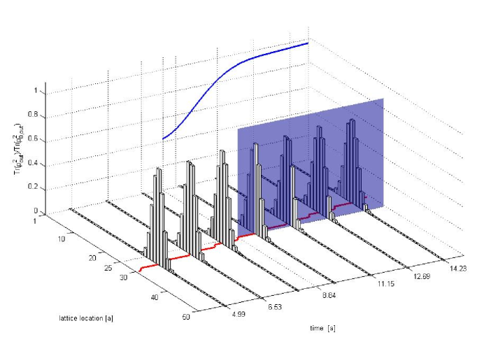
Figure 1: A plot of the radial component of a collapsing spherical wavefunction as a function of the lattice location, $n$, and time, $t$. The radial lattice has $50$ points of spacing $a$. At $t=0$ the wavefunction is a Gaussian shell localized at $33a$ with width $\sigma=\sqrt{5}a$, and momentum $-1/a$. The thick (red) line specifies the location of the maximum of the wavefunction. Once the center of the wavefunction passes $r_{s}=25a$ (at $t=8.84a$) we trace over the region $r<r_{s}$ (bounded by a semi-transparent membrane). $\frac{\text{Tr}(\rho_{out}^{2})}{\text{Tr}(\rho_{0,out}^{2})}$ is also plotted for $t>8.84a$.

We point out that since the wavefunctions corresponding to $\phi_{0,0,j}|0\rangle$ are orthogonal under the Klein Gordon norm then they are not orthogonal under the Dirac norm. Therefore, the plot only gives a suggestive description of the region where the wavefunction is localized. Also, since the scalar field is massless, a zero momentum s-wave will split into an outgoing shell and an ingoing shell. The amplitude of the outgoing shell is small initially because the wavefunction has been given a large initial ingoing momentum.

4 Discussion

The main point of this exercise is to emphasize that nonunitary time evolution of a density matrix is an ubiquitous phenomenon and does not signify a breakdown either of unitarity or of quantum mechanics. Whenever an observer has a limited domain of observation, she will describe observables in terms of a density matrix resulting from tracing over states outside that domain [56]. If her states are entangled with states beyond her domain, then she will experience a density matrix corresponding to a mixed state. It may be static, or it may be time-dependent. If time-dependent, it may or may not be describable in terms of the dynamical variables associated with her limited domain of observation, depending on the situation. Although the global state may be simple and involve unitary evolution, the time dependence of the density matrix of a subdomain can be quite complicated and appear nonunitary.

What implications might this have for gravitational collapse of matter to a black hole? Once a horizon forms, all observables can be described in terms of a density matrix associated with the states within a causal volume since, obviously, states beyond the horizon are unobservable. This situation is inherently time-dependent due to black hole radiation. By energy conservation, the horizon should shrink as this radiation is emitted. In our view, the time dependence of the density matrix describing the region outside the horizon is very likely to appear to be nonunitary. Globally, we expect that the evolution is unitary and, if the matter started in a pure state, the total entropy will remain zero. In this case, the apparent entropy of the black hole would be entirely the result of entanglement.

One major difference between our setup and a collapsing black hole is that our example is not singular and hence does not contain an analog of what happens to matter as it falls into a region of high curvature, where a classical singularity appears. Yet, if matter does not disappear from the universe that remains when the black hole has completely evaporated, one may speculate about the time evolution of the black hole based on this example. On one hand, one will find that from the point of view of a causal observer the evolution of the black hole will seem nonunitary. On the other hand, from a global viewpoint the wavefunction will evolve in a perfectly unitary manner. The dichotomy between the two observers is only a result of one of them restricting her observations to part of the Hilbert space, much like the case of a system coupled to a heat bath. At the end of the day, when the black hole has evaporated, there should be a unitary transformation from the state before the horizon formed to the state after the horizon has disappeared.

- [1] M. Srednicki, Entropy and area, Phys. Rev. Lett. 71 (1993) 666–669, [hep-th/9303048].
- [2] L. Bombelli, R. K. Koul, J.-H. Lee, and R. D. Sorkin, A quantum source of entropy for black holes, Phys. Rev. D34 (1986) 373.
- [3] S. N. Solodukhin, Entanglement entropy and the ricci flow, hep-th/0609045.
- [4] H. Casini and M. Huerta, Universal terms for the entanglement entropy in 2+1 dimensions, hep-th/0606256.
- [5] D. V. Fursaev, Entanglement entropy in critical phenomena and analogue models of quantum gravity, Phys. Rev. D73 (2006) 124025, [hep-th/0602134].
- [6] S. Das and S. Shankaranarayanan, How robust is the entanglement entropy - area relation?, Phys. Rev. D73 (2006) 121701, [gr-qc/0511066].
- [7] Y. S. Myung, Entanglement system, casimir energy and black hole, Phys. Lett. B636 (2006) 324–329, [gr-qc/0511104].
- [8] R. V. Buniy and S. D. H. Hsu, Entanglement entropy, black holes and holography, hep-th/0510021.
- [9] M. K. Parikh, The volume of black holes, Phys. Rev. D73 (2006) 124021, [hep-th/0508108].
- [10] D. Dou and B. Ydri, Entanglement entropy on fuzzy spaces, gr-qc/0605003.
- [11] M. B. Plenio, J. Eisert, J. Dreissig, and M. Cramer, Entropy, entanglement, and area: analytical results for harmonic lattice systems, Phys. Rev. Lett. 94 (2005) 060503, [quant-ph/0405142].
- [12] A. Yarom and R. Brustein, Area-scaling of quantum fluctuations, Nucl. Phys. B709 (2005) 391–408, [hep-th/0401081].
- [13] H. Casini, Geometric entropy, area, and strong subadditivity, Class. Quant. Grav. 21 (2004) 2351–2378, [hep-th/0312238].
- [14] M. B. Einhorn and M. Mahato, Beyond the horizon, Phys. Rev. D73 (2006) 104035, [gr-qc/0506020].
- [15] R. Brustein, D. H. Oaknin, and A. Yarom, Implications of area scaling of quantum fluctuations, Phys. Rev. D70 (2004) 044043, [hep-th/0310091].
- [16] R. Brustein and A. Yarom, Entanglement induced fluctuations of cold bosons, hep-th/0501058.
- [17] R. Brustein and A. Yarom, Holographic dimensional reduction from entanglement in minkowski space, JHEP 01 (2005) 046, [hep-th/0302186].
- [18] S. Mukohyama, Comments on entanglement entropy, Phys. Rev. D58 (1998) 104023, [gr-qc/9805039].
- [19] C. Holzhey, F. Larsen, and F. Wilczek, Geometric and renormalized entropy in conformal field theory, Nucl. Phys. B424 (1994) 443–467, [hep-th/9403108].
- [20] A. Yarom, Entanglement and Horizons. PhD thesis, Ben Gurion University of the Negev, 2006.
- [21] R. D. Sorkin, Ten theses on black hole entropy, Stud. Hist. Philos. Mod. Phys. 36 (2005) 291–301, [hep-th/0504037].
- [22] R. Brustein and A. Yarom, Thermodynamics and area in minkowski space: Heat capacity of entanglement, Phys. Rev. D69 (2004) 064013, [hep-th/0311029].
- [23] D. Kabat and M. J. Strassler, A comment on entropy and area, Phys. Lett. B329 (1994) 46–52, [hep-th/9401125].
- [24] W. Israel, Thermo field dynamics of black holes, Phys. Lett. A57 (1976) 107–110.
- [25] A. Iorio, G. Lambiase, and G. Vitiello, Black hole entropy, entanglement, and holography, hep-th/0204034.
- [26] R. Brustein, M. B. Einhorn, and A. Yarom, Entanglement interpretation of black hole entropy in string theory, JHEP 01 (2006) 098, [hep-th/0508217].
- [27] J. M. Maldacena and A. Strominger, Ads(3) black holes and a stringy exclusion principle, JHEP 12 (1998) 005, [hep-th/9804085].
- [28] S. Hawking, J. M. Maldacena, and A. Strominger, Desitter entropy, quantum entanglement and ads/cft, JHEP 05 (2001) 001, [hep-th/0002145].
- [29] J. Louko and D. Marolf, Single-exterior black holes and the ads-cft conjecture, Phys. Rev. D59 (1999) 066002, [hep-th/9808081].
- [30] D. Marolf and A. Yarom, Lodged in the throat: Internal infinities and ads/cft, JHEP 01 (2006) 141, [hep-th/0511225].
- [31] S. Ryu and T. Takayanagi, Holographic derivation of entanglement entropy from ads/cft, Phys. Rev. Lett. 96 (2006) 181602, [hep-th/0603001].
- [32] S. Ryu and T. Takayanagi, Aspects of holographic entanglement entropy, hep-th/0605073.
- [33] Y. Iwashita, T. Kobayashi, T. Shiromizu, and H. Yoshino, Holographic entanglement entropy of de sitter braneworld, hep-th/0606027.
- [34] D. V. Fursaev, Proof of the holographic formula for entanglement entropy, hep-th/0606184.
- [35] S. N. Solodukhin, Entanglement entropy of black holes and ads/cft correspondence, hep-th/0606205.
- [36] R. Emparan, Black hole entropy as entanglement entropy: A holographic derivation, JHEP 06 (2006) 012, [hep-th/0603081].
- [37] T. Hirata and T. Takayanagi, Ads/cft and strong subadditivity of entanglement entropy, hep-th/0608213.
- [38] J. D. Bekenstein, Black holes and entropy, Phys. Rev. D7 (1973) 2333–2346.
- [39] S. W. Hawking, Breakdown of predictability in gravitational collapse, Phys. Rev. D14 (1976) 2460–2473.
- [40] J. Bernabeu, J. Ellis, N. E. Mavromatos, D. V. Nanopoulos, and J. Papavassiliou, Cpt and quantum mechanics tests with kaons, hep-ph/0607322.
- [41] J. Bernabeu, N. E. Mavromatos, and S. Sarkar, Decoherence induced cpt violation and entangled neutral mesons, hep-th/0606137.
- [42] N. E. Mavromatos and S. Sarkar, Methods of approaching decoherence in the flavour sector due to space-time foam, hep-ph/0606048.
- [43] S. B. Giddings, Black hole information, unitarity, and nonlocality, hep-th/0605196.
- [44] S. B. Giddings, Locality in quantum gravity and string theory, hep-th/0604072.
- [45] V. Balasubramanian, D. Marolf, and M. Rozali, Information recovery from black holes, hep-th/0604045.
- [46] G. T. Horowitz and E. Silverstein, The inside story: Quasilocal tachyons and black holes, Phys. Rev. D73 (2006) 064016, [hep-th/0601032].
- [47] M. B. Einhorn, The black hole information paradox, hep-th/0510148.
- [48] G. T. Horowitz and J. M. Maldacena, The black hole final state, JHEP 02 (2004) 008, [hep-th/0310281].
- [49] S. W. Hawking, Information loss in black holes, Phys. Rev. D72 (2005) 084013, [hep-th/0507171].
- [50] S. D. H. Hsu, Spacetime topology change and black hole information, hep-th/0608175.
- [51] U. Weiss, Quantum Dissipative systems. World Scientific Publishing Co. Pte. Ltd., P.O.Box 128, Farrer Road, Singapore 912805, 1999.
- [52] S. Nakajima, On quantum theory of transport phenomena–diffusion, Prog. Theor. Phys. 20 (1958) 948.
- [53] R. Zwanzig, Ensemble method in the theory of irreversibility, J. Chem. Phys. 33 (1960) 1338.
- [54] R. Zwanzig, Lectures in Theoretical Physics, vol. 3. W. E. Brittin, W. B. Downs, J. Downs (eds.), Interscience, 1961.
- [55] P. Calabrese and J. L. Cardy, Evolution of entanglement entropy in one-dimensional systems, J. Stat. Mech. 0504 (2005) P010, [cond-mat/0503393].
- [56] R. P. Feynman, Statistical mechanics, 2nd ed. Perseus Books, Advanced Book Program, Reading, MA, 1998.