The one-loop renormalization of the gauge sector in the noncommutative standard model

Abstract:

In this paper we construct a version of the standard model gauge sector on noncommutative space-time which is one-loop renormalizable to first order in the expansion in the noncommutativity parameter $\theta$. The one-loop renormalizability is obtained by the Seiberg-Witten redefinition of the noncommutative gauge potential for the model containing the usual six representations of matter fields of the first generation.

1 Introduction

The interest to formulate a consistent quantum field theory on noncommutative space, besides from string theory, comes from mathematics [1] and also from phenomenology. The standard model of elementatry particles (SM) has been generalized to a noncommutative setting in many different ways in the literature: the models thus obtained differ in their physical properties such as particle content, additional symmetries, grand unification scheme, etc. There are two major approaches to define noncommutative gauge theories. We use the so-called $\theta$-expanded approach, in which one utilizes the Seiberg-Witten (SW) map to express noncommutative fields in terms of physical (commutative) fields [2]. In this approach, noncommutativity is treated strictly perturbatively as an expansion in the noncommutativity parameter$\theta$. The major advantage is that models with any gauge group and any particle content can be constructed [3, 4, 5, 6, 7]. The action is manifestly gauge invariant; furthermore, it has been proved that the action is anomaly free whenever its commutative counterpart is also anomaly free [8].

There is a number of versions of the noncommutative standard model (NCSM) in the $\theta$-expanded approach, [4, 5, 6]. The argument of renormalizability was previousely not included in the construction because it was believed that field theories on noncommutative Minkowski space are not renormalizable in general [9, 10]. However, a recent positive result on the one-loop renormalizability of the $\theta$-expanded noncommutative $\rm SU(N)$ gauge theory opens different perspectives [11, 12]. The result [12] is our initial motivation to reexamine the noncommutative standard model, in particular its gauge sector. In this paper we show that it is possible to construct a version of the NCSM gauge sector which is one-loop renormalizable up to first order in $\theta$. To prove renormalizability, we use the freedom in the Seiberg-Witten map.

Another reason to focus on the gauge sector of the NCSM is the possibility to detect, in the forthcoming experiments at LHC, decays which are forbidden in the SM [6, 13], like $Z\to\gamma\gamma$, and/or to find deviations with respect to the SM-predicted angular distributions of the differential cross section in ${\bar{f}}f\to\gamma\gamma$, etc. scatterings [14, 15]. In all of these transitions the so-called triple gauge boson (TGB) couplings contribute. Clearly, from the perspective of the safe usage of noncommutativity-induced corrections to the TGB couplings in further phenomenological analysis of the above processes, it is important to prove the regular behaviour of these interactions with respect to the one-loop renormalizability. Signatures of noncommutativity in experimental particle physics were discussed in the literature from the point of view of collider physics [16]. Decays which are strictly forbidden in the SM by angular momentum conservation and Bose statistics, known as the Landau-Pomeranchuk-Yang theorem, as well as noncommutativity from neutrino astrophysics and neutrino physics were discussed in [6, 13] and [17], respectively.

The plan of the paper is the following. In Section 2 we briefly review the ingredients of the NCSM relevant to this work. In Section 3 the renormalizability of the NCSM gauge sector is worked out; in Subection 3.3 the counterterms and the final Lagrangian are explicitly given. Section 4 is devoted to the discussion of the results and to the concluding remarks.

2 Noncommutative standard model

2.1 General considerations

The noncommutative space which we consider is the flat Minkowski space, generated by four hermitean coordinates $\widehat{x}^{\mu}$ which satisfy the commutation rule

$$[\widehat{x}^{\mu},\widehat{x}^{\nu}]=i\theta^{\mu\nu}={\rm const}.$$ (2.1)

The algebra of the functions $\widehat{\phi}(\widehat{x})$, $\widehat{\chi}(\widehat{x})$ on this space can be represented by the algebra of the functions $\widehat{\phi}(x)$, $\widehat{\chi}(x)$ on the commutative ${\bf R}^{4}$ with the Moyal-Weyl multiplication:

$$\widehat{\phi}(x)\star\widehat{\chi}(x)=e^{\frac{i}{2}\,\theta^{\mu\nu}\frac{\partial}{\partial x^{\mu}}\frac{\partial}{\partial y^{\nu}}}\widehat{\phi}(x)\widehat{\chi}(y)|_{y\to x}\ .$$ (2.2)

It is possible to represent the action of an arbitrary Lie group $G$ (with the generators denoted by $T^{a}$) on noncommutative space. In analogy to the ordinary case, one introduces the gauge parameter $\widehat{\Lambda}(x)$ and the vector potential $\widehat{V}_{\mu}(x)$. The main difference is that the noncommutative $\widehat{\Lambda}$ and $\widehat{V}_{\mu}$ cannot take values in the Lie algebra ${\cal G}$ of the group $G$: they are enveloping algebra-valued. The gauge field strength $\widehat{F}_{\mu\nu}$ is defined in the usual way

$$\widehat{F}_{\mu\nu}=\partial_{\mu}\widehat{V}_{\nu}-\partial_{\nu}\widehat{V}_{\mu}-i(\widehat{V}_{\mu}\star\widehat{V}_{\nu}-\widehat{V}_{\nu}\star\widehat{V}_{\mu}).$$ (2.3)

There is, however, a relation between the noncommutative gauge symmetry and the commutative one: it is given by the Seiberg-Witten (SW) mapping [2]. Namely, the matter fields $\widehat{\phi}$, the gauge fields $\widehat{V}_{\mu}$, $\widehat{F}_{\mu\nu}$ and the gauge parameter $\widehat{\Lambda}$ can be expanded in the noncommutative $\theta^{\mu\nu}$ and in the commutative $V_{\mu}$ and $F_{\mu\nu}$. This expansion coincides with the expansion in the generators of the enveloping algebra of ${\cal G}$, $\{T^{a}$, $:T^{a}T^{b}:$, $:T^{a}T^{b}T^{c}:\}$; here  $:\ :$  denotes the symmetrized product. The SW map is obtained as a solution to the gauge-closing condition of infinitesimal (noncommutative) transformations. The expansions of the NC vector potential and of the field strength, up to first order in $\theta$, read

$$\widehat{V}_{\rho}(x)=V_{\rho}(x)-\frac{1}{4}\,\theta^{\mu\nu}\left\{V_{\mu}(x),\partial_{\nu}V_{\rho}(x)+F_{\nu\rho}(x)\right\}+\dots.$$ (2.4)

$$\widehat{F}_{\rho\sigma}(x)=F_{\rho\sigma}(x)+\frac{1}{2}{}\theta^{\mu\nu}\{F_{\mu\rho}(x),F_{\nu\sigma}(x)\}-\frac{1}{4}\theta^{\mu\nu}\{V_{\mu}(x),(\partial_{\nu}+D_{\nu})F_{\rho\sigma}(x)\}+\dots$$

(2.5)

$D_{\mu}$ is the commutative covariant derivative.

The solution for the SW map given above is not unique. As it was shown in [18, 9], along with (2.5) all expressions ${\widehat{V}}^{\prime}_{\mu}$, ${\widehat{F}}^{\prime}_{\mu\nu}$ of the form

$${\widehat{V}}^{\prime}_{\mu}={\widehat{V}}_{\mu}+X_{\mu},\quad{\widehat{F}}^{\prime}_{\mu\nu}={\widehat{F}}_{\mu\nu}+D_{\mu}X_{\nu}-D_{\nu}X_{\mu},$$ (2.6)

are solutions to the closing condition to linear order, if $X_{\mu}$ is a gauge covariant expression linear in $\theta$, otherwise arbitrary. One can think of this transformation as of a redefinition of the fields $V_{\mu}$ and $F_{\mu\nu}$.

Taking the action of the noncommutative gauge theory

$$S=-\frac{1}{2}{\rm Tr}\,\int d^{4}x\,\widehat{F}_{\mu\nu}\star\widehat{F}^{\mu\nu},$$ (2.7)

and expanding the fields as in (2.4-2.5) and the $\star$-product in $\theta$, we obtain the expression

$$S=-\frac{1}{2}{\rm Tr}\,\int d^{4}x\,F_{\mu\nu}F^{\mu\nu}+\theta^{\mu\nu}\,{\rm Tr}\,\int d^{4}x\,\Big{(}\frac{1}{4}F_{\mu\nu}F_{\rho\sigma}-F_{\mu\rho}F_{\nu\sigma}\Big{)}F^{\rho\sigma},$$ (2.8)

which is the starting point for the analysis of $\theta$-expanded noncommutative gauge models. The action consists of two terms. The first term is the ordinary commutative action, and the second gives additional interactions which describe noncommutativity in the leading order in $\theta$. In order to take into account the nonuniqueness of the expansions (2.4-2.5), one should also add terms which correspond to the freedom (2.6). In the action this amounts to

$$S^{\prime}=S-{\rm Tr}\,\int d^{4}xF^{\mu\nu}D_{\mu}{X_{\nu}}.$$ (2.9)

The additional terms which could be included in the Lagrangian (2.8), that is those linear in $\theta$ and of correct dimension are,

$$F^{\mu\nu}D_{\mu}{X_{\nu}}=F^{\mu\nu}D_{\mu}\left(b_{1}\,\theta^{\rho\sigma}D_{\nu}F_{\rho\sigma}+\,b_{2}\,\theta^{\rho}{}_{\nu}D^{\sigma}F_{\rho\sigma}+\,b_{3}\,\theta^{\rho\sigma}D_{\rho}F_{\nu\sigma}\right).$$ (2.10)

Out of these three terms the second vanishes owing to its symmetry-antisymmetry properties. The third term can be transformed into the first one using the Bianchi identities .

In summary, the freedom due to the SW field redefinitions reduces to the possibility to add one term, $\Delta S$, to the original Lagrangian:

$$\Delta S=-2b\,\theta^{\rho\sigma}\,{\rm Tr}\,\int d^{4}x\,F^{\mu\nu}D_{\mu}D_{\nu}F_{\rho\sigma}=b\,\theta^{\rho\sigma}\,{\rm Tr}\,\int d^{4}x\,F^{\mu\nu}F_{\mu\nu}F_{\rho\sigma}.$$ (2.11)

Writing $b=-\frac{1}{4}+\frac{a}{4}$, we obtain the following general form of the noncommutative gauge field action:

$$S=-\frac{1}{2}{\rm Tr}\,\int d^{4}x\,F_{\mu\nu}F^{\mu\nu}+\theta^{\mu\nu}\,{\rm Tr}\,\int d^{4}x\,\big{(}\frac{a}{4}\,F_{\mu\nu}F_{\rho\sigma}-F_{\mu\rho}F_{\nu\sigma}\big{)}F^{\rho\sigma}.$$ (2.12)

The coefficient $a$ is going to be fixed by the requirement of renormalizability in the next section.

2.2 $\rm U(1)_{Y}\otimes SU(2)_{L}\otimes SU(3)_{C}$

The discussion given above was a general one, without any specification of the gauge group $G$ or of its representations. However, as the $\theta$-linear term in the action includes the trace of the product of three group generators, it is obvious that the action is a representation-dependent quantity. In the commutative case, the action contains only the trace of the product of two generators which is up to normalization the same for all group representations, ${\rm Tr}\,T^{a}T^{b}\sim\delta^{ab}$ (if we assume the usual properties of $G$, i.e. that it is semisimple, compact, etc.). But in (2.12) we have a factor ${\rm Tr}\,\{T^{a},T^{b}\}T^{c}\sim d^{abc}$. One could perhaps assume that, as the field strength transforms according to the adjoint representation, the symmetric coefficients $d^{abc}$ are given in that representation. However, when the matter fields are included, other representations of $G$ are present too, and therefore the expression (2.12) is ambiguous.

To start the discussion of the gauge field action-dependence on the gauge group and/or on its representation, we use the most general form of the action, [5]:

$$S_{cl}=-\frac{1}{2}\int d^{4}x\,\sum_{{\cal R}}{C_{{\cal R}}}{{\rm Tr}\,}\Big{(}{{\cal R}}(\widehat{F}_{\mu\nu})*{{\cal R}}(\widehat{F}^{\mu\nu})\Big{)}.$$ (2.13)

The sum is, in principle, taken over all irreducible representations ${\cal R}$ of $G$ with arbitrary weights $C_{\cal R}$. Of course, for the gauge group $G$ we take $\rm U(1)_{Y}\otimes SU(2)_{L}\otimes SU(3)_{C}$. To relate the action (2.12) to the usual action of the commutative standard model, we make the decompositions

$$V_{\mu} = g^{\prime}{\cal A}_{\mu}{\cal R}(Y)+gB_{\mu}^{i}{\cal R}(T^{i}_{L})+g_{S}G_{\mu}^{a}{\cal R}(T^{a}_{S}),$$ (2.14)

$$F_{\mu\nu} = g^{\prime}f_{\mu\nu}{\cal R}(Y)+gB_{\mu\nu}^{i}{\cal R}(T^{i}_{L})+g_{S}G_{\mu\nu}^{a}{\cal R}(T^{a}_{S}).$$ (2.15)

The ${\cal R}(Y)$, ${\cal R}(T_{L}^{i})$, ${\cal R}(T_{S}^{a})$ denote the representations of the group generators $Y$, $T_{L}^{i}$ and $T_{S}^{a}$ of $\rm U(1)_{Y}$, $\rm SU(2)_{L}$ and $\rm SU(3)_{C}$, respectively; the group indices run as $i,j=1,\dots 3$ and $a,b=1,\dots 8$. According to [5], we take that $C_{\cal R}$ are nonzero only for the particle representations which are present in the standard model. Then from (2.13) we obtain the expression for the $\theta$-independent part of the Lagrangian

$${\cal L}_{SM} = -\frac{1}{2}g^{\prime 2}\sum_{{\cal R}}C_{{\cal R}}d({\cal R}_{2})d({\cal R}_{3}){\cal R}_{1}(Y){\cal R}_{1}(Y)\,f_{\mu\nu}f^{\mu\nu}$$ (2.16)

$$-\frac{1}{2} g^{2}\sum_{{\cal R}}C_{{\cal R}}d({\cal R}_{3}){\rm Tr}\,({\cal R}(T_{L}^{i}){\cal R}(T_{L}^{j}))\,B_{\mu\nu}^{i}B^{\mu\nu j}$$

$$- \frac{1}{2}g^{2}_{S}\sum_{{\cal R}}C_{{\cal R}}d({\cal R}_{2}){\rm Tr}\,({\cal R}(T_{S}^{a}){\cal R}(T_{S}^{b}))\,G_{\mu\nu}^{a}G^{\mu\nu b},$$

where $d({\cal R})$ denotes the dimension of the representation ${\cal R}$. Identifying (2.16) with the SM Lagrangian, we find that the weights have to be constrained to match the coupling constants in the standard model in the following way [4, 5, 6]:

$$\frac{1}{2g^{\prime 2}} = \sum_{{\cal R}}C_{{\cal R}}d({\cal R}_{2})d({\cal R}_{3}){\cal R}_{1}(Y)^{2},$$ (2.17)

$$\frac{1}{g^{2}}\frac{\delta^{ij}}{2} = \sum_{{\cal R}}C_{{\cal R}}d({\cal R}_{3}){\rm Tr}\,({\cal R}(T_{L}^{i}){\cal R}(T_{L}^{j})),$$ (2.18)

$$\frac{1}{g^{2}_{S}}\frac{\delta^{ab}}{2} = \sum_{{\cal R}}C_{{\cal R}}d({\cal R}_{2}){\rm Tr}\,({\cal R}(T_{S}^{a}){\cal R}(T_{S}^{b})).$$ (2.19)

The noncommutative correction, that is the $\theta$-linear part of the Lagrangian, reads

$${\cal L}^{\theta} = \sum{\cal L}^{\theta}_{i}=g^{\prime 3}\kappa_{1}\theta^{\mu\nu}\left(\frac{a}{4}f_{\mu\nu}f_{\rho\sigma}f^{\rho\sigma}-f_{\mu\rho}f_{\nu\sigma}f^{\rho\sigma}\right)$$ (2.20)

$$+ g^{3}\kappa_{4}^{ijk}\theta^{\mu\nu}\left(\frac{a}{4}B_{\mu\nu}^{i}B_{\rho\sigma}^{j}B^{\rho\sigma k}-B_{\mu\rho}^{i}B_{\nu\sigma}^{j}B^{\rho\sigma k}\right)$$

$$+ g^{3}_{S}\kappa_{5}^{abc}\theta^{\mu\nu}\left(\frac{a}{4}G_{\mu\nu}^{a}G_{\rho\sigma}^{b}G^{\rho\sigma c}-G_{\mu\rho}^{a}G_{\nu\sigma}^{b}G^{\rho\sigma c}\right)$$

$$+ g^{\prime}g^{2}\kappa_{2}\theta^{\mu\nu}\left(\frac{a}{4}f_{\mu\nu}B_{\rho\sigma}^{i}B^{\rho\sigma i}-f_{\mu\rho}B_{\nu\sigma}^{i}B^{\rho\sigma i}+c.p.\right)$$

$$+ g^{\prime}g^{2}_{S}\kappa_{3}\theta^{\mu\nu}\left(\frac{a}{4}f_{\mu\nu}G_{\rho\sigma}^{a}G^{\rho\sigma a}-f_{\mu\rho}G_{\nu\sigma}^{a}G^{\rho\sigma a}+c.p.\right),$$

	$\rm SU(3)_{C}$	$\rm SU(2)_{L}$	$\rm U(1)_{Y}$	$\rm U(1)_{Q}$	$\rm T_{3}$
$e_{R}$	${\bf 1}$	${\bf 1}$	$-1$	$-1$	$0$
$L_{L}=\left(\begin{array}[]{c}\nu_{L}\\ e_{L}\end{array}\right)$	${\bf 1}$	${\bf 2}$	$-1/2$	$\left(\begin{array}[]{c}0\\ -1\end{array}\right)$	$\left(\begin{array}[]{c}1/2\\ -1/2\end{array}\right)$
$u_{R}$	${\bf 3}$	${\bf 1}$	$2/3$	$2/3$	$0$
$d_{R}$	${\bf 3}$	${\bf 1}$	$-1/3$	$-1/3$	$0$
$Q_{L}=\left(\begin{array}[]{c}u_{L}\\ d_{L}\end{array}\right)$	${\bf 3}$	${\bf 2}$	$1/6$	$\left(\begin{array}[]{c}2/3\\ -1/3\end{array}\right)$	$\left(\begin{array}[]{c}1/2\\ -1/2\end{array}\right)$
$\Phi=\left(\begin{array}[]{c}\phi^{+}\\ \phi^{0}\end{array}\right)$	${\bf 1}$	${\bf 2}$	$1/2$	$\left(\begin{array}[]{c}1\\ 0\end{array}\right)$	$\left(\begin{array}[]{c}1/2\\ -1/2\end{array}\right)$

Table 1: Matter fields of the first generation. Electric charge is given by the Gell-Mann-Nishijima relation $Q=T_{3}+Y$.

where the $c.p.$ in (2.20) denotes the addition of the terms obtained by a cyclic permutation of fields without changing the positions of indices. The couplings in (2.20) are defined as follows:

$$\kappa_{1} = \sum_{{\cal R}}C_{{\cal R}}d({\cal R}_{2})d({\cal R}_{3}){\cal R}_{1}(Y)^{3},$$ (2.21)

$$\kappa_{2}\delta^{ij} = \sum_{{\cal R}}C_{{\cal R}}d({\cal R}_{3}){\cal R}_{1}(Y){\rm Tr}\,({\cal R}_{2}(T^{i}_{L}){\cal R}_{2}(T^{j}_{L})),$$ (2.22)

$$\kappa_{3}\delta^{ab} = \sum_{{\cal R}}C_{{\cal R}}d({\cal R}_{2}){\cal R}_{1}(Y){\rm Tr}\,({\cal R}_{3}(T^{a}_{S}){\cal R}_{3}(T^{b}_{S})),$$ (2.23)

$$\kappa_{4}^{ijk} = \frac{1}{2}\sum_{{\cal R}}C_{{\cal R}}d({\cal R}_{3}){\rm Tr}\,(\{{\cal R}_{2}(T^{i}_{L}),{\cal R}_{2}(T^{j}_{L})\}{\cal R}_{2}(T^{k}_{L})),$$ (2.24)

$$\kappa_{5}^{abc} = \frac{1}{2}\sum_{{\cal R}}C_{{\cal R}}d({\cal R}_{2}){\rm Tr}\,(\{{\cal R}_{3}(T^{a}_{S}),{\cal R}_{3}(T^{b}_{S})\}{\cal R}_{3}(T^{c}_{S})).$$ (2.25)

Let us discuss the dependence of $\kappa_{1},\dots,\kappa_{5}$ on the representations of matter fields. For the first generation of the standard model there are six such representations,summarized in Table 1; they produce six independent constants $C_{\cal R}$. These constants are already constrained by the three relations (2.17-2.19). The couplings $\kappa_{1},\dots,\kappa_{5}$ given by (2.21-2.25) also depend on $C_{\cal R}$. However, one can immediately verify that $\kappa_{4}^{ijk}=0$. This follows from the fact that the symmetric coefficients $d^{ijk}$ of $\rm SU(2)$ vanish for all irreducible representations. We shall in addition take that $\kappa^{abc}_{5}=0$. The argument for this assumption is related to the invariance of thecolour sector of the SM under charge conjugation.Although apparently in Table 1 one has only the fundamental representation 3 of $\rm SU(3)_{C}$, there are in fact both ${\bf 3}$ and ${\bf\bar{3}}$ representations with the same weights, $C_{{\bf 3}}=C_{{\bf\bar{3}}}$. In the Lagrangian this corresponds to writing each minimally-coupled quark termas a half of the sum of the original and the charge-conjugated terms. Since the symmetric coefficients for the 3 and ${\bf\bar{3}}$ representations satisfy$d^{abc}_{{\bf\bar{3}}}=-d^{abc}_{{\bf 3}}$, we obtain

$$\kappa_{5}^{abc}=C_{{\bf 3}}d_{\bf 3}^{abc}+C_{{\bf\bar{3}}}d_{\bf\bar{3}}^{abc}=0.$$ (2.26)

We are left only with three nonvanishing couplings, $\kappa_{1}$, $\kappa_{2}$ and $\kappa_{3}$, depending on six constants $C_{1},\dots,C_{6}$ (indices $1,\dots,6$ enumerate the representations as they are given in Table 1):

$$\kappa_{1} = -\,C_{1}-\frac{1}{4}\,C_{2}+\frac{8}{9}\,C_{3}-\frac{1}{9}\,C_{4}+\frac{1}{36}\,C_{5}+\frac{1}{4}\,C_{6}\,,$$

$$\kappa_{2} = -\,\frac{1}{4}\,C_{2}+\frac{1}{4}\,C_{5}+\frac{1}{4}\,C_{6}\,,$$

$$\kappa_{3} = +\,\frac{1}{3}\,C_{3}-\frac{1}{6}\,C_{4}+\frac{1}{6}\,C_{5}\,.$$ (2.27)

There are three relations among $C_{i}$’s:

$$\frac{1}{g^{\prime 2}} = \,2\,C_{1}+C_{2}+\frac{8}{3}\,C_{3}+\frac{2}{3}\,C_{4}+\frac{1}{3}C_{5}+C_{6}\,,$$

$$\frac{1}{g^{2}} = \,C_{2}+3\,C_{5}+\,C_{6}\,,$$

$$\frac{1}{g^{2}_{s}} = \,C_{3}+\,C_{4}+2\,C_{5}\,,$$ (2.28)

in effect representing three consistency conditions imposed on (2.12) in a way to match the SM action at zeroth order in $\theta$. Note that detailed discussions about the solutions of the system of three equations (2.27) and six unequations $C_{i}>0$, satisfying (2.28), are given in [6]. Our classical noncommutative action reads

$$S_{cl}=S_{SM}+S^{\theta},$$ (2.29)

with

$$S^{\theta} = \sum_{i=1}^{3}S^{\theta}_{i}=g^{\prime 3}\kappa_{1}\theta^{\mu\nu}\int d^{4}x\left(\frac{a}{4}f_{\mu\nu}f_{\rho\sigma}f^{\rho\sigma}-f_{\mu\rho}f_{\nu\sigma}f^{\rho\sigma}\right)$$ (2.30)

$$+ g^{\prime}g^{2}\kappa_{2}\theta^{\mu\nu}\int d^{4}x\left(\frac{a}{4}f_{\mu\nu}B_{\rho\sigma}^{i}B^{\rho\sigma i}-f_{\mu\rho}B_{\nu\sigma}^{i}B^{\rho\sigma i}+c.p.\right)$$

$$+ g^{\prime}g^{2}_{S}\kappa_{3}\theta^{\mu\nu}\int d^{4}x\left(\frac{a}{4}f_{\mu\nu}G_{\rho\sigma}^{a}G^{\rho\sigma a}-f_{\mu\rho}G_{\nu\sigma}^{a}G^{\rho\sigma a}+c.p.\right).$$

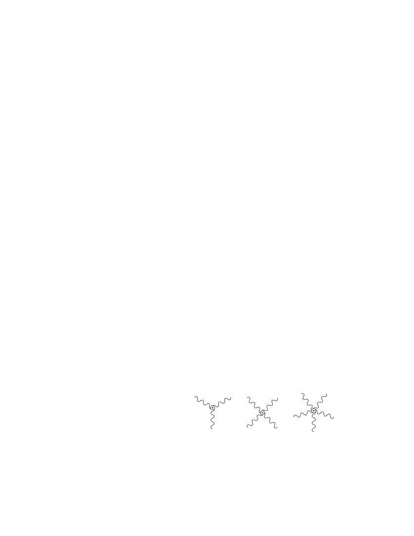
Figure 1: $\theta$-vertices

The noncommutative couplings introduce additional vertices, as depicted in Figure 1. For simplicity, we do not distinguish the gauge fields ${\cal A}_{\mu}$, $B_{\mu}^{i}$ and $G_{\mu}^{a}$ by different types of lines: the dependence on the fields is not difficult to trace.

The term $S^{\theta}_{1}$ in (2.30) is one-loop renormalizable to linear order in $\theta$ [12] since the one-loop correction to the $S^{\theta}_{1}$ is of the second order in $\theta$. We need to investigate only the renormalizability of remaining $S^{\theta}_{2}$ and $S^{\theta}_{3}$ parts of the action (2.30).

3 One-loop renormalizability

3.1 Effective action

We compute the divergencies in the one-loop effective action using the background-field method [19, 20]. As we have already explained many details of similar calculations [10], here we just introduce the notation. Let the classical action be given by $S_{cl}[\phi]$; in our case, the fields are, $\phi_{A}=({\cal A}_{\mu},\,B_{\mu}^{i},\,G_{\mu}^{a}\,)$. To quantize, one performs the functional integral. The integral over the quantum fields, ${\bf\Phi}_{A}$, can be calculated in the saddle-point approximation around the classical (background) configuration, denoted also by $\phi_{A}$. The effective action is

$$\Gamma[\phi]=S_{cl}[\phi]+\Gamma^{(1)}[\phi].$$ (3.31)

The first quantum correction to the one-loop effective action $\Gamma^{(1)}[\phi]$, is given by

$$\Gamma^{(1)}[\phi]=\frac{i}{2}\log\det S^{(2)}_{cl}[\phi]=\frac{i}{2}{\rm Tr}\,\log S^{(2)}_{cl}[\phi].$$ (3.32)

In (3.32) the $S^{(2)}_{cl}[\phi]$ is the second functional derivative of the classical action,

$$S^{(2)}_{cl}[\phi]=\frac{\delta^{2}S_{cl}}{\delta\phi_{A}\delta\phi_{B}}.$$ (3.33)

In the case of the polynomial interactions as we have in (2.30), one can find $S^{(2)}_{cl}$ simply by splitting the fields into the classical-background plus the quantum-fluctuation parts, that is, $\phi_{A}\to\phi_{A}+{\bf\Phi}_{A}$, and by computing the terms quadratic in the quantum fields. For the action (2.12), the classical Lagrangian reads

$${\cal L}_{cl} = {\cal L}_{SM}+\sum{\cal L}^{\theta}_{i}$$ (3.34)

$$= -\frac{1}{4}f_{\mu\nu}f^{\mu\nu}-\frac{1}{4}B_{\mu\nu}^{i}B^{\mu\nu i}-\frac{1}{4}G_{\mu\nu}^{a}G^{\mu\nu a}$$

$$+ g^{\prime 3}\kappa_{1}\theta^{\mu\nu}\left(\frac{a}{4}f_{\mu\nu}f_{\rho\sigma}f^{\rho\sigma}-f_{\mu\rho}f_{\nu\sigma}f^{\rho\sigma}\right)$$

$$+ g^{\prime}g^{2}\kappa_{2}\theta^{\mu\nu}\left(\frac{a}{4}f_{\mu\nu}B_{\rho\sigma}^{i}B^{\rho\sigma i}-f_{\mu\rho}B_{\nu\sigma}^{i}B^{\rho\sigma i}+c.p.\right)$$

$$+ g^{\prime}g_{S}^{2}\kappa_{3}\theta^{\mu\nu}\left(\frac{a}{4}f_{\mu\nu}G_{\rho\sigma}^{a}G^{\rho\sigma a}-f_{\mu\rho}G_{\nu\sigma}^{a}G^{\rho\sigma a}+c.p.\right).$$

Writing the $c.p.$ terms in (3.34) explicitly, we obtain

$${\cal L}_{cl} = -\frac{1}{4}f_{\mu\nu}f^{\mu\nu}-\frac{1}{4}B_{\mu\nu}^{i}B^{\mu\nu i}-\frac{1}{4}G_{\mu\nu}^{a}G^{\mu\nu a}$$

$$+ g^{\prime 3}\kappa_{1}\theta^{\mu\nu}\left(\frac{a}{4}f_{\mu\nu}f_{\rho\sigma}f^{\rho\sigma}-f_{\mu\rho}f_{\nu\sigma}f^{\rho\sigma}\right)$$

$$+ g^{\prime}g^{2}\kappa_{2}\theta^{\mu\nu}\big{(}\frac{a}{4}f_{\mu\nu}B_{\rho\sigma}^{i}B^{\rho\sigma i}-2f_{\mu\rho}B_{\nu\sigma}^{i}B^{\rho\sigma i}+\frac{a}{2}f_{\rho\sigma}B_{\mu\nu}^{i}B^{\rho\sigma i}-f_{\rho\sigma}B_{\mu\rho}^{i}B^{\nu\sigma i}\big{)}$$

$$+ g^{\prime}g^{2}_{S}\kappa_{3}\theta^{\mu\nu}\big{(}\frac{a}{4}f_{\mu\nu}G_{\rho\sigma}^{a}G^{\rho\sigma a}-2f_{\mu\rho}G_{\nu\sigma}^{a}G^{\rho\sigma a}+\frac{a}{2}f_{\rho\sigma}G_{\mu\nu}^{a}G^{\rho\sigma a}-f_{\rho\sigma}G_{\mu\rho}^{a}G^{\nu\sigma a}\big{)}\,,$$

the classical Lagrangian which we are using next in the renormalization procedure.

3.2 Interaction vertices

In order to fix the quantum gauge symmetry, we have to add the gauge-fixing term to the Lagrangian (3.1). The gauge-fixing term is added to the $\theta$-independent part in the usual way, [20, 10]. After making the splitting

$${\cal A}_{\mu}\to{\cal A}_{\mu}+{\bf A}_{\mu},\ \ B_{\mu}^{i}\to B_{\mu}^{i}+{\bf B}^{i}_{\mu},\ \ G_{\mu}^{a}\to G_{\mu}^{a}+{\bf G}^{a}_{\mu},$$ (3.36)

we obtain for the quadratic part of the action (3.1):

$$\frac{1}{2}\left(\matrix{{\bf A}_{\alpha}\,{\bf B}_{\alpha}^{i}\,{\bf G}_{\alpha}^{a}}\right)\left(\matrix{&g^{\alpha\beta}\Box+M^{\alpha\beta}&*&*\cr&*&g^{\alpha\beta}\delta^{ij}\Box+V^{\alpha\beta;ij}&0\cr&*&0&g^{\alpha\beta}\delta^{ab}\Box+W^{\alpha\beta ab}\cr}\right)\left(\matrix{{\bf A}_{\beta}\cr{\bf B}_{\beta}^{j}\cr{\bf G}_{\beta}^{b}}\right).$$ (3.37)

In (3.37), $*$ stands for the terms which will not contribute to linear order: they give higher-order corrections. The first matrix element in (3.37) is given by $M^{\alpha\beta}=\overleftarrow{\partial_{\mu}}M^{\mu\alpha,\nu\beta}(x)\overrightarrow{\partial_{\nu}}$, where

$$M^{\mu\rho,\nu\sigma} = {1\over 2}\,(g^{\mu\nu}g^{\rho\sigma}-g^{\mu\sigma}g^{\nu\rho})\theta^{\alpha\beta}f_{\alpha\beta}$$ (3.38)

$$+ g^{\mu\nu}(\theta^{\alpha\rho}{f^{\sigma}}_{\alpha}+\theta^{\alpha\sigma}{f^{\rho}}_{\alpha})+g^{\rho\sigma}(\theta^{\alpha\mu}{f^{\nu}}_{\alpha}+\theta^{\alpha\nu}{f^{\mu}}_{\alpha})$$

$$- g^{\mu\sigma}(\theta^{\alpha\rho}{f^{\nu}}_{\alpha}+\theta^{\alpha\nu}{f^{\rho}}_{\alpha})-g^{\nu\rho}(\theta^{\alpha\sigma}{f^{\mu}}_{\alpha}+\theta^{\alpha\mu}{f^{\sigma}}_{\alpha})$$

$$+ \theta^{\mu\rho}f^{\nu\sigma}+\theta^{\nu\sigma}f^{\mu\rho}-\theta^{\rho\sigma}f^{\mu\nu}-\theta^{\mu\nu}f^{\rho\sigma}-\theta^{\nu\rho}f^{\mu\sigma}-\theta^{\mu\sigma}f^{\nu\rho}\ .$$

The structure of $V^{\alpha\beta;ij}$ is as follows:

$$V^{\alpha\beta;ij}=(N_{1}+N_{2}+T_{1}+T_{2}+T_{3})^{\alpha\beta;ij}.$$ (3.39)

The operators $N_{1}$ and $N_{2}$ come from the commutative 3-vertex and 4-vertex interactions:

$$(N_{1})^{ij}_{\alpha\beta} = -2ig_{\alpha\beta}(B_{\mu})^{ij}\partial^{\mu}-i(\partial^{\mu}B_{\mu})^{ij}g_{\alpha\beta},$$ (3.40)

$$(N_{2})^{ij}_{\alpha\beta} = -(B_{\mu}B^{\mu})^{ij}g_{\alpha\beta}-2i(B_{\alpha\beta})^{ij}\,,$$ (3.41)

where we have used the notation $(X_{\mu})^{ij}=-if^{ijk}X^{k}_{\mu}$. The operators $T_{1}$, $T_{2}$ and $T_{3}$ describe the $\theta$-linear, that is the noncommutative vertices. They are more involved:

$$(T_{1})_{\alpha\beta}^{ij} = g^{\prime}g^{2}\kappa_{2}\delta^{ij}\Big{[}a(\overleftarrow{\partial_{\mu}}\theta^{\rho\sigma}f_{\rho\sigma}g_{\alpha\beta}\overrightarrow{\partial_{\mu}}-\overleftarrow{\partial_{\beta}}\theta^{\rho\sigma}f_{\rho\sigma}\overrightarrow{\partial_{\alpha}})$$

$$- 2(\overleftarrow{\partial_{\beta}}\theta_{\rho\alpha}f^{\mu\rho}\overrightarrow{\partial_{\mu}}-\overleftarrow{\partial^{\nu}}\theta^{\rho}_{\ \alpha}f_{\beta\rho}\overrightarrow{\partial_{\nu}}-\overleftarrow{\partial_{\sigma}}\theta^{\rho\sigma}f_{\mu\rho}g_{\alpha\beta}\overrightarrow{\partial^{\mu}}+\overleftarrow{\partial_{\sigma}}\theta^{\rho\sigma}f_{\beta\rho}\overrightarrow{\partial_{\alpha}}$$

$$+ \overleftarrow{\partial_{\mu}}\theta_{\rho\beta}f^{\mu\rho}\overrightarrow{\partial_{\alpha}}-\overleftarrow{\partial^{\nu}}\theta^{\rho}_{\ \beta}f_{\alpha\rho}\overrightarrow{\partial_{\nu}}-\overleftarrow{\partial^{\mu}}\theta^{\rho\sigma}f_{\mu\rho}g_{\alpha\beta}\overrightarrow{\partial_{\sigma}}$$

$$+ \overleftarrow{\partial_{\beta}}\theta^{\rho\sigma}f_{\alpha\rho}\overrightarrow{\partial_{\sigma}})+2a(\overleftarrow{\partial_{\rho}}\theta^{\rho}_{\ \alpha}f_{\mu\beta}\overrightarrow{\partial^{\mu}}+\overleftarrow{\partial^{\mu}}\theta^{\rho}_{\ \beta}f_{\mu\alpha}\overrightarrow{\partial_{\rho}})$$

$$- 2(\overleftarrow{\partial_{\mu}}\theta_{\alpha\beta}f^{\mu\nu}\overrightarrow{\partial_{\nu}}-\overleftarrow{\partial^{\mu}}\theta_{\alpha\sigma}f_{\mu\beta}\overrightarrow{\partial^{\sigma}}-\overleftarrow{\partial^{\sigma}}\theta_{\beta\sigma}f_{\mu\alpha}\overrightarrow{\partial^{\mu}}+\overleftarrow{\partial_{\rho}}\theta^{\rho\sigma}f_{\alpha\beta}\overrightarrow{\partial_{\sigma}})\Big{]},$$

$$(T_{2})^{ij}_{\alpha\beta} = g^{\prime}g^{2}i\kappa_{2}\Big{[}a(-\overleftarrow{\partial_{\mu}}\theta^{\rho\sigma}g_{\alpha\beta}f_{\rho\sigma}(B^{\mu})^{ij}-\theta^{\rho\sigma}f_{\rho\sigma}g_{\alpha\beta}(B^{\mu})^{ji}\overrightarrow{\partial_{\mu}}$$

$$+ \overleftarrow{\partial_{\beta}}\theta^{\rho\sigma}f_{\rho\sigma}(B_{\alpha})^{ij}+\theta^{\rho\sigma}f_{\rho\sigma}(B_{\beta})^{ji}\overrightarrow{\partial_{\alpha}}+\theta_{\rho\sigma}f^{\rho\sigma}(B_{\alpha\beta})^{ij})$$

$$- 2(-\overleftarrow{\partial_{\beta}}\theta_{\rho\alpha}f^{\mu\rho}(B_{\mu})^{ij}-\theta_{\rho\beta}f^{\mu\rho}(B_{\mu})^{ji}\overrightarrow{\partial_{\alpha}}+\overleftarrow{\partial_{\nu}}\theta_{\rho\alpha}f_{\beta}^{\ \rho}(B^{\nu})^{ij}$$

$$+ \theta_{\rho\beta}f_{\alpha}^{\ \rho}(B^{\nu})^{ji}\overrightarrow{\partial_{\nu}}+\overleftarrow{\partial_{\sigma}}\theta^{\rho\sigma}f_{\mu\rho}g_{\alpha\beta}(B^{\mu})^{ij}+\theta^{\rho\sigma}f_{\mu\rho}g_{\alpha\beta}(B^{\mu})^{ji}\overrightarrow{\partial_{\sigma}}$$

$$- \overleftarrow{\partial_{\sigma}}\theta^{\rho\sigma}f_{\beta\rho}(B_{\alpha})^{ij}-\theta^{\rho\sigma}f_{\alpha\rho}(B_{\beta})^{ji}\overrightarrow{\partial_{\sigma}}-\overleftarrow{\partial_{\mu}}\theta_{\rho\beta}f^{\mu\rho}(B_{\alpha})^{ij}-\theta_{\rho\alpha}f^{\mu\rho}(B_{\beta})^{ji}\overrightarrow{\partial_{\mu}}$$

$$+ \overleftarrow{\partial_{\mu}}\theta^{\rho\sigma}g_{\alpha\beta}f^{\mu}_{\ \rho}(B_{\sigma})^{ij}+\theta^{\rho\sigma}f_{\mu\rho}g_{\alpha\beta}(B_{\sigma})^{ji}\overrightarrow{\partial^{\mu}}+\overleftarrow{\partial_{\mu}}\theta^{\rho}_{\ \beta}f_{\alpha\rho}(B^{\mu})^{ij}$$

$$+ \theta_{\rho\alpha}f_{\beta}^{\ \rho}(B^{\mu})^{ji}\overrightarrow{\partial_{\mu}}-\overleftarrow{\partial_{\beta}}\theta^{\rho\sigma}f_{\alpha\rho}(B_{\sigma})^{ij}-\theta^{\rho\sigma}f_{\beta\rho}(B_{\sigma})^{ji}\overrightarrow{\partial_{\alpha}}+\theta^{\rho\sigma}f_{\alpha\rho}(B_{\beta\sigma})^{ij}$$

$$+ \theta_{\rho\beta}f^{\mu\rho}(B_{\mu\alpha})^{ij}+\theta^{\rho\sigma}f_{\beta\rho}(B_{\alpha\sigma})^{ji}$$

$$+ \theta_{\rho\alpha}f^{\mu\rho}(B^{\mu}_{\ \beta})^{ji})-2a(\overleftarrow{\partial^{\rho}}\theta_{\rho\alpha}f_{\mu\beta}(B^{\mu})^{ij}+\theta_{\rho\beta}f_{\mu\alpha}(B^{\mu})^{ji}\overrightarrow{\partial^{\rho}}$$

$$+ \overleftarrow{\partial^{\mu}}\theta_{\rho\beta}f_{\mu\alpha}(B^{\rho})^{ij}+\theta_{\rho\alpha}f_{\mu\beta}(B^{\rho})^{ji}\overrightarrow{\partial^{\mu}}-\frac{1}{2}\theta_{\rho\sigma}f_{\alpha\beta}(B^{\rho\sigma})^{ij}$$

$$- \frac{1}{2}\theta_{\alpha\beta}f_{\rho\sigma}(B^{\rho\sigma})^{ij})-2(-\overleftarrow{\partial^{\mu}}\theta_{\alpha\beta}f_{\mu\nu}(B^{\nu})^{ij}-\theta_{\beta\alpha}f_{\mu\nu}(B^{\nu})^{ji}\overrightarrow{\partial^{\mu}}$$

$$+ \overleftarrow{\partial^{\mu}}\theta_{\alpha\sigma}f_{\mu\beta}(B^{\sigma})^{ij}+\theta_{\beta\sigma}f_{\mu\alpha}(B^{\sigma})^{ji}\overrightarrow{\partial^{\mu}}+\overleftarrow{\partial^{\rho}}\theta_{\rho\beta}f_{\alpha\nu}(B^{\nu})^{ij}+\theta_{\rho\alpha}f_{\beta\nu}(B^{\nu})^{ji}\overrightarrow{\partial^{\rho}}$$

$$- \overleftarrow{\partial_{\rho}}\theta_{\beta\sigma}f_{\alpha\beta}(B_{\sigma})^{ij}-\theta^{\rho\sigma}f_{\beta\alpha}(B_{\sigma})^{ji}\overrightarrow{\partial_{\rho}}+\theta_{\beta\sigma}f_{\alpha\nu}(B^{\nu\sigma})^{ij}+\theta_{\alpha\sigma}f_{\beta\nu}(B^{\nu}_{\ \sigma})^{ji})\Big{]},$$

$$(T_{3})_{\alpha\beta}^{ij} = g^{\prime}g^{2}\kappa_{2}\Big{[}a(\theta^{\rho\sigma}f_{\rho\sigma}(B_{\mu}B^{\mu})^{ij}g_{\alpha\beta}-\theta^{\rho\sigma}f_{\rho\sigma}(B_{\beta}B_{\alpha})^{ij})$$

$$- 2(\theta_{\rho\alpha}f^{\mu\rho}(B_{\beta}B_{\mu})^{ij}-\theta^{\rho}_{\ \alpha}f_{\beta\rho}(B_{\nu}B^{\nu})^{ij}-\theta^{\rho\sigma}f_{\mu\rho}(B_{\sigma}B^{\mu})^{ij}g_{\alpha\beta}$$

$$+ \theta^{\rho\sigma}f_{\beta\rho}(B_{\sigma}B_{\alpha})^{ij}+(\alpha\leftrightarrow\beta\ \ i\leftrightarrow j))$$

$$+ 2a(\theta_{\rho\alpha}f_{\mu\beta}(B^{\rho}B^{\mu})^{ij}+2\theta_{\rho\beta}f_{\mu\alpha}(B^{\rho}B^{\mu})^{ji})$$

$$- 2(\theta_{\alpha\beta}f^{\mu\nu}(B_{\mu}B_{\nu})^{ij}-\theta_{\alpha\sigma}f_{\mu\beta}(B^{\mu}B^{\sigma})^{ij}-\theta_{\beta\sigma}f_{\mu\alpha}(B^{\mu}B^{\sigma})^{ji}+\theta^{\rho\sigma}f_{\alpha\beta}(B_{\rho}B_{\sigma})^{ij})\Big{]}.$$

We do not write the matrix $W^{\alpha\beta,ab}$ explicitly as it is completely analogous to $V^{\alpha\beta,ij}$ up to the change $B_{\mu}^{i}\leftrightarrow G_{\mu}^{a}$.

3.3 Divergencies

We compute the divergencies due to the $\,\rm U(1)_{Y}-SU(2)_{L}\,$ part of the noncommutative action, $S^{\theta}_{2}$. The result for $\,\rm U(1)_{Y}-SU(3)_{C}\,$ is analogous and follows immediately. The one-loop effective action is

$$\Gamma^{(1)}_{\theta,2} = \frac{i}{2}{\rm Tr}\,\log\left({\cal I}+\Box^{-1}(N_{1}+N_{2}+T_{1}+T_{2}+T_{3})\right)$$

$$= \frac{i}{2}\,\sum_{n=1}^{\infty}\frac{(-1)^{n+1}}{n}{\rm Tr}\,\left(\Box^{-1}N_{1}+\Box^{-1}N_{2}+\Box^{-1}T_{1}+\Box^{-1}T_{2}+\Box^{-1}T_{3}\right)^{n}.$$

For dimensional reasons, the divergencies in $\theta$-linear order are all of the form $\theta fB^{2}$. Consequently, from the sum (3.3) we need to extract and compute only terms that contain three external fields. A careful analysis gives that these terms are

$$\Gamma^{(1)}_{\theta,2}=\frac{i}{2}{\rm Tr}\,[(\Box^{-1}N_{1})^{2}\Box^{-1}T_{1}-\Box^{-1}N_{1}\Box^{-1}T_{2}-\Box^{-1}N_{2}\Box^{-1}T_{1}].$$ (3.46)

As one can readily see, only the vertices obtain divergent contributions. For the $\theta$-3-vertex, the diagrams which correspond to the traces in (3.3) are given in Figure 2.

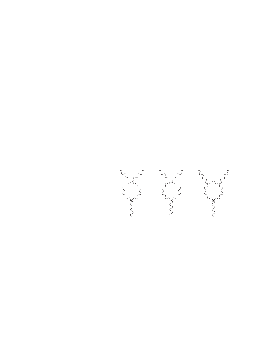
Figure 2: One-loop divergent corrections to the $\theta$-3-vertex.

Being written in terms of the field strengths, that is covariantly, (3.3) also contains the contributions to the $\theta$-4-vertex and $\theta$-5-vertex.We do not draw the corresponding diagrams: they can be easily obtained from Figure 2 by adding external legs (in accordance with the Feynman rules). The divergent part of (3.46) is calculated in the momentum representation by dimensional regularization. The results are given by

$${\rm Tr}\,(\Box^{-1}N_{1}\Box^{-1}T_{2}) = \frac{4i}{3(4\pi)^{2}\epsilon}g^{\prime}g^{2}\kappa_{2}$$ (3.47)

$$\times \Big{[}(6-2a)(\theta^{\rho\sigma}f_{\alpha\rho}+\theta_{\rho\alpha}f^{\sigma\rho})(B^{\alpha i}\partial_{\mu}\partial_{\sigma}B^{\mu i}-B^{\alpha i}\Box B^{i}_{\sigma})$$

$$+ (3a-4)\theta^{\rho\sigma}f_{\rho\sigma}(B^{\nu i}\partial_{\mu}\partial_{\nu}B^{\mu i}-B_{\mu}^{i}\Box B^{\mu i})\Big{]},$$

$${\rm Tr}\,(\Box^{-1}N_{2}\Box^{-1}T_{1}) = \frac{4i}{3(4\pi)^{2}\epsilon}g^{\prime}g^{2}\kappa_{2}$$ (3.48)

$$\times \Big{[}(2a-6)(\theta^{\rho\sigma}f_{\alpha\rho}+\theta_{\rho\alpha}f^{\sigma\rho})(B^{\nu i}\partial_{\sigma}\partial^{\alpha}B_{\nu}^{i}+\partial_{\sigma}B^{\mu i}\partial^{\alpha}B_{\mu}^{i})$$

$$+ \theta^{\rho\sigma}f_{\rho\sigma}(18-11a)(\partial_{\nu}B^{\nu i}\partial_{\mu}B^{\mu i}+B_{\mu}^{i}\Box B^{\mu i})\Big{]},$$

$${\rm Tr}\,(\Box^{-1}N_{1}^{2}\Box^{-1}T_{1}) = \frac{4i}{3(4\pi)^{2}\epsilon}g^{\prime}g^{2}\kappa_{2}\Big{[}\theta^{\rho\sigma}f_{\rho\sigma}\Big{(}(22-14a)B_{\mu}^{i}\Box B^{\mu i}$$ (3.49)

$$+ (15-10a)\partial_{\nu}B^{\mu i}\partial^{\nu}B_{\mu}^{i}$$

$$+ (3a-4)B^{\mu i}\partial_{\mu}\partial_{\nu}B^{\nu i}+(3-a)\partial_{\mu}B^{\nu i}\partial_{\nu}B^{\mu i}\Big{)}$$

$$+ (\theta^{\rho\sigma}f_{\alpha\rho}+\theta_{\rho\alpha}f^{\sigma\rho})\Big{(}(2a-6)(B_{\sigma}^{i}\Box B^{\alpha i}$$

$$- B_{\sigma}^{i}\partial^{\alpha}\partial_{\mu}B^{\mu i}+B^{\mu i}\partial_{\sigma}\partial^{\alpha}B_{\mu}^{i}-\partial_{\sigma}B^{\mu i}\partial_{\mu}B^{\alpha i})+(a-3)\partial_{\mu}B^{\alpha i}\partial^{\mu}B_{\sigma}^{i}$$

$$+ (3a-9)\partial_{\sigma}B^{\mu i}\partial^{\alpha}B_{\mu}^{i}\Big{)}\Big{]}.$$

Their sum, that is the complete divergent part due to the $\,\rm U(1)_{Y}-SU(2)_{L}\,$ gauge boson interaction is

$$\Gamma^{(1)}=\frac{4}{3(4\pi)^{2}\epsilon}g^{\prime}g^{2}\kappa_{2}(3-a)\theta^{\mu\nu}\int d^{4}x\,\big{(}\frac{1}{4}f_{\mu\nu}B_{\rho\sigma}^{i}B^{\rho\sigma i}-f_{\mu\rho}B_{\nu\sigma}^{i}B^{\rho\sigma i}\big{)}.$$ (3.50)

Adding to this expression the divergencies which come from the commutative part ofthe action, and also those induced by the $\,\rm U(1)_{Y}-SU(3)_{C}\,$ mixing, we obtain the full result for the divergent one-loop effective action linear in $\theta$:

$$\Gamma_{div} = \frac{11}{3(4\pi)^{2}\epsilon}\int d^{4}xB_{\mu\nu}^{i}B^{\mu\nu i}+\frac{11}{2(4\pi)^{2}\epsilon}\int d^{4}xG_{\mu\nu}^{a}G^{\mu\nu a}$$ (3.51)

$$+ \frac{4}{3(4\pi)^{2}\epsilon}g^{\prime}g^{2}\kappa_{2}(3-a)\theta^{\mu\nu}\int d^{4}x\big{(}\frac{1}{4}f_{\mu\nu}B_{\rho\sigma}^{i}B^{\rho\sigma i}-f_{\mu\rho}B_{\nu\sigma}^{i}B^{\rho\sigma i}\big{)}$$

$$+ \frac{6}{3(4\pi)^{2}\epsilon}g^{\prime}g^{2}_{S}\kappa_{3}(3-a)\theta^{\mu\nu}\int d^{4}x\big{(}\frac{1}{4}f_{\mu\nu}G_{\rho\sigma}^{a}G^{\rho\sigma a}-f_{\mu\rho}G_{\nu\sigma}^{a}G^{\rho\sigma a}\big{)}.$$

The divergent contribution due to $\rm U(1)_{Y}$ solely vanishes, both the commutative and the noncommutative one.

3.4 Counterterms

It is clear from (3.51) that the divergencies in the noncommutative sector vanish for the choice $a=3$. Therefore one obtains that the noncommutative gauge sector interaction is not only renormalizable but finite. The renormalization is performed by adding counterterms to the Lagrangian. We obtain

$${\cal L}+{\cal L}_{ct} = -\frac{1}{4}{f_{0}}_{\mu\nu}{f_{0}}^{\mu\nu}-\frac{1}{4}{B_{0}}_{\mu\nu}^{i}{B_{0}}^{\mu\nu i}-\frac{1}{4}{G_{0}}_{\mu\nu}^{a}{G_{0}}^{\mu\nu a}$$ (3.52)

$$+ g^{\prime 3}\kappa_{1}\theta^{\mu\nu}\left(\frac{3}{4}{f_{0}}_{\mu\nu}{f_{0}}_{\rho\sigma}{f_{0}}^{\rho\sigma}-{f_{0}}_{\mu\rho}{f_{0}}_{\nu\sigma}{f_{0}}^{\rho\sigma}\right)$$

$$+ g_{0}^{\prime}g_{0}^{2}\kappa_{2}\theta^{\mu\nu}\left(\frac{3}{4}{f_{0}}_{\mu\nu}{B_{0}}_{\rho\sigma}^{i}B_{0}^{\rho\sigma i}-{f_{0}}_{\mu\rho}{B_{0}}_{\nu\sigma}^{i}B_{0}^{\rho\sigma i}+c.p.\right)$$

$$+ g_{0}^{\prime}(g_{S})_{0}^{2}\kappa_{3}\theta^{\mu\nu}\left(\frac{3}{4}{f_{0}}_{\mu\nu}{G_{0}}_{\rho\sigma}^{a}G_{0}^{\rho\sigma a}-{f_{0}}_{\mu\rho}{G_{0}}_{\nu\sigma}^{a}G_{0}^{\rho\sigma a}+c.p.\right),$$

where the bare quantities are given as follows:

$${{\cal A}_{0}}^{\mu} = {\cal A}^{\mu}\,,\qquad g_{0}^{\prime}=g^{\prime}\,,$$ (3.53)

$${B_{0}}^{\mu i} = B^{\mu i}\sqrt{1+\frac{44g^{2}}{3(4\pi)^{2}\epsilon}}\,,\quad g_{0}=\frac{g\,\mu^{\epsilon/2}}{\sqrt{1+\frac{44g^{2}}{3(4\pi)^{2}\epsilon}}}\,,$$ (3.54)

$${G_{0}}^{\mu a} = G^{\mu a}\sqrt{1+\frac{22g_{S}^{2}}{(4\pi)^{2}\epsilon}}\,,\quad{(g_{S})}_{0}=\frac{g_{S}\,\mu^{\epsilon/2}}{\sqrt{1+\frac{22g_{S}^{2}}{(4\pi)^{2}\epsilon}}}\,.$$ (3.55)

In order to keep the constants $\kappa_{1}$, $\kappa_{2}$ and $\kappa_{3}$ in (3.52) unchanged under the renormalization procedure, i.e.

$$\kappa_{1}=\,{(\kappa_{1})}_{0}\,,\>\>\;\kappa_{2}=\,{(\kappa_{2})}_{0}\,,\>\>\;\kappa_{3}=\,{(\kappa_{3})}_{0}\,,$$ (3.56)

we obtain the following renormalization of the constants $C({\cal R})$

$$C_{1} = {(C_{1})}_{0}+\frac{33}{18(4\pi)^{2}\epsilon}\,,\quad C_{2}={(C_{2})}_{0}-\frac{11}{18(4\pi)^{2}\epsilon}\,,\quad C_{3}={(C_{3})}_{0}-\frac{11}{18(4\pi)^{2}\epsilon}\,,$$

$$C_{4} = {(C_{4})}_{0}-\frac{143}{18(4\pi)^{2}\epsilon}\,,\quad C_{5}={(C_{5})}_{0}-\frac{121}{18(4\pi)^{2}\epsilon}\,,\quad C_{6}={(C_{6})}_{0}+\frac{110}{18(4\pi)^{2}\epsilon}\,.$$

Finally, an important point is that the noncommutativity parameter $\theta$ need not be renormalized.

4 Discussion and conclusion

We have constructed a version of the standard model on the noncommutative Minkowski space which is one-loop renormalizable and finite in the gauge sector and in first order in the $\theta$ parameter. The renormalizability in the model was obtained by choosing six particle representations of the matter fields for the first generation of the SM as in Table 1, and by fixing the arbitrariness in the $\theta$-linear expansion terms in the Seiberg-Witten map.

The one-loop renormalizability of the NCSM gauge sector is certainly a very encouraging result from both theoretical and experimental perspectives. So far, this property has not concerned fermions: the results on the renormalizability of noncommutative theories including the Dirac fermions are negative, [9, 10]. However, the present result could be an indication that the inclusion of fermions in a renormalizable theory might be possible by a more careful choice of representation as well.

Our result also has an important consequence on the phenomenological analysis of the $1\to 2$ [6, 13, 17] and $2\to 2$ [14, 15, 16] processes in elementary particle physics. Namely, in the gauge sector of the noncommutative standard model the above transitions contain triple gauge boson interactions induced by noncommutativity and, according to (3.51), they can be safely used further on. Since the triple gauge boson couplings have already been used in a number of phenomenological predictions to determine of the scale of noncommutativity [6, 7, 13, 17], the regular behaviour of these TGB interactions with respect to the one-loop renormalizability puts all of our predictions from the NCSM gauge sector to a much firmer ground.

Experimentally, there are chances to detect, in the forthcoming experiments at LHC, the decays forbidden in the SM but kinematically allowed, like $Z\to\gamma\gamma$, and/or to find deviations of ${\bar{f}}f\to\gamma\gamma$, etc. scatterings with respect to the standard model predictions. Finally, the discovery of forbidden decays, and/or measurements of differential cross section distributions deviating from the SM predictions, would certainly prove a violation of the SM as we know it at present and could serve as a possible indication/signal for space-time noncommutativity.

References

• [1] M. Kontsevich, Deformation quantization of Poisson manifolds, I, Lett. Math. Phys.  66 (2003) 157 [q-alg/9709040].
• [2] N. Seiberg and E. Witten, String theory and noncommutative geometry, JHEP 09 (1999) 032 [hep-th/9908142].
• [3] J. Madore, S. Schraml, P. Schupp and J. Wess, Gauge theory on noncommutative spaces, Eur. Phys. J. C16 (2000) 161 [hep-th/0001203]; B. Jurčo, S. Schraml, P. Schupp and J. Wess, Enveloping algebra valued gauge transformations for non-Abelian gauge groups on non-commutative spaces, Eur. Phys. J. C17 (2000) 521 [hep-th/0006246]; B. Jurčo, L. Möller, S. Schraml, P. Schupp and J. Wess, Construction of non-Abelian gauge theories on noncommutative spaces, Eur. Phys. J. C21 (2001) 383 [hep-th/0104153].
• [4] X. Calmet, B. Jurčo, P. Schupp, J. Wess and M. Wohlgenannt, The standard model on non-commutative space-time, Eur. Phys. J. C23 (2002) 363 [hep-ph/0111115].
• [5] P. Aschieri, B. Jurčo, P. Schupp and J. Wess, Non-Commutative GUTs, Standard Model and C,P,T, Nucl. Phys. B651 (2003) 45 [hep-th/0205214].
• [6] W. Behr, N.G. Deshpande, G.  Duplančić, P. Schupp, J. Trampetić and J. Wess, The Z $\to\,\,\gamma\gamma,gg$ Decays in the Noncommutative Standard Model,Eur. Phys. J. C29 (2003) 441 [hep-ph/0202121]; G. Duplančić, P. Schupp and J. Trampetić, Comment on triple gauge boson interactions in the non-commutative electroweak sector, Eur. Phys. J. C32 (2003) 141 [hep-ph/0309138].
• [7] B. Melic, K. Passek-Kumericki, J. Trampetic, P. Schupp and M. Wohlgenannt, The standard model on non-commutative space-time: Electroweak currents and Higgs sector, Eur. Phys. J. C 42 (2005) 483 [arXiv:hep-ph/0502249]. B. Melic, K. Passek-Kumericki, J. Trampetic, P. Schupp and M. Wohlgenannt, The standard model on non-commutative space-time: Strong interactions included, Eur. Phys. J. C 42 (2005) 499 [arXiv:hep-ph/0503064].
• [8] F. Brandt, C.P. Martin and F. Ruiz Ruiz, Anomaly freedom in Seiberg-Witten noncommutative gauge theories, JHEP 07 (2003) 068 [hep-th/0307292].
• [9] R. Wulkenhaar, Non-Renormalizability Of Theta-Expanded Noncommutative QED, JHEP 0203 (2002) 024 [arXiv:hep-th/0112248].
• [10] M. Buric and V. Radovanovic, The one-loop effective action for quantum electrodynamics on noncommutative space, JHEP 0210 (2002) 074 [arXiv:hep-th/0208204]; M. Buric and V. Radovanovic, Non-renormalizability of noncommutative SU(2) gauge theory, JHEP 0402 (2004) 040 [arXiv:hep-th/0401103]; M. Buric and V. Radovanovic, On Divergent 3-Vertices In Noncommutative SU(2) Gauge Theory, Class. Quant. Grav.  22 (2005) 525 [arXiv:hep-th/0410085].
• [11] A. Bichl, J. Grimstrup, H. Grosse, L. Popp, M. Schweda and R. Wulkenhaar, Renormalization of the noncommutative photon self-energy to all orders via Seiberg-Witten map, JHEP 06 (2001) 013 [hep-th/0104097].
• [12] M. Buric, D. Latas and V. Radovanovic, Renormalizability of noncommutative SU(N) gauge theory, JHEP 0602 (2006) 046 [arXiv:hep-th/0510133].
• [13] J. Trampetić, Rare and forbidden decays, Acta Phys. Polon. B33 (2002) 4317 [hep-ph/0212309]; B. Melic, K. Passek-Kumericki and J. Trampetic, Quarkonia decays into two photons induced by the space-time non-commutativity, Phys. Rev. D 72 (2005) 054004 [arXiv:hep-ph/0503133]. B. Melic, K. Passek-Kumericki and J. Trampetic, K $\to$ pi gamma decay and space-time noncommutativity, Phys. Rev. D 72 (2005) 057502 [arXiv:hep-ph/0507231].
• [14] J. L. Hewett, F. J. Petriello and T. G. Rizzo, Signals for non-commutative interactions at linear colliders, Phys. Rev. D 64 (2001) 075012 [hep-ph/0010354];
• [15] T. Ohl and J. Reuter, Testing the noncommutative standard model at a future photon collider, Phys. Rev. D70 (2004) 076007 [hep-ph/0406098]; A. Alboteanu, T. Ohl and R. Ruckl, Collider tests of the non-commutative standard model, PoS HEP2005 (2006) 322 [arXiv:hep-ph/0511188].
• [16] G. Abbiendi et al. [OPAL Collaboration], Test of non-commutative QED in the process e+ e- $\to$ gamma gamma at LEP, Phys. Lett. B 568, 181 (2003) [hep-ex/0303035].
• [17] P. Schupp, J. Trampetić, J. Wess and G. Raffelt, The photon neutrino interaction in non-commutative gauge field theory and astrophysical bounds, Eur. Phys. J. C 36 (2004) 405 [hep-ph/0212292]. P. Minkowski, P. Schupp and J. Trampetić, Neutrino dipole moments and charge radii in non-commutative space-time, Eur. Phys. J. C 37 (2004) 123 [hep-th/0302175].
• [18] T. Asakawa and I. Kishimoto, Comments On Gauge Equivalence In Noncommutative Geometry, JHEP 9911 (1999) 024 [arXiv:hep-th/9909139].
• [19] G. ’t Hooft, An algorithm for the poles at dimension four in the dimensional regularization procedure, Nucl. Phys. B 62 (1973) 444.
• [20] M. E. Peskin and D. V. Schroeder, An introduction to Field Theory, Perseus Books, Reading 1995.