Gluino zero-modes for non-trivial holonomy calorons

Abstract:

We couple fermion fields in the adjoint representation (gluinos) to the SU(2) gauge field of unit charge calorons defined on $R^{3}\times S_{1}$. We compute corresponding zero-modes of the Dirac equation. These are relevant in semiclassical studies of ${\cal N}=1$ Super-symmetric Yang-Mills theory. Our formulas, show that, up to a term proportional to the vector potential, the modes can be constructed by different linear combinations of two contributions adding up to the total caloron field strength.

1 Introduction

In recent years a deep link between monopoles and instantons has been established at finite temperature [1]-[5]. It was for long known that the finite temperature instanton, the Harrington-Shepard caloron [6], becomes for large scale parameter a BPS monopole [7]. This happens when the value of the constant Polyakov loop at infinity, the holonomy, approaches unity. The surprise came with the discovery that non-trivial holonomy calorons when squeezed in the time direction reveal to be composed of $N$, for $SU(N)$, BPS monopoles. $N-1$ of these constituent monopoles are massless for the HS caloron, but in general all of them get non-zero masses with values related to the eigenvalues of the Polyakov loop at infinity. The idea of the composite nature of instantons, with instanton quarks [8] or merons [9] as constituents, has been on the basis of several semiclassical proposals to address the confinement problem in QCD. Isolated fractional instantons (twisted instantons)[10] can be obtained by using tori with twisted boundary conditions [11]. By replicating the tori one can obtain classical configurations in a periodic box, where the action density is clustered into lumps of $1/N$ of topological charge. These structures were observed in lattice generated ensembles at zero temperature and were argued to be relevant for QCD confinement [12]. Non-trivial holonomy calorons also exhibit explicitly this composite nature as far as the separation between constituents stays larger that their size. Otherwise they merge in an undissociated instanton. Triggered by this result, quite a number of more recent lattice analysis have identified the presence of constituent monopoles at temperatures below but close to the deconfinement phase transition in Monte-Carlo generated configurations [13, 14]. The possible relevance of the instanton-monopole link for QCD dynamics is an open issue, nevertheless constituent monopoles have already shown their usefulness in a different context, in particular for calculations of the gluino condensate in 4D ${\cal N}=1$ supersymmetric Yang-Mills theory [15]. The contribution of the constituent monopoles seems essential there to bring to agreement strong and weak-coupling instanton calculations of the condensate.

The existence of an analytic expression for the non-trivial holonomy calorons allowed a subsequent analytic calculation of the zero-modes of the Dirac equation, in the fundamental representation, in this background field[16, 17]. For large constituent separation the modes are entirely supported on just one of the monopoles, jumping from one to other as we change the periodicity condition in the time-like direction imposed on the solution. This knowledge has proven useful in interpreting the results of several lattice studies which employ low-lying eigenstates of the Dirac operator to trace topological structures present in gauge field configuration ensembles [13], [18]-[20].

The present paper is devoted to the derivation of the analytic expression and properties of the zero-modes of the Dirac equation in the adjoint representation for Q=1 SU(2) calorons. These are relevant objects in the study of the semiclassical behaviour of 4D ${\cal N}=1$ supersymmetric Yang-Mills theory compactified in $R^{3}\times S^{1}$. They are directly related to estimates of the gluino-condensate [21]. By now this has been studied [15] only in the limit of large constituent separation, in which the SU(2) caloron degenerates into two BPS monopoles. Our expressions for the four adjoint modes, valid for any separation, indeed tend in this limit to two pairs, one attached to each constituent monopole reproducing the well known adjoint zero modes of BPS monopoles [7].

Our work is also useful within the previously mentioned spirit of using modes of the Dirac equation as probes of gauge field structure, an approach that has become very popular (see for instance [22]- [25]) since the discovery of lattice Dirac operators [26] that possess exact index theorems. The usefulness of adjoint modes in this respect has been recently advocated [27]. The idea is based upon the so called supersymmetric modes, having densities that match the action density profile but are less sensitive to ultraviolet fluctuations.

The paper is organised as follows. In section 2 we describe the general properties of adjoint zero-modes, such as their occurrence in pairs, related by Euclidean CP transformations. Then, we give the main formula for the modes within the ADHM formulation, and apply it to the $Q=1$ SU(2) caloron case. This provides two pairs of zero-modes. One pair is given by the supersymmetric zero modes, which are proportional to the gauge field strength itself. The remaining pair of adjoint zero modes is studied. In addition to the analytical expression (details of its derivation are given in the Appendix), we display its density profile in some representative cases. In section 3 we show how the solutions behave in certain limits and how they interpolate between modes of BPS monopoles and those of instantons. We end up with a summary of the results and a list of possible extensions and applications.

2 Formalism

The adjoint zero modes $\Psi^{a}_{\alpha}(x)$ are solutions of the Euclidean 4-dimensional massless covariant Dirac equation in the adjoint representation of the gauge group:

$$\not\!\!D\Psi=0$$ (1)

In this paper we will analyse the simplest case given by group SU(2). Then the colour index $a$ takes the values $1,2,3$, while the spinorial index $\alpha$ takes four values. Action by $\gamma_{5}$ maps zero-modes into other ones. It is convenient then to combine zero modes into eigenstates of $\gamma_{5}$ with eigenvalue $\pm 1$, known as left and right-handed modes respectively. In Weyl’s representation of the Dirac matrices, the left and right handed modes reduce to two-component spinors $\psi_{\pm}$ satisfying

$$\hat{D}\psi_{-} = 0$$ (2)

$$\bar{D}\psi_{+} = 0$$ (3)

where $\hat{D}=\sigma_{\mu}D_{\mu}$ and $\bar{D}=\overline{\sigma}_{\mu}D_{\mu}$. The Weyl matrices are given by $\sigma_{\mu}=(\mathbf{I},-i\vec{\tau})$, in terms of the Pauli matrices $\tau_{i}$ (the matrix $\overline{\sigma}_{\mu}$ is the hermitian conjugate of $\sigma_{\mu}$). If the gauge field is self-dual, then Eq. 2 implies

$$D_{\mu}\psi_{-}=0$$ (4)

for all $\mu$. This can easily be shown to imply that the gauge-invariant density $|\psi_{-}(x)|^{2}$ must be constant (x-independent). For non-compact space-times these are non-normalizable solutions.

Focusing now on left-handed zero modes (solutions of Eq. 3) we point out that the space of solutions is always even-dimensional. This follows from euclidean CP invariance mapping one solution into other

$$\psi_{+}\longrightarrow\psi_{+}^{c}\equiv-i\tau_{2}\psi_{+}^{\dagger}$$ (5)

In the previous formula $\psi_{+}^{\dagger}$ stands for the complex conjugate spinor and the matrix $\tau_{2}$ acts on the 2-spinor indices. Furthermore, for self-dual gauge fields one can establish a one to one correspondence between self-dual deformations $\delta A^{a}_{\mu}$ of the gauge field and left-handed zero modes. Given a deformation, one must first transform it to the background Lorentz gauge

$$D_{\mu}\delta A_{\mu}=0$$ (6)

and then one can show that

$$\psi_{+}=\delta A_{\mu}\sigma_{\mu}V$$ (7)

is a zero mode for any constant 2-spinor $V$.

If there are isommetries of the problem which do not leave the solution invariant, the corresponding deformations are associated to specific zero-modes. In particular, the super-symmetric zero-modes arising for $\delta A_{\mu}=F_{\mu 0}$, are associated with translation symmetry. In general, the space of self-dual connections is continuous and can be parameterised in terms of a set of real parameters (moduli). Variations with respect to these moduli parameters(tangent vectors) give rise to adjoint zero-modes.

Self-dual gauge fields with topological charge $Q$ on the sphere $S_{4}$ or on $R^{4}$ (with finite action) can be constructed by an algebraic procedure known as the ADHM construction [28]. The fields are written in terms of $q$, a Q dimensional column vector of quaternions, and $\widetilde{A}$, a $Q\times Q$ matrix of quaternions satisfying certain conditions, to be specified later. In what follows, we will identify quaternions with the space of two by two matrices which are real linear combinations of the Weyl matrices $\overline{\sigma}_{\mu}$. In particular, one can form the quaternion $\hat{x}=x_{\mu}\sigma_{\mu}$ and its adjoint $\bar{x}=x_{\mu}\overline{\sigma}_{\mu}$. The self-duality condition amounts to the requirement that the matrix $R$:

$$R=q\otimes q^{\dagger}+(\widetilde{A}^{\dagger}-\bar{x})(\widetilde{A}-\hat{x})$$ (8)

is real and invertible.

The self-dual deformations are then associated with variations of the ADHM data $q$ and $\widetilde{A}$  [29]. Using the previously mentioned relation between adjoint modes and deformations, one obtains the formula for the modes in terms of variations of the parameters $\delta q$ and $\delta\widetilde{A}$:

$$\delta A_{\mu}=\frac{-i}{2}(\delta q^{\dagger}-u^{\dagger}\delta\widetilde{A})\bar{\sigma}^{\mu}\hat{\partial}\omega+\mbox{h.c.}$$ (9)

where we have introduced the x-dependent vectors of quaternions $u$ and $\omega$ defined by the relations

$$\omega=R^{-1}q$$ (10)

and

$$u=F\,(\widetilde{A}-\hat{x})\omega$$ (11)

where $F=1+u^{\dagger}u$ is a real function. The symbol $\hat{\partial}$ in Eq. 9 stands for the contraction $\partial_{\mu}\sigma_{\mu}$.

The condition that the variation $\delta A_{\mu}$ given in Eq. 9 satisfies the required covariant background gauge condition is

$${\rm Re}\left(\widetilde{A}^{\dagger}\,\delta\widetilde{A}-\delta\widetilde{A}^{\dagger}\,\widetilde{A}+q(\delta q)^{\dagger}-(\delta q)q^{\dagger}\right)=0$$ (12)

where ${\rm Re}$ stands for the real part of the quaternion. This condition will be seen to hold for our formulas. Its interpretation will also become more clear later.

Now we will proceed to particularise to the case of the Q=1 caloron. This is a self-dual configuration in $R^{3}\times S_{1}$. At infinity the time-like Polyakov loop (the holonomy) is non-trivial. This is determined by the parameter $\delta_{1}$ such that the trace of the Polyakov loop at spatial infinity tends to $\cos(2\pi\delta_{1})$.

For a given holonomy and a fixed period in time $\beta$ (which we will henceforth fix to 1), solutions depend on the following parameters: the position of the center of mass of the caloron $X_{\rm CM}$, the size parameter $\rho$ and an SU(2) colour orientation. For medium and large values of $\rho$ (compared with the time-period $\beta=1$) the action density of the solution appears as a superposition of two lumps, named constituent monopoles in Ref. [1]. The distance between the lumps approaches $\pi\rho^{2}$ and the total masses $M_{a}=4\pi m_{a}/g^{2}$ are given by the holonomy as follows:

$$m_{1}=4\pi\delta_{1}\quad;\quad m_{2}=4\pi\delta_{2}=2\pi-m_{1}$$ (13)

The shapes of these monopoles tend, as the distance is increased, to that of BPS monopoles, having a non-abelian core which is exponentially localised and an abelian powerlike fall-off at large distances.

One can construct the caloron solution by an infinite dimensional generalisation of the ADHM construction [1] (strictly speaking a Nahm [30] transform). This is the procedure that we will follow here, allowing us to extend the ADHM formulas for the adjoint modes to this case. If we regard the caloron solution as a solution in $R^{4}$ which is periodic in time, the topological charge would now become infinite. Thus, $q$ and $\widetilde{A}$ become an infinite dimensional vector and matrix respectively. The discrete index can be interpreted as the Fourier mode of a periodic function of one variable $z$ (with period 1). Thus $q(z)$ is a distribution and $\widetilde{A}$ a linear operator in this space. One can use translations, rotations and gauge transformations to bring $q(z)$ and $\widetilde{A}$ to the form  [1]:

$$q(z)=\rho(\delta(z-\delta_{1})P_{+}+\delta(z+\delta_{1})P_{-})$$ (14)

$$\widetilde{A}(z)=\frac{1}{2\pi i}\frac{d}{dz}-i\vec{X}^{1}\vec{\tau}\chi_{1}(z)-i\vec{X}^{2}\vec{\tau}\chi_{2}(z)$$ (15)

where $P_{\pm}=\frac{1\pm\tau_{3}}{2}$, $\delta(z)$ are periodic delta functions and $\chi_{a}(z)$ are characteristic functions of the intervals $I_{a}$ (taking the value 1 in the interval and zero elsewhere). The intervals $I_{1}=[-\delta_{1},\delta_{1}]$ and $I_{2}=[\delta_{1},1-\delta_{1}]$ denote complementary regions of length $m_{a}/(m_{1}+m_{2})$ within one period in $z$. Finally, the vectors $\vec{X}^{a}$ can be interpreted as denoting the spatial locations of the constituent monopoles. We have used the translation and rotation symmetry to place them along the $z$ axis and to locate their center of mass at the origin ($m_{1}\vec{X}^{1}+m_{2}\vec{X}^{2}=0$). In addition, their separation is fixed by $\rho$:

$$\vec{X}^{2}-\vec{X}^{1}=\pi\rho^{2}(0,0,1)$$ (16)

This information allows to determine $\vec{X}^{a}$ uniquely. As mentioned all $Q=1$ caloron solutions can be obtained from these formulas by applying euclidean and gauge transformations. Furthermore, one can easily restore of arbitrary time period by multiplying all length parameters by $\beta$ (and masses by $1/\beta$).

Within the Nahm transform philosophy, the quantity $\widetilde{A}$ can be identified with the covariant derivative (divided by $2\pi i$) of an abelian gauge potential $\widehat{A}_{\mu}$ over a 4-d torus which has been shrunk to a circle, whose coordinate is labelled by $z$. The remaining (spatial) coordinates have dropped as arguments, but the vector potential field still keeps the vector index. In our case only the third component is non-zero, and is given by

$$\widehat{A}_{3}=-2\pi(X^{1}_{3}\chi_{1}(z)+X^{2}_{3}\chi_{2}(z))$$ (17)

This implies that the corresponding magnetic field vanishes and the electric field is a delta function over $z=\pm\delta_{1}$.

In conclusion, to obtain the expression for the adjoint zero modes for our case, one has only to substitute the expression of the variations $\delta q$ and $\delta\widetilde{A}$ in the formula Eq. 9. The variations are associated to the parameters of which the caloron field depends. On one hand we have the coordinates of the center of mass of the constituent monopoles. This will give rise to the supersymmetric modes, which are always associated to translational symmetry. The corresponding variations can be obtained straightforwardly, giving $\delta^{(0)}q=0$ and $\delta^{(0)}\widetilde{A}=\mathbf{I}$. Substituting into the formula one obtains $\delta^{(0)}A_{0}=0$ and

$$\delta^{(0)}A_{i}=E_{i}$$ (18)

where $E_{i}$ are the components of the electric (or magnetic) field strengths of the caloron. As anticipated this is the expression of the supersymmetric mode, having density proportional to the action density of the caloron field.

The index theorem suggests that we should find 4 independent solutions ($2NQ$). As mentioned previously they come in CP-pairs. Each pair is associated to 4 real variations of the Nahm data. This is exemplified with the supersymmetric modes, for which there is a single pair associated to the 4d center of mass variations. Therefore, one must still find a new independent CP-pair. As we will see, one can obtain one such mode by varying with respect to the parameter $\rho$. Acting with the operator $\rho\frac{d}{d\rho}$ on our expressions of $q$ and $\widetilde{A}$, we obtain $\delta^{(1)}q=q$ and

$$\delta^{(1)}\widetilde{A}=-2iX_{3}^{1}\tau_{3}\chi_{1}(z)-2iX_{3}^{2}\tau_{3}\chi_{2}(z)=i\rho^{2}\tau_{3}(m_{2}\chi_{1}(z)-m_{1}\chi_{2}(z))$$ (19)

For these variations $q(\delta^{(1)}q)^{\dagger}-(\delta^{(1)}q)q^{\dagger}$ vanishes, and Eq. 12 amounts to the requirement that the Nahm-dual field $\widehat{A}_{\mu}(z)$ satisfies the covariant background gauge condition too. This follows trivially, since $\delta^{(1)}\widetilde{A}_{0}=0$. In summary, substitution of these variations into Eq. 9 provides a self-dual deformation in the covariant background Lorentz gauge. The same applies to the supersymmetric zero-mode for which $\delta^{(0)}q=0$ and $\delta^{(0)}\widetilde{A}_{0}$ is constant.

To give a simple expression of the result it is convenient to separate the contribution of $\delta q$, present only in the non-supersymmetric zero-mode case from the other one. Furthermore, we point out that the former becomes proportional to the caloron vector potential itself:

$$\frac{i}{2}q^{\dagger}\bar{\sigma}_{\mu}\hat{\partial}\omega+\mbox{\rm h. c.}=\frac{2}{F}A_{\mu}$$ (20)

To give an expression of the second term one must realize that both $u$ and $\omega$ can be written as the sum of two contributions, $u=\sum_{a}u_{a}$ and $\omega=\sum_{a}\omega_{a}$, such that each piece is proportional to the characteristic function $\chi_{a}(z)$ of each of the intervals. Finally, we can collect the formula for both sets of modes as follows

$$\delta^{(0)}A_{\mu} = E^{1}_{\mu}+E^{2}_{\mu}$$ (21)

$$\delta^{(1)}A_{\mu} = -\frac{2}{F}A_{\mu}+\rho^{2}\eta^{3\mu}_{\alpha}(m_{2}E^{1}_{\alpha}-m_{1}E^{2}_{\alpha})$$ (22)

where $\eta^{3\mu}_{\alpha}$ is ‘t Hooft symbol and we have defined

$$E^{a}_{\alpha}=\frac{i}{2}u_{a}^{\dagger}\bar{\sigma}_{\alpha}\hat{\partial}\omega_{a}+\mbox{\rm h. c.}$$ (23)

which by virtue of Eq. 21 can be regarded as the contribution of constituent monopole a to the caloron field strength. This formula is quite appealing since it suggests that the two modes are simply given by different linear combinations of the field produced by each constituent monopole. This is modified by the presence of the $\eta^{3\mu}_{\alpha}$ in the expression for the non-supersymmetric mode. Notice, however, that each mode belongs to a complex two dimensional space of modes generated by the two elements of a CP-pair. In particular, this means that one can transform the gauge variations as follows

$$\delta^{\prime}A_{\beta}=\eta^{\alpha\mu}_{\beta}\delta A_{\mu}$$ (24)

for any value of $\alpha$. Using this and allowing for a different normalisation one can recast the formula for the non-supersymmetric mode as follows:

$$\delta^{{}^{\prime}(1)}A_{\mu}=-\eta^{3\alpha}_{\mu}\frac{1}{\pi F\rho^{2}}A_{\alpha}+(m_{2}E^{1}_{\mu}-m_{1}E^{2}_{\mu})/{2\pi}$$ (25)

In the appendix we compute the expressions for the functions $u_{a}$, $\omega_{a}$ and with them we compute $E^{a}_{\alpha}$. The final expression Eq. 70 is a sum of two terms. The first one is given by the field produced by a BPS monopole, of mass $M_{a}$, located at the position of the corresponding constituent monopole, gauge rotated and weighted by an x-dependent scalar function $\lambda_{a}(x)$. In the next section we will analyse how these functions behave in different limits and reduce to the formulas for monopoles and instantons.

All of the expressions are dependent on a $2\times 2$ matrix which is additive with respect to the contributions of the intervening monopoles. Its inverse, labelled $V$, appears in the formulas and provides the main effect of one constituent monopole over the other.

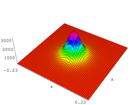
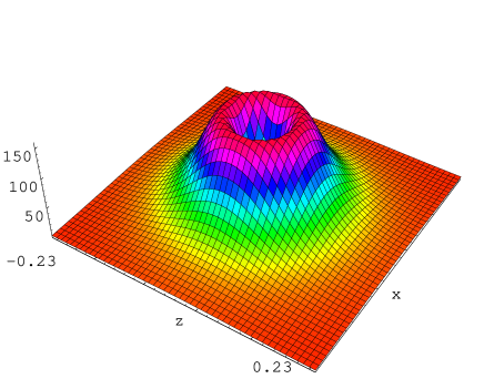
Figure 1: Supersymmetric (left) and non-supersymmetric (right) zero-mode densities for $\delta_{1}=0.2$ and $\rho=0.1$. Monopoles are localised on the z axis at $x=y=t=0$. Densities are plotted in the $x-z$ plane keeping $t=0$ and $y=0$. The lengths of the $x$ and $z$ axes are scaled by $4.6\rho$.

As illustration of the properties of the zero modes we show in Figs. (1)-(3) the densities of both supersymmetric and non supersymmetric zero modes for $\delta_{1}=0.2$ and several values of the scale parameter $\rho$. Densities are plotted in the $x-z$ plane keeping $t=0$ and $y=0$. For small $\rho$ the supersymmetric zero-mode reproduces the characteristic single-instanton shape. As $\rho$ increases the caloron dissociates into two constituent monopoles which tend, at large $\rho$, to two BPS monopoles. The non-supersymmetric mode has, at small $\rho$, a symmetric ring structure also characteristic of a normal instanton, going through zero at the center of mass of the caloron. The ring gets distorted as $\rho$ increases and dissociates for even larger $\rho$ into the two constituent BPS monopoles. This behaviour matches the one obtained analytically in the $\rho\rightarrow 0$ and $\rho\rightarrow\infty$ limits, which are described in the next section.

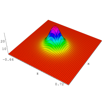
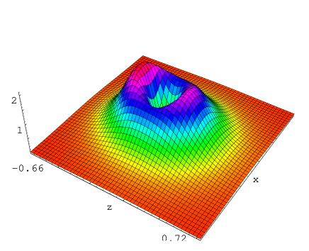
Figure 2: The same as in Fig. 1 but for $\rho=0.3$.

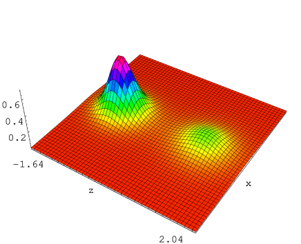
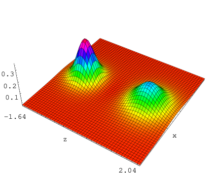
Figure 3: The same as in Fig. 1 but for $\rho=0.8$.

3 Properties of the solutions

In this section, we will clarify the spatial structure of the modes by studying their behaviour in certain limits. Since calorons interpolate between monopoles, instantons and HS calorons as one moves along the moduli space, a similar phenomenon is expected for the corresponding gluino zero-modes.

3.1 $\rho\longrightarrow\infty$ limit

There are several length scales involved in this problem ($m_{a}^{-1}$, the time period and the distance among constituents $\pi\rho^{2}$), so it is important to clarify precisely in what regime we are thinking of. We will consider the simplest situation in which $\pi\rho^{2}$ is much larger than all other length scales in the problem. In addition, we will focus on the behaviour close to one of the monopoles $r_{1}<<\pi\rho^{2}$. Then, for the other monopole one has $r_{2}\approx\pi\rho^{2}$.

All our expressions are built in terms of $V$ and $U_{a}$ (see Eqs. 59 and 60 in the appendix), so we will first analyse the behaviour of these quantities as a function of $\rho$. The quantity $U_{2}$ behaves for large distances as $r_{2}/2\pi\longrightarrow\rho^{2}/2$. Thus, $V$ becomes order $\rho^{-2}$. In order to compute the leading behaviour of F in this limit one has to keep the first correction as well. This is obtained by expanding

$$r_{2}=||\vec{r}_{1}-\pi\rho^{2}\vec{k}||=\pi\rho^{2}-(x_{3}-X^{1}_{3})+\ldots$$ (26)

In this way we arrive at

$$V=\frac{1}{\rho^{2}}(1-\frac{1}{\rho^{2}}(U_{1}-\frac{(x_{3}-X^{1}_{3})}{2\pi}))$$ (27)

and from here we see that $F$ is order $\rho^{2}$. From these results we conclude that $W$ (Eq. 58) is order $\rho^{-1}$, and $\hat{\partial}W$ of order $\rho^{-3}$ while the derivatives of $U_{a}$ are order 1. Then it is easy to see that, of the different terms contributing to the zero-modes, only the term proportional to the $a=1$ BPS monopole field is leading order. The latter is easily computable by realizing that the quantity inside parenthesis in Eq. 68 now becomes precisely $2/(F\rho^{2})$. This leads to $\lambda_{1}=1$ and $\lambda_{2}=0$. The conclusion is that for large separations and close to the center of the $a$th constituent monopole, the quantity $E_{i}^{a}$ is, after a performing a gauge rotation, simply given by the electric field of a single BPS monopole:

$$E^{\rm BPS}(\vec{x}-\vec{X}^{a};m_{a})$$ (28)

Now we recall that the integral of the BPS monopole electric field square over space equals $4\pi m$. We reproduce, in this limit, the well-known fact that the contribution of each constituent monopole to the energy will then become, at sufficiently large separation, proportional to $m_{1}$ and $m_{2}$ respectively. Adding the two contributions to get the supersymmetric mode gives a total integral of $8\pi^{2}$ as expected for the caloron.

Considering now the non-supersymmetric mode and taking into account that in Eq. 22 the first term is subleading in this limit, we conclude that the contribution of the $a$th constituent monopole to the total energy is given by $4\pi\rho^{4}m_{1}^{2}m_{2}^{2}/m_{a}$. This is consistent with the known result [1] about the integrated densities which appear when computing the metric of the caloron moduli space.

3.2 $\rho\longrightarrow 0$ limit

To be precise the limit is defined by the requirement that $m_{a}r_{a}<<1$ and the distances $r_{i}$ are of order $\rho$. This implies that in the first approximation one can neglect the separation between the constituent monopoles ($\pi\rho^{2}<<r_{i}$). As usual we will start by computing $U_{a}$ in this limit:

$$U_{a}=\pmatrix{\frac{m_{a}x^{2}}{4\pi}&\epsilon_{a}x_{0}\cr\epsilon_{a}x_{0}&\frac{1}{\pi m_{a}}}$$ (29)

where $x^{2}=x_{0}^{2}+r^{2}$ is the square of the 4d euclidean distance to the origin. Notice that the 11 element of this matrix is negligible with respect to the 22 element, but has to be kept to be able to compute the inverse matrix. From here we conclude that to leading order $V=2P_{11}/(x^{2}+\rho^{2})$, where $P_{11}$ is the matrix (projector) whose only non-vanishing component is 11, equal to 1. This projector appears in all our formulas and simplifies all vectors and matrices into single component. Using this it is easy to estimate the contribution of both terms in the expression for $E_{\mu}^{a}$, Eq. 70. The second term turns out to be subleading with respect to the first one. Using $\hat{\partial}(U_{1}+U_{2})=\hat{x}$ the second term in this equation gives:

$$\frac{im_{a}}{2\pi}\frac{\rho^{2}}{(x^{2}+\rho^{2})^{2}}\frac{\hat{x}\bar{\sigma}_{\mu}\hat{x}}{x^{2}}+h.c.$$ (30)

which is proportional ($m_{a}/(2\pi)$) to the gauge field of an instanton in a certain gauge. Hence, adding the $a=1$ and $a=2$ contributions, we conclude that the supersymmetric zero mode reduces in this limit to the one of an BRST instanton. Notice however that the combination of Eq. 30 entering in the non-supersymmetric zero mode vanishes.

For the case of the non-supersymmetric zero mode the leading term turns out to be the one proportional to the vector potential. For it we obtain

$$\frac{A_{\mu}}{F}\longrightarrow-i\frac{\rho^{2}}{2(x^{2}+\rho^{2})^{2}}\bar{\sigma}_{\mu}\hat{x}+\mbox{\rm h.c.}$$ (31)

Notice that this is precisely proportional to the well-known non-supersymmetric adjoint mode for the BRST instanton.

In summary, in this limit both adjoint modes tend to the corresponding ones for a BRST instanton.

4 Conclusions

In this paper we have derived, following the ADHM formalism, the analytic expressions for the gluino zero-modes of the Dirac operator in the background of topological charge 1 calorons with non-trivial holonomy. These gluino zero-modes are relevant for semiclassical studies of 4D Super-symmetric Yang-Mills theories. They can also turn out to be useful for analysing the structure and topological content of the QCD vacuum. In particular they can give a handle in the identification of constituent monopoles inside instantons, a subject that has recently received much attention [13]-[20].

For $Q=1$ there are four linearly independent zero modes which come in pairs related by Euclidean CP transformations. Two of them correspond to the super-symmetric zero modes and share the property that their density exactly reproduces the action density of the caloron. The other two modes show a quite distinct behaviour. For small scale parameter $\rho$ they have the same ring structure as for trivial calorons or instantons as exhibited in Fig. 1. As we increase $\rho$ the non-supersymmetric zero-mode rings get distorted (Fig. 2). For much larger $\rho$ both zero mode densities dissociate into two structures having the density profiles of BPS monopoles of masses $M_{1}$ and $M_{2}$ (Fig. 3). For the supersymmetric case the integrated contribution of each monopole to the energy is proportional to its mass. However, for the non supersymmetric modes these contributions are inversely proportional to their masses. By taking appropriate linear combinations it is possible to construct zero modes which, for intermediate to large scale parameters, single out only one of the two constituent monopoles.

All these features can certainly help in the identification of constituent monopoles in lattice generated ensembles. This identification has been up to now performed solely on the basis of the action density and the properties of fundamental zero-modes [13, 18], [19], becoming particularly complicated for low temperatures [20]. Adjoint zero modes provide an additional tool for this analysis. The supersymmetric zero mode density gives an estimate of the action density of the gauge field itself which is less sensitive to ultraviolet divergences.

Our present results can be extended to the case of SU(N) Q=1 calorons and to higher charge calorons. Furthermore, it is also possible to use our techniques to construct gluino zero-modes which are anti-periodic in time, directly relevant for finite temperature ${\cal N}=1$ supersymmetry [32].

5 Appendix

In this appendix we will present the derivation the analytic formulas of the zero modes given in the text. All interesting quantities are expressed in terms of the functions $u$ and $\omega$ (see Eqs. 11-10), and their integrals over z. These functions belong to a 4 dimensional vector space over the field of quaternions. The space is the direct sum of the spaces of functions annihilated (up to delta functions) by the operator $\widetilde{M}\equiv\widetilde{A}-\hat{x}$ and its adjoint. To obtain a basis of this space one must consider the functions

$$\Psi^{(+)}(z,x,\delta)=\chi(-\delta,\delta)\,e^{i2\pi\bar{x}z}$$ (32)

$$\Psi^{(-)}(z,x,\delta)=\chi(-\delta,\delta)\,e^{i2\pi\hat{x}z}$$ (33)

They are to be taken as periodic over $z$ ( and $x_{0}$) with unit period. The function $\chi(-\delta,\delta)$ is the characteristic function over the interval. In terms of these functions we can compute the 4 elements of the basis of the space:

$$\Psi^{\pm}_{a}\equiv\Psi^{(\pm)}(z-Z^{a},x-X^{a},\frac{m_{a}}{4\pi})$$ (34)

The index $a$ takes two values (1 and 2), which can be thought as labelling the two constituent monopoles. Indeed, $X^{a}$ stands for the location and $m_{a}=4\pi\delta_{a}$ for the mass (for $g^{2}=4\pi$) of each of the monopoles. The remaining coefficients are $Z^{1}=0$ and $Z^{2}=\frac{1}{2}$.

To derive the formulas one needs to know how the operators $\widetilde{M}$ and $\widetilde{M}^{\dagger}$ act on them. These are given by

$$\widetilde{M}^{\dagger}\Psi_{a}^{+} = \frac{-1}{2\pi}\left((e^{a}_{1}+ie^{a}_{2})\delta(z-\delta_{1})+(e^{a}_{1}-ie^{a}_{2})\delta(z+\delta_{1})\right)$$ (35)

$$\widetilde{M}\Psi_{a}^{-} = \frac{-1}{2\pi}\left((\bar{e}^{a}_{1}+i\bar{e}^{a}_{2})\delta(z-\delta_{1})+(\bar{e}^{a}_{1}-i\bar{e}^{a}_{2})\delta(z+\delta_{1})\right)$$ (36)

$$(\widetilde{M}-\widetilde{M}^{\dagger})\Psi_{a}^{\pm} = 2i(\vec{x}-\vec{X}^{a})\vec{\tau}\,\Psi_{a}^{\pm}$$ (37)

The quantities $e^{a}_{1}$ and $e^{a}_{2}$ are simple quaternionic functions of $x$ defined by the value of the basis functions at the extreme of the interval:

$$\lim_{z\rightarrow\delta_{1}^{-}}\Psi_{a}^{+}(z)=i\epsilon_{a}(e^{a}_{1}+ie^{a}_{2})\equiv(\bar{e}^{\prime a}_{1}+i\bar{e}^{\prime a}_{2})$$ (38)

where $\epsilon_{1}=-1$ and $\epsilon_{2}=1$, and we have introduced new quaternionic quantities $e^{\prime a}_{1}$, $e^{\prime a}_{2}$. In all expressions a bar over a quaternion denotes its adjoint.

All of the necessary functions of $z$ entering the caloron formulas can be expressed in terms of these functions. From the equations that they satisfy (Eq. 11, 10) we can easily deduce the general structure

$$u = \sum_{a}u_{a}=\sum_{a}(\Psi_{a}^{+}A_{a})$$ (39)

$$\omega = \sum_{a}(\Psi_{a}^{+}D_{a}^{(+)}+\Psi_{a}^{-}D_{a}^{(-)})$$ (40)

where the coefficients ($A_{a}$, $D_{a}^{\pm)}$, etc) are quaternionic functions of space-time.

For all the necessary calculations of adjoint modes one also needs the general form of $\hat{\partial}\omega$:

$$\hat{\partial}\omega=\sum_{a}(4\pi i(z-Z^{a})\Psi_{a}^{+}D_{a}^{(+)}+\Psi_{a}^{+}S_{a}^{(+)}+\Psi_{a}^{-}S_{a}^{(-)})$$ (41)

Finally, we need to know the integrals of the basis functions over $z$. We will need:

$$I^{\pm}_{\alpha}=\int dz\Psi_{b}^{+\dagger}\bar{\sigma}_{\alpha}\Psi_{a}^{\pm}=\delta_{ab}\frac{m_{a}}{2\pi}({\cal P}^{a\,\alpha}_{\pm}\frac{1}{g(m_{a}r_{a})}+{\cal P}^{a\,\alpha}_{\mp})$$ (42)

and

$$\widetilde{I}_{\alpha}=4\pi i\int dzz\Psi_{b}^{+\dagger}\bar{\sigma}_{\alpha}\Psi_{a}^{+}=-\frac{m_{a}^{2}}{2\pi}\left(\frac{g^{\prime}(m_{a}r_{a})}{g^{2}(m_{a}r_{a})}\right){\cal P}^{a\,\alpha}_{+}(i\hat{n}_{a})$$ (43)

where we have introduced the quaternions

$${\cal P}^{a\,\alpha}_{\pm}=\frac{1}{2}(\bar{\sigma}^{\alpha}\pm\hat{n}_{a}\bar{\sigma}^{\alpha}\hat{n}_{a})$$ (44)

The symbol $\hat{n}_{a}$ stands for a hermitian unitary traceless matrix defined through the decomposition

$$(\vec{x}-\vec{X}^{a})\vec{\tau}=r_{a}\hat{n}_{a}$$ (45)

where $r_{a}$ is the distance to the corresponding constituent monopole. The expressions also contain the function $g$:

$$g(u)=u/\sinh(u)$$ (46)

and its derivatives evaluated at the product of the mass and the distance.

With the previous expressions one can compute the caloron vector potential as well as the adjoint modes, once the coefficients $D^{(\pm)}_{a}$ and $S_{a}^{(\pm)}$ are known. These can be deduced from the equations that define $u$ and $\omega$ (Eqs. 11 and 10), but now the whole analytic structure reduces to a finite-dimensional linear problem in quaternions. Essentially, this follows from the matching at the edges of the intervals $z=\pm\delta_{1}$. For example, the absence of derivatives of delta functions in the equation for $\omega$, implies that this function must me continuous at $z=\pm\delta_{1}$. If we note $\omega(\delta_{1})=W_{1}+iW_{2}$, then we can compute the coefficients of $u$ and $\omega$ in terms of $W_{i}$ by the continuity equations:

$$W = \bar{e}^{\prime a}D_{a}^{(+)}+e^{\prime a}D_{a}^{(-)}$$ (47)

$$\hat{\partial}W = -4\pi\delta_{a}e^{a}D_{a}^{(+)}+\bar{e}^{\prime a}S_{a}^{(+)}+e^{\prime a}S_{a}^{(-)}$$ (48)

The equation has been rewritten as a vector equation in terms of two (quaternionic) component column vectors $W$, $e^{\prime a}$, $\ldots$ . Notice that each equation is valid for both values of $a$. With ordinary vector space techniques one can solve for the coefficients:

$$D_{a}^{(+)} = \frac{i\hat{n}_{a}g(m_{a}r_{a})}{m_{a}r_{a}}e^{a\dagger}W$$ (49)

$$D_{a}^{(-)} = \frac{-i\hat{n}_{a}g(m_{a}r_{a})}{m_{a}r_{a}}\bar{e}^{a\dagger}W$$ (50)

$$S_{a}^{(+)} = \frac{i\hat{n}_{a}g(m_{a}r_{a})}{m_{a}r_{a}}e^{a\dagger}\hat{\partial}W-\frac{m_{a}\cosh(m_{a}r_{a})}{\sinh^{2}(m_{a}r_{a})}e^{a\dagger}W$$ (51)

$$S_{a}^{(-)} = \frac{-i\hat{n}_{a}g(m_{a}r_{a})}{m_{a}r_{a}}\bar{e}^{a\dagger}\hat{\partial}W+\frac{m_{a}}{\sinh^{2}(m_{a}r_{a})}e^{a\dagger}W$$ (52)

The coefficient $A_{a}$ appearing in the expansion of $u$ can be related to $D_{a}^{(+)}$ by the equation $\widetilde{M}\omega=u/F$. Hence, we get

$$A_{a}=2ir_{a}F\hat{n}_{a}D_{a}^{(+)}$$ (53)

Combining all the previous formulas we arrive at

$$u_{a}^{\dagger}\bar{\sigma}_{\alpha}\hat{\partial}\omega_{a}=W^{\dagger}{\cal L}_{a\alpha}W+W^{\dagger}\widetilde{{\cal L}}_{a}\bar{\sigma}_{\alpha}\hat{\partial}W$$ (54)

where

$${\cal L}_{a\alpha}=\frac{2Fm_{a}g(m_{a}r_{a})}{\pi}e^{a}\left(-i\frac{g^{2}(m_{a}r_{a})-1}{2m_{a}^{2}r_{a}^{2}}{\cal P}^{a\,\alpha}_{+}-i\frac{g^{\prime}(m_{a}r_{a})}{2m_{a}r_{a}}{\cal P}^{a\,\alpha}_{-}\right)e_{a}^{\dagger}$$ (55)

and

$$\widetilde{{\cal L}}_{a}=\frac{-iFg(m_{a}r_{a})}{\pi m_{a}r_{a}}e_{a}\hat{n}_{a}\left(-g(m_{a}r_{a})\bar{e}_{a}^{\dagger}+e_{a}^{\dagger}\right)$$ (56)

Up to this point all expressions seem to depend only on a single distance $r_{a}$. The mixing among the two coordinates and the relation between the constituent monopoles is hidden in the expression of $W$. The main equation satisfied by $W$ is

$$\frac{F}{\pi}\sum_{a}\frac{g(m_{a}r_{a})}{m_{a}}e_{a}e_{a}^{\dagger}W=\frac{\rho}{2}\pmatrix{1\cr-i\tau_{3}}$$ (57)

From here one can solve for $W$. It is very easy to realise that $W$ must be a linear combination of the quaternion $i\tau_{3}$ and unity. This follows from the equation $\omega=R^{-1}q$. Since $q$ is a combination of these two quaternions and $R$ commutes with quaternions (and is therefore real), this property extends to $W$. In summary, we have

$$W=\frac{\rho}{2}V\pmatrix{1\cr-i\tau_{3}}$$ (58)

where V is a real $2\times 2$ matrix, whose inverse is sum of contributions from the two constituent monopoles

$$V^{-1}=\frac{\rho^{2}}{2}+\sum_{a}U_{a}$$ (59)

with

$$U_{a}=\frac{g(m_{a}r_{a})}{2\pi m_{a}}\pmatrix{\cosh(m_{a}r_{a})-\cos(m_{a}x_{0})&\epsilon_{a}\sin(m_{a}x_{0})\cr\epsilon_{a}\sin(m_{a}x_{0})&\cosh(m_{a}r_{a})+\cos(m_{a}x_{0})}$$ (60)

An interesting relation between $U$ and the vectors $e^{a}$ is given by

$$U_{a}=\frac{1}{\pi}\frac{g(m_{a}r_{a})}{m_{a}}e_{a}e_{a}^{\dagger}-\frac{\epsilon_{a}r_{a}}{2\pi}\pmatrix{0&i\hat{n}_{a}\cr-i\hat{n}_{a}&0}$$ (61)

Now we have all the ingredients to calculate all the relevant quantities concerning calorons, including the adjoint zero-modes. For example, we can obtain the scalar function $F$

$$F=\frac{1}{1-\rho^{2}\mbox{ \rm Tr}(V)/2}$$ (62)

For the vector potential, we can write the following expression:

$$A_{\mu}=\frac{-iF}{2}W^{\dagger}\bar{\sigma}_{\mu}\hat{\partial}(U_{1}+U_{2})\,W+\mbox{ \rm h. c. }$$ (63)

Finally, we proceed to the computation of the basic quantity which enters into the expression of the zero modes $E^{a}_{\alpha}(x)$. This is obtained from Eq. 54 after multiplying by $i$ and taking the hermitian part. The result is the sum of two terms. The first one has a very transparent interpretation. To show this, one must first realize that the traceless part (or hermitian part) of the quantity inside parenthesis in Eq. 55 is precisely $E^{\rm BPS}_{\alpha}(x-X^{a};m_{a})/m_{a}^{2}$, where $E^{\rm BPS}_{\alpha}(x-X^{a};m_{a})$ is the gauge field of a BPS monopole of mass $M_{a}$ centered at one of the constituent monopoles. This is sandwiched between the quaternion $Q_{a}\equiv e^{a\dagger}W$ and its adjoint. If we write

$$Q_{a}\equiv e^{a\dagger}W=|Q_{a}|\Omega^{\dagger}_{a}$$ (64)

where $\Omega_{a}$ is a unitary matrix and we define

$$\lambda_{a}=|Q_{a}|^{2}\frac{2Fg_{a}}{\pi m_{a}}$$ (65)

then we conclude that the first term in $E^{a}_{\alpha}(x)$ is given by

$$\lambda_{a}\Omega_{a}E^{\rm BPS}_{\alpha}(x-X^{a};m_{a})\Omega_{a}^{\dagger}$$ (66)

which is just the field of a BPS monopole, gauge rotated and weighted by $\lambda_{a}$. The weight factors are positive and satisfy:

$$\sum_{a}\lambda_{a}=(1-\frac{1}{F})$$ (67)

An explicit formula to compute them in terms of the matrix $V$ is

$$\lambda_{a}=\frac{F\rho^{2}}{2}\left(\mbox{\rm Tr}(VU_{a}V)+\frac{\epsilon_{a}}{2\pi}(x_{3}-X_{3}^{a})(\mbox{\rm Tr}^{2}(V)-\mbox{\rm Tr}(V^{2}))\right)$$ (68)

The second piece contributing to Eq. 54 is also simplified if one realizes that

$$\widetilde{{\cal L}}_{a}=-F\bar{\partial}U_{a}$$ (69)

Hence, one reaches to the following simple formula for the quantity $E^{a}_{\mu}$, representing the contribution of constituent monopole $a$ to the field strength

$$E^{a}_{\mu}=\frac{Fg(m_{a}r_{a})}{\pi m_{a}}W^{\dagger}e^{a}E^{\rm BPS}_{\mu}(x-X^{a};m_{a})\,e^{a\dagger}W-\frac{iF}{2}W^{\dagger}\bar{\partial}U_{a}\bar{\sigma_{\mu}}\hat{\partial}W+\mbox{\rm h.c.}$$ (70)

The time-like component ($\mu=0$) of the first term vanishes. For the second term we have $E^{1}_{0}=-E^{2}_{0}$. This is easily concluded by realizing that

$$\hat{\partial}W=-V\hat{\partial}(U_{1}+U_{2})W$$ (71)

References

- [1] T. C. Kraan and P. van Baal, Phys. Lett. B 428 (1998) 268 [arXiv:hep-th/9802049]. Nucl. Phys. B 533 (1998) 627 [arXiv:hep-th/9805168].
- [2] T. C. Kraan and P. van Baal, Phys. Lett. B 435 (1998) 389 [arXiv:hep-th/9806034].
- [3] K. M. Lee, Phys. Lett. B 426 (1998) 323 [arXiv:hep-th/9802012].
- [4] K. M. Lee and C. h. Lu, Phys. Rev. D 58, 025011 (1998) [arXiv:hep-th/9802108].
- [5] F. Bruckmann and P. van Baal, Nucl. Phys. B 645, 105 (2002) [arXiv:hep-th/0209010]. F. Bruckmann, D. Nogradi and P. van Baal, Nucl. Phys. B 698 (2004) 233 [arXiv:hep-th/0404210].
- [6] B. J. Harrington and H. K. Shepard, Phys. Rev. D 17, 2122 (1978). Phys. Rev. D 18 (1978) 2990.
- [7] P. Rossi, Phys. Rept. 86 (1982) 317.
- [8] A. A. Belavin, V. A. Fateev, A. S. Schwarz and Y. S. Tyupkin, Phys. Lett. B 83 (1979) 317.
- [9] C. G. . Callan, R. F. Dashen and D. J. Gross, Phys. Rev. D 17 (1978) 2717.
- [10] M. Garcia Perez, A. Gonzalez-Arroyo and B. Soderberg, Phys. Lett. B 235 (1990) 117. M. Garcia Perez and A. Gonzalez-Arroyo, J. Phys. A 26 (1993) 2667 [arXiv:hep-lat/9206016].
- [11] G. ’t Hooft, Nucl. Phys. B 153 (1979) 141.
- [12] M. Garcia Perez, A. Gonzalez-Arroyo and P. Martinez, Nucl. Phys. Proc. Suppl. 34 (1994) 228 [arXiv:hep-lat/9312066]. A. Gonzalez-Arroyo and P. Martinez, Nucl. Phys. B 459 (1996) 337 [arXiv:hep-lat/9507001]. A. Gonzalez-Arroyo, P. Martinez and A. Montero, Phys. Lett. B 359 (1995) 159 [arXiv:hep-lat/9507006]. A. Gonzalez-Arroyo and A. Montero, Phys. Lett. B 387 (1996) 823 [arXiv:hep-th/9604017].
- [13] C. Gattringer, Phys. Rev. D 67 (2003) 034507 [arXiv:hep-lat/0210001]. C. Gattringer and S. Schaefer, Nucl. Phys. B 654 (2003) 30 [arXiv:hep-lat/0212029].
- [14] E. M. Ilgenfritz, B. V. Martemyanov, M. Muller-Preussker, S. Shcheredin and A. I. Veselov, Phys. Rev. D 66 (2002) 074503 [arXiv:hep-lat/0206004]. E. M. Ilgenfritz, M. Muller-Preussker and D. Peschka, Phys. Rev. D 71 (2005) 116003 [arXiv:hep-lat/0503020]. E. M. Ilgenfritz, B. V. Martemyanov, M. Muller-Preussker and A. I. Veselov, Phys. Rev. D 71 (2005) 034505 [arXiv:hep-lat/0412028]. E. M. Ilgenfritz, B. V. Martemyanov, M. Muller-Preussker and A. I. Veselov, arXiv:hep-lat/0602002.
- [15] N. M. Davies, T. J. Hollowood, V. V. Khoze and M. P. Mattis, Nucl. Phys. B 559 (1999) 123 [arXiv:hep-th/9905015].
- [16] M. Garcia Perez, A. Gonzalez-Arroyo, C. Pena and P. van Baal, Phys. Rev. D 60 (1999) 031901 [arXiv:hep-th/9905016]. M. Garcia Perez, A. Gonzalez-Arroyo, A. Montero and P. van Baal, JHEP 9906 (1999) 001 [arXiv:hep-lat/9903022].
- [17] M. N. Chernodub, T. C. Kraan and P. van Baal, Nucl. Phys. Proc. Suppl. 83 (2000) 556 [arXiv:hep-lat/9907001]. F. Bruckmann, D. Nogradi and P. van Baal, Nucl. Phys. B 666 (2003) 197 [arXiv:hep-th/0305063].
- [18] C. Gattringer and R. Pullirsch, Phys. Rev. D 69 (2004) 094510 [arXiv:hep-lat/0402008]. C. Gattringer and S. Solbrig, Nucl. Phys. Proc. Suppl. 152 (2006) 284 [arXiv:hep-lat/0410040].
- [19] E. M. Ilgenfritz, B. V. Martemyanov, M. Muller-Preussker and A. I. Veselov, Phys. Rev. D 69 (2004) 114505 [arXiv:hep-lat/0402010].
- [20] F. Bruckmann, E. M. Ilgenfritz, B. V. Martemyanov and P. van Baal, Phys. Rev. D 70 (2004) 105013 [arXiv:hep-lat/0408004].
- [21] E. Cohen and C. Gomez, Phys. Rev. Lett. 52 (1984) 237.
- [22] S. J. Hands and M. Teper, Nucl. Phys. B 347 (1990) 819.
- [23] I. Horvath et al., Phys. Rev. D 66 (2002) 034501 [arXiv:hep-lat/0201008].
- [24] C. Gattringer, M. Gockeler, C. B. Lang, P. E. L. Rakow and A. Schafer, Phys. Lett. B 522 (2001) 194 [arXiv:hep-lat/0108001].
- [25] T. A. DeGrand and A. Hasenfratz, Phys. Rev. D 65 (2002) 014503 [arXiv:hep-lat/0103002].
- [26] H. Neuberger, Phys. Rev. Lett. 81 (1998) 4060 [arXiv:hep-lat/9806025]; Phys. Lett. B 427 (1998) 353 [arXiv:hep-lat/9801031]; Phys. Lett. B 417 (1998) 141 [arXiv:hep-lat/9707022].
- [27] A. Gonzalez-Arroyo and R. Kirchner, JHEP 0601 (2006) 029 [arXiv:hep-lat/0507036].
- [28] M. F. Atiyah, N. J. Hitchin, V. G. Drinfeld and Y. I. Manin, Phys. Lett. A 65 (1978) 185.
- [29] H. Osborn, Nucl. Phys. B 159 (1979) 497; Annals Phys. 135 (1981) 373.
- [30] W. Nahm, Phys. Lett. B 90 (1980) 413; “All Selfdual Multi - Monopoles For Arbitrary Gauge Groups,” CERN-TH-3172 Presented at Int. Summer Inst. on Theoretical Physics, Freiburg, West Germany, Aug 31 - Sep 11, 1981
- [31] T. C. Kraan, Commun. Math. Phys. 212 (2000) 503 [arXiv:hep-th/9811179].
- [32] F. Bruckmann, M. García Pérez and A. González-Arroyo, in preparation.