CU-TP-1155

KIAS-P06041

hep-th/0609055

Magnetic Monopole Dynamics, Supersymmetry, and Duality

Erick J. Weinberg^a,b and Piljin Yi^b

^aPhysics Department, Columbia University, New York, N.Y. 10027, U.S.A.

^bSchool of Physics, Korea Institute for Advanced Study,

207-43, Cheongnyangni-2dong, Dongdaemun-gu, Seoul 130-722, Korea

We review the properties of BPS, or supersymmetric, magnetic monopoles, with an emphasis on their low-energy dynamics and their classical and quantum bound states.

After an overview of magnetic monopoles, we discuss the BPS limit and its relation to supersymmetry. We then discuss the properties and construction of multimonopole solutions with a single nontrivial Higgs field. The low-energy dynamics of these monopoles is most easily understood in terms of the moduli space and its metric. We describe in detail several known examples of these. This is then extended to cases where the unbroken gauge symmetry include a non-Abelian factor.

We next turn to the generic supersymmetric Yang-Mills (SYM) case, in which several adjoint Higgs fields are present. Working first at the classical level, we describe the effects of these additional scalar fields on the monopole dynamics, and then include the contribution of the fermionic zero modes to the low-energy dynamics. The resulting low-energy effective theory is itself supersymmetric. We discuss the quantization of this theory and its quantum BPS states, which are typically composed of several loosely bound compact dyonic cores.

We close with a discussion of the D-brane realization of ${\cal N}=4$ SYM monopoles and dyons and explain the ADHMN construction of monopoles from the D-brane point of view.

Chapter 1 Introduction

The magnetic monopole may be the most interesting, and perhaps the most important, particle to be never found.

Once the unity of electricity and magnetism was understood, it was quite natural to conjecture the existence of isolated magnetic poles that would be the counterparts of electric charges and that would complete the electric-magnetic duality of Maxwell’s equation. Interest in the possibility of such objects was increased by Dirac’s observation in 1931 [1] that the existence of even a single magnetic monopole would provide an explanation for the observed quantization of electric charge.

A new chapter opened in 1974, when ’t Hooft [2] and Polyakov [3] showed that in certain spontaneously broken gauge theories — a class that includes all grand unified theories — magnetic monopoles are not just a possibility, but a prediction. These objects are associated with solutions of the corresponding classical field equations and, in the weak coupling regime, their mass and other properties are calculable.

These theoretical developments were accompanied by experimental searches for monopoles in bulk matter (including rocks from the Moon) and cosmic rays as well as by attempts to produce them in particle accelerators. To date all of these have been negative, and theoretical arguments now suggest, at least for GUT monopoles, that their abundance in the universe is so low as to make the detection of even one to be extraordinarily unlikely. Already in 1981, Dirac wrote [4], in response to an invitation to a conference on the fiftieth anniversary of his paper,

“I am inclined now to believe that monopoles do not exist. So many years have gone by without any encouragement from the experimental side.”

Yet, in the half-decade preceeding Dirac’s statement magnetic monopoles had inspired two important lines of theoretical inquiry. First, the attempt to understand why there is not an overabundance of monopoles surviving from the early universe [5] led Guth to the inflationary universe scenario [6], which has revolutionized our understanding of cosmology. The second direction, initiated by the approximation introduced by Prasad and Sommerfield [7] and by Bogomolny [8], has led to considerable insights into the properties of supersymmetric field theories and string theory. It is this latter line of research that is the subject of this review.

The Bogomolny-Prasad-Sommerfield (BPS) limit of vanishing scalar potential was first proposed simply as a means of obtaining an analytic expression for the classical monopole solution. However, over the next few years several remarkable properties of the theory in this limit emerged. First, it was shown that solutions of the full second-order field equations could be obtained by solving the Bogomolny equation, a kind of self-duality equation that is first order in the fields. Solutions of this equation are guaranteed to have an energy that is exactly proportional to the magnetic charge. This suggests that there might be static solutions composed of two or more separated monopoles, with their mutual magnetic repulsion exactly cancelled by the attractive force mediated by the Higgs field, which becomes massless in the BPS limit. This possibility is actually realized, with there being continuous families of multimonopole solutions.

In the context of the classical SU(2) theory, the BPS limit seems to be rather ad hoc, and the properties that follow from it appear to be curiosities with no deep meaning. Their relevance for the quantum theory seems uncertain. Indeed, it is not even clear that the BPS limit can be maintained when quantum corrections are included. However, matters are clarified by the realization that this theory can be naturally expanded in a way that makes it supersymmetric. The resulting supersymmetric Yang-Mills (SYM) theory has a nonvanishing scalar field potential — whose form is preserved by quantum corrections — but yet yields the same classical field equations. The classical energy-charge relation is seen to correspond to an operator relation between the Hamiltonian and the central charges, with states obeying this relation lying in a special class of supermultiplets and leaving unbroken some of the generators of the supersymmetry. This relation implies the Bogomolny equation in the weak coupling limit, but is still meaningful when the coupling is so large that the semiclassical approximation can no longer be trusted.

There is another motivation for making the theory supersymmetric. Montonen and Olive [9] had noted that the classical mass spectrum was invariant under an electric-magnetic duality symmetry, and suggested that this might be a symmetry of the full theory. However, when particle spins are taken into account, the spectrum is seen to only be fully invariant if the theory is maximally expanded, to ${\cal N}=4$ SYM. If the field theory is viewed as a low-energy approximation to string theory, this duality symmetry is a reflection of the S-duality of the string theory.

The supersymmetry brings in other new features. If the gauge group is larger than SU(2), the additional scalar fields of the SYM theory give rise to new classical solutions that can be viewed as loosely bound collections of two or more dyonic cores. These can be studied within the quantum theory with the aid of a low-energy effective theory. This is a truncation of the full quantum field theory that retains only the bosonic collective coordinates of the individual monopoles and their fermionic counterparts associated with fermion zero modes. The correspondence between the classical and quantum theories turns out to be rather subtle, revealing some unexpected aspects of the spectra of supersymmetric, or BPS, states in SYM theories.

The spectrum of BPS states becomes of particular importance in the context of duality, both in field theory and in string theory. In the 1990’s, as the notion of duality took on a more definite formulation, the study of the BPS spectra became a primary tool for checking whether a duality existed between a pair of theories. This was true not only for the self-duality of ${\cal N}=4$ SYM field theory, but for the various dualities between the five string theories in ten dimensions and M theory in eleven dimensions, where supersymmetric states involving D-branes are often counted and matched with their dual BPS states.

Although the initial investigations in this direction were fairly successful, the counting of more general BPS states turned out to be anything but straightforward. This was particularly true for those BPS states that preserve four or fewer supercharges. The existence of such states is often sensitive to the choice of vacuum and to the choice of coupling constants, which are then interwoven with the duality in a subtle manner. So far, no general theory of BPS spectra is known, although much effort has been devoted to attacking this problem in the many guises in which it presents itself, including D-branes wrapping cycles in Calabi-Yau manifolds, boundary states in conformal field theories, open membranes ending on appropriately curved M5 branes, and BPS dyons in the Seiberg-Witten description of ${\cal N}=2$ SYM.

We believe the material presented in this review will shed much light on this general unsolved problem. While the methodology used here is itself somewhat limited, in that it deals with weakly coupled SYM, some of the qualitative features should prove to be common to all these related problems. These include both the marginal stability domain wall and the large degeneracy, unrelated to any known symmetry, that is often found in BPS states with large charges.

We begin our review, in Chap. 2, with an overview of the SU(2) magnetic monopole solution of ’t Hooft and Polyakov. We describe how it arises as a topological soliton. We also discuss the zero modes about the solution, and explain how one of these, related to the unbroken global gauge symmetry, leads to the existence of dyonic solutions carrying both electric and magnetic charges. We introduce the moduli space of solutions and its metric; these concepts play an important role in our later discussions.

In Chap. 3, we specialize to the case of BPS solutions. We discuss in detail their relation to supersymmetry, and describe how magnetically charged states that preserve part of the supersymmetry can be obtained. The Montonen-Olive duality conjecture is also introduced here.

Chapter 4 is devoted to the discussion of classical multimonopole solutions. After developing the formalism for describing monopoles in theories with gauge groups larger than SU(2), we show how index theory methods can be used to determine the dimension of the space of solutions. We describe a powerful method, introduced by Nahm, for constructing multimonopole solutions and illustrate its use with several examples.

For a given magnetic charge, the multimonopole solutions obtained in Chap. 4 form a manifold, the moduli space, with the coordinates on this manifold naturally taken to be the collective coordinates of the component monopoles. In the low-energy limit, a good approximation to the full field theory dynamics is obtained by truncating to these collective coordinates, whose behavior is governed by a purely kinetic Lagrangian that is specified by a naturally defined metric on the moduli space. The classical motions of the monopoles correspond to geodesics on the moduli space. We discuss the moduli space and its metric in Chap. 5, and describe, with examples, some methods by which the metric can be determined.

Most of the discussion in this review assumes that the gauge group is maximally broken, to a product of U(1)’s. In Chap. 6 we discuss some of the consequences of the alternate possibility, where there is an unbroken non-Abelian subgroup. Among these are the presence of “massless monopoles” that are the dual counterparts of the massless gauge bosons and their superpartners. These massless monopoles cannot be realized as isolated classical solitons, but are instead found as clouds of non-Abelian field surrounding one or more massive monopoles.

Although SYM theories with extended supersymmetry contain either two (for ${\cal N}=2$) or six (for ${\cal N}=4$) Higgs fields, the discussion of classical solutions up to this point assumes that only one of these is nontrivial. For an SU(2) gauge theory this can always be arranged by a redefinition of fields. However, for larger gauge groups it need not be the case, a point that was fully appreciated only relatively recently. The generic solution then has two nontrivial Higgs fields, and is typically a dyonic bound state with components carrying both magnetic and electric charges. The BPS solutions preserve only one-fourth, rather than one-half, of the supersymmetry. The low-energy dynamics can still be described in terms of the collective coordinates and the moduli space that they span, but the moduli space Lagrangian now includes a potential energy term. In Chap. 7 we discuss the effects of these additional scalar fields, and show how to derive the potential energy that they generate.

Although we are considering supersymmetric theories, the effects of the fermions have been omitted so far. This is remedied in Chap. 8, where we introduce fermionic counterparts to the bosonic collective coordinates, and derive the effects of the fermion fields on the low-energy dynamics. The resulting moduli space Lagrangian possesses a supersymmetry that is inherited from that of the underlying field theory. The discussions thus far, although being set in the context of a quantum field theory, have been essentially classical. In this chapter we also show how to quantize this low-energy Lagrangian.

In Chap. 9, we discuss the quantum BPS dyons that arise as bound states of this Lagrangian. In a sense, this is the quantum counterpart of the classical discussion of Chap. 7. We present the exact wavefunctions for several states comprising only two dyonic cores. Although it appears to be much more difficult to obtain explicit wavefunctions for states with many cores, we show how index theorems can be used to count such states. An important point that emerges here is the striking difference between the spectra of the ${\cal N}=2$ and ${\cal N}=4$ SYM theories. In particular, only the latter includes certain zero-energy bound states that are required to satisfy the duality conjecture for larger gauge groups.

Although the monopoles that we discuss arise originally in the context of field theory, they find a very natural setting when the quantum field theory is viewed as the low-energy limit of string theory. In Chap. 10, we describe how the monopoles and dyons of ${\cal N}=4$ SYM can be realized, in a rather elegant fashion, in terms of D-branes. In particular, we describe how this picture provides a very natural motivation for the multimonopole construction of Nahm.

There are two appendices. Appendix A provides some background material on complex geometry and zero modes. Appendix B describes the extension of the discussions of Chap. 8 to ${\cal N}=2$ SYM theories containing matter hypermultiplets.

Chapter 2 The SU(2) magnetic monopole

The first example of a magnetic monopole solution was discovered by ’t Hooft [2] and Polyakov [3], working in the context of an SU(2) gauge theory. Although many examples with larger gauge groups have subsequently been found, the SU(2) solution remains the simplest, and is perhaps the best suited for introducing some concepts that will be important for our subsequent discussions. Furthermore, this solution will play an especially fundamental role for us, because in the Bogomolny-Prasad-Sommerfield (BPS) [7, 8] limit the monopole solutions for larger groups are all built up, in a sense that will later become clear, from components that are essentially SU(2) in nature.

We start our discussion in Sec. 2.1, where we describe how nonsingular magnetic monopoles can arise as topological solitons, and then focus on the ’t Hooft-Polyakov solution in Sec. 2.2. These static solutions actually belong to continuous families of solutions, all with the same energy. In the one-monopole case considered in this chapter, these solutions are specified by four parameters, all related to the symmetries of the theory; in later chapters we will explore the much richer multimonopole structure that arises in the BPS limit. As we explain in Sec. 2.3, infinitesimal variations of these parameters are associated with zero modes about a given solution. Excitation of these modes gives rise to time-dependent monopole solutions. Translational zero modes thus give rise in a straightforward manner to solutions with nonzero linear momentum. The case of global gauge modes, which lead to dyonic solutions with nonzero electric charge [10], is somewhat more subtle, as we describe in Sec. 2.4. In Sec. 2.5 we describe how a family of degenerate static solutions can be viewed as forming a manifold, known as the moduli space, with a naturally defined metric. Although this concept is relatively trivial for the one-monopole solutions considered in this chapter, it proves to be a powerful tool for understanding the multimonopole solutions we will study in later chapters. Finally, in Sec. 2.6, we discuss the relevance of these classical soliton solutions for the quantum theory.

Our main focus in this chapter is on providing the background for the discussion for monopoles in the BPS limit. Of necessity, there are many other aspects of magnetic monopoles that we must omit. For further discussion of these, we refer the reader to two classic reviews [11, 12].

2.1 Magnetic monopoles as topological solitons

We consider an SU(2) gauge theory whose symmetry is spontaneously broken to U(1) by a triplet Higgs field $\Phi$. With the generalization to other gauge groups in mind, we will usually write the fields as Hermitian matrices in the fundamental representation of the group. However, for this SU(2) example it will sometimes be more convenient to work in terms of component fields defined by

$$A_{\mu}={1\over 2}\tau^{a}A_{\mu}^{a}\,,\qquad\qquad\Phi={1\over 2}\tau^{a}\Phi^{a}\,.$$ (2.1.1)

Our conventions will be such that $\Phi^{a}\Phi^{a}=2{\rm Tr\,}\Phi^{2}\equiv|\Phi|^{2}$.

The Lagrangian is

$${\cal L}=-{1\over 2}{\rm Tr\,}F_{\mu\nu}F^{\mu\nu}+{\rm Tr\,}D_{\mu}\Phi D^{\mu}\Phi-V(\Phi)$$ (2.1.2)

where

$$V(\Phi)=-\mu^{2}{\rm Tr\,}\Phi^{2}+\lambda({\rm Tr\,}\Phi^{2})^{2}\,,$$ (2.1.3)

$$D_{\mu}\Phi=\partial_{\mu}\Phi+ie[A_{\mu},\Phi]\,,$$ (2.1.4)

and

$$F_{\mu\nu}=\partial_{\mu}A_{\nu}-\partial_{\nu}A_{\mu}+ie[A_{\mu},A_{\nu}]\,.$$ (2.1.5)

It is often convenient to separate the field strength into magnetic and electric parts

$$B_{i}={1\over 2}\epsilon_{ijk}F_{jk}$$ (2.1.6)

and

$$E_{i}=F_{0i}\,.$$ (2.1.7)

In order that there be a lower bound on the energy, $\lambda$ must be positive. If $\mu^{2}>0$, as we will assume, there is a degenerate family of asymmetric classical minima with

$$|\Phi|=v\equiv\sqrt{\mu^{2}\over\lambda}\,.$$ (2.1.8)

These preserve only a U(1) subgroup, which we will describe with the language of electromagnetism.

For definiteness, let us choose the vacuum solution

$$\Phi(x) = v{\tau^{3}\over 2}\equiv\Phi_{0}$$ (2.1.9)

$$A_{\mu}(x) = 0$$ (2.1.11)

so that the unbroken U(1) corresponds to the “$a=3$” direction of the SU(2). The physical fields may then be taken to be

$${\cal A}_{\mu} = A_{\mu}^{3}$$ (2.1.12)

$$W_{\mu} = {A_{\mu}^{1}+iA_{\mu}^{2}\over\sqrt{2}}$$ (2.1.14)

$$\varphi = \Phi^{3}\,.$$ (2.1.16)

The corresponding elementary quanta are a massless “photon”, a pair of vector mesons with mass $m_{W}=ev$ and electric charges $\pm e$, and an electrically neutral scalar boson with mass $m_{H}=\sqrt{2}\,\mu$.

This theory also has nontrivial classical solutions. The existence of these can be demonstrated without having to examine the field equations in detail. The key fact is that any static configuration that is a local minimum of the energy is necessarily a solution of the classical field equations. Our strategy will be to identify a special class of finite energy configurations and then show that the configuration of minimum energy among these cannot be the vacuum.

It is fairly clear that in a finite energy solution the fields must approach a vacuum solution as $r\rightarrow\infty$ in any fixed direction. However, this need not be the same vacuum solution in every direction. Thus, we could allow

$$\lim_{r\rightarrow\infty}\Phi(r,\theta,\phi)\equiv\Phi_{\infty}(\Omega)=U(\Omega)\Phi_{0}U^{-1}(\Omega)$$ (2.1.17)

to vary with direction, provided that it is accompanied by a suitable asymptotic gauge potential. (Note that the smoothness of $\Phi$ does not imply that $U$ must be smooth. In the cases of most interest to us, $U$ has a singularity.) The function $\Phi_{\infty}(\Omega)$ is a continuous mapping of the two-sphere at spatial infinity onto the space of Higgs fields obeying Eq. (2.1.8), which happens to also be a two-sphere. Such maps can be classified into topologically distinct classes corresponding to the elements of the homotopy group $\Pi_{2}(S^{2})$. Any two maps within the same class can be continuously deformed one into the other, while two maps in different classes cannot.

One can show that $\Pi_{2}(S^{2})=Z$, the additive group of the integers, so that configurations can be labelled by an integer winding number

$$n={1\over 8\pi}\epsilon_{ijk}\,\epsilon_{abc}\int d^{2}S_{i}\,\hat{\phi}^{a}\,\partial_{j}\hat{\phi}^{b}\,\partial_{k}\hat{\phi}^{c}$$ (2.1.18)

where $\hat{\phi}^{a}$ is the unit vector $\Phi^{a}/|\Phi|$ and the integration is taken over a sphere at spatial infinity. In fact, since the value of the integral is quantized, it must be invariant under smooth deformations of the surface of integration that do not cross any of the zeroes of $\Phi$, where $\hat{\phi}^{a}$ is undefined. It follows that any configuration with nonzero winding number must have at least $|n|$ zeroes of the Higgs field (precisely $n$ if one distinguishes between zeroes and “antizeroes” and counts the latter with a factor of $-1$).

The vacuum solution of Eq. (2.1.11) clearly has $n=0$ and falls within the trivial, identity, element of the homotopy group.

Now consider the set of field configurations such that the Higgs field at spatial infinity has unit winding number, $n=1$. Among these configurations, there must be one with minimum energy. This cannot be a vacuum solution (because it has a different winding number) and cannot be smoothly deformed into the vacuum (because winding number is quantized). Hence, this configuration must be a local minimum of the energy and thus a static classical solution.

Some of the asymptotic properties of this solution can be obtained from general arguments. In order that the energy be finite, the asymptotic Higgs field must be of the form

$$\Phi^{a}=v{\hat{\phi}}^{a}\,.$$ (2.1.19)

Further, the covariant derivative $D_{i}\Phi$ must fall faster than $r^{-3/2}$, which implies that

$$\partial_{i}{\hat{\phi}}^{a}-e\,\epsilon_{abc}\,A_{i}^{b}\,\hat{\phi}^{c}<O(r^{-3/2})\,.$$ (2.1.20)

This in turn requires that the gauge potential be of the form

$$A_{i}^{a}={1\over e}\epsilon_{abc}\,\hat{\phi}^{b}\,\partial_{i}\hat{\phi}^{c}+f_{i}({\bf r})\hat{\phi}^{a}+\cdots$$ (2.1.21)

where the ellipsis represents terms that fall faster than $r^{-3/2}$.

The corresponding magnetic field is

$$B_{i}^{d}={1\over 2}\epsilon_{ijk}\left[{1\over e}\epsilon_{abc}\,\hat{\phi}^{a}\,\partial_{j}\hat{\phi}^{b}\,\partial_{k}\hat{\phi}^{c}+(\partial_{j}f_{k}-\partial_{k}f_{j})\right]\hat{\phi}^{d}+\cdots\,.$$ (2.1.22)

Its leading terms are proportional to ${\hat{\phi}}^{a}$ and thus lie in the “electromagnetic” U(1) defined by the Higgs field. We define the magnetic charge by

$$Q_{M}=\int d^{2}S_{i}\,\hat{\phi}^{a}\,B_{i}^{a}\,.$$ (2.1.23)

When Eq. (2.1.22) is inserted into this expression, the first term gives a contribution proportional to the winding number (2.1.18), which we are assuming to be unity, while the contribution from the second term vanishes as a consequence of Gauss’s theorem; hence, the solution corresponds to a magnetic monopole with charge $4\pi/e$. More generally [15], a solution with Higgs field winding number $n$ has a magnetic charge

$$Q_{M}={4\pi n\over e}\,.$$ (2.1.24)

The classical energy of the solution, which gives the leading approximation to the monopole mass, is

$$E=\int d^{3}x\left[{\rm Tr\,}E_{i}^{2}+{\rm Tr\,}(D_{0}\Phi)^{2}+{\rm Tr\,}B_{i}^{2}+{\rm Tr\,}(D_{i}\Phi)^{2}+V(\Phi)\right]\,.$$ (2.1.25)

For a static solution with no electric charge, one would expect the first two terms to vanish. The contribution of the remaining terms can be estimated by rewriting Eq. (2.1.25) in terms of the dimensionless quantities ${\bf s}=ev{\bf x}$, $\psi=\Phi/v$, and $a_{i}=A_{i}/v$. This isolates the dependence on $e$ and $v$, and shows that the mass must be of the form

$$M={4\pi v\over e}f(\lambda/e^{2})$$ (2.1.26)

where $f(\lambda/e^{2})$ is expected to be of order unity.

2.2 The ’t Hooft-Polyakov solution

In trying to proceed beyond this point, considerable simplification is achieved by restricting to the case of spherically symmetric solutions. In a gauge theory this means that the fields must be invariant under the combination of a naive rotation and a compensating gauge transformation, which may be position-dependent. With unit winding number, $n=1$, this position-dependence can be eliminated by adopting a special gauge choice that correlates the orientation of the Higgs field in internal space with the direction in physical space. In this “hedgehog” gauge, rotational invariance requires that the fields be invariant under combined rotation and global internal SU(2) transformation. This gives the ansatz

$$A_{i}^{a} = \epsilon_{iam}\hat{r}^{m}\left[1-u(r)\over er\right]$$ (2.2.1)

$$\Phi^{a} = \hat{r}^{a}h(r)$$ (2.2.2)

for the Higgs field and the spatial components of the gauge potential [2, 3]. It is easy to verify that for time-independent fields one can consistently set $A_{0}=0$ in the field equations, and we do so now.

The equations obeyed by $u$ and $h$ can be obtained either by substituting the ansatz (2.2.2) directly into the field equations, or by substituting it into the Lagrangian in Eq. (2.1.2) and then varying the resulting expression with respect to these coefficient functions. (The latter procedure is allowed because the ansatz is the most general one consistent with a symmetry of the Lagrangian.) Either way, one obtains

$$0 = h^{\prime\prime}+{2\over r}h^{\prime}-{2u^{2}h\over r^{2}}+\lambda(v^{2}-h^{2})h$$ (2.2.3)

$$0 = u^{\prime\prime}-{u(u^{2}-1)\over r^{2}}-e^{2}uh^{2}$$ (2.2.4)

with primes denoting derivatives with respect to $r$. Finiteness of the energy requires that $u(\infty)=0$ and $h(\infty)=v$, while requiring that the fields be nonsingular at the origin implies that $u(0)=1$ and $h(0)=0$.

In general, these equations can only be solved numerically. There is a central core region, of radius $R_{\rm mon}\sim 1/ev$, outside of which $u$ and $|h-v|$ decrease exponentially with distance. The function appearing in Eq. (2.1.26) for the monopole mass is a monotonic function of $\lambda/e^{2}$ with limiting values $f(0)=1$ and $f(\infty)=1.787$ [16]

It is instructive to gauge transform this solution from the hedgehog gauge into a “string gauge” where the Higgs field direction is uniform. This can be done, for example, by the gauge transformation

$$U=e^{-i\phi\tau_{3}/2}e^{i\theta\tau_{2}/2}e^{i\phi\tau_{3}/2}\,.$$ (2.2.5)

(This gauge transformation is singular along the negative $z$-axis. Such a singularity is an inevitable consequence of any transformation that changes the homotopy class of the Higgs field at infinity.) In terms of the physical fields defined in Eq. (2.1.16), this leads to

$${\cal A}_{i} = -\epsilon_{ij3}\,{\hat{r}_{j}\over er}{1\over(1+\cos\theta)}$$ (2.2.6)

$$W_{i} = {u(r)\over er}v_{i}$$ (2.2.7)

$$\varphi = h(r)$$ (2.2.9)

where the complex vectors

$$v_{1} = -{i\over\sqrt{2}}\left[1-e^{i\phi}\cos\phi(1-\cos\theta)\right]$$ (2.2.10)

$$v_{2} = {1\over\sqrt{2}}\left[1+ie^{i\phi}\sin\phi(1-\cos\theta)\right]$$ (2.2.11)

$$v_{3} = {i\over\sqrt{2}}e^{i\phi}\sin\theta$$ (2.2.12)

obey $v_{j}^{*}v_{j}=1$.

The gauge transformation that connects the string and hedgehog gauges is not uniquely determined. If we had multiplied the gauge transformation of Eq. (2.2.5) on the left by $e^{i\alpha\tau_{3}/2}$, the only effect would have been to multiply $W_{j}$ by a phase factor $e^{-i\alpha}$. This freedom to rotate by an arbitrary phase while staying within the string gauge is a reflection of the unbroken U(1) symmetry.

The ${\cal A}_{j}$ that appears in Eq. (2.2.9) is just the Dirac magnetic monopole potential and yields a Coulomb magnetic field corresponding to a point magnetic monopole. Usually such a field would imply a Coulomb energy that diverged near the location of the monopole. This divergence is avoided because the charged massive vector field gives rise to a magnetic moment density

$$\mu_{ij}=-ie(W^{*}_{i}W_{j}-W^{*}_{j}W_{i})$$ (2.2.13)

that orients itself relative to the magnetic field in such a way as to cancel the divergence in the Coulomb energy.

2.3 Zero modes and time-dependent solutions

The unit monopole described in the previous section should be viewed as just one member of a four-parameter family of solutions. Three of these parameters correspond to spatial translation of the monopole and are most naturally chosen to be the coordinates $\bf z$ of the monopole center. The fourth parameter is the U(1) phase noted in the discussion below Eq. (2.2.12). Infinitesimal variation of these parameters gives field variations $\delta A_{i}$ and $\delta\Phi$ that leave the energy unchanged and preserve the field equations. Hence, they correspond to zero-frequency modes of fluctuation (or simply “zero modes”) about the monopole.

In addition to these four modes, there are an infinite number of zero modes corresponding to localized gauge transformations of the monopole. However, these are less interesting because the new solutions obtained from them are physically equivalent to the original solution. These zero modes are eliminated once a gauge condition is imposed.

One might wonder why we should want to retain the mode associated with the U(1) phase, since it is also a gauge mode. If we were only concerned with static solutions, then we could indeed ignore this mode. The distinction between this global gauge mode and the local gauge modes only becomes important when we consider time-dependent excitations of these modes. As we will describe below, excitation of the global gauge mode leads to solutions with nonzero electric charge. By contrast, the solutions obtained by time-dependent excitations of the local gauge modes are still physically equivalent to the original solution.

We begin by considering time-dependent excitations of the translational zero modes. These should yield solutions of the field equations with nonvanishing linear momentum. At first thought, one might expect to obtain a time-dependent solution by simply making the substitution ${\bf r}\rightarrow{\bf r}-{\bf v}t$ in the static solution. This is almost, but not quite, right. First, the Lorentz contraction of the monopole modifies the field profile. However, since this is an effect of order ${\bf v}^{2}$, we can ignore it for sufficiently low velocities. Second, we must ensure that the Gauss’s law constraint

$$0=D_{j}F^{j0}-ie[\Phi,D^{0}\Phi]$$ (2.3.1)

is obeyed. For most choices of gauge, this implies a nonzero $A_{0}$.

Even without solving for $A_{0}$, we can still calculate the kinetic energy associated with this linear motion of the monopole. The time-dependence of $A_{k}$ and of $\Phi$ comes solely from the factors of ${\bf v}t$ in the solution. Hence,

$$F_{0i} = \partial_{0}A_{i}-D_{i}A_{0}$$ (2.3.2)

$$= -v^{k}\partial_{k}A_{i}-D_{i}A_{0}$$ (2.3.3)

$$= -v^{k}F_{ki}-D_{i}(v^{k}A_{k}+A_{0})$$ (2.3.4)

$$D_{0}\Phi = \partial_{0}\Phi+ie[A_{0},\Phi]$$ (2.3.5)

$$= -v^{k}\partial_{k}\Phi+ie[A_{0},\Phi]$$ (2.3.6)

$$= -v^{k}D_{k}\Phi+ie[(A_{0}+v^{k}A_{k}),\Phi]\,.$$ (2.3.7)

The kinetic energy can then be written as

$$\Delta E = \int d^{3}x{\rm Tr\,}\left\{F_{0i}^{2}+(D_{0}\Phi)^{2}\right\}$$ (2.3.8)

$$= \int d^{3}x{\rm Tr\,}\left\{(v^{k}F_{ki})^{2}+(v^{k}D_{k}\Phi)^{2}\right\}$$ (2.3.9)

$$+ \int d^{3}x{\rm Tr\,}\left\{(A_{0}+v^{j}A_{j})\left[D^{i}(F_{0i}-v^{k}F_{ki})+ie[\Phi,(D_{0}\Phi-v^{k}D_{k}\Phi)]\right]\right\}\,.$$ (2.3.10)

The second factor in the last integral vanishes as a result of Gauss’s law and the field equations obeyed by the static solution. Using the rotational invariance of the static solution, we can rewrite the remaining terms to obtain

$$\Delta E={\bf v}^{2}\int d^{3}x{\rm Tr\,}\left[{2\over 3}B_{i}^{2}+{1\over 3}(D_{i}\Phi)^{2}\right]\,.$$ (2.3.12)

The fact that the static solution must be a stationary point of the energy under rescalings of the form ${\bf x}\rightarrow\rho{\bf x}$, $A_{i}\rightarrow\rho^{-1}A_{i}$ implies a virial theorem

$$0=\int d^{3}x\left[{\rm Tr\,}B_{i}^{2}-{\rm Tr\,}(D_{i}\Phi)^{2}-3V(\Phi)\right]\,.$$ (2.3.13)

Multiplying this by ${\bf v}^{2}/6$, subtracting the result from the previous equation, and then recalling Eq. (2.1.25) for the mass, we find that the translational kinetic energy is

$$\Delta E={1\over 2}M{\bf v}^{2}\,,$$ (2.3.14)

in perfect accord with non-relativistic expectations.

2.4 Dyons

Let us now consider time-dependent excitations of the zero mode that rotates the phase of the charged vector meson fields. Just as excitation of the translational zero modes leads to solutions with nonzero values of the linear momentum, the conserved quantity corresponding to translational symmetry, excitation of this U(1)-phase zero mode produces a nonzero value for the corresponding Noether charge. The physical significance of this lies in the fact that the Noether charge of a gauged symmetry is (up to a factor of the gauge coupling) also the source of the gauge field. In the case at hand, the Noether charge is the electric charge of the unbroken U(1), and the solutions produced by excitation of this zero mode are dyons, objects carrying both electric and magnetic charge.

At least to start, it is easiest to work in the string gauge. In terms of the field variables defined in Eq. (2.1.16), the electric charge is

$$Q_{E}=-ie\int d^{3}x\left[W^{j}{}^{*}({\cal D}_{0}W_{j}-{\cal D}_{j}W_{0})-W^{j}({\cal D}_{0}W^{*}_{j}-{\cal D}_{j}W^{*}_{0})\right]$$ (2.4.1)

where the U(1) covariant derivative ${\cal D}_{\mu}W_{\nu}=(\partial_{\mu}-ie{\cal A}_{\mu})W_{\nu}$.

To construct dyon solutions, we begin with a static solution in the string gauge and multiply the $W$-field by a uniformly varying U(1) phase factor $e^{i\omega t}$. The U(1) Gauss’s law requires a nonzero ${\cal A}_{0}$ [which itself contributes to $Q_{E}$ through the covariant derivative in Eq. (2.4.1)]. It also guarantees that the asymptotic U(1) electric field ${\cal F}_{0j}=\partial_{0}{\cal A}_{j}-\partial_{j}{\cal A}_{0}$ satisfies

$$Q_{E}=\int d^{2}S_{i}{\cal F}_{0i}=\int d^{2}S_{i}\hat{\phi}^{a}E_{i}^{a}$$ (2.4.2)

where the integrals are over a sphere at spatial infinity. Plugging the resulting ${\cal A}_{0}$ back into the other field equations yields corrections to the field profiles that are proportional to $\omega^{2}$. These are analogous to the $O(v^{2})$ corrections due to Lorentz contraction that were noted in the previous section, and can be neglected for sufficiently small $Q_{E}$.

To be more explicit, we start with the string-gauge form of the spherically symmetric solution, given in Eq. (2.2.9), and assume a spherically symmetric ${\cal A}_{0}(r)$. Gauss’s law, Eq. (2.3.1), reduces to

$$0={\cal A}_{0}^{\prime\prime}+{2\over r}{\cal A}_{0}^{\prime}-{2u^{2}\over r^{2}}\left({\cal A}_{0}-{\omega\over e}\right)\,.$$ (2.4.3)

Recalling that $u(0)=1$, we see that we must require ${\cal A}_{0}(0)=\omega/e$ in order to avoid a singularity at the origin. We also require ${\cal A}_{0}(\infty)=0$. With these boundary conditions imposed, ${\cal A}_{0}(r)$, and hence $Q_{E}$, are proportional to $\omega$.

This time-dependent solution can be transformed into a static solution by a U(1) gauge transformation of the form

$$W_{i} \rightarrow \tilde{W}_{i}=e^{i\Lambda}W_{i}$$ (2.4.4)

$${\cal A_{\mu}} \rightarrow {\tilde{\cal A}_{\mu}}={\cal A_{\mu}}+{1\over e}\partial_{\mu}\Lambda$$ (2.4.5)

with $\Lambda=-\omega t$. This shifts the scalar potential by a constant, so that $\tilde{\cal A}_{0}(0)=0$ and $\tilde{\cal A}_{0}(\infty)=-\omega/e$. In this static form it is easy to transform the solution into the manifestly nonsingular hedgehog gauge, with $A_{i}^{a}$ and $\Phi^{a}$ as in Eq. (2.2.2) and

$$A_{0}^{a}=\hat{r}^{a}j(r)$$ (2.4.6)

with $j(r)=\tilde{\cal A}_{0}(r)$. After this modification to the spherically symmetric ansatz, the static field equations become [10]

$$0 = h^{\prime\prime}+{2\over r}h^{\prime}-{2u^{2}h\over r^{2}}+\lambda(v^{2}-h^{2})h$$ (2.4.7)

$$0 = u^{\prime\prime}-{u(u^{2}-1)\over r^{2}}-e^{2}u(h^{2}-j^{2})$$ (2.4.8)

$$0 = j^{\prime\prime}+{2\over r}j^{\prime}-{2u^{2}j\over r^{2}}\,.$$ (2.4.9)

The first of these equations is the same as in the purely magnetic case, while the second differs only by the addition of the $O(Q_{E}^{2})$ term $2e^{2}uj^{2}$, in accord with the remarks above. The last is equivalent to Eq. (2.4.3)

In this static form, which was the approach used by Julia and Zee [10] in their original discussion of the dyon solution, the electric charge does not directly appear as a consequence of a rotating phase. Instead, the spectrum of electric charges corresponds to the existence of a one-parameter family of solutions to Eqs. (2.4.7) - (2.4.9) characterized by $j(\infty)=-\omega/e$. From the large distance behavior of the second of these equations, we see that the existence of a solution requires that $|j(\infty)|<h(\infty)$, and hence that $|\omega|<ev$.

To obtain a relation between $Q_{E}$ and $\omega$, we return to Eq. (2.4.1). Substituting our ansatz into the right-hand side of that equation, and recalling that ${\cal W}_{0}=0$, we obtain

$$Q_{E}={8\pi\omega\over e}\int dr\,u(r)^{2}\left[{j(r)\over j(\infty)}\right]\equiv I\omega\,.$$ (2.4.10)

The integral can be estimated by noting that $u(r)$ falls exponentially outside a region of radius $\sim 1/ev$, implying that

$$I={4\pi k\over e^{2}v}$$ (2.4.11)

with $k$ of order unity. For $|Q_{E}|\ll Q_{M}$ the the field profiles are, apart from an overall rescaling, only weakly dependent on the charge, and so $I$ is essentially independent of $\omega$. However, as $|\omega|$ approaches its limiting value $ev$, the profiles are deformed so that $I$ grows without bound. As a result, the upper bound on $|\omega|$ does not imply an upper bound on $|Q_{E}|$.

As a consistency check, let us verify that the electric charge given in Eq. (2.4.1) agrees with that obtained from the asymptotic behavior of the electric field, whose radial component is equal to $-j^{\prime}(r)$. Integrating Eq. (2.4.9) leads to

$$-j^{\prime}(r)=-{2\over r^{2}}\int_{0}^{r}ds\,u(s)^{2}j(s)\,.$$ (2.4.12)

For large $r$, where the integrand is exponentially small, we introduce a negligible error by replacing the upper limit of the integral by infinity. Together with Eq. (2.4.10), this gives

$$-j^{\prime}(r)={Q_{E}\over 4\pi r^{2}}\,,$$ (2.4.13)

as required.

Finally, let us calculate the correction to the mass associated with the electric charge. To lowest order,

$$\Delta E = \int d^{3}x{\rm Tr\,}F_{0i}^{2}$$ (2.4.14)

$$= \int d^{3}x\left[-\partial_{i}({\rm Tr\,}A_{0}F_{0i})+{\rm Tr\,}A_{0}D_{i}F_{0i}\right]$$ (2.4.15)

$$= -{1\over 2}j_{0}(\infty)Q_{E}={\omega\over 2e}Q_{E}\,.$$ (2.4.16)

(We have used the equations of motion and the fact that $D_{0}\Phi=0$ to eliminate the final term in the integrand on the second line.) Recalling Eqs. (2.1.25) and (2.4.16), we then obtain

$$\Delta E={Q_{E}^{2}\over 2eI}=\left({e\over 4\pi}\right)^{2}{Q_{E}^{2}M\over 2kf}\sim{Q_{E}^{2}\over 2Q_{M}^{2}}M\,.$$ (2.4.17)

2.5 The moduli space and its metric

The results of the previous two sections can be reformulated by introducing the concept of a moduli space. While the advantage for these relatively simple examples may seem slight, this formalism will be of considerable utility when we turn to less trivial cases.

To motivate this, let us first consider a purely bosonic non-gauge theory whose fields, which we assume to all be massive, are combined into a single multicomponent field $\psi({\bf x},t)$. Let us suppose that there is a family of degenerate static solutions, parameterized by $n$ collective coordinates $z_{r}$, that we denote by $\psi^{\rm cl}({\bf x};z)$. These static solutions may be viewed as forming a manifold, known as the moduli space, with the $z_{r}$ being coordinates on the manifold. This manifold is itself a subspace of the full space of field configurations.

An arbitrary field configuration can be decomposed as

$$\psi({\bf x},t)=\psi^{\rm cl}({\bf x};z(t))+\delta\psi({\bf x};z(t),t)$$ (2.5.1)

with $\delta\psi$ required to be orthogonal to motion on the moduli space, in the sense that at any time $t$

$$0=\int d^{3}x\,{\partial\psi^{\rm cl}\over\partial z_{r}}\,\delta\psi$$ (2.5.2)

for all $r$. Thus, $\delta\psi$ measures how far the configuration is from the moduli space. Stated differently, if $\psi$ is expanded in terms of normal modes of oscillation about $\psi^{\rm cl}({\bf x};z(t))$, only the modes with nonzero frequency contribute to $\delta\psi$; the zero-mode contribution is included by allowing the $z_{r}$ to be time-dependent.

If the kinetic energy is of the standard form, with ${\cal L}=(1/2){\dot{\psi}}^{2}+\cdots$, then substitution of Eq. (2.5.1) into the Lagrangian leads to

$$L=-E_{\rm static}+{1\over 2}g_{rs}(z)\dot{z}_{r}\dot{z}_{s}+L_{\rm quad}+\cdots$$ (2.5.3)

where $E_{\rm static}$ is the energy of the static solutions, $L_{\rm quad}$ is quadratic in $\delta\psi$ and the ellipsis denotes terms that are cubic or higher in $\delta\psi$. The coefficients $g_{rs}(z)$ are given by

$$g_{rs}(z)=\int d^{3}x{\partial\psi^{\rm cl}\over\partial z_{r}}\,{\partial\psi^{\rm cl}\over\partial z_{s}}$$ (2.5.4)

and may be viewed as defining a metric on the moduli space.

Now assume that the collective coordinates are slowly varying and that the energy is small compared to the lowest nonzero normal frequency. The deformations of the solution corresponding to excitation of the modes with nonzero frequency are then negligible, and the field configuration will never wander far from the moduli space. A good approximation to the dynamics is then given by the moduli space Lagrangian [18]

$$L_{\rm MS}={1\over 2}g_{rs}(z)\,\dot{z}_{r}\dot{z}_{s}\,.$$ (2.5.5)

In this approximation, the time dependence of the field comes only through the collective coordinates; i.e.,

$$\psi({\bf x},t)=\psi^{\rm cl}({\bf x};z(t))$$ (2.5.6)

with $z(t)$ being a solution of the Euler-Lagrange equations that follow from $L_{\rm MS}$. If $g_{rs}(z)$ is viewed as a metric, these equations require that $z(t)$ be a geodesic motion on the moduli space.

We now turn to the SU(2) gauge theory in which we are actually interested. It will be convenient to adopt a Euclidean four-dimensional notation in which $A_{j}$ and $\Phi$ are combined into a single field $A_{a}$, with $a$ running from 1 to 4. In this notation $D_{a}$ and $F_{ab}$ have their usual meanings if $a$ and $b$ are 1, 2, or 3, while

$$D_{4}A_{a} = -ie[\Phi,A_{a}]$$ (2.5.7)

$$F_{a4} = -F_{4a}=D_{a}\Phi\,.$$ (2.5.9)

Note that $A_{a}$ does not include $A_{0}$; in this notation zero subscripts on fields and derivatives will always be explicitly displayed.

This theory differs from the above example in two significant aspects. First, because there are massless fields in the theory, the spectrum of normal frequencies extends down to zero. Hence, there is no range of energies that is small compared to all of these frequencies, and so one might wonder whether this invalidates the moduli space approximation. We will postpone a detailed discussion of this point until Sec. 5.5. We will see there that the presence of massless fields does not have a significant effect on the approximation for the monopoles in the SU(2) theory, although it does have consequences in some other theories.

The second difference is that the fact that we are dealing with a gauge theory means that there is an infinite-dimensional family of static solutions. From these, we pick out a finite-dimensional set of gauge-inequivalent configurations $A_{a}^{\rm cl}({\bf x};z)$. The specific choice that is made here is essentially a specification of gauge, and therefore cannot affect any physical results. Now let us introduce a time-dependence by allowing the $z_{r}$ to be slowly varying. As we saw in Secs. 2.3 and 2.4, Gauss’s law,

$$0=D_{a}F^{a0}=D_{a}\left[D^{a}A^{0}-\dot{z}_{r}{\partial(A^{\rm cl})^{a}\over\partial z_{r}}\right]\,,$$ (2.5.10)

then requires a nonzero $A_{0}$.

From the form of this equation, it is clear that $A_{0}$ is proportional to the collective coordinate velocities, and so can be written in the form

$$A_{0}=\dot{z}_{r}\epsilon_{r}\,.$$ (2.5.11)

Hence,

$$F^{a0}=-\dot{z}_{r}\,\delta_{r}A^{a}$$ (2.5.12)

where

$$\delta_{r}A^{a}={\partial(A^{\rm cl})^{a}\over\partial z_{r}}-D^{a}\epsilon_{r}\,.$$ (2.5.13)

The second term in $\delta_{r}A^{a}$ has the same form as an infinitesimal gauge transformation. This suggests a second approach to the motion on the moduli space, in which we work in the temporal gauge, $A_{0}=0$. Because of the Gauss’s law constraint, the time evolution of the fields can no longer be restricted to the family of configurations $A^{\rm cl}_{a}({\bf x};z)$ with which we started. Instead, the fields must also move “vertically” along some purely gauge directions, with the specific choice of gauge function being dictated by Eq. (2.5.10).

Whichever approach one takes, $\delta_{r}A^{a}$ has two important properties:

1) It is a zero mode of the linearized static field equations. This follows immediately from the fact that $z_{r}$ is a collective coordinate if $\epsilon_{r}$ vanishes. Since a time-independent gauge transformation preserves the static equations, $\delta_{r}A^{a}$ must still be a zero mode even if $\epsilon_{r}\neq 0$.

2) It obeys the “background gauge” condition

$$D_{a}\delta_{r}A^{a}=0$$ (2.5.14)

as a result of Eq. (2.5.10).

The moduli space Lagrangian can be obtained by substituting Eq. (2.5.12) into the Lagrangian of Eq. (2.1.2). The resulting metric is

$$g_{rs}=2\int d^{3}x{\rm Tr\,}\delta_{r}A^{a}\delta_{s}A^{a}$$ (2.5.15)

Let us now specialize to the case of a single SU(2) monopole. Not counting local gauge modes, there are four zero modes [19], and thus a four-dimensional moduli space whose coordinates can be chosen to be the location $\bf R$ of the monopole center and a U(1) phase $\alpha$. From the discussion in Secs. 2.3 and 2.4 we find that

$$g_{rs}(z)\,\dot{z}_{r}\dot{z}_{s}=M\dot{\bf R}^{2}+{I\over e}\,\dot{\alpha}^{2}\,.$$ (2.5.16)

where $M$ is the mass of the monopole and $I$ is defined by Eq. (2.4.10). The factor of $e$ enters the second term on the right hand side because $I$ was defined with reference to the electric charge $Q_{E}$, whereas the canonical momentum conjugate to $\alpha$ (i.e., the Noether charge),

$$P_{\alpha}={I\dot{\alpha}\over e}={Q_{E}\over e}\,,$$ (2.5.17)

differs from $Q_{E}$ by a factor of the gauge coupling.

The metric in Eq. (2.5.16) is manifestly flat. Because $\alpha$ is a periodic variable, the moduli space is a cylinder, $R^{3}\times S^{1}$. The geodesic motions are straight lines with constant ${\bf v}=\dot{\bf R}$ and $\omega=\dot{\alpha}$, and correspond to dyons moving with constant velocity. The special cases $\omega=0$ and ${\bf v}=0$ give the moving monopole of Sec. 2.3 and the stationary dyon of Sec. 2.4, respectively.

2.6 Quantization

The relevance of these classical solutions for the quantum theory is most easily understood in the weak coupling limit. For small $e$ the radius of the monopole core, $R_{\rm mon}\sim 1/ev$, is much greater than the monopole Compton wavelength, $1/M_{\rm mon}\sim e/v$. Consequently, the quantum fluctuations in the monopole position can be small enough relative to the size of the monopole for the classical field profile to be physically meaningful.

In this weak coupling limit the quantum corrections to the monopole mass can be calculated perturbatively. The calculation follows the standard method for quantizing fields in the presence of a soliton [20, 21, 22, 23, 24, 25, 26, 27, 28, 29]. For a theory with only bosonic fields, one decomposes the fields as in Eq. (2.5.1) and takes the $z_{r}$ and $\delta\psi({\bf x})$ as the dynamical variables to be quantized, thus leading to the expression for the Lagrangian given in Eq. (2.5.3). The first term on the right-hand side of Eq. (2.5.3) is a number, the classical energy of the soliton. The next two terms can be taken as the unperturbed Lagrangian; note that to lowest order the $z_{r}$ and $\delta\psi$ do not mix, and so these two terms can be treated separately. Finally, the terms represented by the ellipsis can be treated as perturbations.

If $\delta\psi$ is expanded in terms of normal modes about the soliton, the quadratic term $L_{\rm quad}$ is diagonalized and becomes a sum (or, more precisely, an integral) of simple harmonic oscillator Lagrangians. The contribution to the soliton mass from the zero-point energies of these oscillators might seem to be divergent. However, one must subtract from this the zero-point oscillator contributions to the vacuum energy. The difference between the two — i.e., the shift in the zero-point energies induced by the presence of the soliton — is finite and, for weak coupling, suppressed relative to the classical energy.

For the specific case of the monopole, the classical energy is, as we have seen, of order $v/e=m_{W}/e^{2}$. The contribution from the shift of the zero point energies is of order $m_{W}$. Because the metric is flat, the quantization of the collective coordinates is particularly simple. The position variables range over all of space, and so their conjugate momenta $\bf P$ take on all real values. The phase angle $\alpha$ has period $2\pi$, implying that $P_{\alpha}$ is quantized in integer units and that the electric charge is of the form $Q_{E}=ne$.

The monopole energy can thus be written as

$$E = M_{\rm cl}+(\Delta M)_{\rm zero-point}+{{\bf P}^{2}\over 2M_{\rm cl}}+{eQ_{E}^{2}\over 2I}+\cdots$$ (2.6.1)

$$= m_{W}\left[O(1/e^{2})+O(1)+O({\bf v}^{2}/e^{2})+O(n^{2}e^{2})+\cdots\right]\,.\,$$ (2.6.3)

The terms represented here by the ellipsis are due to the perturbations, and contain additional powers of $e^{2}$. They include terms that are quartic in the momenta, and so cannot be neglected if either ${\bf v}$ or $Q_{E}$ is too large. This last condition can be made more precise by requiring that the terms quadratic in the momenta be at most of order unity, which implies ${\bf v}^{2}\mathrel{\mathchoice{\lower 3.0pt\vbox{\halign{$\m@th\displaystyle\hfill#\hfil$\cr<\crcr\sim\crcr}}}{\lower 3.0pt\vbox{\halign{$\m@th\textstyle\hfill#\hfil$\cr<\crcr\sim\crcr}}}{\lower 3.0pt\vbox{\halign{$\m@th\scriptstyle\hfill#\hfil$\cr<\crcr\sim\crcr}}}{\lower 3.0pt\vbox{\halign{$\m@th\scriptscriptstyle\hfill#\hfil$\cr<\crcr\sim\crcr}}}}e^{2}$ and $n\mathrel{\mathchoice{\lower 3.0pt\vbox{\halign{$\m@th\displaystyle\hfill#\hfil$\cr<\crcr\sim\crcr}}}{\lower 3.0pt\vbox{\halign{$\m@th\textstyle\hfill#\hfil$\cr<\crcr\sim\crcr}}}{\lower 3.0pt\vbox{\halign{$\m@th\scriptstyle\hfill#\hfil$\cr<\crcr\sim\crcr}}}{\lower 3.0pt\vbox{\halign{$\m@th\scriptscriptstyle\hfill#\hfil$\cr<\crcr\sim\crcr}}}}1/e$.

Now imagine that the theory is extended to include additional fields, with the couplings of these being such that the previous monopole solution, with all of the new fields vanishing identically, remains a solution of the classical field equations. If the new fields are bosonic, the analysis is unchanged except for the addition of new eigenmodes. The same is true for the nonzero-frequency modes of any fermion fields, apart from the usual restriction that the occupation numbers must be 0 or 1. However, the spectrum of a fermion field in the presence of a monopole typically also contains a number of discrete zero modes [30]. Because the energy of the system is independent of whether these modes are occupied or not, it is not useful to interpret an occupation number of 0 or 1 as corresponding to the absence or presence of a particle. Instead, a set of $N$ fermion zero modes should be viewed as giving rise to multiplets containing $2^{N}$ degenerate states that all have equivalent status. In particular, the monopole ground state becomes a degenerate set of states with varying values for the spin angular momentum.

Chapter 3 BPS Monopoles and Dyons

For the remainder of this review we will concentrate on monopoles and dyons in the BPS limit [7, 8], which we introduce in this chapter. As we describe in Sec. 3.1, this limit was originally invented as a trick for obtaining an analytic expression for the one-monopole solution to Eqs. (2.2.4). It was soon realized [8, 31] that the solutions thus obtained saturate an energy bound and satisfy a generalized self-duality equation, as we explain in Sec. 3.2. These insights led to the discovery that the BPS limit gives rise to a rich array of classical multimonopole and multidyon solutions with very interesting properties. Further, it turns out that the special features of this limit can be naturally explained in terms of supersymmetry. This connection, which is described in Sec. 3.3, allows these features to be seen as properties, not simply of the classical field equations, but also of the underlying quantum field theory. In particular, one is naturally led to conjecture a duality symmetry of the theory, as was first done by Montonen and Olive [9]; we discuss this in Sec. 3.4.

3.1 BPS as a limit of couplings

We begin by recalling Eqs. (2.2.4) for the coefficient functions entering the spherically symmetric monopole ansatz of Eq. (2.2.2). These equations depend on the three parameters $e$, $\lambda$, and $v$. Two of these parameters can be eliminated by rescaling $h$ and $r$, but the combination $\lambda/e^{2}$ still remains.

In general, these equations cannot be solved analytically. However, one might hope to be able to proceed further for special values of $\lambda/e^{2}$. In particular, Prasad and Sommerfield [7] proposed considering the limit $\lambda/e^{2}\rightarrow 0$. More precisely, they took the limit $\mu^{2}\rightarrow 0$, $\lambda\rightarrow 0$, but with $v^{2}=\mu^{2}/\lambda$ held fixed so as to maintain the boundary condition on $h(\infty)$. The last term in the first of Eqs. (2.2.4) then disappears, and by trial and error one can find the solution

$$u(r) = {evr\over\sinh(evr)}$$ (3.1.1)

$$h(r) = v\coth(evr)-{1\over er}\,.$$ (3.1.2)

Notice that $h(r)$ only falls as $1/r$ at large distance, in contrast with its usual exponential decrease. This is a consequence of the fact that $m_{H}=\sqrt{2}\,\mu$ vanishes in this “BPS limit”. Because the Higgs field is now massless, it mediates a long-range force, a fact that turns out to be of considerable significance.

These results can be easily extended to the case of nonzero electric charge. The dyon Eqs. (2.4.7) - (2.4.9) are solved by

$$u(r) = {e\tilde{v}r\over\sinh(e\tilde{v}r)}$$ (3.1.3)

$$h(r) = {\sqrt{Q_{M}^{2}+Q_{E}^{2}}\over Q_{M}}\left[\tilde{v}\coth(e\tilde{v}r)-{1\over er}\right]$$ (3.1.5)

$$j(r) = -{Q_{E}\over Q_{M}}\left[\tilde{v}\coth(e\tilde{v}r)-{1\over er}\right]$$ (3.1.7)

where

$$\tilde{v}=v{Q_{M}\over\sqrt{Q_{M}^{2}+Q_{E}^{2}}}$$ (3.1.8)

3.2 Energy bounds and the BPS limit

Further special properties associated with this limit were pointed out by Bogomolny and by Coleman et al. [8, 31]. Although the argument was first formulated in terms of the SU(2) theory, it immediately generalizes to any gauge group, provided that the Higgs field is in the adjoint representation. As in the SU(2) case, we take all parameters in the Higgs potential to zero, but keep appropriate ratios fixed so that the Higgs vacuum expectation value is unchanged.

With the Higgs potential omitted, and $A_{\mu}$ and $\Phi$ written as elements of the Lie algebra, the energy is

$$E = \int d^{3}x\left[{\rm Tr\,}E_{i}^{2}+{\rm Tr\,}(D_{0}\Phi)^{2}+{\rm Tr\,}B_{i}^{2}+{\rm Tr\,}(D_{i}\Phi)^{2}\right]$$ (3.2.1)

$$= \int d^{3}x\left[{\rm Tr\,}(B_{i}\mp\cos\alpha D_{i}\Phi)^{2}+{\rm Tr\,}(E_{i}\mp\sin\alpha D_{i}\Phi)^{2}+{\rm Tr\,}(D_{0}\Phi)^{2}\right]$$ (3.2.3)

$$\qquad\pm 2\int d^{3}x\left[\cos\alpha{\rm Tr\,}(B_{i}D_{i}\Phi)+\sin\alpha{\rm Tr\,}(E_{i}D_{i}\Phi)\right]$$

where $\alpha$ is arbitrary. If we integrate by parts in the last integral and use the Bianchi identity $D_{i}B_{i}=0$ and Gauss’s law, Eq. (2.3.1), we obtain

$$E = \int d^{3}x\left[{\rm Tr\,}(B_{i}\mp\cos\alpha D_{i}\Phi)^{2}+{\rm Tr\,}(E_{i}\mp\sin\alpha D_{i}\Phi)^{2}+{\rm Tr\,}(D_{0}\Phi)^{2}\right]$$ (3.2.5)

$$\qquad\pm\cos\alpha\,{\cal Q}_{M}\pm\sin\alpha\,{\cal Q}_{E}$$

$$\geq \pm\cos\alpha\,{\cal Q}_{M}\pm\sin\alpha\,{\cal Q}_{E}$$ (3.2.6)

where

$${\cal Q}_{M} = 2\int d^{2}S_{i}{\rm Tr\,}(\Phi B_{i})$$ (3.2.7)

$${\cal Q}_{E} = 2\int d^{2}S_{i}{\rm Tr\,}(\Phi E_{i})\,.$$ (3.2.8)

with the integrations being over the sphere at spatial infinity. For the case of SU(2), these quantities are related to the magnetic and electric charges defined in Eqs. (2.1.23) and (2.4.2) by ${\cal Q}_{M}=vQ_{M}$ and ${\cal Q}_{E}=vQ_{E}$.

The inequality (3.2.6) holds for any choice of signs and of $\alpha$. The most stringent inequality,

$$E\geq\sqrt{{\cal Q}_{M}^{2}+{\cal Q}_{E}^{2}}$$ (3.2.9)

is obtained by setting $\alpha=\tan^{-1}({\cal Q}_{E}/{\cal Q}_{M})$ and choosing the upper or lower signs according to whether ${\cal Q}_{M}$ is positive or negative; without loss of generality, we can take ${\cal Q}_{M}>0$. This lower bound is achieved by configurations obeying the first-order equations

$$B_{i} = \cos\alpha\,D_{i}\Phi$$ (3.2.10)

$$E_{i} = \sin\alpha\,D_{i}\Phi$$ (3.2.11)

$$D_{0}\Phi = 0\,.$$ (3.2.12)

Configurations that minimize the energy for fixed values of ${\cal Q}_{M}$ and ${\cal Q}_{E}$ are solutions of the full set of second-order field equations, provided that they also obey the Gauss’s law constraint. Using the Bianchi identity, together with the fact that $E_{i}$ is proportional to $B_{i}$, one readily verifies that this latter condition is satisfied here. Hence, solutions of the first-order Eqs. (3.2.12) are indeed classical solutions of the theory. They are referred to as BPS solutions, and their energy is given by the BPS mass formula

$$M=\sqrt{{\cal Q}_{M}^{2}+{\cal Q}_{E}^{2}}\,\,.$$ (3.2.13)

We will be particularly concerned with the case ${\cal Q}_{E}=0$, and hence with static configurations with $A_{0}=0$ that satisfy the Bogomolny equation

$$B_{i}=D_{i}\Phi\,.$$ (3.2.14)

This equation is closely related to the self-duality equations satisfied by the instanton solutions [33] of four-dimensional Euclidean Yang-Mills theory. The latter equations can be reduced to Eq. (3.2.14) by taking the fields to be independent of $x_{4}$ and writing $A_{4}=\Phi$. Because of this analogy, solutions of Eq. (3.2.14) are often referred to as being self-dual.

We have thus found that going to the BPS limit leads to two striking results. First, we have found a set of first-order field equations whose solutions actually satisfy the full set of second-order field equations of the theory. Second, the energy of these classical solutions is simply related to their electric and magnetic charges. Analogous properties are actually found in a number of other settings, including Yang-Mills instantons [33], Ginzburg-Landau vortices at the Type I-Type II boundary [34], and certain Chern-Simons vortices [35, 36]. These examples all have in common the fact that they can be simply extended to incorporate supersymmetry, an aspect that we turn to next.

3.3 The supersymmetry connection

The approach to the BPS limit described above is somewhat artificial and unsatisfactory. One introduces a potential to induce a nonzero Higgs field vacuum expectation value, but then works in a delicately tuned limit in which the potential vanishes. Aside from the conceptual difficulties at the classical level, it is hard to see how this limit would survive quantum corrections.

These difficulties can be overcome by enlarging the theory. To start, consider the bosonic Lagrangian

$${\cal L}=-{1\over 2}{\rm Tr\,}F_{\mu\nu}^{2}+\sum_{P=1}^{k}{\rm Tr\,}(D_{\mu}\Phi_{P})^{2}+{e^{2}\over 2}\sum_{P,Q=1}^{k}{\rm Tr\,}[\Phi_{P},\Phi_{Q}]^{2}$$ (3.3.1)

where $\Phi_{P}$ ($P=1,\dots,k$) are a set of Hermitian adjoint representation scalar fields. The scalar potential vanishes whenever the $\Phi_{P}$ all commute, leading to a large number of degenerate vacua. In particular, let us choose a vacuum with $\Phi_{1}\neq 0$ and $\Phi_{P}=0$ for all $P\geq 2$ and seek soliton solutions with corresponding boundary conditions. If we impose the constraint that $\Phi_{P}({\bf x})$ vanish identically for $P\geq 2$, then the field equations reduce to those of the BPS limit described in the previous subsections.

The form of the potential in Eq. (3.3.1) is not in general preserved by quantum corrections. However, for $k=2$ ($k=6$), Eq. (3.3.1) is precisely the bosonic part of the Lagrangian for a SYM theory with ${\cal N}=2$ (${\cal N}=4$) extended supersymmetry [37]. Adding the fermionic terms required to complete the supersymmetric Lagrangian will not affect the field equations determining the classical solutions, but will ensure, via the nonrenormalization theorems, that quantum corrections do not change the form of the potential.

The BPS self-duality equations take on a deeper meaning in this context of extended supersymmetry. We illustrate this for the case of ${\cal N}=4$ supersymmetry. It is convenient to write the six Hermitian spinless fields as three self-dual scalar and three anti-self-dual pseudoscalar fields obeying

$$G_{rs}=-G_{sr}={1\over 2}\epsilon_{rstu}G_{tu}\qquad\qquad H_{rs}=-H_{sr}=-{1\over 2}\epsilon_{rstu}H_{tu}$$ (3.3.2)

(with $r,s=1,\dots,4$), while the fermion fields are written as four Majorana fields $\chi^{r}$. The Lagrangian

$${\cal L} = {\rm Tr\,}\left\{-{1\over 2}F_{\mu\nu}^{2}+{1\over 4}D_{\mu}G_{rs}^{2}+{1\over 4}D_{\mu}H_{rs}^{2}\right.$$ (3.3.7)

$$\quad+{e^{2}\over 32}[G_{rs},G_{tu}]^{2}+{e^{2}\over 32}[H_{rs},H_{tu}]^{2}+{e^{2}\over 16}[G_{rs},H_{tu}]^{2}$$

$$\quad\left.+{i}\bar{\chi}_{r}\gamma^{\mu}D_{\mu}\chi_{r}+{ie}\bar{\chi}_{r}[\chi_{s},G_{rs}]+{e}\bar{\chi}_{r}\gamma^{5}[\chi_{s},H_{rs}]\right\}$$

is invariant under the supersymmetry transformations

$$\delta A_{\mu} = i\bar{\zeta}_{r}\gamma_{\mu}\chi_{r}$$ (3.3.8)

$$\delta G_{rs} = \bar{\zeta}_{r}\chi_{s}-\bar{\zeta}_{s}\chi_{r}+\epsilon_{rstu}\bar{\zeta}_{t}\chi_{u}$$ (3.3.10)

$$\delta H_{rs} = -i\bar{\zeta}_{r}\gamma^{5}\chi_{s}+i\bar{\zeta}_{s}\gamma^{5}\chi_{r}+i\epsilon_{rstu}\bar{\zeta}_{t}\gamma^{5}\chi_{u}$$ (3.3.12)

$$\delta\chi_{r} = -{i\over 2}\sigma^{\mu\nu}\zeta_{r}F_{\mu\nu}+i\gamma^{\mu}D_{\mu}(G_{rs}-i\gamma^{5}H_{rs})\zeta_{s}$$ (3.3.15)

$$\quad+{ie\over 2}\,[G_{rt}+i\gamma^{5}H_{rt},\,G_{ts}-i\gamma^{5}H_{ts}]\zeta_{s}$$

where the $\zeta_{r}$ are four Majorana spinor parameters and $\sigma^{\mu\nu}=(i/2)[\gamma^{\mu},\gamma^{\nu}]$.

Now consider the effect of such a transformation on an arbitrary classical (and hence purely bosonic) configuration. The variations of the bosonic fields are proportional to the fermionic fields and so automatically vanish. The variations of the $\chi_{r}$, on the other hand, are in general nonzero. However, for certain choices of the $\zeta_{r}$ there are special configurations for which the fermionic fields are also invariant, so that part of the supersymmetry remains unbroken.

To illustrate this, let us suppose that $G_{12}=G_{34}\equiv b$ and $H_{12}=-H_{34}\equiv a$ are the only nonzero spin-0 fields. Requiring that the $\delta\chi_{r}$ all vanish gives two pairs of equations, one involving $\zeta_{1}$ and $\zeta_{2}$ and one involving $\zeta_{3}$ and $\zeta_{4}$. Using the identity $\gamma^{5}\sigma^{ij}=i\epsilon^{ijk}\sigma^{0k}\equiv 2i\epsilon^{ijk}S^{k}$, we can write these as

$$0 = 2\left\{{\bf S}\cdot\left[({\bf B}\gamma^{5}-i{\bf E})\delta_{rs}+{\bf D}(b+i\gamma^{5}a)\gamma^{0}\epsilon_{rs}\right]\right.$$ (3.3.17)

$$\quad\left.+iD_{0}(b+i\gamma^{5}a)\gamma^{0}\epsilon_{rs}-e\,[b,a]\gamma^{5}\delta_{rs}\right\}\zeta_{s}\,,\quad r,s=1,2$$

$$0 = 2\left\{{\bf S}\cdot\left[({\bf B}\gamma^{5}-i{\bf E})\delta_{rs}+{\bf D}(b-i\gamma^{5}a)\gamma^{0}\epsilon_{rs}\right]\right.x$$ (3.3.20)

$$\quad\left.+iD_{0}(b-i\gamma^{5}a)\gamma^{0}\epsilon_{rs}+e\,[b,a]\gamma^{5}\delta_{rs}\right\}\zeta_{s}\,,\quad r,s=3,4$$

where $\epsilon_{12}=-\epsilon_{21}=\epsilon_{34}=-\epsilon_{43}=1$. We will list three special solutions to these equations:

1) Suppose that the four $\zeta_{r}$ are related by

$$\zeta_{1} = -e^{i\alpha\gamma^{5}}\gamma^{5}\gamma^{0}\zeta_{2}$$ (3.3.21)

$$\zeta_{3} = -e^{i\alpha\gamma^{5}}\gamma^{5}\gamma^{0}\zeta_{4}\,.$$ (3.3.22)

Equation (3.3.20) then requires

$$B_{i} = \cos\alpha\,D_{i}b$$ (3.3.23)

$$E_{i} = \sin\alpha\,D_{i}b$$ (3.3.24)

$$D_{0}b = 0$$ (3.3.25)

$$D_{\mu}a = [b,a]=0\,.$$ (3.3.26)

Thus, the BPS solutions of Eq. (3.2.12), possibly supplemented by a constant field $a$ that commutes with all the other fields, are invariant under a two-parameter set of transformations, and thus preserve half of the supersymmetry.

2) If we further restrict the $\zeta_{r}$ by requiring

$$\zeta_{1} = -\gamma^{5}\gamma^{0}\zeta_{2}$$ (3.3.27)

$$\zeta_{3} = \zeta_{4}=0\,,$$ (3.3.28)

then Eq. (3.3.20) requires

$$B_{i} = D_{i}b$$ (3.3.29)

$$E_{i} = -D_{i}a$$ (3.3.30)

$$D_{0}b = ie\,[b,a]$$ (3.3.31)

$$D_{0}a = 0\,.$$ (3.3.32)

In contrast with case 1, these equations do not guarantee that the fields satisfy Gauss’s law,

$$D_{i}E_{i}=e^{2}\,[b,[b,a]]\,,$$ (3.3.33)

which must be imposed separately. However, any configuration that satisfies both Gauss’s law and Eq. (3.3.32) is also a solution of the full set of field equation.

3) Alternatively, one can require that

$$\zeta_{1} = \zeta_{2}=0$$ (3.3.34)

$$\zeta_{3} = -\gamma^{5}\gamma^{0}\zeta_{4}\,.$$ (3.3.35)

This leads to

$$B_{i} = D_{i}b$$ (3.3.36)

$$E_{i} = D_{i}a$$ (3.3.37)

$$D_{0}b = -ie\,[b,a]$$ (3.3.38)

$$D_{0}a = 0\,.$$ (3.3.39)

As with case 2, Eq. (3.3.39) must be supplemented by the Gauss’s law constraint in order to guarantee a solution of the field equations.

In both case 2 and case 3, there is only one independent $\zeta_{r}$, and so only one fourth of the ${\cal N}=4$ supersymmetry is preserved by the solution. We will return to these 1/4-BPS solutions in Chap. 7. The case of ${\cal N}=2$ supersymmetry is obtained by restricting the values of the indices $r$ and $s$ to 1 and 2. In this case, both solutions 1 and 2 preserve half of the supersymmetry, while solution 3 breaks all of the supersymmetry.

The significance of a configuration’s preserving a portion of the supersymmetry can be illuminated by considering the supersymmetry algebra. Recall that the the most general form of the algebra of the supercharges can be written as

$$\{Q_{r\alpha},\bar{Q}_{s\beta}\}=2\delta_{rs}(\gamma^{\mu})_{\alpha\beta}P_{\mu}+2i\delta_{\alpha\beta}X_{rs}-2(\gamma^{5})_{\alpha\beta}Y_{rs}$$ (3.3.40)

where $X_{rs}=-X_{sr}$ and $Y_{rs}=-Y_{sr}$ are central charges that commute with all of the supercharges and with all of the generators of the Poincaré algebra. These central charges can be calculated by writing the supercharge as the spatial integral of the time component of the supercurrent $S_{r}^{\mu}$. Performing a supersymmetry transformation on $S^{0}_{s}(x)$ gives $\{Q_{r},S^{0}_{s}(x)\}$. A spatial integral then gives $\{Q_{r},Q_{s}\}$. The central charges arise as surface terms that are nonvanishing in the presence of electric or magnetic charges. Explicitly,

$$X_{rs} = 2\int d^{2}S_{i}\,{\rm Tr\,}[G_{rs}E_{i}+H_{rs}B_{i}]$$ (3.3.41)

$$Y_{rs} = 2\int d^{2}S_{i}\,{\rm Tr\,}[G_{rs}B_{i}+H_{rs}E_{i}].$$ (3.3.42)

Multiplying Eq. (3.3.40) on the right by $\gamma^{0}_{\beta\gamma}$ we obtain $\{Q_{r},\bar{Q}_{s}\gamma^{0}\}$. Because this is a positive definite matrix, its eigenvalues must all be positive, thus implying a lower bound on the mass. This bound is most easily derived by multiplying this matrix by its adjoint and then taking the trace to obtain

$$M^{2}\geq{1\over 4}[X_{rs}X_{rs}+Y_{rs}Y_{rs}]\,.$$ (3.3.43)

For the case of a single nonzero scalar field, this is equivalent to the BPS bound, Eq. (3.2.9), that we obtained previously.

For a state to actually achieve this lower bound, it must be annihilated by a subset of the supersymmetry generators. To see how this works, let $\eta_{r}$ and $\eta^{\prime}_{r}$ be a set of supersymmetry parameters that satisfy relations of the form of Eq. (3.3.22). Within the subspace of states annihilated by the corresponding combinations of supersymmetry transformations, the matrix elements of

$$F=\bar{\eta}_{r}\gamma^{\mu}P_{\mu}\eta^{\prime}_{r}+X_{rs}\bar{\eta}_{r}\zeta^{\prime}_{s}+iY_{rs}\bar{\eta}_{r}\gamma^{5}\eta^{\prime}_{s}$$ (3.3.44)

must vanish for all choices of $\eta_{r}$ and $\eta^{\prime}_{r}$. By considering in turn the cases $\eta_{4}=\eta^{\prime}_{4}=0$ and $\eta_{2}=\eta^{\prime}_{2}=0$, we find that within this subspace

$$0=F=2\bar{\eta}_{2}\left(\gamma^{\mu}P_{\mu}-\sin\alpha\gamma^{0}X_{12}-\cos\alpha\gamma^{0}Y_{12}\right)\eta^{\prime}_{2}$$ (3.3.45)

and

$$0=F=2\bar{\eta}_{4}\left(\gamma^{\mu}P_{\mu}-\sin\alpha\gamma^{0}X_{34}-\cos\alpha\gamma^{0}Y_{34}\right)\eta^{\prime}_{4}\,.$$ (3.3.46)

In order that these hold for all allowed choices of $\eta_{r}$ and $\eta^{\prime}_{r}$, the spatial momentum $\bf P$ must vanish and

$$P_{0}=M=\sin\alpha X_{12}+\cos\alpha Y_{12}=\sin\alpha X_{34}+\cos\alpha Y_{34}\,.$$ (3.3.47)

Further, by considering the cases $\eta_{2}=\eta^{\prime}_{4}=0$ and $\eta_{4}=\eta^{\prime}_{2}=0$, one can show that all of the other independent components of $X_{rs}$ and $Y_{rs}$ must vanish. Combining the two parts of Eq. (3.3.47), and recalling that $G_{rs}$ and $H_{rs}$ are self-dual and anti-self-dual, respectively, we obtain

$$M=2\sin\alpha\int d^{2}S_{i}\,{\rm Tr\,}(G_{12}E_{i})+2\cos\alpha\int d^{2}S_{i}\,{\rm Tr\,}(G_{12}B_{i})\,.$$ (3.3.48)

The integrals in this equation are, in fact, just the quantities ${\cal Q}_{E}$ and ${\cal Q}_{M}$ that were defined in Eq. (3.2.8), with $G_{12}$ playing the role of $\Phi$. Recalling now the relation between the electric and magnetic charges that follows from Eq. (3.3.26), we see that the energy bound is indeed achieved by these BPS states.

Although this relation between the mass and the charges is the same as we found in Sec. 3.2, the crucial difference is that we have now obtained it as an operator expression, rather than by relying on the classical solutions. Indeed, the connection between the BPS conditions and the central charges guarantees that there are no corrections to Eq. (3.2.13). In the absence of central charges, massless supermultiplets are smaller than massive ones. The analogous result in the presence of central charges is that states preserving half of the supersymmetry form supermultiplets that are smaller than usual; with $\cal N$-extended supersymmetry, a minimal supermultiplet obeying Eq. (3.3.43) has $2^{\cal N}$ states, compared to $2^{2\cal N}$ states otherwise. In the weak coupling regime, where one would expect perturbation theory to be reliable, it would not seem surprising if one-loop effects gave a small correction to Eq. (3.2.13). However, this would imply an increase in the size of the supermultiplet, which would be quite surprising. Hence, we conclude [39] that the BPS mass formula must be preserved by perturbative quantum corrections.

3.4 Montonen-Olive duality

Montonen and Olive [9] pointed out that the particle spectrum of the SU(2) theory defined by Eq. (2.1.2) has an intriguing symmetry in the BPS limit. Table 1 shows the masses and charges for the elementary bosons of the theory, together with those of the monopole and antimonopole. If one simultaneously interchanges magnetic and electric charge ($Q_{M}\leftrightarrow Q_{E}$) and weak and strong coupling ($e\leftrightarrow 4\pi/e$), the entries for the $W$-boson are exchanged with those for the monopole, but the overall spectrum of masses and charges is unchanged. [This reflects the fact that the elementary particles of the theory obey the BPS mass relation of Eq. (3.2.13).]

It is tempting to conjecture that this symmetry of the spectrum reflects a real symmetry of the theory, one that generalizes the electric-magnetic duality symmetry of Maxwell’s equations. Such a symmetry would interchange the $W$ states corresponding to quanta of an elementary field with the monopole states arising from a classical soliton. This may seem strange, but it may well be that the apparent distinction between these two types of states is merely an artifact of weak coupling. In other words, there could be a second formulation of the theory in which the monopole, rather than the $W$, corresponds to an elementary field. For large $e$ (and hence small $4\pi/e$), this second formulation would be the more natural one, and the $W$ would be seen as a soliton state. This would be analogous to the equivalence between the sine-Gordon and massive Thirring models [44], except that the two dual formulations of the theory would both take the same form; i.e., the theory would be self-dual.

		Mass$Q_{E}$		$Q_{E}$		$Q_{M}$
photon		0		0		0
$\phi$		0		0		0
$W^{\pm}$		$ev$		$\pm e$		0
Monopole		$\vphantom{\Biggl{(}}\displaystyle{4\pi v\over e}$		0		$\pm\vphantom{\Biggl{(}}\displaystyle{4\pi v\over e}$

Table 1: The particle masses and charges in the BPS limit of the SU(2) theory.

In addition to the self-duality of the particle spectrum, further evidence for this conjecture can be obtained by considering low-energy scattering. As we will see in the next chapter, there is no net force between two static monopoles, because the magnetic repulsion is exactly cancelled by an attractive force mediated by the massless Higgs scalar. The counterpart of this in the elementary particle sector can be investigated by calculating the zero-velocity limit of the amplitude for $W$-$W$ scattering. Two tree-level Feynman diagrams contribute in this limit — one with a single photon exchanged, and one with a Higgs boson exchanged. Their contributions cancel, and so there is no net force [9].

There is, however, one very obvious difficulty. The $W$-bosons have spin 1, whereas the quantum state built upon the spherically symmetric monopole solution must have spin 0. (Had the solution not been spherically symmetric, there would have been rotational zero modes whose excitation would have led to monopoles with spin.) The resolution is found by recalling that the BPS limit is most naturally understood in the context of extended supersymmetry. On the elementary particle side, the additional fields of the supersymmetric Lagrangian clearly add new states. For ${\cal N}=2$ supersymmetry, the massive $W$ becomes part of a supermultiplet that also contains a scalar and the four states of a Dirac spinor, all with the same mass and charge; for ${\cal N}=4$, there are five massive scalars and eight fermionic states, corresponding to two Dirac spinors.

New states also arise in the soliton sector, although by a more subtle mechanism. Recall that the existence of a fermionic zero-mode about a soliton leads to two degenerate states, one with the mode occupied and one with it unoccupied; with $k$ such modes there are $2^{k}$ degenerate states. In the presence of a unit monopole (BPS or not) an adjoint representation Dirac fermion has two zero modes. (We will prove this statement for the BPS case in the next chapter, but note that these modes can be obtained by acting on the bosonic BPS solution with the supersymmetry generators that do not leave it invariant.) The ${\cal N}=2$ SYM theory has a single adjoint Dirac field, and thus two zero modes giving rise to four degenerate states. These have helicities 0, 0, and $\pm 1/2$, and so the magnetically charged supermultiplet does not match the electrically charged one. With ${\cal N}=4$ supersymmetry, on the other hand, there are 16 states, and one can check that their spins exactly match those of the electrically charged elementary particle supermultiplet [45]. Thus, the ${\cal N}=4$ theory is a prime candidate for a self-dual theory.

Chapter 4 Static multimonopole solutions

We now want to discuss BPS solutions with more structure than the unit SU(2) monopole, including both solutions with higher magnetic charge in the SU(2) theory and solutions in theories with larger gauge groups.

Within the context of SU(2), one might envision two classes of multiply-charged solutions. The first would be multimonopole solutions comprising a number of component unit monopoles. At first thought, one might expect that the mutual magnetic repulsion would rule out any such solutions. However, this is not obviously the case in the BPS limit, because the massless Higgs scalar carries a long-range attractive force that can counterbalance the magnetic repulsion [46, 47, 48]. In fact, it turns out that there are static solutions for any choice of monopole positions.

One might also envision localized higher charged solutions that were not multimonopole configurations and that would give rise, after quantization, to new species of magnetically charged particles. This possibility is not realized, at least for BPS solutions. While there are localized higher charge solutions, the parameter counting arguments that we give in Sec. 4.2 show that these are all multimonopole solutions in which the component unit monopoles happen to be coincident.

For larger gauge groups, there turn out to be not one, but several, distinct topological charges. Associated with each is a “fundamental monopole” [49] carrying a single unit of that charge. These fundamental monopoles can be explicitly displayed as embeddings of the unit SU(2) monopole. As with the SU(2) case, we find that there are static multimonopole solutions, which may contain several different species of fundamental monopoles. Also as before, there are no intrinsically new solutions beyond these multimonopole configurations.

We begin our discussion in Sec. 4.1 by reviewing some properties of Lie algebras and establishing our conventions for describing monopoles in larger gauge groups. The fundamental monopoles are described in this section. Next, in Sec. 4.2, we use index theory methods to count the number of zero modes about an arbitrary solution with given topological charges. We find that an SU(2) solution with $n$ units of magnetic charge, or a solution in a larger group with topological charges corresponding to a set of $n$ fundamental monopoles, has exactly $4n$ zero modes. It is therefore described by $4n$ collective coordinates and corresponds to a point on a $4n$-dimensional moduli space. These collective coordinates have a natural interpretation as the positions and U(1) phases of the component monopoles.

While these methods determine the number of parameters that must enter a solution with arbitrary charge, they do not actually show that any such solutions exist. In Sec. 4.3 we present some general discussion of the problem of finding explicit solutions. Then, in Sec. 4.4, we describe a method, due to Nahm [50, 51, 52, 53], that establishes a correspondence between multimonopole solutions and solutions of a nonlinear differential equation in one variable. Not only does this method yield some multimonopole solutions more readily than a direct approach, but it also provides insights in some cases where an explicit solution cannot be obtained. Some examples of the use of this construction are described in Sec. 4.5.

4.1 Larger gauge groups

The topological considerations that give rise to monopole solutions in the SU(2) theory can be generalized to the case of an arbitrary of gauge group $G$, with the Higgs field $\Phi$ being in an arbitrary (and possibly reducible) representation. If the vacuum expectation value of $\Phi$ breaks the gauge symmetry down to a subgroup $H$, then the vacuum manifold of values of $\Phi$ that minimize the scalar field potential is isomorphic to the quotient space $G/H$. Topologically nontrivial monopole configurations exist if the second homotopy group of this space, $\Pi_{2}(G/H)$, is nonzero. This homotopy group is most easily calculated by making use of the identity $\Pi_{2}(G/H)=\Pi_{1}(H)$, which holds if $\Pi_{2}(G)=0$ (as is the case for any semisimple $G$) and $\Pi_{1}(G)=0$ (which can be ensured by taking $G$ to be the covering group of the Lie algebra).

Because we are interested in BPS monopoles, our discussion in this review will be restricted to the case where $\Phi$ transforms under the adjoint representation of the gauge group.

4.1.1 Lie algebras

Let us first recall some results concerning Lie groups and algebras. Let $G$ be a simple Lie group of rank $r$. A maximal set of mutually commuting generators is given by the $r$ generators $H_{i}$ that span the Cartan subalgebra; it is often convenient to choose these to be orthogonal in the sense that

$${\rm Tr\,}(H_{i}H_{j})={1\over 2}\,\delta_{ij}\,.$$ (4.1.1)

(This normalization agrees with the conventions we have used in the preceding chapters.) The remaining generators can be taken to a set of ladder operators $E_{\mbox{\boldmath$\scriptstyle\alpha$}}$ that are generalizations of the raising and lowering operators of SU(2). These are associated with roots $\alpha$ that are $r$-component objects defined by the commutation relations

$$[{\bf H},E_{\mbox{\boldmath$\scriptstyle\alpha$}}]={\mbox{\boldmath$\alpha$}}E_{\mbox{\boldmath$\scriptstyle\alpha$}}$$ (4.1.2)

of the ladder operators with the $H_{i}$. These roots may be viewed as vectors forming a lattice in an $r$-dimensional Euclidean space. We will also make use of the dual roots, defined by

$${\mbox{\boldmath$\alpha$}}^{*}\equiv{\mbox{\boldmath$\alpha$}}/{\mbox{\boldmath$\alpha$}}^{2}\,.$$ (4.1.3)

Any root can be used to define an SU(2) subgroup with generators

$$t^{1}({\mbox{\boldmath$\alpha$}}) = {1\over\sqrt{2{\mbox{\boldmath$\alpha$}}^{2}}}\left(E_{\mbox{\boldmath$\scriptstyle\alpha$}}+E_{-\mbox{\boldmath$\scriptstyle\alpha$}}\right)$$ (4.1.4)

$$t^{2}({\mbox{\boldmath$\alpha$}}) = -{i\over\sqrt{2{\mbox{\boldmath$\alpha$}}^{2}}}\left(E_{\mbox{\boldmath$\scriptstyle\alpha$}}-E_{-\mbox{\boldmath$\scriptstyle\alpha$}}\right)$$ (4.1.5)

$$t^{3}({\mbox{\boldmath$\alpha$}}) = {1\over 2{\mbox{\boldmath$\alpha$}}^{2}}{\mbox{\boldmath$\alpha$}}\cdot H\,.$$ (4.1.6)

The remaining generators of $G$ fall into irreducible representations of this SU(2). The requirement that they correspond to integer or half-integer values of $t^{3}$ implies that any pair of roots $\alpha$ and $\beta$ must satisfy

$${{\mbox{\boldmath$\alpha$}}\cdot{\mbox{\boldmath$\beta$}}\over{\mbox{\boldmath$\alpha$}}^{2}}={\mbox{\boldmath$\alpha$}}^{*}\cdot{\mbox{\boldmath$\beta$}}={n\over 2}$$ (4.1.7)

for some integer $n$. Further, if ${\mbox{\boldmath$\beta$}}^{2}\geq{\mbox{\boldmath$\alpha$}}^{2}$, then ${\mbox{\boldmath$\beta$}}^{2}/{\mbox{\boldmath$\alpha$}}^{2}\equiv k$ must equal 1, 2, or 3, and $|n|\leq k$. It follows that at most two different root lengths can occur for a given Lie algebra.

One can choose a basis for the root lattice that consists of $r$ roots ${\mbox{\boldmath$\beta$}}_{a}$, known as simple roots, that have the property that all other roots are linear combinations of these with integer coefficients all of the same sign; roots are termed positive or negative according to this sign. The inner products between the simple roots characterize the Lie algebra and are encoded in the Dynkin diagram. This diagram consists of $r$ vertices, one for each simple root, with vertices $a$ and $b$ joined by

$$m_{ab}={4({\mbox{\boldmath$\beta$}}_{a}\cdot{\mbox{\boldmath$\beta$}}_{b})^{2}\over{\mbox{\boldmath$\beta$}}_{a}^{2}{\mbox{\boldmath$\beta$}}_{b}^{2}}$$ (4.1.8)

lines. The Dynkin diagrams for the simple Lie algebras are shown in Fig. 4.1.

The choice of the simple roots is not unique (although the $m_{ab}$ are). However, it is always possible to require that the ${\mbox{\boldmath$\beta$}}_{a}$ all have positive inner products with any given vector. If these inner products are all nonzero, then this condition picks out a unique set of simple roots.

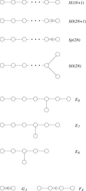
Figure 4.1: Dynkin diagrams for all simple Lie algebras. SU($N$), SO($2N$), and $E_{k}$ are simply laced, meaning that all roots have the same length. For the remaining groups, the arrow points toward the long root(s).

4.1.2 Symmetry breaking and magnetic charges

By an appropriate choice of basis, any element of the Lie algebra — in particular the Higgs vacuum expectation value $\Phi_{0}$ — can be taken to lie in the Cartan subalgebra. We can use this fact to characterize the Higgs vacuum by a vector $\bf h$ defined by

$$\Phi_{0}={\bf h}\cdot{\bf H}\,.$$ (4.1.9)

The generators of the unbroken subgroup are those generators of $G$ that commute with $\Phi_{0}$. These are all the generators of the Cartan subalgebra, together with the ladder operators corresponding to roots orthogonal to $\bf h$. There are two cases to be distinguished. If none of the $\alpha$ are orthogonal to $\bf h$, the unbroken subgroup is the U(1)^r generated by the Cartan subalgebra. If instead there are some roots $\gamma$ with ${\mbox{\boldmath$\gamma$}}\cdot{\bf h}=0$, then these form the root diagram for some semisimple group $K$ of rank $r^{\prime}$, and the unbroken subgroup is $K\times{\rm U(1)}^{r-r^{\prime}}$.

For the time being we will concentrate on the former case, which we will term maximal symmetry breaking (MSB), leaving consideration of the case with a non-Abelian unbroken symmetry to Chap. 6. Because $\Pi_{2}(G/H)=\Pi_{1}[{\rm U(1)}^{r}]=Z^{r}$, the single integer topological charge of the SU(2) case is replaced by an $r$-tuple of integer charges.

To define these charges, we must examine the asymptotic form of the magnetic field. At large distances $B_{i}$ must commute with the Higgs field. Hence, if in some direction $\Phi$ is asymptotically of the form of Eq. (4.1.9), we can choose $B_{i}$ to also lie in the Cartan subalgebra, and can characterize the magnetic charges by a vector $\bf g$ defined by

$$B_{k}=\frac{{\hat{r}}_{k}}{4\pi r^{2}}{\bf g}\cdot{\bf H}\,.$$ (4.1.10)

The generalization of the SU(2) topological charge quantization is the requirement that

$$e^{ie{\bf g}\cdot{\bf H}}=I$$ (4.1.11)

for all representations of $G$ [57, 58]. This is equivalent to requiring that $\bf g$ be a linear combination

$${\bf g}=\frac{4\pi}{e}\sum_{a=1}^{k}n_{a}{\mbox{\boldmath$\beta$}}_{a}^{*}$$ (4.1.12)

of the duals of the simple roots. The integers $n_{a}$ are the desired topological charges.

We noted above that there are many possible ways to choose the simple roots. Each leads to a different set of $n_{a}$, with the various choices being linear combinations of each other. A particularly natural set is specified by requiring that the simple roots all satisfy

$${\mbox{\boldmath$\beta$}}_{a}\cdot{\bf h}>0\,.$$ (4.1.13)

Associated with this set are $r$ fundamental monopole solutions, each of which is a self-dual BPS solution carrying one unit of a single topological charge. Thus, the $a$th fundamental monopole has topological charges

$$n_{b}=\delta_{ab}$$ (4.1.14)

and, by the BPS mass formula of Eq. (3.2.13), has mass

$$m_{a}={4\pi\over e}{\bf h}\cdot{\mbox{\boldmath$\beta$}}^{*}_{a}\,.$$ (4.1.15)

This fundamental monopole can be obtained explicitly by embedding the unit SU(2) solution in the subgroup defined by ${\mbox{\boldmath$\beta$}}_{a}$ via Eq. (4.1.7). If $A^{(s)}_{i}({\bf r};v)$ and $\Phi^{(s)}_{i}({\bf r};v)$ ($s=1,2,3$) are the gauge and scalar fields of the SU(2) monopole with Higgs expectation value $v$, then the $a$th fundamental monopole solution is

$$A_{i} = \sum_{s=1}^{3}A^{(s)}_{i}({\bf r};{\mbox{\boldmath$\beta$}}_{a}\cdot{\bf h})\,t^{s}({\mbox{\boldmath$\beta$}}_{a})$$ (4.1.16)

$$\Phi = \sum_{s=1}^{3}\Phi^{(s)}_{i}({\bf r};{\mbox{\boldmath$\beta$}}_{a}\cdot{\bf h})\,t^{s}({\mbox{\boldmath$\beta$}}_{a})+\left[{\bf h}-({\bf h}\cdot{\mbox{\boldmath$\beta$}}^{*}_{a})\,{\mbox{\boldmath$\beta$}}_{a}\right]\cdot{\bf H}\,\,.$$ (4.1.17)

(The second term in $\Phi$ is needed to give the proper asymptotic value for the scalar field.)

With the aid of Eqs. (4.1.12) and (4.1.15), the energy of a self-dual BPS solution with topological charges $n_{a}$ can be written as a sum of fundamental monopole masses,

$$M=n_{a}m_{a}\,.$$ (4.1.18)

While it may not be obvious that such solutions actually exist for all choices of the $n_{a}$ (an issue that we will address later in this chapter), some higher charge solutions can be written down immediately. Since every root, simple or not, defines an SU(2) subgroup, the embedding construction used to obtain the fundamental monopoles can be carried out for any composite root $\alpha$. The topological charges of the corresponding solution are the coefficients in the expansion

$${\mbox{\boldmath$\alpha$}}^{*}=n_{a}{\mbox{\boldmath$\beta$}}_{a}^{*}\,.$$ (4.1.19)

At first sight, the embedded solutions based on composite roots seem little different than the fundamental monopole solutions. However, there is an essential, although quite surprising, difference. Whereas the fundamental monopoles are unit solitons corresponding to one-particle states, the index theory results that we will obtain in the next section show that the solutions obtained from composite roots are actually multimonopole solutions. They correspond to several fundamental monopoles that happed to be superimposed at the same point, but that can be freely separated.

The ideas of this section can be made a bit more explicit by focussing on the case of SU($N$), which has rank $N-1$. Its Lie algebra can be represented by the set of traceless Hermitian $N\times N$ matrices. The $H_{i}$ can be taken to be the $N-1$ diagonal generators. The $E_{\mbox{\boldmath$\scriptstyle\alpha$}}$ are then the $N(N-1)$ matrices that have a single nonzero element in an off-diagonal position. The Higgs expectation value $\Phi_{0}$ can be taken to be diagonal, with matrix elements

$$s_{1}\leq s_{2}\leq\cdots\leq s_{N}\,.$$ (4.1.20)

If any $k\geq 2$ of the $s_{j}$ are equal, there is an unbroken SU($k$) subgroup. Otherwise, the symmetry breaking is maximal, and the simple roots defined by Eq. (4.1.13) correspond to the matrix elements lying just above the main diagonal. The fundamental monopoles are embedded in $2\times 2$ blocks lying along the diagonal, with the $a$th fundamental monopole lying at the intersections of the $a$th and $(a+1)$th rows and columns and having a mass proportional to $s_{a+1}-s_{a}$. In a direction where the asymptotic Higgs field is diagonal with matrix elements obeying Eq. (4.1.20), the asymptotic magnetic field is

$$B_{k}={1\over 2e}\,\frac{{\hat{r}}_{k}}{r^{2}}\,{\rm diag}\left(-n_{1},n_{1}-n_{2},\dots,n_{N-2}-n_{N-1},n_{N-1}\right)\,.$$ (4.1.21)

Finally, we conclude this section with a brief note about normalizations. It is sometimes convenient to modify the normalization given by Eq. (4.1.1), so that the $H_{i}$ obey

$${\rm Tr\,}(H_{i}H_{j})={c^{2}\over 2}\,\delta_{ij}$$ (4.1.22)

with $c\neq 1$. Under a rescaling of the normalization constant $c$, the roots ${\mbox{\boldmath$\alpha$}}\sim c$, while their duals ${\mbox{\boldmath$\alpha$}}^{*}\sim c^{-1}$. To maintain the correct quantization of the topological charge, $\bf g\sim c^{-1}$.

4.1.3 Generalizing Montonen-Olive duality

At the end of Chap. 3 we discussed the duality conjecture of Montonen and Olive. This conjecture was motivated by the invariance of the BPS spectrum if the transformation $e\leftrightarrow 4\pi/e$ is accompanied by a simultaneous interchange of electric and magnetic charges. We are now in a position to ask how this duality conjecture might be generalized to the case of larger gauge groups.

The first step is to identify the particles to be exchanged by the duality. In the SU(2) theory these are the massive electrically charged gauge boson and its superpartners, on the one hand, and the magnetically charged supermultiplet obtained from the unit monopole and the various possible excitations of the fermion zero modes in its presence. With a larger gauge group, the particle spectrum of the electrically-charged sector is again composed of the gauge bosons that acquire masses through the Higgs mechanism, and their superpartners. On the magnetically charged side, matters are more subtle. The simpest guess is that the dual states should be built upon the classical solutions obtained by using the various roots of the Lie algebra to embed the SU(2) unit monopole. The problem with this is that, as we noted in the previous section, the embedded solution is actually a multimonopole solution if the root $\alpha$ used for the embedding is composite; only embeddings via the simple roots yield one-monopole solutions.

As we will explain in Chap. 9, this difficulty is resolved by the existence of threshold bound states of the appropriate fundamental monopoles. These arise by a rather subtle mechanism involving the fermion fields, and are only possible if the theory has ${\cal N}=4$ supersymmetry. The existence of these bound states has been explicitly demonstrated for the case where the embedding root $\alpha$ is the sum of two simple roots [55, 56]. Because the construction used for this case becomes much more tedious when more than two simple roots are involved, the existence of the bound states for these cases has not been verified, although there seems little doubt that they are present. For the remainder of this discussion, we will simply assume their existence.

The next step is to look more closely at the masses of these particles. The gauge boson associated with the root $\alpha$ has a mass

$$M_{{\mbox{\boldmath$\alpha$}}}=e{\bf h}\cdot{\mbox{\boldmath$\alpha$}}\,.$$ (4.1.23)

This should be compared with the mass

$$m_{{\mbox{\boldmath$\alpha$}}}={4\pi\over e}{\bf h}\cdot{\mbox{\boldmath$\alpha$}}^{*}={4\pi\over e}\,{{\bf h}\cdot{\mbox{\boldmath$\alpha$}}\over{\mbox{\boldmath$\alpha$}}^{2}}$$ (4.1.24)

of the magnetically charged state (whether a fundamental monopole or a threshhold bound state) associated with the same root. The crucial point to note here is the appearance of the root in the former case, but of its dual in the latter.

For gauge groups whose root vectors all have the same length $\mu$ (the so-called “simply laced” groups), the roots and their duals differ by a trivial factor of $\mu^{2}$. All that is necessary to generalize the duality conjecture is to replace the transformation $e\leftrightarrow 4\pi/e$ by $e\leftrightarrow 4\pi/e\mu^{2}$; indeed, the necessity of the additional factor becomes clear as soon as one recalls that the normalization of the gauge coupling depends on the convention that determines the root length.

However, the situation is not so simple if the gauge group has roots of two different lengths, since in this case the roots and their duals are not related by a common rescaling factor. Instead, replacing all of the roots by their duals is equivalent, up to an overall rescaling, to simply interchanging the short and the long roots. It is a remarkable fact [57, 58] that the new set of roots obtained in this fashion is again the root system of a Lie algebra, although not necessarily the original one.

This is easily demonstrated for the rank $N$ algebras SO($2N+1$) and Sp($2N$). Let $e_{i}$, $i=1,2,\dots,N$ be a set of unit vectors in $N$-dimensional Euclidean space. The roots of SO($2N+1$) can then be written as $\pm\sqrt{2}\,e_{i}$ and $(\pm e_{i}\pm e_{j})/\sqrt{2}$ ($i\neq j$), while those of Sp($2N$) can be chosen to be $\pm e_{i}/\sqrt{2}$ and $(\pm e_{i}\pm e_{j})/\sqrt{2}$ ($i\neq j$). Replacing each root of SO($2N+1$) by its dual then simply yields the roots of Sp($2N$), and conversely. The other two non-simply laced Lie algebras, $F_{4}$ and $G_{2}$, are self-dual, up to a rotation; i.e., replacing the roots by their duals yields the initial root system, but rotated. [The same is actually true of the algebras SO(5) and Sp(4), which are identical.]

The generalized Montonen-Olive conjecture can now be stated as follows [59]. Theories with simply laced gauge groups are self-dual under the interchange of electric and magnetic charges and weak and strong coupling. If the gauge group has a Lie algebra that is not simply laced, but is still self-dual, the theory is again self-dual, but with appropriate relabeling of states. In the remaining cases [SO($2N+1$) and Sp($2N$) with $N\geq 3$], the duality maps the gauge theory onto the theory with the dual gauge group.

4.2 Index calculations

In Chap. 2 we noted the existence of four zero modes (in addition to those due to local gauge transformations) about the unit monopole, and related that fact to the existence of a four-dimensional moduli space of solutions. We will now consider the zero modes about BPS solutions of arbitrary charge. In contrast with the previous case, we do not know the form of the unperturbed solution. Also unlike the case of unit charge, the zero modes do not all arise from the action of symmetries on the monopole solution. It is, nevertheless, possible to determine the number of these zero modes [49, 60].

The first step, which we describe in Sec. 4.2.1, is to formulate the problem in terms of a matrix differential operator $\cal D$, and to define a quantity $\cal I$ that counts the normalizable zero modes of $\cal D$. Next, in Sec. 4.2.2, we rewrite the problem in terms of a Dirac equation. This translation from bosonic to fermionic language both simplifies the calculation and illuminates some important properties of the moduli space. The actual evaluation of $\cal I$ is described in Sec. 4.2.3.

4.2.1 Perturbation equations

For the calculations in this section, it will be convenient to adopt a notation where the fields $A_{i}$ and $\Phi$ of the unperturbed solution are written as anti-Hermitian matrices in the adjoint representation of the group, while the perturbations $\delta A_{i}$ and $\delta\Phi$ are written as column vectors. Using this notation, we expand Eq. (3.2.14). Keeping terms linear in the perturbation gives

$$0=D_{i}\delta\Phi-e\Phi\delta A_{i}-\epsilon_{ijk}D_{j}\delta A_{k}$$ (4.2.1)

where

$$D_{i}=\partial_{i}+eA_{i}$$ (4.2.2)

is the covariant derivative with respect to the unperturbed solution.

The solutions of Eq. (4.2.1) include perturbations that are local gauge transformations of the form

$$\delta A_{i}=D_{i}\Lambda\,,\qquad\qquad\delta\Phi=e\Phi\Lambda\,.$$ (4.2.3)

We are not interested in these, and so require that our perturbations be orthogonal to such gauge transformations, in the sense that

$$0 = \int d^{3}x\left[(D_{i}\Lambda)^{\dagger}\delta A_{i}+e(\Phi\Lambda)^{\dagger}\delta\Phi\right]$$ (4.2.4)

$$= -\int d^{3}x\,\Lambda^{\dagger}\left[D_{i}\delta A_{i}+e\Phi\delta\Phi\right]+\int d^{2}S_{i}\,\Lambda^{\dagger}\delta A_{i}\,.$$ (4.2.5)

(The last integral is to be taken over a surface at spatial infinity.) For gauge functions $\Lambda(x)$ that fall off sufficiently rapidly that the surface term vanishes, orthogonality is ensured by imposing the background gauge condition

$$0=D_{i}\,\delta A_{i}+e\Phi\,\delta\Phi\,.$$ (4.2.6)

This does not eliminate all of the gauge modes for which $\Lambda(\infty)$ is nonzero. The surviving modes correspond to global gauge transformations in the unbroken subgroup. These modes are physically significant, as we saw in the analysis of the U(1) phase mode and the related dyons in Sec. 2.4.

Our goal is to count the number of linearly independent solutions of Eqs. (4.2.1) and (4.2.6). These equations can be combined into a single matrix equation

$$0={\cal D}\Psi$$ (4.2.7)

where $\Psi=(\delta A_{1},\delta A_{2},\delta A_{3},\delta\Phi)^{t}$ and

$${\cal D}=\left(\matrix{-e\Phi&D_{3}&-D_{2}&D_{1}\cr-D_{3}&-e\Phi&D_{1}&D_{2}\cr D_{2}&-D_{1}&-e\Phi&D_{3}\cr-D_{1}&-D_{2}&-D_{3}&e\Phi\cr}\right)\,\,.$$ (4.2.8)

The quantity that we want is the number of normalizable zero modes of $\cal D$. These are the same as the normalizable zero modes of ${\cal D}^{\dagger}{\cal D}$, where ${\cal D}^{\dagger}$ is the adjoint of $\cal D$. (Note that ${\cal D}^{\dagger}$ differs from $\cal D$ only in the signs of the diagonal elements.)

Let us define

$${\cal I}=\lim_{M^{2}\to 0}{\cal I}(M^{2})$$ (4.2.9)

where

$${\cal I}(M^{2})={\rm Tr\,}\left({M^{2}\over{\cal D}^{\dagger}{\cal D}+M^{2}}\right)-{\rm Tr\,}\left({M^{2}\over{\cal D}{\cal D}^{\dagger}+M^{2}}\right)$$ (4.2.10)

and ${\rm Tr\,}$ indicates a combined matrix and functional trace. Each normalizable zero mode of ${\cal D}^{\dagger}{\cal D}$ contributes 1 to the right-hand side of Eq. (4.2.10), while each normalizable zero mode of ${\cal D}{\cal D}^{\dagger}$ contributes $-1$. However, by making use of the fact that $A_{i}$ and $\Phi$ obey the Bogomolny equation, it is easy to show that

$${\cal D}{\cal D}^{\dagger}=-D_{j}^{2}-e^{2}\Phi^{2}\,.$$ (4.2.11)

This is a manifestly positive definite operator (remember that $\Phi$ is an anti-Hermitian matrix) and therefore has no normalizable zero modes. It would thus seem that $\cal I$ is precisely the quantity that we want.

There is one potential complication. Because we are dealing with operators that have continuum spectra extending down to zero, we must worry about a possible contribution to $\cal I$ from the continuum. Such a contribution would be of the form

$${\cal I}_{\rm cont}=\lim_{M^{2}\to 0}M^{2}\int{d^{3}k\over(2\pi)^{3}}{1\over k^{2}+M^{2}}\left[\rho_{{\cal D}^{\dagger}{\cal D}}(k^{2})-\rho_{{\cal D}{\cal D}^{\dagger}}(k^{2})\right]$$ (4.2.12)

where $\rho_{\cal O}(k^{2})$ is the density of continuum eigenvalues of the operator $\cal O$. For this to be nonvanishing, the $\rho_{\cal O}(k^{2})$ must be rather singular at $k^{2}=0$.

Singularities of this sort are absent when there is maximal symmetry breaking. This is most easily understood by viewing the theory in a string gauge, where the correspondence between particles and field components is clearest. First, note that the small-$k$ behavior of the densities of states is determined by the large-distance structure of the differential operators. Hence, terms in $\cal D$ and ${\cal D}^{\dagger}$ that fall exponentially with distance can be ignored. The potentially dangerous terms that fall as inverse powers of $r$ can only arise from field components corresponding to the massless gauge and Higgs bosons. Further, the only modes that can have eigenvalues near zero are those with components corresponding to perturbations of these massless fields. Because the unbroken theory is Abelian, the massless fields do not interact with themselves. The long-range terms in $\cal D$ and ${\cal D}^{\dagger}$ therefore have negligible effect on the small-$k$ behavior and cannot give rise to any singularities. Hence, ${\cal I}_{\rm cont}=0$.

If, instead, the unbroken gauge group is non-Abelian, the long-range fields in the unperturbed solution can act on the massless perturbations, and the above arguments no longer apply [61]. We will return to this issue in Sec. 6.1, where we will see that a nonzero continuum contribution to $\cal I$ actually does arise in certain situations.

4.2.2 Connection to Dirac zero modes and supersymmetry

Let us define a $2\times 2$ matrix $\psi$ by

$$\psi=I\delta\Phi+i\sigma_{j}\delta A_{j}\,.$$ (4.2.13)

Equations (4.2.1) and (4.2.6) can then be rewritten as the Dirac-type equation [62]

$$0=(-i\sigma_{j}D_{j}+e\Phi)\psi\equiv{\cal D}_{f}\psi\,.$$ (4.2.14)

Note, however, that when Eq. (4.2.13) is inverted to give $\delta A_{j}$ and $\delta\Phi$ in terms of $\psi$, the bosonic perturbations obtained from $i\psi$ are linearly independent of those obtained from $\psi$. The number of normalizable zero modes of $\cal D$ is thus twice the number of normalizable zero modes of the Dirac operator ${\cal D}_{f}$. Hence, if ${\cal I}_{f}$ is defined in the same manner as $\cal I$, but with ${\cal D}$ replaced by ${\cal D}_{f}$, the two quantities will be related by

$${\cal I}=2{\cal I}_{f}\,.$$ (4.2.15)

This shows that the number of bosonic zero modes must be even. In fact, an even stronger result holds. If $\psi$ is a solution to Eq. (4.2.14), then so is $\psi U$, where $U$ is any unitary $2\times 2$ matrix. By this means a second linearly independent $\psi$ can be constructed from the first. Together, this complex doublet of Dirac modes implies a set of four linearly independent bosonic zero modes. To make this explicit, let us use a four-dimensional Euclidean notation, similar to that introduced in Sec. 2.5, where $\delta\Phi=\delta A_{4}$. If $\delta A_{a}$ is the bosonic zero mode corresponding to the Dirac solution $\psi$, then the zero mode corresponding to $\psi^{\prime}=i\psi\sigma_{r}$ has components

$$(\delta A)^{\prime}_{a}=-\bar{\eta}^{r}_{ab}\delta A_{b}$$ (4.2.16)

where the anti-self-dual tensor $\bar{\eta}^{r}_{ab}$ and its self-dual counterpart $\eta^{r}_{ab}$ (with $r=1,\,2,\,3$) are defined by $\eta^{r}_{ij}=\bar{\eta}^{r}_{ij}=\epsilon_{rij}$, $\eta^{r}_{a4}=-\bar{\eta}^{r}_{a4}=\delta_{ra}$. Because of the antisymmetry of the $\bar{\eta}^{r}_{ab}$, $\delta A^{\prime}$ is orthogonal to $\delta A$ at each point in space.

The zero modes form a basis for the tangent space at a given point on the moduli space. We thus have three maps $J^{(r)}$ of this tangent space onto itself, with

$${J^{(r)}}_{m}{}^{n}\,\delta_{n}A_{a}=-\bar{\eta}^{r}_{ab}\delta_{m}A_{b}\,.$$ (4.2.17)

These obey the quaternionic algebra

$$J^{(r)}J^{(s)}=-\delta^{rs}+\epsilon^{rst}J^{(t)}$$ (4.2.18)

and thus define a local quaternionic structure on the moduli space. In Sec. 5.1 we will obtain an even stronger result, that the moduli space is hyper-Kähler.

The existence of these multiplets of zero modes, and of the hyper-Kähler structure that follows from them, can be understood in terms of supersymmetry. We have seen that by the addition of appropriate fermion and scalar fields the Lagrangian can be extended to that of ${\cal N}=4$ SYM theory, and that this is the most natural setting for the Bogomolny equation. Because the BPS solution breaks only half of the supersymmetry, the zero modes about any solution must fall into complete multiplets under the unbroken ${\cal N}=2$ supersymmetry. The smallest possible multiplet has four real bosonic and four real fermionic components, with the fermionic components transforming as a complex doublet under the SU(2) R-symmetry.

In fact, there are always four bosonic zero modes that can be obtained directly from a supersymmetry transformation. We saw in Sec. 3.3 that half of the supersymmetry in the ${\cal N}=2$ or ${\cal N}=4$ SYM theories is preserved by the BPS solutions. Acting on these solutions with the generators of the broken supersymmetry produces Dirac zero modes. In particular, by examining Eqs. (3.3.15) – (3.3.22), with $\alpha=0$ and $\zeta_{1}=i\gamma^{5}\gamma^{0}\zeta_{2}$, we see that

$$\psi=i{\mbox{\boldmath$\sigma$}}\cdot{\bf B}$$ (4.2.19)

should be a solution of Eq. (4.2.14), as can be easily verified. Guided by Eq. (4.2.13), we immediately read off the bosonic zero mode

$$\delta A_{i}=B_{i}\,,\qquad\delta\Phi=0$$ (4.2.20)

that corresponds to a global U(1) phase rotation. Acting on this mode with the three $J^{(p)}$ yields the three translation zero modes

$$\delta_{p}A_{i}=F_{pi}\,,\qquad\delta\Phi=D_{p}\Phi\,.$$ (4.2.21)

[These differ from the naive form of the translation zero mode, $\delta_{p}A_{i}=\partial_{p}A_{i}$ and $\delta_{p}\Phi=\partial_{p}\Phi$, by a local gauge transformation with gauge function $\Lambda=-A_{p}$, and thereby satisfy the background gauge condition, Eq. (4.2.6).]

4.2.3 Evaluation of ${\cal I}$

Returning to our calculation, let us define a set of Euclidean Dirac matrices

$$\Gamma_{k}=\left(\matrix{0&-i\sigma_{k}\cr i\sigma_{k}&0}\right)\,,\qquad\Gamma_{4}=\left(\matrix{0&I\cr I&0}\right)$$ (4.2.22)

obeying

$$\{\Gamma_{a},\Gamma_{b}\}=2\delta_{ab}\,,$$ (4.2.23)

as well as

$$\Gamma_{5}=\Gamma_{1}\Gamma_{2}\Gamma_{3}\Gamma_{4}=\left(\matrix{I&0\cr 0&-I}\right)\,.$$ (4.2.24)

As in the preceding section, it will sometimes be convenient to use the four-dimensional notation in which $A_{4}=\Phi$, $F_{a4}=D_{a}\Phi$, and (because we are using adjoint representation matrices for the unperturbed fields in this section) $D_{4}=e\Phi$. However, we will at times need to switch back to the three–dimensional notation. To distinguish between the two, we will let indices $a,b,\dots$ range from 1 to 4, while $i,j,\dots$ will range from 1 to 3.

With this notation,

$$\Gamma\cdot D=\Gamma_{a}D_{a}=\left(\matrix{0&{\cal D}_{f}\cr-{\cal D}_{f}^{\dagger}&0}\right)$$ (4.2.25)

and

$${\cal I}_{f}(M^{2}) = -{\rm Tr\,}\Gamma_{5}{M^{2}\over-(\Gamma\cdot D)^{2}+M^{2}}$$ (4.2.26)

$$= -\int d^{3}x\,{\rm tr}\left\langle x\left|\Gamma_{5}{M^{2}\over-(\Gamma\cdot D)^{2}+M^{2}}\right|x\right\rangle$$ (4.2.29)

$$= -\int d^{3}x\,{\rm tr}\left\langle x\left|\Gamma_{5}{M\left[-(\Gamma\cdot D)+M\right]\over-(\Gamma\cdot D)^{2}+M^{2}}\right|x\right\rangle$$ (4.2.32)

$$= -\int d^{3}x\,{\rm tr}\left\langle x\left|\Gamma_{5}{M\over(\Gamma\cdot D)+M}\right|x\right\rangle$$ (4.2.35)

where ${\rm tr}$ indicates a trace only over Dirac and group indices. (To obtain the third equality, one must use the cyclic property of the trace and the fact that $\Gamma_{5}$ anticommutes with an odd number of $\Gamma$-matrices.)

The trick to the evaluation of $\cal I$ is to show that the integrand on the right-hand side is a total divergence. This allows ${\cal I}_{f}(M^{2})$ to be written as a surface integral at spatial infinity that depends only on the asymptotic behavior of the fields. To this end, we define a nonlocal current

$$J_{i}(x,y)={\rm tr}\left\langle x\left|\Gamma_{5}\Gamma_{i}{1\over(\Gamma\cdot D)+M}\right|y\right\rangle\,.$$ (4.2.36)

Using the identities

$$\delta(x-y) = \left[\Gamma_{i}{\partial\over\partial x_{i}}+e\Gamma\cdot A+M\right]\left\langle x\left|{1\over(\Gamma\cdot D)+M}\right|y\right\rangle$$ (4.2.37)

$$= \left\langle x\left|{1\over(\Gamma\cdot D)+M}\right|y\right\rangle\left[-\Gamma_{i}{\overleftarrow{\partial}\over\partial x_{i}}+e\Gamma\cdot A+M\right]$$ (4.2.39)

and the cyclic property of the trace, we find that

$$\left({\partial\over\partial x_{i}}+{\partial\over\partial y_{i}}\right)J_{i}(x,y) = -{\rm tr}\left[2M-e\Gamma\cdot A(x)+e\Gamma\cdot A(y)\right]\left\langle x\left|\Gamma_{5}{1\over(\Gamma\cdot D)+M}\right|y\right\rangle.$$ (4.2.40)

The manipulations here are analogous to those used in the calculation of the divergence of the four-dimensional axial current. In four dimensions, there are short-distance singularities as $y$ approaches $x$ that produce an anomaly. In three dimensions these singularities are weaker and there is no anomaly. We can therefore set $x=y$ in Eq. (LABEL:splitcurrentdiv) and, by comparing with Eq. (4.2.35), obtain

$${\cal I}_{f}(M^{2}) = {1\over 2}\int d^{3}x\,\partial_{i}J_{i}(x,x)$$ (4.2.43)

$$= {1\over 2}\lim_{R\to\infty}\int_{R}dS_{i}\,J_{i}(x,x)$$ (4.2.45)

where the surface of integration in the last line is a sphere of radius $R$.

We now rewrite $J_{i}(x,x)$ as

$$J_{i}(x,x)=-{\rm tr}\left\langle x\left|\Gamma_{5}\Gamma_{i}\,(\Gamma\cdot D)\,{1\over-(\Gamma\cdot D)^{2}+M^{2}}\right|x\right\rangle\,.$$ (4.2.46)

Because

$$-(\Gamma\cdot D)^{2}+M^{2}=-D_{j}^{2}-e^{2}\Phi^{2}+M^{2}-{e\over 4}[\Gamma_{a},\Gamma_{b}]F_{ab}$$ (4.2.47)

the last factor in Eq. (4.2.46) can be expanded as

$${1\over-(\Gamma\cdot D)^{2}+M^{2}} = {1\over-D_{j}^{2}-e^{2}\Phi^{2}+M^{2}}$$ (4.2.48)

$$+ \,{1\over-D_{j}^{2}-e^{2}\Phi^{2}+M^{2}}\left({e\over 4}[\Gamma_{a},\Gamma_{b}]F_{ab}\right){1\over-D_{j}^{2}-e^{2}\Phi^{2}+M^{2}}$$ (4.2.51)

$$+ \,\cdots\,.$$ (4.2.54)

When this expansion is inserted into Eq. (4.2.46), the contribution from the first term vanishes after the trace over Dirac indices is taken, while the $1/x^{2}$ falloff of $F_{ab}$ implies that the terms represented by the ellipsis do not contribute to the surface integral. To evaluate the remaining term, we write

$$F_{ij}=\epsilon_{ijk}F_{k4}=\epsilon_{ijk}B_{k}=\epsilon_{ijk}{\hat{x}_{k}\over 4\pi\,x^{2}}Q+O(1/x^{3})$$ (4.2.55)

where $Q$ is an element of the Lie algebra specifying the magnetic charge. Inserting this into Eq. (4.2.46) and performing the Dirac trace leads to

$$\hat{x}_{i}J_{i}(x,x) = -{e^{2}\over\pi\,x^{2}}\,{\rm tr}\left\langle x\left|\Phi{1\over-\nabla_{j}^{2}-e^{2}\Phi^{2}+M^{2}}Q{1\over-\nabla_{j}^{2}-e^{2}\Phi^{2}+M^{2}}\right|x\right\rangle$$ (4.2.58)

$$+O(1/x^{3})$$

where now ${\rm tr}$ indicates a trace only over group indices.

By an appropriate gauge transformation, we can put the asymptotic Higgs and magnetic fields into forms corresponding to those in Eqs. (4.1.9) and (4.1.10). Keeping track of the sign changes that arise because the $H_{i}$ are Hermitian, we obtain

$$\hat{x}_{i}J_{i}(x,x)={e^{2}\over\pi\,x^{2}}\,{\rm tr}\left\langle x\left|{({\bf h}\cdot{\bf H})({\bf g}\cdot{\bf H})\over\left[-\nabla_{j}^{2}+e^{2}({\bf h}\cdot{\bf H})^{2}+M^{2}\right]^{2}}\right|x\right\rangle+O(1/x^{3})\,.$$ (4.2.59)

In the adjoint representation the matrix elements of the generators are given by the structure constants. In particular, the matrix elements of the $H_{i}$ are determined by the roots. The matrix trace in the above equation thus leads to a sum over roots, and

$$\hat{x}_{i}J_{i}(x,x)={e^{2}\over\pi\,x^{2}}\,\sum_{\mbox{\boldmath$\scriptstyle\alpha$}}\left\langle x\left|{({\bf h}\cdot{\mbox{\boldmath$\alpha$}})({\bf g}\cdot{\mbox{\boldmath$\alpha$}})\over\left[-\nabla_{j}^{2}+e^{2}({\bf h}\cdot{\mbox{\boldmath$\alpha$}})^{2}+M^{2}\right]^{2}}\right|x\right\rangle+O(1/x^{3})\,.$$ (4.2.60)

Using the identity

$$\left\langle x\left|{1\over\left(-\nabla_{j}^{2}+\mu^{2}\right)^{2}}\right|x\right\rangle=\int{d^{3}k\over(2\pi)^{3}}\,{1\over(k^{2}+\mu^{2})^{2}}={1\over 8\pi\mu}$$ (4.2.61)

then gives

$$\hat{x}_{i}J_{i}(x,x)={e^{2}\over 8\pi^{2}\,x^{2}}\,\sum_{\mbox{\boldmath$\scriptstyle\alpha$}}{({\bf h}\cdot{\mbox{\boldmath$\alpha$}})({\bf g}\cdot{\mbox{\boldmath$\alpha$}})\over\left[e^{2}({\bf h}\cdot{\mbox{\boldmath$\alpha$}})^{2}+M^{2}\right]^{1/2}}+O(1/x^{3})\,.$$ (4.2.62)

The contributions to the sum from the positive and negative roots are clearly equal, so we can insert a factor of two and restrict the sum to the positive roots. Then substituting this last equation into Eq. (4.2.45), we obtain

$${\cal I}_{f}(M^{2})={e^{2}\over 2\pi}\,{\sum_{\mbox{\boldmath$\scriptstyle\alpha$}}}^{\prime}{({\bf h}\cdot{\mbox{\boldmath$\alpha$}})({\bf g}\cdot{\mbox{\boldmath$\alpha$}})\over\left[e^{2}({\bf h}\cdot{\mbox{\boldmath$\alpha$}})^{2}+M^{2}\right]^{1/2}}\,.$$ (4.2.63)

Taking the limit $M^{2}\rightarrow 0$, using the fact that all positive roots satisfy ${\mbox{\boldmath$\alpha$}}\cdot{\bf h}>0$, and inserting Eq. (4.1.12), we then find

$${\cal I}_{f} = {e\over 2\pi}\,{\sum_{\mbox{\boldmath$\scriptstyle\alpha$}}}^{\prime}{\bf g}\cdot{\mbox{\boldmath$\alpha$}}$$ (4.2.64)

$$= 2\,\sum_{a}n_{a}\,{\sum_{\mbox{\boldmath$\scriptstyle\alpha$}}}^{\prime}{{\mbox{\boldmath$\beta$}}}_{a}^{*}\cdot{\mbox{\boldmath$\alpha$}}$$ (4.2.65)

where the prime indicates that the sum is only over the positive roots. We now make use of the fact that if ${{\mbox{\boldmath$\beta$}}}_{a}$ is any simple root, and ${\mbox{\boldmath$\alpha$}}\neq{{\mbox{\boldmath$\beta$}}}_{a}$ is a positive root, then reflection in a hyperplane orthogonal to ${{\mbox{\boldmath$\beta$}}}_{a}$ gives another positive root ${{\mbox{\boldmath$\alpha$}}}^{\prime}$ with ${{\mbox{\boldmath$\alpha$}}}^{\prime}\cdot{{\mbox{\boldmath$\beta$}}}_{a}=-{\mbox{\boldmath$\alpha$}}\cdot{{\mbox{\boldmath$\beta$}}}_{a}$. Hence, all the terms in the sum over $\alpha$ cancel pairwise, except for the one with ${\mbox{\boldmath$\alpha$}}={{\mbox{\boldmath$\beta$}}}_{a}$, and we have

$${\cal I}_{f}=2\sum_{a}n_{a}\,.$$ (4.2.66)

Finally, the quantity that we want is

$${\cal I}=2{\cal I}_{f}=4\sum_{a}n_{a}\,.$$ (4.2.67)

Equation (4.2.67) tells us that the SU(2) solutions with $n$ units of magnetic charge lie on a $4n$-dimensional moduli space. The natural interpretation is that there are four moduli for each of $n$ independent monopoles. One would expect three of these to specify the position of the monopole. The fourth modulus should be analogous to the fourth zero mode of the unit monopole, which is associated with a global U(1) phase. It is perhaps most easily understood by considering its conjugate momentum. For the unit monopole, this is the electric charge divided by $e$; for solutions with higher charge, excitation of these “U(1)-phase modes” leads to independent electric charges on each of the $n$ component monopoles.

The story is very much the same with larger gauge groups. The fundamental monopoles are obtained by embeddings of the SU(2), and they have only the four position and U(1) modes inherited from that solution. All solutions with higher charge live on higher-dimensional moduli spaces, and are thus naturally understood as multimonopole solutions.

4.3 General remarks on higher charge solutions

The BPS mass formula suggests the possibility of static multimonopole solutions, with the Higgs scalar field mediating an attractive force that exactly cancels the magnetic repulsion between the monopoles. Further, the index theory calculations of the previous section show that the number of parameters entering solutions with higher magnetic charge — if any such solutions exist — is just what might be expected for a collection of noninteracting static monopoles.

While suggestive, neither of these considerations actually establishes that multimonopole solutions exist. However, an existence proof has been given by Taubes [63]. In the context of the SU(2) theory, he showed that there is a finite distance $R$ such that, given arbitrary points ${\bf r}_{1},{\bf r}_{2}\dots,{\bf r}_{N}$ with all $|{\bf r}_{i}-{\bf r}_{j}|>R$, there is a magnetic charge $N$ solution with zeroes of the Higgs field at the given locations.

In the next section we will describe a construction for obtaining these higher charge solutions. Before doing so, we present here some general remarks concerning the nature of these solutions. While we will focus on SU(2) solutions, similar considerations apply with larger gauge groups. We start by considering solutions with $N$ monopoles whose mutual separations are all large compared to the monopole core radius. There are $N$ zeroes of the Higgs field, with a monopole core surrounding each zero and the massive fields falling exponentially outside these cores. These solutions are in a sense both rather complex and yet quite simple.

The complexity becomes evident as soon as one considers the twisting of the Higgs field. In any nonsingular gauge the Higgs field orientation in the neighborhood of each individual monopole must look like that for a singly-charged monopole. However, these Higgs fields must join up at large distances to give a configuration with winding number $N$. The analytic expression for such a configuration cannot be simple.

At the same time, there is an underlying simplicity arising from the fact that, apart from the exponentially small massive fields, the physical fields outside the cores are purely Abelian. These obey linear field equations, and so it should be possible to obtain approximate solutions by superposition. This is most easily done by working in a gauge with uniform Higgs field direction, $\Phi=(0,0,\varphi)$, and defining electromagnetic and massive vector fields ${\cal A}_{\mu}$ and $W_{\mu}$ as in Eq. (2.2.9). In this gauge there is a Dirac string originating at each of the zeros of the Higgs field and running off to spatial infinity. The specific paths of the strings are gauge-dependent; let us assume that they are chosen to avoid all monopole cores except the one in which they originate.

For a single monopole centered at the origin, the electromagnetic field in this gauge is ${\cal A}_{j}({\bf r})=A_{j}^{\rm Dirac}({\bf r})$. The Higgs field can be written as

$$\varphi({\bf r}-{\bf x}^{(a)})=v+\tilde{\varphi}({\bf r};v)\,.$$ (4.3.1)

For $|{\bf r}|\gg M_{W}^{-1}$,

$$\tilde{\varphi}({\bf r};v)=-{1\over er}+O(e^{-evr})$$ (4.3.2)

and the massive vector field $W_{j}({\bf r};v)$ is exponentially small.

Now consider a solution for which the Higgs field has zeros at ${\bf x}^{(a)}$, with $a=1,2,\dots,N$. The linearity of the Abelian theory implies that outside the $n$ core regions

$${\cal A}_{j}({\bf r}) = \sum_{a=1}^{N}A_{j}^{\rm Dirac}({\bf r}-{\bf x}^{(a)})+\cdots$$ (4.3.3)

$$\varphi({\bf r}) = v-\sum_{a=1}^{N}{1\over e|{\bf r}-{\bf x}^{(a)}|}+\cdots$$ (4.3.5)

where the ellipsis represents terms that, like the $W_{j}$ field itself, fall exponentially with distance from the cores.

The fields inside the core regions are similar to those for a single monopole, but with a few notable differences. First, the scalar field tails of the other monopoles reduce the Higgs expectation value seen in the $a$th core from $v$ to

$$v_{\rm eff}^{a}=v-\sum_{b\neq a}{1\over e|{\bf x}^{(a)}-{\bf x}^{(b)}|}+O(e^{-evr_{\rm min}})\,.$$ (4.3.6)

This produces an increase in the core radius, and implies that the Higgs and W fields inside this core are approximately

$$\varphi({\bf r}) \approx v_{\rm eff}+\tilde{\varphi}({\bf r}-{\bf x}^{(a)};v_{\rm eff}^{a})$$ (4.3.7)

$$W_{j}({\bf r}) \approx W_{j}({\bf r}-{\bf x}^{(a)};v_{\rm eff}^{a})\,.$$ (4.3.9)

Because the massive fields fall exponentially with distance, they have negligible effects on the interactions between the monopoles. However, they can have a curious effect on the symmetry of the solutions, with interesting physical consequences. This can be seen most clearly by considering a solution containing two monopoles, one centered at $(0,0,-R)$ and one at $(0,0,R)$, with the Dirac string of the first (second) chosen to run along the $z$-axis from the monopole to $z=-\infty$ ($z=\infty$). Since a single monopole is spherically symmetric, it would be natural to expect that this solution would be axially symmetric under rotations about the $z$-axis.

Let us examine this in more detail. If only the first monopole were present, its Higgs and electromagnetic fields would be invariant under rotation by an angle $\alpha$ about the $z$-axis. Its $W$ field would also be invariant if this rotation were accompanied by a global U(1) gauge transformation with gauge function $\Lambda=e^{-i\alpha}$. Similarly, if only the second monopole were present, it would be invariant under the same rotation, except that the change in direction of the Dirac string would require that $\Lambda=e^{i\alpha}$.

The mismatch between the two gauge transformations means that, despite naive expectations, the solution cannot be axially symmetric. A gauge invariant measure of this is given by the scalar product ${\bf W_{(1)}^{*}}\cdot{\bf W}_{(2)}$, where ${\bf W}_{(a)}$ denotes the field due to the $a$th monopole; this is $O(e^{-evR})$.

One consequence of this breaking of axial symmetry is that the spectrum of fluctuations about the solution must include a zero mode corresponding to spatial rotation about the $z$-axis. A time-dependent excitation of this mode gives a solution with nonzero angular momentum oriented along the axis joining the two monopoles. This can be understood by noting that, because of the mismatch in $\Lambda$’s noted above, this rotation also corresponds to a shift in the relative U(1) phase between the monopoles. When done in a time-dependent fashion, this turns the monopoles into a pair of dyons with equal and opposite electric charges. The angular momentum is just the usual charge-monopole angular momentum, which for a pair of dyons with electric and magnetic charges $q_{j}$ and $g_{j}$ points toward dyon 1 and has a magnitude $g_{1}q_{2}-g_{2}q_{1}$.

In contrast to the case of widely separated monopoles, where the general properties of the solutions could have been anticipated, some surprising features arise when several monopoles are brought close together. We will just note a few examples:

1) When two monopoles are brought together [64, 65, 66, 71], the axial symmetry, whose curious absence we have noted, actually emerges when the two zeros of the Higgs field coincide. The profiles of the energy density and of the Higgs field have a toroidal shape.

2) There is a solution with tetrahedral symmetry [73, 74], with the energy density contours looking like tetrahedra with holes in the centers of each face. Although the Higgs field has a zero at each vertex of the tetrahedron, there is also an antizero (i.e., a zero with opposite winding) at the center. Thus, this is actually a three-monopole solution, illustrating quite dramatically that the zeroes of the Higgs field are not always the same as the monopole positions [75].

3) Solutions corresponding to the other Platonic solids, but again with nonintuitive charges, have been found. There is a cubic $N=4$ solution [73, 74] for which the Higgs field has a four-fold zero at the center and no other zeros [76], an $N=5$ octahedral solution [77] with zeros at the vertices and an antizero at the center [76], an $N=7$ dodecahedral solution [77] with a seven-fold zero at the center [76], and an $N=11$ icosahedral solution [78].

One feature that cannot emerge is spherical symmetry. Not only are there no spherically symmetric SU(2) solutions with $N\geq 2$, there are not even any finite energy configurations with spherical symmetry. This result was first obtained by a detailed analysis of the behavior of gauge fields under rotations, including the effects of the possible compensating gauge transformations [79]. However, a much simpler proof can be obtained by considering the properties of generalized spherical harmonics. This analysis is best done in the string gauge used above, with a uniform SU(2) orientation for the Higgs field, and electromagnetic and massive gauge fields ${\cal A}_{\mu}$ and $W_{\mu}$. Each of these fields can be expanded in spherical harmonics, with the coefficients being functions only of $r$. A spherically symmetric configuration is one that contains only harmonics with total angular momentum quantum number $J=0$.

The spin and charge of a field determine what type of harmonics are appropriate for its expansion. A neutral scalar field can be expanded in terms of the $Y_{LM}$, the eigenfunctions of the orbital angular momentum ${\bf L}={\bf r}\times{\bf p}$. For a charged scalar field one must use the monopole spherical harmonics [80, 81] that take into account the extra charge-monopole angular momentum; because the latter contribution is orthogonal to the usual orbital angular momentum, it places a lower bound on $J$ and implies that the harmonics for a monopole with $q$ units of charge have $J\geq q$. The additional spin angular momentum of a charged vector field, such as $W_{j}$, leads to vector monopole spherical harmonics [82, 83]. These all have $J\geq q-1$, so $W_{j}$ would vanish identically in any spherically symmetric configuration with multiple magnetic charge. This would leave only the the Higgs and electromagnetic fields, giving an essentially U(1) configuration that has infinite energy because of the singularity of the Coulomb field at the origin.

4.4 The Atiyah-Drinfeld-Hitchin-Manin-Nahm construction

Several methods for constructing multimonopole solutions have been developed, including ones using twistor methods [64, 90, 91], Bäcklund transformations [92, 93, 94, 95], and rational maps [96, 97, 98, 99]. However, the method due to Nahm [50, 51, 52, 53] has proven to be the most fruitful. It is readily extended from SU(2) to the other classical groups [102], and also has a natural string theoretic interpretation in terms of D-branes [103].

Nahm’s approach is based on the observation that the monopole solutions of the Bogomolny equation can be viewed as dimensionally reduced analogues of the instanton solutions of the self-dual Yang-Mills equation. For the latter, the Atiyah-Drinfeld-Hitchin-Manin (ADHM) construction [104] gives an equivalence between the solutions of the nonlinear self-duality differential equations in four variables and a set of algebraic matrix equations. From a solution of these matrix equations, an instanton solution can be obtained by solving linear equations.

Nahm generalized this construction to the monopole problem. Instead of an equivalence between differential equations in four variables and a set of purely algebraic equations, this Atiyah-Drinfeld-Hitchin-Manin-Nahm (ADHMN) construction gives an equivalence between the Bogomolny equation in three variables and the Nahm equation, which is a nonlinear differential equation in one variable [105]. The counterparts of the ADHM matrices are matrix functions $T_{\mu}(s)$ ($\mu=0,1,2,3$), known as the Nahm data. [We will see that it is always possible to eliminate $T_{0}(s)$. This is usually done, yielding the more familiar form of the construction in terms of the three $T_{j}(s)$.]

We begin our discussion in Sec. 4.4.1 by presenting, without proof, the prescription for constructing a $k$-monopole solution in the SU(2) theory. Then, in Sec. 4.4.2, we describe some gauge freedoms associated with this construction, and also describe how the symmetries of spacetime are reflected in the Nahm data. In Sec. 4.4.3 we show that the fields obtained by the construction are indeed self-dual; the argument is quite parallel to that for the ADHM construction. We also verify here that the solutions have the correct magnetic charge and that they lie in SU(2). Next, in Sec. 4.4.4, we demonstrate the completeness of the construction by showing that any solution of the Bogomolny equation yields a solution of the Nahm equation. Finally, the extension to other classical groups is described in Sec. 4.4.5.

In order to simplify the equations, we will set the gauge coupling $e$ to unity throughout this section. The factors of $e$ can be easily restored by simple rescalings.

4.4.1 The construction of SU(2) multimonopole solutions

The ADHMN construction of a BPS SU(2) solution with $k$ units of magnetic charge can be viewed as a three-step process:

1) Solving for the Nahm data

The first step is to find a quartet of Hermitian $k\times k$ matrices $T_{\mu}(s)$ that satisfy the Nahm equation,

$$0={dT_{i}\over ds}+i[T_{0},T_{i}]+{i\over 2}\epsilon_{ijk}[T_{j},T_{k}]\,,$$ (4.4.1)

where the indices $i$, $j$, and $k$ run from 1 to 3, and the auxiliary variable $s$ lies in the range $-v/2\leq s\leq v/2$, with $v$ being the Higgs vacuum expectation value. For $k=1$, the $T_{i}(s)$ are clearly constants. For $k>1$, we impose the condition that the $T_{i}(s)$ have poles at the boundaries of the form

$$T_{i}(s)=-\,{L_{i}^{\pm}\over s\mp v/2}+O(1)\,.$$ (4.4.2)

The Nahm equation implies that the $L_{i}^{\pm}$ form $k$-dimensional representations of the SU(2) Lie algebra,

$$[L^{\pm}_{i},L^{\pm}_{j}]=i\epsilon_{ijk}L^{\pm}_{k}\,.$$ (4.4.3)

The final boundary condition is that these representations be irreducible; i.e., they must be equivalent to the angular momentum $(k-1)/2$ representation of SU(2). There are no boundary conditions on $T_{0}$.

2) The construction equation

The next step is to define a linear operator

$$\Delta(s)={d\over ds}+iT_{0}(s)\otimes{\rm I_{2}}-T_{i}(s)\otimes\sigma_{i}+r_{i}{\rm I_{k}}\otimes\sigma_{i}$$ (4.4.4)

and to solve the construction equation

$$0=\Delta^{\dagger}(s)\,w(s,{\bf r})=\left[-{d\over ds}-iT_{0}\otimes{\rm I_{2}}-T_{i}\otimes\sigma_{i}+r_{i}{\rm I_{k}}\otimes\sigma_{i}\right]w(s,{\bf r})$$ (4.4.5)

where $w(s,{\bf r})$ is a $2k$-component vector. (We will usually suppress the indices denoting the components of $w$.)

We are only interested in the normalizable solutions of this equation. We denote by $w_{a}$ a complete linearly independent set of such solutions, and require that they obey the orthonormality condition

$$\delta_{ab}=\int_{-v/2}^{v/2}ds\,w_{a}^{\dagger}(s,{\bf r})w_{b}(s,{\bf r})\,.$$ (4.4.6)

3) Obtaining the spacetime fields

We assert now, and prove below in Sec. 4.4.3, that there are only two normalizable $w_{a}(s,{\bf r})$. The spacetime fields are obtained as $2\times 2$ matrices from these by the equations

$$\Phi^{ab}({\bf r})=\int_{-v/2}^{v/2}ds\,s\,w_{a}^{\dagger}(s,{\bf r})w_{b}(s,{\bf r})$$ (4.4.7)

and

$$A_{j}^{ab}({\bf r})=-i\int_{-v/2}^{v/2}ds\,w_{a}^{\dagger}(s,{\bf r})\partial_{j}w_{b}(s,{\bf r})\,.$$ (4.4.8)

4.4.2 Gauge invariances and symmetries

Every set of Nahm data satisfying the Nahm equation and boundary conditions yields a self-dual spacetime solution. Furthermore, every $\Phi({\bf r})$ and $A_{i}({\bf r})$ obeying the Bogomolny equation can be obtained in this fashion. However, because of the existence of gauge freedom on both sides, the correspondence between Nahm solutions and Bogomolny solutions is not one-to-one.

The usual spacetime gauge transformations correspond to changes in the basis of the solutions of the construction equation,

$$w_{a}(s,{\bf r})\rightarrow w_{a}^{\prime}(s,{\bf r})=w_{b}(s,{\bf r})\,U_{ba}({\bf r})$$ (4.4.9)

with the SU(2) matrix $U({\bf r})$ being the usual spacetime gauge function.

The corresponding gauge symmetry on the Nahm side is an SU($k$) gauge action that preserves the Nahm equation. It takes the form

$$T_{j}(s) \rightarrow T^{\prime}_{j}(s)=g(s)\,T_{j}(s)\,g^{-1}(s)$$ (4.4.10)

$$T_{0}(s) \rightarrow T^{\prime}_{0}(s)=g(s)\,T_{0}(s)\,g^{-1}(s)+i\,{dg(s)\over ds}\,g^{-1}(s)$$ (4.4.11)

where $g(s)$ is an element of SU($k$). If $w(s,{\bf r})$ is a solution of the construction equation defined by the $T_{\mu}$, then

$$w^{\prime}(s,{\bf r})=g(s)\otimes{\rm I}_{2}\,w(s,{\bf r})$$ (4.4.12)

is a solution of the construction equation defined by the $T^{\prime}_{\mu}$. Referring to Eqs. (4.4.7) and (4.4.8), one then sees that, just as the spacetime gauge transformation has no effect on the $T_{\mu}(s)$, this SU($k$) action leaves $\Phi({\bf r})$ and $A_{j}({\bf r})$ unchanged.

By exploiting this SU($k$) gauge action, it is always possible to transform away any nonzero $T_{0}(s)$. We will usually assume that this has been done, and will write the Nahm equation as

$${dT_{i}\over ds}={i\over 2}\epsilon_{ijk}[T_{j},T_{k}]$$ (4.4.13)

and the construction equation as

$$0=\left[-{d\over ds}-T_{i}\otimes\sigma_{i}+r_{i}{\rm I}_{k}\otimes\sigma_{i}\right]w(s,{\bf r})\,.$$ (4.4.14)

In addition to these gauge actions, there are also transformations on the Nahm data that reflect the symmetries of spacetime. If $T_{i}(s)$ is a solution of the Nahm equation, then so is

$$T^{\prime}_{i}(s)=T_{i}(s)+D_{i}{\rm I}_{k}\,.$$ (4.4.15)

Referring to the construction equation, we see that the $T^{\prime}_{i}(s)$ generate a solution that is translated in physical space by a displacement $\bf D$.

Similarly, if $R_{ij}$ is an $s$-independent SO(3) matrix, the replacement of $T_{i}(s)$ by

$$T^{\prime}_{i}(s)=R_{ij}\,T_{j}(s)$$ (4.4.16)

corresponds to a rotation of the spatial coordinates in the construction equation, and thus to a rotation of the solution in physical space.

4.4.3 Verification of the construction

We now show that the fields obtained by the ADHMN construction have the desired properties. Thus, we must show that they are self-dual, i.e., that they satisfy the Bogomolny equation (3.2.14); that they lie in SU(2); and that they have $k$ units of magnetic charge.

1) Proof of self-duality

To verify the self-duality of the fields, we separately calculate $B_{i}$ and $D_{i}\Phi$ and show that the two are equal. The approach described here [105] closely follows that used in Ref. [106] to demonstrate the self-duality of the instanton solutions obtained by the ADHM construction. For the sake of clarity, we will not explicitly show the dependence on the spatial position $\bf r$, although we will have to make use of the spatial derivative $\partial_{i}$.

We begin with

$$B_{i}^{ac}\!\! = \!\!{1\over 2}\epsilon_{ijk}F_{ij}^{ac}$$ (4.4.17)

$$= \!\!-i\,\epsilon_{ijk}\left[\int ds\,\partial_{j}w^{\dagger}_{a}(s)\,\partial_{k}w_{c}(s)+\int ds\,ds^{\prime}\,w^{\dagger}_{a}(s)\,\partial_{j}w_{b}(s)\,w^{\dagger}_{b}(s^{\prime})\,\partial_{k}w_{c}(s^{\prime})\right]$$ (4.4.18)

$$= \!\!-i\,\epsilon_{ijk}\int ds\,ds^{\prime}\,\partial_{j}w^{\dagger}_{a}(s)\,{\cal F}(s,s^{\prime})\,\partial_{k}w_{c}(s^{\prime})$$ (4.4.19)

where

$${\cal F}(s,s^{\prime})=\delta(s-s^{\prime})-w_{b}(s)\,w^{\dagger}_{b}(s^{\prime})$$ (4.4.20)

obeys

$$\int ds^{\prime}{\cal F}(s,s^{\prime})\,{\cal F}(s^{\prime},s^{\prime\prime})={\cal F}(s,s^{\prime\prime})\,.$$ (4.4.21)

These last two equations show that $\cal F$ is the projection operator onto the space orthogonal to the kernel of $\Delta^{\dagger}$. It can therefore be written as

$${\cal F}(s,s^{\prime})=\Delta(s)\,G(s,s^{\prime})\,\Delta^{\dagger}(s^{\prime})$$ (4.4.22)

where the Green’s function $G=(\Delta^{\dagger}\Delta)^{-1}$ obeys

$$\Delta^{\dagger}(s)\Delta(s)\,G(s,s^{\prime})=\delta(s,s^{\prime})\,.$$ (4.4.23)

To show that $G$ actually exists; i.e., that $\Delta^{\dagger}\Delta$ is indeed invertible, note that

$$\Delta^{\dagger}\Delta=-\left({d\over ds}+iT_{0}\right)^{2}{\rm I}_{2k}+(T_{i}-r_{i}{\rm I}_{k})^{2}\otimes{\rm I}_{2}+\left\{{dT_{i}\over ds}+i[T_{0},T_{i}]+i\epsilon_{ijk}T_{j}T_{k}\right\}\otimes\sigma_{i}\,.$$ (4.4.24)

The last term vanishes because the $T_{\mu}$ obey the Nahm equation, and so $\Delta^{\dagger}\Delta$ is a positive operator. The vanishing of this term also means that $\Delta^{\dagger}\Delta$, and hence $G$, commute with all of the $\sigma_{j}$.

Returning to Eq. (4.4.19), we substitute the expression in Eq. (4.4.22) for ${\cal F}$, and then use the definition of the adjoint to obtain

$$B_{i}^{ac}=-i\,\epsilon_{ijk}\int ds\,ds^{\prime}\,\left[\Delta^{\dagger}(s)\,\partial_{j}w_{a}(s)\right]^{\dagger}G(s,s^{\prime})\,\Delta^{\dagger}(s^{\prime})\,\partial_{k}w_{c}(s^{\prime})\,.$$ (4.4.25)

Next, by differentiating the construction equation, Eq. (4.4.5), we obtain the identity

$$\Delta^{\dagger}(s)\,\partial_{i}w(s)=-\left[\partial_{i}\Delta^{\dagger}(s)\right]w(s)=-{\rm I}_{k}\otimes\sigma_{i}\,w(s)\,.$$ (4.4.26)

Substituting this identity into Eq. (4.4.25) and using the facts that the $\sigma_{i}$ commute with $G$ and obey $\epsilon_{ijk}\,\sigma_{j}\sigma_{k}=2i\sigma_{i}$, we obtain

$$B_{i}^{ac}=2\int ds\,ds^{\prime}\,w_{a}(s)\,G(s,s^{\prime})\,\sigma_{i}\,w_{c}(s^{\prime})\,.$$ (4.4.27)

This must be compared with

$$(D_{i}\Phi)^{ac}\!\! = \!\!\int ds\,s\,\partial_{i}[w^{\dagger}_{a}(s)\,w_{c}(s)]-\int ds\,ds^{\prime}\left[s^{\prime}\,\partial_{i}w^{\dagger}_{a}(s)\,w_{b}(s)\,w^{\dagger}_{b}(s^{\prime})\,w_{c}(s^{\prime})\right.$$ (4.4.29)

$$\qquad\left.+s\,w^{\dagger}_{a}(s)\,w_{b}(s)\,w^{\dagger}_{b}(s^{\prime})\,\partial_{i}w_{c}(s^{\prime})\right]$$

$$= \!\!\int ds\,ds^{\prime}\left[\partial_{i}w^{\dagger}_{a}(s)\,{\cal F}(s,s^{\prime})\,s^{\prime}\,w_{c}(s^{\prime})+s\,w^{\dagger}_{a}(s)\,{\cal F}(s,s^{\prime})\,\partial_{i}w_{c}(s^{\prime})\right]\,.$$ (4.4.33)

Proceeding as before, we can rewrite this as

$$(D_{i}\Phi)^{ac}\!\! = \!\!\int ds\,ds^{\prime}\left\{\left[\Delta^{\dagger}(s)\,\partial_{i}w_{a}(s)\right]^{\dagger}G(s,s^{\prime})\,\Delta^{\dagger}(s^{\prime})\,s^{\prime}\,w_{c}(s^{\prime})\right.$$ (4.4.36)

$$\qquad\left.+\left[\Delta^{\dagger}(s)\,s\,w_{a}(s)\right]^{\dagger}G(s,s^{\prime})\,\Delta^{\dagger}(s^{\prime})\,\partial_{i}w_{c}(s^{\prime})\right\}\,.$$

By making use of Eq. (4.4.26) and the identity

$$\Delta^{\dagger}(s)\,s\,w_{a}(s)=-w_{a}(s)\,,$$ (4.4.37)

Eq. (4.4.36) can be rewritten as

$$(D_{i}\Phi)^{ac}=2\int ds\,ds^{\prime}\,w^{\dagger}_{a}(s)\,G(s,s^{\prime})\,\sigma_{i}\,w_{c}(s^{\prime})\,.$$ (4.4.38)

Comparing this with Eq. (4.4.27), we see that the Bogomolny equation is indeed satisfied.

2) Proof that the solutions lie in SU(2)

In general, Eq. (4.4.5) will have $2k$ linearly independent solutions. However, in order for $\Phi$ and $A_{j}$ to be SU(2) fields, all but two of these solutions must be eliminated as being non-normalizable. To do this, we must examine the behavior of the Nahm data near the endpoints $s=\pm v/2$.

Substituting Eq. (4.4.2) into the construction equation (4.4.5), we see that near the endpoints the latter can be approximated by

$$0=\left[{d\over ds}-{L^{\pm}_{i}\otimes\sigma_{i}\over s\mp v/2}\right]w\,.$$ (4.4.39)

Either by explicit calculation, or by noting that the tensor product is essentially equivalent to the addition of two angular momenta [$L=(k-1)/2$ and $S=1/2$], one finds that $L^{\pm}_{i}\otimes\sigma_{i}$ has only two distinct eigenvalues: $(k-1)/2$ with degeneracy $k+1$, and $-(k+1)/2$ with degeneracy $k-1$.

In a subspace where $L^{\pm}_{i}\otimes\sigma_{i}$ has eigenvalue $\lambda$, the solutions of Eq. (4.4.39) behave as $(s-v/2)^{\lambda}$. Hence, a normalizable solution must lie in the subspace with positive $\lambda$. Requiring that $w(-v/2,{\bf r})$ be orthogonal to the subspace with eigenvalue $-(k+1)/2$ gives $k-1$ conditions, and the analogous requirement at the other boundary, $s=v/2$, gives another $k-1$ conditions. Since $w$ has $2k$ components in all, this leave two independent normalizable solutions, just as we wanted.

It is at this point that the necessity for the $L^{\pm}_{i}$ to be irreducible arises. Had either of them been reducible, the construction equation would have had more than two normalizable solutions.

In order to be SU(2) fields, $\Phi$ and $A_{i}$ must not only have the correct dimension, but must also be Hermitian and traceless. The Hermiticity follows immediately from Eqs. (4.4.7) and (4.4.8), but the tracelessness requires a bit more work. To show this, we first note that if $\Phi$ and $A_{i}$ obey the Bogomolny Eq. (3.2.14), as we have shown, then their traces obey the Abelian form of this equation,

$$\partial_{i}({\rm Tr\,}\Phi)=\epsilon_{ijk}\,\partial_{j}({\rm Tr\,}A_{k})\,.$$ (4.4.40)

It immediately follows that ${\rm Tr\,}\Phi$ is harmonic. Further, since it is finite at spatial infinity, ${\rm Tr\,}\Phi$ must be constant. (Evaluation of the asymptotic fields, which we will do in the next subsection, shows that this constant is actually zero.) Equation (4.4.40) then implies that ${\rm Tr\,}B_{i}=0$, and that ${\rm Tr\,}A_{i}$ is therefore a pure gradient that can be gauged away by a U(1) gauge transformation; i.e., by an ${\bf r}$-dependent rotation of the phases of the $w_{a}$.

3) Evaluation of the magnetic charge

To verify that the fields obtained by this construction actually have $k$ units of magnetic charge, all we need to do is to examine the long-distance behavior of the fields. We will follow the approach of Ref. [107]. For sufficiently large $r$, the $T_{\mu}(s)$ terms in Eq. (4.4.5) are significant only in the pole regions. Hence, after using an SU($k$) gauge action of the form of Eq. (4.4.11) to set $L^{+}_{i}=L^{-}_{i}=L_{i}$, we can approximate $\Delta^{\dagger}$ by

$$\tilde{\Delta}^{\dagger}=-{d\over ds}+\left({1\over s-v/2}+{1\over s+v/2}\right)L_{i}\otimes\sigma_{i}+r_{i}{\rm I}\otimes\sigma_{i}$$ (4.4.41)

and try to solve the approximate construction equation

$$\tilde{\Delta}^{\dagger}w=0\,.$$ (4.4.42)

Because of the spherical symmetry of the asymptotic fields, we can, without any loss of generality, work on the positive $z$-axis and take ${\bf r}=(0,0,r)$. Now note that there is a unique vector $\eta_{+}$ that is both an eigenvector of $L_{3}$ with the maximum eigenvalue, $(k-1)/2$, and an eigenvector of $\sigma_{3}$ with eigenvalue 1. This is also an eigenvector of $L_{i}\otimes\sigma_{i}$ with eigenvalue $(k-1)/2$. Similarly, there is a unique vector $\eta_{-}$ that is an eigenvector of $L_{3}$ with eigenvalue $-(k-1)/2$, of $\sigma_{3}$ with eigenvalue $-1$, and of $L_{i}\otimes\sigma_{i}$ with eigenvalue $(k-1)/2$. Hence, two solutions of Eq. (4.4.42) are given by

$$w_{\pm}(s,r)=g_{\pm}(s,r)\eta_{\pm}$$ (4.4.43)

with

$$\left[-{d\over ds}+\left({k-1\over 2}\right)\left({1\over s-v/2}+{1\over s+v/2}\right)\pm r\right]w=0\,.$$ (4.4.44)

This equation is solved by

$$g_{\pm}=N\left[\left(s-{v\over 2}\right)\left(s+{v\over 2}\right)\right]^{(k-1)/2}e^{\pm rs}$$ (4.4.45)

with the constant $N$ being fixed by the normalization condition. These two solutions are clearly normalizable. By the arguments we gave above, the remaining solutions of Eq. (4.4.42) must be non-normalizable, and so can be ignored for our purposes.

Since $\eta_{+}$ and $\eta_{-}$ correspond to different eigenvalues of $L_{3}$ and $\sigma_{3}$, the functions $w_{+}(s)$ and $w_{-}(s)$ are pointwise orthogonal. It follows that $\Phi$ is diagonal, with eigenvalues

$$\Phi_{\pm}({\bf r})={\vphantom{\Biggl{(}}\displaystyle\int_{-v/2}^{v/2}ds\,s\,g_{\pm}^{2}(s,r)\over\vphantom{\Biggl{(}}\displaystyle\int_{-v/2}^{v/2}ds\,g_{\pm}^{2}(s,r)}\,\,.$$ (4.4.46)

The exponential behavior of $g_{\pm}(s)$ allows us to make some simplifying approximations in the limit of large $r$. Because $g_{+}(s)$ is concentrated near $s=v/2$, there is little error in replacing $-v/2$ by $-\infty$ in the lower limits of the integrals for $\Phi_{+}$. Writing $y=(v/2)-s$ and cancelling some common factors, we then have

$$\Phi_{+}({\bf r}) = {\vphantom{\Biggl{(}}\displaystyle\int_{0}^{\infty}dy\,\left({v\over 2}-y\right)y^{k-1}(v-y)^{k-1}\,e^{-2ry}\over\vphantom{\Biggl{(}}\displaystyle\int_{0}^{\infty}dy\,y^{k-1}(v-y)^{k-1}\,e^{-2ry}}$$ (4.4.47)

$$= {v\over 2}-{\vphantom{\Biggl{(}}\displaystyle\int_{0}^{\infty}dy\,y^{k}(v-y)^{k-1}\,e^{-2ry}\over\vphantom{\Biggl{(}}\displaystyle\int_{0}^{\infty}dy\,y^{k-1}(v-y)^{k-1}\,e^{-2ry}}\,\,.$$ (4.4.49)

To leading order in $1/r$ we can replace the factors of $(v-y)^{k-1}$ by $v^{k-1}$. The integrals are then easily evaluated to give

$$\Phi_{+}({\bf r})={v\over 2}-{k\over 2r}+O\left({1\over r^{2}}\right)\,.$$ (4.4.50)

An analogous argument gives

$$\Phi_{-}({\bf r})=-{v\over 2}+{k\over 2r}+O\left({1\over r^{2}}\right)\,.$$ (4.4.51)

This is precisely the behavior expected for the Higgs field in an SU(2) BPS solution with $k$ units of magnetic charge. As a bonus, we see how the eigenvalues of the asymptotic Higgs field are determined by the location of the boundaries.

4.4.4 Completeness of the construction

In the previous subsection we showed that a solution of the Nahm equation leads, via the ADHMN construction, to spacetime fields that satisfy the Bogomolny equation. We now prove the converse; i.e., that given a solution of the Bogomolny equation, one can obtain a set of matrices $T_{\mu}$ that obey the Nahm equation [105].

Thus, let us assume that $A_{j}({\bf r})$ and $\Phi({\bf r})$ are a magnetic charge $k$ solution of the Bogomolny equation, with $v$ being the vacuum expectation value of $\Phi$. We define

$${\cal D} = i\left[{\mbox{\boldmath$\sigma$}}\cdot{\bf D}-\Phi+z\right]$$ (4.4.52)

$${\cal D}^{\dagger} = i\left[{\mbox{\boldmath$\sigma$}}\cdot{\bf D}+\Phi-z\right]$$ (4.4.53)

where $D_{j}$ is the gauge covariant derivative with respect to the $A_{j}({\bf r})$ and $z$ is a real number. Because $A_{j}$ and $\Phi$ are self-dual,

$${\cal D}^{\dagger}{\cal D}=-{\bf D}^{2}+(\Phi-z)^{2}\,.$$ (4.4.54)

It follows from this that ${\cal D}$ has no normalizable zero modes. However, one can show by an index theorem [108] that

$${\cal D}^{\dagger}\psi=0$$ (4.4.55)

has precisely $k$ linearly independent normalizable solutions if $-v/2<z<v/2$, and none otherwise. It is convenient to assemble these solutions into a $2\times k$ matrix normalized so that

$$\int d^{3}x\,\psi^{\dagger}({\bf x},z)\,\psi({\bf x},z)={\rm I}_{k}\,.$$ (4.4.56)

Note that Eq. (4.4.55) implies that

$$\psi^{\dagger}\overleftarrow{\cal D}=0\,.$$ (4.4.57)

We also define Green’s function $G_{z}({\bf x},{\bf y})$, $S_{z}({\bf x},{\bf y})$, and $\bar{S}_{z}({\bf x},{\bf y})$ by

$${\cal D}^{\dagger}{\cal D}\,G_{z}({\bf x},{\bf y}) = \delta^{(3)}({\bf x},{\bf y})$$ (4.4.58)

$${\cal D}^{\dagger}S_{z}({\bf x},{\bf y}) = \delta^{(3)}({\bf x},{\bf y})$$ (4.4.60)

$${\cal D}\bar{S}_{z}({\bf x},{\bf y}) = \delta^{(3)}({\bf x},{\bf y})-\psi({\bf x},z)\,\psi^{\dagger}({\bf x},z)\,.$$ (4.4.62)

These Green’s functions are related by

$${\cal D}G_{z}({\bf x},{\bf y}) = S_{z}({\bf x},{\bf y})$$ (4.4.63)

$$G_{z}({\bf x},{\bf y})\overleftarrow{\cal D} = \bar{S}_{z}({\bf x},{\bf y})\,.$$ (4.4.65)

Next, we need an expression for $d\psi/dz$. Differentiating Eq. (4.4.55) with respect to $z$ gives

$${\cal D}^{\dagger}\,{d\psi\over dz}=i\psi\,,$$ (4.4.66)

which implies that

$${d\psi({\bf x})\over dz}=i\int d^{3}y\,S_{z}({\bf x},{\bf y})\psi({\bf y})+C\psi({\bf x})$$ (4.4.67)

for some constant $C$. (For the sake of clarity we have suppressed the $z$-dependence of $\psi$, here and below.) To determine $C$, we multiply this equation on the left by $\psi^{\dagger}({\bf x})$ and integrate over $\bf x$. After noting that the resulting double integral involving $S_{z}({\bf x},{\bf y})$ vanishes, we find that

$${d\psi({\bf x})\over dz}=i\int d^{3}y\,S_{z}({\bf x},{\bf y})\psi({\bf y})+\psi({\bf x})\int d^{3}y\,\psi^{\dagger}({\bf y}){d\psi({\bf y})\over dz}\,.$$ (4.4.68)

Having completed these preliminaries, we assert that the Nahm data are given by

$$T_{j}(z) = -\int d^{3}x\,x_{j}\,\psi^{\dagger}({\bf x})\psi({\bf x})$$ (4.4.69)

$$T_{0}(z) = i\int d^{3}x\,\psi^{\dagger}({\bf x}){d\psi({\bf y})\over dz}\,.$$ (4.4.70)

These matrices are manifestly Hermitian, and are defined on the interval $v/2<z<v/2$. To verify that they satisfy the Nahm equation, we first calculate

$$T_{i}T_{j} = \int d^{3}xd^{3}y\,x_{i}y_{j}\,\psi^{\dagger}({\bf x})\psi({\bf x})\psi^{\dagger}({\bf y})\psi({\bf y})$$ (4.4.71)

$$= \int d^{3}x\,x_{i}x_{j}\,\psi^{\dagger}({\bf x})\psi({\bf x})+\int d^{3}xd^{3}y\,x_{i}y_{j}\,\psi^{\dagger}({\bf x}){\cal D}\bar{S}_{z}({\bf x},{\bf y})\psi({\bf y})$$ (4.4.73)

$$= \int d^{3}x\,x_{i}x_{j}\,\psi^{\dagger}({\bf x})\psi({\bf x})+\int d^{3}xd^{3}y\,x_{i}y_{j}\,\psi^{\dagger}({\bf x}){\cal D}G_{z}({\bf x},{\bf y})\overleftarrow{\cal D}\,\psi({\bf y})$$ (4.4.75)

$$= \int d^{3}x\,x_{i}x_{j}\,\psi^{\dagger}({\bf x})\psi({\bf x})-\int d^{3}xd^{3}y\,\psi^{\dagger}({\bf x})\sigma_{i}\sigma_{j}G_{z}({\bf x},{\bf y})\psi({\bf y})$$ (4.4.77)

where the last equality is obtained by integrating by parts twice. It follows that

$$[T_{i},T_{j}]=-2i\,\epsilon_{ijk}\int d^{3}xd^{3}y\,\psi^{\dagger}({\bf x})\sigma_{k}G_{z}({\bf x},{\bf y})\psi({\bf y})\,.$$ (4.4.78)

Next,

$${dT_{k}\over dz}=-\int d^{3}x\,x_{k}\,{d\psi^{\dagger}\over dz}\,\psi-\int d^{3}x\,x_{k}\,\psi^{\dagger}\,{d\psi\over dz}\,.$$ (4.4.79)

Using Eq. (4.4.68) and integrating by parts in the last step, we find that

$$\int d^{3}x\,x_{k}\,\psi^{\dagger}\,{d\psi\over dz} = i\int d^{3}xd^{3}y\,x_{k}\,\psi^{\dagger}({\bf x})S_{z}({\bf x},{\bf y})\psi({\bf y})+iT_{k}T_{0}$$ (4.4.80)

$$= i\int d^{3}xd^{3}y\,x_{k}\,\psi^{\dagger}({\bf x}){\cal D}G_{z}({\bf x},{\bf y})\psi({\bf y})+iT_{k}T_{0}$$ (4.4.82)

$$= i\int d^{3}xd^{3}y\,\psi^{\dagger}({\bf x})\sigma_{k}G_{z}({\bf x},{\bf y})\psi({\bf y})+iT_{k}T_{0}\,.$$ (4.4.84)

This equation and its adjoint then give

$${dT_{k}\over dz}=-2\int d^{3}xd^{3}y\,\psi^{\dagger}({\bf x})\sigma_{k}G_{z}({\bf x},{\bf y})\psi({\bf y})+i[T_{k},T_{0}]\,.$$ (4.4.85)

Together with Eq. (4.4.78), this verifies that the $T_{\mu}$ satisfy the Nahm equation.

4.4.5 Larger gauge groups

SU($N$)

The next step is to generalize the ADHMN construction for SU(2) to the case of an arbitrary classical group [102]. (The construction does not readily extend to the exceptional groups.) The natural starting point is SU($N$). We seek a construction for solutions with asymptotic Higgs field

$$\Phi={\rm diag}\left(s_{1},s_{2},\dots,s_{N}\right)$$ (4.4.86)

[with the $s_{p}$ ordered as in Eq. (4.1.20)] and asymptotic magnetic field

$$B_{k}=\,\frac{{\hat{r}}_{k}}{2r^{2}}\,{\rm diag}\left(-n_{1},n_{1}-n_{2},\dots,n_{N-2}-n_{N-1},n_{N-1}\right)\,.$$ (4.4.87)

We will often refer to such SU($N$) solutions as ($n_{1}$, $n_{2}$, …, $n_{N-1}$) solutions. Their asymptotic properties can be captured graphically in a “skyline” diagram [109], such as that shown in Fig. 4.2.

Figure 4.2: An example of a skyline diagram that illustrates the magnetic charges and Higgs expectation value for an SU($N$) solution.

Clearly, the SU(2) construction somehow must be modified so that there are $N$, rather than just two, normalizable $w_{a}$. In addition, the construction must somehow encode $N$ eigenvalues for the asymptotic Higgs field and for the magnetic charge obtained from the asymptotic magnetic field.

Clues as to how to proceed can be found in the last part of Sec. 4.4.3. We saw there that the positions of the boundaries corresponded to the two eigenvalues of the asymptotic Higgs field, and that the dimensions of the SU(2) representations in the pole terms gave the eigenvalues of the magnetic charge, with a plus or minus sign depending on whether the pole term was to the right or left of the boundary.

We start by dividing the interval $s_{1}\leq s\leq s_{N}$ into $N-1$ subintervals separated by the $s_{p}$. On the $p$th subinterval, $s_{p}\leq s\leq s_{p+1}$, the Nahm data are $n_{p}\times n_{p}$ matrices $T^{(p)}_{\mu}$. Within a given subinterval, these obey the same Nahm equation as the SU(2) Nahm data, Eq. (4.4.1). The behavior at the outer boundaries, $s=s_{1}$ and $s=s_{N}$, is just as for SU(2). The behavior at the boundaries between the subintervals depends on the size of the adjacent Nahm data. Let us first suppose that $n_{p}>n_{p+1}$. The Nahm data just to the left of the boundary at $s=s_{p+1}$ (i.e., corresponding to $s<s_{p+1}$) are $n_{p}\times n_{p}$ matrices that can be divided into submatrices

$$T^{(p)}_{\mu}=\left(\begin{array}[]{ccc}P^{(p)}_{\mu}&Q^{(p)}_{\mu}\\ \\ R^{(p)}_{\mu}&S^{(p)}_{\mu}\end{array}\right)$$ (4.4.88)

with $S^{(p)}_{\mu}$ being $n_{p+1}\times n_{p+1}$; i.e., the same size as $T^{(p+1)}_{\mu}$. There are no restrictions on $T^{(p)}_{0}$. For the $T^{(p)}_{j}$, we require that the lower right corners be continuous across the boundary, and that the upper left corners have poles with residues forming an irreducible $(n_{p}-n_{p+1})$-dimensional representation of SU(2). This implies that the off-diagonal blocks must vanish at the boundary, and that

$$T^{(p)}_{j}=\left(\begin{array}[]{ccc}-\,\vphantom{\Biggl{(}}\displaystyle{L_{j}^{(p)}\over s-s_{p+1}}+O(1)&&O\left[(s-s_{p+1})^{(m_{p}-1)/2}\right]\\ \\ \vphantom{\Biggl{(}}\displaystyle O\left[(s-s_{p+1})^{(m_{p}-1)/2}\right]&&T_{j}^{(p+1)}+O(s-s_{p+1})\end{array}\right)\,\,.$$ (4.4.89)

The prescription is the same if $n_{p}<n_{p+1}$, except that the $T^{(p+1)}_{j}$ are divided into blocks and the pole lies to the right of the boundary. The case $n_{p}=n_{p+1}$ is more complex, and will be addressed shortly.

The modifications to the construction equation are similar. Within a given interval, the construction equation is as before, with $w_{a}^{(p)}$ having $2n_{p}$ components on the $p$th subinterval. If $n_{p}>n_{p+1}$, then the lower $2n_{p+1}$ components of $w_{a}^{(p)}$ match continuously onto the components of $w_{a}^{(p+1)}$, while the upper $2(n_{p}-n_{p+1})$ components must be such that $w_{a}$ is normalizable. The case $n_{p}<n_{p+1}$ is similar but, again, the case $n_{p}=n_{p+1}$ is more complex. As long as $n_{p+1}\neq n_{p}$ for every $p$, the normalization conditions are the obvious generalization of Eq. (4.4.6), with the single integral being replaced by a sum of integrals over the various subintervals.

Likewise, the prescription for obtaining the spacetime fields is the obvious generalization of the SU(2) case, with Eqs. (4.4.7) and (4.4.8) now involving a sum of integrals. Again, this prescription must be modified, as we describe below, if any two consecutive $n_{p}$ are equal.

It is easy to see why this construction works. To count the $w_{a}$, let us divide the $s_{p}$ (including $s_{1}$ and $s_{N}$) into “rising” and “falling” boundaries according to whether $n_{p+1}$ is greater or less than $n_{p}$; at each such boundary we define $\Delta_{p}=n_{p}-n_{p-1}$, with the outer boundaries giving $\Delta_{1}=n_{1}$ and $\Delta_{N}=-n_{N-1}$. We can schematically imagine solving the construction equation by starting with initial data on the left and then integrating to larger values of $s$. From this point of view, each rising boundary gives $2\Delta_{p}$ initial degrees of freedom. However, by an obvious generalization of the arguments given below Eq. (4.4.39), normalizability imposes $|\Delta_{p}|-1$ conditions at each boundary. Subtracting these off, each rising boundary gives $\Delta_{p}+1$ degrees of freedom that must be adjusted to satisfy the constraints arising at the falling boundaries. Noting that each of the latter gives $-\Delta_{p}-1$ conditions, and that the sum of the $\Delta_{p}$ vanishes, we find that there are

$$\sum_{\Delta_{p}>0}(\Delta_{p}+1)-\sum_{\Delta_{p}<0}(-\Delta_{p}-1)=\sum_{p=1}^{N}(\Delta_{p}+1)=N$$ (4.4.90)

independent normalizable $w_{a}$, as required for an SU($N$) solution. As in the SU(2) case, the $w_{a}$ can be chosen so that for large $r$ one $w_{a}$ is concentrated near each of the $s_{p}$, giving a diagonal element of $\Phi$ of the form

$$\Phi_{pp}=s_{p}+{n_{p}-n_{p-1}\over 2r}+O\left({1\over r^{2}}\right)\,.$$ (4.4.91)

This is just what is required to satisfy Eqs. (4.4.86) and (4.4.87).

This counting of solutions to the construction equation goes astray if any of the $\Delta_{p}$ vanish, since there clearly can’t be $\Delta_{p}-1=-1$ conditions at the corresponding boundary. To remedy this, a new degree of freedom must somehow be introduced. This is done as follows. At every boundary where $\Delta_{p}$ vanishes we introduce new “jumping data” in the form of a $(2n_{p})$-component vector $a_{r\alpha}^{(p)}$, with $r=1,2,\dots n_{p}$ and the spinor index $\alpha=1,2$. (The subscripts on $a^{(p)}$ correspond exactly to those on the $w_{b}$, so it can be thought of as an $n_{p}$-vector of two-component spinors.) Instead of requiring that the Nahm data be continuous across the boundary, we require that the discontinuity

$$(\delta T_{j})^{(p)}\equiv T_{j}^{(p-1)}(s_{p})-T_{j}^{(p)}(s_{p})$$ (4.4.92)

be an $n_{p}\times n_{p}$ matrix of the form

$$(\delta T_{j})^{(p)}_{rs}={1\over 2}\,a_{r\alpha}^{(p)*}\,(\sigma_{j})_{\alpha\beta}\,a_{s\beta}^{(p)}\,.$$ (4.4.93)

Correspondingly, the solutions of the construction equation are allowed to be discontinuous, with the discontinuity required to be proportional to $a^{(p)}$:

$$(\delta w_{b})^{(p)}\equiv w_{b}^{(p-1)}(s_{p},{\bf r})-w_{b}^{(p)}(s_{p},{\bf r})=S_{b}^{(p)}({\bf r})a^{(p)}\,.$$ (4.4.94)

The freedom to adjust $S_{b}^{(p)}({\bf r})$ provides the additional degree of freedom that was needed. The orthonormality conditions on the solutions of the construction equation now take the form

$$\delta_{ab}=\sum_{p=1}^{N-1}\int_{s_{p}}^{s_{p+1}}w^{(p)\dagger}_{a}(s,{\bf r})w^{(p)}_{b}(s,{\bf r})ds+\sum_{p}S^{(p)*}_{a}({\bf r})S^{(p)}_{b}({\bf r})\,.$$ (4.4.95)

The second sum, of course, only receives contributions from the boundaries at which $\Delta_{p}=0$.

There are similar modifications in the prescriptions for the spacetime fields, which are now given by

$$\Phi^{ab}=\sum_{p=1}^{N-1}\int_{s_{p}}^{s_{p+1}}ds\,s\,w^{(p)\dagger}_{a}(s,{\bf r})w^{(p)}_{b}(s,{\bf r})+\sum_{p}s_{p}\,S^{(p)*}_{a}({\bf r})S^{(p)}_{b}({\bf r})$$ (4.4.96)

and

$$A_{j}^{ab}=-i\sum_{p=1}^{N-1}\int_{s_{p}}^{s_{p+1}}ds\,w^{(p)\dagger}_{a}(s,{\bf r})\partial_{j}w^{(p)}_{b}(s,{\bf r})-i\sum_{p}S^{(p)*}_{a}\partial_{j}S^{(p)}_{b}\,.$$ (4.4.97)

At first glance, the introduction of the jumping data and the modifications to the ADHMN construction seem quite strange. We can gain some physical insight [110] into what is going on by considering the case of two adjacent subintervals, with $n+1$ and $n$ monopoles, respectively, and then removing one of the $n+1$ monopoles by a distance $R\gg\ell$, where $\ell$ is the spatial separation of the remaining $n$ monopoles. Intuitively, one would expect that as $R$ tended toward infinity, the last monopole should in some sense decouple from the rest. This is reflected as follows in the Nahm data. Outside a narrow region of width $\Delta s_{R}\sim R^{-1}\ln(R/\ell)$ near the boundary, the Nahm matrices on the $(n+1)$-monopole side are essentially block diagonal, with nontrivial $1\times 1$ and $n\times n$ blocks and exponentially small off-diagonal $1\times n$ and $n\times 1$ blocks. The Nahm equation then naturally separates into two independent parts, as does the construction equation.

Inside the narrow boundary region, however, the off-diagonal blocks are nontrivial, and the $n\times n$ parts of the Nahm data (which must be continuous across the subinterval boundary) are rapidly varying with a net change $\Delta T_{j}$. As $R\rightarrow\infty$, the width $\Delta s_{R}\rightarrow 0$, but the $\Delta T_{j}$ have a finite nonzero limit. This limiting value is precisely of the form of Eq. (4.4.93), with the $a_{r\alpha}$ being naturally obtained from the off-diagonal blocks of the $T_{j}$ corresponding to the two spatial directions orthogonal to that along which the $(n+1)$th monopole was removed.

SO($N$) and Sp($N$)

The strategy for obtaining multimonopole solutions for orthogonal and symplectic gauge groups is based on the fact that SO($N$), for all $N$, and Sp($N$), for even $N$, are subgroups of SU($N$). Specifically, if $K$ is an $N\times N$ matrix with $KK^{*}=I$, then SO($N$) is the subgroup of ${\rm SU}(N)$ whose elements obey $G^{t}KG=K$. Its generators satisfy

$$T^{t}K+KT=0\,.$$ (4.4.98)

If $J$ is an $N\times N$ matrix with $JJ^{*}=-I$, then Sp($N$) is the subgroup of ${\rm SU}(N)$ whose elements obey $G^{t}JG=J$. Its generators obey

$$T^{t}J+JT=0\,.$$ (4.4.99)

Hence, the solutions for these groups are also SU($N$) solutions, but must satisfy certain additional restrictions. More specifically, note that the rank of Sp($N$) is $N/2$, while that of SO($N$) is $N/2$ for even $N$ and $(N-1)/2$ for odd $N$. By comparison, the rank of SU($N$) is $N-1$. This reduction in rank is accompanied by a reduction in the number of species of fundamental monopoles. This is accomplished by the identification of certain pairs of SU($N$) monopoles, which is manifested by a type of reflection symmetry of the Nahm data.

Thus, we first require that the eigenvalues of the SU($N$) Higgs field obey

$$s_{p}=s_{N+1-p}$$ (4.4.100)

and that the topological charges satisfy

$$n_{p}=n_{N-p}$$ (4.4.101)

These conditions imply that the skyline diagram will be symmetric under the reflection $s\rightarrow-s$. Next, the Nahm data must satisfy

$$T_{j}(-s)=C(s)T^{t}(s)C(s)^{-1}$$ (4.4.102)

where the matrix $C$ obeys

$$C(-s)=\cases{C(s)^{t}\,&\qquad Sp($N$)\cr\cr-C(s)^{t}\,&\qquad SO($N$)}$$ (4.4.103)

and it is understood that dimension of $C(s)$, like that of the $T_{j}(s)$, varies in a stepwise fashion according to the value of $s$.

The spacetime solutions corresponding to these Nahm data have two possible interpretations. They can be viewed as SU($N$) solutions with topological charges $n_{a}$ ($a=1,2,\dots,N-1$) that have the special property that the locations of certain pairs of fundamental monopoles happen to coincide. Alternatively, they can be viewed as Sp($N$) or SO($N$) solutions with topological charges $\tilde{n}_{a}$. The two sets of topological charges are related (in an obvious notation) as follows:

$${\rm Sp}(N): n_{a}=\tilde{n}_{a}\,,\qquad a=1,2,\dots,N/2$$ (4.4.104)

$${\rm SO}(2k): n_{a}=\tilde{n}_{a}\,,\qquad a=1,2,\dots,k-2$$ (4.4.108)

$$n_{k-1}=\tilde{n}_{+}+\tilde{n}_{-}$$

$$n_{k}=2\tilde{n}_{+}$$

$${\rm SO}(2k+1): n_{a}=\tilde{n}_{a}\,,\qquad a=1,2,\dots,k-1$$ (4.4.111)

$$n_{k}=2\tilde{n}_{k}$$

4.5 Applications of the ADHMN construction

In this section we will illustrate the ADHMN construction by applying it to several examples. We begin with the SU(2) $k=1$ and $k=2$ solutions, the only SU(2) cases for which a general closed form solution of the Nahm equation is known. Once one knows the Nahm data for these cases, it turns out to be a fairly straightforward matter to obtain the Nahm data for two cases with larger gauge groups: the (2, 1) solutions for SU(3) broken to U(1)$\times$U(1), and the (1, 1, …, 1) solution for SU($N$) broken to U(1)^N-1. Throughout, we set $T_{0}=0$.

4.5.1 The unit SU(2) monopole

It is natural to begin by showing how the unit BPS solution is recovered in the ADHMN construction [111]. Because $k=1$, the $T_{i}$ are simply numerical functions of $s$. The commutator terms in the Nahm equation then vanish, implying that the $T_{i}$ must be constants. From the manner in which the $T_{i}$ enter the construction equation, it is evident that these constants are simply the spatial coordinates of the center of the monopole. By translational invariance, we can set $T_{i}=0$, so that the monopole is centered at the origin.

The construction equation (4.4.14) then reduces to

$${dw\over ds}={\bf r}\cdot{\mbox{\boldmath$\sigma$}}\,.$$ (4.5.1)

A pair of orthonormal solutions are

$$w_{a}(s,{\bf r})=N({\bf r})e^{s\,{\bf r}\cdot\mbox{\boldmath$\scriptstyle\sigma$}}\eta_{a}$$ (4.5.2)

where $N$ is a normalization factor and the $\eta_{a}$ are orthonormal two-component constant vectors.

Making use of the integrals

$$\int_{-v/2}^{v/2}e^{2s\,{\bf r}\cdot\mbox{\boldmath$\scriptstyle\sigma$}}\,ds={\sinh vr\over r}{\rm I}_{2}$$ (4.5.3)

and

$$\int_{-v/2}^{v/2}s\,e^{2s\,{\bf r}\cdot\mbox{\boldmath$\scriptstyle\sigma$}}\,ds={{\bf r}\cdot{\mbox{\boldmath$\sigma$}}\over r^{3}}[vr\cosh vr-\sinh vr]\,,$$ (4.5.4)

we find that

$$N=\sqrt{r\over\sinh vr}$$ (4.5.5)

and

$$\Phi_{ab}={1\over 2}\left(v\coth vr-{1\over r}\right)\eta_{a}^{\dagger}\,\hat{\bf r}\cdot{\mbox{\boldmath$\sigma$}}\,\eta_{b}\,.$$ (4.5.6)

A slightly lengthier calculation gives

$$(A_{i})_{ab}=-i\eta_{a}^{\dagger}\,\partial_{i}\eta_{b}-i\epsilon_{ijk}\,\hat{r}_{j}\,\eta_{a}^{\dagger}\sigma_{k}\eta_{b}\left(-{1\over 2r}+{v\over 2\sinh vr}\right)\,.$$ (4.5.7)

The hedgehog gauge solution of Eqs. (2.2.2) and (3.1.2) is obtained by choosing $\eta_{1}=(1,0)^{t}$ and $\eta_{2}=(0,1)^{t}$. Alternatively, we can take the $\eta_{a}$ to be eigenvectors of $\hat{\bf r}\cdot{\mbox{\boldmath$\sigma$}}$, with

$$\eta_{1}=\sqrt{r-z\over 2r}\left(\matrix{\vphantom{\Biggl{(}}\displaystyle{x-iy\over r-z}\cr\cr 1}\right)\,,\qquad\qquad\eta_{2}=\sqrt{r-z\over 2r}\left(\matrix{1\cr\cr\vphantom{\Biggl{(}}\displaystyle{x+iy\over r-z}}\right)\,\,.$$ (4.5.8)

This gives the string gauge form of the solution in which the Higgs field is everywhere proportional to $\sigma_{3}$.

4.5.2 SU(2) two-monopole solutions

The Nahm construction for the $k=2$ case [112] is much less trivial. From our counting of zero modes, we know that these solutions should form an eight-dimensional moduli space. One of the eight parameters corresponds to an overall U(1) phase and, as in the $k=1$ case, does not enter the Nahm data. Of the remaining parameters, three correspond to spatial translations of the solution and three more to spatial rotations, leaving only a single nontrivial parameter.

The $T_{i}$ are Hermitian $2\times 2$ matrices, and so can be expanded as

$$T_{i}(s)={1\over 2}{\bf C}_{i}(s)\cdot{\mbox{\boldmath$\tau$}}+R_{i}(s){\rm I}_{2}\,.$$ (4.5.9)

Substituting this expression into the Nahm equation shows that the $R_{i}$ are constants, while the ${\bf C}_{i}$ obey

$${d{\bf C}_{i}\over ds}={1\over 2}\epsilon_{ijk}{\bf C}_{j}\times{\bf C}_{k}\,.$$ (4.5.10)

It follows that the elements of the real symmetric matrix

$$M_{ij}={\bf C}_{i}\cdot{\bf C}_{j}-{1\over 3}\delta_{ij}{\bf C}_{k}\cdot{\bf C}_{k}$$ (4.5.11)

are independent of $s$. If $A$ is the orthogonal matrix that diagonalizes $M$, the three vectors

$${\bf B}_{i}(s)=A_{ji}{\bf C}_{j}(s)$$ (4.5.12)

are mutually orthogonal and so can be written as

$${\bf B}_{i}(s)=g_{i}(s)\hat{\bf e}_{i}(s)$$ (4.5.13)

where the $\hat{\bf e}_{i}$ are a triplet of orthogonal unit vectors obeying $\hat{\bf e}_{1}\times\hat{\bf e}_{2}=\hat{\bf e}_{3}$, and no sum over $i$ is implied. Substituting these expressions into Eq. (4.5.10), we find that the $\hat{\bf e}_{i}$ are independent of $s$, while the $g_{i}(s)$ obey the Euler-Poinsot equations

$${dg_{1}\over ds} = g_{2}\,g_{3}$$ (4.5.14)

$${dg_{2}\over ds} = g_{3}\,g_{1}$$ (4.5.16)

$${dg_{3}\over ds} = g_{1}\,g_{2}\,\,.$$ (4.5.18)

These imply that the differences $\Delta_{ij}=g_{i}^{2}-g_{j}^{2}$ are constants. It follows that once two of the $g_{i}(s)$ are known, the third is determined. Hence, there are only two independent constants of integration, which must be chosen so that the $T_{i}$ have poles at $s=\pm v/2$. Adopting the convention that $|g_{1}(s)|\leq|g_{2}(s)|\leq|g_{3}(s)|$, we can write

$$g_{i}(s)=f_{i}(s+v/2;\kappa,D)$$ (4.5.19)

where the $f_{i}$ are the Euler top functions

$$f_{1}(u;\kappa,D) = -D{\,\mbox{cn}_{\kappa}\/(Du)\over\,\mbox{sn}_{\kappa}\/(Du)}$$ (4.5.20)

$$f_{2}(u;\kappa,D) = -D{\,\mbox{dn}_{\kappa}\/(Du)\over\,\mbox{sn}_{\kappa}\/(Du)}$$ (4.5.22)

$$f_{3}(u;\kappa,D) = -{D\over\,\mbox{sn}_{\kappa}\/(Du)}\,\,.$$ (4.5.24)

The $f_{i}$ have poles at $u=0$ and at $Du=2K(\kappa)$, where $K(\kappa)$ is the complete elliptic integral of the first kind. The $u=0$ pole gives the required behavior at $s=-v/2$. Requiring that the second pole be at $s=v/2$ gives the relation

$$2K(\kappa)=Dv$$ (4.5.25)

between $\kappa$ and $D$. Because $K(\kappa)$ increases monotonically over the allowed range $0\leq\kappa<1$, with $K(0)=\pi/2$ and $K(1)=\infty$, we see that $D$ must lie in in the range

$${\pi\over v}\leq D<\infty\,.$$ (4.5.26)

Putting all of this together gives

$$T_{i}(s)={1\over 2}\sum_{j}A_{ij}f_{j}(s+v/2;\kappa,D)\tau^{\prime}_{j}+R_{i}{\rm I}_{2}$$ (4.5.27)

where $\kappa$ and $D$ are related by Eq. (4.5.25) and $\tau^{\prime}_{j}\equiv(\hat{e}_{j})_{k}\tau_{k}$. Because $E_{jk}=(\hat{e}_{j})_{k}$ is an orthogonal matrix, there exists an SU(2) matrix $g$ such that an $s$-independent gauge action of the form of Eq. (4.4.11) will rotate the $\tau^{\prime}_{k}$ back into the standard Pauli matrices. Hence, the most general $k=2$ Nahm data can be written as

$$T_{i}(s)={1\over 2}\sum_{j}A_{ij}f_{j}(s+v/2;\kappa,D)\tau_{j}+R_{i}{\rm I}_{2}\,.$$ (4.5.28)

The next step in the construction would be to solve the construction equation obtained by inserting these $T_{i}(s)$ into Eq. (4.4.14). Unfortunately, it has not proven possible to obtain a closed-form analytic solution of this equation. (For some progress in this direction, see Refs. [114, 115, 116].)

Nevertheless, we can obtain a physical understanding of the parameters that enter these Nahm data. As expected, there are seven of these, with the components of $\bf R$ giving the center-of-mass position and the three Euler angles in the orthogonal matrix $A$ determining the spatial orientation of the solution. All three of these angles enter the solution (thus verifying the lack of axial symmetry) as long as the three $f_{j}$ are all different, as is true for all $D>\pi/v$.

The physical meaning of the last parameter, $D$, is most easily seen by studying the limit $Dv\gg 1$, where the construction equation simplifies somewhat. For simplicity, let us set ${\bf R}=0$ and $A_{ij}=\delta_{ij}$.

Equation  (4.5.25) implies that $\kappa$ must approach unity for large $D$; specifically,

$$\kappa\approx\left(1-16e^{-Dv}\right)\,.$$ (4.5.29)

For $\kappa$ close to unity, and $s$ not too close to 0 or $2K(\kappa)$,

$$\,\mbox{cn}_{\kappa}\/(s) \approx \,\mbox{dn}_{\kappa}\/(s)\approx\,\mbox{sech}\/s$$ (4.5.30)

$$\,\mbox{sn}_{\kappa}\/(s) \approx \tanh s\,.$$ (4.5.32)

Hence, for $v/2-|s|\mathrel{\mathchoice{\lower 3.0pt\vbox{\halign{$\m@th\displaystyle\hfill#\hfil$\cr>\crcr\sim\crcr}}}{\lower 3.0pt\vbox{\halign{$\m@th\textstyle\hfill#\hfil$\cr>\crcr\sim\crcr}}}{\lower 3.0pt\vbox{\halign{$\m@th\scriptstyle\hfill#\hfil$\cr>\crcr\sim\crcr}}}{\lower 3.0pt\vbox{\halign{$\m@th\scriptscriptstyle\hfill#\hfil$\cr>\crcr\sim\crcr}}}}D^{-1}$ (i.e., away from the poles of the $T_{i}$)

$$T_{1} \approx T_{2}\approx 0$$ (4.5.33)

$$T_{3} \approx {D\over 2}\,\tau_{3}\,.$$ (4.5.35)

In the pole regions, we have

$$T_{i}\approx{1\over s+v/2}\,{\tau_{i}\over 2}$$ (4.5.36)

near $s=-v/2$, and

$$T_{i}\approx-{1\over s-v/2}\,{\tau_{1}\tau_{i}\tau_{1}\over 2}$$ (4.5.37)

near $s=v/2$.

In the interval $-v/2+D^{-1}<s<v/2-D^{-1}$, where Eq. (4.5.32) applies, the construction equation can be approximated by

$${dw\over ds}={\cal M}w$$ (4.5.38)

with $\cal M$ being the block diagonal matrix

$${\cal M}=\left(\matrix{{\bf r}_{+}\cdot{\mbox{\boldmath$\sigma$}}&0\cr 0&{\bf r}_{-}\cdot{\mbox{\boldmath$\sigma$}}}\right)$$ (4.5.39)

and ${\bf r}_{\pm}={\bf r}-{\bf x}_{\pm}$ with ${\bf x}_{\pm}=(0,0,\pm D/2)$. Hence, in this region four independent solutions of the construction equation are

$$v_{1}(s) = e^{-r_{+}(s+v/2)}\,\eta_{1}$$ (4.5.40)

$$v_{2}(s) = e^{-r_{+}(v/2-s)}\,\eta_{2}$$ (4.5.42)

$$v_{3}(s) = e^{-r_{-}(s+v/2)}\,\eta_{3}$$ (4.5.44)

$$v_{4}(s) = e^{-r_{-}(v/2-s)}\,\eta_{4}$$ (4.5.46)

where $\eta_{1}$ and $\eta_{2}$ are eigenvectors of $\hat{\bf r}_{+}\cdot{\mbox{\boldmath$\sigma$}}$ with eigenvalues 1 and $-1$, and $\eta_{3}$ and $\eta_{4}$ are eigenvectors of $\hat{\bf r}_{-}\cdot{\mbox{\boldmath$\sigma$}}$ with eigenvalues 1 and $-1$. Of these solutions, $v_{1}$ and $v_{3}$ are of order unity at the left end of the interval and then decrease monotonically with $s$, while $v_{2}$ and $v_{4}$ are of order unity at the right end and monotonically decreasing as one moves back toward the lower limit of $s$.

These solutions all develop singularities if they are integrated all the way out to the poles of the Nahm data at $s=\pm v/2$. However, we know that there must be two linearly independent combinations of these solutions that remain finite even in the pole region. These can be chosen to be of the form

$$w_{1}(s) = N_{1}\left[v_{1}(s)+b_{3}\,v_{3}(s)+b_{4}\,v_{4}(s)\right]$$ (4.5.47)

$$w_{2}(s) = N_{2}\left[v_{2}(s)+c_{3}\,v_{3}(s)+c_{4}\,v_{4}(s)\right]$$ (4.5.48)

with appropriately chosen constants $b_{j}$ and $c_{j}$.

Now consider a point in space that is much closer to ${\bf x}_{+}$ than to ${\bf x}_{-}$, so that $r_{+}\ll r_{-}$. Here the exponential falloffs of $v_{3}$ and $v_{4}$ are much faster than those of $v_{1}$ and $v_{2}$. As a result, over most of the central interval (which is itself most of the total range of $s$) $w_{1}\approx v_{1}$ and $w_{2}\approx v_{2}$. In fact, both the normalization integrals and the integrals that give $\Phi$ and $A_{i}$ are, to first approximation, the same as they would be if $v_{1}$ and $v_{2}$ were everywhere given by Eq. (4.5.46). The result is that the spacetime fields at this point are approximately those due to an isolated monopole centered at ${\bf x}_{+}$. By a similar analysis, the fields in the region where $r_{-}\ll r_{+}$ are approximately those of a monopole centered at ${\bf x}_{-}$. Hence, for widely separated monopoles $D$ is simply the intermonopole distance.

4.5.3 (2, 1) solutions in SU(3) broken to U(1)$\times$U(1)

These solutions contain three fundamental monopoles, two associated with ${\mbox{\boldmath$\beta$}}_{1}$ and one with ${\mbox{\boldmath$\beta$}}_{2}$, and thus form a twelve-dimensional moduli space [117]. The two global U(1) phases do not enter the Nahm data, which therefore depend on ten parameters: six corresponding to overall spatial translations and rotations, and four specifying intrinsic properties of the solutions.

We denote the eigenvalues of the asymptotic Higgs field as $s_{1}<s_{2}<s_{3}$. On the “left” interval $s_{1}<s<s_{2}$ the Nahm data are $2\times 2$ matrices $T_{i}^{L}$, while for $s_{2}<s<s_{3}$ the data are a triplet of numbers $t_{i}^{R}$. The $T_{i}^{L}$ obey the same equations as the Nahm data for the $k=2$ SU(2) solutions, except that they have poles only at $s_{1}$, but not at $s_{2}$. The $t_{i}^{R}$ are constants, just like the $k=1$ SU(2) data, with the matching conditions at $s_{2}$ requiring that $t_{i}^{R}$ be equal to the 22 component of $T_{i}^{L}(s_{2})$.

Thus, by recalling the steps that led to Eq. (4.5.27), we find that

$$T_{i}^{L}(s)={1\over 2}\sum_{j}A_{ij}f_{j}(s-s_{1};\kappa,D)\tau^{\prime}_{j}+R_{i}{\rm I}_{2}\,.$$ (4.5.49)

Previously, $\kappa$ was determined by $D$. Now, the requirement that the $T_{i}^{L}$ be finite at $s=s_{2}$ (and not have any poles for $s_{1}<s<s_{2}$) gives the inequality

$$2K(\kappa)>D(s_{2}-s_{1})\,.$$ (4.5.50)

A second difference from the SU(2) case concerns the gauge action. Before, the full SU(2) gauge action was available to rotate the $\tau_{j}^{\prime}$ into the standard Pauli matrices. Because the matching condition at $s_{2}$ picks out the 22 components of the $\tau_{j}^{\prime}$, the only available gauge action is the U(1) subgroup that leaves these components invariant.

Thus, the four intrinsic parameters of the solutions can be taken to be $\kappa$, $D$, and two of the three Euler angles in the matrix $E_{jk}$ that defines the $\tau_{j}^{\prime}$. We expect the physical interpretation of these to be clearest when the three monopoles are well-separated. Let us see what this means.

It it clear that in this regime the $t_{i}^{R}$ specify the position of the ${\mbox{\boldmath$\beta$}}_{2}$-monopole relative to the two ${\mbox{\boldmath$\beta$}}_{1}$-monopoles. For the ${\mbox{\boldmath$\beta$}}_{2}$-monopole to be far from the other two, the $t_{i}^{R}$, and hence the $T_{i}^{L}(s_{2})$, must be large, which means that $s_{2}$ must be near the pole in the $f_{j}$. The behavior of the $f_{j}$ in the pole region then gives, to leading order,

$$f_{1}(s_{2}-s_{1})=-f_{2}(s_{2}-s_{1})=-f_{3}(s_{2}-s_{1})=2r$$ (4.5.51)

where $r$ is defined by

$$2r(s_{2}-s_{1})={D(s_{2}-s_{1})\over 2K(\kappa)-D(s_{2}-s_{1})}\gg 1\,.$$ (4.5.52)

In order that the two ${\mbox{\boldmath$\beta$}}_{1}$-monopoles be well separated from each other, we must also require that $D$ be large and hence that $\kappa$ be close to unity.

Assuming these conditions to hold, let us choose our spatial axes so that $A_{ij}=\delta_{ij}$ and $R_{i}=0$. The Nahm data on the left interval are then

$$T_{i}^{L}(s)={1\over 2}f_{i}(s-s_{1};\kappa,D)\tau^{\prime}_{i}$$ (4.5.53)

with no sum on $i$. These correspond to two ${\mbox{\boldmath$\beta$}}_{1}$-monopoles centered at the points $(0,0,\pm D/2)$. The data on the right interval are

$$t_{i}^{R}=\left[T_{i}^{L}(s_{2})\right]_{22}$$ (4.5.54)

and correspond to a ${\mbox{\boldmath$\beta$}}_{2}$-monopole whose center is a distance $r$ from the origin, at $(-rE_{13},\,rE_{23},\,rE_{33})$.

4.5.4 (1, 1, …, 1) solutions in maximally broken SU($N$)

These solutions [118] contain $N-1$ distinct fundamental monopoles, one of each type. They form a $4(N-1)$-dimensional moduli space, with $3(N-1)$ parameters entering the Nahm data. As with the $k=1$ solution for SU(2), the commutator terms in the Nahm equation vanish, and so the Nahm data are constant within each interval. Thus, on the $p$th interval we write

$$T^{(p)}_{j}(s)=x_{j}^{p}$$ (4.5.55)

where ${\bf x}^{p}$ is naturally identified as the position of the $p$th fundamental monopole.

Because adjacent intervals have equal numbers of monopoles, we must introduce jumping data. At $s=s_{p}$, the boundary between the $(p-1)$th and $p$th intervals, there is a two-component spinor $a^{(p)}$ that, according to the matching condition of Eq. (4.4.93), must obey

$$x_{j}^{p}-x_{j}^{p-1}=-\,{1\over 2}a^{(p)\dagger}\,\sigma_{j}\,a^{(p)}\,.$$ (4.5.56)

Up to an irrelevant overall phase, the solution is

$$a^{(p)}=\sqrt{2|{\bf x}^{p}-{\bf x}^{p-1}|}\,\left(\matrix{\cos(\theta/2)\,e^{-i\phi/2}\cr\cr\sin(\theta/2)\,e^{i\phi/2}}\right)$$ (4.5.57)

where $\theta$ and $\phi$ specify the direction of the vector ${\bf d}^{p}\equiv{\bf x}^{p-1}-{\bf x}^{p}$.

(It is a nontrivial result that jumping data satisfying the matching condition can be found for arbitrary choices of the ${\bf x}^{p}$. The jumping data at the boundary between two intervals with the same value of $k$ contain at most $4k$ real numbers, while the matching condition imposes $3k^{2}$ constraints. Hence, for $k>1$, the Nahm data within the intervals must satisfy nontrivial restrictions for the matching to be possible.)

Having obtained the Nahm data, the next step is to solve the construction equation. In order to obtain an SU($N$) solution, there must be $N$ linearly independent solutions, with the $a$th such solution consisting of $N-1$ functions $w_{a}^{(p)}(s)$, one for each interval, and $N-2$ complex numbers $S_{a}^{(p)}$, one for each inter-interval boundary. Within each interval, the construction equation is easily solved, giving

$$w_{a}^{(p)}(s)=e^{(s-s_{p})\,({\bf r}-{\bf x}_{p})\cdot\mbox{\boldmath$\scriptstyle\sigma$}}\,w_{a}^{(p)}(s_{p})\,.$$ (4.5.58)

The matching conditions at the boundaries then give

$$w_{a}^{(p)}(s_{p})=e^{(s_{p}-s_{p-1})\,{\bf d}_{p}\cdot\mbox{\boldmath$\scriptstyle\sigma$}}\,w_{a}^{(p-1)}(s_{p-1})-S_{a}^{(p)}a^{(p)}$$ (4.5.59)

so that the entire solution is specified by giving its value at $s=s_{1}$, together with the $S_{a}^{(p)}$ (p=2, 3, …, $N-1$).

For each solution, the two components of $w_{a}^{(1)}(s_{1})$ contain four real numbers and the $S_{a}^{(p)}$ give $2N-4$ more. All together, there should be $N$ such solutions obeying the orthonormality condition of Eq. (4.4.95). This orthonormality condition gives $N^{2}$ real constraints on the $2N^{2}$ numbers specifying the solutions. Of the remaining degrees of freedom, $N^{2}-1$ correspond to the allowed changes of basis that are equivalent to SU($N$) gauge transformations on the spacetime fields, while the last is an an overall phase that has no effect on the spacetime fields.

It is a straightforward, albeit tedious, matter to obtain a complete set of solutions and to then insert them into Eqs. (4.4.96) and (4.4.97) to obtain $\Phi$ and $A_{i}$. All of the required integrals are readily evaluated, and the spacetime fields can be expressed in closed (but not very compact) form in terms of elementary functions.

Chapter 5 The moduli space of BPS monopoles

Up to this point we have considered monopoles and dyons as classical solitons of Yang-Mills-Higgs theory. While we started with general theories, we saw how supersymmetry introduced many simplifications into the study of solutions. The study of these BPS monopoles and dyons has, in turn, contributed immensely toward our understanding of SYM theories, especially in regard to the nonperturbative symmetries of ${\cal N}\geq 2$ SYM theories known as dualities.

One important handle for studying the behavior and classification of monopoles and dyons is the low-energy moduli space approximation [18]. In this description, most of the field theoretical degrees of freedom are ignored, leaving only a finite number of bosonic and fermionic variables to be quantized. The bosonic variables are the collective coordinates that encode the positions and phases of the individual monopoles, while the fermionic pieces are needed to complete certain low-energy supersymmetries that are preserved by the monopole solutions. Dyons arise in this description as excited states with nonzero momenta conjugate to the phase coordinates.

The moduli space approximation ignores radiative interactions and is relevant only when we ask questions suitable for the low-energy limit. For instance, while one can study the scattering of monopoles within this framework, the result is only reliable if none of monopoles are moving rapidly or radiating a lot of electromagnetic energy. This can be ensured by restricting to low velocity and by working in the regime with small Yang-Mills coupling constant [121, 122]. This restriction is harmless when we are investigating the possible types of low-energy monopole bound states, which will be one of our main goals when we want to make contact with the nonperturbative aspects of the underlying Yang-Mills theories.

Although supersymmetry, specifically the supersymmetry that is left unbroken by the monopoles, is important for understanding the low-energy dynamics, we will start, in this chapter, with the purely bosonic part of the theory. When there is only one adjoint Higgs we have the notion of fundamental monopoles, which was introduced in Chap. 4. Each fundamental monopole carries four collective coordinates, and thus a $4n$-dimensional moduli space emerges as the natural setting for describing $n$ monopoles interacting with each other. We will presently define, characterize, and find explicit examples of such moduli spaces.

Of course, SYM theory with extended supersymmetry comes with either two or six adjoint Higgs fields in the vector multiplet. Except in the SU(2) theory, this feature turns out to qualitatively modify the low-energy dynamics and is in fact quite crucial for recovering most of the dyonic states in the theory. However, by taking a suitable limit in which one of the Higgs fields takes a dominant role in the symmetry breaking, we can study monopole dynamics in such multi-Higgs vacua with a simple and universal modification of the moduli space dynamics. This modified moduli space dynamics will occupy the second half of this review. For now, we will concentrate on the conventional moduli space dynamics, with only a single Higgs field.

We begin, in Sec. 5.1, by describing some general properties of monopole moduli spaces. We then go on to describe how the moduli space metric can be determined in several special cases. In Sec. 5.2, we use the interactions between well-separated monopoles to infer the metric for the corresponding asymptotic regions of moduli space. Next, in Sec. 5.3, we show how these asymptotic results, together with the general mathematical constraints on the moduli space, determine the full moduli space for the case of two fundamental monopoles. If the two monopoles are of distinct types, it turns out that the asymptotic form of the metric is actually the exact form for the entire moduli space. This result is extended to the case of an arbitrary number of distinct monopoles in Sec. 5.4. Finally, in Sec. 5.5, we will illustrate the use of the moduli space approximation by using the metrics we have obtained to discuss the scattering of two monopoles.

5.1 General properties of monopole moduli spaces

We recall from the discussion in Chap. 2 that in the moduli space approximation the dynamics is described by a Lagrangian of the form

$$L=-\hbox{(total rest mass of monopoles)}+\frac{1}{2}\,g_{rs}(z)\dot{z}^{r}\dot{z}^{s}$$ (5.1.1)

where the $z_{r}$ are the collective coordinates that parameterize the monopole configurations, and the constant first term will usually be omitted in our discussions.

The moduli space is naturally viewed as a curved manifold with metric $g_{mn}(z)$, as illustrated in Fig. 5.1. As was shown in Sec. 2.5, the metric can be obtained from the background gauge zero modes via

$$g_{rs}(z)=2\int d^{3}x\;{\rm tr}\left\{\delta_{r}A_{i}\delta_{s}A_{i}+\delta_{r}\Phi\delta_{s}\Phi\right\}=2\int d^{3}x\;{\rm tr}\left\{\delta_{r}A_{a}\delta_{s}A_{a}\right\}\,.$$ (5.1.2)

In the last integral we have used the convention, introduced previously, of letting Roman indices from the beginning of the alphabet run from 1 to 4, with $A_{4}\equiv\Phi$.

Figure 5.1: The monopole moduli space is a curved manifold whose points correspond to monopole solutions. Thus, the tangent vectors at any given point on the moduli space of a BPS monopole encode the infinitesimal deformations of the corresponding monopole solution that preserve the BPS condition.

This expression for the metric is anything but accessible. The computation of the metric would seem to require that we know the entire family of BPS monopole solutions, which remains a very difficult task. Historically, moduli space metrics have been found by various indirect methods that invoke the symmetries of the underlying gauge theory and the moduli space properties that are derived from them.

One essential property of a monopole moduli space is its hyper-Kähler structure. In Sec. 4.2.2 we found that at each point on the moduli space there are three complex structures $J^{(r)}$ that map the the tangent space onto itself and that obey the quaternionic algebra

$$J^{(s)}J^{(t)}=-\delta^{st}+\epsilon^{stu}J^{(u)}\,.$$ (5.1.3)

Furthermore, as we will now show, it turns out that the manifold is Kähler with respect to each of the $J^{(r)}$, which is equivalent to saying that

$$\nabla J^{(s)}=0$$ (5.1.4)

with respect to the Levi-Civita connection of the moduli space metric. When a manifold possesses such a triplet of Kähler structures, it is called a hyper-Kähler manifold. This puts a tight algebraic constraint on the curvature tensor and thus provides a differential constraint on the moduli space metric.

As explained in Sec. A.1.2 of Appendix A, to prove that a manifold is hyper-Kähler it is sufficient to show that the three Kähler forms

$$\omega^{(s)}_{qr} = -g_{qn}J^{(s)n}_{r}$$ (5.1.5)

$$= 2\int d^{3}x\bar{\eta}^{s}_{ab}{\rm Tr\,}(\delta_{q}A_{a}\delta_{r}A_{b})$$ (5.1.6)

are all closed.

We start by rewriting Eq. (2.5.13) for the zero modes as

$$\delta_{r}A_{a}=\partial_{r}A_{a}-D_{a}\epsilon_{r}\,.$$ (5.1.7)

It is is convenient to view $\epsilon_{r}$ as defining a connection on the moduli space, and to define the covariant derivative

$${\cal D}_{r}=\partial_{r}+ie[\epsilon_{r},\,\,]$$ (5.1.8)

and the field strength

$$\phi_{rs}=[{\cal D}_{r},{\cal D}_{s}]=\partial_{r}\epsilon_{s}-\partial_{s}\epsilon_{r}+ie[\epsilon_{r},\epsilon_{s}]\,.$$ (5.1.9)

To show that the Kähler forms are closed, we must evaluate

$$\epsilon_{pqr}\partial_{p}\omega^{(s)}_{qr} = 2\epsilon_{pqr}\int d^{3}x\,\bar{\eta}^{s}_{ab}{\rm Tr\,}[{\cal D}_{p}(\delta_{q}A_{a}\,\delta_{r}A_{b})]$$ (5.1.10)

$$= 4\epsilon_{pqr}\int d^{3}x\,\bar{\eta}^{s}_{ab}{\rm Tr\,}[({\cal D}_{p}\delta_{q}A_{a})\delta_{r}A_{b}]$$ (5.1.11)

$$= -2\epsilon_{pqr}\int d^{3}x\,\bar{\eta}^{s}_{ab}{\rm Tr\,}[(D_{a}\phi_{pq})\delta_{r}A_{b}]\,.$$ (5.1.12)

Using Eq. (4.2.17), an integration by parts, and the background gauge condition, Eq. (2.5.14), we obtain

$$\epsilon_{pqr}\partial_{p}\omega^{(s)}_{qr} = 2J^{(s)}_{r}{}^{n}\int d^{3}x{\rm Tr\,}[(D_{a}\phi_{pq})\delta_{n}A_{a}]$$ (5.1.13)

$$= -2J^{(s)}_{r}{}^{n}\int d^{3}x{\rm Tr\,}[\phi_{pq}D_{a}\delta_{n}A_{a}]$$ (5.1.14)

$$= 0\,,$$ (5.1.15)

verifying that all three Kähler structures are closed, and thus that any BPS monopole moduli space is hyper-Kähler [123, 124, 125].

It is also important to take note of the isometries of the moduli space, which reflect the underlying symmetries of the BPS monopole solutions themselves. For instance, since we are discussing monopoles in an $R^{3}$ space with rotational and translational symmetries, the moduli space should possess corresponding isometries. The translation isometry shows up somewhat trivially in the center-of-mass part of the collective coordinates and does not enter the interacting part of the moduli space.

The SO(3) rotational isometry (which can, in general, be elevated to an SU(2) isometry), turns out to be particularly useful, because it acts on the relative position vectors of the monopoles. Spatial rotation of a BPS solution always produces another BPS solution. This takes one point on the moduli space to another, and thus induces a mapping of the moduli space onto itself. Because the physics is invariant under such spatial rotations, this mapping preserves the moduli space Lagrangian, and thus the metric.

The infinitesimal generators of the isometries are realized as vector fields on the moduli space. We will denote the three generators of the rotational isometry by $L^{s}$ with $s=1,2,3$. The statement that the $L^{s}$ generate isometries is reflected in the fact that they are Killing vector fields, whose components therefore satisfy

$$0=\left({\cal L}_{L^{s}}[g]\right)_{mn}\equiv\nabla_{m}L^{s}_{n}+\nabla_{n}L^{s}_{m}$$ (5.1.16)

where ${\cal L}_{V}$ denotes the Lie derivative with respect to the vector field $V$.

The SU(2) structure of these isometries is in turn encoded in the commutators of these vector fields,

$$[L^{s},L^{t}]=\epsilon^{stu}L^{u}\,,$$ (5.1.17)

where the commutator of two vector fields, $X$ and $Y$, is defined as

$$[X,Y]^{m}\equiv X^{n}\partial_{n}Y^{m}-Y^{n}\partial_{n}Y^{m}\,.$$ (5.1.18)

This SU(2) isometry does not leave the complex structures, $J^{(s)}$, invariant. Instead, the complex structures transform as a triplet:

$${\cal L}_{L^{s}}[J^{(t)}]=\epsilon^{stu}J^{(u)}\,.$$ (5.1.19)

Equivalently, the three Kähler forms $w^{s}$ transform as

$${\cal L}_{L^{s}}[w^{t}]=\epsilon^{stu}w^{u}\,.$$ (5.1.20)

The fact that the $J^{(s)}$ transform as a rotational triplet can be easily understood by recalling, from Eq. (4.2.17), that their action originates from the action of the ’t Hooft tensor $\eta^{s}_{\mu\nu}$ on the zero modes. After carefully sorting through how spatial rotation acts on the $\eta^{s}_{\mu\nu}$, one finds that the $J^{(s)}$ form a triplet.

The unbroken gauge group, ${\rm U}(1)^{r}$, can also be used to transform a BPS solution; this generates another set of isometries of the moduli space. (There are at most $r$ independent isometries of this sort.) The zero modes associated with these gauge isometries take the particularly simple form

$$\delta_{A}A_{s}=D_{s}\Lambda_{A},\qquad\delta_{A}\Phi=ie[\Phi,\Lambda_{A}]$$ (5.1.21)

with $A=1,2,\dots,r$ labelling the $r$ possible gauge rotations. The zero mode equations then simplify to a single second-order equation,

$$D^{2}\Lambda_{A}+e^{2}[\Phi,[\Phi,\Lambda_{A}]]=0\,.$$ (5.1.22)

Although the long-range part of the solution commutes with the unbroken gauge group, the monopole cores, which contain charged fields, are transformed. Throughout this review, we will denote the Killing vector fields associated with these U(1) isometries by $K^{A}$. Returning to Eq. (4.2.17), we see that the effect of a gauge transformation commutes with those of the $J^{(s)}$. Hence, these U(1) isometries, unlike the rotational isometry, preserve the complex structures of the moduli space,

$${\cal L}_{K_{A}}[J^{(s)}]=0\,,$$ (5.1.23)

and are thus “triholomorphic”.

In the following we will find it useful to have an explicit coordinate system where the gauge isometries act as translations of the angular coordinates. Generally, we may consider a coordinate system where these Killing vectors are written as

$$K_{A}=\frac{\partial}{\partial\xi^{A}}$$ (5.1.24)

for some angular coordinates $\xi^{A}$. The Lagrangian must then have no explicit dependence on the $\xi^{A}$, other than via their velocities, and so may be written most generally as

$$L=\frac{1}{2}\,h_{pq}(y)\dot{y}^{p}\dot{y}^{q}+\frac{1}{2}\,k_{AB}(y)\;\left[\dot{\xi}^{A}+\dot{y}^{p}w^{A}_{p}(y)\right]\left[\dot{\xi}^{B}+\dot{y}^{q}w^{B}_{q}(y)\right]$$ (5.1.25)

where the $y^{p}$ are the other coordinates. In other words, the $\xi^{A}$ are all cyclic coordinates whose conjugate momenta are conserved quantities, just as in the case of SU(2) monopoles. We can identify these conjugate momenta as the electric charges that arise when the monopole cores are excited in such a manner that the monopoles are converted into dyons.

5.2 The moduli space of well separated monopoles

The metric on the moduli space determines the motion of slowly moving dyons. Conversely, the form of the moduli space metric can be inferred from a knowledge of the interactions between the dyons. In general, this is not a simple task, since the complete interaction between the dyons is no easier to understand than the complete form of the classical Yang-Mills solitons.

On the other hand, a drastic simplification occurs when we restrict our attention to cases where the monopole cores are separated by large distances. In this limit, the only interactions between the monopoles come about by the exchange of massless fields, which are completely Abelian [126, 127, 128]. In other words, the interactions involved are simply the Maxwell forces and their scalar analogue. By studying these interactions, then, we will be able to recover those regions of the moduli space where the intermonopole distances are all large. In this section, we will show how to do this.

5.2.1 Asymptotic dyon fields and approximate gauge isometries

Let us imagine that we have a set of $N$ fundamental monopoles, all well separated from each other. We label these by an index $j$. Because only Abelian interactions are relevant at long distances, the non-Abelian process of electric charge hopping from one monopole core to another is extremely suppressed. Consequently, in this regime we have a larger number of “gauge” isometries than we have a right to expect. Instead of having a conserved electric charge for each unbroken U(1) gauge group, we effectively have a conserved electric charge for each monopole core. The $4N$ moduli of the monopole solution are easily visualized as $3N$ position coordinates ${\bf x}_{j}$ and $N$ angular coordinates $\xi_{j}$, with $j$ labelling the monopole cores. Translation along $\xi_{j}$ is then an approximate symmetry of the moduli space metric, so we have an approximate gauge isometry associated with each monopole. The effective Lagrangian of this approximate moduli space must be of the form

$$L=\frac{1}{2}\,M_{ij}({\bf x}){\bf x}^{i}\cdot{\bf x}^{j}+\frac{1}{2}\,K_{ij}({\bf x})\,\left(\dot{\xi}^{i}+{\bf W}^{i}_{k}({\bf x})\cdot\dot{\bf x}^{k}\right)\left(\dot{\xi}^{j}+{\bf W}^{j}_{l}({\bf x})\cdot\dot{\bf x}^{l}\right)$$ (5.2.1)

for some functions $M_{ij}$, $K_{ij}$, and ${\bf W}^{i}_{j}$ of the ${\bf x}_{k}$. This Lagrangian is similar in form to that displayed in Eq. (5.1.25), but with the significant difference that there is now a phase angle for every monopole, rather than just one for each unbroken U(1) factor, no matter how many fundamental monopoles of a given species are present.

Let us work in a gauge where the asymptotic Higgs field lies in the Cartan subalgebra. Then, as was described in Sec. 4.1, the $j$th monopole, located at ${\bf x}_{j}$, gives rise to an asymptotic magnetic field

$${\bf B}^{(j)}=g_{j}\,({{\mbox{\boldmath$\alpha$}}}_{j}^{*}\cdot{\bf H})\,\frac{({\bf x}-{\bf x}_{j})}{4\pi\,|{\bf x}-{\bf x}_{j}|^{3}}$$ (5.2.2)

where ${\mbox{\boldmath$\alpha$}}_{j}$ is one of the fundamental roots and $g_{j}=4\pi/e$. Exciting $Q_{j}$, the momentum conjugate to $\xi_{j}$, gives rise to a long-range electric field

$${\bf E}^{(j)}=Q_{j}\,({{\mbox{\boldmath$\alpha$}}}_{j}^{*}\cdot{\bf H})\,\frac{({\bf x}-{\bf x}_{j})}{4\pi\,|{\bf x}-{\bf x}_{j}|^{3}}\,.$$ (5.2.3)

Because of the appearance of ${{\mbox{\boldmath$\alpha$}}}_{j}^{*}$, instead of ${{\mbox{\boldmath$\alpha$}}}_{j}$, the electric charge $Q_{j}$ is quantized in integer units of $e{\mbox{\boldmath$\alpha$}}_{j}^{2}$.

We will also need the long-range effects of these dyons on the Higgs field. Applying a Lorentz transformation to the solution of Eq. (4.1.17), we see that the $j$th dyon induces a deviation

$$\Delta\Phi^{(j)}=-\frac{({{\mbox{\boldmath$\alpha$}}}_{j}^{*}\cdot{\bf H})}{4\pi|{\bf x}-{\bf x}_{j}|}\sqrt{1-{\bf v}_{j}^{2}}\sqrt{g_{j}^{2}+Q_{j}^{2}}+O(r^{-2})$$ (5.2.4)

from the vacuum value $\Phi_{0}$.

The interactions among these dyons are most easily described by a Legendre transformation of the original monopole Lagrangian, in which we trade off the $\xi_{j}$ in favor of their conjugate momenta $Q_{j}/e$. The resulting effective Lagrangian is often called the Routhian, and has the form

$$R=L-\frac{Q_{j}}{e}\,\dot{\xi}^{j}=\frac{1}{2}\,M_{ij}\;\dot{\bf x}^{i}\cdot\dot{\bf x}^{j}-\frac{1}{2}\,(K^{-1})^{ij}\;\frac{Q_{i}}{e}\frac{Q_{j}}{e}+\frac{Q_{i}}{e}{\bf W}^{i}_{j}\cdot\dot{\bf x}^{j}\,.$$ (5.2.5)

In the following section we will compute this Routhian directly from the long-range interactions of dyons and then extract the asymptotic geometry of the moduli space.

5.2.2 Asymptotic pairwise interactions and the asymptotic metric

We begin by considering a pair of well-separated dyons, and asking for the effect of dyon 2 on the motion of dyon 1. This has two parts — the long-range electromagnetic interaction and the scalar interaction. The former is a straightforward generalization of the interaction between a pair of moving point charges in Maxwell theory. Given two U(1) dyons with electric and magnetic charges $Q_{j}$ and $g_{j}$, the electromagnetic effects of the second on the first are described by the Routhian

$$R^{(1)}_{\rm Maxwell}=Q_{1}\left[{\bf v}_{1}\cdot{\bf A}^{(2)}({\bf x}_{1})-A_{0}^{(2)}({\bf x}_{1})\right]+g_{1}\left[{\bf v}_{1}\cdot\tilde{\bf A}^{(2)}({\bf x}_{1})-\tilde{A}_{0}^{(2)}({\bf x}_{1})\right].$$ (5.2.6)

Here ${\bf A}^{(2)}$ and $A_{0}^{(2)}$ are the ordinary vector and scalar electromagnetic potentials due to charge 2, while $\tilde{\bf A}^{(2)}$ and $\tilde{A}_{0}^{(2)}$ are dual potentials defined so that ${\bf E}=-{\bf\nabla\times\tilde{A}}$ and ${\bf B}=-{\bf\nabla}\tilde{A}_{0}+\partial\tilde{\bf A}/\partial t$.

Using standard methods to obtain these potentials, and keeping only terms of up to second order in $Q_{j}$ or ${\bf v}_{j}$, we obtain

$$R^{(1)}_{\rm maxwell}=\frac{g_{1}g_{2}}{4\pi r_{12}}\left[{\bf v}_{1}\cdot{\bf v}_{2}-\frac{Q_{1}Q_{2}}{g_{1}g_{2}}\right]-\frac{1}{4\pi}(g_{1}Q_{2}-g_{2}Q_{1})({\bf v}_{2}-{\bf v}_{1})\cdot{\bf w}_{12}$$ (5.2.7)

where $r_{12}=|{\bf x}_{1}-{\bf x}_{2}|$ and the Dirac monopole potential

$${\bf w}_{12}={\bf w}({\bf x}_{1}-{\bf x}_{2})$$ (5.2.8)

obeys

$${\bf\nabla}\times{\bf w}({\bf r})=-\frac{{\bf r}}{|{\bf r}|^{3}}\,.$$ (5.2.9)

In terms of the usual spherical coordinates for ${\bf r}$, we can write

$${\bf w}({\bf r})\cdot d{\bf r}=\cos\theta\,d\phi$$ (5.2.10)

locally.

These electromagnetic interactions can all be traced back to the $F_{\mu\nu}^{2}$ term in the Maxwell Lagrangian. In the Yang-Mills case, the analogous term involves a trace over the group generators. The result is that the right-hand side of Eq. (5.2.7) must be multiplied by a factor of

$$2{\rm Tr\,}[({{\mbox{\boldmath$\alpha$}}}_{1}^{*}\cdot{\bf H})({{\mbox{\boldmath$\alpha$}}}_{2}^{*}\cdot{\bf H})]={{\mbox{\boldmath$\alpha$}}}_{1}^{*}\cdot{{\mbox{\boldmath$\alpha$}}}_{2}^{*}\,.$$ (5.2.11)

The scalar interaction is manifested as a position-dependent modification of the dyon mass [127]. The effective mass of dyon 1 becomes

$$m_{1}^{\rm eff}=2\sqrt{g_{1}^{2}+Q_{1}^{2}}\,\,{\rm Tr\,}[({{\mbox{\boldmath$\alpha$}}}_{1}^{*}\cdot{\bf H})\,(\Phi+\Delta\Phi^{(2)}({\bf x}_{1}))]$$ (5.2.12)

and hence

$$R^{(1)}_{\rm scalar} = m_{1}^{\rm eff}\sqrt{1-{\bf v}_{1}^{2}}$$ (5.2.13)

$$= m_{1}\left(1-{{\bf v}_{1}^{2}\over 2}+{Q_{1}^{2}\over g_{1}^{2}}\right)-{g_{1}g_{2}\,{{\mbox{\boldmath$\alpha$}}}_{1}^{*}\cdot{{\mbox{\boldmath$\alpha$}}}_{2}^{*}\over 8\pi r_{12}}\left({\bf v}_{1}^{2}+{\bf v}_{2}^{2}-{Q_{1}^{2}\over g_{1}^{2}}-{Q_{2}^{2}\over g_{2}^{2}}\right)\,.$$ (5.2.15)

Adding these contributions, subtracting the rest mass $m_{1}$, and keeping terms up to second order in $Q_{j}$ or ${\bf v}_{j}$, we obtain

$$R^{(1)}= = -m_{1}\left(1-\frac{1}{2}{\bf v}_{1}^{2}+\frac{Q_{1}^{2}}{2g_{1}^{2}}\right)$$ (5.2.17)

$$- \frac{g_{1}g_{2}\,{{\mbox{\boldmath$\alpha$}}}_{1}^{*}\cdot{{\mbox{\boldmath$\alpha$}}}_{2}^{*}}{8\pi r_{12}}\left[({\bf v}_{1}-{\bf v}_{2})^{2}-\left(\frac{Q_{1}}{g_{1}}-\frac{Q_{2}}{g_{2}}\right)^{2}\right]$$

$$- \frac{{{\mbox{\boldmath$\alpha$}}}_{1}^{*}\cdot{{\mbox{\boldmath$\alpha$}}}_{2}^{*}}{4\pi}(g_{1}Q_{2}-g_{2}Q_{1})({\bf v}_{2}-{\bf v}_{1})\cdot{\bf w}_{12}\,.$$

By interchanging particles 1 and 2, a similar expression is obtained for $R^{(2)}$, the Routhian describing the effects of particle 1 on particle 2.

The extension to an arbitrary collection of well-separated dyons [128] is straightforward. Since we are considering fundamental dyons that all carry unit magnetic charges, we can set all of the $g_{j}$ equal to $4\pi/e$. The Routhian obtained by adding all the pairwise interactions is of the form of Eq. (5.2.5), with

$$M_{ij}=\cases{m_{i}-\vphantom{\Biggl{(}}\displaystyle\sum_{k\neq i}\vphantom{\Biggl{(}}\displaystyle{4\pi{{\mbox{\boldmath$\alpha$}}}_{i}^{*}\cdot{{\mbox{\boldmath$\alpha$}}}_{k}^{*}\over e^{2}r_{ik}}\,,\qquad i=j\cr\cr\vphantom{\Biggl{(}}\displaystyle{4\pi{{\mbox{\boldmath$\alpha$}}}_{i}^{*}\cdot{{\mbox{\boldmath$\alpha$}}}_{j}^{*}\over e^{2}r_{ij}}\,,\qquad i\neq j}$$ (5.2.18)

$${\bf W}_{i}^{j}=\cases{-\sum_{k\neq i}{{\mbox{\boldmath$\alpha$}}}_{i}^{*}\cdot{{\mbox{\boldmath$\alpha$}}}_{k}^{*}{\bf w}_{ik}\,,\qquad i=j\cr\cr{{\mbox{\boldmath$\alpha$}}}_{i}^{*}\cdot{{\mbox{\boldmath$\alpha$}}}_{j}^{*}{\bf w}_{ij}\,,\qquad i\neq j}$$ (5.2.19)

and

$$K={(4\pi)^{2}\over e^{4}}M^{-1}\,.$$ (5.2.20)

The asymptotic moduli space metric is obtained by returning from the Routhian back to the Lagrangian via a Legendre transform. Substituting Eqs. (5.2.18)–(5.2.20) into Eq. (5.2.1), we obtain the desired asymptotic metric [128],

$${\cal G}_{\rm asym}=M_{ij}d{\bf x}_{i}\cdot d{\bf x}_{j}+\frac{(4\pi)^{2}}{e^{4}}(M^{-1})_{ij}(d\xi_{i}+{\bf W}_{ik}\cdot d{\bf x}_{k})(d\xi_{j}+{\bf W}_{jl}\cdot d{\bf x}_{l})\,.$$ (5.2.21)

5.2.3 Why does the asymptotic treatment break down?

It is easy to see that this asymptotic approximation to the moduli space metric cannot be exact for the case of two identical monopoles. First of all, the $M_{jj}$ vanish and the asymptotic form becomes singular if the intermonopole distance is too small. Second, for the case of two identical monopoles the approximate metric is independent of the relative phase angle $\xi_{1}-\xi_{2}$. If this isometry were exact, it would imply that the two-monopole solutions was axially symmetric, which we know is not the case. Furthermore, such an isometry would correspond to an additional U(1) isometry, but for the SU(2) case there is only one unbroken U(1) gauge group.

Neither of these problems would arise if we were considering a pair of distinct monopoles [55]. Because ${\mbox{\boldmath$\alpha$}}_{1}^{*}\cdot{\mbox{\boldmath$\alpha$}}_{2}^{*}$ is now negative, the $M_{jj}$ never vanish. Also, for two distinct monopoles there are always two different unbroken U(1) isometries acting on the BPS solutions, so the appearance of an additional U(1) is actually desired. In fact, as will be shown in detail in the next section, the asymptotic metric for a pair of distinct monopoles can be extended without modification to all distances and is identical to the exact moduli space metric found via rigorous mathematical considerations.

The difference between these two cases can be understood by noting that two fundamental monopoles of the same type can interact via the exchange of a massive gauge boson. This additional interaction is short-range, and so gives a correction to the moduli space metric that falls exponentially with distance. If the monopoles are of different types, such gauge boson exchange is impossible, and there is no modification to the metric.

5.3 Exact moduli spaces for two monopoles

For a pair of monopoles, the moduli space is eight-dimensional. Of these eight dimensions, three encode the center-of-mass motion of the two-body system and must remain free, while at least one corresponds to an exact gauge rotation. Thus the nontrivial part of the moduli space is at most four-dimensional. With the various constraints on the moduli space, in particular its hyper-Kähler property and the SO(3) isometry from spatial rotations, not much choice is left. In fact, it is via these abstract considerations that Atiyah and Hitchin [123, 124, 125] were able to find the exact moduli space for two identical monopoles. In this section, we will consider an arbitrary pair of monopoles, identical or distinct, and find the exact moduli space thereof.

5.3.1 Geometry of two-monopole moduli spaces

Symmetry considerations tell us a great deal about the form of the two-monopole moduli space $\cal M$. First of all, there must be three directions, corresponding to overall spatial translations of the two-monopole system, that are free of interaction. In other words, the metric components for these directions must be trivial. Furthermore, the hyper-Kähler structure relates these three free directions to a fourth one, at least locally, so that at least a four-dimensional part of the moduli space comes with a flat metric. This fourth direction must come from gauge rotations that are a mixture of the two U(1) gauge angles associated with the fundamental monopoles. This allows, in principle, a discrete mixing between the free part of the gauge angles and the rest, and so we conclude that the space must be of the form

$${\cal M}=R^{3}\times\frac{R^{1}\times{\cal M}_{0}}{\cal D}$$ (5.3.1)

where ${\cal D}$ is a discrete normal subgroup of the isometry group of $R^{1}\times{\cal M}_{0}$.

The isometry group of ${\cal M}_{0}$ is also easily determined. Since spatial rotation of a BPS solution about any fixed point yields another BPS solution, ${\cal M}_{0}$ must possess a three-dimensional rotational isometry. As we noted in Sec. 5.1, this rotational isometry does not preserve the complex structures, but rather mixes them among themselves.

If the two monopoles are of different types, there will be an additional U(1) isometry. This is possible only if the gauge group is rank 2 or higher, with at least two unbroken U(1) factors. One linear combination of the two unbroken U(1) gauge degrees of freedom generates the translational symmetry, alluded to above, along the overall $R^{1}$. The remaining generator must then induce a U(1) isometry acting on ${\cal M}_{0}$. Hence, ${\cal M}_{0}$ must be a four-dimensional manifold that is equipped either with four Killing vector fields that span an ${\rm su}(2)\times{\rm u}(1)$ algebra, or with three Killing vectors that span ${\rm su}(2)$, depending on whether the monopoles are distinct or identical. Furthermore, the results of the previous section show that the orbits of the rotational isometry on the asymptotic metric are three-dimensional; clearly the exact metric must also possess this property at large $r$.

For a four-dimensional manifold the fact that the moduli space is hyper-Kähler implies that the manifold is a self-dual Einstein manifold. From this, together with the rotational symmetry properties of the manifold, it follows that the metric can be written as

$$ds^{2}=f(r)^{2}\,dr^{2}+a(r)^{2}\sigma_{1}^{2}+b(r)^{2}\sigma_{2}^{2}+c(r)^{2}\sigma_{3}^{2}$$ (5.3.2)

where the metric functions obey

$$\frac{2bc}{f}\frac{da}{dr}=b^{2}+c^{2}-a^{2}-2\epsilon bc$$ (5.3.3)

(and cyclic permutations thereof) with ${\epsilon}$ either 0 or 1, while the three one-forms $\sigma_{k}$ satisfy

$$d\sigma_{i}=\frac{1}{2}\epsilon_{ijk}\sigma_{j}\wedge\sigma_{k}\,.$$ (5.3.4)

An explicit representation for these one-forms is

$$\sigma_{1} = -\sin\psi d\theta+\cos\psi\sin\theta d\phi,$$

$$\sigma_{2} = \cos\psi d\theta+\sin\psi\sin\theta d\phi,$$

$$\sigma_{3} = d\psi+\cos\theta d\phi$$ (5.3.5)

where the ranges of $\theta$ and $\phi$ are $[0,\pi]$ and $[0,2\pi]$, respectively.

The function $f$ depends on the coordinate choice for $r$. A convenient choice for making contact with the results of the previous section is to take $\theta$ and $\phi$ to be the usual spherical coordinates on $R^{3}$, $r$ to be a radial coordinate, and $\psi$ to be a U(1) angle. With this choice, it is easy to see that

$$\sigma_{3}=d\psi+{\bf w}({\bf r})\cdot d{\bf r}$$ (5.3.6)

where ${\bf w}$ is the same Dirac potential as in Eq. (5.2.10). In order that the metric tend to the asymptotic form ${\cal G}_{\rm rel}$, the range of $\psi$ must be $[0,4\pi]$.

We now quote the results of Atiyah and Hitchin [123, 124, 125] and list all the smooth geometries that are obtained from solutions to these conditions:

• $\epsilon=0$ produces only one smooth solution with an asymptotic region, the so-called Eguchi-Hanson gravitational instanton [132]. Its asymptotic geometry is $R^{4}/Z_{2}$ and does not have a compact circle corresponding to a gauge U(1) angle.

• $\epsilon=1$, $a=b=c$ gives a solution with

  $$f=1\,,\qquad a=b=c=-{r\over 2}\,.$$ (5.3.7)

  This corresponds to a flat $R^{4}$. Dividing it by $Z$ gives a cylinder, $R^{3}\times S^{1}$, which would be ${\cal M}_{0}$ for a pair of noninteracting monopoles. For an interacting pair, however, this manifold is not acceptable, because it has too much symmetry.

• $\epsilon=1$, $a=b\neq c$ gives

  $$f=\sqrt{1+\frac{2l}{r}}\,,\qquad a=b=-rf\,,\qquad c=-\frac{2l}{f}$$ (5.3.8)

  with $l>0$. (A possible overall multiplicative constant has been suppressed.) This gives the Taub-NUT geometry with an SU(2) rotational isometry [133], which is illustrated in Fig. 5.2. The range of $\psi$ is $[0,4\pi]$. Since $a=b$, the metric has no dependence on $\psi$, and a shift of $\psi$ is a symmetry. This generates an additional U(1) isometry, which is also triholomorphic and thus could be associated with an unbroken U(1) gauge symmetry.

• $\epsilon=1$, $a\neq b\neq c$ yields the Atiyah-Hitchin geometry with an SO(3) rotational isometry and no gauge isometry [123, 124, 125]. There are two such smooth manifolds, whose topology and global geometry are a bit involved. We will come back to them in Sec. 5.3.3

Figure 5.2: The Taub-NUT manifold with two of the three Euler angles suppressed. The origin $r=0$ is a special point where one circle collapses to a point. Everywhere else, we have a squashed $S^{3}$ at each fixed value of $r>0$.

Thus, only two of the four cases, namely the Taub-NUT manifold and the Atiyah-Hitchin manifold, can be part of the exact moduli space for a pair of interacting monopoles. These two geometries share the same form for the asymptotic metric,

$$ds^{2} = \left(1+\frac{2l}{r}\right)\left(dr^{2}+r^{2}\sigma_{1}^{2}+r^{2}\sigma_{2}^{2}\right)+\left(\frac{4l^{2}}{1+2l/r}\right)\sigma_{3}^{2}$$ (5.3.9)

$$= \left(1+\frac{2l}{r}\right)\,d{\bf r}^{2}+\left(\frac{4l^{2}}{1+2l/r}\right)(d\psi+\cos\theta\,d\phi)^{2}$$

up to an overall multiplicative constant. The difference between the two is that the parameter $l$ is positive for the Taub-NUT manifold and negative for the Atiyah-Hitchin manifold. With negative $l$ this metric develops an obvious singularity at $r=2l$, signalling that the Atiyah-Hitchin geometries must deviate from this asymptotic form as $r$ become comparable to $2l$. On the other hand, with positive $l$, this asymptotic form is exact for the Taub-NUT geometry.

Finally, note that in the limit $l^{2}\rightarrow\infty$, the metric of Eq. (5.3.9) becomes a flat metric with (after an overall rescaling by $2l$) $a^{2}=b^{2}=c^{2}=f^{-2}=r$. A coordinate transformation with $r\rightarrow\tilde{r}=r^{2}/4$ brings this into the form given in Eq. (5.3.7).

5.3.2 Taub-NUT manifold for a pair of distinct monopoles

Let us now specialize the results of Sec. 5.2 to the case of two distinct fundamental monopoles. If the corresponding simple roots are orthogonal (i.e., if they are not connected in the Dynkin diagram), then Eq. (5.2.21) reduces to a flat metric, corresponding to the fact that the monopoles do not interact with each other. The more interesting case is when ${\mbox{\boldmath$\alpha$}}_{1}$ and ${\mbox{\boldmath$\alpha$}}_{2}$ are connected in the Dynkin diagram. These may be roots of equal length; if not, we can, without loss of generality, take ${\mbox{\boldmath$\alpha$}}_{2}$ to be the shorter root. If we define

$$\lambda=-2{{\mbox{\boldmath$\alpha$}}}_{1}^{*}\cdot{{\mbox{\boldmath$\alpha$}}}_{2}^{*}$$ (5.3.10)

then the general properties of Dynkin diagrams imply that $\lambda{{\mbox{\boldmath$\alpha$}}}^{2}_{2}=1$ and that

$$p=\lambda{{\mbox{\boldmath$\alpha$}}}^{2}_{1}={{\mbox{\boldmath$\alpha$}}_{1}^{2}\over{\mbox{\boldmath$\alpha$}}_{2}^{2}}$$ (5.3.11)

is an integer equal to 1, 2, or 3.

The first step is to convert from the original coordinates to center-of-mass and relative variables. For the spatial coordinates we define the usual variables

$${\bf R}=\frac{m_{1}{\bf x}_{1}+m_{2}{\bf x}_{2}}{m_{1}+m_{2}}\,,\qquad{\bf r}={\bf x}_{1}-{\bf x}_{2}\,.$$ (5.3.12)

To separate the phase variables, we first define a total charge $q_{\chi}$ and a relative charge $q_{\psi}$ by

$$q_{\chi}=\frac{(m_{1}Q_{1}+m_{2}Q_{2})}{e\,(m_{1}+m_{2})}\,,\qquad q_{\psi}=\frac{\lambda(Q_{1}-Q_{2})}{2e}\,.$$ (5.3.13)

The coordinates conjugate to these charges are

$$\chi=(\xi_{1}+\xi_{2})\,,\qquad\psi=\frac{2(m_{2}\xi_{1}-m_{1}\xi_{2})}{\lambda\,(m_{1}+m_{2})}\,.$$ (5.3.14)

When expressed in these variables, the metric of Eq. (5.2.21) separates into a sum of two terms

$${\cal G}_{\rm asym}={\cal G}_{\rm cm}+{\cal G}_{\rm rel}$$ (5.3.15)

where

$${\cal G}_{\rm cm}=(m_{1}+m_{2})\left[d{{\bf R}}^{2}+\frac{(4\pi)^{2}}{e^{4}(m_{1}+m_{2})^{2}}d{\chi}^{2}\right]$$ (5.3.16)

is a flat metric and [55, 56, 134]

$${\cal G}_{\rm rel} = \left(\mu+\frac{2\pi\lambda}{e^{2}r}\right)\,d{\bf r}^{2}+\left(\frac{2\pi\lambda}{e^{2}}\right)^{2}\left(\mu+\frac{2\pi\lambda}{e^{2}r}\right)^{-1}\left[d{\psi}+{\bf w}({\bf r})\cdot d{{\bf r}}\right]^{2}$$ (5.3.17)

$$= \left(\mu+\frac{2\pi\lambda}{e^{2}r}\right)\,\left(dr^{2}+r^{2}\sigma_{1}^{2}+r^{2}\sigma_{2}^{2}\right)+\left(\frac{2\pi\lambda}{e^{2}}\right)^{2}\left(\mu+\frac{2\pi\lambda}{e^{2}r}\right)^{-1}\sigma_{3}^{2}\,.$$ (5.3.19)

Here $\mu$ is the reduced mass and ${\bf w}({\bf r})={\bf w}_{12}({\bf r})$.

Apart from an overall factor and a rescaling of $r$ by a factor of $\mu$, this relative metric has the same form as the Taub-NUT metric of Eq. (5.3.8), with $l=\pi\lambda/e^{2}$. To verify that the manifold defined by the asymptotic metric is indeed the Taub-NUT space, all that remains is to show that $\psi$ has periodicity $4\pi$, which is required for the manifold to be nonsingular at $r=0$.

We first recall, from the discussion in Sec. 5.2.1, that $Q_{j}$ is quantized in units of $e{\mbox{\boldmath$\alpha$}}_{j}^{2}$. This implies that $\xi_{j}$ has period $2\pi/{\mbox{\boldmath$\alpha$}}_{j}^{2}$. Hence, a shift of $\xi_{1}$ by $2\pi/{\mbox{\boldmath$\alpha$}}_{1}^{2}$ implies the identification

$$(\chi,\psi)=\left(\chi+\frac{2\pi}{{\mbox{\boldmath$\alpha$}}_{1}^{2}},\psi+\frac{4\pi m_{2}}{\lambda{\mbox{\boldmath$\alpha$}}_{1}^{2}(m_{1}+m_{2})}\right),$$ (5.3.21)

while a $-2\pi/{\mbox{\boldmath$\alpha$}}_{2}^{2}$ shift of $\xi_{2}$ gives

$$(\chi,\psi)=\left(\chi-\frac{2\pi}{{\mbox{\boldmath$\alpha$}}_{2}^{2}},\psi+\frac{4\pi m_{1}}{\lambda{\mbox{\boldmath$\alpha$}}_{2}^{2}(m_{1}+m_{2})}\right).$$ (5.3.22)

Combining $p$ steps of the first shift and one of the second then gives

$$(\chi,\psi)=(\chi,\psi+4\pi)\,,$$ (5.3.23)

showing that $\psi$ has the required $4\pi$ periodicity. The identification in Eq. (5.3.21) then defines the discrete subgroup $\cal D$ that appears in Eq. (5.3.1)

As a consistency check, note that Eq. (5.3.13) shows that the quantization of $Q_{j}$ in units of $e{\mbox{\boldmath$\alpha$}}_{j}^{2}$ implies that $q_{\psi}$ has integer or half-integer eigenvalues, as is appropriate for a momentum conjugate to an angle with periodicity $4\pi$. By contrast, $\chi$ is not periodic, and $q_{\chi}$ is not quantized, unless the ratio of the monopole masses is a rational number.

Thus, by simply continuing the asymptotic form of the moduli space metric, we have found a smooth manifold that has all the properties required of the exact moduli space. Not only have we learned that the Taub-NUT manifold is the interacting part of the exact moduli space, but we also learned that the naive asymptotic approximation yields the exact metric for the case of a pair of distinct monopoles [55].

5.3.3 Atiyah-Hitchin geometry for two identical monopoles

This brings us to the other possibility for a pair of interacting monopoles. The decomposition of the full moduli space into a free part and an interacting part should follow from the asymptotic form of the metric. Since two identical monopoles have exactly the same mass and the same magnetic charge, this decomposition should be

$${\cal M}=R^{3}\times\frac{S^{1}\times{\cal M}_{0}}{Z_{2}}.$$ (5.3.24)

where, again, ${\cal M}_{0}$ is a four-dimensional hyper-Kähler space. Proceeding as in the case of two distinct monopoles, but now with $\lambda{\mbox{\boldmath$\alpha$}}_{1}^{2}=\lambda{\mbox{\boldmath$\alpha$}}_{2}^{2}\equiv\lambda{\mbox{\boldmath$\alpha$}}^{2}=-2$, we find that the asymptotic form of the relative metric is

$${\cal G}_{\rm rel}^{\rm asym} = \left(\mu-\frac{4\pi}{e^{2}{\mbox{\boldmath$\alpha$}}^{2}r}\right)\,d{\bf r}^{2}+\left(\frac{4\pi}{e^{2}{\mbox{\boldmath$\alpha$}}^{2}}\right)^{2}\left(\mu-\frac{4\pi}{e^{2}{\mbox{\boldmath$\alpha$}}^{2}r}\right)^{-1}\left[d{\psi}+{\bf w}({\bf r})\cdot d{{\bf r}}\right]^{2}$$ (5.3.25)

$$= \left(\mu-\frac{4\pi}{e^{2}{\mbox{\boldmath$\alpha$}}^{2}r}\right)\,\left(dr^{2}+r^{2}\sigma_{1}^{2}+r^{2}\sigma_{2}^{2}\right)+\left(\frac{4\pi}{e^{2}{\mbox{\boldmath$\alpha$}}^{2}}\right)^{2}\left(\mu-\frac{4\pi}{e^{2}{\mbox{\boldmath$\alpha$}}^{2}r}\right)^{-1}\sigma_{3}^{2}\,.$$ (5.3.27)

This has a singularity at $r=4\pi/e^{2}{\mbox{\boldmath$\alpha$}}^{2}\mu$, which tells us that there must be some correction when the separation between the two monopoles is small.

Up to a rescaling of $r$ and an overall factor, this asymptotic metric has the form of Eq. (5.3.9), with negative $l$. As we noted previously, this is the asymptotic metric for the Atiyah-Hitchin geometry, the one remaining solution of Eq. (5.3.3). In the remainder of this section, we will characterize this geometry, with an emphasis on its topology and its global geometry.

The general form of the metric given in Eq. (5.3.2) leaves us the freedom to redefine the radial coordinate $r$. Following Gibbons and Manton [135], we fix this freedom by setting

$$f=-\frac{b}{r}\,.$$ (5.3.29)

We next parameterize the radial coordinate by a variable $\beta$, defined by

$$r=2K(\sin(\beta/2))$$ (5.3.30)

where

$$K(x)\equiv\int_{0}^{\pi/2}dt\;\frac{1}{\sqrt{1-x^{2}\sin^{2}t}}$$ (5.3.31)

is the complete elliptic integral of the first kind. As $\beta$ varies from 0 to $\pi$, the range of $r$ is $[\pi,\infty)$. The Atiyah-Hitchin solution is then specified by

$$ab=-(\sin\beta)\frac{r\,dr}{d\beta}+\frac{1}{2}(1-\cos\beta)r^{2}$$

$$bc=-(\sin\beta)\frac{r\,dr}{d\beta}-\frac{1}{2}(1+\cos\beta)r^{2}$$

$$ca=-(\sin\beta)\frac{r\,dr}{d\beta}$$ (5.3.32)

with $\beta$ determined as a function of $r$ by Eq. (5.3.30).

This metric indeed asymptotes to Eq. (5.3.9) (with $l=-1$) as $r\rightarrow\infty$ ($\beta\rightarrow\pi$). In order to see how the singularity at small $r$ is replaced by a regular geometry, we must also understand the metric near $r=\pi$. Again following Gibbons and Manton, we have

$$ds^{2}\simeq dr^{2}+4(r-\pi)^{2}\sigma_{1}^{2}+\sigma_{2}^{2}+\sigma_{3}^{2}\,.$$ (5.3.33)

In order that this metric give a smooth manifold near $r=\pi$, the angle associated with $\sigma_{1}$ must have a period $\pi$ instead of the usual $2\pi$. We can rephrase this by defining a new set of Euler angles by

$$\sigma_{1} = d\tilde{\psi}+\cos\tilde{\theta}d\tilde{\phi}$$

$$\sigma_{2} = -\sin\tilde{\psi}d\tilde{\theta}+\cos\tilde{\psi}\sin\tilde{\theta}d\tilde{\phi}$$

$$\sigma_{3} = \cos\tilde{\psi}d\tilde{\theta}+\sin\tilde{\psi}\sin\tilde{\theta}d\tilde{\phi}$$ (5.3.34)

and imposing the identification

$$I:\qquad\tilde{\psi}\rightarrow\tilde{\psi}+\pi\,.$$ (5.3.35)

In terms of the original Euler angles, this is

$$I:\qquad\theta\rightarrow\pi-\theta\,,\qquad\phi\rightarrow\phi+\pi\,,\qquad\psi\rightarrow-\psi\,.$$ (5.3.36)

From the viewpoint of the monopole solutions this identification is quite natural, since it exchanges the positions of the two identical monopoles, and thus maps any two-monopole solution to itself. The manifold that is obtained after making this identification is known as the double-cover of the Atiyah-Hitchin manifold [123]. Near the “origin” at $r=\pi$ its geometry is that of $R^{2}\times S^{2}$.

A second smooth manifold can be obtained by making a further $Z_{2}$ division, defined by

$$I^{\prime}:\qquad\theta\rightarrow\theta\,,\qquad\phi\rightarrow\phi\,,\qquad\psi\rightarrow\psi+\pi\,.$$ (5.3.37)

This is known as the Atiyah-Hitchin manifold, and is the manifold denoted as $M_{2}^{0}$ in Ref. [123]. Near $r=\pi$ it has the geometry of $R^{2}\times RP^{2}$.

To decide which is the proper choice of ${\cal M}_{0}$, we need to return to the definition of the center-of-mass and relative phase angles $\chi$ and $\psi$. We proceed as in Sec. 5.3.2, except that, as noted above, when ${\mbox{\boldmath$\alpha$}}_{1}={\mbox{\boldmath$\alpha$}}_{2}={\mbox{\boldmath$\alpha$}}$ we have $\lambda{\mbox{\boldmath$\alpha$}}^{2}=-2$. The analogues of the identifications in Eqs. (5.3.21) – (5.3.23) tell us that $\psi$ has period $2\pi$, $\chi$ has period $4\pi/{\mbox{\boldmath$\alpha$}}^{2}$, and

$$(\chi,\psi)=(\chi+\frac{2\pi}{{\mbox{\boldmath$\alpha$}}^{2}},\psi-\pi)\,.$$ (5.3.38)

This identification corresponds to a $Z_{2}$ division on the product manifold, thus yielding a manifold

$${\cal M}=R^{3}\times\frac{S^{1}\times{\cal M}_{0}}{Z_{2}}\,.$$ (5.3.39)

We now remember that the only role of the $R^{3}\times S^{1}$ in monopole-monopole scattering is to supply a conserved total momentum and total electric charge that are not affected by the scattering process. If we set these quantities equal to zero, then the scattering is completely described by ${\cal M}_{0}/Z_{2}$; in order that this be a smooth manifold, we must take ${\cal M}_{0}$ to be the double-cover of the Atiyah-Hitchin manifold.

5.4 Exact moduli spaces for arbitrary numbers of distinct monopoles

In the previous section, we saw that the asymptotic form of the moduli space metric for a pair of distinct fundamental monopoles is in fact the exact moduli space metric for all values of the monopole separation. The key to this surprising result lies in the gauge isometry. As we noted at the very beginning of our discussion of the asymptotic interactions between monopoles, the long-range interactions involve only the interchange of photons and their scalar analogues, because in the maximally broken phase all the other particles — the charged vector and scalar mesons — are heavy and cannot propagate over long distances. The interactions mediated by these massive particles fall exponentially with distance. Thus, the asymptotic form of the metric for $k$ monopoles is always equipped with $k$ U(1) isometries.

For a pair of SU(2) monopoles, or for a pair of identical monopoles, the two U(1) isometries cannot both be exact, since there is only one U(1) gauge rotation acting on these monopoles. One might view the short distance corrections in the Atiyah-Hitchin manifold as the removal of the redundant gauge isometry. This is also reflected in the fact that electric charge can hop from one monopole to the other.

For a pair of distinct monopoles, on the other hand, two U(1) gauge isometries are, in fact, required. However small the impact parameter is, the electric charges on the two monopole cores are separately conserved. If there were some short-distance correction to the asymptotic metric, it would have to respect the additional constraint of preserving two U(1) gauge isometries, in addition to all the usual properties that are associated with monopole moduli spaces. In the case of a two-monopole system, this constraint turns out to be sufficiently stringent to fix the metric uniquely to be Taub-NUT.

What really happened here is that the only possible short-distance correction comes from the exchange of heavy charged vector mesons, but this is disallowed by the gauge symmetry combined with the BPS equation. Even with many distinct monopoles, this intuitive picture of why the asymptotic form of the metric is actually the exact metric should still work as long as no two monopoles are identical [128]. In this section, we will show that the asymptotic metric for an arbitrary number of distinct monopoles is in fact the exact moduli space metric. We will start by showing that it is smooth.

5.4.1 The asymptotic metric is smooth everywhere

We consider a system of $n$ fundamental monopoles with charges ${\mbox{\boldmath$\alpha$}}_{i}^{*}$, each corresponding to a different simple root of the Lie algebra. This set of simple roots defines a subdiagram of the Dynkin diagram of the algebra. If this subdiagram has several disconnected components, the monopoles belonging to one component will have no interactions with those belonging to others, and the the total moduli space will be a product of moduli spaces for each connected component. It is therefore sufficient to to consider the case where the ${\mbox{\boldmath$\alpha$}}_{j}$ correspond to a connected subset of simple roots, and thus to the full Dynkin diagram of a (possibly smaller) simple gauge group.

There are several ways in which this moduli space could fail to be smooth. First, the $n\times n$ matrix $M$ would not be invertible if $\det M$ vanished. Second, the metric would be degenerate if its determinant vanished; since

$${\rm det}\;{\cal G_{\rm asym}}=\left(\frac{4\pi}{e^{2}}\right)^{2n}\left({\rm det}\;M\right)^{2}\,,$$ (5.4.1)

this possibility is equivalent to the first. Finally, there could be singularities when one or more of the $r_{ij}$ vanish.

We begin by showing that $\det M$ is nonzero whenever the $r_{ij}$ are nonzero. We start by recalling that its matrix elements are of the form

$$M_{ii} = m_{i}+\sum_{j\neq i}c_{ij}$$

$$M_{ij} = -c_{ij}\,,\qquad\hbox{\hskip 28.45274pt$i\neq j$},$$ (5.4.2)

where the $c_{ij}$ are all nonnegative functions of the $r_{ij}$ and the $m_{i}$ are all positive definite.

It is trivial to see that ${\rm det}\,M>0$ for $n=2$. We then proceed inductively. We note that the determinant vanishes if all of the $m_{i}$ are zero, and that its partial derivative with respect to any one of the masses is the determinant of the $(n-1)\times(n-1)$ matrix obtained by eliminating the row and column corresponding to that mass. The new matrix is of the same type as the first (but with a shifting of the $m_{j}$), and so has a positive determinant by the induction hypothesis. If follows that ${\rm det}\,M>0$.

To study the behavior when some of the $r_{ij}$ vanish, it is more convenient to switch to center-of-mass and relative coordinates. To do this, we observe that the Dynkin diagram contains $n$ links, which we label by an index $A$. Each of these is associated with a pair of roots ${\mbox{\boldmath$\alpha$}}_{i}$ and ${\mbox{\boldmath$\alpha$}}_{j}$ for which $\lambda_{A}\equiv-2{\mbox{\boldmath$\alpha$}}_{i}^{*}\cdot{\mbox{\boldmath$\alpha$}}_{j}^{*}$ is nonzero. By analogy with our treatment of the two-monopole case, we define center-of-mass and relative coordinates

$${\bf R}=\frac{\sum m_{i}{\bf x}_{i}}{\sum m_{i}}\,,\qquad{\bf r}_{A}={\bf x}_{i}-{\bf x}_{j}\,,$$ (5.4.3)

and charges

$$q_{\chi}=\frac{\sum m_{i}Q_{i}}{e\sum m_{i}}\,,\qquad q_{A}=\frac{\lambda_{A}}{2e}(Q_{i}-Q_{j})\,.$$ (5.4.4)

As before, the $q_{A}$ have half-integer eigenvalues and their conjugate angles $\psi_{A}$ have period $4\pi$.

When rewritten in terms of these variables, the metric splits into the sum of a flat metric for $\bf R$ and $\chi$ and a relative moduli space metric,

$${\cal G}_{\rm rel} = C_{AB}\,d{\bf r}_{A}\cdot d{\bf r}_{B}$$ (5.4.5)

$$+ \frac{(2\pi)^{2}\lambda_{A}\lambda_{B}}{e^{4}}\,(C^{-1})_{AB}\,[d\psi_{A}+{\bf w}({\bf r}_{A})\cdot d{\bf r}_{A}][d\psi_{B}+{\bf w}({\bf r}_{B})\cdot d{\bf r}_{B}]\,,$$

where the $(n-1)\times(n-1)$ matrix $C_{AB}$ is

$$C_{AB}=\mu_{AB}+\delta_{AB}\,\frac{2\pi\lambda_{A}}{e^{2}r_{A}}$$ (5.4.6)

with $r_{A}=|{\bf r}_{A}|$ and $\mu_{AB}$ being a reduced mass matrix.

This relative metric is manifestly invariant under independent constant shifts of the periodic coordinates $\psi_{A}$. These isometries, together with the isometry under uniform translation of the global phase $\chi$, correspond to the action of the $n$ independent global U(1) gauge rotations, generated by the ${\mbox{\boldmath$\alpha$}}_{j}\cdot{\bf H}$, of the unbroken gauge group.

The ${\mbox{\boldmath$\alpha$}}_{i}$’s are connected and distinct. It is easy to see that the sum $\sum{\mbox{\boldmath$\alpha$}}_{i}^{*}$ is then equal to $\mbox{\boldmath$\gamma$}^{*}$ for some positive root $\gamma$ of the group $G$. Embedding of the SU(2) BPS monopole using the subgroup generated by $\gamma$ gives a solution that is both spherically symmetric and invariant under the $n-1$ U(1) gauge rotations orthogonal to $\mbox{\boldmath$\gamma$}\cdot{\bf H}$. It thus corresponds to a maximally symmetric point on the relative moduli space that is a fixed point both under overall rotation of the $n$ monopoles and under the $n-1$ U(1) translations. This fixed point is clearly the origin, ${\bf r}_{A}=0$ for all $A$. In the neighborhood of this point, the factors of $1/r_{A}$ are all sufficiently large that the matrix $C_{AB}$ is effectively diagonal, so that

$${\cal G}_{\rm rel}\simeq\frac{2\pi}{e^{2}}\sum_{A}\lambda_{A}\left(\frac{1}{r_{A}}d{\bf r}_{A}^{2}+r_{A}\,[d\psi_{A}+{\bf w}({\bf r}_{A})\cdot d{\bf r}_{A}]^{2}\right),$$ (5.4.7)

with the leading corrections being linear in the $r_{A}$. Comparing this with the results of Sec. 5.3.2, we see that the manifold is nonsingular at the origin.

Finally, we consider the points where only some of the $r_{A}$’s vanish; we use a subscript $V$ to distinguish those that vanish. In inverting $C_{AB}$ to leading order, it suffices to remove all components of $\mu_{AB}$ in the rows or the columns labeled by the $V$’s. The matrix $C$ then becomes effectively block-diagonal, and consists of the diagonal entries $2\pi\lambda_{V}/e^{2}r_{V}$ and a number of smaller square matrices. Looking for the part of metric along the ${\bf r}_{V}$ and $\psi_{V}$ directions, we find

$${\cal G}_{\rm rel}\simeq\frac{2\pi}{e^{2}}\sum_{V}\lambda_{V}\left(\frac{1}{r_{V}}d{\bf r}_{V}^{2}+r_{V}\,[d\psi_{V}+{\bf w}({\bf r}_{V})\cdot d{\bf r}_{V}]^{2}\right)+\cdots.$$ (5.4.8)

The terms shown explicitly give a smooth manifold, as previously. The remaining terms, indicated by the ellipsis, consist of harmless finite terms that are quadratic in the other $d{\bf r}_{A}$ and $d\psi_{A}$ as well as mixed terms that involve a $d{\bf r}_{V}$ or a $d\psi_{V}$ multiplied by a $d{\bf r}_{A}$ or a $d\psi_{A}$. The off-diagonal metric coefficients corresponding to the latter vanish linearly near ${\bf r}_{V}=0$, and hence cannot introduce any singular behavior at that point. We thus conclude that the relative metric, and thus the total metric, remains smooth as any number of monopoles come close together.

5.4.2 The asymptotic metric is a hyper-Kähler quotient

Actually, a cleaner way of showing that the asymptotic metric is smooth (as well as that it is hyper-Kähler) is to show that it can be obtained by a hyper-Kähler quotient procedure [136]. This alternate derivation is important not only for showing the smoothness, but also for making contact with the moduli space metric derived from the Nahm data, which should give the exact form. For simplicity, we take the case of an SU($n+2$) theory broken to ${\rm U}(1)^{n+1}$, and consider a collection of $n+1$ distinct fundamental monopoles.

The hyper-Kähler quotient [137] procedure is more or less the same as for a symplectic quotient, so let us briefly recall the latter first. For more complete details, we refer readers to Appendix A. Suppose that one is given a symplectic form $w$ (say on a phase space) together with a symmetry coordinate $\xi$, or equivalently a Killing vector $\partial/\partial\xi$ that not only preserves the metric but also preserves the symplectic form $w$. A symplectic quotient is a procedure for removing two dimensions associated with such a cyclic coordinate. Formally, one does this by first identifying a “moment map” $\nu$ — a function on the manifold — by

$$d\nu=\left\langle\frac{\partial}{\partial\xi}\,,w\right\rangle\,.$$ (5.4.9)

The right hand side is an inner product between the Killing vector field and the symplectic 2-form $w$, and the resulting 1-form is guaranteed to be closed if

$$dw=0\,,\qquad{\cal L}_{K}w=0\,.$$ (5.4.10)

Assuming trivial topology, the moment map $\nu$ is well-defined.

The submanifold on which $\nu$ takes a particular value, say $f$, is a manifold $\nu^{-1}(f)$ with one fewer dimensions. One can reduce by one more dimension by dividing $\nu^{-1}(f)$ by the group action $G$ of the Killing vector $\partial_{\xi}$. The resulting manifold with two fewer dimensions, $\nu^{-1}(f)/G$, is the symplectic quotient of the original manifold, and is itself a symplectic manifold. The symplectic quotient takes a more familiar shape if we consider the manifold as the phase space for some Hamiltonian dynamics. There, the quotient effectively corresponds to restricting our attention to motions with a definite conserved momentum, $\nu=f$, along a cyclic coordinate.

A hyper-Kähler manifold is essentially a symplectic manifold with three symplectic forms, namely the three Kähler forms, defined componentwise from the complex structure and the metric by

$$w_{mn}^{(s)}=g_{mk}(J^{(s)})^{k}{}_{n}\,.$$ (5.4.11)

The hyper-Kähler quotient reduces the dimension by four, since we can now impose three moment maps for each Killing vector field. We define the moment maps by

$$d\nu_{s}=\left\langle\frac{\partial}{\partial\xi}\,,w^{(s)}\right\rangle$$ (5.4.12)

where $\partial/\partial\xi$ preserves all three Kähler forms, and consider the manifold

$$\left(\nu_{1}^{-1}(f_{1})\cap\nu_{2}^{-1}(f_{2})\cap\nu_{3}^{-1}(f_{3})\right)/G\,.$$ (5.4.13)

This new manifold is also a hyper-Kähler manifold. If the initial manifold was smooth the quotient is also smooth, provided that the group action does not have a fixed submanifold, since the metric on the quotient is inherited from the old manifold.

Consider a flat Euclidean space, $H^{n}\times H^{n}=R^{4n}\times R^{4n}$, whose $8n$ Cartesian coordinates are grouped into $2n$ quaternions $q^{A}$ and $t^{A}$ ($A=1,2,\dots,n$). We will assume a flat metric of the form

$$ds^{2}=\sum dq^{A}\otimes_{s}d\widehat{q}^{A}+\sum\mu_{AB}\,dt^{A}\otimes_{s}d\widehat{t}^{B}\,.$$ (5.4.14)

(Here conjugation is denoted by a hat, and acts like Hermitian conjugation,

$$\widehat{ab}=\widehat{b}\,\widehat{a}\,,$$ (5.4.15)

because quaternions do not commute.)

The three Kähler forms can be compactly written as the expansion of

$$-\frac{1}{2}\left(\sum dq^{A}\wedge d\widehat{q}^{A}+\sum\mu_{AB}dt^{A}\wedge d\widehat{t}^{B}\right)=iw^{(1)}+jw^{(2)}+kw^{(3)}\,,$$ (5.4.16)

which is necessarily purely imaginary since $\mu_{AB}$ is a symmetric matrix. The metric and the Kähler forms are nondegenerate as long as the matrix $\mu$ is nondegenerate.

A useful reparameterization of the $q^{A}$ is obtained by introducing $n$ three-vectors ${\bf r}_{A}$ such that

$$\qquad q^{A}i\widehat{q}^{A}=ir^{1}_{A}+jr^{2}_{A}+kr^{3}_{A}\,,$$ (5.4.17)

and $n$ angular coordinates $\chi^{A}$ defined indirectly by rewriting the first term in the metric as

$$\sum dq^{A}\otimes_{s}d\widehat{q}^{A}=\frac{1}{4}\sum\left[\frac{1}{r_{A}}\,d{\bf r}_{A}^{2}+r_{A}(d\chi^{A}+{\bf w}({\bf r_{A}})\cdot d{\bf r}_{A})^{2}\right]\,.$$ (5.4.18)

A shift of $\chi_{A}$ by $\Delta\chi_{A}$ is a multiplicative map

$$q^{A}\rightarrow q^{A}e^{i\Delta\chi_{A}/2}\,.$$ (5.4.19)

The reparameterization we want for $t^{A}$ is

$$t^{A}=\sum_{B}(\mu^{-1})_{AB}y^{B}_{0}+iy^{A}_{1}+jy^{A}_{2}+ky^{A}_{3}\,,$$ (5.4.20)

from which it follows that the second term in the metric is

$$\sum\mu_{AB}\,dt^{A}\otimes_{s}d\widehat{t}^{B}=\sum\left[(\mu^{-1})_{AB}dy^{A}_{0}dy^{B}_{0}+\mu_{AB}\,d{\bf y}^{A}\cdot d{\bf y}^{B}\right]\,.$$ (5.4.21)

In the new coordinates the Kähler forms are the three imaginary parts of

$$\frac{1}{4}\sum_{A}d\chi^{A}\wedge(i\,dr^{A}_{1}+j\,dr^{A}_{2}+k\,dr^{A}_{3})+\sum_{A}dy_{0}^{A}\wedge(i\,dy^{A}_{1}+j\,dy^{A}_{2}+k\,dy^{A}_{3})+\cdots\,,$$ (5.4.22)

where the ellipsis denotes parts involving neither $\chi_{A}$ nor $y_{0}^{A}$.

We wish to start with this flat hyper-Kähler metric and use a hyper-Kähler quotient to obtain a $4n$-dimensional curved hyper-Kähler manifold. To this end, consider the $n$ Killing vectors

$$K_{A}=2\frac{\partial}{\partial\chi^{A}}+\frac{\partial}{\partial y^{A}_{0}}$$ (5.4.23)

that generate

$$q^{A} \rightarrow q^{A}e^{i\theta_{A}}$$

$$t^{A} \rightarrow t^{A}+\sum_{B}(\mu^{-1})^{AB}\,\theta_{B}\,.$$ (5.4.24)

The $3n$ moment maps are thus the $n$ purely imaginary triplets in

$$\frac{1}{2}\left(ir^{1}_{A}+jr^{2}_{A}+kr^{3}_{A}\right)+\left(iy^{A}_{1}+jy^{A}_{2}+ky^{A}_{3}\right)=\frac{1}{2}\left[q^{A}i\widehat{q}^{A}+(t^{A}-\widehat{t}^{A})\right]\,.$$ (5.4.25)

Setting these $3n$ moment maps to zero, we may remove the ${\bf y}^{A}$ in favor of the ${\bf r}^{A}$,

$${\bf y}^{A}=-\frac{1}{2}{\bf r}^{A}\,.$$ (5.4.26)

This replacement gives us a $4n+n$ dimensional manifold which can be further reduced by the symmetry action of $R^{n}$.

The simplest method for doing this last step is to express the metric in the dual basis in terms of some basis vector fields, instead of one-forms, and set the generators of the isometry in Eq. (5.4.23) to zero. We will choose to work with the coordinates defined by

$$\frac{\partial}{\partial\psi^{A}}=\frac{\partial}{\partial\chi^{A}}\,,\qquad\frac{\partial}{\partial\theta^{A}}=2\frac{\partial}{\partial\chi^{A}}+\frac{\partial}{\partial y^{A}_{0}}$$ (5.4.27)

and set $\partial/\partial\theta^{A}$ to zero. With this choice of coordinates, the metric of the quotient manifold

$$\left(\nu_{1}^{-1}(0)\cap\nu_{2}^{-1}(0)\cap\nu_{3}^{-1}(0)\right)/R^{n}$$ (5.4.28)

is

$$ds^{2} = \frac{1}{4}\,{\cal C}_{AB}\,d{\bf r}_{A}\cdot d{\bf r}_{B}$$ (5.4.29)

$$+ \frac{1}{4}\,({\cal C}^{-1})_{AB}\,[d\psi_{A}+{\bf w}({\bf r}_{A})\cdot d{\bf r}_{A}][d\psi_{B}+{\bf w}({\bf r}_{B})\cdot d{\bf r}_{B}]$$

where the matrix ${\cal C}_{AB}$ is

$${\cal C}_{AB}=\mu_{AB}+\delta_{AB}\,\frac{1}{r_{A}}\,.$$ (5.4.30)

Up to an overall factor of 1/4 and a rescaling of distance by a factor of $2\pi/e^{2}{{\mbox{\boldmath$\alpha$}}}^{2}$, this is precisely the relative part of the asymptotic metric for a chain of $n+1$ distinct monopoles in SU($n+2$) theory. The reduced mass matrix $\mu_{AB}$ is a positive definite matrix of rank $n$, as the construction here assumes. Furthermore, its inverse $\mu^{-1}$ is also nondegenerate as long as the monopoles are all of finite mass, and this ensures that there is no fixed point under the $R^{n}$ action used above. From this, we can conclude that this manifold is free of singularities.

5.4.3 The asymptotic metric is the exact metric

While there is plenty of reason to believe that the asymptotic metric for the case of all distinct monopoles is exact, there is as yet no direct field theoretical proof of this assertion. However, very compelling support can be found from the ADHMN construction. The Nahm data reproduces the complete family of BPS monopoles and, furthermore, has its own intrinsic definition of a moduli space metric. At first encounter, this latter definition appears to have little to do with the field theoretical definition of the moduli space metric, although for the case of an SU(2) gauge group it has been shown mathematically [138] that the two definitions give the same metric.

However, recent progress in string theory has given us a much better understanding of the ADHMN construction in terms of D-branes. In particular, it has become quite clear why the two definitions of the moduli space metric should produce one and the same geometry; we refer readers to Chap. 10 for more details. Using this knowledge, we show here that the asymptotic form of the metric is precisely the same as the exact metric from the Nahm data [139] and thereby prove the main assertion of this section.

Before invoking the Nahm data, however, it is useful to generalize slightly the hyper-Kähler quotient construction above. Instead of using $H^{n}\times H^{n}$ as the starting point, we want to start with $H^{n}\times H^{n+1}$, where the $H^{n}$ is to be taken the same as the first factor in the previous construction. We have $2n+1$ quaternionic variables, $q^{A}$ ($A=1,2,\dots,n$) and

$$T^{i}=\frac{1}{m_{i}}\;x^{i}_{0}+ix^{i}_{1}+jx^{i}_{2}+kx^{i}_{3}\,,\qquad i=0,1,2,\dots,n\,.$$ (5.4.31)

We introduce the flat metric

$$ds^{2}=\sum_{A}dq^{A}\otimes_{s}d\widehat{q}^{A}+\sum_{i}m_{i}\,dT^{i}\otimes_{s}d\widehat{T}^{i}\,.$$ (5.4.32)

As the notation suggests, the $m_{i}$ will later be identified with the masses of individual monopoles.

Let us take a hyper-Kähler quotient with the action

$$T^{i}\rightarrow T^{i}+\eta$$ (5.4.33)

for any real number $\eta$. The three moment maps are the imaginary parts of

$$\nu=\frac{1}{2}\;\sum_{i}m_{i}(T^{i}-\widehat{T}^{i})\,.$$ (5.4.34)

The subsequent hyper-Kähler quotient reduces the $H^{n+1}$ factor to $H^{n}$ with the metric

$$d\hat{s}^{2}=\sum_{A,B}\left[(\mu^{-1})_{AB}dy^{A}_{0}dy^{B}_{0}+\mu_{AB}\,d{\bf y}^{A}\cdot d{\bf y}^{B}\right]$$ (5.4.35)

where the reduced mass matrix $\mu$ is associated with the $m_{i}$ and the $y$ coordinates are constructed from the $x$ coordinates by writing

$${\bf y}^{A}={\bf x}^{A-1}-{\bf x}^{A},\qquad\frac{\partial}{\partial y_{0}^{A}}=\frac{\partial}{\partial x_{0}^{A-1}}-\frac{\partial}{\partial x_{0}^{A}}$$ (5.4.36)

while setting

$$0=\sum m_{i}{\bf x}^{i},\qquad 0=\sum m_{i}\frac{\partial}{\partial x_{0}^{i}}\,.$$ (5.4.37)

From this, then, we can proceed as before to produce the relative part of the smooth asymptotic metric by a hyper-Kähler quotient. Since the two quotient operations commute, we conclude that our moduli space metric can be thought of as the hyper-Kähler quotient of $H^{n}\times H^{n+1}$ with respect to the $n+1$ isometries generated by the Killing vectors

$$K_{0}=\sum_{i=0}^{n}m_{i}\,\frac{\partial}{\partial x_{0}^{i}}$$ (5.4.38)

and

$$K_{A}=\frac{\partial}{\partial x_{0}^{A-1}}-\frac{\partial}{\partial x_{0}^{A}}+2\frac{\partial}{\partial\chi^{A}}\,,$$ (5.4.39)

where the $\chi^{A}$ are certain phases of the $q^{A}$, as in Eq. (5.4.18). In fact, the role of the first isometry is not difficult to guess. Its associated moment maps are $\sum_{i}m_{i}{\bf x}^{i}$, so the quotient due to this simply removes the center-of-mass part of the moduli space. We leave it to interested readers to verify that the quotient of $H^{n}\times H^{n+1}$ by $R^{n}$, with only the $n$ isometries of Eq. (5.4.39), reproduces our asymptotic form for the total moduli space metric, up to a periodic identification of one free angular coordinate. The condition that the $3n$ moment maps vanish can be written more suggestively in terms of the coordinates of $H^{n}\times H^{n+1}$,

$$\frac{1}{2}\,q^{A}i\widehat{q}^{A}={\rm Im}(T^{A}-T^{A-1})\,,$$ (5.4.40)

where ${\rm Im}(T)\equiv(T-\widehat{T})/2$.

There is a very obvious correspondence with the Nahm data for this system, which were discussed in Sec. 4.5.4. Because we are considering a chain of $n+1$ distinct ${\rm SU}(n+2)$ monopoles, we need $n+1$ contiguous intervals, of lengths proportional to the $m_{p}$. Since there is only one monopole of each type, the Nahm data on the $p$th interval includes a triplet of functions $T^{(p)}_{i}(s)$ that, by the Nahm equation, are equal to a constant, $x_{i}^{p}$, on the interval, together with $T^{(p)}_{0}(s)$, which we are not assuming to have been gauged away. We can identify the former with the imaginary part of a quaternion $\tilde{T}^{p}$, with the real part being

$${1\over m_{p}}x_{0}^{p}\equiv\int dsT^{(p)}_{0}(s)\,.$$ (5.4.41)

A natural metric for this part of the Nahm data is then

$$\sum_{p}\frac{1}{m_{p}}(dx_{0}^{i})^{2}+m_{p}\left(d{\bf x}^{p}\cdot d{\bf x}^{p}\right)=\sum_{p}m_{i}\,d\tilde{T}^{p}\otimes_{s}d\widehat{\tilde{T}}^{p}\,.$$ (5.4.42)

In this trivial example of the ADHMN construction, the only subtle part was obtaining the jumping data at the boundaries. It is not hard to see that the matching condition of Eq. (4.5.56) is equivalent to requiring that there be quaternions $\tilde{q}^{A}$ such that

$$\frac{1}{2}\,\tilde{q}^{A}i\widehat{\tilde{q}}^{A}={\rm Im}(\tilde{T}^{A}-\tilde{T}^{A-1})\,.$$ (5.4.43)

The natural metric for these is $\tilde{q}^{A}$ is the canonical one,

$$d\tilde{s}^{2}=\sum_{A}d\tilde{q}^{A}\otimes_{s}d\widehat{\tilde{q}}^{A}\,.$$ (5.4.44)

When we studied this example in Sec. 4.5.4, we worked in a gauge where the $T_{0}^{(p)}$ were identically zero. Had we not done so, we would have found that the gauge action of Eqs. (4.4.11) and (4.4.12) also acts on the jumping data, with the effect being that the phase $\tilde{\chi}^{A}$ associated with $\tilde{q}^{A}$ is shifted by an amount that is determined by the transformations of the $T_{0}^{(p)}$ in the adjacent intervals. The invariance under this local gauge action is then equivalent to the isometry generated by

$$\tilde{K}_{A}=\frac{\partial}{\partial\tilde{x}_{0}^{A-1}}-\frac{\partial}{\partial\tilde{x}_{0}^{A}}+2\frac{\partial}{\partial\tilde{\chi}^{A}}\,.$$ (5.4.45)

The correspondence with the moduli space metric is clear. We simply drop the tildes and associate the Nahm data and the jumping data with the $H^{n+1}$ and $H^{n}$ factors, respectively. The vanishing of the moment maps is the matching condition on the Nahm data, while the division by $R^{n}$ is the identification due to the gauge action on the Nahm data. With this mapping of variables, the metric derived from the Nahm data is exactly equal to the asymptotic form of the metric that we found by considering only the long-range interactions. This concludes the proof.

5.5 Monopole scattering as trajectories in moduli spaces

In the moduli space approximation, one assumes that the low-energy dynamics of the full field theory can be reduced to that of the zero modes, and can therefore be described by the Lagrangian of Eq. (5.1.1). Time-dependent solutions are then given by geodesics on the moduli space, with open geodesics corresponding to monopole scattering and closed geodesics to bound states. The essential justification for this approximation is energetic. The excitation of a mode of oscillation is greatly suppressed if the available energy is small compared to the scale set by the eigenfrequency of the mode. Hence, for a system with no massless fields, the dynamics at sufficiently low energy should involve only the zero modes.

However, our situation is not quite so simple, because the theories we are considering all have massless U(1) gauge fields. Excitation of these fields, in the form of radiation, is always energetically allowed. To establish the validity of the moduli space approximation [121, 122], one must show that such radiation is suppressed when the monopole velocities are small. For the case of two monopoles of masses $\sim M$ with relative velocity $v$, this can be done by treating the monopoles as point sources moving along a geodesic trajectory. Standard electromagnetic techniques then show that the total dipole radiation is proportional to $Mv^{3}$, with higher multipoles suppressed by additional powers of $v$. (For two identical monopoles, the dipole radiation vanishes and the quadrupole contribution, proportional to $Mv^{5}$, dominates.) This argument breaks down when the cores overlap. However, the modes significantly affected by the core overlap are those with wavelengths comparable to the core radius $\sim e^{2}M^{-1}$. These modes have quanta with energies $\sim e^{-2}M$, and so their excitation is energetically suppressed for slowly moving monopoles.

As an illustration, let us consider the geodesics for a two-monopole system, whose relative moduli space metric has the form shown in Eq. (5.3.2). This system can be viewed as a top, with “body-frame” components of the angular velocity defined by $\sigma_{j}=\omega_{j}\,dt$ and $a^{2}$, $b^{2}$, and $c^{2}$ being position-dependent principal moments of inertia [123, 124, 135]. The quantities

$$J_{1}=a^{2}\omega_{1}$$ (5.5.1)

$$J_{2}=b^{2}\omega_{2}$$ (5.5.2)

$$J_{3}=c^{2}\omega_{3}$$ (5.5.3)

are then the body-frame components of angular momentum. Unlike the “space-frame” components, these are not separately conserved, although the sum of their squares,

$$J^{2}=J_{1}^{2}+J_{2}^{2}+J_{3}^{2}\,,$$ (5.5.4)

is. After converting from the angular velocities to the angular momenta by means of a Legendre transformation, we can describe the dynamics by means of the Routhian

$$R={1\over 2}f^{2}\dot{r}^{2}-{J^{2}_{1}\over 2a^{2}}-{J^{2}_{2}\over 2b^{2}}-{J^{2}_{2}\over 2c^{2}}\,.$$ (5.5.5)

If the two monopoles are distinct, we have the Taub-NUT metric with $a^{2}=b^{2}$, and the system is a symmetric top. This additional symmetry implies that $J_{3}$ is conserved, from which it follows that $J_{1}^{2}+J_{2}^{2}$ is also constant. The latter quantity is (up to a multiplicative constant) the ordinary orbital angular momentum, while $J_{3}$ is proportional to the relative U(1) charge. If, instead, the monopoles are identical, the moduli space is the Atiyah-Hitchin space with $a^{2}\neq b^{2}$, and so $J_{3}$ is not separately conserved; trajectories with a net change in $J_{3}$ correspond to scattering processes in which U(1) charge is exchanged between the two monopoles [123, 124].

Both cases allow open trajectories corresponding to nontrivial scattering. For distinct monopoles, Eq. (LABEL:taubnutrelativemetric) shows that the principal moments of inertia are all increasing functions of $r$. It follows that all geodesics begin and end at $r=\infty$, so there are no closed geodesics and no bound states. For identical monopoles, on the other hand, $c^{2}$ — but not $a^{2}$ or $b^{2}$ — is a decreasing function of $r$, making it possible to have bound orbits.

We will not discuss the scattering trajectories in detail, reserving our comments for one particularly interesting case. If the monopoles approach each other head-on, with vanishing impact parameter, all three $J_{i}$ vanish. The trajectories are then purely radial. With our conventions for the principal moments of inertia, the line of approach is along the 3-axis. [To see this, note that at large $r$, with units restored as in Eqs. (LABEL:taubnutrelativemetric) and (LABEL:AHasymForm), $a^{2}\approx b^{2}\approx\mu r^{2}$, while $c^{2}$ tends to a constant.] It is a straightforward matter to integrate the geodesic equations to obtain $r$ as a function of time. The only subtlety occurs at the point of minimal $r$.

For distinct monopoles, this minimal value is $r=0$. In the neighborhood of this point, the Taub-NUT metric approximates that of flat four-dimensional Euclidean space. It is then clear that the geodesic we want passes straight through the origin without bending. Thus, the two monopoles pass through each other without any deflection. Indeed, the only other possibility allowed by the axial symmetry of the problem would have been a complete reversal of direction, with the monopoles receding along their initial paths of approach.

The situation is different when the two monopoles are identical. Equation (5.3.33) shows that the minimum value, $r=\pi$, corresponds to a two-sphere rather than a point. In this region the manifold is approximately the product of a flat two-dimensional plane, with polar coordinates $\tilde{r}=r-\pi$ and $\tilde{\psi}$, and a two-sphere spanned by $\tilde{\theta}$ and $\tilde{\phi}$. As an incoming radial trajectory passes through $\tilde{r}=0$, $\tilde{\psi}$ increases by $\pi/2$ (i.e., half of its total range), while $\tilde{\theta}$ and $\tilde{\phi}$ are unchanged. This shift in $\tilde{\psi}$ corresponds to an interchange of $\sigma_{2}$ and $\sigma_{3}$. Hence, the monopoles approach head-on, merge and cease to be distinct objects as $r$ approaches $\pi$, and then re-emerge and recede back-to-back along a line perpendicular to their line of approach [123, 124]. This $90^{\circ}$ scattering gives a rather dramatic demonstration of the lack of axial symmetry in the two-monopole system.

Chapter 6 Nonmaximal symmetry breaking

We have focussed up to now on monopoles in theories where the adjoint Higgs field breaks the gauge group maximally, to a product of U(1)’s. However, monopoles can also occur when there is a larger, non-Abelian, unbroken symmetry, as long as it contains at least one U(1) factor. This brings in a number of interesting features, which we will describe in this chapter.

The case of non-Abelian unbroken symmetry can be viewed as a limiting case of maximal symmetry breaking, corresponding to a special value of the Higgs vacuum expectation value [degenerate eigenvalues, in the case of SU($N$)]. In this limit, additional gauge bosons (and their superpartners) become massless. The formulas obtained in Chap. 4 imply that, correspondingly, some of the fundamental monopoles should also become massless. On the one hand, such massless monopoles are to be expected from a duality symmetry, to be the duals of the gauge bosons of the unbroken non-Abelian group. From another viewpoint, however, they seem problematic, since it is clear that the theory cannot have a nontrivial massless classical solution.

The resolution is found by looking at solutions containing both massive and massless monopoles, with the constituents chosen so that the total magnetic charge is purely Abelian. At the level of classical solutions, the massless monopoles are then realized as one or more clouds of non-Abelian field that enclose the massive monopoles and shield their non-Abelian magnetic charge. Turning to their dynamics, one finds that the collective coordinates that described the massive fundamental monopoles survive even when some of these monopoles become massless, and that the moduli space Lagrangian has a smooth limit as the unbroken symmetry is enlarged.

We begin, in Sec. 6.1, by adapting the formalism and results of Chap. 4 to the case where the symmetry breaking is no longer maximal. Next, in Sec. 6.2, we describe several classical solutions containing both massive and massless monopoles. We discuss the moduli space and its metric in Sec. 6.3, focussing in particular on the examples described in the previous section. Finally, in Sec. 6.4, we discuss the use of this metric to treat the scattering of the massive monopoles and massless clouds. In the course of this discussion, we will see that the range of validity of the moduli space approximation is more limited than when the symmetry breaking is maximal, and we will discuss the conditions under which it can be considered reliable.

6.1 Simple roots, index calculations, and massless monopoles

As we saw in Eq. (4.1.9), the vacuum expectation value of the Higgs field defines a vector $\bf h$ whose properties determine the nature of the symmetry breaking. Maximal symmetry breaking occurs when ${\bf h}\cdot{\mbox{\boldmath$\alpha$}}$ is nonzero for all roots $\alpha$. If, instead, there are some roots orthogonal to $\bf h$, then these are the roots of some non-Abelian semisimple group $K$, of rank $r^{\prime}$, and the unbroken subgroup is $K\times{\rm U}(1)^{r-r^{\prime}}$. One consequence for monopole solutions is that the homotopy group is now smaller, since $\Pi_{2}(G/H)=\Pi_{1}[K\times{\rm U(1)}^{r}]=Z^{r-r^{\prime}}$. As a result, there are only $r-r^{\prime}$ integer topological charges.

As in the maximal symmetry breaking (MSB) case, it is useful to define a set of simple roots ${{\mbox{\boldmath$\beta$}}}_{a}$. However, we can no longer require that these satisfy Eq. (4.1.13), but rather can only impose the weaker condition

$${\bf h}\cdot{{\mbox{\boldmath$\beta$}}}_{a}\geq 0\,.$$ (6.1.1)

We will sometimes need to distinguish the simple roots that are orthogonal to $\bf h$. We will denote these by ${\mbox{\boldmath$\gamma$}}_{j}$ ($j=1,2,\dots,r^{\prime}$), and the remaining simple roots (possibly renumbered) by ${\mbox{\boldmath$\beta$}}_{p}$ ($p=1,2,\dots,r-r^{\prime}$). Note that the ${\mbox{\boldmath$\gamma$}}_{j}$ form a set of simple roots for the subgroup $K$.

Equation (6.1.1) does not uniquely determine the simple roots. There will be several possible choices, related to each other by gauge transformations in the unbroken group $K$. This can be illustrated by considering the case of SU(3), whose root diagram is shown in Fig. 6.1. With $\bf h$ oriented as in the left-hand diagram, the unbroken subgroup is U(1)$\times$U(1), and Eq. (4.1.13) fixes the simple roots to be the ones denoted ${{\mbox{\boldmath$\beta$}}}_{1}$ and ${{\mbox{\boldmath$\beta$}}}_{2}$. When the symmetry breaking is to SU(2)$\times$U(1), as shown on the right-hand side, the simple roots can be chosen to be either $\beta$ and $\gamma$ or ${{\mbox{\boldmath$\beta$}}}^{\prime}$ and ${{\mbox{\boldmath$\gamma$}}}^{\prime}$, with the two pairs related by a rotation by $\pi$ in the unbroken SU(2).

Figure 6.1: Two symmetry breaking patterns of SU(3). With generic symmetry breaking, as on the left, the unbroken gauge group is ${\rm U}(1)\times{\rm U}(1)$ and ${\mbox{\boldmath$\beta$}}_{1}$ and ${\mbox{\boldmath$\beta$}}_{2}$ are the simple roots that define the fundamental monopoles. When ${\bf h}$ is orthogonal to $\gamma$, as on the right, the unbroken group is ${\rm SU}(2)\times{\rm U}(1)$ and the simple roots can chosen to be either $\beta$ and $\gamma$ or ${{\mbox{\boldmath$\beta$}}}^{\prime}$ and ${{\mbox{\boldmath$\gamma$}}}^{\prime}$.

For the MSB case, the magnetic charge quantization, the BPS mass formula, and the counting of zero modes all suggested that a general BPS solution should be viewed as being composed of a number of fundamental monopoles, each associated with a particular simple root. The situation is a bit more complex now. The arguments that led to Eq. (4.1.12) go through essentially unchanged, and imply that the magnetic charge vector $\bf g$ defined in Eq. (4.1.10) must be of the form

$${\bf g}={4\pi\over e}\sum_{a=1}^{r}n_{a}{\mbox{\boldmath$\beta$}}_{a}^{*}={4\pi\over e}\left(\sum_{p=1}^{r-r^{\prime}}n_{p}{\mbox{\boldmath$\beta$}}_{p}^{*}+\sum_{j=1}^{r^{\prime}}k_{j}{\mbox{\boldmath$\gamma$}}_{j}^{*}\right)$$ (6.1.2)

where the $n_{p}$ and the $k_{j}$ are all integers. (This will, in general, entail a renumbering of the ${\mbox{\boldmath$\beta$}}_{a}$.) In general, the $k_{j}$ depend on which set of simple roots was chosen and are not even gauge invariant. The remaining coefficients, $n_{p}$, on the other hand, are gauge invariant and do not depend on the particular choice of simple roots. They are the topological charges.

For the MSB case, there are solutions corresponding to any set of positive $n_{a}$. This might lead one to expect that with nonmaximal symmetry breaking there would be a solution for any choice of positive $n_{p}$ and $k_{j}$. However, with a different set of simple roots some of these would correspond to negative $k_{j}$, and thus would not be expected to give rise to classical solutions. Thus, for SU(3) broken to SU(2)$\times$U(1) one would only expect to find solutions with $k\leq n$. Outside the BPS limit the restrictions on the $k_{j}$ are even more severe, because solutions for which the non-Abelian component of the magnetic charge is nonminimal [e.g., $|n-k|>1/2$ for this SU(3) example] are unstable [11, 150]. These instabilities are absent in the BPS limit, because of the effects of the long-range massless Higgs fields.

The BPS mass formula of Eq. (4.1.18) becomes

$$M=\sum_{a=1}^{r}n_{a}m_{a}=\sum_{p=1}^{r-r^{\prime}}n_{p}m_{p}$$ (6.1.3)

where the second equality uses the fact that the orthogonality of ${\mbox{\boldmath$\gamma$}}_{j}$ to $\bf h$ implies the vanishing of the corresponding mass.

When we turn to the index theory calculations, matters become somewhat more complicated. Two separate issues arise. The first concerns the calculation of $\cal I$. The derivation used in the MSB case goes through unchanged up to Eq. (4.2.63), but the next step in the derivation used the fact that the ${\bf h}\cdot{\mbox{\boldmath$\alpha$}}$ were all nonzero, which is no longer the case. The terms arising from the roots orthogonal to $\bf h$ (i.e., the roots of the unbroken subgroup) make no contribution to the sum, with the result that Eq. (4.2.67) is replaced by

$${\cal I}=4\sum_{a=1}^{r}n_{a}-{e\over\pi}{\sum_{{\mbox{\boldmath$\scriptstyle\alpha$}}\in K}}^{\prime}{\bf g}\cdot{{\mbox{\boldmath$\alpha$}}}$$ (6.1.4)

with the sum in the second term being over the positive roots of $K$.

The second issue relates to the possible continuum contribution, ${\cal I}_{\rm cont}$. A nonzero contribution of this type can only arise from the large-$r$ behavior of the terms in $\cal D$ and ${\cal D}^{\dagger}$ that affect the massless fields. With maximal symmetry breaking there can be no such contribution, since the long-distance behavior of $\cal D$ and ${\cal D}^{\dagger}$ is determined by the massless fields and these fields, being Abelian, do not interact with themselves or each other. This simple argument for the vanishing of ${\cal I}_{\rm cont}$ clearly fails when there are non-Abelian massless fields. In fact, one can show explicitly that a nonzero ${\cal I}_{\rm cont}$ can actually occur. Returning to the SU(3) example above, we can use the root $\beta$ to obtain an embedding of the SU(2) unit monopole via Eq. (4.1.17). Because of the spherical symmetry of this solution, the zero mode equations can be explicitly solved [49]. There turn out to be precisely four normalizable zero modes, whereas evaluation of the right-hand side of Eq. (6.1.4) gives ${\cal I}=6$. The difference is due to a nonzero ${\cal I}_{\rm cont}$.

These difficulties in counting the zero modes disappear if the magnetic charge is purely Abelian; i.e., if [61]

$${\bf g}\cdot{\mbox{\boldmath$\gamma$}}_{j}=0$$ (6.1.5)

for all $j$, so that the long-range magnetic field is invariant under the subgroup $K$. (Note that this does not imply that the $k_{j}$ vanish.) First, the $k_{j}$ are now gauge-invariant and independent of the choice of simple roots. [Thus, for our example of SU(3) broken to SU(2)$\times$U(1) the magnetic charge is purely Abelian when $\bf g$ is of the form

$${\bf g}={4\pi\over e}\left(2n{\mbox{\boldmath$\beta$}}^{*}+n{\mbox{\boldmath$\gamma$}}^{*}\right)={4\pi\over e}\left(2n{{\mbox{\boldmath$\beta$}}^{\prime}}^{*}+n{{\mbox{\boldmath$\gamma$}}^{\prime}}^{*}\right)\,.$$ (6.1.6)

As we see, the coefficients are the same for either choice of simple roots.] Next, since $\bf g$ is orthogonal to all the roots of $K$, the second term in Eq. (6.1.4) vanishes, so [151]

$${\cal I}=4\sum_{a=1}^{r}n_{a}=4\sum_{p=1}^{r-r^{\prime}}n_{p}+4\sum_{j=1}^{r^{\prime}}k_{j}\,.$$ (6.1.7)

Finally, the vanishing of the non-Abelian components of the magnetic charge implies a faster falloff for the non-Abelian fields. A detailed analysis shows that this falloff is rapid enough to guarantee the vanishing of ${\cal I}_{\rm cont}$, so that the number of normalizable zero modes is correctly given by Eq. (6.1.7).

With these results in mind, we will restrict our considerations to solutions that obey^, Eq. (6.1.5). For such solutions, Eqs. (6.1.2), (6.1.3), and (6.1.7) suggest an interpretation in terms of fundamental monopoles, each corresponding to a simple root, and each with four degrees of freedom. However, Eq. (6.1.3) would imply that the fundamental monopoles corresponding to the ${\mbox{\boldmath$\gamma$}}_{j}$ — which would have purely non-Abelian magnetic charges — would be massless. As we have already noted, this seems somewhat problematic, since it is easy to show that the theory cannot have any massless classical solitons. Indeed, using Eq. (4.1.17) to construct the fundamental monopole solution corresponding to the one of the ${\mbox{\boldmath$\gamma$}}_{j}$ simply yields the pure vacuum. Nevertheless, we will see that it can be meaningful to speak of such “massless monopoles”, which can be viewed as the counterparts of the massless elementary “gluons” carrying electric-type non-Abelian charge. Note however that, in contrast with the massive fundamental monopoles, the massless monopoles do not carry topological charges.

6.2 Classical solutions with massless monopoles

One way to gain insight into the massless monopoles is to examine some classical solutions with nonzero values for the $k_{j}$. In this section, we will examine three of these in some detail. One, arising in an SO(5) model, is comprised of just two monopoles, one massive and one massless, and is the simplest possible solution containing a massless monopole [156]. In fact, it is sufficiently simple that it can be obtained by direct solution of the Bogomolny equations. We will then use the ADHMN construction to study two solutions that each contain one massless and two massive monopoles — an SU($N$) solution with two distinct massive monopoles [118], and an SU(3) solution in which the massive monopoles are identical [157].

6.2.1 One massive monopole and one massless monopole in SO(5) broken to SU(2)$\times$U(1)

The simplest example [156] containing a massless monopole, but with a purely Abelian total magnetic charge, occurs in a theory with SO(5) broken to SU(2)$\times$U(1) as illustrated by the root diagram in Fig. 6.2. A solution with

$${\bf g}={4\pi\over e}\left({\mbox{\boldmath$\beta$}}^{*}+{\mbox{\boldmath$\gamma$}}^{*}\right)$$ (6.2.1)

would correspond to one massive $\beta$-monopole and one massless $\gamma$-monopole and, according to Eq. (6.1.7), should have eight normalizable zero modes. Three of these must correspond to spatial translations of the solution, and four others must be global gauge modes corresponding to the generators of the unbroken SU(2)$\times$U(1). While the origin of the last zero mode may not be immediately apparent, it certainly cannot be a rotational mode, because any solution that is not rotationally invariant must have at least two rotational zero modes. Hence, this zero mode must correspond to the variation of a parameter that has no direct interpretation in terms of a symmetry.

Figure 6.2: Two symmetry breaking pattern of SO(5). With generic symmetry breaking, as on the left, the unbroken gauge group is ${\rm U}(1)\times{\rm U}(1)$ and ${\mbox{\boldmath$\beta$}}^{*}$ and ${\mbox{\boldmath$\gamma$}}^{*}$ are the two fundamental monopole charges. When ${\bf h}$ is orthogonal to $\gamma$, as on the right, the unbroken group is ${\rm SU}(2)\times{\rm U}(1)$, and the ${\mbox{\boldmath$\gamma$}}^{*}$ monopole becomes massless.

Since there are no rotational zero modes, the solution must be spherically symmetric. The resulting simplifications make it possible to directly solve the Bogomolny equations. We begin by noting that any element of the Lie algebra of SO(5) can be written as

$$P={\bf P}_{(1)}\cdot{\bf t}({\mbox{\boldmath$\alpha$}})+{\bf P}_{(2)}\cdot{\bf t}({\mbox{\boldmath$\gamma$}})+{\rm tr}P_{(3)}M$$ (6.2.2)

where ${\bf t}({\mbox{\boldmath$\alpha$}})$ and ${\bf t}({\mbox{\boldmath$\gamma$}})$ are defined as in Eq. (4.1.6), and

$$M={i\over\sqrt{{{\mbox{\boldmath$\beta$}}}^{2}}}\left(\matrix{E_{\mbox{\boldmath$\scriptstyle\beta$}}&-E_{-\mbox{\boldmath$\scriptstyle\mu$}}\cr\cr E_{\mbox{\boldmath$\scriptstyle\mu$}}&E_{-\mbox{\boldmath$\scriptstyle\beta$}}}\right)\,.$$ (6.2.3)

We then consider the spherically symmetric ansatz

$$A_{i(1)}^{a} = \epsilon_{aim}\hat{r}^{m}A(r)\,,\qquad\phi_{(1)}^{a}=\hat{r}^{a}H(r)\,,$$ (6.2.4)

$$A_{i(2)}^{a} = \epsilon_{aim}\hat{r}^{m}G(r)\,,\qquad\phi_{(2)}^{a}=\hat{r}^{a}K(r)\,,$$ (6.2.6)

$$A_{i(3)}^{a} = \tau_{i}F(r)\,,\qquad\phi_{(3)}^{a}=iJ(r)\,.$$ (6.2.8)

Substituting this into the Bogomolny equation gives

$$0 = A^{\prime}+{A\over r}+e\left(A+{1\over er}\right)H+2eF(F+J)$$ (6.2.9)

$$0 = H^{\prime}+e\left(A+{2\over er}\right)A+2eF(F+J)$$ (6.2.11)

$$0 = G^{\prime}+{G\over r}+e\left(G+{1\over er}\right)K+2eF(F-J)$$ (6.2.13)

$$0 = K^{\prime}+e\left(G+{2\over er}\right)G+2eF(F-J)$$ (6.2.15)

$$0 = F^{\prime}+{e\over 2}(H-A-G+K)F+{e\over 2}(A-G)J$$ (6.2.17)

$$0 = J^{\prime}+{e\over 2}(2A-H+K-2G)F\,.$$ (6.2.19)

In order that the solutions be nonsingular, $A$, $G$, $H$, and $K$ must all vanish at the origin; $F(0)$ and $J(0)$ are unconstrained. As $r$ tends to infinity, all of the functions except for $H$ must vanish; to get the desired symmetry breaking, we must require that $H(\infty)\equiv v$ be nonzero.

If we try setting $F=-J$, the first two lines in Eq. (6.2.19) give a pair of equations involving only $A$ and $H$. These are the same as would be obtained for the unit SU(2) monopole. Referring to the results in Eq. (3.1.2), and converting from the conventions of Eq. (2.2.2) to those used here, we obtain

$$A(r) = {v\over\sinh evr}-{1\over er}$$ (6.2.20)

$$H(r) = v\coth evr-{1\over er}\,.$$ (6.2.22)

The remaining four lines of Eq. (6.2.19) then imply that $G=K$, and that

$$0 = G^{\prime}+e\left(G+{2\over er}\right)G+4eF^{2}$$ (6.2.23)

$$0 = F^{\prime}+{e\over 2}(H-2A+G)F\,.$$ (6.2.25)

These are solved by

$$F = {v\over\sqrt{8}\cosh(evr/2)}L(r,a)^{1/2}$$ (6.2.26)

$$G = A(r)L(r,a)$$ (6.2.28)

where

$$L(r,a)={a\over a+r\coth(evr/2)}\,.$$ (6.2.29)

We see that there is a core region, of radius $\sim 1/ev$, outside of which the massive fields fall exponentially.

The quantity $a$, which enters here as a constant of integration, can take on any positive real value. It has no effect on the energy, and so the eighth zero mode evidently corresponds to variation of $a$. Some physical understanding of $a$ can be obtained by examining the fields outside the core region. Let us assume, for the sake of simplicity, that $a$ is much greater than the core radius. We see that $L\approx 1$ in the region $1/ev\ll r\ll a$, so that both $A$ and $G$ fall as $1/r$. The $1/r^{2}$ part of the magnetic field is then just that which would be produced by an isolated $\beta$-monopole, corresponding to a magnetic charge with both Abelian and non-Abelian components. On the other hand, when $r\gg a$ we find that $L\sim a/r$. It follows that $G\sim 1/r^{2}$ and that the Coulomb part of the magnetic field comes only from $A$ and is purely Abelian. Thus, we can view the solution as being composed of a massive $\beta$-monopole, with a fixed core radius $\sim 1/ev$, that is surrounded by a cloud of non-Abelian field of radius $\sim a$ that shields the non-Abelian part of the magnetic charge [159]. This cloud, whose radius is apparently arbitrary, can be seen as the manifestation of the massless monopole.

It is instructive to look at this solution from another point of view. The case of SU(2)$\times$U(1) breaking can be viewed as a limit of the maximally broken theory in which the Higgs vacuum expectation value has been varied so that one of the fundamental monopole masses goes to zero. Thus, we can imagine starting with a solution of maximally broken SO(5) containing two monopoles, one of each type, separated by a distance $R$. As we begin to restore SU(2) gauge symmetry, one of the two monopoles begin to decrease in mass and grow in size. However, the growth of this would-be massless monopole is affected by its nonlinear coupling to the other monopole. When the radius of the lighter monopole becomes of order $R$, this interaction prevents any further increase in size, and the monopole evolves into the non-Abelian cloud [160].

A curious feature is that the limiting solution depends only on the initial monopole separation, and not on the relative spatial orientation of the two massive monopoles. We will encounter this from another viewpoint when we study the moduli space metric in Sec. 6.3.1, where we will find that the angular spatial coordinates of the maximally broken case are replaced by internal symmetry variables when the symmetry breaking is nonmaximal.

As a final remark, note that we could also imagine starting with a (1, 1) solution of maximally broken SU(3) and taking a similar limit. In this case, which does not satisfy Eq. (6.1.5), the growth of the lighter monopole is not cut off by the presence of the massive monopole, but instead continues until, in the massless limit, the monopole has infinite radius but is essentially indistinguishable from the vacuum [160]. Indeed, the limiting (1, [1]) solution that one obtains in this fashion is gauge-equivalent to the (1, [0]) massive monopole.

6.2.2 (1, [1], …, [1], 1) monopole solutions in SU($N$) broken to U(1)$\times$SU($N-2$)$\times$U(1)

A somewhat more complicated example [118] is obtained by considering SU($N$) broken to U(1)$\times$SU($N-2$)$\times$U(1), with our notation indicating that the unbroken U(1)’s correspond to the simple roots at the ends of the Dynkin diagram. We will use the notation introduced below Eq. (4.4.87) to indicate the magnetic charges of a solution, with the only modification being that massless monopoles will be indicated with a square bracket. Thus, a solution composed of one monopole of each type — two massive and $N-3$ massless, in all — would be a (1, [1], …, [1], 1) solution.

This solution is a limiting case of the (1, 1, …, 1) solution whose Nahm data was obtained in Sec. 4.5.4. For that solution, the range $s_{1}<s<s_{N}$ was divided into $N-1$ subintervals. The $T_{j}$ were constant on each of these intervals, with their values giving the locations ${\bf x}^{p}$ of the corresponding monopoles. There were also jumping data at each of the interval boundaries, with the data at the boundary between the $(p-1)$th and $p$th boundaries obeying

$$a^{(p)\dagger}\,{\mbox{\boldmath$\sigma$}}\,a^{(p)} = 2({\bf x}^{p-1}-{\bf x}^{p})$$ (6.2.30)

$$a^{(p)\dagger}\,a^{(p)} = 2|{\bf x}^{p}-{\bf x}^{p-1}|\,.$$ (6.2.31)

The (1, [1], …, [1], 1) solution corresponds to the limit in which all but the first and last subintervals have zero width, so that $s_{2}=s_{3}=\dots=s_{N-1}$. The previously obtained Nahm data are unaffected by this limit.

Going from the Nahm data to the spacetime fields involves solving for the $w_{a}^{(p)}(s)$ within each interval, and then finding $S_{a}^{(p)}$ that satisfy the condition

$$w_{a}^{(p)}(s_{p})-w_{a}^{(p-1)}(s_{p})=-S_{a}^{(p)}a^{(p)}\,.$$ (6.2.32)

With the intermediate intervals reduced to zero width, the corresponding $w_{a}^{(p)}(s)$ become simply numbers, rather than functions. Furthermore, they do not contribute to the spacetime fields, since they only enter through integrals over a zero range. Thus, the scalar field is given by

$$\Phi^{ab}=\int_{s_{1}}^{s_{2}}ds\,sw^{(1)\dagger}_{a}(s)w^{(1)}_{b}(s)+\int_{s_{2}}^{s_{N}}ds\,sw^{(N-1)\dagger}_{a}(s)w^{(N-1)}_{b}(s)+s_{2}\sum_{p=1}^{N-2}S_{a}^{(p)}{}^{*}S_{b}^{(p)}\,,$$ (6.2.33)

with similar simplifications occurring in the normalization integral, Eq. (4.4.95), and in the expression for the gauge field, Eq. (4.4.97). Hence, the $N-2$ constraints implied by Eq. (6.2.32) effectively reduce to the single constraint

$$w_{a}^{(N-1)}(s_{2})-w_{a}^{(1)}(s_{2})=-\sum_{p=1}^{N-2}S_{a}^{(p)}a_{p}\,.$$ (6.2.34)

Examining these last two equations, we see that the substitution

$$S_{a}^{(p)} \rightarrow \tilde{S}_{a}^{(p)}=U_{pq}S_{a}^{(q)}$$ (6.2.35)

$$a_{p} \rightarrow \tilde{a}_{p}=U_{pq}a_{q}$$ (6.2.36)

with $2\leq p,q\leq N-1$ and $U$ an $(N-2)\times(N-2)$ unitary matrix, has no effect on the spacetime fields. [This is a reflection of the additional unbroken SU($N-2$) gauge symmetry.] However, the changes in the $a^{(p)}$ would, through Eq. (6.2.31), imply changes in the ${\bf x}_{p}$ for $2\leq p\leq N-2$, leaving invariant only the quantities

$$\sum_{p=2}^{N-2}{\bf x}^{p-1}-{\bf x}^{p}={\bf x}^{1}-{\bf x}^{N-1}\equiv{\bf R}$$ (6.2.37)

and

$$\sum_{p=2}^{N-2}|{\bf x}^{p-1}-{\bf x}^{p}|\equiv b\,.$$ (6.2.38)

Thus, the individual massless monopole positions lose their significance and together yield a single gauge invariant quantity, $b$. Note that $b\geq R$, where $R=|{\bf R}|$ is the distance between the two massive monopoles. (See Figs. 6.3 and 6.4).

Figure 6.3: As the unbroken symmetry becomes enlarged, some of the fundamental monopoles become very light and grow in its size. In this figure, we show four distinct monopoles for SU(5) maximally broken to ${\rm U}(1)^{4}$. As the limit of unbroken ${\rm U}(1)\times{\rm SU}(3)\times{\rm U}(1)$ is approached, the two middle monopoles become light, large and dilute. Eventually the massless monopoles lose their individual identities and merge into a single monopole cloud, as illustrated in Fig. 6.4.

Figure 6.4: This figure shows the monopoles of Fig. 6.3 in the limit where the unbroken symmetry is ${\rm U}(1)\times{\rm SU}(3)\times{\rm U}(1)$. The two remaining massive monopoles are denoted by black circles. The two massless monopoles have turned into a cloud of non-Abelian field that surrounds the two massive monopoles and screens their non-Abelian magnetic charge. The cloud parameter $b$ measures the size of this ellipsoidal cloud. When $b$ has the minimum allowed value, equal to the the separation between the two massive monopoles, the cloud merges completely into the massive monopoles.

The physical significance of $b$ becomes clear once the spacetime fields are obtained from the Nahm data. Let $y_{L}$ and $y_{R}$ be the distances from a given point to the two massive monopoles. In the region outside the massive monopole cores, but with $y_{L}+y_{R}\ll b$, the long-range parts of the magnetic and scalar fields have both Abelian and non-Abelian components and are just what would they would have been if only the two massive monopoles were present. On the other hand, in the region where $y_{L}+y_{R}\gg b$ only the Abelian parts of the long-range fields survive. Thus, the effect of the massless monopole(s) is to create an ellipsoidal cloud that, like the cloud in the SO(5) example, shields the non-Abelian magnetic charges. The size of this cloud is measured by the “cloud parameter” $b$.

In the SU(4) case, there are twelve zero modes. Six correspond to the massive monopole positions and five to the global gauge modes of the unbroken subgroup. The one remaining zero mode corresponds to variations of $b$. More generally, for $N>4$ there are $4(N-1)$ zero modes, with six again corresponding to the massive monopole positions and one to the cloud parameter. The leaves $4N-11$, which is smaller than the dimension of the unbroken gauge group. This is explained by realizing that the solutions for $N>4$ are actually embeddings of SU(4) solutions. Hence, for any given solution there is a U($N-4$) subgroup that leaves the solution invariant and does not give rise to any zero modes. The number of global gauge modes is therefore ${\rm dim}\,[{\rm U(1)}\times{\rm SU}(N-2)\times{\rm U(1)}]-{\rm dim}\,[{\rm U}(N-4)]=4N-11$, which accounts for all the remaining zero modes.

Thus, although going to a larger group brings in additional massless monopoles, it does not give any additional gauge invariant parameters. Indeed, the spacetime fields themselves are essentially unchanged as the group is enlarged. We see one cloud, even though there are $N-3$ massless monopoles.

6.2.3 (2, [1]) solutions in SU(3) broken to SU(2)$\times$U(1)

The last example [157] we will consider in detail is that of one massless and two massive monopoles for SU(3) broken to SU(2)$\times$U(1). The Nahm data for these can be obtained directly from the results in Sec. 4.5.3, where we treated the (2, 1) solutions of maximally broken SU(3). For the latter case, the Nahm data consists of a triplet of $2\times 2$ matrices $T_{i}^{L}(s)$ on the interval $s_{1}<s<s_{2}$ and a triplet of constants $t_{i}^{R}$ corresponding to the interval $s_{2}<s<s_{3}$. The form of the $T_{i}^{L}(s)$ was given in Eq. (4.5.49), and the matching conditions at $s=s_{2}$ required that $t_{i}^{R}$ be equal to the 22 component of $T_{i}^{L}(s_{2})$.

These data continue to satisfy the Nahm equation when the interval $(s_{3}-s_{2})\rightarrow 0$. However, a new symmetry appears in the limit. When the interval has zero width, the construction equation solutions on that interval, $w_{a}^{(2)}(s)$, make no contribution to the spacetime fields. Now suppose that we were to apply an SU(2) gauge action to the $T_{i}^{L}(s)$. The resulting redefinition of basis would change their 22 components, and thus the $t_{i}^{R}$, and so would not be an invariance of the maximally broken theory. However, since the $t_{i}^{R}$ only enter the construction in the determination of the $w_{a}^{(2)}(s)$, this gauge action has no effect on the spacetime fields when the breaking is to SU(2)$\times$U(1). Hence, there is no loss of generality in using this gauge action to rotate the $\tau_{j}^{\prime}$ of Eq. (4.5.49) into the standard Pauli matrices $\tau_{j}$, and writing

$$T_{i}^{L}(s)={1\over 2}\sum_{j}A_{ij}f_{j}(s-s_{1};\kappa,D)\tau_{j}+R_{i}{\rm I}_{2}\,.$$ (6.2.39)

The vector $\bf R$ and the orthogonal matrix $A_{ij}$ correspond to spatial translations and spatial rotations, respectively, of the solution. They contain six independent parameters which, when taken together with the four global gauge parameters that do not enter the Nahm data, leave only two non-symmetry parameters. These are the quantities $\kappa$ and $D$, which must satisfy $0\leq\kappa\leq 1$ and

$$0\leq D(s_{2}-s_{1})<2K(\kappa)\,.$$ (6.2.40)

Our experience with the (2, 1) solution suggests that, for values large compared to the massive monopole core radius, $D$ should correspond to the separation between the massive monopoles. Further, we might guess that

$$r={D\over 2[2K(\kappa)-D(s_{2}-s_{1})]}\,,$$ (6.2.41)

which gave the distance of the ${\mbox{\boldmath$\beta$}}_{2}$-monopole from the center-of-mass of the ${\mbox{\boldmath$\beta$}}_{1}$-monopoles in the (2, 1) case, would specify the size of a non-Abelian cloud similar to that found in the previous two examples. In the limit where $D$ and $r$ are both large, these interpretations are borne out by analysis of asymptotic cases and examination of numerical solutions [163, 164]. (In particular, note that for limiting case $r\rightarrow\infty$ the Nahm data has a pole at $s_{2}$, and the solution is an embedding of the SU(2) two-monopole solution into SU(3), as should be expected when the non-Abelian cloud becomes infinite in size.)

Although the generic (2, [1]) solution has no rotational symmetry, there are two special cases that are axially symmetric. In both, the spacetime fields can be obtained explicitly [157]. If $\kappa=1$, the elliptic functions become hyperbolic functions, and

$$f_{1}(s-s_{1};\kappa,D) = f_{2}(s-s_{1};\kappa,D)=-{D\over\sinh(Ds)}$$ (6.2.42)

$$f_{3}(s-s_{1};\kappa,D) = -D\coth(Ds)\,.$$ (6.2.43)

For large $D$ these “hyperbolic solutions” correspond to a pair of massive monopoles, separated by a distance $D$, that are surrounded by a massless monopole cloud of minimum size.

The “trigonometric solutions” are obtained by setting $\kappa=0$, so that

$$f_{1}(s-s_{1};\kappa,D) = -D\cot(Ds)$$ (6.2.44)

$$f_{2}(s-s_{1};\kappa,D) = f_{3}(s-s_{1};\kappa,D)=-{D\over\sin(Ds)}\,.$$ (6.2.45)

Because $K(0)=\pi/2$, Eq. (6.2.40) implies that $D<\pi/(s_{2}-s_{1})$, so the cores of the two massive monopoles must overlap in this case. In fact, examination of the solutions suggests that they can be interpreted as two coincident massive monopoles surrounded by a massless cloud that varies from minimal size to infinite radius as $D$ ranges over its allowed values.

Finally, if $D=0$ the elliptic functions become independent of $\kappa$. The hyperbolic and trigonometric solutions then coincide and yield a spherically symmetric solution with $f_{1}=f_{2}=f_{3}=1/s$.

6.2.4 Multicloud solutions

The three examples above all had a single non-Abelian cloud. This remained true even if there were several massless monopoles, as in the SU($N$) solutions of Sec. 6.2.2 with $N>4$. However, this is not necessarily the case. Solutions with multiple clouds can be obtained [165] by considering the same breaking of SU($N$) as in Sec. 6.2.2, but choosing the magnetic charges to be (2, [2], …, [2], 2); for simplicity, we will assume that $N\geq 6$. These solutions include, as a special case, ones that are essentially combinations of two disjoint (1, [1], …, [1], 1) solutions, each with its own massless cloud enclosing a pair of massive monopoles. However, in the generic solution the massive monopoles are not paired up in this fashion. Instead, there is a somewhat more complex structure. For each of the massive species of monopole, there is a massless cloud surrounding two identical monopoles [essentially, a copy of the (2, [1]) solution of Sec. 6.2.3]. These two (2, [1]) structures can either overlap or be disjoint, but in either case are enclosed by two other clouds, one nested within the other. There are thus a total of four clouds (although there are at least six massless monopoles). There is an independent size parameter for each of these clouds, and in addition there are parameters that specify the relative group orientations of the various clouds. For a more detailed description of these solutions, see Ref. [165].

6.3 Moduli space metrics with massless monopoles

Just as in the case of maximal symmetry breaking, one can define a metric on the moduli space. Provided that the net magnetic charge is purely Abelian and satisfies Eq. (6.1.5), this metric is a smooth limit of the moduli space metric for the corresponding solutions with maximal symmetry breaking. As examples of such metrics, we will consider in this section the three single-cloud solutions with clouds that were described in detail in the previous section. In the next section we will discuss the application of these metrics to the study of monopole dynamics.

6.3.1 SO(5) solutions with one massive monopole and one massless monopole

We start by returning to the SO(5) example considered in Sec. 6.2.1. Regardless of whether the unbroken group is ${\rm U}(1)\times{\rm U}(1)$, with two massive monopoles, or ${\rm SU}(2)\times{\rm U}(1)$, with one massless monopole and one massive monopole, the moduli space is eight-dimensional. In the maximally broken case, the moduli space splits into a flat four-dimensional space, spanned by the three center-of-mass coordinates and the overall U(1) gauge angle, and a four-dimensional relative moduli space whose metric ${\cal G}_{\rm rel}$ takes the Taub-NUT form given in Eq. (LABEL:taubnutrelativemetric). Three of the coordinates on this relative moduli space are naturally interpreted as specifying the relative positions of the two monopoles, while the fourth can be taken to be the U(1) angle $\psi$ defined by Eq. (5.3.14). We can now go to the nonmaximally broken case by taking one of the monopole masses to zero. In this limit the reduced mass $\mu$ vanishes and the metric becomes

$${\cal G}_{\rm rel}\longrightarrow{\cal G}_{\rm rel}(\mu=0)=\frac{2\pi\lambda}{e^{2}}\left(\frac{1}{r}\,d{{\bf r}}^{2}+r\,[d{\psi}+{\bf w}({\bf r})\cdot d{{\bf r}}]^{2}\right)\,.$$ (6.3.1)

Alternatively, we can exploit the fact that this is the one nontrivial case where we have a complete family of explicit classical solutions. From these we can obtain the background gauge zero modes and then use the defining Eq. (5.1.2) to get the metric [151]. Thus, varying the cloud parameter $a$ in the expressions given in Sec. 6.2.1 gives a zero mode, which happens to already satisfy the background gauge conditions. The three other zero modes can be obtained from infinitesimal SU(2) transformations or, more easily, by utilizing the local quaternionic symmetry on the moduli space and applying the transformations of Eq. (4.2.16). The metric obtained by this procedure has precisely the same form as that in Eq. (6.3.1), but with $r$ replaced by $a$ and the three gauge SU(2) Euler angles replacing the spatial angles $\theta$ and $\phi$ associated with $\bf r$ and the U(1) phase angle $\psi$.

Note that this limit of the Taub-NUT manifold is actually a flat $R^{4}$. Mapping to the usual Cartesian coordinates via

$$w+iz=\sqrt{r}\;\cos(\theta/2)\,e^{-i(\phi+\psi)/2},\qquad x+iy=\sqrt{r}\;\sin(\theta/2)\,e^{-i(\phi-\psi)/2}\,,$$ (6.3.2)

transforms the metric of Eq. (6.3.1) to the manifestly flat form

$${\cal G}_{\rm rel}=\frac{8\pi\lambda}{e^{2}}\left(dw^{2}+dx^{2}+dy^{2}+dz^{2}\right)\,.$$ (6.3.3)

The isometry of the Taub-NUT metric is enhanced to ${\rm SO}(4)={\rm SU}(2)\times{\rm SU}(2)$ in this limit. The first SU(2) is the rotational isometry that was always there, whose action on the classical solution becomes trivial in the massless limit, while the second SU(2) is the gauge isometry, enhanced from the U(1) triholomorphic isometry of Taub-NUT. This is consistent with the the well-known fact that when we pick a particular hyper-Kähler structure on $R^{4}$, only one of the two SU(2)’s becomes triholomorphic, while the other rotates the three Kähler structures.

It was important here that we were dealing with a system whose magnetic charge was purely Abelian. If we had started out with the (1, 1) solutions of maximally broken SU(3), we would have obtained the same flat $R^{4}$ relative moduli space in the massless limit. However, as we have already noted, the classical (1, 1) solutions do not behave smoothly in this limit: the massless monopole expands without bound [160], and the (1, [1]) solution that is obtained in the limit is gauge equivalent to the (1, [0]) solution which, having only a single monopole, has no relative moduli space.

Furthermore, the triholomorphic SU(2) isometry of the moduli space metric cannot possibly correspond to the enhanced unbroken gauge symmetry. The first indication of this is the fact that the long-range tail of the solution, which is not invariant under the SU(2), would naively seem to give an infinite moment of inertia for SU(2) gauge rotations. (On closer inspection [166], one finds that the moment of inertia actually vanishes, an equally troubling result.) A deeper problem emerges on closer inspection. The long-range tails of the non-Abelian components of the fields produce a topological obstruction that makes it impossible to find a basis for the unbroken SU(2) that is smooth over all of space (or even over the sphere at spatial infinity). As a result, one cannot even define an action of this gauge SU(2) on the moduli space [167, 168, 169, 170]. This obstruction, which is sometimes referred to as the global color problem, only arises when the magnetic charge has a non-Abelian component, and is absent when Eq. (6.1.5) is satisfied.

6.3.2 SU($N$) (1, [1], …[1], 1) solutions

We next turn to the case of the (1, [1], …[1], 1) SU($N$) solutions that were described in Sec. 6.2.2. As was noted there, these solutions can be obtained as a limiting case of the (1, 1, …, 1) solutions of the maximally broken theory. Thus, we should be able to obtain the moduli space metric by taking the appropriate limit of the metric of Eq. (5.4.5).

The $(4N-4)$-dimensional moduli space splits into a four-dimensional center-of-mass part and a $(4N-8)$-dimensional relative part. As in the SO(5) example, only the latter part is affected by the enhanced symmetry. In fact, the only effect on the metric comes through the reduced mass matrix $\mu_{AB}$. Computing this first with nonvanishing masses $m_{i}$, and then taking the middle $N-3$ masses to zero, we find that all of its components are equal; i.e.,

$$\mu_{AB}=\bar{\mu}\equiv\frac{m_{1}m_{N-1}}{m_{1}+m_{N-1}}$$ (6.3.4)

for all $A$ and $B$ from 1 to $N-2$. If we set the root lengths to unity, so that $\lambda_{A}=1$ for all pairwise interactions in the SU($N$), and then eliminate the coupling constant factors by rescaling the intermonopole separations ${\bf r}_{A}$ and the metric itself, the metric of Eq. (5.4.5) becomes [151]

$${\cal G}_{\rm rel} = C_{AB}\,d{\bf r}_{A}\cdot d{\bf r}_{B}$$ (6.3.5)

$$+(C^{-1})_{AB}\,\left[d\psi_{A}+{\bf w}({\bf r}_{A})\cdot d{\bf r}_{A}\right]\left[d\psi_{B}+{\bf w}({\bf r}_{B})\cdot d{\bf r}_{B}\right]$$

with

$${\cal C}_{AB}=\bar{\mu}+\delta_{AB}\,\frac{1}{r_{A}}\,.$$ (6.3.6)

We now want to show that this metric remains well-behaved in the limit of enhanced symmetry breaking, even though the reduced mass matrix is now degenerate. Again, the simplest way to show this is by realizing the metric via a hyper-Kähler quotient. We start with the $H^{N-2}\times H$ spanned by the quaternions

$$q^{A}=a^{A}e^{i\chi^{A}/2}\,,\quad A=1,2,\dots,N-2\,;\qquad t=\frac{1}{\bar{\mu}}\,y_{0}+iy_{1}+jy_{2}+ky_{3}$$ (6.3.7)

and with the flat metric

$$ds^{2}=\bar{\mu}\,dt\otimes_{s}d\widehat{t}+\sum_{A}dq^{A}\otimes_{s}d\widehat{q}^{A}\,.$$ (6.3.8)

We take the quotient using the symmetry

$$\chi^{A}\rightarrow\chi^{A}+2\theta\,,\qquad y_{0}\rightarrow y_{0}+\theta\,,$$ (6.3.9)

whose moment map is

$$\nu=\frac{1}{2}\left[\sum_{A}q^{A}i\widehat{q}^{A}+(t-\widehat{t})\right]\,.$$ (6.3.10)

Proceeding as in Sec. 5.4, we identify

$$q^{A}i\widehat{q}^{A}=ir^{A}_{1}+jr^{A}_{2}+kr^{A}_{3}$$ (6.3.11)

and

$$\frac{\partial}{\partial\psi^{A}}=\frac{\partial}{\partial\chi^{A}}$$ (6.3.12)

and set both the moment map and

$$K=2\sum_{A}\frac{\partial}{\partial\chi^{A}}+\frac{\partial}{\partial y_{0}}$$ (6.3.13)

to zero. This produces the smooth metric of Eq. (6.3.5), known as the Taubian-Calabi metric, as the hyper-Kähler quotient.

We expect this geometry to have both an SU(2) rotational isometry and a ${\rm U}(N-2)={\rm SU}(N-2)\times{\rm U}(1)$ gauge isometry. The rotational isometry was already present in the maximally broken case, and so should remain in the massless limit as well. To see how the triholomorphic gauge isometry emerges in the massless limit, we note that the hyper-Kähler structure of $H^{N-2}\times H$ is invariant under right multiplication,

$$q^{A}\rightarrow q^{B}p_{B}{}^{A}\,,$$ (6.3.14)

by any quaternionic matrix $p$ such that

$$\sum_{C}p_{A}{}^{C}\hat{p}_{B}{}^{C}=\delta_{AB}\,.$$ (6.3.15)

Of this invariance, only the part involving matrices that commute with the action of the hyper-Kähler quotient procedure survives as a triholomorphic isometry of the Taubian-Calabi metric. This eliminates the matrices that involve either $j$ or $k$, leaving only complex unitary matrices $p$, and thus a ${\rm U}(N-2)$ triholomorphic isometry, just as expected.

This ${\rm U}(N-2)$ leaves the separation vector

$${\bf R}=\sum_{A}{\bf r}_{A}=\sum_{A}q^{A}i\hat{q}^{A}=-t+\hat{t}$$ (6.3.16)

invariant. Further, by using the fact that $Q\hat{Q}=\hat{Q}Q$ is real for any quaternion $Q$, it is easy to show that $|Qi\hat{Q}|^{2}=|Q\hat{Q}|^{2}=(Q\hat{Q})^{2}$. It then follows that the cloud parameter $b$ defined in Eq. (6.2.38) can be written as

$$b=\sum_{A}|{\bf r^{A}}|=\sum_{A}|q^{A}i\hat{q}^{A}|=\sum_{A}q^{A}\hat{q}^{A}\,.$$ (6.3.17)

It is clear from the last expression that $b$ is also invariant under the ${\rm U}(N-2)$ isometry.

In this language the rotational SU(2) is realized in terms of unit quaternions $u$ ($u\hat{u}=\hat{u}u=1$) via

$$q^{A}\rightarrow uq^{A}\,,\qquad t\rightarrow ut\hat{u}\,.$$ (6.3.18)

Under this SU(2), ${\bf R}$ rotates as a triplet, while $b$ is invariant, just as expected.

The relative metric of Eq. (6.3.5) can be rewritten in an alternative form, expressed in terms of $b$, $R=|{\bf R}|$, and $4N-10$ angular and group orientation variables, that proves to be quite useful for studying the actual dynamics of the monopoles [171]. The solutions with fixed $b$ and $R$ lie on $(4N-10)$-dimensional orbits in the relative moduli space that are defined by the action of the rotational and gauge symmetries of the theory. Locally, these orbits are

$$M_{4N-10}=\frac{{\rm SU}(2)\times{\rm U}(1)\times{\rm SU}(N-2)}{{\rm SO}(2)\times{\rm U}(N-4)}\,.$$ (6.3.19)

Here the SU(2) is the rotational symmetry, while the ${\rm U}(1)\times{\rm SU}(N-2)$ is the unbroken gauge symmetry with the overall center-of-mass U(1) symmetry factored out. As we noted previously, for any given solution there is a U($N-4$) subgroup of the gauge symmetry that leaves the solution invariant. In addition, the action of the rotational SU(2) mixes with the gauge symmetry (something that is not unusual for monopoles) in such a way that there there is one combination of a rotation about $\bf R$ and a gauge rotation that leaves the solution invariant; this leads to the SO(2) factor in the denominator.

This suggests defining a natural basis as follows. We can always compute a one-form $\lambda_{v}$ dual to any isometry generator $v$ by contracting with the metric

$$\lambda_{v}=ds^{2}(\cdot,v)\,.$$ (6.3.20)

This $\lambda_{v}$ can be thought of as the associated conserved momentum, in the sense that the time-derivative $\lambda_{v}/dt$ is the conserved quantity. In this way we can construct the “conserved” one-forms from the ${\rm SU}(2)\times{\rm U}(1)\times{\rm SU}(N-2)$ symmetry. As in the simpler two-monopole case we considered in Sec. 5.5, what we actually need are not the “space components” of these quantities, defined relative to axes that are fixed in (real or gauge) space, but rather the “body-frame” components that are defined with respect to axes that move with the monopole configuration. These can be organized nicely as follows:

• Rotational symmetry gives three angular momentum components $J_{s}$. Although these body-frame components are not individually conserved in general, angular momentum conservation does imply that

  $$J^{2}=J^{2}_{1}+J^{2}_{2}+J^{2}_{3}$$ (6.3.21)

  is constant. Furthermore, if the body axes are chosen so that ${\bf R}=(0,0,R)$, the moments of inertia for $J_{1}$ and $J_{2}$ are equal so, as in a symmetric top, $J_{3}$ is conserved.

• The U(1) gauge isometry leads to a conserved quantity $Q$ that is the relative electric charge of the two massive monopoles.

• The unbroken gauge group gives both a triplet $T_{s}$, corresponding to the SU(2) subgroup defined by the decomposition ${\rm SU}(N-2)\rightarrow{\rm SU}(2)\times{\rm U}(N-4)$, and a set of $2N-8$ complex (or $4N-16$ real) components $\tau^{1}_{\alpha}$ and $\tau^{2}_{\alpha}$ ($\alpha=1,2,\dots,N-4$) that correspond to the off-diagonal components in the same decomposition. The conserved quadratic Casimir is

  $$T^{2}=T^{2}_{1}+T^{2}_{2}+T^{2}_{3}+\sum_{\alpha}[\tau^{1}_{\alpha}(\tau^{1}_{\alpha})^{*}+\tau^{2}_{\alpha}(\tau^{2}_{\alpha})^{*}]\,,$$ (6.3.22)

  where the U($N-4$) terms that vanish identically have been omitted.

Finally, because of the mixing between the gauge rotation and spatial rotation, there is one identity among the above,

$$J_{3}=T_{3}\,,$$ (6.3.23)

leaving us with a total of $4N-10$ basis one-forms, as required. These, together with $dR$ and $db$, constitute a complete basis.

In terms of these quantities, and with the rescaling of lengths undone, the metric takes the form

$$ds^{2}=\bar{\mu}\,dR^{2}+\frac{\kappa}{2}\,\left[\frac{(db+dR)^{2}}{(b+R)}+\frac{(db-dR)^{2}}{(b-R)}\right]+ds^{2}_{\rm angular}$$ (6.3.24)

where $\kappa=2\pi/e^{2}$ and

$$ds^{2}_{\rm angular} = \frac{1}{R^{2}(\kappa+\bar{\mu}b)}\sum_{s=1,2}\left[bJ_{s}^{2}+\left(b+{\bar{\mu}R^{2}\over\kappa}\right)T_{s}^{2}-2\sqrt{b^{2}-R^{2}}J_{s}T_{s}\right]$$ (6.3.25)

$$+ {\bar{\mu}\over\kappa^{2}}Q^{2}+\frac{1}{\kappa(b^{2}-R^{2})}\left[b(J_{3}^{2}+Q^{2})+2RJ_{3}Q\right]$$

$$+ {4\over\kappa}\sum_{\alpha=1}^{N-4}\left[\frac{\tau^{1}_{\alpha}(\tau^{1}_{\alpha})^{*}}{b+R}+\frac{\tau^{2}_{\alpha}(\tau^{2}_{\alpha})^{*}}{b-R}\right]\,.$$

This representation of the metric is useful because, by fixing the conserved quantities, one can obtain an effective Lagrangian involving only $R$ and $b$ only.

In particular, trajectories with $J^{2}=T^{2}=Q$ lie on the two-dimensional quotient space $\cal Y$ that is obtained by dividing the relative moduli space by the group of rotations and unbroken gauge symmetries. The metric $ds_{\cal Y}^{2}$ on this space, which is given by the first two terms in Eq. (6.3.25), has an apparent singularity at $b=R$. This singularity is not physical and can be eliminated by defining

$$\matrix{x=\sqrt{\kappa}\left[\sqrt{b+R}+\sqrt{b-R}\right]\cr\cr y=\sqrt{\kappa}\left[\sqrt{b+R}-\sqrt{b-R}\right]}\,\qquad\qquad 0\leq y\leq x\,,$$ (6.3.26)

in terms of which the metric is

$$ds^{2}_{\cal Y}=dx^{2}+dy^{2}+{\mu\over 4\kappa^{2}}(x\,dy+y\,dx)^{2}\,.$$ (6.3.27)

This definition maps the entire physical range $0\leq R\leq b<\infty$ to the octant $0\leq y\leq x<\infty$. This octant is bounded by the $x$-axis, corresponding to $R=0$ (i.e., solutions in which the massive monopoles coincide) and by the line $x=y$, corresponding to $b=R$ (i.e., solutions with minimal cloud size). It is not geodesically complete, because geodesics can reach the boundaries in finite time. A geodesically complete space can be obtained by extending the definitions of $x$ and $y$ outside their original range by appropriate changes in signs. For example, in the octant $0\leq-y\leq x<\infty$ we define

$$\matrix{x=\sqrt{\kappa}\left[\sqrt{b-R}+\sqrt{b+R}\right]\cr\cr y=\sqrt{\kappa}\left[\sqrt{b-R}-\sqrt{b+R}\right]}\,\qquad\qquad 0\leq-y\leq x\,\,.$$ (6.3.28)

A trajectory crossing the $x$-axis then corresponds to one in which the two massive monopoles approach head-on, meet, and then pass through each other. Proceeding in a similar fashion in the remaining octants gives an eightfold mapping of the $b$-$R$ moduli space onto the $x$-$y$ plane.

6.3.3 SU(3) (2, [1]) solutions

In the previous two examples the moduli space metric was obtained either directly from the explicit solutions or by taking the massless limit of a known metric that had previously been obtained by more indirect means. Neither of these options is available to us when we turn to the SU(3) solutions with one massless and two massive monopoles that we described in Sec. 6.2.3. Instead, we will quote the results of Dancer [172], who obtained the metric as the metric on the space of Nahm data.

The relative moduli space is eight-dimensional, with solutions of fixed $\kappa$ and $D$ lying on six-dimensional orbits generated by the rotational SO(3) and unbroken gauge SU(2) groups. Rather than display the full expression for the metric, we will focus on the two-dimensional space, which we will again denote ${\cal Y}$, that is obtained by taking the quotient by these symmetry groups. It is convenient to replace $\kappa$ and $D$ by the variables

$$x = (2-\kappa^{2})D^{2}=f_{3}^{2}(u;\kappa,D)+f_{2}^{2}(u;\kappa,D)-2f_{1}^{2}(u;\kappa,D)$$ (6.3.29)

$$y = -\sqrt{3}\kappa^{2}D^{2}=-\sqrt{3}\,\left[f_{3}^{2}(u;\kappa,D)-f_{2}^{2}(u;\kappa,D)\right]$$ (6.3.31)

where the $f_{j}(u;\kappa,D)$ are the top functions defined in Eq. (4.5.24). (Note that the combinations of these functions that appear on the right-hand side are independent of $u$.)

Figure 6.5: The geodesically complete space containing six copies of the quotient space $\cal Y$ for the (2, [1]) solutions for SU(3) broken to SU(2)$\times$U(1). The long straight lines correspond to the axially symmetric hyperbolic solutions, and the short line segments to the trigonometric solutions. The curved boundaries, which are not included in the space, correspond to the solutions with two massive, but no massless, monopoles.

The allowed values of $\kappa$ and $D$ are then mapped onto region A in Fig. 6.5, and the metric is (up to an overall constant)

$$ds^{2}_{{\cal Y}}=H\left[\sqrt{3}(g_{1}+g_{2})dx+(g_{1}-g_{2})dy\right]^{2}+g_{1}(\sqrt{3}\,dx+dy)^{2}+g_{2}(\sqrt{3}\,dx-dy)^{2}$$ (6.3.32)

where

$$H(x,y) = f_{1}(s_{2}-s_{1};\kappa,D)\,f_{2}(s_{2}-s_{1};\kappa,D)\,f_{3}(s_{2}-s_{1};\kappa,D)$$ (6.3.33)

$$g_{1}(x,y) = \int_{0}^{s_{2}-s_{1}}du\,{1\over f_{2}^{2}(u;\kappa,D)}$$ (6.3.35)

$$g_{2}(x,y) = \int_{0}^{s_{2}-s_{1}}du\,{1\over f_{3}^{2}(u;\kappa,D)}\,.$$ (6.3.37)

The long and short straight lines bounding region A correspond to the axially symmetric hyperbolic and trigonometric solutions of Eqs. (6.2.43) and (6.2.45), respectively. The curved boundaries corresponds to the (2, 0) solutions, which are actually embeddings of the SU(2) two-monopole solutions of Atiyah and Hitchin. This boundary is geodesically infinitely far from any point in the interior and so is not actually part of ${\cal Y}$.

A geodesically complete manifold can be obtained, in a procedure similar to that used in the previous example, by mapping six copies of ${\cal Y}$ (corresponding to the six possible orderings of the $f_{j}$) onto the $x$-$y$ plane, as shown in Fig. 6.5. Points far out on the legs correspond to configurations with two well-separated monopoles, with the three legs corresponding to three perpendicular axes of separation. The boundary curves are the geodesics for the SU(2) two-monopole solutions, and thus illustrate the $90^{\circ}$ scattering angle for head-on collisions that was discussed in Sec. 5.5.

6.4 Geodesic motion on the moduli space

Having found the metric on the moduli space, we can now investigate the interactions of the massive and massless monopoles by studying the geodesic motions.

We start with a particularly simple case, the SO(5) example that was discussed in Sec. 6.2.1. We saw in Sec. 6.3.1 that the moduli space was flat four-dimensional Euclidean space, $R^{4}$. If this is described by spherical coordinates, the radial distance is proportional to the square root of the cloud parameter, $\sqrt{a}$, while the three angular coordinates correspond to the Euler angles that specify the orientation in the unbroken SU(2).

The geodesics are straight line motions with constant velocity. Purely radial geodesics correspond to fixed SU(2) orientation with $\sqrt{a}$ varying linearly with time; i.e., to solutions whose cloud parameters obey

$$a=k(t-t_{0})^{2}$$ (6.4.1)

where $k$ and $t_{0}$ are constants.

Nonradial geodesics correspond to motions that include excitation of the SU(2) gauge zero modes, and thus to time-dependent solutions with nonzero SU(2) electric charge. It is evident that at large times the cloud size in these solutions also grows quadratically with time.

The solutions with two massive monopoles and a single cloud provide less trivial examples. In the SU($N$) solutions of Sec. 6.2.2 the massive monopoles correspond to two nodes in the Dynkin diagram that are not joined by a common link. Hence, these monopoles do not interact directly with each other and so can only affect each other through their mutual interactions with the massless monopoles that form the cloud. This suggests that nontrivial scattering effects should only happen when the massive monopoles are near the cloud.

These expectations can be tested by analyzing [171] the geodesics of the metric of Eq. (6.3.24). When $b\gg R$, these behave as

$$R = v|t|+\dots$$ (6.4.2)

$$b = kt^{2}+\dots$$ (6.4.3)

where $v$ and $k$ are constants and the ellipsis represents subdominant terms. Thus, asymptotically the massive monopoles move at constant velocity on straight lines, while the cloud (which is almost spherical when $b\gg R$) behaves like the cloud of the SO(5) example. In this regime the energy associated with the geodesic motion,

$$E\approx{\mu\over 2}\dot{R}^{2}+{\kappa\over 2}{\dot{b}^{2}\over b}\,,$$ (6.4.4)

can be separated into two parts, associated with the massive monopoles and the cloud, respectively, that are each approximately constant.

One can go beyond this asymptotic analysis by numerically integrating the geodesic equations of motion. First, suppose that the angular momentum and the gauge charges all vanish, so that the motion is described by a trajectory on the two-dimensional space spanned by $x$ and $y$, with the metric given by Eq. (6.3.27). At large negative time all solutions have $b\gg R$, with the cloud contracting and the massive particles approaching each other at constant velocity, in accord with Eq. (6.4.3). This behavior continues until $b\approx R$; i.e., until the cloud collides with the massive monopoles. At this point the cloud and massive monopoles interact, as evidenced by a change in the velocity of the massive monopoles; in some cases, this interaction can be strong enough to reverse the direction of motion of the massive monopoles. All trajectories have at least one such interaction. (Some have two points with $b=R$, but none have more than two.) A striking fact about these interactions is that they are of short duration, restricted to the time when $b$ is very close to $R$. At least in its interactions, the cloud behaves as if it were a thin shell.

The overall effect of the monopole-cloud interaction can be measured by comparing the division of energy between the cloud and the massive monopoles at $t=-\infty$ and at $t=\infty$. This effect turns out to be greatest if the collision(s) between the cloud and the massive monopoles [i.e., the point(s) where $b=R$] occurred at small values of $b$.

On every trajectory there is a point where $R=0$; i.e., where the massive particles pass through each other. (If the interaction with the cloud is strong enough to reverse the massive monopole directions, then they pass through each other twice.) There is no change in the motion, either of the massive monopoles or of the cloud, when this happens. This is in agreement with expectations, since there is no direct interaction between the massive monopoles.

The main qualitative effect of having nonzero angular momentum and gauge charges can be seen by examining the angular part of the metric, given in Eq. (6.3.25). Because of the factors of $R$ and $b-R$ that appear in the denominators of the various terms, there are effective potential barriers that prevent the system from reaching either $R=0$ or $b=R$. As a result, the motion is restricted to a single octant of the $x$-$y$ plane.

The other possibility with two massive monopoles and a single cloud is the SU(3) solution described in Sec. 6.2.3. In this case the massive monopoles are of the same type and so can interact directly as well as through their mutual interactions with the cloud. The geodesics for the case of vanishing angular momentum and SU(2) charge lie on the two-dimensional surface shown in Fig. 6.5. Numerical studies of these [173] show that their behavior is consistent with that found when the massive monopoles are distinct. As with distinct massive monopoles, the cloud starts large, contracts to a minimum size, and then expands indefinitely. Again, the interaction of the massive monopoles with the massless one is significant only when the massive monopoles are close to the cloud and is strongest if this happens when the cloud is small. The main difference from before is that the massive monopoles interact with each other even when the cloud is far in the distance. Instead of passing undeflected through each other, as the distinct massive monopoles do, they scatter by 90^∘, just as a pair of SU(2) monopoles would.

There is, however, a problem with these results. In all three of these cases the geodesics on the moduli space predict a cloud whose size grows quadratically with time at large $t$, which means that its expansion velocity eventually exceeds the speed of light. This strongly suggests that there is a breakdown of the moduli space approximation.

When we discussed the validity of this approximation previously, in Sec. 5.5, we noted that there is a potential problem when massless fields are present, because excitation of these is always energetically allowed. However, we saw that when the symmetry breaking is maximal and the massless fields are Abelian the radiation is sufficiently suppressed at low monopole velocities to preserve the validity of the approximation. An essential ingredient in this argument was the fact that the charged massive fields, which are the potential sources for the radiation, are confined to the fixed-radius monopole cores.

The situation is rather different now. The possible sources for the radiation now include the non-Abelian gauge fields, which extend throughout the core, and even beyond. Some insight can be gained from an analysis that compared numerical solutions of the spacetime field equations with the predictions of the moduli space approximation for the SO(5) example [174]. The two agree well until roughly the time, $t_{\rm cr}$, when the moduli space approximation predicts that the cloud velocity should reach the speed of light. Beyond this time, the field profiles in the cloud region are no longer well approximated by simply allowing the collective coordinates of the BPS solution to be time-dependent. Instead, the expanding cloud essentially becomes a wavefront moving outward at constant velocity $c$. In the regions well inside the cloud, however, the fields continue to be well approximated by the moduli space approximation, suggesting that the predictions for the asymptotic motion of the massive monopoles in the (1, [1], …, 1) and (2, [1]) solutions remain reliable.

It is interesting to note that the duration of the period when the moduli space approximation is valid is inversely proportional to the energy. Using Eqs. (6.4.3) and (6.4.4), for example, one finds that

$$t_{\rm cr}\sim{\kappa\over E}={2\pi\over e^{2}E}\,.$$ (6.4.5)

As we noted in Sec. 2.6, weak coupling ensures that the radius of a massive monopole is much greater than its Compton wavelength, so that the classical field profile remains meaningful even in the quantum theory. Equation (6.4.5) gives a complementary result for massless monopoles. For weak coupling, the period in which the moduli space description of the cloud gives a good approximation is much longer than the uncertainty in time set by the uncertainly principle. Hence, the classical description should be reliable on the times scales relevant for this analysis.

There is one last topic we should address in this section. So far, we have only considered trajectories in which the gauge orientation collective coordinates remain constant, so that the gauge charges vanish. Relaxing this condition might be expected to give dyonic solutions carrying both magnetic and electric charges. Of particular interest would be solutions in which the electric charge was in the non-Abelian unbroken subgroup; because of the analogy with QCD, such objects have been termed “chromodyons”.

These were first investigated in the context of an SU(5) grand unified model. It was soon found that the fundamental massive monopoles in this theory [175] cannot give rise to chromodyons [166], because of the topological obstruction, noted at the end of Sec. 6.3.1, to globally defining a basis for the unbroken gauge group [167, 168, 169, 170]. Because the examples we have considered in this chapter have purely Abelian magnetic charges, they have no such obstruction and so one might ask if they could be used to construct chromodyons.

The obvious starting point would be the SO(5) example with a single massive monopole. A stable chromodyon would correspond to a geodesic trajectory with fixed cloud parameter $a$ and one (or more) of the gauge orientation angles varying periodically with time. Since we already know that the geodesics are all straight lines in $R^{4}$, such trajectories are clearly excluded. They would be allowed, at least within the moduli space approximation, if the cloud size could somehow be held fixed. This can be done by going beyond the BPS regime and adding an appropriate potential. However, a new difficulty, again associated with massless radiation, arises. Not only are the non-Abelian gauge bosons massless, but they also carry non-Abelian electric charge. This opens up the possibility that the would-be chromodyon could radiate away its electric charge. Numerical studies of the SO(5) example [176] suggest that it suffers from precisely this affliction, and there seems little reason to believe that the difficulty would be absent in other cases. Hence, it appears that even when topology allows chromodyons, dynamics may not.

Chapter 7 Multi-Higgs vacua in SYM theory and multicenter dyons

Up to now, we have concentrated on the physics of monopoles and dyons when only one adjoint Higgs field acquired a vacuum expectation value. For the simplest gauge group with monopoles, SU(2), this restriction hardly matters, because one can always use the global $R$ symmetry of SYM theory to remove all but one of the vevs. This appears to be one reason why the rich new physics of multi-Higgs vacua had been neglected for a long time.

For larger gauge groups and generic Higgs vevs, this possibility is no longer available. The reason is simple: the expectation value of an adjoint Higgs field entails $r$ mass scales, corresponding to the generators of the Cartan subalgebra. If there are two adjoint Higgs expectation values, there are $2r$ independent mass scales. On the other hand, the global $R$ symmetry is independent of the rank of the gauge group, and so in general cannot rotate $2r$ masses into $r$ masses. For the classification of generic monopoles and dyons in a generic vacuum, we can no longer stick to the single-Higgs model.

We have already noted, in Sec. 3.3, that when both magnetic and electric charges are present the conditions for maintaining some unbroken supersymmetry are a bit involved, and we saw the possibility of 1/4-BPS dyons [177, 178] in ${\cal N}=4$ theories. Yet, all the monopoles and dyons we have discussed so far have been 1/2-BPS from the ${\cal N}=4$ viewpoint. In this chapter, we will see how 1/4-BPS dyons arise in the context of generic vacua of ${\cal N}=4$ SYM theory, and will explore the nature of these solitons. In the process, we will learn that the modified BPS equations involve at most two independent adjoint Higgs fields, and are thus directly applicable to the ${\cal N}=2$ case as well; the only difference is the amount of supersymmetry that is preserved. Any given 1/4-BPS soliton solution of ${\cal N}=4$ SYM theory can be thought of as a solution to ${\cal N}=2$ SYM theory with the same gauge group. The supersymmetry properties of the latter are a more subtle issue, to which we will return in later chapters.

In the first half of this chapter, Sec. 7.1, we will show how the BPS energy bound and equations are modified in the presence of additional Higgs fields. Then, in Sec. 7.2, we will specialize to the case where all but one of the Higgs fields can be treated as small, in a sense that we will make more precise, and show that their effects can be described by adding a potential energy to the moduli space Lagrangian.

7.1 Generalized BPS equations

It turns out that when more than one adjoint Higgs field has a nonzero expectation value the BPS equations are modified in an essential way, leading to a new class of dyonic BPS solutions. One unexpected and important characteristic of these new solutions is that they should be really regarded as composites of two or more solitonic cores balanced against each other by long-range static forces. These static forces can be derived rigorously from the Yang-Mills-Higgs Lagrangian and are a combination of long-range Coulomb forces and forces mediated by scalar particle exchange.

7.1.1 Energy bound

We start by recalling the purely bosonic part of the Lagrangian for SYM theory with extended supersymmetries that was given in Eq. (3.3.1). The corresponding energy density is [179]

$${\cal H}={\rm Tr\,}\left\{E_{i}^{2}+B_{i}^{2}+\sum_{P}(D_{0}\Phi_{P})^{2}+\sum_{P}(D_{i}\Phi_{P})^{2}-{e^{2}\over 2}\sum_{P,Q}[\Phi_{P},\Phi_{Q}]^{2}\right\}\,.$$ (7.1.1)

For ${\cal N}=4$, there are six adjoint scalar fields. We choose two arbitrary six-dimensional unit vectors $\hat{m}_{P}$ and $\hat{n}_{P}$ that are orthogonal to each other and decompose the scalar fields as

$$\Phi_{P}=b\hat{m}_{P}+a\hat{n}_{P}+{\mbox{\boldmath$\phi$}}_{P}\,.$$ (7.1.2)

Here ${\mbox{\boldmath$\phi$}}_{P}$ is orthogonal to both $\hat{m}_{P}$ and $\hat{n}_{P}$, in the sense that

$$\hat{m}_{P}{\mbox{\boldmath$\phi$}}_{P}=\hat{n}_{P}{\mbox{\boldmath$\phi$}}_{P}=0\,,$$ (7.1.3)

and represents four independent adjoint scalar fields. We may regard (7.1.1) as the energy density of ${\cal N}=2$ SYM theory by restricting the $\Phi_{P}$ to just $\Phi_{1}$ and $\Phi_{2}$ or, equivalently, to $a$ and $b$. In the latter case, the four adjoint scalar fields associated with ${\mbox{\boldmath$\phi$}}_{P}$ would be absent.

Using this decomposition, we rewrite the energy density as

$${\cal H} = {\rm Tr\,}\biggl{\{}\left[B_{i}^{2}+(D_{i}b)^{2}\right]+\left[E_{i}^{2}+(D_{i}a)^{2}\right]+\left[(D_{0}b)^{2}+e[a,b]^{2}\right]$$ (7.1.8)

$$\qquad+\sum_{P}\left[(D_{0}{\mbox{\boldmath$\phi$}}_{P})^{2}+e[a,{\mbox{\boldmath$\phi$}}_{P}]^{2}\right]+(D_{0}a)^{2}+e^{2}\sum_{P}[b,{\mbox{\boldmath$\phi$}}_{P}]^{2}$$

$$\qquad+e^{2}\sum_{P,Q}[{\mbox{\boldmath$\phi$}}_{P},{\mbox{\boldmath$\phi$}}_{Q}]^{2}+\sum_{P}(D_{i}{\mbox{\boldmath$\phi$}}_{P})^{2}\biggr{\}}$$

$$= {\rm Tr\,}\biggl{\{}(B_{i}-D_{i}b)^{2}+(E_{i}-D_{i}a)^{2}+(D_{0}b-ie[a,b])^{2}$$ (7.1.16)

$$\qquad+\sum_{P}\left(D_{0}{\mbox{\boldmath$\phi$}}_{P}-ie[a,{\mbox{\boldmath$\phi$}}_{P}]\right)^{2}+(D_{0}a)^{2}+e^{2}\sum_{P}[b,{\mbox{\boldmath$\phi$}}_{P}]^{2}$$

$$\qquad+e^{2}\sum_{P,Q}[{\mbox{\boldmath$\phi$}}_{P},{\mbox{\boldmath$\phi$}}_{Q}]^{2}+\sum_{P}(D_{i}{\mbox{\boldmath$\phi$}}_{P})^{2}$$

$$\qquad+2B_{i}\,D_{i}b+2E_{i}\,D_{i}a+2ie[a,b]\,D_{0}b+2ie\sum_{P}[a,{\mbox{\boldmath$\phi$}}_{P}]\,D_{0}{\mbox{\boldmath$\phi$}}_{P}\biggr{\}}\,.$$

The last four cross terms can be rewritten with the aid of the Bianchi identity, $D_{i}B_{i}=0$, and Gauss’s law,

$$D_{i}E_{i}-ie[\Phi_{P},D_{0}\Phi_{P}]=0\,,$$ (7.1.17)

to give

$${\cal H} = {\rm Tr\,}\biggl{\{}(B_{i}-D_{i}b)^{2}+(E_{i}-D_{i}a)^{2}+(D_{0}b-ie[a,b])^{2}+\sum_{P}\left(D_{0}{\mbox{\boldmath$\phi$}}_{P}-ie[a,{\mbox{\boldmath$\phi$}}_{P}]\right)^{2}$$ (7.1.22)

$$\qquad+(D_{0}a)^{2}+e^{2}\sum_{P}[b,{\mbox{\boldmath$\phi$}}_{P}]^{2}+e^{2}\sum_{P,Q}[{\mbox{\boldmath$\phi$}}_{P},{\mbox{\boldmath$\phi$}}_{Q}]^{2}+\sum_{P}(D_{i}{\mbox{\boldmath$\phi$}}_{P})^{2}$$

$$\qquad+2\partial_{i}(B_{i}b)+2\partial_{i}(E_{i}a)\biggr{\}}\,.$$

Every term is nonnegative, except for the last two, which are total derivatives. The surface terms arising from the latter then give the bound

$${\cal E}=\int d^{3}x\;{\cal H}\;\geq\;\hat{n}_{P}{\cal Q}^{E}_{P}+\hat{m}_{P}{\cal Q}^{M}_{P}$$ (7.1.23)

where

$${\cal Q}_{P}^{M} = 2\int d^{3}x\;\partial_{i}\,({\rm Tr\,}\Phi_{P}B_{i})$$ (7.1.24)

$${\cal Q}_{P}^{E} = 2\int d^{3}x\;\partial_{i}\,({\rm Tr\,}\Phi_{P}E_{i})$$ (7.1.25)

are defined in a manner analogous to the ${\cal Q}_{M}$ and ${\cal Q}_{E}$ of Eq. (3.2.8). However, while the latter two were proportional to the actual electric and magnetic charges, differing from them only by a common factor of the SU(2) Higgs vev $v$, the situation now is a bit more complicated. At large distance, the asymptotic magnetic, electric, and scalar fields must all commute. Therefore, in any fixed direction the asymptotic forms of these fields can be simultaneously rotated into the Cartan subalgebra. By analogy with Eqs. (4.1.9) and (4.1.10), they can then be represented by vectors $\bf g$, $\bf q$, and the eigenvalue vectors ${\bf h}_{P}$ of the expectation values $\langle\Phi_{P}\rangle$. We then have

$${\cal Q}_{P}^{M}={\bf h}_{P}\cdot{\bf g}\,,\qquad{\cal Q}_{P}^{E}={\bf h}_{P}\cdot{\bf q}\,,$$ (7.1.26)

while the bound of Eq. (7.1.23) can be rewritten as

$${\cal E}\geq{\bf a}\cdot{\bf q}+{\bf b}\cdot{\bf g}$$ (7.1.27)

where ${\bf a}=\hat{n}_{P}{\bf h}_{P}$ and ${\bf b}=\hat{m}_{P}{\bf h}_{P}$.

The most stringent bound is obtained by varying $\hat{n}_{P}$ and $\hat{m}_{P}$ so as to maximize the right-hand side of Eq. (7.1.23). This requires, first of all, that $\hat{m}_{P}$ and $\hat{n}_{P}$ both lie on the plane spanned by ${\cal Q}^{M}_{P}$ and ${\cal Q}^{E}_{P}$. Next, the directions of $\hat{m}_{P}$ and $\hat{n}_{P}$ should be chosen so that $\hat{n}_{P}{\cal Q}^{E}_{P}$ and $\hat{m}_{P}{\cal Q}^{M}_{P}$ are both positive. Assuming both of these conditions to hold, let $\theta$ be the angle between $\hat{m}_{P}$ and ${\cal Q}^{M}_{P}$, and $\alpha<\pi$ the one between between ${\cal Q}^{M}_{P}$ and ${\cal Q}^{E}_{P}$. One then finds that the right-hand side of Eq. (7.1.23) is maximized when

$$\tan\theta=\frac{{\cal Q}^{E}|\cos\alpha|}{{\cal Q}^{M}+{\cal Q}^{E}\sin\alpha}$$ (7.1.28)

where ${\cal Q}^{M}$ and ${\cal Q}^{E}$ are the magnitudes of the vectors ${\cal Q}^{M}_{P}$ and ${\cal Q}^{E}_{P}$. (Note that this implies that ${\bf b}\cdot{\bf q}={\bf a}\cdot{\bf g}$.) This gives the bound

$${\cal E}\geq\sqrt{({\cal Q}^{M})^{2}+({\cal Q}^{E})^{2}+2{\cal Q}^{M}{\cal Q}^{E}\sin\alpha}\,.$$ (7.1.29)

7.1.2 Primary and secondary BPS equations

The lower bound on $\cal E$ is saturated when the bulk terms in the energy density all vanish. From this we obtain a total of eight sets of equations. The first is the most familiar,

$$B_{i}=D_{i}b\,.$$ (7.1.30)

This is the usual Bogomolny equation, which admits magnetic monopole solutions. Note that this magnetic equation can be solved independently of the remaining equations. The other BPS equations influence only the choice of the unit vector $\hat{m}_{P}$. This fact is of crucial importance when we construct the BPS solution later. For this reason, we call Eq. (7.1.30) the primary BPS equation.

The other BPS equations are to be solved in the background of this purely magnetic BPS solution. They are

$$E_{i}=D_{i}a$$ (7.1.31)

$$D_{0}b=-ie[b,a]$$ (7.1.32)

$$D_{0}{\mbox{\boldmath$\phi$}}_{P}=-ie[{\mbox{\boldmath$\phi$}}_{P},a]$$ (7.1.33)

$$D_{0}a=0$$ (7.1.34)

and

$$[b,{\mbox{\boldmath$\phi$}}_{P}]=0$$ (7.1.35)

$$[{\mbox{\boldmath$\phi$}}_{P},{\mbox{\boldmath$\phi$}}_{Q}]=0$$ (7.1.36)

$$D_{i}{\mbox{\boldmath$\phi$}}_{P}=0\,.$$ (7.1.37)

In addition, we must impose Gauss’s law,

$$D_{i}E_{i}=ie\,\left([b,D_{0}b]+[a,D_{0}a]+[{\mbox{\boldmath$\phi$}}_{P},D_{0}{\mbox{\boldmath$\phi$}}_{P}]\right)\,.$$ (7.1.38)

Inserting Eqs. (7.1.31) – (7.1.34) in Gauss’s law gives a linear equation for $a$,

$$D_{i}D_{i}\,a=e^{2}\,[b,[b,a]]+e^{2}[{\mbox{\boldmath$\phi$}}_{P},[{\mbox{\boldmath$\phi$}}_{P},a]]\,.$$ (7.1.39)

Matters can be simplified further by writing the solution to the primary equation in a form where the nontrivial fields occupy irreducible blocks, and working in the unitary, or string, gauge where $b$ is diagonal and time-independent. With this gauge choice, $\partial_{0}A_{i}$ is also zero and Eq. (7.1.31) is solved by

$$A_{0}=-a$$ (7.1.40)

while $D_{0}{\mbox{\boldmath$\phi$}}_{P}-ie\,[a,{\mbox{\boldmath$\phi$}}_{P}]=\partial_{0}{\mbox{\boldmath$\phi$}}_{P}=0$ requires that ${\mbox{\boldmath$\phi$}}_{P}$ also be time-independent. In the background of a generic monopole solution, the last three equations, (7.1.35), (7.1.36), and (7.1.37), imply that ${\mbox{\boldmath$\phi$}}_{P}$ is a constant times the identity in each of the irreducible blocks occupied by the monopole solution.

Now Eq. (7.1.39) is a zero-eigenvalue problem for a nonnegative operator acting linearly on $a$. In order to have the bosonic potential vanish at infinity, $a(\infty)$ must commute with $b(\infty)$ and ${\mbox{\boldmath$\phi$}}_{P}(\infty)$. Furthermore, the actual solution can have nontrivial behavior only inside each of the irreducible blocks, defined by $b$, where the ${\mbox{\boldmath$\phi$}}_{P}$ are just numbers times the identity matrix. Thus the ${\mbox{\boldmath$\phi$}}_{P}$ must commute with $a$ everywhere and the last term in Eq. (7.1.39) drops out, yielding [179, 181]

$$\qquad D_{i}D_{i}\,a=e^{2}\,[b,[b,a]]\,,$$ (7.1.41)

which we call the secondary BPS equation.

Finally, recall that in Sec. 3.3 we showed that a 1/4-BPS solution of the ${\cal N}=4$ theory was obtained by requiring that all but two scalar fields vanish and that the remaining two satisfy Eq. (3.3.39). These requirements are identical to Eqs. (7.1.30) – (7.1.37), thus verifying that solutions obeying the primary and secondary BPS equations are indeed 1/4-BPS. (For the special case $\alpha=0$, these solutions can be rotated into a form with only a single nontrivial scalar, and are actually 1/2-BPS.)

7.1.3 Multicenter dyons are generic

Now that we have generalized the BPS equations, let us characterize the solutions. We saw above that the BPS equations split into two groups, one involving the original Bogomolny equation for the magnetic sector, and the other leading to the second-order Eq. (7.1.41) to be solved in the background of a purely magnetic solution to the first. Because of this, the solutions are parameterized by the same monopole moduli space. The new story is that for any given BPS monopole solution the electric sector is uniquely determined, because the solution to the second-order equation is completely fixed by the Higgs expectation values and the moduli coordinates that characterize the BPS monopole. Note in particular that the electric sector must, in general, be nontrivial; with gauge groups larger than SU(2), it is only in special cases that a purely magnetic solution is possible.

A somewhat unexpected consequence of this result is that, if we fix the asymptotic Higgs field and the electric charge, the relative positions of the monopole cores are constrained and generically lead to a collection of well-separated dyonic cores [179, 185]. Unlike the case with only one nontrivial Higgs field, these cores cannot be moved freely relative to one another, unless we also change the electric charge or the Higgs vevs. In the next section we will study this odd behavior in more detail, and find that there is really nothing mysterious about it; it is simply a result of classical forces generated by the Yang-Mills-Higgs system on these solitonic objects.

To illustrate the general structure of these solutions, it is instructive to consider the secondary BPS equation (7.1.41) when we have a single fundamental monopole. Since the latter is an embedded SU(2) monopole solution, we have

$$D^{2}_{\rm SU(2)}\,a=e^{2}\,[\Phi_{\rm SU(2)},[\Phi_{\rm SU(2)},a]]\,.$$ (7.1.42)

For this somewhat degenerate case, there is really only one solution for $a$, which can be written as

$$a=c\,\Phi_{\rm SU(2)}+\hbox{constant}$$ (7.1.43)

where $c$ is an integration constant and the last term must commute with the magnetic part of the solution everywhere. Thus, we also have

$$E_{i}=cD_{i}\Phi_{\rm SU(2)}=cB_{i}^{\rm SU(2)}\,.$$ (7.1.44)

Note that the electric field is proportional to the magnetic field.

For a collection of well-separated fundamental monopoles, this form of the solution is a good approximation near each of the monopole cores. Thus, turning on the vacuum expectation value $\langle a\rangle$ endows each core with an electric charge in the corresponding SU(2) subgroup. The amount of electric charge is determined by $\langle a\rangle$ and by the particulars of the magnetic solution. Since the general magnetic solution to the primary BPS equation consists of separated fundamental monopoles, the generic dyonic solution in a SYM theory looks like a collection of many embedded SU(2) dyons whose relative positions are determined by the balance between various long-range forces. An explicit solution involving two such dyonic cores in SU(3) gauge theory can be found in Ref. [179].

7.2 Additional Higgs expectation values as perturbations

Understanding this new breed of solution becomes a little easier, however, when we approach these solutions from a different perspective. In this section we will try to construct these dyons as classical bound states of monopoles or, equivalently, as static orbits in the moduli space of monopoles. To do this, we will assume that the additional Higgs expectation values are much smaller than the first, and show that the perturbation due to the additional Higgs fields generates an attractive bosonic potential energy between the monopole cores.

We thus start with a Yang-Mills theory with a single adjoint Higgs field $\Phi$ and solve its Bogomolny equation,

$$B_{i}=D_{i}\Phi\,.$$ (7.2.1)

We then begin to turn on expectation values of additional adjoint Higgs fields $a_{I}$ where $I=1,2,3,4,5$ for ${\cal N}=4$ SYM theory and $I=1$ for ${\cal N}=2$ SYM theory. In terms of the decomposition of the six (or two) adjoint scalar fields in the previous section, we are assigning

$$b=\hat{m}_{P}\Phi_{P}\quad\rightarrow\quad\Phi\,,$$ (7.2.2)

and treating the other five scalar field on an equal footing,

$${\mbox{\boldmath$\phi$}}_{P}\>\hbox{and}\>a=\hat{n}_{P}\Phi_{P}\quad\rightarrow\quad a_{I},\>I=1,2,3,4,5.$$ (7.2.3)

Because of the quartic commutator term in the Lagrangian, the vacuum condition on the $\langle a_{I}\rangle$ requires that they commute with the expectation value of $\Phi$. With an SU(2) gauge group, this uniquely fixes the direction of the vevs, which then allows one to use a global $R$-symmetry to remove all but one vacuum expectation value. This is no longer true for gauge groups of rank $\geq 2$.

Note that we did not need to make any assumption about the relative sizes of these Higgs expectation values when finding the Bogomolny bound in the previous section. In contrast, here we need to assume that that the mass scales in $\langle a_{I}\rangle$ are much smaller than those in $\langle\Phi\rangle=\langle b\rangle$. One immediate effect of turning on such extra expectation values of the $a_{I}$’s is that the BPS monopole solutions $(\bar{A}_{a},\bar{\Phi})$ of the magnetic BPS equation(7.2.1) are not, in general, solutions to the full field equations when the expectation values $\langle a_{I}\rangle$ are turned on [184]. As a result, the monopoles exert static forces on each other. In this language the electric charge behaves as an angular momentum and generates a repulsive angular momentum barrier. The resulting BPS dyons are then obtained via the balance between the potential energy and the angular momentum barrier.

7.2.1 Static forces on monopoles

For sufficiently small $\langle a_{I}\rangle$, we should be able to treat these forces as arising from an extra potential energy due to the nontrivial $a_{I}$ fields in the background of the monopole solution. In other words, when $\langle a_{I}\rangle\neq 0$, the monopole background induces a nontrivial behavior in the $a_{I}$ that “dresses” the monopoles and contributes to the energy of the system in a manner that depends on which monopole solution was used for the background.

Let us parameterize the size of the additional Higgs expectation values by assuming that

$$|\langle a_{I}\rangle|/|\langle\Phi\rangle|=O(\eta)$$ (7.2.4)

where $\eta$ is a small dimensionless number. To find the effect to leading order in $\eta$, we imagine a static configuration of monopoles that satisfies the Bogomolny equation. Let us try to dress this configuration with a time-independent $a_{I}$ field, at the smallest possible cost in energy. The strategy is a two-step process. First, we find the minimum energy due to this additional Higgs vev for a given monopole configuration, and then incorporate it into the low-energy monopole dynamics. Second, we solve this modified dynamics to find out how the monopoles react to the additional Higgs vev.

With some hindsight we will call this new interaction energy ${\cal V}$, for it will prove to be a potential energy term. ${\cal V}$ is obtained by using the $a_{I}$ field equations to minimize [186]

$$\Delta E=\int d^{3}x\;{\rm Tr\,}\left\{({\bar{D}}_{j}a_{I})^{2}-e^{2}\left([a_{I},\bar{\Phi}\,]\right)^{2}\right\}$$ (7.2.5)

with the $\langle a_{I}\rangle$ held fixed. (We will ignore terms, such as $[\,a_{I},a_{J}]^{2}$, that are higher order in $\eta$.) Thus, we solve

$$\bar{D}^{2}_{j}a_{I}-e^{2}[\bar{\Phi},[\bar{\Phi},a_{I}]]=0$$ (7.2.6)

and insert the result back into $\Delta E$ to obtain the minimum energy needed to maintain the monopole configuration in the presence of the $\langle a_{I}\rangle$.

A crucial point to note here is that the equation for the $a_{I}$ is identical to that obeyed by the gauge zero modes [187]. The gauge zero modes are always of the form $\delta A_{a}=\bar{D}_{a}\epsilon$ and must obey the background gauge condition, Eq. (4.2.6). The latter implies that the gauge function $\epsilon$ must satisfy

$$\bar{D}^{2}_{j}\epsilon-e^{2}[\bar{\Phi},[\bar{\Phi},\epsilon]]=0\,.$$ (7.2.7)

We notice that the ${\bar{D}}_{a}a_{I}$ have exactly the same form as the global gauge zero modes, $\delta A_{a}=\bar{D}_{a}\epsilon$, with the gauge function $\epsilon=a_{I}$. Thus, it must be true that we can express the $\bar{D}_{a}a_{I}$ as linear combinations of gauge zero modes. Consequently, each ${a}_{I}$ picks out a linear combination

$$K^{r}_{A}\frac{\partial}{\partial z_{r}}=\frac{\partial}{\partial\xi_{A}}$$ (7.2.8)

of U(1) Killing vector fields on the moduli space. More precisely, each $K_{A}$ corresponds to a linear combination $K_{A}^{r}\delta_{r}A_{a}$ of gauge zero modes and each $D_{a}a_{I}$ is a linear combination of these,

$$\bar{D}_{a}a_{I}=a_{I}^{A}K_{A}^{r}\delta_{r}A_{a}\equiv G_{I}^{r}\delta_{r}A_{a}\,,$$ (7.2.9)

where we have expanded the Cartan-valued vev as

$${\bf a}_{I}=\sum_{A}a^{A}_{I}{\mbox{\boldmath$\lambda$}}_{A}$$ (7.2.10)

with the ${\mbox{\boldmath$\lambda$}}_{A}$ being the fundamental weights, which obey ${\mbox{\boldmath$\lambda$}}_{A}\cdot{\mbox{\boldmath$\beta$}}_{B}=\delta_{AB}$.

We then express the potential energy ${\cal V}$, obtained by minimizing the functional $\Delta E$ in Eq. (7.2.5) in the monopole background, in terms of the monopole moduli parameters [188, 189] as

$${\cal V}=\int d^{3}x\>{\rm Tr}\>\left\{(a_{I}^{A}K_{A}^{r}\delta_{r}A_{a})(a_{I}^{B}K_{B}^{s}\delta_{s}A_{a})\right\}=\frac{1}{2}\,g_{rs}\,a_{I}^{A}K_{A}^{r}a_{I}^{B}K_{B}^{s}=\frac{1}{2}\,g_{rs}G_{I}^{r}G_{I}^{s}\,.$$ (7.2.11)

The value of this potential energy depends on the monopole configuration we started with. The low-energy effective Lagrangian, which was purely kinetic when the $a_{I}$ were absent, picks up a potential energy term that lifts some of the moduli, and takes the form

$${\cal L}=\frac{1}{2}\,g_{rs}\dot{z}^{r}\dot{z}^{s}-\frac{1}{2}\,g_{rs}G_{I}^{r}G_{I}^{s}\,.$$ (7.2.12)

In the current approximation, where the additional Higgs fields are treated as perturbations, the mass scale introduced by the potential energy is much smaller than that of the charged vector mesons, and we can still consistently truncate to this moduli space mechanics. The procedure we employed here should be a very familiar one. When we talk about, say, the Coulombic interactions among a set of charged particles, we also fix the charge distribution by hand, and then estimate the potential energy that it costs. Using this potential energy, we then find how the charged particles interact at slow speed.

Of course, there is the possibility of interaction terms involving the moduli velocities as well as the $a_{I}$ fields, but in the low-energy approximation used here the only relevant such terms would be of order $v\eta$. However, it is clear that neither the back-reaction of the $a_{I}$ on the magnetic background nor the time-dependence of the $a_{I}$ can produce such a term. Thus, to leading order, the Lagrangian of Eq. (7.2.12) captures all of the bosonic interactions among the monopoles in the presence of the nonzero ${\bf a}_{I}$.

A special solution to the $a_{I}$ equation deserves further attention. Since

$$\nabla^{2}\bar{\Phi}-e^{2}[\bar{\Phi},[\bar{\Phi},\bar{\Phi}]]=\nabla^{2}\bar{\Phi}=\nabla\cdot\bar{B}=0$$ (7.2.13)

one can always separate from $a_{I}$ the part proportional to $\bar{\Phi}$ by writing

$$a_{I}=c_{I}\bar{\Phi}+\Delta a_{I}$$ (7.2.14)

and requiring ${\rm Tr}\left(\langle\Delta a_{I}\rangle\langle\bar{\Phi}\rangle\right)=0$. The U(1) Killing vector associated with the gauge function $\epsilon=\bar{\Phi}$ is the free U(1) angle that is one of the center-of-mass degrees of freedom. The square of this Killing vector is independent of the moduli, and the potential energy term in question simply adds a positive constant to the energy of the system.

This “extra” energy can be easily understood by going back to the field theory and reanalyzing the BPS equation. As was mentioned at the beginning of the section, an $a_{I}$ vacuum expectation value proportional to that of $\Phi$ can be rotated away by a redefinition of $\Phi$. Once this is done, we can make the replacement

$$\bar{\Phi} \rightarrow \left(1+\sum_{I}c_{I}^{2}\right)^{1/2}\,\bar{\Phi}$$

$$a_{I} \rightarrow \Delta a_{I}\,.$$ (7.2.15)

Expanding the mass formula in terms of the small $c_{I}$, we get back the constant energy terms $\sim c_{I}^{2}/2$. Thus, we could have started with these rotated Higgs fields and regarded the $\Delta a_{I}$, instead of the $a_{I}$, as the perturbation. The potential energy would then be generated entirely by the $\Delta a_{I}$, and there would be no constant energy shift from the center-of-mass part of the moduli space. For this reason, the part of the $a_{I}$ proportional to $\bar{\Phi}$ will be ignored for most of this review.

7.2.2 Dyonic bound states as classical orbits

In the classical moduli space approximation bound dyons should appear as closed, stationary orbits along U(1) phase angles. Let us consider now the effect on the existence of such closed orbits of adding the potential energy $\cal V$ generated by one additional Higgs field $a$ [190]. It is immediately clear that one will generically find many more closed orbits in the presence of $\cal V$ than otherwise. For example, if one considers the case of $n$ distinct monopoles, it can be shown rigorously that no closed orbits are possible in the absence of such a potential energy. The existence of a potential energy will, understandably, change this completely.

As a special case, let us take a pair of distinct monopoles in a theory with SU(3) broken to ${\rm U}(1)\times{\rm U}(1)$. Before turning on the additional Higgs fields, the purely kinetic interaction Lagrangian of the pair can be distilled down to

$$L_{0}=\frac{1}{2}\left(1+\frac{1}{r}\right)\dot{\bf r}^{2}+\frac{1}{2}\left(1+\frac{1}{r}\right)^{-1}\left[\dot{\psi}+{\bf w}({\bf r})\cdot\dot{\bf r}\right]^{2}$$ (7.2.16)

where, for the sake of simplicity, we have started with the Taub-NUT relative metric of Eq. (LABEL:taubnutrelativemetric) and transformed to dimensionless quantities defined by the rescalings

$${\bf r}\rightarrow\frac{2\pi{\bf r}}{e^{2}\mu}\,,\qquad t\rightarrow\frac{(2\pi)^{2}t}{e^{4}\mu}\,,\qquad L\rightarrow{e^{4}\mu L\over(2\pi)^{2}}\,.$$ (7.2.17)

We have also taken the root lengths to be equal to unity, so that $\lambda=1$.

A dyonic state with a relative electric charge $q$ would be governed by the Routhian

$$R_{0}=\frac{1}{2}\left(1+\frac{1}{r}\right)\dot{\bf r}^{2}-\frac{q^{2}}{2}\left(1+\frac{1}{r}\right)+q{\bf w}({\bf r})\cdot\dot{\bf r}\,.$$ (7.2.18)

This has three interaction terms: one that modifies the inertia as a function of the separation $r$; a repulsive potential energy; and a velocity-dependent coupling that generates a Lorentz force, due to a unit monopole sitting at the origin ${\bf r}=0$, on a particle of charge $q$. Despite the various interaction terms, the (rescaled) conserved energy takes the simple form

$$E=\frac{1}{2}\left(1+\frac{1}{r}\right)\left({\bf v}^{2}+q^{2}\right)\,.$$ (7.2.19)

From the form of the effective potential energy, which is monotonically decreasing toward $r=\infty$, it is fairly clear that, as we saw in Sec. 5.5, no bound orbits are possible with this classical dynamics.

A more complete characterization of the classical trajectories is possible if we utilize an additional conserved quantity. The conserved angular momenta has the familiar form

$${\bf J}=\left(1+\frac{1}{r}\right){\bf r}\times{\bf v}+q\hat{\bf r}$$ (7.2.20)

with the last term being characteristic of charged particles in a monopole background. This severely restricts the possible trajectories because

$${\bf J}\cdot\hat{\bf r}=q$$ (7.2.21)

is also a conserved quantity. This says that the trajectories lie along a cone going through the origin ${\bf r}=0$, with an opening angle $\cos^{-1}(q/J)$ around ${\bf J}$. Also note the inequality

$$J^{2}-q^{2}\geq 0\,,$$ (7.2.22)

which is saturated only when the cone collapse to a line.

One more conserved vector is known to exist. It is of the Runge-Lenz type [190],

$${\bf K}=\left(1+\frac{1}{r}\right){\bf v}\times{\bf J}-(E-q^{2})\hat{\bf r}\,.$$ (7.2.23)

The linear combination

$${\bf N}\equiv q{\bf K}+(E-q^{2}){\bf J}$$ (7.2.24)

of these two conserved vectors gives us another conserved inner product,

$$[q{\bf K}+(E-q^{2}){\bf J}]\cdot{\bf r}=q(J^{2}-q^{2})\,.$$ (7.2.25)

Thus, the trajectories also must lie on a plane which is orthogonal to ${\bf N}$ and displaced from the origin by

$$\Delta{\bf r}=\frac{q(J^{2}-q^{2})}{N^{2}}\,{\bf N}\,.$$ (7.2.26)

Combined with the previous result, this shows that the trajectories are always conic sections.

Now let us consider what happens when we turn on a second Higgs field as a perturbation. The only U(1) Killing vector on the Taub-NUT manifold is $\partial_{\psi}$, and the effect of turning on a small, second Higgs expectation value $a$ should show up as a potential energy term. The unbroken gauge group is ${\rm U}(1)\times{\rm U}(1)$, with one factor acting on the center-of-mass part. Because of this, there is only one independent component in the expectation value $\langle\Delta a_{1}\rangle$ that generates a nontrivial potential energy term; we denote this value by $a$. Keeping in mind that $\psi$ has period $4\pi$, we see that this generates a potential energy $g_{\psi\psi}(ea)^{2}/2$. After introducing the dimensionless combination

$$\tilde{a}\equiv\frac{(2\pi)^{2}a}{e^{3}\mu}$$ (7.2.27)

and rescaling as in Eq. (7.2.17), we have

$${\cal V}=\frac{1}{2}\frac{\tilde{a}^{2}}{1+1/r}\,.$$ (7.2.28)

A remarkable fact is that this potential gives a Lagrangian,

$$L=\frac{1}{2}\left(1+\frac{1}{r}\right)\dot{\bf r}^{2}+\frac{1}{2}\left(1+\frac{1}{r}\right)^{-1}\left[\dot{\psi}+{\bf w}({\bf r})\cdot\dot{\bf r}\right]^{2}-{\cal V}\,,$$ (7.2.29)

whose dynamics admits exactly the same forms for the conserved vectors ${\bf J}$, ${\bf K}$ and ${\bf N}$, provided that when writing $\bf K$ and $\bf N$ we keep in mind that the conserved energy

$$E=\frac{1}{2}\left(1+\frac{1}{r}\right)\left({\bf v}^{2}+q^{2}\right)+\frac{1}{2}\left(1+\frac{1}{r}\right)^{-1}\tilde{a}^{2}$$ (7.2.30)

now includes an additional contribution from the potential energy. Thus, after we take into account the additional Higgs field, all trajectories are still conic sections.

Of the five kinds of conic sections, only circles and ellipses correspond to bound trajectories. The condition for a closed trajectory is then expressible in terms of the angle between ${\bf N}$ and ${\bf J}$ in the following manner. Given the angular momenta ${\bf J}$, the cone encloses ${\bf J}$ with an opening angle $0\leq\alpha=\cos^{-1}q/J\leq\pi$. Let $\beta$ be the angle between ${\bf J}$ and ${\bf N}$. From the explicit form of the conserved vectors, it is a matter of straightforward computation to show that

$$\cos\beta=\frac{\sqrt{J^{2}-q^{2}}}{J}\times\frac{E-q^{2}}{\sqrt{E^{2}-\tilde{a}^{2}q^{2}}}$$ (7.2.31)

while

$$\cos(\pi/2-\alpha)=\sin\alpha=\frac{\sqrt{J^{2}-q^{2}}}{J}\,.$$ (7.2.32)

In addition to the inequality $J^{2}\geq q^{2}$, the fact that ${\bf N}^{2}\geq 0$ gives another constraint,

$$E\geq|\tilde{a}q|\,.$$ (7.2.33)

For the sake of simplicity, we will assume that $q\geq 0$ so that $\alpha<\pi/2$. Then, the trajectory will be an ellipse (or a circle) if $\alpha+\beta$ is smaller than $\pi/2$, a parabola if $\alpha+\beta=\pi/2$, and a hyperbola if $\alpha+\beta$ is larger than $\pi/2$. Hence, the trajectory is bound and closed if and only if the ratio

$$\frac{\cos\beta}{\cos(\pi/2-\alpha)}=\frac{E-q^{2}}{\sqrt{E^{2}-\tilde{a}^{2}q^{2}}}$$ (7.2.34)

is strictly larger than 1. This is equivalent to requiring that

$$\frac{\tilde{a}^{2}+q^{2}}{2}>E>q^{2}$$ (7.2.35)

which, in turn, implies that $|q|<|\tilde{a}|$. The same result is obtained for negative $q$.

One simple corollary is that if the potential energy term $\sim\tilde{a}^{2}$ is absent, no bound orbit at all is possible in this two-body problem. This last statement also holds in the many-body problem with all distinct monopoles, as was shown by Gibbons [191]. Without the potential energy, all classical orbits are hyperbolic.

Figure 7.1: Potential energies between a pair of distinct monopoles as a function of separation. The solid line is the potential energy ${\cal V}$ between a pair of bare monopoles, while the dotted line is an angular momentum barrier generated by assigning a relative electric charge $q$. The thick line is the effective potential energy $U_{\rm eff}$ between such a pair of dyons, which has a minimum at a separation $r=q/(\tilde{a}-q)$, with the excitation energy saturating the BPS bound.

7.2.3 Static multicenter dyons and balance of forces

An interesting limiting case of a bound orbit is found when the cone collapses to a line, so that $\alpha=0$ with positive $q$, in which case the entire angular momentum comes from the $q\hat{r}$ piece. In this case the energy must saturate its lower bound, $E=\tilde{a}q$, and the “orbit” is simply a stationary point at a fixed distance. With the two monopoles as above, this static configuration is easy to understand. The effective potential energy in the charge $q$ sector is

$$\frac{q^{2}}{2}\left(1+\frac{1}{r}\right)+{\cal V}=\frac{q^{2}}{2}\left(1+\frac{1}{r}\right)+\frac{\tilde{a}^{2}}{2}\left(1+\frac{1}{r}\right)^{-1}$$ (7.2.36)

which, for $\tilde{a}>q$, has a global minimum at

$$r=\frac{q}{\tilde{a}-q}$$ (7.2.37)

with the minimum energy being $E=\tilde{a}q$. The contribution from the charge $q$ to the effective potential energy behaves exactly like an angular momentum barrier that balances against the attractive potential energy ${\cal V}$.

Restoring the physical units is easy; we only need to reverse the rescaling performed above, so that Eq. (7.2.37) becomes

$$\frac{e^{2}}{2\pi}r=\frac{q}{4\pi^{2}a/e^{3}-\mu q}\,.$$ (7.2.38)

Because the time must be also rescaled back, the physical energy receives an additional multiplicative factor and becomes

$$E=\frac{e^{4}\mu}{(2\pi)^{2}}\,\tilde{a}q=eaq\,.$$ (7.2.39)

For a larger collection of distinct monopoles, the general form of the effective potential energy in physical units is

$$U_{\rm eff}=\frac{1}{2}\left(\frac{4\pi^{2}}{e^{2}}\sum_{A,B}(C^{-1})_{AB}\,\lambda_{A}a^{A}\,\lambda_{B}a^{B}+\frac{e^{4}}{4\pi^{2}}\sum_{A,B}C_{AB}\,\frac{q_{A}}{\lambda_{A}}\,\frac{q_{B}}{\lambda_{B}}\right)$$ (7.2.40)

with $a^{A}$ defined as in Eq. (7.2.10). $C_{AB}$ is the matrix in Eq. (5.4.5) that characterized the relative moduli space metric, while the dimensionless number that encodes the strength of the interaction between a pair of monopoles is $\lambda_{A}=-2{\mbox{\boldmath$\beta$}}^{*}_{j}\cdot{\mbox{\boldmath$\beta$}}^{*}_{k}$, with ${\mbox{\boldmath$\beta$}}_{j}$ and ${\mbox{\boldmath$\beta$}}_{k}$ being the simple roots joined by link $A$ of the Dynkin diagram. The static minimum energy configuration is found when

$$\frac{e^{3}}{4\pi^{2}}\sum_{B}C_{AB}\frac{q_{B}}{\lambda_{B}}=\lambda_{A}a^{A}\,.$$ (7.2.41)

(Note that there is no sum over $A$ on the right-hand side.) The solution is

$$\frac{e^{2}}{2\pi}r_{A}=\frac{q_{A}}{4\pi^{2}\lambda_{A}a^{A}/{e^{3}}-\sum_{B}\mu_{AB}\,q_{B}/\lambda_{B}}\,.$$ (7.2.42)

We thus find a static dyon solution involving interacting cores separated by finite distances. In particular, the distance $r_{A}$ becomes infinite as $a_{A}$ approaches the critical value

$$a_{A}^{c}=\frac{e^{3}\mu}{4\pi^{2}}\sum_{B}\frac{\mu_{AB}}{\lambda_{A}\lambda_{B}}\,q_{B}\,.$$ (7.2.43)

Note that, although the distances are thus fixed, there are some moduli that remain massless. For instance, the distance between the first and second dyon cores is fixed, as is the distance between the second and third, but the distance between the first and third is not. When a finite size bound state of this type exists, its energy is

$$E=e\,\sum_{A}a^{A}\,q_{A}$$ (7.2.44)

regardless of the $\lambda_{A}$.

Such a dyonic configuration, with several soliton cores balanced against each other at fixed separations, is quite typical of dyons that preserve at most four supersymmetries. In Chap. 9 we will study the quantum counterparts of these dyons by realizing dyons as quantum bound states of monopoles. To do this, we must first derive the most general monopole moduli space dynamics, which will be the subject of the next chapter. As we saw above, the existence of more than one adjoint Higgs field changes the traditional moduli space dynamics by adding a potential energy term. The main objective of the next chapter is to determine how this modifies the complete moduli space dynamics, with fermionic contributions included.

Chapter 8 Moduli space dynamics from SYM theories

In the earliest examples of monopole moduli space dynamics, for theories with just a single nontrivial adjoint Higgs vev, one finds a purely kinetic supersymmetric quantum mechanics on a smooth hyper-Kähler manifold. This is sufficient for studying certain BPS states, such as the dyons in SU(2) SYM theories and the purely magnetic states in an arbitrary ${\cal N}=4$ SYM. However, for gauge groups of rank two or higher this approach misses a vast class of BPS states. These dyonic states, which preserve only one-fourth of the supersymmetry, require the presence of two nontrivial Higgs fields, and for this case the purely kinetic low-energy dynamics is no longer valid. Although the low-energy dynamics can still be described in terms of the moduli space, it is governed by a Lagrangian that is considerably more complex. In this chapter we will derive this low-energy Lagrangian for both ${\cal N}=2$ and ${\cal N}=4$ SYM theories.

In the general Coulombic vacuum of ${\cal N}=2$ or ${\cal N}=4$ SYM theory, where we have two or more adjoint Higgs vevs turned on, many of the would-be moduli of a BPS monopole solution are lifted by a potential energy [179, 188]. As we saw in the previous chapter, this phenomenon is crucial in the construction of 1/4-BPS dyons in ${\cal N}=4$ SYM theory, since the static multiparticle nature of these dyons is tied to the long-range behavior of this potential energy [179]. Similarly, many of the fermionic zero modes are lifted by the same mechanism. The mass scale of these lifted modes is proportional to the square of the additional Higgs expectation values. As long as the latter are sufficiently small, we may be able to describe monopole interactions in terms of these light, would-be moduli parameters. The usual moduli space dynamics is a nonrelativistic mechanics where the bare masses of the monopoles are far larger than the typical kinetic energy scale, and the slow motion justifies ignoring radiative interactions with the massless fields [18]. Adding a similarly small potential energy to the system is not likely to upset this approximation scheme [186].

In the previous chapter, we discovered the general structure of this potential energy for a purely bosonic theory with only bosonic moduli. However, supersymmetry requires that fermionic fields also be present. In this chapter we will see that these fermionic fields lead to the introduction of fermionic moduli. In fact, the low-energy moduli space dynamics possesses a supersymmetry that is inherited from the supersymmetry of the underlying field theory [203, 204, 205, 188, 206, 189, 207]. Understanding this low-energy supersymmetry will pave the way for searching for quantum BPS states in general SYM theories, which will be the topic of the next chapter.

We begin in Sec. 8.1 with a brief discussion of the bosonic and fermionic zero modes and the geometry of the moduli space; much of this is a collection of results obtained earlier in this review. Next, in Sec. 8.2, we derive the low-energy effective Lagrangians for both pure ${\cal N}=2$ and ${\cal N}=4$ SYM theories. We borrow in part some notation and tools introduced in Refs. [203, 204, 205] but go beyond these papers in that we consider the effects of multiple adjoint Higgs fields, and therefore include potential energy terms in the low-energy effective Lagrangian. Similar but independent derivations, in the context of the most general ${\cal N}=2$ SYM theories, are also given in Refs. [207, 208].

Then, in Sec. 8.3, we discuss the supersymmetry properties and quantization of these low-energy Lagrangians. We begin this discussion in Sec. 8.3.1, where the main features of the low energy superalgebra for a sigma model with a potential energy are illustrated with the examples of $N=1$ real and complex supersymmetry with a flat target manifold. The key difference from the usual nonlinear sigma model is the emergence of a central charge associated with an isometry. Such central charges will eventually contribute to the central charges of ${\cal N}=2$ and ${\cal N}=4$ SYM dyons as an extra energy contribution due to the electric fields. In Sec. 8.3.2, we summarize the supersymmetry transformation rules on the moduli space for the case of pure ${\cal N}=2$ SYM theory, and give the quantum supersymmetry algebra. Section 8.3.3 repeats this exercise for the moduli space dynamics arising from ${\cal N}=4$ SYM theory.

These low-energy Lagrangians have solutions that saturate Bogomolny-type bounds and preserve some of the supersymmetry of the moduli space dynamics. As one might expect, these moduli space BPS solutions are closely related to the BPS solutions of the full quantum fields. In Sec. 8.4 we discuss and clarify this relationship. Finally, in Sec. 8.5, we discuss the connections with Seiberg-Witten theory.

This moduli space dynamics with a potential energy was developed first in Refs. [188] and [243], where the authors found a supersymmetric mechanics that reproduced the known 1/4-BPS dyon spectra of ${\cal N}=4$ theories. This effort was later extended to the ${\cal N}=2$ pure SYM case in Ref. [206]. These papers were, however, based on constraints from the anticipated spectrum and low-energy supersymmetry. A field theoretical derivation of the moduli dynamics was carried out in related papers. The derivation of the bosonic part of the potential was first developed in Refs. [186] and [189] and this was later generalized in Ref. [207] to include the full set of bosonic and fermionic degrees of freedom for a general ${\cal N}=2$ SYM theory with hypermultiplets. We will concentrate in this chapter on the cases of pure ${\cal N}=2$ and ${\cal N}=4$ SYM theories, and postpone the case of ${\cal N}=2$ SYM theory with hypermultiplets to Appendix B.

8.1 Moduli space geometry and adjoint fermion zero modes

We recall that, given a family of BPS solutions $A_{a}({\bf x},z)$, the bosonic zero modes can be written in the form

$$\delta_{r}A_{a}={\partial A_{a}\over\partial z^{r}}-D_{a}\epsilon_{r}\equiv\partial_{r}A_{a}-D_{a}\epsilon_{r}$$ (8.1.1)

where $\epsilon_{r}$ is chosen so that the background gauge condition

$$0=D_{a}\delta_{r}A_{a}$$ (8.1.2)

is satisfied. As we have noted previously, one can view $\epsilon_{r}$ as defining a connection on the moduli space, with a corresponding gauge covariant derivative

$${\cal D}_{r}=\partial_{r}+ie\,[\epsilon_{r},\,\,]$$ (8.1.3)

and a field strength

$$\phi_{rs}=\partial_{r}\epsilon_{s}-\partial_{s}\epsilon_{r}+ie[\epsilon_{r},\epsilon_{s}]\,.$$ (8.1.4)

We note, for later reference, that

$$D_{a}^{2}\,\phi_{rs}=2ie[\delta_{r}A_{a},\delta_{s}A_{a}]\,.$$ (8.1.5)

The moduli space has a naturally defined metric

$$g_{rs}=2\int d^{3}x\,{\rm Tr\,}\,\delta_{r}A_{a}\,\delta_{s}A_{a}\equiv\langle\delta_{r}A\,,\delta_{s}A\rangle\,.$$ (8.1.6)

As we showed in Sec. 5.1, this metric is hyper-Kähler, with a triplet of complex structures $J^{(i)}_{r}{}^{s}$ that obey the quaternionic algebra, Eq. (5.1.3), and act on the zero modes by

$$J^{(i)}_{r}{}^{s}\,\delta_{s}A_{a}=-\bar{\eta}^{i}_{ab}\,\delta_{r}A_{b}\,.$$ (8.1.7)

A straightforward (although somewhat tedious) calculation using Eqs. (8.1.1) and (8.1.2) shows that the Christoffel connection associated with this metric is given by

$$\Gamma_{prs}=g_{pq}\Gamma^{q}_{rs}=\langle\delta_{p}A\,,{\cal D}_{r}\delta_{s}A\rangle=\langle\delta_{p}A\,,{\cal D}_{s}\delta_{r}A\rangle\,.$$ (8.1.8)

The calculation of the Riemann tensor is somewhat more complex. Straightforward calculation yields

$$R_{pqrs} = g_{st}\left[\partial_{q}\Gamma^{t}_{pr}-\partial_{p}\Gamma^{t}_{qr}+\Gamma^{u}_{pr}\Gamma^{t}_{qu}-\Gamma^{u}_{qr}\Gamma^{t}_{pu}\right]$$ (8.1.9)

$$= ie\langle\phi_{qp}\,[\delta_{r}A,\delta_{s}A]\rangle+\langle{\cal D}_{q}\delta_{s}A\,,{\cal D}_{p}\delta_{r}A\rangle-\langle{\cal D}_{p}\delta_{s}A\,,{\cal D}_{q}\delta_{r}A\rangle$$ (8.1.13)

$$-\langle{\cal D}_{q}\delta_{s}A\,,\delta_{t}A\rangle g^{tu}\langle\delta_{u}A\,,{\cal D}_{p}\delta_{r}A\rangle+\langle{\cal D}_{p}\delta_{s}A\,,\delta_{t}A\rangle g^{tu}\langle\delta_{u}A\,,{\cal D}_{q}\delta_{r}A\rangle\,.$$

To proceed further, we use the facts that the $\delta_{p}A$ are annihilated by the zero mode operator $\hat{\cal D}$, and that these together with the nonzero eigenmodes of $\hat{\cal D}\hat{\cal D}^{\dagger}$ form a complete set, to write

$$\langle{\cal D}_{q}\delta_{s}A\,,{\cal D}_{p}\delta_{r}A\rangle-\langle{\cal D}_{q}\delta_{s}A\,,\delta_{t}A\rangle g^{tu}\langle\delta_{u}A\,,{\cal D}_{p}\delta_{r}A\rangle=-\langle{\cal D}_{q}\delta_{s}A\,,\Pi{\cal D}_{p}\delta_{r}A\rangle$$ (8.1.15)

where

$$\Pi=\hat{\cal D}^{\dagger}\left(\hat{\cal D}\hat{\cal D}^{\dagger}\right)^{-1}\hat{\cal D}=-\hat{\cal D}^{\dagger}\left(D_{a}D_{a}\right)^{-1}\hat{\cal D}$$ (8.1.16)

projects onto the space orthogonal to the zero modes.

The evaluation of the expression on the right-hand side is simplified by working in the equivalent quaternionic formulation defined by Eqs. (4.2.13) and (4.2.14); in this language,

$$\hat{\cal D}_{ab}\,\delta_{p}A_{b}={1\over 2}{\rm tr}\,e_{a}e_{c}D_{c}e_{b}^{\dagger}\,\delta_{p}A_{b}$$ (8.1.17)

where the $e_{a}$, defined by $e_{j}=-i\sigma_{j}$, $e_{4}=I$, obey

$$e_{a}e_{b}^{\dagger}=\delta_{ab}+i\sigma_{k}\bar{\eta}^{k}_{ab}\,.$$ (8.1.18)

Making use of Eqs. (8.1.5) and (8.1.7), and defining $J^{(4)q}_{p}\equiv\delta_{p}{}^{q}$, one eventually obtains

$$R_{pqrs} = ie\left\{\langle\phi_{qp},[\delta_{r}A,\delta_{s}A]\rangle-{1\over 2}\langle J^{(c)t}_{q}J^{(c)u}_{p}\phi_{ur},[\delta_{t}A,\delta_{s}A]\rangle\right.$$ (8.1.21)

$$\qquad\qquad\left.+{1\over 2}\langle J^{(c)t}_{p}J^{(c)u}_{q}\phi_{ur},[\delta_{t}A,\delta_{s}A]\rangle\right\}\,.$$

In this chapter we will be concerned solely with fermion fields that transform under the adjoint representation of the gauge group. The zero modes of such fermions are closely related to the bosonic zero modes. In Sec. 4.2, we showed that the $\delta_{r}A_{a}$ could be obtained by first seeking solutions of the Dirac equation

$$\Gamma^{a}D_{a}\chi=0$$ (8.1.22)

for an adjoint representation $\chi$, with $\Gamma_{i}=\gamma_{0}\gamma_{i}$ and $\Gamma_{4}=\gamma_{0}$ being a set of Hermitian Euclidean gamma matrices. These fermionic solutions are all antichiral with respect to $\Gamma_{5}=\Gamma_{1}\Gamma_{2}\Gamma_{3}\Gamma_{4}$. This construction can be inverted to express the fermionic zero modes in terms of the bosonic ones via

$$\chi_{r}=\delta_{r}A_{a}\,\Gamma^{a}\,\zeta$$ (8.1.23)

where $\zeta$ is a c-number spinor. Without loss of generality, we can require that $\zeta$ satisfy

$$\zeta^{\dagger}\Gamma^{a}\Gamma^{b}\zeta=\delta_{ab}+i\bar{\eta}^{3}_{ab}\,.$$ (8.1.24)

The actions of the complex structures on the bosonic zero modes have counterparts on the fermionic modes. If $\zeta$ is chosen to obey Eq. (8.1.24), then

$$J^{(1)}_{r}{}^{s}\chi_{s} = i\Gamma^{0}\,\chi^{c}_{r}$$ (8.1.25)

$$J^{(2)}_{r}{}^{s}\chi_{s} = -\Gamma^{0}\,\chi^{c}_{r}$$ (8.1.26)

$$J^{(3)}_{r}{}^{s}\chi_{s} = i\,\chi_{r}$$ (8.1.27)

where the charge conjugate spinor is defined by

$$\chi^{c}=C(\bar{\chi})^{T}$$ (8.1.28)

with $C^{-1}\gamma_{\mu}C=-(\gamma_{\mu})^{T}$. These equations reflect the fact that the mapping from bosonic to fermionic modes is two-to-one, as was first noted in Sec. 4.2. Thus, while the hyper-Kähler structure relates four bosonic zero modes to each other, on the fermionic side it only couples pairs of charge conjugate zero modes.

8.2 Low-energy effective Lagrangians from SYM theories

Here, and for the remainder of this review, we will take a low-energy approach to dyonic BPS states. Instead of solving for solitonic solutions, we will realize dyons as excited states of monopoles in the moduli space dynamics, much as we did, in the purely bosonic context, in Sec. 7.2. To this end, we assume that one linear combination of the scalar fields, $b$, has a vev that is much greater than that of all the others, and that to lowest order $b$ satisfies the primary BPS Eq. (7.1.30). Furthermore, we recall from Sec. 7.1.1 that the magnetic charge, the electric charge, and the scalar field vacuum expectation values can all be simultaneously rotated into the Cartan subalgebra and then represented by vectors in the root space. We assume that when this is done $\bf b$ is parallel to $\bf g$, and that the remaining scalar fields all have vevs that are orthogonal to $\bf g$.

8.2.1 ${\cal N}=2$ SYM

We first consider pure ${\cal N}=2$ SYM theory, whose Lagrangian we write as

$${\cal L} = {\rm Tr\,}\left\{-{1\over 2}F_{\mu\nu}^{2}+(D_{\mu}b)^{2}+(D_{\mu}a)^{2}+e^{2}[b,a]^{2}\right.$$ (8.2.2)

$$\qquad\qquad\left.+i\bar{\chi}\gamma^{\mu}D_{\mu}\chi-e\bar{\chi}[b,\chi]+ie\bar{\chi}\gamma^{5}[a,\chi]\right\}\,.$$

As discussed above, we fix the U(1) R-symmetry by requiring that to lowest order $b\equiv A_{4}$ obey the purely magnetic primary BPS equation, and that $a$ (which is assumed to be small) be orthogonal to the magnetic charge (i.e., that $\bf a$ and $\bf g$ be orthogonal).

We construct our low-energy approximation by supplementing our previous requirement that the motion of $A_{a}$ be restricted to the moduli space with the assumption that only the zero modes of $\chi$ are excited. Thus, we have

$$A_{a} = A_{a}({\bf x},z(t))$$ (8.2.3)

$$\chi = \chi_{r}({\bf x},z(t))\,\lambda^{r}(t)=\delta_{r}A_{a}({\bf x},z(t))\,\Gamma^{a}\zeta\,\lambda^{r}(t)\,.$$ (8.2.4)

The $\lambda^{r}$ are Grassmann-odd collective coordinates. Ordinarily, one might have allowed these coefficients to be complex. However, Eq. (8.1.27) would then imply that they were not all independent. Instead, we obtain a complete set of independent variables by taking the $\lambda^{r}$ to be all real.

The $z^{r}$ and $\lambda^{r}$ are the only independent dynamical variables. The other bosonic fields, $A_{0}$ and $a$, are to be viewed as dependent variables to be expressed in terms of these collective coordinates. As previously, we require these fields to be small, so that our procedure will lead to a valid expansion. More precisely, if we denote the order of our expansion by $n$, then the velocities $\dot{z}^{r}$ and the field $a$ are both of order $n=1$, and each fermionic variable is of order $n=1/2$. We include terms up to order $n=2$ in the Lagrangian, and so only need the lowest order ($n=1$) approximation to $A_{0}$ and $a$. To this order, $A_{0}$ and $a$ are determined by solving their static field equations in a fixed background. The solutions of these equations must then be substituted back into the Lagrangian to yield an effective action for the collective coordinates. This generalizes the procedure by which we obtained the moduli space potential energy from the low-energy dynamics of the bosonic fields in Chap. 7.

Substituting our ansatz for $\chi$, and using Eq. (8.1.24) and the Grassmann properties of the $\lambda^{r}$, we find that Gauss’s law can be written as

$$D_{a}\left(D_{a}A_{0}-\dot{A}_{a}\right)=2ieY^{rs}[\delta_{r}A_{a},\delta_{s}A_{a}]$$ (8.2.5)

where

$$Y^{rs}=-{i\over 4}\,\lambda^{r}\lambda^{s}\,.$$ (8.2.6)

The static field equation for $a$ is

$$D_{a}^{2}a=2ieY^{rs}[\delta_{r}A_{a},\delta_{s}A_{a}]\,.$$ (8.2.7)

(In obtaining this equation, we have used the fact that the chirality properties of the fermion zero modes imply that $\gamma^{0}\gamma^{5}\chi=-i\chi$.) Recalling Eq. (8.1.5), we see that these equations are solved by

$$A_{0}=\dot{z}^{r}\epsilon_{r}+Y^{rs}\phi_{rs}$$ (8.2.8)

$$a=\bar{a}+Y^{rs}\phi_{rs}$$ (8.2.9)

where $\bar{a}$ is a solution of the homogeneous equation $D^{2}_{a}\bar{a}=0$. In fact, from the discussion in Sec. 7.2, we know that

$$D_{a}\bar{a}=G^{r}\,\delta_{r}A_{a}$$ (8.2.10)

where

$$G^{r}=a^{A}K_{A}^{r}$$ (8.2.11)

is a linear combination of the triholomorphic Killing vector fields corresponding to U(1) gauge transformations. The factor of $a^{A}$, the coefficient that appears when the expectation value of $a$ is expanded in terms of fundamental weights, arises from the requirement that $a$ attain its vacuum expectation value at spatial infinity.

We must now substitute our results back into the Lagrangian. The lowest order term,

$$L_{0}=\int d^{3}x\,{\rm Tr\,}\left\{-{1\over 2}F_{ab}^{2}+i\bar{\chi}\gamma^{a}D_{a}\chi\right\}=-{\bf b}\cdot{\bf g}$$ (8.2.12)

is just minus the energy of the static purely magnetic solution, with the fermion term giving a vanishing contribution. The leading nontrivial part of the dynamics arises from the next contribution,

$$L_{1} = \int d^{3}x\,{\rm Tr\,}\left\{F_{a0}^{2}-(D_{a}a)^{2}+i\bar{\chi}\gamma^{0}D_{0}\chi+ie\bar{\chi}\gamma^{5}[a,\chi]\right\}$$ (8.2.13)

$$= \int d^{3}x\,{\rm Tr\,}\left\{(-\dot{z}^{r}\delta_{r}A_{a}+Y^{rs}D_{a}\phi_{rs})^{2}-(D_{a}\bar{a}+Y^{rs}D_{a}\phi_{rs})^{2}\right.$$ (8.2.17)

$$\qquad\left.+i\chi^{\dagger}\dot{\chi}+e\chi^{\dagger}[(-\dot{z}^{r}\epsilon_{r}+\bar{a}),\chi]\right\}\,,$$

whose evaluation we must now undertake.

We start with the first two, purely bosonic, terms. We note that:

• The square of the first part of the $F_{a0}$ term gives the usual bosonic collective coordinate kinetic energy, $(1/2)g_{rs}\dot{z}^{r}\dot{z}^{s}$.

• The square of the first part of the $D_{a}a$ term gives the bosonic potential energy of Chap. 7, $-(1/2)g_{rs}G^{r}G^{s}$.

• There is no contribution from the cross-terms linear in $Y$. This follows by integrating by parts and using the background gauge condition (in the first term) and the fact that $\bar{a}$ solves the homogeneous equation (in the second term).

• The terms quadratic in $Y$ cancel. When we turn to the ${\cal N}=4$ case, we will find that the analogous terms survive and lead to four-fermion contributions to the Lagrangian.

This leaves us with the fermionic terms. After integration over the spatial coordinates, the terms independent of $\bar{a}$ give

$$i\int d^{3}x{\rm Tr\,}\left(\chi^{\dagger}\dot{\chi}+ie\chi^{\dagger}[\dot{z}^{p}\epsilon_{p},\chi]\right)$$ (8.2.18)

$$\qquad\qquad=i\int d^{3}x\,\zeta^{\dagger}\Gamma^{a}\Gamma^{b}\zeta\,\lambda^{r}\left[{\rm Tr\,}\left(\delta_{r}A_{a}\delta_{s}A_{b}\right)\dot{\lambda}^{s}+\dot{z}^{p}\lambda^{s}\,{\rm Tr\,}\left(\delta_{r}A_{a}{\cal D}_{p}\delta_{s}A_{b}\right)\right]$$ (8.2.19)

$$\qquad\qquad={i\over 2}\,g_{rs}\lambda^{r}\dot{\lambda}^{s}+{i\over 2}\,g_{rs}\Gamma^{s}_{pq}\dot{z}^{p}\lambda^{r}\lambda^{q}$$ (8.2.20)

$$\qquad\qquad={i\over 2}\,g_{rs}\lambda^{r}D_{t}\lambda^{s}\,.$$ (8.2.21)

Here $D_{t}$ is the covariant time derivative along the trajectory $z(t)$, and we have dropped a total time derivative term. The Yukawa term leads to

$$4ieY^{rs}\int d^{3}x\,{\rm Tr\,}\delta_{r}A_{a}\,[\bar{a},\delta_{s}A_{a}] = 4Y^{rs}\int d^{3}x\,{\rm Tr\,}\left[\delta_{r}A_{a}\left(D_{a}{\cal D}_{s}\bar{a}-{\cal D}_{s}D_{a}\bar{a}\right)\right]$$ (8.2.22)

$$= -4Y^{rs}\int d^{3}x\,{\rm Tr\,}\left[\delta_{r}A_{a}{\cal D}_{s}\left(G^{u}\delta_{u}A_{a}\right)\right]$$ (8.2.23)

$$= -2Y^{rs}\,g_{rq}\left(\partial_{s}G^{q}+\Gamma^{q}_{us}G^{u}\right)$$ (8.2.24)

$$= 2Y^{rs}\,\nabla_{r}G_{s}\,.$$ (8.2.25)

Adding all these pieces together, we obtain the low-energy effective Lagrangian

$$L={1\over 2}\left[g_{rs}\,\dot{z}^{r}\dot{z}^{s}+ig_{rs}\lambda^{r}D_{t}\lambda^{s}-g_{rs}G^{r}G^{s}-i\lambda^{r}\lambda^{s}\nabla_{r}G_{s}\right]-{\bf b}\cdot{\bf g}\,.$$ (8.2.26)

8.2.2 ${\cal N}=4$ SYM

In Eq. (3.3.7) we wrote the ${\cal N}=4$ SYM Lagrangian in a form that made the SU(4) = SO(6) R-symmetry manifest. A form that is more convenient for our present purposes is obtained by defining

$$\Phi_{1}=\eta_{rs}^{2}G_{rs}\,,\qquad\Phi_{2} = \eta_{rs}^{1}G_{rs}\,,\qquad\Phi_{3}=\bar{\eta}_{rs}^{2}H_{rs}\,,$$ (8.2.27)

$$\Phi_{4}=\bar{\eta}_{rs}^{3}H_{rs}\,,\qquad\Phi_{5} = -\bar{\eta}_{rs}^{1}H_{rs}\,,\qquad\Phi_{6}=\eta_{rs}^{3}G_{rs}\,,$$ (8.2.29)

$$\chi=\chi_{1}+i\chi_{2}\,, \qquad\xi=\chi_{3}+i\chi_{4}\,.$$ (8.2.31)

This gives

$${\cal L} = {\rm Tr\,}\left\{-{1\over 2}F_{\mu\nu}^{2}+\sum_{P}(D_{\mu}\Phi_{P})^{2}+{e^{2}\over 2}\sum_{P,Q}[\Phi_{P},\Phi_{Q}]^{2}+i\bar{\chi}\gamma^{\mu}D_{\mu}\chi+i\bar{\xi}\gamma^{\mu}D_{\mu}\xi\right.$$ (8.2.38)

$$\left.-e\bar{\chi}[\Phi_{6},\chi]-e\bar{\xi}[\Phi_{6},\xi]+ie\bar{\chi}\gamma^{5}[\Phi_{4},\chi]-ie\bar{\xi}\gamma^{5}[\Phi_{4},\xi]\right.$$

$$\left.+ie\bar{\chi}[(\Phi_{1}-i\Phi_{2}),\xi^{c}]-ie\bar{\xi}^{c}[(\Phi_{1}+i\Phi_{2}),\chi]\right.$$

$$\left.+e\bar{\chi}\gamma^{5}[(\Phi_{3}+i\Phi_{5}),\xi]-e\bar{\xi}\gamma^{5}[(\Phi_{3}-i\Phi_{5}),\chi]\vphantom{{e^{2}\over 4}}\right\}\,.$$

We now choose $\Phi_{6}$ to be the primary BPS field $b$ which plays the role of $A_{4}$ in the Euclidean four-dimensional notation, in whose background $\chi$ and $\eta$ both have zero modes given by Eq. (8.1.23). We generalize the ${\cal N}=2$ low-energy ansatz of Eq. (8.2.4) to

$$A_{a} = A_{a}({\bf x},z(t))$$ (8.2.39)

$$\chi = \delta_{r}A_{a}({\bf x},z(t))\,\Gamma^{a}\zeta\,\,\lambda^{r}_{\chi}(t)$$ (8.2.41)

$$\xi = \delta_{r}A_{a}({\bf x},z(t))\,\Gamma^{a}\zeta\,\,\lambda_{\xi}^{r}(t)$$ (8.2.43)

with $\lambda_{\chi}$ and $\lambda_{\xi}$ both real. Again, we must determine the remaining fields in terms of the collective coordinates.

Proceeding as in the ${\cal N}=2$ case, we write Gauss’s law as

$$D_{a}(D_{a}A_{0}-\dot{A}_{a})=2ieY_{0}^{rs}[\delta_{r}A_{b},\delta_{s}A_{b}]$$ (8.2.44)

and the equations for the remaining scalar fields $a_{I}=\Phi_{I}$ ($I=1,2,\dots,5$) as

$$D_{a}^{2}a_{I}=2ieY_{I}^{rs}\,[\delta_{r}A_{b},\delta_{s}A_{b}]$$ (8.2.45)

where

$$Y_{0}^{rs} = -{i\over 4}\left(\lambda^{r}_{\chi}\lambda^{s}_{\chi}+\lambda^{r}_{\xi}\lambda^{s}_{\xi}\right)$$ (8.2.46)

$$Y_{1}^{rs} = -{i\over 4}\left(\lambda^{q}_{\chi}J^{(1)}_{q}{}^{r}\lambda^{s}_{\xi}-\lambda^{q}_{\xi}J^{(1)}_{q}{}^{r}\lambda^{s}_{\chi}\right)$$ (8.2.48)

$$Y_{2}^{rs} = -{i\over 4}\left(\lambda^{q}_{\chi}J^{(2)}_{q}{}^{r}\lambda^{s}_{\xi}-\lambda^{q}_{\xi}J^{(2)}_{q}{}^{r}\lambda^{s}_{\chi}\right)$$ (8.2.50)

$$Y_{3}^{rs} = -{i\over 4}\left(\lambda^{q}_{\chi}J^{(3)}_{q}{}^{r}\lambda^{s}_{\xi}-\lambda^{q}_{\xi}J^{(3)}_{q}{}^{r}\lambda^{s}_{\chi}\right)$$ (8.2.52)

$$Y_{4}^{rs} = -{i\over 4}\left(\lambda^{r}_{\chi}\lambda^{s}_{\chi}-\lambda^{r}_{\xi}\lambda^{s}_{\xi}\right)$$ (8.2.54)

$$Y_{5}^{rs} = -{i\over 4}\left(\lambda^{r}_{\chi}\lambda^{s}_{\xi}+\lambda^{r}_{\xi}\lambda^{s}_{\chi}\right)\,.$$ (8.2.56)

If we combine $\lambda^{r}_{\chi}$ and $\lambda^{r}_{\xi}$ into a single two-component spinor

$$\eta^{r}=\left(\matrix{\lambda^{r}_{\chi}\cr\cr\lambda^{r}_{\xi}}\right)$$ (8.2.57)

and write $\bar{\eta}=\eta^{T}\sigma_{2}$, then $Y_{0}^{rs}$ and the $Y_{I}^{rs}$ can be written more compactly as

$$Y_{0}^{rs}=-{i\over 4}\bar{\eta}^{r}\sigma_{2}\eta^{s}$$ (8.2.58)

and

$$Y_{I}^{rs}=-{i\over 4}\bar{\eta}^{r}(\Omega_{I})^{s}{}_{q}\eta^{q}$$ (8.2.59)

where

$$(\Omega_{j})^{s}{}_{q} = iJ^{(j)}_{q}{}^{s}\,,\qquad j=1,2,3$$ (8.2.60)

$$(\Omega_{4})^{s}{}_{q} = i\sigma_{1}\delta^{qs}$$ (8.2.62)

$$(\Omega_{5})^{s}{}_{q} = -i\sigma_{3}\delta^{qs}\,.$$ (8.2.64)

Equations (8.2.44) and (8.2.45) are solved by

$$A_{0} = \dot{z}^{r}\epsilon_{r}+Y_{0}^{rs}\phi_{rs}$$ (8.2.65)

$$\Phi_{I}=a_{I} = \bar{a}_{I}+Y_{I}^{rs}\phi_{rs}$$ (8.2.66)

with the $\bar{a}_{I}$ being solutions of $D_{a}^{2}\bar{a}_{I}=0$ that give the expectation values of the $\Phi_{I}$ at spatial infinity. These solutions must then be substituted back into the Lagrangian. Most of the manipulations are completely analogous to those used in the ${\cal N}=2$ case. The only new feature is that the four-fermion terms terms no longer cancel. Instead, using the identity

$$(\sigma_{j})_{\alpha\beta}(\sigma_{j})_{\gamma\delta}=2\delta_{\alpha\delta}\delta_{\beta\gamma}-\delta_{\alpha\beta}\delta_{\gamma\delta}$$ (8.2.67)

and recalling Eq. (8.1.21), we find that these are equal to

$$-2ie\left[Y_{I}^{pq}Y_{I}^{rs}-Y_{0}^{pq}Y_{0}^{rs}\right]{\rm Tr\,}\int d^{3}x\,\phi_{rs}\,[\delta_{p}A_{a},\delta_{q}A_{a}]=-{1\over 12}R_{rstu}\,\bar{\eta}^{r}\eta^{t}\bar{\eta}^{s}\eta^{u}\,.$$ (8.2.68)

The final form of the low-energy effective Lagrangian is then

$$L = {1\over 2}\left[g_{rs}\,\dot{z}^{r}\dot{z}^{s}+ig_{rs}(\eta^{r})^{T}D_{t}\eta^{s}-g_{rs}G^{r}_{I}G^{s}_{I}-i\bar{\eta}^{r}(\Omega_{I}\eta)^{s}\,\nabla_{r}G_{Is}\right]$$ (8.2.70)

$$-{1\over 8}R_{rstu}\,(\eta^{r})^{T}\eta^{s}(\eta^{t})^{T}\eta^{u}-{\bf b}\cdot{\bf g}\,,$$

We have used here the identity

$$R_{rstu}\,\bar{\eta}^{r}\eta^{t}\bar{\eta}^{s}\eta^{u}={3\over 2}R_{rstu}\,(\eta^{r})^{T}\eta^{s}(\eta^{t})^{T}\eta^{u}\,,$$ (8.2.71)

which can be derived by using the cyclic symmetry of the Riemann tensor together with the symmetry properties of the products of four Grassmann variables.

Finally, we note that the structure of the $\Omega_{I}$, which may at first seem a bit strange, can be understood in terms of an R-symmetry. The original field theory possessed an SO(6) R-symmetry. This was broken to SO(5) when we singled out one of the scalar fields as part of the solution to the primary BPS equation. This SO(5) symmetry is inherited by the moduli space Lagrangian, and acts on the fermion variables by

$$\eta\rightarrow e^{{1\over 2}\theta_{KL}{\cal J}_{KL}}\,\,\eta$$ (8.2.72)

where $\theta_{KL}=-\theta_{LK}$ is a real parameter and the SO(5) generators are given by

$${\cal J}_{ij}=1\otimes\epsilon_{ijk}\,J^{(k)}\,,\ \ \ {\cal J}_{45}=i\sigma_{2}\otimes 1\,,\ \ \ {\cal J}_{4i}=\sigma_{1}\otimes J^{(i)}\,,\ \ \ {\cal J}_{5i}=-\sigma_{3}\otimes J^{(i)}$$ (8.2.73)

with $s,t,u=1,2,3$. The definition of the $\Omega_{I}$ is such that the $Y^{rs}_{I}$ transform as five-vectors under this transformation. The ten generators of SO(5) in (8.2.73) exhaust all the possible covariantly constant, antisymmetric structures present in the N=4 supersymmetric sigma model without potential, so this realization of the R-symmetry is rather unique.

8.3 Low-energy supersymmetry and quantization

The low-energy Lagrangians that we have obtained in the previous section possess supersymmetries that are inherited from those of the underlying quantum field theories. In this section we will describe these moduli space supersymmetries in detail and then discuss the quantization of these theories.

8.3.1 Superalgebra with a central charge

An important feature of these low-energy effective theories is the presence of a bosonic potential energy term of the form $|G|^{2}$, where $G$ is a triholomorphic Killing vector field built out of generators of gauge isometries. It is instructive to examine how such a potential can modify, but still preserve, a sigma-model supersymmetry. Of particular importance is to realize how a central charge emerges from $G$, and how a quantum state with this moduli-space dynamics can preserve all or part of the supersymmetries of the quantum mechanics.

A classic paper that dealt with potentials in supersymmetric sigma models is Ref. [209], where many of the mathematical structures we shall see in this chapter were discussed in the context of two-dimensional supersymmetric sigma models. A further generalization of this formal approach was given in Ref. [210], and the general structure of the latter accommodates well the low-energy dynamics of monopoles from SYM. Since we are dealing with quantum mechanics instead of a two-dimensional field theory, our discussion is related to discussions in these two references by a dimensional reduction, but the basic supersymmetry structures remain the same.

Complex superalgebra

The conventional examples of moduli space dynamics are all sigma models whose quantum mechanical degrees of freedom live freely on some smooth manifold. With a flat target space, say $R^{n}$, the simplest sigma model Lagrangian with a complex supersymmetry is

$${L}={1\over 2}\dot{z}_{q}\dot{z}^{q}+i\varphi_{q}^{*}\partial_{t}\varphi^{q}\,.$$ (8.3.1)

Upon canonical quantization,

$$[z^{q},p_{r}]=i\delta^{q}_{r}\,,\qquad\{\varphi^{q},\varphi_{r}^{*}\}=\delta^{q}_{r}\,,$$ (8.3.2)

one finds a Hamiltonian

$${H}=\frac{1}{2}\,p_{q}p^{q}$$ (8.3.3)

and a complex supercharge

$$S=\varphi^{q}p_{q}$$ (8.3.4)

that satisfy

$$\{S,S^{\dagger}\}=2{H}\,,\qquad\{S,S\}=\{S^{\dagger},S^{\dagger}\}=0\,.$$ (8.3.5)

All of this can be generalized to the more general case where the target manifold is curved. However, if there is more than one possible supersymmetry, there will often be restrictions on the target manifold. Thus, the fact that the monopole moduli space is hyper-Kähler may be understood as being due to the existence of four supersymmetries. When the monopoles are from an ${\cal N}=4$ SYM theory, these supersymmetries are complex, as in the trivial example above, while ${\cal N}=2$ theories lead to real supersymmetries, which we will examine shortly.

Now let us imagine inventing a new supercharge of the form

$${Q}\equiv S-\varphi^{*}_{q}G^{q}=\varphi^{q}p_{q}-\varphi^{*}_{q}G^{q}$$ (8.3.6)

where $G^{r}$ is a vector field on the target manifold, and see if a sensible Lagrangian exists and is invariant under such a supercharge. Actually, there is more than one way of adding such an additional term associated with a vector field. The simplest variation would be to rotate the second term by a phase; e.g.,

$${Q}\equiv S+i\varphi^{*}_{q}G^{q}=\varphi^{q}p_{q}+i\varphi^{*}_{q}G^{q}\,.$$ (8.3.7)

In terms of the moduli dynamics we found for monopoles in ${\cal N}=4$ SYM, the first choice corresponds to turning on only $G_{4}$, while the second choice corresponds to turning on only $G_{5}$. For the sake of simplicity, we will consider here only the first choice.

The anticommutator of the modified supercharges defines a Hamiltonian

$${H}={1\over 2}\{Q,Q^{\dagger}\}={1\over 2}p_{q}p^{q}+{1\over 2}G_{q}G^{q}+i\partial_{q}G_{r}\varphi^{q*}\varphi^{r*}+i\partial_{q}G_{r}\varphi^{q}\varphi^{r}$$ (8.3.8)

that can be easily derived from the Lagrangian

$${L}={1\over 2}\,\dot{z}_{q}\dot{z}^{q}-\frac{1}{2}\,G_{q}G^{q}+i\varphi_{q}^{*}\partial_{t}\varphi^{q}-i\,\partial_{q}G_{r}\varphi^{q*}\varphi^{r*}-i\,\partial_{q}G_{r}\varphi^{q}\varphi^{r}\,.$$ (8.3.9)

Note the appearance of both the potential term, $G^{2}/2$, and its superpartner.

If the supercharge is to generate a symmetry, then $[{Q},{H}]$ must vanish, which in turn implies that $[Q^{\dagger},Q^{2}]=0$. Computing this last identity, one finds that it is satisfied if and only if

$$\partial_{q}G_{r}+\partial_{r}G_{q}=0\,.$$ (8.3.10)

In other words, $G$ must be a Killing vector field. It then follows that

$${Z}\equiv\left(G^{q}p_{q}-i\partial_{r}G_{q}\varphi^{r}\varphi^{q*}\right)=-\frac{1}{2}\,\{Q^{\dagger},Q^{\dagger}\}=-\frac{1}{2}\,\{Q,Q\}$$ (8.3.11)

is a conserved quantity and becomes the central charge of the superalgebra. Thus, the modified superalgebra closes as long as $G$ generates an isometry on the target manifold. In terms of

$$Q_{\pm}=Q\pm Q^{\dagger}$$ (8.3.12)

the superalgebra become

$$\{Q_{\pm},Q_{\pm}\}=\pm 2{H}-2{Z}\,,\qquad\{Q_{\pm},Q_{\mp}\}=0\,.$$ (8.3.13)

A BPS state of such a quantum mechanics typically preserves half of the supersymmetry, either $Q_{+}$ or $Q_{-}$, depending on whether the eigenvalue of ${Z}$ is positive or negative. This is how the 1/4-BPS dyons we encountered in Chaps. 3 and 7 are realized in the moduli space dynamics of monopoles in ${\cal N}=4$ SYM.

Having a potential energy term in a supersymmetric theory is hardly new; the important point here is that this particular form extends naturally to cases with four supersymmetries. In the case of sigma models with four (real or complex) supercharges, the appropriate constraints on $G$ are that it should be a Killing vector field, as above, and that it should also be triholomorphic. That is, the diffeomorphism flow induced by $G$ should preserve not only the metric but also all three complex structures. Thus, the modified moduli space dynamics we have found fits quite naturally with this deformation of supersymmetry.

Having an electric charge means that a state is not invariant under the gauge isometries, but rather has nonzero momenta conjugate to the associated cyclic coordinates. This generically translates to having a nontrivial eigenvalue of the central charge ${Z}$, resulting in a state that preserves at most half of the supersymmetries. The moduli space dynamics inherits four complex supercharges from the field theory; from these, four real supercharges are preserved by the special states whose energies equal the absolute value of the central charge. These states preserve $4=1/4\times 16$ supercharges, just as 1/4-BPS states in ${\cal N}=4$ SYM theory should.

Real superalgebra

A curious variation on this happens if we consider real supersymmetry. Returning to the example of a flat target manifold as above, but with real fermions obeying

$$\{\lambda^{q},\lambda^{r}\}=\delta^{qr}\,,$$ (8.3.14)

we have a Lagrangian

$${L}={1\over 2}\dot{z}_{q}\dot{z}^{q}+\frac{i}{2}\lambda_{q}\partial_{t}\lambda^{q}$$ (8.3.15)

and a sigma-model supercharge

$$S=\lambda^{q}p_{q}\,.$$ (8.3.16)

Twisting gives

$$Q=S-\lambda_{q}G^{q}=\lambda^{q}(p_{q}-G_{q})\,.$$ (8.3.17)

This would normally be regarded as the introduction of a gauge field $G$ on the target manifold. However, we must try a different interpretation here.

Motivated by the appearance of a central charge in the case of complex supersymmetry, let us split $Q^{2}$ into two pieces as

$$Q^{2}={H}-{Z}$$ (8.3.18)

where

$${H} = \frac{1}{2}\,(p_{q}p^{q}+G_{q}G^{q})-\frac{i}{4}(\partial_{q}G_{r}-\partial_{r}G_{q})\lambda^{r}\lambda^{q}$$

$${Z} = G^{q}p_{q}+\frac{i}{4}(\partial_{q}G_{r}-\partial_{r}G_{q})\lambda^{r}\lambda^{q}\,.$$ (8.3.19)

Again, the superalgebra closes, with two separately conserved quantities ${H}$ and ${Z}$, as long as $G$ is a Killing vector field.

In actual examples, the identification of ${H}$ (as opposed to ${H}-{Z}$) as the energy has to be made by examining how the energy defined by the field theory propagates to the moduli space dynamics. Once this is done, we are left with the possibility of positive energy BPS states that preserve all the supercharges of the moduli space dynamics. Again, four supersymmetries are preserved by such BPS states. The dyons of ${\cal N}=2$ SYM theory generically arise from the moduli space dynamics, and the BPS dyons obtained in this manner would be 1/2-BPS with respect to ${\cal N}=2$.

8.3.2 Low-energy superalgebra from pure ${\cal N}=2$ SYM

The low-energy dynamics for ${\cal N}=2$ SYM theory that we derived in Sec. 8.2.1 provides an example with real supersymmetry on a curved target space. The effective Lagrangian, Eq. (8.2.26), gives an action that is invariant under the supersymmetry transformations [206, 207]

$$\delta z^{q} = -i\epsilon\lambda^{q}-i\sum_{j=1}^{3}\epsilon_{(j)}\lambda^{r}{J_{\;r}^{(j)q}}$$

$$\delta\lambda^{q} = \epsilon(\dot{z}^{q}-G^{q})+i\epsilon\lambda^{r}\Gamma^{q}_{rs}\lambda^{s}$$ (8.3.20)

$$+ \sum_{j=1}^{3}\epsilon_{(j)}\left[-(\dot{z}^{r}-G^{r}){J_{\;r}^{(j)q}}+i\lambda^{r}{J_{\;r}^{(j)t}}\Gamma^{q}_{ts}\lambda^{s}\right]$$

with Grassmann-odd parameters $\epsilon$ and $\epsilon_{(j)}$. The term containing $\Gamma^{q}_{rs}\lambda^{r}\lambda^{s}$ in the second line vanishes on its own due to the symmetry property of $\Gamma^{q}_{rs}$, but we have kept it to give the formula a more balanced appearance. The action is also invariant under the symmetry transformation

$$\delta z^{q} = kG^{q}$$

$$\delta\lambda^{q} = k{G^{q}}_{,r}\lambda^{r}$$ (8.3.21)

that is related to the requirement that $G$ be a triholomorphic Killing vector field.

To quantize this effective action, we first introduce an orthonormal frame $e^{E}_{q}$ and define new fermionic variables $\lambda^{E}=\lambda^{q}e_{q}^{E}$ that commute with all bosonic variables. The remaining canonical commutation relations are then given by

$$[z^{q},p_{r}] = i\delta^{q}_{r}$$ (8.3.22)

$$\{\lambda^{E},\lambda^{F}\} = \delta^{EF}\,.$$ (8.3.24)

Note that, to have consistent canonical commutators, we have to use the $\lambda^{E}$ as the canonical variables instead of the $\lambda^{q}$. If we insisted on starting with the $\lambda^{q}$, the canonical conjugate pair of fermions would be $\lambda^{q}$ and $\lambda_{q}=g_{qr}\lambda^{r}$, but these two cannot simultaneously commute with $p_{q}$ unless the metric is constant. By using $\lambda^{E}$, which is conjugate to itself, we neatly avoid this problem and, as a bonus, find a natural map $\lambda^{E}=\gamma^{E}/{\sqrt{2}}$ of the fermions to the Dirac matrices on the moduli space.

The supercovariant momentum operator, defined by

$$\pi_{q}=p_{q}-{i\over 4}\omega_{qEF}[\lambda^{E},\lambda^{F}]\,,$$ (8.3.25)

where $\omega_{q\,F}^{\,\,E}$ is the spin connection, appears in the supercharge. If we make the above identification between $\lambda^{E}$ and $\gamma^{E}/{\sqrt{2}}$, the wave function is interpreted as a spinor on the moduli space. In this picture, $i\pi_{q}$ behaves exactly as the covariant derivative on a spinor, so that we may identify

$$\pi_{q}=-i\nabla_{q}\,.$$ (8.3.26)

Other useful identities are

$${[}\pi_{q},\lambda^{r}{]} = i\Gamma^{r}_{qs}\lambda^{s},$$

$${[}\pi_{q},\pi_{r}{]} = -{1\over 2}R_{qrst}\lambda^{s}\lambda^{t}$$ (8.3.27)

where we have chosen to present the action of $\pi_{q}$ on $\lambda^{q}$. These identities can be derived from Eq. (8.3.25) after taking into account the fact that the $\lambda^{E}$ commute with $p_{q}$.

The four supersymmetry charges take the form

$$Q = \lambda^{q}(\pi_{q}-G_{q})$$

$$Q_{j} = \lambda^{q}{J^{(j)r}_{\,\,q}}(\pi_{r}-G_{r})\qquad j=1,2,3$$ (8.3.28)

with $J^{(j)}_{\;rs}=-J^{(j)}_{\;sr}$, and their algebra is given by

$$\{Q,Q\} = 2({H}-{Z})$$

$$\{Q_{j},Q_{k}\} = 2\,\delta_{jk}({H}-{Z})$$

$$\{Q,Q_{j}\} = 0$$ (8.3.29)

where the Hamiltonian ${H}$ and the central charge ${Z}$ are

$${H} = {1\over 2\sqrt{g}}\pi_{q}\sqrt{g}g^{qr}\pi_{r}+{1\over 2}G_{q}G^{q}+{i\over 2}\lambda^{q}\lambda^{r}\nabla_{q}G_{r}$$

$${Z} = G^{q}\pi_{q}-{i\over 2}\lambda^{q}\lambda^{r}(\nabla_{q}G_{r})\,.$$ (8.3.30)

Note that the operator $i{Z}$ is the Lie derivative ${\cal L}_{G}$ acting on spinors.

We see that, as in the real supersymmetry example of the previous section, the states either preserve all four supersymmetries (if ${H}={Z}$), or else none at all. A simple, yet unexpected, corollary is that the dyon spectrum of the parent ${\cal N}=2$ SYM theory is asymmetric under a change in sign of the electric charges. If we flip the sign of all electric charges (while maintaining those in the magnetic sector), the central charge ${Z}$ flips its sign as well, making $Q^{2}=0$ impossible. With complex supersymmetry, we can preserve either $Q+Q^{\dagger}$ or $Q-Q^{\dagger}$, depending on the sign of the central charge. With real supersymmetry, we do not have this luxury. We will see in the next chapter how asymmetric spectra emerge in specific examples, but it is important to remember that this asymmetry is largely a consequence of the general form of the superalgebra.

8.3.3 Low-energy superalgebra from ${\cal N}=4$ SYM theory

The low-energy effective Lagrangian for ${\cal N}=4$ SYM theory, given in Eq. (8.2.70), is invariant under the complex superalgebra defined by the transformations [188, 189, 207]

$$\delta z^{q} = \bar{\epsilon}\eta^{q}+\sum_{j=1}^{3}{\bar{\epsilon}}_{(j)}(J^{(j)}\eta)^{q}$$ (8.3.31)

$$\delta\eta^{q} = -i\dot{z}^{q}\sigma_{2}\epsilon-\bar{\epsilon}\eta^{r}\Gamma^{q}_{rs}\eta^{s}-i(G^{{I}}\Omega^{I})^{q}\epsilon$$ (8.3.33)

$$+ \sum_{j=1}^{3}\left[i(J^{(j)}\dot{z})^{q}\sigma_{2}\epsilon_{(j)}-\bar{\epsilon}_{(j)}(J^{(j)}\eta)^{s}\Gamma^{q}_{st}\eta^{t}-i(G^{{I}}J^{(j)}\Omega^{I})^{q}\epsilon_{(j)}\right]$$

where $\epsilon$ and $\epsilon_{(j)}$ are two-component spinor parameters. Thus, there are eight real (or four complex) supersymmetries.

When the theory is quantized, the spinors $\eta^{E}=e_{q}^{E}\eta^{q}$ commute with all the bosonic dynamical variables. The remaining fundamental commutation relations are

$$[z^{q},p_{r}]=i\delta^{q}_{r}$$ (8.3.34)

(8.3.35)

$$\{\eta^{E}_{\alpha},\eta^{F}_{\beta}\}=\delta^{EF}\delta_{\alpha\beta}\,.$$ (8.3.36)

If we define supercovariant momenta by

$$\pi_{q}\equiv p_{q}-{i\over 2}\omega_{EF\,q}(\eta^{E})^{T}\eta^{F}$$ (8.3.37)

where $\omega_{EF\,q}$ is again the spin connection, the supersymmetry generators can be written as

$$Q_{\alpha}=\eta^{q}_{\alpha}\pi_{q}-(\sigma_{2}\,\Omega^{I}\eta)^{q}_{\alpha}G^{{I}}_{q}$$ (8.3.38)

(8.3.39)

$$Q^{(j)}_{\alpha}=(J^{(j)}\eta)^{q}_{\alpha}\pi_{q}-(\sigma_{2}J^{(j)}\Omega^{I}\eta)^{q}_{\alpha}G^{{I}}_{q}\,.$$ (8.3.40)

These charges satisfy the N=4 superalgebra

$$\{Q_{\alpha},Q_{\beta}\} = \{Q^{(1)}_{\alpha},Q^{(1)}_{\beta}\}=\{Q^{(2)}_{\alpha},Q^{(2)}_{\beta}\}=\{Q^{(3)}_{\alpha},Q^{(3)}_{\beta}\}$$ (8.3.41)

$$= \delta_{\alpha\beta}\;{H}-2(\sigma_{3})_{\alpha\beta}\;{Z}_{4}-2(\sigma_{1})_{\alpha\beta}\;{Z}_{5}$$ (8.3.42)

$$\{Q_{\alpha},\ Q^{(i)\,}_{\beta}\} = 2(\sigma_{2})_{\alpha\beta}\;{Z}_{i}$$ (8.3.43)

$$\{Q^{(1)}_{\alpha},Q^{(2)}_{\beta}\} = 2(\sigma_{2})_{\alpha\beta}\;{Z}_{3}$$ (8.3.44)

$$\{Q^{(2)}_{\alpha},Q^{(3)}_{\beta}\} = 2(\sigma_{2})_{\alpha\beta}\;{Z}_{1}$$ (8.3.45)

$$\ \ \ \{Q^{(3)}_{\alpha},Q^{(1)}_{\beta}\} = 2(\sigma_{2})_{\alpha\beta}\;{Z}_{2}$$ (8.3.46)

where the Hamiltonian is

$${H}={1\over 2}\left[{1\over\sqrt{g}}\pi_{q}\sqrt{g}g^{qr}\pi_{r}+{1\over 4}R_{qrst}(\eta^{q})^{T}\,\eta^{r}(\eta^{s})^{T}\eta^{t}+g^{qr}G^{{I}}_{q}G^{{I}}_{r}+iD_{q}G^{{I}}_{r}\,\bar{\eta}^{q}\Omega^{I}\eta^{r}\right]$$ (8.3.47)

and the

$${Z}_{I}=G_{{I}}^{{m}}\pi_{m}-{i\over 2}\nabla_{m}G^{{I}}_{n}\,(\eta^{m})^{T}\eta^{n}$$ (8.3.48)

are central charges.

It is often useful to write these supercharges in a complex form. This can be done by defining

$$\varphi^{q}\equiv{1\over\sqrt{2}}(\eta_{1}^{q}-i\eta_{2}^{q})={1\over\sqrt{2}}(\lambda_{\chi}^{q}-i\lambda_{\xi}^{q})$$ (8.3.49)

and then combining the supercharges of Eq. (8.3.38) to give

$$Q \equiv {1\over\sqrt{2}}(Q_{1}-iQ_{2})=\varphi^{q}\pi_{q}-\varphi^{*q}(G^{4}_{q}-iG^{5}_{q})-i\sum_{j=1}^{3}G^{j}_{q}(J^{(j)}\varphi)^{q}$$ (8.3.50)

$$Q^{\dagger} \equiv {1\over\sqrt{2}}(Q_{1}+iQ_{2})=\varphi^{*q}\pi_{q}-\varphi^{q}(G^{4}_{q}+iG^{5}_{q})+i\sum_{j=1}^{3}G^{j}_{q}(J^{(j)}\varphi^{*})^{q}\,.$$ (8.3.51)

with analogous definitions for $Q^{(i)}$ and ${Q^{(i)}}^{\dagger}$. The positive definite nature of the Hamiltonian can be seen easily in the anticommutators

$$\{Q,Q^{\dagger}\}=\{Q^{(1)},Q^{(1)\dagger}\}=\{Q^{(2)},Q^{(2)\dagger}\}=\{Q^{(3)},Q^{(3)\dagger}\}=2{H}$$ (8.3.53)

while the central charges appear in other parts of superalgebra; e.g.,

$$\{Q,Q\}= \{Q^{(j)},Q^{(j)}\} =-2{Z}_{4}+2i{Z}_{5}$$ (8.3.54)

$$\{Q^{\dagger},Q^{\dagger}\}= \{Q^{(j)\dagger},Q^{(j)\dagger}\} =-2{Z}_{4}-2i{Z}_{5}$$ (8.3.56)

for $j=1$, 2, or 3. Once we adopt this complex notation, it is natural to introduce an equivalent geometrical notation for realizing the fermionic part of the algebra of Eq. (8.3.36). Defining the vacuum state $|0\rangle$ to be annihilated by the $\varphi^{q}$ gives the one-to-one correspondence

$$(\varphi^{*q_{1}}\varphi^{*q_{2}}\cdots\varphi^{*q_{k}})|0\rangle\quad\leftrightarrow\quad dz^{q_{1}}\wedge dz^{q_{2}}\wedge\cdots\wedge dz^{q_{k}}\,,$$ (8.3.57)

in terms of which we can reinterpret $\varphi^{*q}$ as the exterior product with $dz^{q}$ and $\varphi^{q}$ as the contraction with $\partial/\partial z^{q}$.

8.4 BPS trajectories and BPS dyons

The purely bosonic part of the low-energy Lagrangian obtained from ${\cal N}=2$ SYM theory, Eq. (8.2.26), corresponds to a classical energy

$${\cal E}_{2} = {1\over 2}g_{qr}(\dot{z}^{q}\dot{z}^{r}+G^{q}G^{r})+{\bf b}\cdot{\bf g}$$ (8.4.1)

$$= {1\over 2}(\dot{z}^{q}\mp G^{q})(\dot{z}_{q}\mp G_{q})\pm\dot{z}^{q}G_{q}+{\bf b}\cdot{\bf g}$$ (8.4.2)

$$\geq |\dot{z}^{q}G_{q}|+{\bf b}\cdot{\bf g}\,.$$ (8.4.3)

Using the expression for the metric, Eq. (8.1.6), as well as Eqs. (8.2.8) and (8.2.10), and setting all fermionic quantities to zero, we obtain

$$g_{qr}\dot{z}^{q}G^{r} = 2{\rm Tr\,}\int d^{3}x\,(\dot{z}^{q}\delta_{q}A_{a})(G^{r}\delta_{r}A_{a})$$ (8.4.4)

$$= 2{\rm Tr\,}\int d^{3}x\,F_{0a}D_{a}a$$ (8.4.5)

$$= 2{\rm Tr\,}\int d^{3}x\,\partial_{i}(aF_{0i})$$ (8.4.6)

$$= {\bf a}\cdot{\bf q}\,.$$ (8.4.7)

This gives the Bogomolny-type bound

$${\cal E}_{2}\geq|{\bf a}\cdot{\bf q}|+{\bf b}\cdot{\bf g}$$ (8.4.8)

that is saturated if and only if

$$\dot{z}^{q}=\pm G^{q}\,,$$ (8.4.9)

with the upper or lower sign being chosen according to whether ${\bf a}\cdot{\bf q}$ is positive or negative.

Similarly, for the ${\cal N}=4$ low-energy Lagrangian, Eq. (8.2.70), we have

$${\cal E}_{4}={1\over 2}g_{qr}(\dot{z}^{q}\dot{z}^{r}+G^{q}_{I}G^{r}_{I})+{\bf b}\cdot{\bf g}\,.$$ (8.4.10)

If $\hat{n}_{I}$ is any unit vector and $G^{\perp q}_{I}$ is the part of $G^{q}_{I}$ orthogonal to $\hat{n}_{I}$, then

$${\cal E}_{4} = {1\over 2}(\dot{z}^{q}\mp\hat{n}_{I}G_{I}^{q})(\dot{z}_{q}\mp\hat{n}_{I}G_{Iq})\pm\dot{z}_{q}\hat{n}_{I}G_{I}^{q}+{1\over 2}G_{I}^{\perp q}G_{Iq}^{\perp}+{\bf b}\cdot{\bf g}$$ (8.4.11)

$$\geq |(\hat{n}_{I}{\bf a}_{I})\cdot{\bf q}|+{\bf b}\cdot{\bf g}\,.$$ (8.4.13)

For this bound to be saturated, the $G_{I}^{\perp q}$ must all vanish. Using the SO(5) invariance of the low-energy theory, we can then rotate the $G_{I}$ so that only a single one, say $G_{5}$, is nonvanishing. The solutions satisfying the Bogomolny bound will then have

$${\cal E}_{4}=|{\bf a}_{5}\cdot{\bf q}|+{\bf b}\cdot{\bf g}$$ (8.4.14)

and satisfy

$$G^{q}_{I}=\pm\delta_{I5}\,\dot{z}^{q}$$ (8.4.15)

with the upper or lower sign being chosen according to the sign of ${\bf a}_{5}\cdot{\bf q}$.

Our experience with the monopole solutions that satisfy the Bogomolny bound in the context of the classical field theory suggests that the moduli-space trajectories satisfying Eqs. (8.4.9) or (8.4.15) should preserve some of the supersymmetry of the low-energy dynamics. Surprisingly, this is only partially true. The ${\cal N}=2$ theory has four real supersymmetries, whose actions were given in Eq. (8.3.20). Trajectories with $G^{q}=\dot{z}^{q}$ preserve all of these. However, those with $G^{q}=-\dot{z}^{q}$ preserve none. Thus, despite saturating the energy bound at the classical level, the latter trajectories are not BPS and do not lead to BPS dyons in the full quantum theory. As we will see in the next chapter, this leads to an essential asymmetry in the dyon spectrum of the ${\cal N}=2$ theory.

By contrast, for ${\cal N}=4$ the trajectories saturating the Bogomolny bound all preserve half of the eight real supersymmetries of the low-energy theory. With conventions chosen so that these solutions obey Eq. (8.4.15), the unbroken supersymmetries are given by Eq. (8.3.33), with $\epsilon$ and the $\epsilon_{(j)}$ required to be eigenvectors of $\sigma_{3}$ with eigenvalue 1 or $-1$ according to the sign of ${\bf a}_{5}\cdot{\bf q}$.

The BPS moduli-space trajectories have a natural correspondence with the BPS dyons of the full field theories. Indeed, the lower bounds on ${\cal E}_{2}$ and ${\cal E}_{4}$ coincide with the dyon mass bounds, Eqs. (7.1.27) and (7.1.29), that we obtained in the previous chapter. Moreover, the fact that only one choice of sign in Eq. (8.4.9) gives a true BPS solution has a counterpart in the ${\cal N}=2$ SYM theory. The latter theory has only a single central charge and so, as we saw in Sec. 3.3, the multi-Higgs dyon solutions saturating the classical energy bound are either 1/2-BPS (for one choice of sign in $E_{i}=\pm D_{i}a$) , or not BPS at all (for the other choice of sign). In ${\cal N}=4$ SYM theory, both choices of sign give solutions that are 1/4-BPS.

There is one subtlety in this correspondence that must be pointed out. Achieving the energy bound of Eq. (7.1.27) requires that ${\bf a}\cdot{\bf g}={\bf b}\cdot{\bf q}$. Our treatment in this chapter has been based on the assumption that ${\bf a}\cdot{\bf g}=0$, thus implying ${\bf b}\cdot{\bf q}=0$. For generic electric charge, the latter need not vanish and, in fact, has a simple interpretation. The electric excitation energy $\pm{\bf a}\cdot{\bf q}$ captures only the energy due to relative electric charges. The center-of-mass part of the electric charge, which is necessarily parallel to $\bf g$ and thus orthogonal to $\bf a$, gives an electric energy that arises as a term $({\bf b}\cdot{\bf q})^{2}/2{\bf b}\cdot{\bf g}$ in the kinetic energy of the center-of-mass sector moduli.

8.5 Making contact with Seiberg-Witten theory

Before closing, we would like to comment on how the central charge ${Z}$ of the supersymmetric quantum mechanics relates to the Seiberg-Witten [213, 214] central charge ${\cal Z}_{SW}$ for ${\cal N}=2$ SYM theory. The Seiberg-Witten description of ${\cal N}=2$ SYM mainly concerns the vacuum structure of the theory in the Coulomb phase. The Coulomb phase, where the gauge symmetry is broken to the Cartan subgroup, comes with a set of massless U(1) vector multiplets whose kinetic terms specify completely the low-energy dynamics. Since an ${\cal N}=2$ vector multiplet contains a complex scalar field, it is then a matter of specifying the geometry of the vacuum moduli space spanned by these scalar fields. One way to represent the massless scalar fields associated with the U(1)’s is to assemble $r$ complex fields as the components of a column vector ${\bf A}$ so that the massive vector meson with integer-quantized electric charge ${\bf n}_{e}$ has a mass $|{\bf n}_{e}\cdot{\bf A}|$. In the weak coupling limit, ${\bf A}=e({\bf h}_{1}+i{\bf h}_{2})$.

Because of the extended supersymmetry, the vacuum moduli space has a very restrictive kind of geometry, known as special Kähler geometry, and the low-energy dynamics of the ${\cal N}=2$ SYM in the Coulomb phase is completely determined by the knowledge of a single locally holomorphic function, ${\cal F}$, termed the prepotential. In the weak coupling limit, this prepotential takes a universal form,

$${\cal F}\simeq\frac{\tau({\bf A})}{2}{\bf A}\cdot{\bf A}\,,$$ (8.5.1)

with

$$\tau\equiv\frac{\theta}{2\pi}+\frac{4\pi i}{e^{2}}\,.$$ (8.5.2)

The prepotential is not a single-valued function, but instead transforms nontrivially as we move around the vacuum moduli space. This turns out to be a blessing, because its transformation properties are entirely determined by which BPS particles become massless, and at which points; the knowledge of these transformation properties is often enough to fix the entire prepotential exactly.

In fact, ${\bf A}$ also transforms nontrivially as we move around the moduli space. The transformation properties of ${\bf A}$ and ${\cal F}$ are tied in the following sense. One can define a magnetic version of ${\bf A}$ by

$${\bf A}_{D}=\frac{\partial}{\partial{\bf A}}{\cal F}$$ (8.5.3)

and, with this, form a $2r$-dimensional column vector

$${\cal P}\equiv\left(\begin{array}[]{c}{\bf A}\\ {\bf A}_{D}\end{array}\right)\,.$$ (8.5.4)

The vacuum moduli space of ${\cal N}=2$ SYM is riddled with singular points and cuts, but these are all associated with some BPS particles becoming massless in some vacuum. The transformations of ${\cal F}$ and ${\cal P}$ occur as one moves around such a singularity or passes over a cut, and may be expressed generally as

$${\cal P}\quad\rightarrow\quad U{\cal P}\,,$$ (8.5.5)

where $U$ is an element of the infinite discrete group Sp$(2r,Z)$. The set of $U$’s are called the monodromy group.

In the Coulomb phase, there are charged particles that are electrically and magnetically charged with respect to the unbroken U(1)’s above. In terms of ${\cal P}$, the central charge of these particles is written as

$${\cal Z}_{SW}={\bf n}_{m}\cdot{\bf A}_{D}+{\bf n}_{e}\cdot{\bf A}+\sum_{f}N_{f}(m_{R}^{f}+im_{I}^{f})\,,$$ (8.5.6)

where ${\bf n}_{e}$ and ${\bf n}_{m}$ are the electromagnetic charge vectors. The last term is a contribution from massive hypermultiplets with complex masses $m^{f}$, with $N_{f}$ being the fermion excitation number for the $f$th flavor. While the quantities ${\bf A}$ and ${\bf A}_{D}$ transform under the $U$’s, the central charge itself gives the masses of physical particles, and so must be invariant. This means that one must also transform the charges as

$$({\bf n}_{e},{\bf n}_{m})\quad\rightarrow\quad({\bf n}_{e},{\bf n}_{m})U^{-1}$$ (8.5.7)

so that

$${\cal Z}_{SW}\quad\rightarrow\quad{\cal Z}_{SW}$$ (8.5.8)

as we move around singularities and cross cuts in the vacuum moduli space.

In the weak coupling regime, assuming $\theta=0$ for further simplicity, ${\bf A}$ and ${\bf A}_{D}$ are given by ${\bf A}=e({\bf h}_{1}+i{\bf h}_{2})$ and ${\bf A_{D}}=4\pi i{\bf A}/e^{2}$. Rewriting the above expression for ${\cal Z}_{SW}$ in terms of $\bf a$ and $\bf b$ gives

$${\cal Z}_{SW}=i({\bf b}\cdot{\bf g}+{\bf a}\cdot{\bf q}+N_{f}m_{I})+({\bf b}\cdot{\bf q}+N_{f}m_{R})\;,$$ (8.5.9)

where we have used ${\bf a\cdot g}=0$. Because ${\bf b\cdot g}$ is large, the BPS mass $|{Z}_{SW}|$ is approximately

$$M=|{\cal Z}_{SW}|\simeq{\bf b}\cdot{\bf g}+{\bf a}\cdot{\bf q}+\sum_{f}N_{f}m_{I}^{f}+\frac{({\bf b}\cdot{\bf q}+\sum_{f}N_{f}m_{R}^{f})^{2}}{2{\bf b}\cdot{\bf g}}\;.$$ (8.5.10)

Already we begin to recognize individual contributions to the BPS mass from the low-energy dynamics. The first term is the rest mass of the monopoles. The last term would be the energy from the center-of-mass electric charge if we could ignore $m_{R}^{f}$. On the other hand, the approximation we have adopted demands that the bare fermion mass is at most of the same order of magnitude as $e{\bf a}$, which implies that $m^{f}_{R}$ should be much smaller than $e{\bf b}$. The second and third terms are the central charges of the low-energy dynamics,

$$Z={\bf a}\cdot{\bf q}+\sum_{f}N_{f}m_{I}^{f}\;.$$ (8.5.11)

Therefore, the mass formula is approximated by

$$M=|{\cal Z}_{SW}|\simeq{\bf b}\cdot{\bf g}+{Z}+\frac{({\bf b}\cdot{\bf q})^{2}}{2{\bf b}\cdot{\bf g}}\;,$$ (8.5.12)

which relates the central charge, $Z$, of the low-energy dynamics to that of the ${\cal N}=2$ SYM theory.

Chapter 9 BPS dyons as quantum bound states

We will now use the low-energy dynamics developed in the previous chapter to explore the spectrum of states in SYM theory. We will focus in particular on the BPS states; the fact that these preserve some of the supersymmetry of the theory makes them particularly amenable to analysis.

An important motivation for studying these states is to understand the duality symmetries of these theories. As we first noted in Sec. 3.4, Montonen and Olive [9] conjectured that there might be a symmetry that exchanged weak and strong coupling and electric and magnetic charges. In the SU(2) theory the masses of the elementary charged gauge boson and the monopole are consistent with this duality, but the full multiplet structure of spin states with unit electric or magnetic charge is only invariant when there is ${\cal N}=4$ supersymmetry.

The existence of dyonic states leads to further requirements. We have seen that excitation of the U(1) gauge zero mode about the unit monopole leads to states whose electric and magnetic charges (in units of $e$ and $4\pi/e$, respectively) are $(n,1)$, with $n$ any integer. The Montonen-Olive duals of these would have to have unit electric charge and multiple magnetic charge, and so should be bound states containing $n$ monopoles. As we will see, not only do these states exist in the ${\cal N}=4$ SYM theory, but they also imply the existence of still further states. In fact, the Montonen and Olive duality extends to an SL(2,$Z$) symmetry that requires states with charges $(n,m)$ for all coprime integers $n$ and $m$ [215]

When the gauge group is larger than SU(2), duality requires bound states even for the purely magnetic parts of the spectrum. Recall that the basic building blocks for the BPS states are the fundamental monopoles. The number of types of these is equal to the rank of the gauge group which, for all groups larger than SU(2), is smaller than the number of massive gauge bosons carrying (positive) electric-type charges. Thus, for maximally broken SU($N$) there are $N-1$ fundamental monopoles, but $N(N-1)/2$ massive vector mesons. The extra monopoles required for duality can only arise as bound states. We will show that such bound states exist and are BPS, but only in the ${\cal N}=4$ theory. In the ${\cal N}=2$ theory there are no corresponding BPS bound states and, at least for some ranges of parameters, no such bound states at all. This is despite the fact that there are classical solutions that might seem to give the duals of the gauge mesons.

Although ${\cal N}=4$ supersymmetry tends to make the spectrum of BPS states relatively simple and easy to determine, the explicit construction of these states is rarely trivial and becomes increasingly cumbersome, or even effectively impossible, for larger charges. However, there are some additional tools that we can use. Some ${\cal N}=4$ theories can be easily obtained as theories of D3-branes in type IIB string theory, as we will discuss in the next chapter. In this approach, the ${\rm SL}(2,Z)$ duality of ${\cal N}=4$ SYM theory follows from the ${\rm SL}(2,Z)$ duality of the type IIB theory; once the latter is accepted as a fact, an ${\rm SL}(2,Z)$-invariant spectrum is automatic. A more conservative point of view might be to say that the ${\rm SL}(2,Z)$ invariance found in the ${\cal N}=4$ field theory is strong evidence for the corresponding invariance of the string theory. Either way, the stringy construction allows an easy generalization to a large class of gauge groups and provides easy pictorial hints to novel BPS states.

A case in point is the 1/4-BPS dyons [179], whose existence was first realized in type IIB theory [177], where these states are constructed by having a web of fundamental strings and D-strings with ends on three or more D3-branes [216, 217]. These objects had not been recognized from the field theory approach because the conventional treatment of low-energy monopole dynamics had been based on models with a single adjoint Higgs, which necessarily excluded all such-1/4 BPS states,

At the same time, this is not to say that type IIB theory is more powerful in counting and isolating precise BPS spectra. It is important to remember that the correspondence between the two theories is not at the classical level, but rather at the quantum level. Just as we must quantize the moduli space dynamics on the field theory side, the string web must also be quantized. In particular, the moduli space of the string web has little to do with that of the field theory dyons and is, in fact, more difficult to quantize. Thus, the field theory side may give us better control for addressing some of the more precise and specific questions concerning the spectrum. In the later part of this chapter we will demonstrate the existence and determine the degeneracy of some of the simpler 1/4 BPS dyons.

For the case of ${\cal N}=2$ SYM theories, both approaches tend to be more difficult to handle. From the string theory side, there are diverse constructions of the gauge theories, but in all of them it is quite nontrivial to find the corresponding BPS spectrum. In the elegant formulation of Seiberg-Witten theory [213, 214] as a theory of wrapped M5-branes in M-theory [218, 219], we know how to realize BPS dyons as open membranes. Nevertheless, establishing the existence of a given dyon is all but impossible, except at particular points of the moduli space [220, 221]. From the field theory side also, the constraints [222, 223] coming from the Seiberg-Witten description and S-duality are difficult to analyze beyond the simple rank 1 case of SU(2) theories [224, 225]. The main culprit is the extremely interesting phenomena that the BPS spectrum can change as we change the vacuum of the theory along the Coulomb phase [214, 226]. Understanding the spectrum in this approach requires understanding the latter phenomena everywhere on the Seiberg-Witten vacuum moduli space.

However, even if one managed to understand the structure of the vacuum moduli space completely and explicitly, this would be only the beginning of the problem. The reason is that this approach is basically a bootstrap where one tries to find a solution to a set of consistency conditions that becomes intractable as the rank of the gauge group increases beyond unity. For practical purposes, one typically needs additional input, such as the BPS spectrum in some corner of the vacuum moduli space. An obvious place to look for BPS spectra is, of course, the weak coupling regime, which is the main focus of this chapter. In this regard, some good news is that the semiclassical approach involving the moduli space description remains more or less manageable [55, 215, 228, 230], and does not get significantly worse than in the ${\cal N}=4$ case.

We start, in Sec. 9.1, with some generalities concerning moduli space bound states, especially those BPS states that preserve part of the supersymmetry. In Sec. 9.2 we explicitly construct two-body bound states. We first consider the case of two identical monopoles, showing how Montonen-Olive duality is naturally extended to an SL(2,$Z$) duality, and then turn to the case of two distinct monopoles. Then, in Sec. 9.3, we consider the problem of many-body bound states. Although the explicit construction of these states is much more difficult than for the two-body case, their number can be determined by using index theory methods. We conclude the chapter, in Sec. 9.4, with a brief discussion of the difficulties in finding bound states with four supercharges.

9.1 Moduli space bound states

The fundamental degrees of freedom for the low-energy Hamiltonian are the bosonic collective coordinates $z^{r}$ that span the moduli space, together with their fermionic counterparts that arise from the fermion zero modes. Because each complex fermionic variable corresponds to a two-state system (the zero mode being either occupied or unoccupied), the states of the system are naturally described by a multicomponent wave function in which each component is a function of the $z^{r}$. A $k$-monopole system in ${\cal N}=2$ SYM theory is described by $4k$ bosonic and $2k$ complex fermionic variables. Its wave function has $2^{2k}$ components. As we saw in Sec. 8.3.2, these are most naturally viewed as a column vector, with the action of the fermionic variables being represented by Dirac matrices of appropriate dimension. For ${\cal N}=4$ SYM theory, there are $4k$ complex fermionic variables and a $2^{4k}$-component wave function that can be conveniently written as a linear combination of differential forms, as described in Sec. 8.3.3.

The moduli space is locally a product of a flat center-of-mass manifold, spanned by the center-of-mass position and an overall U(1) phase angle, and a nontrivial relative moduli space. This implies that the Hamiltonian can be written as the sum of center-of-mass and relative pieces, and that its eigenstates can be described by wave functions that are products of center-of-mass and relative wave functions. Because of identifications, such as those in Eqs. (5.3.21) and (5.3.23), that follow from the periodicities of certain phases angles, this factorization of the moduli space is only local, and not global. Although this has no effect on the form of the Hamiltonian, it does, as we will see, produce an entanglement between the quantization of the overall U(1) charge and the state of the relative variables.

The eigenstates of the center-of-mass Hamiltonian are labelled by the total momentum and a quantized U(1) charge. The corresponding fermionic variables do not enter the Hamiltonian at all, and thus affect neither the energies nor the form of the wave functions. Instead, their only effect is to generate a supermultiplet of degenerate states. For ${\cal N}=2$ SYM theory, these supermultiplets contain $2^{2}=4$ four states, while for ${\cal N}=4$ there are $2^{4}=16$ states, exactly matching the charged vector meson supermultiplet; as we saw in Sec. 3.4, this ${\cal N}=4$ structure is precisely what is required to have a Montonen-Olive duality between the states with unit magnetic and unit electric charges in SU(2).

Thus, the nontrivial part of the spectrum of states is associated with the relative moduli space. Our interest here is in bound states, which correspond to normalizable wave functions on the relative moduli space. When combined with the states of the center-of-mass Hamiltonian, each such bound state will yield a tower of states of increasing overall U(1) charge, with each state in the tower having a degeneracy of 4 (for ${\cal N}=2$) or 16 (for ${\cal N}=4)$ arising from the center-of-mass fermionic zero modes.

In our analysis of the relative moduli space Hamiltonian, we will focus in particular on the BPS states that preserve some of the supersymmetry. There are two cases to consider:

${\cal N}=4$ SYM

States preserving one-half of the supersymmetries of the low-energy dynamics, and thus one-fourth of the field theory supersymmetries, are only possible if there is just a single nonzero $G_{I}$, which we may take to be $G_{5}$, and only one nonvanishing central charge ($Z_{5}$ in this case). Such states are annihilated by one of the operators

$${\cal D}_{\pm}\equiv\sqrt{i}Q\pm\sqrt{-i}Q^{\dagger}\,,$$ (9.1.1)

which obey

$${\cal D}_{\pm}^{2}=\pm 2(H\mp Z_{5})\,.$$ (9.1.2)

If the state is represented by a differential form $\Omega$, as described in Sec. 8.3.3, then this BPS condition becomes

$$0 = {\cal D}_{\pm}\Omega$$ (9.1.3)

$$\equiv (\sqrt{i}\varphi^{m}\pm\sqrt{-i}\varphi^{*m})(\pi_{m}\mp G^{5}_{m})\Omega$$ (9.1.4)

$$= \sqrt{-i}(d-\iota_{G^{5}})\pm\sqrt{i}(d^{\dagger}-\iota_{G^{5\dagger}})\,,$$ (9.1.5)

where $\iota_{K}$ denotes the contraction with a vector field $K$ and $\iota_{K}^{\dagger}$ is the exterior product by the one-form obtained from $K$ by lowering its index.

A complex conjugation that keeps operators, such as $\varphi$ and $d$, untouched will transform ${\cal D}_{+}$ into $i{\cal D}_{-}$. This conjugation thus pairs every state with nonvanishing $Z_{5}$ with a state carrying the opposite sign for this central charge.

Once a state solves one of these equation, it also solves three other similar equations where $Q$ and $Q^{\dagger}$ are replaced by $Q_{(k)}$ and $Q_{(k)}^{\dagger}$, for $k=1$, 2, or 3, since the superalgebra is such that we have the identity

$$\left(\sqrt{i}Q_{(k)}\pm\sqrt{-i}Q^{\dagger}_{(k)}\right)^{2}=\pm 2H-2Z_{5}={\cal D}_{\pm}^{2}\;.$$ (9.1.6)

Thus, solutions to Eq. (9.1.5) with a particular sign choice actually preserve four real supersymmetries, or half of the low-energy supersymmetry. These are 1/4-BPS in ${\cal N}=4$ SYM theory.

In the special case where the central charges all vanish, the states annihilated by ${\cal D}_{+}$ are also annihilated by ${\cal D}_{-}$, and so preserve all of the low-energy supersymmetry. These states are 1/2-BPS in ${\cal N}=4$ SYM theory.

${\cal N}=2$ SYM

In ${\cal N}=2$ SYM theory, the BPS states preserve all of the low-energy supersymmetry, and are 1/2-BPS with respect to the full field theory. These states have energy equal to the central charge $Z$. From Eq. (8.3.28) we see that these can be represented by spinors $\Psi$ obeying

$$0={\cal D}\Psi\equiv\gamma^{m}(-i\nabla_{m}-G_{m})\Psi\;.$$ (9.1.7)

where we have used the map $\sqrt{2}\lambda^{m}=\gamma^{m}$ between the real fermions and the Dirac matrices on the target manifold. A crucial difference from the ${\cal N}=4$ case is that there is no pairing of BPS states; these states exist only for one sign of the moduli space central charge.

As before, once a state solves this equation, it also solves three other similar equations in which ${\cal D}=\sqrt{2}Q$ is replaced by $\sqrt{2}Q_{(k)}$ with $k=1$, 2, or 3, since

$$2Q_{(k)}^{2}=2H-2Z={\cal D}^{2}\;.$$ (9.1.8)

Thus, solutions to Eq. (9.1.7) preserve all four supersymmetries. These are BPS states in ${\cal N}=2$ SYM theory.

9.2 Two-body bound states

When there are only two monopoles involved, the bound state problem is simple enough to allow an explicit construction of states. We will start with the case of two (necessarily identical) SU(2) monopoles and then consider that of two distinct monopoles in a larger group.

9.2.1 Two identical monopoles

Since for SU(2) there is (up to a rotation) only a single nonzero Higgs vev, the low-energy Hamiltonian has no potential energy term and is purely kinetic. The low-energy dynamics then has no central charges, and so all ${\cal N}=4$ BPS states are 1/2-BPS within the full field theory. Any such bound states correspond to square normalizable harmonic forms on the relative moduli space.

In particular, Montonen-Olive duality would require a two-monopole bound state, carrying one unit of electric charge, to provide the supermultiplet dual to the dyonic supermultiplet with one unit of magnetic and two units of electric charge. Because the electric-magnetic mapping is to be one-to-one, this bound state should be unique.

We recall, from Sec. 5.3.3, that the relative moduli space ${\cal M}_{0}$ for two SU(2) monopoles is the double cover of the Atiyah-Hitchin manifold. Its metric may be written as

$$ds^{2}=\sum_{m}\omega^{m}\otimes\omega^{m}$$ (9.2.1)

where we have defined a basis of one-forms

$$\omega^{0} = f(r)\,dr$$

$$\omega^{1} = a(r)\,\sigma_{1}$$

$$\omega^{2} = b(r)\,\sigma_{2}$$

$$\omega^{3} = c(r)\,\sigma_{3}$$ (9.2.2)

and the functions $a$, $b$, and $c$ are those described in Sec. 5.3.3. Our conventions will be such that these functions are all positive, and that $a$ is the function that vanishes at the “origin”, $r=\pi$.

For the bound state to be unique, it must be represented by a form that is either self-dual or anti-self-dual. If it were not, another normalizable harmonic form could be generated by a Hodge dual transform. Also, since the Hamiltonian (in the absence of a potential energy) is really a Laplace operator and so does not mix forms of different degree, the wave function should correspond to a form of definite degree. This, combined with the uniqueness, restricts us to middle-dimensional forms (i.e., two-forms). Furthermore, the uniqueness also requires that the state be a singlet under the SO(3) isometry, so we discover that the wave function must be one of the six possibilities

$$\Omega^{(s)}_{\pm}=N^{(s)}_{\pm}(r)\left(\omega^{0}\wedge\omega^{s}\pm\frac{1}{2}\,\epsilon_{stu}\,\omega^{t}\wedge\omega^{u}\right)\,,$$ (9.2.3)

where $s=1$, 2, or 3 and the summation is only over $t$ and $u$. Harmonicity follows if the two-form is closed, $d\Omega^{(s)}_{\pm}=0$. The latter condition gives a first-order equation for the $N^{(s)}_{\pm}$, which is solved by

$$N^{(1)}_{\pm} = \frac{1}{bc}\exp\left[\mp\int dr\,\frac{fa}{bc}\right]$$

$$N^{(2)}_{\pm} = \frac{1}{ca}\exp\left[\mp\int dr\,\frac{fb}{ca}\right]$$

$$N^{(3)}_{\pm} = \frac{1}{ab}\exp\left[\mp\int dr\,\frac{fc}{ab}\right]\,.$$ (9.2.4)

Substituting the form of Atiyah-Hitchin metric, detailed in Sec. 5.3.3, we find that only one of these six possibilities leads to a wave function that is normalizable and yet nonsingular at $r=\pi$, namely $N^{(1)}_{+}$. The only possible ground state is therefore

$$\Omega^{(1)}_{+}=N^{(1)}_{+}(r)\left(\omega^{0}\wedge\omega^{1}+\omega^{2}\wedge\omega^{3}\right)\,.$$ (9.2.5)

The physical wave function on the entire moduli space is the product of $\Omega^{(1)}_{+}$ with a form on the center-of-mass moduli space. Now recall from Eq. (5.3.38) that the angle $\psi$ (with range $2\pi$) of the approximate U(1) on ${\cal M}_{0}$ must be twisted with the angle $\chi$ (with range $4\pi$) of the exact U(1) on the center-of-mass moduli space in such a way as to give the identification

$$(\chi,\psi)\sim(\chi+2\pi,\psi-\pi)\,.$$ (9.2.6)

Since increasing $\psi$ by $\pi$ flips the signs of

$$\sigma_{1}=-\sin\psi d\theta+\cos\psi\sin\theta d\phi\,,$$

$$\sigma_{2}\wedge\sigma_{3}=d\sigma_{1}\,,$$ (9.2.7)

and thus of $\Omega^{(1)}_{+}$, we can only obtain a single-valued total wave function if the center-of-mass part also changes sign when $\chi\rightarrow\chi+2\pi$. Thus, the total wave function must correspond to a form that can be written as

$$\Omega=\Omega^{(1)}_{+}\otimes e^{i(k+1/2)\chi}\otimes\Omega_{\rm CM}$$ (9.2.8)

with $k$ any integer.

It takes more care to show that the value $k+1/2$ for the momentum conjugate to $\chi$ translates to an electric charge $n=2k+1$. The key point is to recall that in all two-body cases, whether the monopoles are identical or distinct, the momentum conjugate to $\chi$ is always related to the (approximately) conserved electric charges $Q_{1}$ and $Q_{2}$ on the individual monopoles by

$$q_{\chi}=\frac{m_{1}Q_{1}+m_{2}Q_{2}}{m_{1}+m_{2}}\,.$$ (9.2.9)

Hence, the total U(1) electric charge of a pair of identical monopoles is the simple sum

$$Q_{1}+Q_{2}=2q_{\chi}\,.$$ (9.2.10)

Montonen-Olive duality required a unique supersymmetric bound state dyon with one unit of electric and two units of magnetic charge. We have found not only that (1,2) state, but a full tower of states with with electric and magnetic charges $(2k+1,2)$ for arbitrary integer $k$. Applying Montonen-Olive duality to these would require additional states with charges $(2,2k+1)$, and one might well expect that the construction of these states would lead to still further states, thus continuing the process.

The explanation for this is that the Montonen-Olive duality naturally extends to an SL(2,$Z$) symmetry [215, 231, 232, 233, 234]. To understand this symmetry, recall that the Yang-Mills Lagrangian can be extended to include a topological “$\theta$-term” that has no effect on the classical field equations but that leads to important quantum effects. If we rescale the gauge potential $A_{\mu}$ by a factor of $e$, so that the coupling does not appear explicitly in the field strength, the pure gauge part of the extended Lagrangian then takes the form

$${\cal L}_{\rm gauge}=-{1\over 2e^{2}}{\rm Tr\,}F_{\mu\nu}F^{\mu\nu}+{\theta\over 16\pi^{2}}{\rm Tr\,}F_{\mu\nu}\tilde{F}^{\mu\nu}$$ (9.2.11)

where $\tilde{F}^{\mu\nu}=(1/2)\epsilon^{\mu\nu\alpha\beta}F_{\alpha\beta}$. The variable $\theta$ is periodic, with a shift $\theta\rightarrow\theta+2\pi$ having no effect on the physics.

When working with these rescaled gauge fields, it will also be convenient to define rescaled charges $\hat{Q}_{M}=eQ_{M}$ and $\hat{Q}_{E}=eQ_{E}$. The $\theta$-term has no effect on the quantization of the magnetic charge, so

$$\hat{Q}_{M}=4\pi m$$ (9.2.12)

with $m$ any integer. However, the quantization of electric charge is modified [227], so that now

$$\hat{Q}_{E}=e^{2}\left(n-{\theta\over 2\pi}m\right)$$ (9.2.13)

with $n$ an integer.

If we combine $\theta$ with $e$ to define a complex coupling constant

$$\tau={\theta\over 2\pi}+{4\pi i\over e^{2}}$$ (9.2.14)

and define a complex charge

$$q=\hat{Q}_{M}-i\hat{Q}_{E}\,,$$ (9.2.15)

the charge quantization conditions can be written more compactly as

$$Re\,q=4\pi m\,,\qquad Re\,q\tau=4\pi n\,.$$ (9.2.16)

For $\theta=0$, Montonen-Olive duality replaces $e$ by $e^{\prime}=4\pi/e$ and interchanges electric and magnetic charges, corresponding to the transformations

$$\tau\rightarrow\tau^{\prime}=-{1\over\tau}\,,\qquad q\rightarrow q^{\prime}=\tau q\,.$$ (9.2.17)

It is natural to extend the duality conjecture by assuming that the transformations of Eq. (9.2.17) leave the theory invariant even when $\theta\neq 0$. We then have

$$4\pi m^{\prime} = Re\,q^{\prime}=Re\,\tau q=4\pi n$$ (9.2.18)

$$4\pi n^{\prime} = Re\,\tau^{\prime}q^{\prime}=-Re\,q=-4\pi m\,;$$ (9.2.20)

i.e., the vector $(n,m)^{t}$ is transformed by the matrix

$$S=\left(\matrix{0&1\cr-1&0}\right)\,.$$ (9.2.21)

A second invariance, under $\tau\rightarrow\tau-1$, follows from the periodicity of $\theta$. This corresponds to the transformation $(n,m)\rightarrow(n+m,n)$, which can be represented by

$$T=\left(\matrix{1&1\cr 0&1}\right)\,.$$ (9.2.22)

The matrices $S$ and $T$, when multiplied in an arbitrary sequence, generate SL(2,$Z$), the group of $2\times 2$ matrices with integer elements and unit determinant. We thus are led to expect that the spectrum of states should be invariant under the action of SL(2,$Z$).

It is not hard to show that any pair of coprime integers $(n,m)$ can be obtained by acting on (1,0) with an SL(2,$Z$) matrix. Conversely, if $n$ and $m$ have a common factor, then $(n,m)$ cannot be obtained from (1,0). Hence, the generalized Montonen-Olive duality, together with the existence of the unit charged vector meson state, requires that there be states corresponding to all coprime integers $m$ and $n$. With only two monopoles present, these are just the states with charges $(2k+1,2)$ that we have found.

In fact, one can extend the two-body computation above a little further and establish a vanishing theorem stating that no other ground state exists on ${\cal M}_{0}$. This reveals something that we might not have known a priori just from the ${\rm SL}(2,Z)$ invariance. Not only does it show that the requisite $(2k+1,2)$ BPS states exist with the right supermultiplet structure, but it would also be a strong indication that the spurious states with charges $(2q,2p)$ are all absent.

In contrast with the rich spectrum of bound states in the ${\cal N}=4$ theory, there are no dyonic bound states of two or more monopoles in ${\cal N}=2$ pure SU(2) SYM theory [222, 230]. If there were any such bound states, they would imply the existence of additional dyonic states in the ${\cal N}=4$ theory, in conflict with the uniqueness results cited above.

This SL(2,$Z$) action naturally extends to ${\cal N}=4$ SYM for other simply laced gauge groups, since the SL(2,$Z$) acts on each root of the gauge algebra equally and simultaneously. As in Montonen-Olive duality, the subtleties arise in the case of non-simply laced gauge groups, namely Sp($2N$), SO(2$N$+1), $F_{4}$, and $G_{2}$, where the electric-magnetic duality interchanges long roots and short roots. Recall that this, in particular, exchanges SO($2N$+1) with Sp($2N$), where the magnetic charge associated with a short root of SO(2$N$+1) is actually the long root of Sp($2N$) and vice versa.

The SL(2,$Z$) is generated by two generators, $S$ and $T$, and this exchange of odd-dimensional orthogonal gauge group and symplectic gauge group happens under $S$. $T$, on the other hand, shifts electric charge by a quantized amount proportional to the magnetic charge, and does not by itself change the gauge group. The full SL(2,$Z$) action can be reconstructed from these two generators, and mixes these two gauge groups. For this pair the SL(2,$Z$) action can be also easily understood by realizing the ${\cal N}=4$ SYM theory in terms of D3-branes and orientifold 3-planes, whereby the SL(2,$Z$) duality of type IIB string theory is inherited by the worldvolume SYM theory [239, 240, 241]. For the other non-simply laced cases, $F_{4}$ and $G_{2}$, the SL(2,$Z$) does not change the gauge group but involves a shift of vacuum in addition to a change of coupling constants, since the long roots and short roots can be interchanged. We refer the reader to Ref. [242] for these two exceptional cases.

9.2.2 Two distinct monopoles

${\cal N}=4$ SYM

We now consider a larger gauge group and turn to the case of two distinct fundamental monopoles, with masses $m_{1}$ and $m_{2}$, that are associated with the simple roots ${\mbox{\boldmath$\beta$}}_{1}$ and ${\mbox{\boldmath$\beta$}}_{2}$ (which are assumed to be connected in the Dynkin diagram). We saw in Sec. 5.3.2 that the relative moduli space is the Taub-NUT manifold with rotational SU(2) isometry and a triholomorphic U(1) isometry. If we rescale coordinates as in Eq. (7.2.17), its metric can be written as

$$ds^{2} = \left(1+\frac{1}{r}\right)\,d{\bf r}^{2}+\left(1+\frac{1}{r}\right)^{-1}(d\psi+\cos\theta d\phi)^{2}$$ (9.2.23)

$$= \sum_{m}\omega^{m}\otimes\omega^{m}$$ (9.2.25)

where the basis forms $\omega^{m}$ are now given by

$$\omega^{0} = \sqrt{1+1/r}\,dr$$

$$\omega^{1} = \sqrt{r^{2}+r}\,\sigma_{1}$$

$$\omega^{2} = \sqrt{r^{2}+r}\,\sigma_{2}$$

$$\omega^{3} = \sqrt{\frac{r}{1+r}}\,\sigma_{3}\,.$$ (9.2.26)

Note that $\omega^{1}+i\omega^{2}$ transforms as a unit charge state under the U(1) gauge isometry, while $\omega^{0}$ and $\omega^{3}$ are neutral.

Again, the full moduli space is the product of the relative moduli space and a center-of-mass moduli space, with identifications on $\chi$ and $\psi$ that are now given by Eqs. (5.3.21) and (5.3.23). As we saw in Sec. 5.3.2, these imply that $q$, the momentum conjugate to $\psi$, must be an integer or half-integer. The condition on the momentum conjugate to $\chi$ is such that the total electric charge corresponds to a root space vector

$${\bf q}=e(n/2+q){\mbox{\boldmath$\beta$}}_{1}+e(n/2-q){\mbox{\boldmath$\beta$}}_{2}$$ (9.2.27)

where the integer $n$ is odd (even) whenever $2q$ is odd (even).

In contrast with the SU(2) case, there will in general be additional Higgs vevs and, therefore, a potential energy $\cal V$ on the moduli space that is obtained from

$$\tilde{G}_{5}=\tilde{a}\frac{\partial}{\partial\psi}$$ (9.2.28)

where

$$\tilde{a}\equiv\frac{4\pi^{2}a}{e^{3}\mu}\,.$$ (9.2.29)

In the sector with fixed relative charge $q$, there is a repulsive “angular momentum” barrier that combines with $\cal V$ to produce an effective potential energy whose form was given in Eq. (7.2.28). As was noted then, this has a minimum at a finite value of $r$ if and only if $q^{2}<\tilde{a}^{2}$. Otherwise, the minimum moves out to infinity, implying that a dyonic bound state cannot form.

We first look for BPS bound states in the ${\cal N}=4$ theory, which must satisfy Eq. (9.1.5). Without any loss of generality, we can assume that $\tilde{a}\geq 0$, and look for bound states obeying

$${\cal D}_{+}\Omega_{q}=0\,.$$ (9.2.30)

These bound state wave functions can be chosen to carries three conserved quantum numbers: the relative electric charge, $q$, the total angular momentum, $j$, and the third component of the angular momentum, $m$. All of these are quantized to be an integer or half-integer. We will denote the BPS wave functions with these quantum numbers as $\Omega^{j}_{m;q}$.

For the moment, we will put aside the special case case $q=0$ (i.e., no relative electric charge), and assume that $q\neq 0$. In this case there is always a nonvanishing low-energy central charge, and so the BPS bound states only preserve 1/4 of the field theory supersymmetry. When $q\geq 1$, these states come in four distinct angular momentum multiplets, of total angular momenta $j=q$, $q-1/2$, $q-1/2$, and $q-1$, giving a total of $8q$ wave functions. When $q=1/2$, only the first three multiplets are present, but these by themselves give a degeneracy of $8q$. In either case, each of these $8q$ states acquires an additional factor of 16 degeneracy from the center-of-mass fermion zero modes. Taken all together, these $16\times 8q$ degenerate states form a single 1/4-BPS supermultiplet with highest angular momentum $q+1$.

The wave functions for these states are most easily written in terms of the spherical harmonics on $S^{3}$, which are usually denoted by $D^{j}_{mk}$. A unit $S^{3}$ has ${\rm SO}(4)={\rm SU}(2)_{L}\times{\rm SU}(2)_{R}$ isometry. The spherical harmonics, $D^{j}_{mk}$, have the same quadratic Casimir, $j(j+1)$, for the two SU(2)’s but independent values $m$ and $k$ for the third component eigenvalues for ${\rm SU}(2)_{L}$ and ${\rm SU}(2)_{R}$. However, because we only have an ${\rm SU}(2)_{L}\times{\rm U}(1)_{R}$ isometry, our multiplets have a definite eigenvalue $k$, which is to be identified with the electric charge contribution to $q$. In other words, in a given multiplet $m$ ranges over $-j,-j+1,\dots,j$, while $k$ takes a fixed value in that range.

After some trial and error, one finds that for $q\geq 1$ the simplest angular momentum multiplet, with $j=q-1$, takes the form

$$\Omega^{q-1}_{m;q}={r^{q-1}e^{-(\tilde{a}-q)r}}\,(\omega^{0}+i\omega^{3})\wedge(\omega^{1}+i\omega^{2})D^{q-1}_{m(q-1)}\,,$$ (9.2.31)

with $m$ taking values $-q+1,-q+2,\dots,q-1$, and that the largest multiplet, with $j=q$, is given by

$$\Omega^{q}_{m;q} = {r^{q}e^{-(\tilde{a}-q)r}\over 1+r}\times$$ (9.2.32)

$$\Biggl{\{}\left[\tilde{a}\left(1+\omega^{0}\wedge\omega^{1}\wedge\omega^{2}\wedge\omega^{3}\right)+\left(\tilde{a}+{1\over 1+r}\right)(\omega^{0}\wedge\omega^{3}+\omega^{1}\wedge\omega^{2})\right]D^{q}_{mq}$$

$$-\sqrt{q/2}\,(\omega^{0}+i\omega^{3})\wedge(\omega^{1}+i\omega^{2})D^{q}_{m(q\!-\!1)}\Biggr{\}}\,,$$

with $m$ taking values $-q,-q+1,\dots,q$. [Note how the U(1) charge is a combination of the charge on the spherical harmonics and that on the forms.]

The remaining wave functions, with angular momentum $q-1/2$, can be found most easily by acting with ${\cal D}_{-}$ on those found above. This gives $2q-1$ states

$${\cal D}_{-}\Omega^{q-1}_{m;q}={r^{q}e^{-(\tilde{a}-q)r}\over\sqrt{r+r^{2}}}\,(\omega^{1}+i\omega^{2})\wedge(1+\omega^{0}\wedge\omega^{3})D^{q-1}_{m(q-1)}$$ (9.2.33)

and $2q+1$ states

$${\cal D}_{-}\Omega^{q}_{m;q} {r^{q}e^{-(\tilde{a}-q)r}\over\sqrt{r+r^{2}}}\,\Bigl{[}(\omega^{0}\!+\!i\omega^{3})\wedge(1\!+\!\omega^{1}\wedge\omega^{2})\sqrt{2q}D^{q}_{mq}$$ (9.2.34)

$$\hskip 51.21504pt+i(\omega^{1}\!+\!i\omega^{2})\wedge(1\!+\!\omega^{0}\wedge\omega^{3})D^{q}_{m(q\!-\!1)}\Bigr{]}.$$

The states in the two $j=q-1/2$ multiplets are obtained from linear combinations of these $4q$ wave functions.

There is a slight modification if $q=1/2$. In this case the expressions in Eqs. (9.2.31) and (9.2.33) are undefined, and the entire set of $8q=4$ states is given by Eqs. (9.2.32) and (9.2.34). Note that in both cases the $4q$ states with charge $j=q-1/2$ are given by forms of odd degree, while the remaining $4q$ wave functions are composed of forms of even degree. Finally, all of these $q>0$ wave functions are normalizable only if $q<\tilde{a}$, providing a natural cut-off for the existence of a bound state. Recall that this criterion was also present for the classical bound states discussed in chapter 7.

The case $q=0$ (i.e., no relative electric charge) is special. There is a unique state, with $j=0$. The supercharges of the low-energy supersymmetry are all preserved, and this state is 1/2-BPS from the viewpoint of the full field theory. Its wave function is

$$\Omega^{0}_{0;0}={e^{-\tilde{a}r}\over 1+r}\,\left[\tilde{a}+(\tilde{a}+{1\over 1+r})(\omega^{0}\wedge\omega^{3}+\omega^{1}\wedge\omega^{2})+\tilde{a}\,\omega^{0}\wedge\omega^{1}\wedge\omega^{2}\wedge\omega^{3})\right].$$ (9.2.35)

In the limit of aligned vacua ($a=0$), this state becomes a threshold bound state of two monopoles with the drastically simpler form [56, 55],

$$\Omega^{0}_{0;0}=d\,\left(\frac{\sigma_{3}}{1+1/r}\right)=d\,\left(\frac{\omega^{3}}{\sqrt{1+1/r}}\right)\,.$$ (9.2.36)

Note that the solutions in this last case can be (and, in fact, first were) obtained by the same line of attack as the SU(2) solutions of Sec. 9.2.1.

Note that all of these wave functions are chiral with respect to the natural chirality operator of ${\cal D}_{+}$, namely the product of all the $(\sqrt{i}\varphi^{m}+\sqrt{-i}\varphi^{*m})$. In Sec. 9.3, this chirality operator is denoted as $\tau_{s}^{+}$. With the wave function represented as a differential form, this chirality translates to self-duality for even forms and imaginary anti-self-duality for odd forms. Later we will count the dyonic bound states of many distinct monopoles by computing the index of $\tau_{s}^{+}$, i.e., the difference between the numbers of chiral and of antichiral solutions to the ${\cal D}_{+}$ equations. This explicit construction of bound states, where all of them come out to be chiral, suggests that such an index counting will actually count the number of bound states, and not just a difference.

${\cal N}=2$ SYM

The main difference for monopoles in ${\cal N}=2$ SYM theory is that the wave function $\Omega$ is now represented by a Dirac spinor on the moduli space, with a BPS state obeying the Dirac Eq. (9.1.7). With a spinorial $\Omega$, writing down the explicit form of the wave function is more cumbersome, and so we will just summarize the results [206].

In the relative moduli space, the bound state wave functions exist only if $1/2\leq q<\tilde{a}$ or $\tilde{a}<q\leq-1/2$. These wave functions are organized into a single angular momentum multiplet with angular momentum $j=|q|-1/2$, and are all of the same chirality. When combined with the half-hypermultiplet structure from the center-of-mass fermions, they form a single BPS multiplet with highest spin $|q|$ and total degeneracy $4\times 2|q|$. Note that the dyons with large $|q|$ are in multiplets with large highest spin.

Perhaps the most important, yet very counterintuitive aspect of the ${\cal N}=2$ dynamics is that is that, in stark contrast with the ${\cal N}=4$ case, BPS bound states with $q=0$ are nowhere to be found. The absence of these states is a dramatic illustration of the fact that the relation between classical solutions and quantum states is more subtle than is often appreciated.

Note first that if two monopoles are associated with simple roots ${\mbox{\boldmath$\beta$}}_{1}$ and ${\mbox{\boldmath$\beta$}}_{2}$ (and thus have magnetic charges proportional to ${\mbox{\boldmath$\beta$}}_{1}^{*}$ and ${\mbox{\boldmath$\beta$}}_{2}^{*}$), they will interact only if ${\mbox{\boldmath$\beta$}}_{1}$ and ${\mbox{\boldmath$\beta$}}_{2}$ are linked in the Dynkin diagram. Given any two such linked simple roots, there is always a composite root $\alpha$ whose dual is ${\mbox{\boldmath$\beta$}}_{1}^{*}+{\mbox{\boldmath$\beta$}}_{2}^{*}$. We now show that it is always possible to construct a classical solution whose magnetic charge is the sum of these two monopole charges.

When there is only a single nonvanishing Higgs field, this solution is obtained by using $\alpha$ to embed the SU(2) solution via Eq. (4.1.17). This result is easily extended to the case with two nontrivial Higgs fields by using the R-symmetry to rotate the Higgs fields, $\phi_{1}$ and $\phi_{2}$, into a new pair, $\phi^{\prime}_{1}$ and $\phi^{\prime}_{2}$, such that $\phi^{\prime}_{2}$ is in the Cartan subalgebra and of the form ${\bf h}^{\prime}_{2}\cdot{\bf H}$, with ${\bf h}^{\prime}_{2}$ orthogonal to $\alpha$. The desired solution is then obtained by using the above embedding to generate the gauge fields and $\phi^{\prime}_{1}$, and then adding a spatially constant $\phi^{\prime}_{2}$. In both of these cases, it is easy to show that the energy of the classical solutions is related to the mass of the corresponding gauge bosons by the replacement $e\rightarrow 4\pi/e$.

We showed in Sec. 4.2 that for a single Higgs field the classical solutions built from composite roots are actually just special multimonopole solutions in which the noninteracting monopoles happen to be coincident. Hence, one might reasonably expect the corresponding quantum state to be a two-particle state. Once this is realized, the absence of a BPS bound state in the ${\cal N}=2$ theory should not be surprising. Rather, it is the fact that the ${\cal N}=4$ theory contains such a bound state, in addition to the two-particle states, that should be seen as remarkable and as a nontrivial test of the duality conjecture.

On the other hand, when there are two nonvanishing Higgs fields the classical BPS solution obtained by embedding via a composite root has a mass that is less than the sum of the masses of its components. Since the component monopoles cannot be separated by a small perturbation, one is justified in interpreting this solution as a classical bound state. This does not, however, guarantee the existence of a BPS quantum bound state (or even, if the potential is too shallow, any quantum bound state at all). This can be understood by noting that the classical solution corresponds to a fixed value of the intermonopole separation. In the quantum state, the wave function has a finite spread about this value, to values of the separation for which there is no classical BPS solution. For the state to preserve some supersymmetry requires a delicate interplay between the fermionic degrees of freedom and the quantum fluctuations of the bosonic degrees of freedom. This interplay turns out to be possible only in the ${\cal N}=4$ theory.

9.3 Many-body bound states and index theory methods

We need more a systematic approach to the problem to generalize the bound state counting to the many-body case, since the explicit construction of bound states becomes much more difficult beyond the two-body case. Instead of the direct construction of bound states, we will proceed by using index theory methods. The index calculations can be quite involved, given that the quantum mechanics involves many degrees of freedom with complicated interaction terms. However, we will later see that it is precisely these interaction terms that simplify the index calculations enormously. Let us start with some generalities, following Ref. [244].

We will define three different indices, each of which will be useful for counting one type of BPS state. In each case, there is a $Z_{2}$ grading $\tau$ that anticommutes with the supercharges that annihilate the states in question. The index counts the difference between the numbers $n_{+}$ and $n_{-}$ of ground states with $\tau$ eigenvalues of 1 and $-1$. We are actually interested in the sum, $n_{+}+n_{-}$, for which one needs a more refined understanding of the dynamics, such as a vanishing theorem. We will assume that such a vanishing theorem does exist, so that either $n_{+}=0$ or $n_{-}=0$, and assume that the absolute value of the index equals the number of ground states of interest.

Finally, we note that in all of these cases we can calculate the indices separately for each subspace of fixed central charges; in our problems these central charges are completely determined by the electric charges.

• 1/2-BPS states in ${\cal N}=4$ SYM

  These states are annihilated by all of the supercharges of the low-energy theory, which is only possible if the central charges all vanish. There is a canonical $Z_{2}$ grading, which in the geometric language is defined on $k$-forms by

  $$\tau_{4}\equiv(-1)^{k}$$ (9.3.1)

  or, equivalently, by

  $$\tau_{4}\equiv\prod 2\eta^{E}_{1}\eta^{E}_{2}=\prod 2\lambda_{\chi}^{E}\lambda_{\xi}^{E}=\prod(\varphi^{*E}\varphi^{E}-\varphi^{E}\varphi^{*E})\,,$$ (9.3.2)

  which anticommutes with all of the supercharges. Thus, the sign of $\tau_{4}$ is determined by whether the state is bosonic and fermionic, and so the associated index, ${\cal I}_{4}$, is just the usual Witten index. For the two-monopole example of Sec. 9.2.2, our explicit construction of the bound states shows that ${\cal I}_{4}=1$ if $q=0$, and vanishes otherwise.

• 1/4-BPS states in ${\cal N}=4$ SYM

  As we have seen, these can only occur if the Higgs vevs are such that there is only a single nonvanishing $G_{I}$, which we can choose to be $G_{5}$. The 1/4-BPS states are annihilated by one (or both, if the state is actually 1/2-BPS) of the operators ${\cal D}_{\pm}$ defined in Eq. (9.1.5). With only a single $G_{I}$, there is a second type of $Z_{2}$ grading, defined by the operators

  $$\tau_{s}^{\pm}\equiv\prod(\sqrt{i}\,\varphi^{E}\pm\sqrt{-i}\,\varphi^{*E})$$ (9.3.3)

  that anticommute with ${\cal D}_{\pm}$. We will denote the corresponding indices by ${\cal I}_{s}^{\pm}$. This generalizes the signature index that counts the difference between the numbers of self-dual and anti-self-dual wave functions. From the results of Sec. 9.2.2, we see that for $0<|q|<|\tilde{a}|$ and $\pm\tilde{a}q>0$ we have ${\cal I}_{s}^{\pm}=8|q|$ and that ${\cal I}_{s}^{+}={\cal I}_{s}^{-}=1$ if $q=0$. For all other cases, ${\cal I}_{s}^{\pm}=0$.

• 1/2-BPS states in ${\cal N}=2$ SYM

  These are annihilated by the Dirac operator $\cal D$ of Eq. (9.1.7). This anticommutes with the $Z_{2}$ grading defined by the operator

  $$\tau_{2}=\prod\sqrt{2}\,\lambda^{E}=\prod\gamma^{E}\,.$$ (9.3.4)

  The sign of $\tau_{2}$ is determined by whether the state is bosonic and fermionic, and so the associated index ${\cal I}_{2}$, like ${\cal I}_{4}$ above, is the usual Witten index. For the two-monopole examples of the previous section, ${\cal I}_{2}=2|q|$ if $aq>0$ and $1/2\leq|q|<|a|$.

9.3.1 Bound states of many distinct ${\cal N}=4$ monopoles

We will consider specifically the bound states of many distinct SU($N$) monopoles, corresponding to fundamental roots ${\mbox{\boldmath$\beta$}}_{1}$, ${\mbox{\boldmath$\beta$}}_{2}$, …, ${\mbox{\boldmath$\beta$}}_{k+1}$. The moduli space potential energy is derived from a single combination of the triholomorphic Killing vector fields, $G=e\,\sum_{A}a^{A}K_{A}$. From the analysis of Sec. 7.2.3, we find that the effective potential has a nontrivial minimum, thus allowing a classical bound state, if

$$|q_{A}|<|\tilde{a}_{A}|\equiv\frac{4\pi^{2}}{e^{3}}\sum_{B}(\mu^{-1})_{AB}\,a_{B}\,.$$ (9.3.5)

This condition also guarantees the existence of a mass gap in the system, and allows us to compute the index using the index theorem [244]. Otherwise, there is a net repulsive force between some of the monopoles, and there cannot be any bound state, classical or quantum. The marginal case of $|q_{A}|=|\tilde{a}_{A}|$ is more subtle; we will ignore this case except for some special limits.

A standard theorem asserts that a Dirac operator ${\cal D}$ can be deformed continuously without changing its index, as long as the deformation does not destroy an existing mass gap. Thus, as long as we start with a case that has a mass gap as above, we can safely multiply $G$ by a large number $T$ to find another Dirac operator with an even larger mass gap, but with the same index. On the other hand, a larger coefficient of $G$ means that the potential energy gets stiffer and the low-energy motion gets confined closer to the zeros of $G$ or, equivalently, nearer to the fixed points of $G$. In this special set of examples, the one and only fixed point of $G$ is the origin, $\vec{r}_{A}=0$, so it suffices to solve a local index problem near the origin. Furthermore, the finite curvature at the origin is overwhelmed by the ever-increasing scale associated with the rescaled Killing vector $T\,G$.

For sufficiently large $T$, the problem reduces to one where the geometry is a flat $R^{4k}$, and $G$ is a linear combination of certain rotational vectors from each $R^{4}$ factor. The problem then decomposes into many $R^{4}$ problems. On the other hand, we may use the same kind of deformation of the two-monopole problem to reduce it to a flat $R^{4}$ problem as well. The two-monopole problem has been solved explicitly, so we already know the value of the index for the $R^{4}$ problem. Then, since the multimonopole index problem factorizes into many $R^{4}$ problems, all we need to do to recover the value of the index for the multimonopole case is to take the product of the known two-monopole indices for each interacting pair of monopoles within the group.

Thus, when we consider a bound state with relative charges $q_{1},q_{2},\dots,q_{k}$, we can count the number of states by considering successive pairs $({\mbox{\boldmath$\beta$}}_{A},{\mbox{\boldmath$\beta$}}_{A+1})$ with relative charges $q_{A}$. Counting the degeneracy $d_{A}$ of each pair as if no other monopoles were present, the degeneracy of the bound state wave function involving all $k+1$ monopoles would be simply the product of all the $d_{A}$. In the remainder of this subsection, we will write out the resulting index formulae explicitly, and make some contact with physics.

1/2-BPS bound states

Of the three indices, only ${\cal I}_{4}$ is robust against turning on more than one of the $G^{I}$. Turning on an additional $G^{I}$ always increases the mass gap, and is a Fredholm deformation that preserves ${\cal I}_{4}$. The index computation [244] yields

$${\cal I}_{4}=\left(\prod_{A}\left\{\begin{array}[]{ll}1&\qquad q_{A}=0\\ 0&\qquad q_{A}\neq 0\end{array}\right\}\right)\,.$$ (9.3.6)

Since the central charge of the state that contributes to the index is zero, the state must be annihilated by all of the supercharges of the quantum mechanics and be 1/2-BPS in the ${\cal N}=4$ SYM theory. This is consistent with the existence of a unique purely magnetic 1/2-BPS bound state of monopoles in a generic Coulomb vacuum, as is expected from the ${\rm SL}(2,Z)$ electromagnetic duality. One of the generators of the ${\rm SL}(2,Z)$ maps the massive charged vector supermultiplets to purely magnetic bound states in a one-to-one fashion. After taking into account the automatic degeneracy of 16 from the free center-of-mass fermions, the total degeneracy of these bound states is always 16, which fits the ${\cal N}=4$ vector multiplet nicely. This purely magnetic bound state was previously constructed by Gibbons in special vacua where all the $G^{I}$ vanish.

1/4-BPS bound states

The existence of 1/4-BPS states requires that the relevant parts of the Higgs expectation values be such that only one linearly independent $G^{I}$ is present, which is just the condition that is needed to make ${\cal I}_{s}^{\pm}$ available. In addition, the effective potential energy in the charge eigensector must be attractive along all asymptotic directions for a bound state to exist. This condition takes the simple form

$$|q_{A}|<|\tilde{a}_{A}|\,.$$ (9.3.7)

Given the mass gap, the index ${\cal I}_{s}^{\pm}$ was computed and the result [244] is

$${\cal I}_{s}^{\pm}=\left(\prod_{A}\left\{\begin{array}[]{ll}8|q_{A}|&\qquad\pm\tilde{a}_{A}q_{A}>0\\ 1&\qquad\tilde{a}_{A}q_{A}=0\\ 0&\qquad\pm\tilde{a}_{A}q_{A}<0\end{array}\right\}\right).$$ (9.3.8)

Note that the index is nonvanishing only if each of the $\pm\tilde{a}_{A}q_{A}$ is nonnegative. This is in addition to the usual requirement that

$$\pm\,\sum_{A}\tilde{a}_{A}q_{A}>0\,,$$ (9.3.9)

which is necessary for the states to be annihilated by ${H}\mp{Z}$ with ${Z}={Z}_{5}=\sum_{A}\tilde{a}_{A}q_{A}$ being the central charge. The index indicates that the degeneracy of such a 1/4-BPS state is

$$16\times\prod_{A}{\rm Max}\,\{8|q_{A}|,1\}.$$ (9.3.10)

with the factor of 16 arising from the free center-of-mass fermions.

In the two-monopole bound states, the number $8|q|$ is accounted for by four angular momentum multiplets with $j=|q|$, $|q|-1/2$, $|q|-1/2,$ and $|q|-1$ (except for $|q|=1/2$, where the first three suffice). The top angular momentum $|q|$ in the relative part of the wave function has a well-known classical origin: When an electrically charged particle moves around a magnetic object, the conserved angular momentum is shifted by a factor of $eg/4\pi$. While the fermions can and do contribute, the number of fermions scales with the number of monopoles, and not with the charge $q_{A}$. In fact, for large charges the top angular momentum of such a dyonic bound state wave function is

$$j_{\rm top}=\sum_{A}|q_{A}|,$$ (9.3.11)

so that the highest spin of a dyon would be

$$1+j_{\rm top}=1+\sum_{A}|q_{A}|$$ (9.3.12)

after taking into account the universal vector supermultiplet structure from the free center-of-mass part. The actual multiplet structure is not difficult to derive, and we find

$$V_{4}\otimes\biggl{(}\otimes_{A}\biggl{\{}[|q_{A}|]\oplus[|q_{A}|-1/2]\oplus[|q_{A}|-1/2]\oplus[|q_{A}|-1]\biggr{\}}\biggr{)}\,.$$ (9.3.13)

Here $V_{4}$ denotes the vector supermultiplet of ${\cal N}=4$ superalgebra, and $[j]$ denotes a spin $j$ angular momentum multiplet.

The largest supermultiplet contained in this has highest spin $j_{\rm top}+1$; such a supermultiplet has a degeneracy (including the factor from the center-of-mass fermionic zero modes) of

$$16\times 8\sum_{A}|q_{A}|\,.$$ (9.3.14)

Unless all but one of the $q_{A}$ vanishes, this is much less than the number of states we found above. Thus, this implies that there are many 1/4-BPS, and thus degenerate, supermultiplets of dyons for a given set of electromagnetic charges. For large electric charges $q_{A}$, thus, the number of dyon supermultiplets scales as,

$$\left(\prod_{A}{\rm Max}\,\{8|q_{A}|,1\}\right)/\left(\sum_{A}8|q_{A}|\right).$$ (9.3.15)

While one would expect to find degenerate states within a supermultiplet, there is no natural symmetry that accounts for the existence of many supermultiplets with the same electromagnetic charges and the same energy.

9.3.2 Bound states of many distinct ${\cal N}=2$ monopoles

In ${\cal N}=2$ SYM theories, a state can be either BPS or non-BPS. There is no such thing as a 1/4-BPS state. Dyons that would have been 1/4-BPS when embedded in an ${\cal N}=4$ theory are realized as either 1/2-BPS or non-BPS, depending on the sign of the electric charges.

Whenever there is a mass gap, the index ${\cal I}_{2}$ is [244]

$${\cal I}_{2}=\left(\prod_{A}\left\{\begin{array}[]{ll}2|q_{A}|&\qquad\tilde{a}_{A}q_{A}>0\\ 0&\qquad\tilde{a}_{A}q_{A}\leq 0\end{array}\right\}\right)\,,$$ (9.3.16)

which gives us a possible criterion for BPS dyons to exist. This condition is similar to the condition for BPS dyons or monopoles to exist in ${\cal N}=4$ SYM theories, but differs in two aspects. The first is that, given a set of $a_{A}$, all of which are positive (negative), the electric charges $q_{A}$ must be all positive (negative). The overall sign of the electric charge matters.

The second difference from the ${\cal N}=4$ case is that, as we have already noted for the two-monopole case, there is no purely magnetic BPS bound state of monopoles, even though there exists a classical BPS solution with such a charge. In fact, the index indicates that all relative $q_{A}$ must be nonvanishing for a BPS state to exist. Assuming the vanishing theorem, the number of BPS dyonic bound state under the above condition is [244]

$$4\times\prod_{A}2|q_{A}|\,,$$ (9.3.17)

with the overall factor of $4$ coming from the quantization of the free center-of-mass fermions. The actual multiplet structure is

$$C_{2}\otimes\biggl{(}\otimes_{A}\;[|q_{A}|-1/2]\biggr{)}$$ (9.3.18)

where $C_{2}$ denotes the half hypermultiplet of the ${\cal N}=2$ superalgebra.

For large electric charges we again observe the proliferation of supermultiplets. The top angular momentum, and thus the size of the largest supermultiplet, can only grow linearly with $\sum|q_{A}|$. This means that the number of supermultiplets with the same electric charges scales at least as

$$\left(\prod_{A}2|q_{A}|\right)/\left(\sum_{A}2|q_{A}|\right)$$ (9.3.19)

for large $q_{A}$.

9.4 Difficulties in finding BPS states with four supercharges

Much of this chapter has been devoted to counting dyonic states that are either 1/4-BPS in ${\cal N}=4$ theories or 1/2-BPS in ${\cal N}=2$ theories. In either case, the BPS states in question preserve four supercharges. We succeeded in counting the dyons made out of a chain of distinct monopoles, and also found that their existence depends sensitively on the choice of the vacuum and the coupling constant.

Just as we found in our earlier classical analysis, these dyons are typically loosely bound states of more than one charged particle. The size of the wave function grows indefinitely as we increase certain electric charges beyond critical values or as we move the vacuum toward some limiting values. This behavior of a bound state breaking up into two infinitely separated dyons is at the heart of the marginal stability that became familiar from the study of ${\cal N}=2$ SYM theory.

Although the same sort of marginal stability mechanism exists for the 1/4-BPS dyons in ${\cal N}=4$ and the usual BPS dyons in ${\cal N}=2$, there are further subtleties in ${\cal N}=2$ SYM theory. In particular, unlike in ${\cal N}=4$ SYM theory, the existence of a classical BPS solution does not guarantee the existence of its quantum counterpart, even when the low-energy effective theory has a mass gap. The clearest example of this can be found in the ${\cal N}=2$ pure SU(3) theory. As we saw in the previous sections, a purely magnetic bound state of the two monopoles does not exist as a quantum bound state, even though classically it would be on equal footing with the other two, lighter monopoles. This absence of the third, heaviest monopole was shown first for the moduli dynamics without a potential energy [247] and then more recently for the case where a potential energy is present [206].

Overall, cataloging states with four unbroken supercharges turns out to be a rather difficult task, not only in SYM theories, but also in superstring theories. In fact, the two problems are often closely related. For instance, if one realizes ${\cal N}=2$ SYM theory as the dynamics of a wrapped M5 brane [218], the BPS states correspond to supersymmetric open membranes with boundaries circling specific combinations of topological cycles on the wrapped M5 brane [220, 221]. If one realizes these theories by Calabi-Yau compactification of type II string theories [219], the BPS states are D-branes completely wrapped on supersymmetric cycles of the Calabi-Yau manifold. The problem of finding such states manifests itself in many diverse mathematical forms in string theory, of which we have just mentioned two.

Other approaches to this general class of problem have been attempted. One method involves a worldvolume approach, in which one tries to determine the existence and the degeneracy by studying boundary conformal field theories [248, 249] or a topological version thereof [250, 251, 252, 253]. A more geometrical approach led later to an attempt to encase the problem in a new mathematical framework called a “derived category”; for the latter, see Refs. [259, 260]. However, these problems remain largely unsolved.

In this respect, the counting of BPS dyons in this chapter represents one of the most concrete and successful programs we know of. It is true that our approach here is applicable for only a small corner of the entire landscape of this class of problem, but it is also one where computation can be performed explicitly and with a well-defined approximation procedure. The hope is that one can eventually find ways to connect our findings to other regimes and find useful information about the behavior of BPS spectra in other regimes.

Chapter 10 The D-brane picture and the ADHMN construction

D-branes are nonperturbative objects, found in some string theories, that accommodate the endpoints of open strings [261]. A D$p$-brane is a D-brane that has $p$ spatial dimensions. A flat, infinitely extended D-brane in $R^{9+1}$ preserves half of the 32 supercharges of the spacetime, so the dynamics of the D-brane itself must respect 16 supercharges. This fact restricts the possible form of the low-energy dynamics quite severely and naturally gives it a gauge theory structure. Furthermore, a stack of many identical D$p$-branes is associated with a Yang-Mills dynamics with 16 supersymmetries. A soliton of the SYM theory is then transformed into a local deformation of this stack of D$p$-branes, and we can “view” such solitons by seeing how the D$p$-branes are deformed locally.

What makes this representation of the SYM theory especially useful for the study of solitons is that there is an alternate picture of these Yang-Mills solitons in terms of lower dimensional D-branes. For the BPS monopoles with which we are concerned, the relevant picture is a segment of D1-brane stretched orthogonally between a pair of D3-branes. The dynamics of the pair of D3-branes is exactly that of an ${\cal N}=4$ ${\rm U}(2)$ SYM theory that is spontaneously broken to ${\rm U}(1)\times{\rm U}(1)$ by the separation between the two D3-branes.

Thus, the motion of the monopole/D1-segment can be described from two completely different viewpoints — either as a trajectory on the moduli space or as a motion in the space of the classical vacua of a ($1+1$)-dimensional SYM theory compactified on an interval. From the latter viewpoint, the Nahm equation emerges as the supersymmetric vacuum condition on the ($1+1$)-dimensional theory [103, 262, 263]. This is the underlying physics behind the Nahm data, and gives us a rationale for identifying the geometry of the Nahm data moduli space with that of the monopole moduli space.

We will start our discussion, in Sec. 10.1, with a overview of D-branes and their relation to SYM theories. Next, in Sec. 10.2, we will describe in more detail how solitons — and monopoles in particular — fit into this picture. T-duality and the relationship between monopoles and instantons are discussed in Sec. 10.3. Finally, the connection between the Nahm data and D-branes is explained in Sec. 10.4.

10.1 D-branes and Yang-Mills dynamics

D-branes are extended objects that are charged with respect to the so-called Ramond-Ramond tensor fields. Historically, these objects were first found as black $p$-brane solutions; i.e., as charged black-hole-like objects of an extended nature. A classic paper by Polchinski [261] showed how to realize these objects in terms of conformal field theory as boundaries on which a string can end. This latter characterization provides a very powerful tool for studying D-branes. In this review, however, we do not have space for a systematic introduction to open string theories. Rather, we will approach D-branes heuristically and borrow key results from string theory whenever convenient.

10.1.1 D-brane as a string background

The D-branes that we will be interested in are those found in type IIA and type IIB string theories. The Ramond-Ramond tensor fields $C^{(p+1)}$ are antisymmetric tensor fields, or equivalently $(p+1)$-forms, living in the ten-dimensional spacetime. There is a gauge transformation involving a $p$-form $\Lambda^{(p)}$,

$$C^{(p+1)}\rightarrow C^{(p+1)}+d\Lambda^{(p)}\,,$$ (10.1.1)

in complete parallel with the case of the usual vector gauge fields. The invariant field strength is thus

$$H^{(p+2)}=dC^{(p+1)}$$ (10.1.2)

and a typical equation of motion takes the form

$$\nabla\cdot H^{(p+2)}=\cdots$$ (10.1.3)

with electric sources and interaction terms on the right hand side. The case of $p=0$ corresponds to the usual Abelian gauge field.

One way to think about a D-brane is as a supersymmetric background for type II superstrings. The action for the low-energy effective theory, type II supergravity, is

$$S = \int_{\rm spacetime}\sqrt{g}e^{-2\phi}\left(R+4(\nabla\phi)^{2}-\frac{1}{2\cdot 3!}|dB|^{2}\right)$$ (10.1.4)

$$+ \int_{\rm spacetime}\sqrt{g}\sum_{p}\frac{-1}{2\cdot(p+2)!}|dC^{(p+1)}|^{2}+\cdots\,.$$

This contains terms with a dilation $\phi$ and a Kalb-Ramond 2-form field $B$. The ellipsis represents various interaction terms as well as those required for the supersymmetric completion of the theory. Just as an electrically charged particle couples minimally to a vector gauge field through

$$S_{\rm int}=\int_{{\rm worldline}}C^{(1)}$$ (10.1.5)

and enters the equation of motion for the latter via

$$\nabla\cdot H^{(2)}=*\delta_{\rm worldline}+\cdots\,,$$ (10.1.6)

we may imagine extended objects with $p$ spatial dimensions that couple minimally to these higher rank tensor fields via

$$S_{\rm int}=\int_{{\rm worldvolume}}C^{(p+1)}$$ (10.1.7)

and provide electric source terms of the form

$$\nabla\cdot H^{(p+2)}=*\delta_{\rm worldvolume}+\cdots\,.$$ (10.1.8)

Here $\delta_{\rm worldvolume}$ is the $(9-p)$-form delta function supported on the worldvolume and $*$ is the Hodge dual operation.

The coupling to gravity allows us to find solutions with finite energy per unit volume that carry such electric charges. These are typically gravitational solitons of an extended nature, which are generically black $p$-brane solutions with event horizons. D-branes are represented by a specific subclass of these solutions that have the lowest possible mass per unit volume. They have a universal form as follows. The metric is an extremal black $p$-brane solution,

$$g=f^{-1/2}(-dy_{0}^{2}+dy_{1}^{2}+dy_{2}^{2}+\cdots+dy_{p}^{2})+f^{1/2}(dx_{p+1}^{2}+\cdots+dx_{9}^{2})$$ (10.1.9)

where for $n$ D$p$-branes, located at $\vec{x}=\vec{X}_{(i)}$ (i=1, 2, …, n), $f$ is a harmonic function on $R^{9-p}$ of the form

$$f=1+Q_{p}\sum_{i=1}^{n}\frac{1}{|\vec{x}-\vec{X}_{(i)}|^{7-p}}$$ (10.1.10)

with $Q_{p}$ a quantized dimensionful quantity. This solution has event horizons at $\vec{x}=\vec{X}_{(i)}$, and can be thought of as an analog of the extremal Reissner-Nordström black holes that appear in the four-dimensional Einstein-Maxwell theory.

The dilaton $\phi$ and the Ramond-Ramond tensor field $C^{(p+1)}$ are also fixed in terms of the same harmonic function $f$ via

$$e^{\phi} = e^{\phi_{0}}f^{(3-p)/4}$$ (10.1.11)

$$dC^{(p+2)} = e^{-\phi_{0}}dx_{I}\wedge dy_{0}\wedge dy_{1}\wedge\cdots\wedge dy_{p}\times\partial_{I}\left(\frac{1}{f}\right)\,.$$ (10.1.12)

10.1.2 D is for Dirichlet

These solutions are called D-branes because strings can end on them; i.e., they satisfy a Dirichlet boundary condition at $\vec{x}=\vec{X}_{(i)}$ [261]. While we must understand how D-branes are realized in the full string theory in order to show this fact, it turns out that there is a more heuristic picture of why this happens [266, 267]. Here we will follow Ref. [267] and consider a Nambu-Goto string propagating in the background of two parallel D-branes, and ask what would happen if part of that string happened to meet the horizon at $\vec{x}=\vec{X}_{(i)}$. If we denote the induced metric on the world-sheet by $h_{\mu\nu}$, the action is

$$S=-\frac{1}{2\pi\alpha^{\prime}}\int d\sigma^{2}\sqrt{-{\rm Det}\,h}\,,$$ (10.1.13)

up to couplings to the dilaton and to the antisymmetric tensor $B$. (The latter is absent in a D-brane background, while the dilaton coupling occurs at higher order in $\alpha^{\prime}$ and will be subsequently ignored.)

The spacetime geometry for a pair of parallel D$p$-branes located at $\vec{x}=\vec{X}_{(1)}$ and $\vec{x}=\vec{X}_{(2)}$ is completely determined by the harmonic function

$$f=1+\frac{Q_{p}}{|\vec{x}-\vec{X}_{(1)}|^{7-p}}+\frac{Q_{p}}{|\vec{x}-\vec{X}_{(2)}|^{7-p}}\,.$$ (10.1.14)

We consider a string segment stretched between such a pair and denote its embedding into the coordinates $y_{\mu}$ and $x_{I}$ by $Y_{\mu}(\sigma^{s})$ and $X_{I}(\sigma^{s})$, where the $\sigma^{s}$ are the two worldvolume coordinates. For the sake of simplicity, we will choose $\sigma_{1}=\sigma$ to run from 0 to 1 and adopt a static gauge where the world-volume time $\sigma_{0}=\tau$ is identified with that of spacetime, $y_{0}$, so that $Y_{0}(\tau,\sigma)=\tau$. The induced metric is

$$h=-f^{-1/2}d\tau^{2}+f^{-1/2}\partial_{s}Y^{n}\partial_{t}Y^{n}d\sigma^{s}d\sigma^{t}+f^{1/2}\partial_{s}X^{I}\partial_{t}X^{I}d\sigma^{s}d\sigma^{t}\,.$$ (10.1.15)

Taking its determinant, we find

$${\rm Det}\,h=-(\partial_{\sigma}X^{I})^{2}-f^{-1}(\partial_{\sigma}Y^{n})^{2}+{\rm Det}\left(f^{-1/2}\partial_{s}Y^{n}\partial_{t}Y^{n}+f^{1/2}\partial_{s}X^{I}\partial_{t}X^{I}\right)\,.$$ (10.1.16)

Note that the third term contains two factors of the time derivatives $\partial_{\tau}X$ and $\partial_{\tau}Y$. This implies that there exists a static solution

$$\vec{X}=\sigma\vec{L}\,,\qquad\qquad\partial_{s}{Y}^{n}={0}\,,$$ (10.1.17)

with $\vec{L}=\vec{X}_{(1)}-\vec{X}_{(2)}$, that corresponds to a straight BPS string segment located at a constant $y^{n}$ coordinate. The action per unit time for a static configuration is the energy, so we find the ground state energy to be

$$\frac{1}{2\pi\alpha^{\prime}}L\equiv\frac{1}{2\pi\alpha^{\prime}}|\vec{L}|\,.$$ (10.1.18)

We find that the BPS mass of this stretched string is insensitive to the gravitational radius of the background. However, there is a subtlety here, in that the distance that enters the mass formula is not the proper distance but rather a coordinate distance in a preferred coordinate system, widely known as the isotropic coordinate system.

Consider small fluctuations around this ground state of the stretched string. Let $\vec{X}=\sigma\vec{L}+\vec{\epsilon}(\tau,\sigma)$, with $\vec{\epsilon}$ orthogonal to $\vec{L}$, and ${Y}^{n}={\eta}^{n}(\tau,\sigma)$. To the first nonvanishing order, the determinant can be expanded as

$${\rm Det}\,h= - L^{2}+L^{2}\,(\partial_{\tau}\eta^{n})^{2}-f^{-1}(\partial_{\sigma}\eta^{n})^{2}$$ (10.1.19)

$$+ fL^{2}\,(\partial_{\tau}\epsilon^{I})^{2}-(\partial_{\sigma}\epsilon^{I})^{2}+\cdots\,.$$ (10.1.20)

The ellipsis represents terms that are at least quartic in the small fluctuations, and $f$ here is to be evaluated along the ground state of the string, so $f(\vec{x})=f(\sigma\vec{L})$. The Lagrangian is obtained by taking the square root and expanding in powers of $\epsilon^{I}$ and $\eta^{n}$.

For fluctuations orthogonal to the background D$p$-branes, the combination $fL^{2}$ is the effective (inertial) mass density. A finite energy motion must have a finite integrated value of $f\,(\partial_{\tau}\epsilon^{I})^{2}$ and, in addition, $f({\epsilon}^{I})^{2}$ must integrate to a finite number for any eigenmode of the Hamiltonian. With the divergence of $f\sim(\Delta\sigma)^{p-7}$ near either end of the string (at least for small enough $p$), this immediately implies that the $\vec{\epsilon}$ part of the fluctuation must obey Dirichlet boundary conditions. In contrast, no such condition is imposed on the other fluctuations, ${Y}^{n}={\eta}^{n}$, which are parallel to the background D$p$-brane. The boundary value of $\vec{\epsilon}$ represents a fluctuation that would take the endpoint of the string off the D$p$-brane, so the Dirichlet boundary condition means that the string cannot break away from the D$p$-brane. This gives a classical picture that tells us that D$p$-branes are places where a string can end and become an open string. A byproduct of this heuristic observation is that the coordinates $X^{i}$ of the isometric coordinate system are the ones corresponding to the world-sheet fields that must be quantized with Dirichlet boundary condition.

Finally we must caution the readers to be wary of this picture where we have effectively “put the cart before the horse.” As is well known, the curved geometry of the D-branes can be thought of as a higher-order effect from the viewpoint of the open string. Here we have used this curved geometry to argue for the possibility of open strings ending on the D-branes. This is one of many phenomena that must be present if the D-brane story is to be a self-consistent one. Later in this section we will provide further heuristic reasoning, based on charge conservation, as to why open strings can end on D-branes. For this, however, we must first understand what kinds of fields live on the worldvolumes of D-branes.

10.1.3 Low-energy interactions between D-branes

When we wrote the supergravity solution for many D$p$-branes, we did not specify what their positions $\vec{X}_{(i)}$ should be; that was because these are moduli parameters. As with ordinary solitons, we may imagine a low-energy approximation to the dynamics of these D-branes, i.e., a moduli space approximation that includes the D-brane positions as massless fields. An important constraint on such an attempt comes from supersymmetry. The D-brane solution above preserves precisely half of the spacetime supersymmetry, and thus must respect 16 supercharges. Recall that the number of propagating field theory degrees of freedom is essentially independent of dimension and is fixed solely by the supersymmetry. On the other hand, each position vector $\vec{X}_{(i)}$ carries $9-p$ parameters, so we must include additional bosonic, as well as the fermionic, degrees of freedom. We must look for an appropriate supermultiplet into which the moduli parameters can be organized.

Except in two or six dimensions, where a chiral form of supersymmetry is possible, the smallest BPS supermultiplet in theories with 16 supersymmtries is unique. Furthermore, this universal multiplet has exactly $9-p$ scalars in it and generically has a single gauge field as a superpartner carrying $p-1$ degrees of freedom. Let us call this the maximal vector multiplet. Thus, the low-energy effective action of a single D-brane must involve a single maximal vector multiplet. Its action fits into the Dirac-Born-Infeld action [268, 269, 270, 271, 272], whose bosonic part has two pieces. The first term [273, 274, 275],

$$-\mu_{p}e^{-\phi}\sqrt{-{\rm Det}\,(g_{\mu\nu}+B_{\mu\nu}+2\pi\alpha^{\prime}F_{\mu\nu})}\,.$$ (10.1.21)

is a nonlinear kinetic term that dictates how the worldvolume moves. Here the tension of the D$p$-brane is $\mu_{p}e^{-\phi_{0}}$, where

$$\mu_{p}=\frac{2\pi}{(2\pi\sqrt{\alpha^{\prime}})^{p+1}}$$ (10.1.22)

is determined by the string tension and $\phi_{0}$, the asymptotic value of the dilaton, is related to the asymptotic value of the string coupling constant by $g_{s}=e^{\phi_{0}}$.

Given a spacetime metric $G$, the induced metric that enters the action can be written as

$$g_{\mu\nu}=\sum_{I=0}^{9}\partial_{\mu}Z^{I}\partial_{\nu}Z^{J}G_{IJ}$$ (10.1.23)

with the Greek indices running over $0,1,2,\dots,p$, and $Z^{I}$ embedding the D-brane worldvolume into spacetime. Similarly,

$$B_{\mu\nu}=\sum_{I=0}^{9}\partial_{\mu}Z^{I}\partial_{\nu}Z^{J}{\cal B}_{IJ}$$ (10.1.24)

is the pull-back of the NS-NS 2-form tensor ${\cal B}$. (Throughout this report we will consider only backgrounds with ${\cal B}\equiv 0$.) The dilaton is given by

$$e^{\phi}=e^{\phi_{0}}f^{(3-p)/4}\,.$$ (10.1.25)

The second, topological, term [276, 277],

$$\mu_{p}\left[\sum_{n=0}^{[(p+1)/2]}C^{(p+1-2n)}\wedge e^{B+2\pi\alpha^{\prime}F}\right]_{(p+1)-{\rm form}}\,,$$ (10.1.26)

has no analogue in the usual gauge theory, since it dictates how worldvolume fields couple to the spacetime Ramond-Ramond fields. This generalization of minimal coupling has far-reaching consequences in what follows. One of its implications is that a worldvolume configuration with nontrivial Chern-character, (i.e., nonzero integrals of expressions like $F^{n}$) couples minimally to a lower-rank Ramond-Ramond field and behaves as if it were a D-brane of lower dimensions.

Let us ask how such D-branes interact with each other in the low-energy limit. One way to isolate the long-range interactions between these objects is to ask how a test D-brane responds to another D-brane located far from the test D-brane. This is the same sort of approximation that we adopted for determining the asymptotic form of the moduli space metric for well-separated monopoles. To make it a valid approximation, we would typically have to introduce many coincident D-branes, which would have the effect of multiplying the charge $Q_{p}$ by a large integer. Since this does not change the overall structure of the interaction, we will drop this step and pretend that we are studying the interactions of just a pair of D$p$-branes.

Thus, let us hold one D$p$-brane at a fixed point, $\vec{X}_{(1)}$, and ask for the low-energy action of the other. This is simply achieved by inserting the background generated by the first D$p$-brane into the worldvolume action of the other. For instance, the $(p+1)\times(p+1)$ matrix that enters the Born-Infeld term should be

$$g_{\mu\nu}+2\pi\alpha^{\prime}F_{\mu\nu} = f^{-1/2}_{12}\eta_{\mu\nu}+f^{1/2}_{12}\sum_{K=p+1}^{9}\partial_{\mu}X_{(2)}^{K}\partial_{\nu}X_{(2)}^{K}+2\pi\alpha^{\prime}F_{(2)\mu\nu}$$ (10.1.27)

$$= f_{12}^{-1/2}\left[\eta_{\mu\nu}+f_{12}\sum_{K=p+1}^{9}\partial_{\mu}X_{(2)}^{K}\partial_{\nu}X_{(2)}^{K}+2\pi\alpha^{\prime}f^{1/2}_{12}F_{(2)\mu\nu}\right]$$

where we have chosen to use the $y^{\mu}=(y_{0},y_{1},y_{2},\dots,y_{p})$ that appear in the D-brane solution as the worldvolume coordinates and to encode the position of the second D-brane in $9-p$ functions $X_{(2)}^{K}(y)$. The effect of the first D-brane is encoded in

$$f_{12}=1+Q_{p}\frac{1}{|\vec{X}_{(2)}(y)-\vec{X}_{(1)}|^{7-p}}\,.$$ (10.1.29)

Here we have kept an explicit subscript for $X_{(2)}$ and $F_{(2)}$ to emphasize that these are fields defined on the worldvolume of the second D-brane. The function $f_{12}$ also enters the action via other background fields, $\phi$ and $C^{(p+1)}$. The first term in the derivative expansion of the Born-Infeld action is

$$-\mu_{p}e^{-\phi}f_{12}^{-(p+1)/4}=-\mu_{p}e^{-\phi_{0}}\frac{1}{f_{12}}\,.$$ (10.1.30)

It appears that there is a potential term here from $f_{12}$, but this interaction is precisely cancelled by the minimal coupling, from Eq. (10.1.26), to the background $C^{(p+1)}$, so the leading term in the derivative expansion is actually

$$-\mu_{p}e^{-\phi_{0}}\,.$$ (10.1.31)

The next terms in the expansion, with two derivatives, are

$$-\mu_{p}e^{-\phi_{0}}\frac{1}{f_{12}}\,\left[\frac{1}{2}f_{12}\,\partial_{\mu}X^{K}_{(2)}\partial^{\mu}X^{K}_{(2)}+\frac{1}{4}f_{12}(2\pi\alpha^{\prime})^{2}F_{(2)\mu\nu}F_{(2)}^{\mu\nu}\right]\,.$$ (10.1.32)

These simplify considerably upon the introduction of a scalar field $\Phi_{(2)}^{K}=X_{(2)}^{K}/2\pi\alpha^{\prime}$ and become

$$-\frac{1}{2\pi e^{\phi_{0}}}\frac{1}{(2\pi\sqrt{\alpha^{\prime}})^{p-3}}\left[\frac{1}{2}(\partial\Phi_{(2)}^{K})^{2}+\frac{1}{4}F_{(2)}^{2}\right]\,.$$ (10.1.33)

The dependence on the background has again disappeared, showing that, up to two derivative terms, one D-brane does not feel the presence of the other.

In fact, supersymmetry combined with gauge symmetry is so restrictive that we cannot write down any low-energy interactions between the D-branes if we stick only to terms with two or fewer derivatives. Only when we include higher-order terms, such as (velocity)⁴ or (field strength)⁴, do we begin to see long-range interactions between the D-branes. For example, expanding the Born-Infeld term up to fourth order in derivatives gives long-range interactions of the form

$$e^{-\phi_{0}}(\sqrt{\alpha^{\prime}})^{7-p}f_{12}\times\left[F_{(2)}^{4}\hbox{ or }(\partial\Phi_{(2)}^{K})^{4}\right]$$ (10.1.34)

from the position-dependent part of $f_{12}$.

10.1.4 Yang-Mills description and open strings

This latter form for the interaction is, at best, cumbersome to handle. A remarkable fact about D-branes, however, is that these higher-derivative interactions can be encoded in a perfectly sensible two-derivative action by including additional massive fields. To reclaim the correct long-range interaction, we must take the somewhat unusual path of quantizing the theory and then integrating out these additional fields. These auxiliary fields are charged and, order by order, generate the correct long-range effective interaction between the original massless U(1) fields. Of course, this is no accident. The additional charged fields have a natural stringy interpretation as open strings stretched between the two D$p$-branes. We will now finally come to the point and discuss how the worldvolume dynamics at low energy is encoded in a SYM theory.

For the proposed two-derivative action for $n$ parallel D$p$-branes, let us start with the sum of the two-derivative terms from the Born-Infeld actions of the individual D$p$-branes,

$$-\frac{1}{g_{YM}^{2}}\sum_{i=1}^{n}\left[\frac{1}{4}(F_{(i)})^{2}+\frac{1}{2}(\partial\Phi_{(i)}^{K})^{2}\right]\,,$$ (10.1.35)

where

$$g_{YM}^{2}=2\pi e^{\phi_{0}}\left(2\pi\sqrt{\alpha^{\prime}}\right)^{p-3}\,.$$ (10.1.36)

This is precisely the bosonic part of the action of a ${\rm U}(1)^{n}$ gauge theory with maximal supersymmetry in any dimension. The proposal is simply to elevate this action to that of the maximally supersymmetric ${\rm U}(n)$ theory,

$$-\frac{1}{g_{YM}^{2}}\,{\rm tr}\left[\frac{1}{4}F^{2}+\frac{1}{2}(D\Phi^{K})^{2}-\frac{1}{4}\sum_{K,M}[\Phi^{K},\Phi^{M}]^{2}\right]\,,$$ (10.1.37)

with the $\Phi^{K}$ being in the adjoint representation [278].

The dictionary for recovering individual D-branes is well-known. If we go to the Coulomb phase of this non-Abelian theory, with the Higgs expectation value in diagonal form, then the identification is

$$\Phi^{K}=\left(\begin{array}[]{cccc}\Phi_{(1)}^{K}&0&0&\cdots\\ 0&\Phi_{(2)}^{K}&0&\cdots\\ 0&0&\Phi_{(3)}^{K}&\cdots\\ \cdots&\cdots&\cdots&\cdots\end{array}\right)+\hbox{off-diagonal parts}$$ (10.1.38)

and similarly for the gauge field part. Since $\Phi_{(i)}^{K}=X_{(i)}^{K}/2\pi\alpha^{\prime}$, the diagonal parts of the adjoint scalar fields encode the positions of the individual D-branes. When the eigenvalues of the vev are all distinct, the fields corresponding to the off-diagonal parts, $A_{ij}$ and $\Phi_{ij}^{K}$ with $i\neq j$, are all massive and do not correspond to moduli of D-branes. Rather, they behave as massive fields that are charged with respect to the diagonal ${\rm U}(1)^{n}$ theory.

Figure 10.1: Parallel D-branes. The dynamics of D-branes is described by the elementary excitations of the open strings ending on them. When the D-branes are separated, the corresponding Yang-Mills gauge group ${\rm U}(n)$ is broken to ${\rm U}(1)^{n}$, and open strings with both ends on the same D-brane give rise to the unbroken Abelian gauge theory on the D-brane. The open strings connecting two parallel and separated D-branes produce massive vector mesons, which correspond to the off-diagonal parts of the ${\rm U}(n)$ gauge fields.

The origin of the off-diagonal components is also clear, once we know that D-branes allow open strings to terminate on their worldvolume. Pictorially, we associate the components $A_{ij}$ and $\Phi_{ij}^{K}$ (and their superpartners) with the lowest lying modes of a supersymmetric open string with ends on the $i$th and $j$th D-branes (see Fig.10.1). The mass of such straight stretched strings should be, as we saw above in the classical approximation, the string tension times the distance $L_{ij}$ between the two D-branes. In the supersymmetric case, this naive classical formula actually gives the correct energy,

$$E=\frac{1}{2\pi\alpha^{\prime}}\,L_{ij}\,,$$ (10.1.39)

of the lowest-lying mode (after the GSO projection) of such a string. The massive particles corresponding to $A_{ij}$ and $\Phi^{I}_{ij}$ have masses

$$\sqrt{\sum_{I}[\Phi^{I}_{(i)}-\Phi^{I}_{(j)}]^{2}}=\frac{1}{2\pi\alpha^{\prime}}\sqrt{\sum_{I}[X^{I}_{(i)}-X^{I}_{(j)}]^{2}}=\frac{1}{2\pi\alpha^{\prime}}L_{ij}\,,$$ (10.1.40)

thus supporting the claim that they correspond to these lowest-lying modes.

In the case of two parallel D-branes, corresponding to a ${\rm U}(2)={\rm U}(1)\times{\rm SU}(2)$ theory, we identify the traceless part of the $2\times 2$ matrices with the fundamental representation of SU(2). The normalization is such that the Yang-Mills coupling here is related to the ($3+1$)-dimensional electric coupling constant by $e^{2}=2g_{YM}^{2}$. Recall that our conventions are such that $e$ is the electric charge, in terms of canonically normalized gauge fields, of the vector meson that becomes massive when the SU(2) symmetry is broken to U(1).

The electric charge of the massive vector meson is also consistent with such a picture, thanks to the coupling of $B_{\mu\nu}$ to $2\pi\alpha^{\prime}F_{\mu\nu}$. This coupling in the Dirac-Born-Infeld action generates an additional source term for ${\cal B}$ such that

$$d*d{\cal B}=\delta_{\rm string}+\delta_{\rm D}\wedge\frac{\partial{\cal L}_{DBI}}{\partial(2\pi\alpha^{\prime}F)}$$ (10.1.41)

where ${\cal L}_{DBI}$ is to be understood as a $(p+1)$-form density. In the absence of magnetic sources for ${\cal B}$, the left-hand side is an exact eight-form, so the two terms on the right-hand side must cancel each other when evaluated on any compact eight-dimensional hypersurface. Whenever $n$ fundamental strings end on a D$p$-brane, giving a net contribution from the first source term, the second source term must be there to provide an equal and opposite contribution. The latter is precisely the electric charge on the worldvolume. In other words, the fundamental string flux which is a gauge charge for ${\cal B}$ is transmuted to an electric flux on the worldvolume, making the endpoint appear as a point charge.

Starting from this, the effective interactions between D-branes are reproduced by integrating out these additional, massive fields. Because of supersymmetry, only terms with four or more derivatives survive, with the leading terms reproducing precisely the four-derivative interaction given previously. For the simple case of a pair of D0-branes, the procedure of integrating out the massive and charged off-diagonal part has been carried out up to two loops, and has been successfully compared to the prediction from long-range supergraviton exchange.

The interactions among D-branes are reproduced by a quantum radiative correction. When the $L_{ij}/2\pi\alpha^{\prime}$ are finite, the fields corresponding to the off-diagonal parts of the matrices are all massive. The Wilsonian effective action is obtained by integrating out all these massive fields, thus generating additional interactions among the diagonal entries. If we lift the above bosonic action to that of a maximally supersymmetric ${\rm U}(n)$ gauge theory, the leading one-loop terms are (up to a multiplicative numerical constant)

$$\sim\frac{1}{|{\vec{\Phi}}_{(i)}-{\vec{\Phi}}_{(j)}|^{7-p}}{\times\left[(F_{(i)}-F_{(j)})^{4}\hbox{ or }(\partial\Phi_{(i)}^{K}-\partial\Phi_{(j)}^{K})^{4}\right]}\,.$$ (10.1.42)

This has exactly the right factors of $\alpha^{\prime}$ and the string coupling to match with the long-range interaction of Eq. (10.1.34) that was found by expanding the Born-Infeld action of one D-brane in the background of the other. In fact, the coefficient has been found to match precisely.

Strictly speaking, these two computations are really justified in two different regimes. The open string picture is based on the regime where $\alpha^{\prime}$ and $L_{ij}$ are taken to zero simultaneously while keeping $L_{ij}/\alpha^{\prime}$ finite. The previous (closed string) picture is valid when we consider larger separations $L_{ij}$ while keeping the kinetic terms small (in units of $1/\alpha^{\prime}$) so that $\alpha^{\prime}F\ll 1$ and $\alpha^{\prime}\partial\Phi\ll 1$. In particular, this is why an $F^{4}$ term is absent from the self-energy in the open string picture while it is present in the Born-Infeld action. It is the maximal supersymmetry enjoyed by the D-branes that allows the naive extrapolation between the two regimes and renders the comparison here possible.

10.2 Yang-Mills solitons on D3-branes

Let us concentrate on the case of many D3-branes parallel to each other, with positions $X^{I}_{(i)}$ in $R^{6}$. According to the above discussion of the low-energy dynamics, the worldvolume dynamics is then described by a maximally supersymmetric ${\rm U}(n)$ Yang-Mills theory in a Coulomb phase, with the six adjoint scalars having diagonal vevs $\langle\Phi^{I}_{ii}\rangle=X^{I}_{(i)}/2\pi\alpha^{\prime}$. In such a theory there should be magnetic monopoles that appear as solitons. In this section, we will describe how these solitons are represented in the D-brane picture, and how their low-energy dynamics is again described by a lower-dimensional Yang-Mills theory.

10.2.1 Magnetic monopoles as deformations of D3-branes

We must not forget that the D-brane action also contained topological terms,

$$\mu_{p}\;\sum_{i}\left[\sum_{n=0}^{[(p+1)/2]}C^{(p+1-2n)}\wedge e^{2\pi\alpha^{\prime}F_{(i)}}\right]_{(p+1)-{\rm form}}\,,$$ (10.2.1)

that must be similarly elevated to a non-Abelian form. The leading term, involving $C^{(p+1)}$, was already incorporated into the above Yang-Mills form of the action; it was used to cancel the static force coming from the NS-NS sector via the Born-Infeld term. Once we have carried out the derivative expansion, the remaining terms from the topological part of the action can be similarly expanded and elevated into a Yang-Mills form as

$$\mu_{p}\sum_{i}\left[C^{(p-1)}\wedge({2\pi\alpha^{\prime}F_{(i)}})+C^{(p-3)}\wedge\frac{1}{2}({2\pi\alpha^{\prime}F_{(i)}})^{2}+\cdots\right]$$ (10.2.2)

where the $i$th term is to be evaluated on, and integrated over, the $i$th worldvolume.

With this in mind, let us consider an ${\cal N}=4$ ${\rm U}(2)$ theory spontaneously broken to ${\rm U}(1)\times{\rm U}(1)$ by an adjoint Higgs, rescaled as in Eq. (10.1.37), with

$$\langle\Phi\rangle=\frac{1}{2}\left(\begin{array}[]{cc}-v&0\\ 0&v\end{array}\right)\,.$$ (10.2.3)

As we discussed above, the corresponding D-brane picture is a pair of parallel D3-branes, separated from each other by a distance $2\pi\alpha^{\prime}v$. Without loss of generality, we may choose the separation to be along the $x_{9}$-direction, which means that we should identify $\Phi_{9}$ as the adjoint scalar with the above expectation value.

The BPS monopole of this theory has a very specific profile, which in the unitary, or string, gauge take the form

$$\Phi=-\frac{\sigma^{3}}{2}\,\left[v\coth(vr)-\frac{1}{r}\right]\,.$$ (10.2.4)

In terms of the Abelian fields associated with each of the D3-branes, we have

$$\Phi_{(1)}=-\Phi_{(2)}=-\frac{1}{2}\,\left[v\coth(vr)-\frac{1}{r}\right]\,.$$ (10.2.5)

Note that these scalar fields vanish at the origin. On the other hand, we gave an interpretation of these scalar fields as positions of the individual D-branes. Visualizing the shape of the two D3-branes, then, we conclude that the two D3-branes bend themselves and touch each other along the middle hyperplane, $x_{9}=0$, precisely at the center of the monopole core.

In this gauge, the diagonal part of the gauge field satisfies an Abelian Bianchi identity and must have the profile of a Dirac monopole,

$$A^{3}=(\cos\theta-1)d\phi\,,$$ (10.2.6)

in the usual $R^{3}$ spherical coordinates. The magnetic flux associated with this long-range Abelian gauge field consists of two diagonal fields,

$$F_{(1)}=-F_{(2)}=-\frac{1}{2}\sin\theta\,d\theta\,d\phi=-\frac{{\bf r}\cdot d{\bf r}}{2r^{3}}\,,$$ (10.2.7)

that represent $2\pi$ flux flowing from the first brane and flowing into the second brane. The apparent singularity at the origin is smoothed out by the non-Abelian nature of the true gauge field, whose off-diagonal part,

$$A^{1}+iA^{2}=\frac{ivr}{\sqrt{2}\sinh(vr)}\left(d\theta+i\sin\theta d\phi\right)\,,$$ (10.2.8)

becomes important near the origin but has an exponentially suppressed asymptotic behavior.

For an even clearer picture, let us go to the limit where the vev $v$ is very large. The core of the monopole, where the deformation of the D3-brane worldvolume is most pronounced, is small — of order $1/v$ — while the protruding part of the worldvolume becomes elongated along the $x_{9}$ direction and is roughly of length $2\pi\alpha^{\prime}v$. This looks like a long thin tube, with a pinched middle point, connecting the two D3-branes, as illustrated in Fig. 10.2. The pinching of the tube is related to the fact that we can view the asymptotic regions as two D3-branes, rather than as a D3- and an anti-D3-brane. (Without the pinching, the two parallel objects would necessarily have opposite orientations.) Thus, we may view the magnetic monopole as a localized and tubular deformation that connects two parallel D3-branes.

Figure 10.2: Two alternatative pictures of an SU(2) magnetic monopole (charged vector meson) in terms of D-branes. The figure on the left shows D3-branes deforming themselves to meet at a point. Supersymmetry requires that a net magnetic (or electric) charge flow from one D3-brane to the other, resulting in a BPS magnetic monopole (a charged vector meson). In terms of conserved charges, this is equivalent to a segment of D1-string (fundamental string) suspended between the D3-branes, as shown on the right.

10.2.2 Magnetic monopoles as D1-brane segments

When this configuration is viewed in terms of closed string fields, Eq. (10.2.2) gives the topological coupling

$$\mu_{3}C^{(2)}\wedge{2\pi\alpha^{\prime}F}\,,$$ (10.2.9)

which induces a D1-brane charge, coupled minimally to $C^{(2)}$, on the tube. Since the flux is quantized in units of $2\pi$, the D1-brane charge per unit length along the tube is

$$\mu_{3}\pi\alpha^{\prime}\oint_{S^{2}}F=\mu_{3}(2\pi\sqrt{\alpha^{\prime}})^{2}=\mu_{1}\,,$$ (10.2.10)

which is exactly the charge per unit length of a D1-brane. Thus the tube, if we ignore its girth, looks exactly like a segment of a D1-brane (or D-string) stretched between two D3-branes. The length of the segment is $2\pi\alpha^{\prime}v$, the same as the distance between the two D3-branes.

A less precise way of seeing this is to start with the the picture of two D3-branes connected by a D-string segment. Because of the same topological coupling, but seen from the opposite viewpoint, the gauge fields on the D3-branes see the end points of the D-string segment as sources of the $\mp 2\pi$ magnetic flux. By itself, this does not show the precise structure of the monopole solution, but it suffices as far as the conserved charge goes [281].

This crude picture should be no stranger than our earlier assertion that massive vector mesons are stretched fundamental string segments between a pair of D3-branes [282]. The only difference here is that in the weak coupling limit the monopole is a large solitonic object amenable to semiclassical treatment, while the vector meson is small and must be treated quantum mechanically. If we go to the opposite extreme of very large Yang-Mills coupling, monopoles will appear very small while vector mesons are very large, so there is no fundamental distinction between a fundamental string segment and a D-string segment. In ordinary field theories, the interpolation between the weakly coupled and the strong coupled regime is dangerous, but for the case at hand, where we are considering 1/2-BPS objects, the large number of supersymmetries protects these pictures.

10.2.3 1/4-BPS dyons and string webs

In the context of this symmetric view of monopoles and vector mesons, the construction of some dyonic states follows naturally. The trick is to realize that, in addition to the fundamental strings and D-strings, there are other varieties of (1+1)-dimensional string-like objects, known as $(q,p)$ strings. These are tightly bound states of $q$ fundamental strings and $p$ D1-branes, with $q$ and $p$ required to be coprime integers. From the D1-brane viewpoint, a $(q,1)$ string is nothing but a D1-brane carrying $q$ units of quantized electric flux. When $q$ and $p$ are coprime integers, $p$ D1-branes cannot share $q$ quantized electric fluxes equally among themselves, and must therefore be at the same location in order to be able to carry such a charge and yet remain supersymmetric.

Type IIB superstring theory possesses an ${\rm SL}(2,Z)$ duality, similar to that of ${\cal N}=4$ SU(2) SYM theory, except that it acts on these string-like objects instead of on the charged particles. The appearance of these additional strings is again a consequence of the ${\rm SL}(2,Z)$. Having a segment of $(q,p)$ string ending on a pair of D3-branes generates $q$ units of vector meson charge and $p$ units of monopole charge, leading to a simple $(q,p)$ dyon of the SU(2) SYM theory. Thus, the ${\rm SL}(2,Z)$ of ${\cal N}=4$ SYM theories is a direct consequence of the ${\rm SL}(2,Z)$ of type IIB superstring theory. Perhaps a more accurate way of phrasing this is to say that the existence of $(q,p)$ dyons in the SYM theory is important evidence for the ${\rm SL}(2,Z)$ duality of the type IIB theory.

At the same time, it is clear that most of the dyons we have found cannot be realized in this simple manner. As we have seen, in a theory with gauge group of rank $\geq 2$, the electric and magnetic charges of a generic dyon do not correspond to parallel vectors in the Cartan subalgebra. From the D-brane viewpoint, such a dyon cannot be made from a single $(q,p)$ string segment connecting a pair of D3-branes. Instead the desired configuration must involve strings with ends on more than two D3-branes, which is possible for rank 2 and higher gauge groups. The simplest case would involve three types of strings, each with one end on a different D3-brane and the other at the junction of the three strings.

Figure 10.3: The four simplest types of string junction corresponding to 1/4-BPS dyons. The circles represent the D3-branes on which the strings end, while the strings are labelled with their charges. Each of these four types preserves a different 1/4 of the ${\cal N}=4$ supersymmetry.

For instance, a $(1,0)$ string and a $(0,1)$ string can join to become a $(1,1)$ string [216][217], with the ends of this “three-pronged” configuration each on a different D3-brane [177]. In the SU(3) theory, this corresponds (in a suitably chosen basis) to a dyon with magnetic charge corresponding to ${\mbox{\boldmath$\beta$}}_{1}+{\mbox{\boldmath$\beta$}}_{2}$ and electric charge corresponding to $\pm{\mbox{\boldmath$\beta$}}_{1}$. Consideration of the energetics alone shows that the location of the junction point is determined solely by the positions of the D3-branes. Each of the three strings has a definite tension, regardless of its length, so the positions of the D3-branes define three attractive force vectors acting on the junction. The balance of forces determines where the junction will be, as shown in Fig. 10.3. For this three-pronged string configuration, the balance of forces is enough to guarantee its BPS nature. Just as in the field theory computation, these dyons would preserve 1/4 of the ${\cal N}=4$ supersymmetry.

More generally, we can consider a web of $(q,p)$ strings with many junctions and many external ends ending on D3-branes [178]. With more than three external lines, however, the balance of forces is not enough to guarantee the 1/4-BPS property. We saw from the field theory BPS equations that at most two adjoint Higgs fields can be involved in the formation of 1/4-BPS dyons. Since the adjoint Higgs field encodes the configuration of the D3-branes and the strings, this translates to the condition that the string web be planar. Furthermore, the field theory BPS equation has only two overall sign choices, one for the primary BPS equation and another for the secondary BPS equation. This translates to the condition that the orientation of string segments be consistent with each other. Thus, for example, two $(1,0)$ string segments in different parts of the web should be directed the same way.

Figure 10.4: A string web corresponding to a 1/4-BPS dyon made from a sequence of distinct fundamental monopoles. The horizontal line has a D-string charge while the vertical lines are fundamental strings. Note that the fundamental strings are all flowing along the same direction.

Figure 10.4 illustrates the string web corresponding to the dyonic bound states made from of a sequence of distinct monopoles, as in the previous chapter. It has one D1-brane connecting two D3-branes and passing by many nearby D3-branes. Fundamental strings shoot out from the latter set of D3-branes to meet the D1-brane. The fundamental string charges can then be immersed into the worldvolume of the D1-brane as electric fields. This pattern is uniquely determined by the magnetic and electric charges on the D1-string and by how many fundamental strings come out of each of the D3-branes. Apart from the balancing of forces at each and every junction, the BPS condition requires that all fundamental string segments are directed in the same way: all up or all down. While the string web picture is not particularly useful for the counting of states, it proves to be a handy way of cataloging whether a given dyonic state exists. In terms of the restrictions found in the index computations for 1/4-BPS dyons in ${\cal N}=4$ SYM theory, the following correspondence can be established:

• $\pm\tilde{a}_{A}q_{A}>0$ $\Rightarrow$ unidirectional property of $(q,p)$ strings in any given web. The same type of string cannot appear twice with opposite orientations.

• $|q_{A}|<|\tilde{a}_{A}|$ $\Rightarrow$ existence of three-point junctions. Too much electric charge (or too many fundamental strings) will pull the junction to the side and destroy it. The resulting string web configuration is not supersymmetric, and the corresponding field theory configuration involves two or more charged particles that repel each other.

10.3 T-Duality and monopoles as instanton partons

Before proceeding to the Nahm data, let us consider a variation on the above D-brane/Yang-Mills soliton picture. Instead of considering supersymmetric configurations of D3-branes, we will consider D4-branes. Just as an open D1-brane acts like a monopole in a D3-brane, a D0-brane can be embedded into a D4-brane and act like an instanton soliton. Not only is this phenomenon of interest on its own but, after T-dualizing the configurations, we will find important implications for monopole physics. In this section, we start with the D0/instanton correspondence, then explain how T-dualization acts on the classical field theory degrees of freedom, and finally arrive at the conclusion that monopoles can be considered as partons of an instanton soliton when the latter is defined on $R^{3}\times S^{1}$. This will naturally lead us to the ADHM and ADHMN constructions in the next section.

10.3.1 An instanton soliton as an embedded D0-brane

The line of thought of Sec. 10.2.2 can be extended immediately to the next topological coupling,

$$\mu_{p}\,C^{(p-3)}\wedge\frac{1}{2}{\rm tr}({2\pi\alpha^{\prime}F})^{2}\,.$$ (10.3.1)

For instance, we can consider a stack of $n$ coincident D4-branes. The worldvolume theory is a maximally supersymmetric ${\rm U}(n)$ Yang-Mills theory, and this coupling implies that a classical configuration with

$$\int_{R^{4}}{\rm tr}F\wedge F\neq 0$$ (10.3.2)

generates a D0-brane charge, as seen by spacetime [281]. We are already familiar with such configurations as the instantons of four-dimensional Euclidean Yang-Mills theory. In the ($4+1$)-dimensional setting, these instanton solutions exist as solitons, again solving the familiar self-dual equation,

$$F=\pm*F\,.$$ (10.3.3)

The quantization of the instanton charge is such that

$$\frac{1}{8\pi^{2}}\int_{R^{4}}{\rm tr}F\wedge F=k$$ (10.3.4)

for integral $k$, and the instanton [33] soliton with this charge generates a D0 charge

$$\mu_{4}\times\frac{1}{2}(2\pi\alpha^{\prime})^{2}\times 8\pi^{2}k=\mu_{4}\times\left(2\pi\sqrt{\alpha^{\prime}}\right)^{4}\times k=\mu_{0}\times k$$ (10.3.5)

that represents precisely $k$ units of D0 charge. One major difference from the monopole case is that this solution does not need the scalar fields. Since the latter dictate the actual shape of the D4-branes, it means that D0-branes do not induce any deformation of the D4-brane worldvolume. All that happens is that, when the D0-branes are absorbed by the D4-brane worldvolume, their point-like charges are converted into self-dual Yang-Mills flux of arbitrary width.

The vacuum condition on D0-branes in the presence of D4-branes leads to the familiar ADHM construction of instantons. As the first step towards this, we consider $k$ D0-branes embedded inside $n$ D4-branes. From the worldvolume perspective, the configuration is $k$ instanton solitons of a $(4+1)$-dimensional, maximally supersymmetric ${\rm U}(n)$ Yang-Mills theory. As with magnetic monopoles, the dynamics of such solitons can be described by a moduli space approximation. Instead of doing so, however, we will stick to the D-brane interpretation of the instanton solitons and ask what type of Yang-Mills theory lives on their worldlines.

10.3.2 T-duality maps on Yang-Mills theories

Let us consider the Yang-Mills field theory associated with an infinite number of parallel D$p$-branes separated at equal distances along the $x^{9}$ direction. Furthermore, let us constrain their motions in such a way that the motion of a single D$p$-brane is exactly mimicked by all the other D$p$-branes. In other words, we require the fields labelled by the gauge index pair $(i,j)$ to behave exactly like those with $(i+k,j+k)$, for any integer $k$. To ensure this, it is sufficient to require that

$$(A_{\mu})_{i+1,j+1}=(A_{\mu})_{ij}$$ (10.3.6)

for all integer pairs $(i,j)$. (As a matter of convenience, we have partially fixed the gauge so that the constraint can be written in a particularly simple form. Resuscitating the full gauge symmetry at the end of the day is straightforward.) The one exception to this rule is for $\Phi^{p+1}$, which encodes the positions of the D$p$-branes along $x^{p+1}$. For this latter, the restriction we should require is that

$$\Phi^{p+1}_{i+1,j+1}=\Phi^{p+1}_{ij}+\frac{2\pi R}{2\pi\alpha^{\prime}}\,\delta_{ij}$$ (10.3.7)

where $2\pi R$ is the distance between successive pairs of D$p$-branes. The other adjoint Higgs fields, $\Phi^{\tilde{K}}$ with $\tilde{K}=p+2,\dots,9$, obey the same constraint as the gauge field,

$$\Phi^{\tilde{K}}_{i+1,j+1}=\Phi^{\tilde{K}}_{ij}\,.$$ (10.3.8)

This set of constraints is naturally imposed if we view the system in a slightly different way, that is, by dividing it by a $2\pi R$ shift of along $x^{p+1}$ [285]. From this viewpoint, we consider all the D$p$-branes as mirror images of each other and effectively study a single D$p$-brane sitting at a point on a circle of radius $R$. What is the mass spectrum of the elementary particles of this theory? Since we are effectively in a Coulomb phase of a ${\rm U}(\infty)$ theory broken to ${\rm U}(1)^{\infty}$, we expect to find an infinite number of massive vector mesons. In fact, from the form of the $\Phi_{p+1}$ that is responsible for the symmetry breaking, we can see that the off-diagonal fields, such as $\vec{A}_{i,i+n}$, have masses given by

$$m_{n}^{2}=\left(\frac{nR}{\alpha^{\prime}}\right)^{2}$$ (10.3.9)

for every integer $n$. In fact, there is exactly one maximal vector multiplet for each $n$.

We are also familiar with another situation where one gets an infinite tower of massive fields with such an integer-spaced mass formula. This happens when a field theory is compactified on a circle, say of radius $\tilde{R}$, and then described in terms of a field theory in one fewer dimension. The squared masses of the so-called Kaluza-Klein tower are then

$${\tilde{m}}_{n}^{2}=\left(\frac{n}{\tilde{R}}\right)^{2}$$ (10.3.10)

for all integer $n$. For now, we note that the two mass formulas coincide if

$$R\tilde{R}=\alpha^{\prime}\,.$$ (10.3.11)

What we wish to show in the rest of this section is that the above worldvolume theory of a single D$p$-brane sitting on a circle of radius $R$ is equivalent to a worldvolume theory of a D$(p+1)$-brane whose $(p+1)$th direction is wrapping a circle of radius $\tilde{R}=\alpha^{\prime}/R$. The same kind of statements hold for multiple D$p$-branes and multiple D$(p+1)$-branes; establishing these requires no more than adding additional internal indices in what follows.

To actually prove the above statement, it is convenient to introduce a new parameter $\sigma$, with period $2\pi\tilde{R}$, and organize the matrices $\vec{A}_{ij}$, $\Phi^{p+1}_{ij}$, and $\Phi^{\tilde{K}}_{ij}$ into bilocal quantities

$$A_{\nu}(y^{\mu};\sigma,\sigma^{\prime}) \equiv \frac{1}{2\pi\tilde{R}}\sum_{mk}(A_{\nu})_{mk}(y^{\mu})\,e^{-im\sigma/\tilde{R}}e^{ik\sigma^{\prime}/\tilde{R}}$$

$$\Phi^{p+1}(y^{\mu};\sigma,\sigma^{\prime}) \equiv \frac{1}{2\pi\tilde{R}}\sum_{mk}\Phi^{p+1}_{mk}(y^{\mu})\,e^{-im\sigma/\tilde{R}}e^{ik\sigma^{\prime}/\tilde{R}}$$

$$\Phi^{\tilde{K}}(y^{\mu};\sigma,\sigma^{\prime}) \equiv \frac{1}{2\pi\tilde{R}}\sum_{mk}\Phi^{\tilde{K}}_{mk}(y^{\mu})\,e^{-im\sigma/\tilde{R}}e^{ik\sigma^{\prime}/\tilde{R}}\,.$$ (10.3.12)

The choice of the Fourier basis is, of course, dictated by the periodic nature of the allowed configurations.

Imposing the periodicity constraint effectively reduces the number of degrees of freedom in such a way that we can replace the matrices by column vectors or, equivalently, reduce these general bilocal expressions to local ones. It is a matter of straightforward computation to see that the three types of fields can be written in the form [286]

$$A_{\nu}(y^{\mu};\sigma,\sigma^{\prime}) = A_{\nu}(y^{\mu};\sigma)\,\delta(\sigma-\sigma^{\prime})$$ (10.3.13)

$$\Phi^{p+1}(y^{\mu};\sigma,\sigma^{\prime}) = \left[A_{p+1}(y^{\mu};\sigma)+i\frac{\partial}{\partial\sigma}\right]\delta(\sigma-\sigma^{\prime})$$ (10.3.15)

$$\Phi^{\tilde{K}}(y^{\mu};\sigma,\sigma^{\prime}) = \Phi^{\tilde{K}}(y^{\mu};\sigma)\,\delta(\sigma-\sigma^{\prime})$$ (10.3.17)

where all quantities on the right-hand side are local fields in terms of $y^{\mu}$ and $\sigma$.

The derivative operator in $\Phi^{p+1}$ can be understood as follows. The original matrix quantities have a natural operation among themselves, namely matrix multiplication. When we replace the matrices by bilocal quantities, this matrix multiplication carries over to an integration: if $Z_{kn}=\sum_{m}X_{km}Y_{mn}$, then their bilocal versions obey

$$Z(\sigma,\sigma^{\prime})=\int d\sigma^{\prime\prime}X(\sigma,\sigma^{\prime\prime})Y(\sigma^{\prime\prime},\sigma^{\prime})\,.$$ (10.3.18)

Thus, each bilocal quantity is an operator acting on the right, and the derivative with respect to $\sigma$ should be understood as such.

The actual SYM theory on a D$p$-brane has three types of purely bosonic terms in the action,

$$S_{\rm bos}=\frac{1}{g_{YM}^{2}}\int d^{p+1}y\;\left(-\frac{1}{4}{\rm tr}F_{\mu\nu}F^{\mu\nu}-\frac{1}{2}{\rm tr}D_{\mu}\Phi^{K}D^{\mu}\Phi^{K}+\frac{1}{2}{\rm tr}\sum_{K<M}[\Phi^{K},\Phi^{M}]^{2}\right)\,.$$ (10.3.19)

[Here $g_{YM}$ is again given by Eq. (10.1.36).] If we follow the procedure described above, this becomes

$$S_{\rm bos} = \frac{1}{g_{YM}^{2}}\int d\sigma\,d\sigma^{\prime}\,\delta(\sigma^{\prime}-\sigma)\int d^{p+1}y\;\delta(\sigma^{\prime}-\sigma)\left(-\frac{1}{4}F_{\mu\nu}F^{\mu\nu}\qquad\qquad\qquad\right.$$ (10.3.23)

$$-\frac{1}{2}D_{\mu}\Phi^{\tilde{K}}D^{\mu}\Phi^{\tilde{K}}-\frac{1}{2}[D_{\mu},A_{p+1}+i\partial_{\sigma}][D^{\mu},A_{p+1}+i\partial_{\sigma}]$$

$$\left.+\frac{1}{2}\sum_{\tilde{K}<\tilde{M}}[\Phi^{\tilde{K}},\Phi^{\tilde{M}}]^{2}+\frac{1}{2}\sum_{\tilde{K}}[A_{p+1}+i\partial_{\sigma},\Phi^{\tilde{K}}][A_{p+1}+i\partial_{\sigma},\Phi^{\tilde{K}}]\right)\,,$$

where the integrations over $\sigma$ and $\sigma^{\prime}$ and one of the delta functions come from taking the trace;

After the integration over $\sigma^{\prime}$, the two delta functions reduce to $\delta(0)$. This infinite factor is an artifact of counting mirror D-branes as if they were real, and should be replaced by the inverse volume factor, $1/2\pi\tilde{R}$. The correct normalization of this factor can be found by tracing back to the discrete index notation and dropping precisely one summation. If we now define a $(p+2)$-dimensional coordinate system $y^{\tilde{\mu}}=(y^{\mu},\sigma)$, with $y^{p+1}=\sigma$, and regard $A_{p+1}$ as a component of the gauge field along the new direction, we obtain

$$S_{\rm bos}=\frac{1}{\tilde{g}_{YM}^{2}}\int d^{p+2}y\;{\rm tr}\left(-\frac{1}{4}F_{\tilde{\mu}\tilde{\nu}}F^{\tilde{\mu}\tilde{\nu}}-\frac{1}{2}D_{\tilde{\mu}}\Phi^{\tilde{K}}D^{\tilde{\mu}}\Phi^{\tilde{K}}+\frac{1}{2}\sum_{\tilde{K}<\tilde{M}}[\Phi^{\tilde{K}},\Phi^{\tilde{M}}]^{2}\right)\,.$$ (10.3.24)

This is precisely the bosonic piece of the ($p+2$)-dimensional maximally supersymmetric Yang-Mills theory on a circle of radius $\tilde{R}$. The modified Yang-Mills coupling

$$\tilde{g}_{YM}^{2}=g_{YM}^{2}2\pi\tilde{R}=\left(2\pi e^{\phi_{0}}\frac{\tilde{R}}{\sqrt{\alpha^{\prime}}}\right)\left(2\pi\sqrt{\alpha^{\prime}}\right)^{p-2}$$ (10.3.26)

can be interpreted as the correct Yang-Mills coupling on D$(p+1)$-branes in a string theory with a different string coupling constant,

$$e^{\phi_{0}}\rightarrow e^{\tilde{\phi}_{0}}=e^{\phi_{0}}\frac{\tilde{R}}{\sqrt{\alpha^{\prime}}}=e^{\phi_{0}}\frac{\sqrt{\alpha^{\prime}}}{R}\,.$$ (10.3.27)

What we discover from this is that there is no real distinction between a D$p$-brane sitting on a circle of radius $R$ and a D$(p+1)$-brane wrapping a dual circle of radius $\tilde{R}=\alpha^{\prime}/R$, provided that we tweak the Yang-Mills couplings of the two sides appropriately [285].

While this is shown here at the level of low-energy dynamics, it has of course a deeper origin in string theory, which goes by the name of T-duality. This T-duality transformation also flips a GSO projection, and actually maps between type IIA theory (which has only even $p$ D-branes) and type IIB theory (which has only odd $p$ D-branes). This well-known fact will not be of relevance for our purposes; we refer interested readers to the standard string theory textbooks.

In the SYM theory, the background geometry is not part of the configuration space, so we cannot quite consider this operation as a discrete local symmetry. This is why it is sometimes stated that there can be no T-duality in local field theories. The T-duality here can be understood as a sort of tautology, since as far as the purely field theoretical picture goes, there is only one sensible description of the setup as a $(p+2)$-dimensional theory compactified on a circle. Nevertheless, its “T-dual picture”, with an infinite number of $(p+1)$ dimensional fields, becomes quite useful once we visualize it in terms of D$p$-branes. In the next section, we will see the most famous example of this, and see how these two different geometrical pictures allow a simple understanding of the mysterious relationship between monopoles and instantons.

10.3.3 Monopoles are partons of periodic instantons

A slight modification of the D0-D4 system occurs when we consider D4-branes compactified on a circle. A D0-brane on $n$ D4-branes is then a ${\rm U}(n)$ instanton on $R^{3}\times S^{1}$. Let us further imagine turning on some Wilson lines along $S^{1}$, thus effectively breaking the ${\rm U}(n)$ gauge symmetry to a smaller group, generically to the maximal torus ${\rm U}(1)^{n}$. Having a Wilson line can be viewed as having one component of the gauge field, $A_{4}$, acquire an expectation value. In the T-dual picture, however, $A_{4}$ came from the adjoint scalar field associated with the D3-branes. The latter encodes where these D3-branes are sitting along the dual circle $\tilde{S}^{1}$. So we can also visualize the Coulomb phase due to a Wilson lines as a separation of D-branes along some spatial direction. The only difference is that this direction is now compact.

Let us ask what happens to the D0-brane upon such a T-duality mapping. By the nature of T-duality, it has to be converted to a D1-brane winding along the dual circle, $\tilde{S}^{1}$. Along the $\tilde{S}^{1}$, on the other hand, are $n$ D3-branes distributed according to the value of the Wilson line; these meet the D1-branes at right angles. In particular, the D1-brane can be split up into $n$ segments, each connecting adjacent pairs of D3-branes. Note that each of these D1-brane segments behaves exactly like a BPS monopole with respect to the relevant pair of D3-branes. We find that, in the presence of a Wilson line, $n$ such mutually distinct monopoles compose a single instanton on $R^{3}\times S^{1}$ [287, 288, 289, 290, 291, 292, 293].

In fact, this is the simplest way to understand why an instanton of ${\rm U}(n)$ theory has exactly $4n$ moduli parameters; $4n$ equals $4$ times $n$, and the moduli are really coming from the fact that the instanton is composed of $n$ monopoles, each of which always carries four moduli. This also leads to a new type of solution, in which we start with an instanton on $R^{3}\times S^{1}$ and send one or more of the monopoles away to infinity. We end up with a solitonic configuration carrying both quantized magnetic charge and fractional instanton charge.

Even more drastically, we could collapse the $S^{1}$ and thus expand the $\tilde{S}^{1}$ until we have $R^{3}\times\tilde{R}^{1}$ on the dual side, where we could maintain some number $\leq n$ of D3-branes sitting at finite positions along $\tilde{R}^{1}$. Taking various limits of sending some of the D1-brane segments to infinity, we end up with perfectly ordinary BPS monopoles on $R^{3}$. This gives a natural map relating the worldvolume theory of a D0-brane on D4-branes to that of open D1-branes ending on D3-branes, which is essentially how one obtains the Nahm data from the ADHM construction. We will come back to this relationship in the next section, after we have first examined in some detail the relation between the ADHM construction and the D0-D4 system.

10.4 ADHM and ADHMN constructions

We have seen that a D0-brane absorbed by a stack of D4-branes acts like an instanton soliton, and have mentioned that the conventional ADHM data is nothing but the specification of a supersymmetric configuration of a D0-brane under the influence of D4-branes [297, 298, 299, 300]. Here we will make this more precise and describe the ADHM data from this viewpoint. Upon T-dualizing this picture we find a D3-D1 complex in which the D1-brane vacuum configurations become the Nahm data, leading us to the desired connection between Nahm data and BPS monopoles.

10.4.1 ADHM from D0-D4

In the absence of D4-branes, the low-energy theory on a D0-brane must be the unique SYM quantum mechanics with gauge group ${\rm U}(k)$ and 16 supercharges. It has one gauge field (with only a time component), nine adjoint scalars, and eight complex fermions, also in the adjoint representation. The action is the dimensional reduction of ten-dimensional SYM theory down to $(0+1)$ dimensions. When D4-branes are present, half of the supersymmetry is broken by the D4-branes, so the vector multiplet is smaller than otherwise. The time-like gauge field and the five adjoint scalars transverse to the D4-branes combine with half of the fermions into a vector multiplet. Let us denote these five scalars by $X_{i}$.

The other parts of the maximal supermultiplet survive, and organize themselves into an adjoint hypermultiplet that contains four real adjoint scalars and the other half of the fermions. The hypermultiplets are what we are interested in, and we will write their scalars in terms of two complex adjoint scalar fields $\bar{H}_{1}$ and $\bar{H}_{2}$. Another modification is that we can now have open strings connecting the D0-brane and the D4-brane. This induces hypermultiplets in the fundamental representation of ${\rm U}(k)$. We will denote the two complex scalar fields of these hypermultiplets as $Q_{\alpha}^{f}$, with $\alpha=1$ or 2 while $f=1,2,\dots,n$ labels the flavors.

Since we are dealing with a simple mechanical system, the vacuum condition demands that all fields take constant values in such a way that the potential vanishes identically. There are two types of potential terms. The commutator term,

$$\int dt\;\,{\rm tr}\left(-\frac{1}{2}\sum_{i<k}[X_{i},X_{k}]^{2}+\sum_{i,\alpha}\left|[X_{i},\bar{H}_{\alpha}]\right|^{2}\right)\,,$$ (10.4.1)

can be set to zero by insisting that $X_{k}=0$, which amounts to saying that the D0-branes are stuck to the D4-branes. The other part of the potential arises from the so-called D-terms,

$$\frac{1}{2}\int dt\sum_{b=1}^{3}{\rm tr}\ {\cal D}_{a}^{2}=\frac{1}{2}\int dt\sum_{b=1}^{3}{\rm tr}\left[\sum_{\alpha,\beta}(\tau_{a})^{\alpha\beta}\left([\bar{H}_{\alpha},\bar{H}^{\dagger}_{\beta}]+\sum_{f}Q^{f}_{\alpha}\otimes Q^{f\dagger}_{\beta}\right)\right]^{2}\,,$$ (10.4.2)

where the $\tau_{a}$ are the Pauli matrices and the trace and the tensor product here refer to the (implicit) U($k$) gauge group indices.

The point of this is that the supersymmetric vacuum condition ${\cal D}_{a}=0$ is exactly the same as the ADHM equation [106] if we identify the $(n+k)\times k$ quaternionic ADHM matrix with

$$\left(\begin{array}[]{cc}Q_{1}+Q_{2}j\\ \\ \bar{H}_{1}+\bar{H}_{2}j\end{array}\right)$$ (10.4.3)

where $j$ is one of the three quaternionic imaginary units. Starting from this picture, one can derive the ADHM prescription for obtaining the instanton configuration on $R^{4}$. Since this goes well beyond the scope of this review, we will simply refer interested readers to Ref. [300].

10.4.2 Nahm data from D1-D3

Suppose we compactify one spatial direction on the D4-brane. From the D0-brane viewpoint this means that one real scalar field from the adjoint hypermultiplet has to become a covariant derivative along the dual circle; the argument for this exactly parallels that in Sec. 10.3.2. We rewrite the adjoint scalars as four real fields,

$$\bar{H}_{1}=\frac{1}{\sqrt{2}}\left(Y_{3}+iY_{0}\right)\,,\qquad\bar{H}_{2}=\frac{1}{\sqrt{2}}\left(Y_{1}-iY_{2}\right)\,.$$ (10.4.4)

If we take the $Y_{0}$-direction to be the one that is compactified, then $Y_{0}$ turns into a covariant derivative along the dual circle parameterized by $s$, while the remaining three $Y_{i}$ become functions of $s$; i.e.,

$$Y_{0} \rightarrow i\delta(s-s^{\prime})D_{0}\equiv i\delta(s-s^{\prime})\left[iT_{0}(s)+\frac{\partial}{\partial s}\right]$$ (10.4.5)

$$Y_{i} \rightarrow \delta(s-s^{\prime})T_{i}(s)\,.$$ (10.4.7)

The two gauge indices in the matrices turn into two continuous variables, $s$ and $s^{\prime}$, living on the dual circle. We thus find

$$\sum_{\alpha,\beta}(\tau_{i})^{\alpha\beta}[\bar{H}_{\alpha},\bar{H}^{\dagger}_{\beta}]\rightarrow-\delta(s-s^{\prime})\left(D_{0}T_{i}+\frac{i}{2}\epsilon_{ijk}[T_{j},T_{k}]\right)\,.$$ (10.4.8)

Aside from the delta function and an overall sign, this is precisely the right-hand side of the Nahm equation, Eq. (4.4.1).

To complete the reconstruction of the Nahm data, we must determine what the T-duality transformation does to the fundamental hypermultiplets, $Q^{f}_{\alpha}$. In the dual D3-D1 picture, we would proceed as in Sec. 10.3.2 to find an effective theory of D3-branes transverse to a circle. The trick here is to regard the circle as $R/Z$ and consider an infinite set of mirror image D3-branes that repeat themselves with $2\pi R$ shifts in the covering space. In the D4-D0 picture, with $k$ D0-branes, we start with a ${\rm U}(k\times\infty)$ theory and, for all fields but $Y_{0}$, identify any given $k\times k$ block with the next $k\times k$ block along the diagonal direction. For $Y_{0}$, the diagonal entries are to be shifted by $R/\alpha^{\prime}$ when the indices are shifted by $k$.

The question, then, is precisely what kind of (quasi-)periodicity condition we should impose on the fundamental scalars. Since these are charged with respect to the ${\rm U}(n)$ on the D4-branes, the rule for them must reflect the configurations of the D4-branes. In the D3-D1 picture, the $n$ D3-branes are spread out and separated from each other. From the $(4+1)$-dimensional Yang-Mills theory viewpoint, this position information is encoded in the Wilson line of the gauge field along the compactification circle as

$$\left(Pe^{i\oint A}\right)_{\hbox{D4-Branes}}=\left(\begin{array}[]{ccccc}e^{is_{1}/\tilde{R}}&0&0&\cdots&0\\ 0&e^{is_{2}/\tilde{R}}&0&\cdots&0\\ 0&0&e^{is_{3}/\tilde{R}}&\cdots&0\\ \cdots&\cdots&\cdots&\cdots&\cdots\\ 0&0&0&\cdots&e^{is_{n}/\tilde{R}}\end{array}\right)$$ (10.4.9)

with $s_{f}$ being the position of the $f$th D3-brane on the dual circle. (This can be seen by inverting the process we used in Sec. 10.3.2.) We have normalized the $s_{f}$ so that they are periodic in $2\pi\tilde{R}=2\pi\alpha^{\prime}/R$; roughly speaking, $s$ lives along the original circle in the eigenvalue space of $A_{4}/2\pi\alpha^{\prime}$.

Since the fundamental hypermultiplet couples to the gauge field on the D4-branes, the only sensible prescription is to parallel transport the $Q^{f}_{\alpha}$ along the $2\pi R$ shift. This means that we should require

$$(Q^{f}_{\alpha})_{j+k}=e^{is_{f}/\tilde{R}}(Q^{f}_{\alpha})_{j}$$ (10.4.10)

for any value of the color ${\rm U}(k)$ index $j$ and the flavor ${\rm U}(n)$ index $f$. The upshot is that on the dual circle we find

$$Q^{f}_{\alpha}\rightarrow\sqrt{2\pi\tilde{R}}\;\delta(s-s_{f})\;Q_{f}(s)\,.$$ (10.4.11)

The reason that the $Q^{f}_{\alpha}$ depend only on $s$, instead on both $s$ and $s^{\prime}$, is that they come from a fundamental representation, which has only one ${\rm U}(k)$ index, rather than from an adjoint representation, which has two. Furthermore, because of the factor of $\delta(s-s_{f})$, they are really just a set of numbers sitting at $s=s_{f}$, rather than functions of $s$. In the bilinear $Q\otimes Q^{\dagger}$, there is no summation over a ${\rm U}(k)$ gauge index, so the two delta functions remain intact. Thus we find the map

$$Q^{f}_{\alpha}\otimes Q^{\dagger f}_{\beta}\rightarrow 2\pi\tilde{R}\;\delta(s-s_{f})\,\delta(s^{\prime}-s_{f})\;Q^{f}_{\alpha}(s_{f})\otimes Q^{\dagger f}_{\beta}(s_{f})$$ (10.4.12)

or, equivalently,

$$Q^{f}(s)_{\alpha}\otimes Q^{\dagger f}_{\beta}(s)\rightarrow 2\pi\tilde{R}\;\delta(s-s^{\prime})\left[\delta(s-s_{f})\;Q^{f}_{\alpha}\otimes Q^{\dagger f}_{\beta}\right]\,,$$ (10.4.13)

where we have dropped the arguments of the $Q^{f}_{\alpha}$ on the right-hand side since they are only defined on the D3-brane positions $s=s_{f}$. Combining this with Eqs. (10.4.2) and (10.4.8), we find that the D-term condition of the ADHM construction transforms into

$$D_{0}T_{i}+\frac{i}{2}\epsilon_{ijk}[T_{j},T_{k}]=\sum_{f}2\pi\tilde{R}\;\delta(s-s_{f})\sum_{\alpha,\beta}(\tau_{i})^{\alpha\beta}Q^{f}_{\alpha}\otimes Q^{\dagger f}_{\beta}\,.$$ (10.4.14)

The jumping data from the $Q^{f}_{\alpha}$ encode the spatial separations between distinct fundamental monopoles, that is, between two sets of D1-brane segments on opposite sides of a D3-brane.

When considered locally in $s$, this is precisely the Nahm equation for a configuration of $k$ distinct fundamental monopoles in an SU($N$) gauge theory that is spontaneously broken by an adjoint Higgs whose vev has eigenvalues $(\dots,s_{f-1},s_{f},s_{f+1},\dots)$ [262, 263]. The normalization of the coordinates is such that the mass of the vector meson corresponding to an open string between the $f$th and the $(f+1)$th D3-branes is $(s_{f+1}-s_{f})/2\pi\alpha^{\prime}$. As discussed in Sec. 4.4.5, the Nahm construction for this case requires jumping data, consisting of a pair of complex $k$-vectors $a_{1}$ and $a_{2}$; these correspond to $\sqrt{2\pi\tilde{R}}\;Q_{1}$ and $\sqrt{2\pi\tilde{R}}\;Q_{2}$.

Because we started with a D0-D4 system and then T-dualized, with the $s_{f}$ being periodic variables associated with Wilson lines, the global interpretation of this system of equations differs from that of the usual Nahm data. However, this is easy to fix: We consider the limit where the radius $\tilde{R}=\alpha^{\prime}/R$ of the dual circle goes to infinity while (some of) the $s_{f}$ remain finite. In the process, we will find that at least one D1-brane segment becomes infinitely long. We then remove some D1-brane segments to infinity. We must find a boundary condition for this limit that is consistent with the monopole interpretation of the D1 segments.

For instance, suppose that we keep $k$ D1-brane segments in one interval, say on $(s_{1},s_{2})$, while taking the segments in all other intervals to spatial infinity. Without loss of generality, we can take $-s_{1}=s_{2}=\pi\alpha^{\prime}v$, so that this generates $k$ SU(2) monopoles of mass $4\pi v/e$. We then have a one-dimensional self-duality equation on a finite open interval, $(-\pi\alpha^{\prime}v,\pi\alpha^{\prime}v)$,

$$D_{0}T_{i}+\frac{i}{2}\epsilon_{ijk}[T_{j},T_{k}]=0$$ (10.4.15)

with delta-function sources at $s=\pm\pi\alpha^{\prime}v$. Furthermore, since the other D1-brane segments have been removed to spatial infinity, the $Q^{f}_{\alpha}$ at the ends, and therefore the source terms, must diverge. The proper thing to do would be to first solve for the Nahm data, and then in the solution take the limit of some branes going to infinity. On the other hand, since we are dealing with a local field theory on the D1-branes, there must be some boundary conditions at $s=\pm\pi\alpha^{\prime}v$ that effectively emulate this procedure and give the correct Nahm data without having to go through this limiting procedure.

As we discussed in Sec. 4.4, the Nahm equation without the source terms allows singular behavior at the boundaries. The requirement that the divergence in the commutation term balance against that in $D_{0}T$ constrains the singularity at $s=-\pi\alpha^{\prime}v$ to be a pole of the form

$$T_{i}(s)=-\frac{t_{i}}{s+\pi\alpha^{\prime}v}+\cdots$$ (10.4.16)

with

$$t_{i}=\frac{i}{2}\epsilon_{ijk}[t_{j},t_{k}]$$ (10.4.17)

and with similar behavior at $s_{2}=\pi\alpha^{\prime}v$. The singular boundary behavior is determined by the choice of the SU(2) representation $t_{a}$. (Regular behavior also may be included in this discussion by taking the trivial representation, $t_{a}=0$.) This matches the known boundary condition for the Nahm data, given in Sec. 4.4, if and only if the $k\times k$ matrices $t_{a}$ form an irreducible representation of SU(2).

Figure 10.5: Coordinates and scalar fields on the D1-brane and the D3-brane have a reciprocal relationship. The linear coordinate $s$ on the D1-brane is encoded in the adjoint Higgs field $\Phi$ on the D3-brane, while the spatial coordinates $r_{a}$ on the D3-brane are encoded in the adjoint Higgs fields $T^{a}$ on the D1-brane.

While it remains quite difficult to show that the irreducible representation is the only acceptable boundary behavior, there is a simple physical motivation for this choice. Recall that the D1-brane picture is itself motivated from the shape of monopole solitons on D3-branes. As we saw earlier, the monopole solution can be regarded as a tubular deformation of flat D3-branes, with the tube carrying D1-brane charge. For large charge or small electric coupling, however, it is clear that the shape of the tube can be reliably described by the classical monopole solution where the tube widens and continuously merges into the D3-branes. The asymptotic form of the charge $k$ SU(2) monopole solution in the unitary gauge scales as

$$\Phi_{(2)}-\left(-\frac{v}{2}\right)=\frac{k}{2r}+\cdots\,.$$ (10.4.18)

On the other hand, near $s_{1}/2\pi\alpha^{\prime}=-v/2$ the coordinate $s/2\pi\alpha^{\prime}$ on the D1-brane encodes the value of the quantity $\Phi_{(2)}$, since the latter is really the transverse position coordinate of the deformed D3-brane (see Fig. 10.5). In the same spirit, the $T_{i}$ specify the position of the tube along the D3-brane worldvolume directions, and are related to the position 3-vector $r_{i}$ by $T_{i}T_{i}\simeq r^{2}/(2\pi\alpha^{\prime})^{2}I_{k\times k}$. This map tells us that the monopole solution on the D3-brane would appear as a configuration of the $T_{i}$ on the D1-brane such that

$$s-s_{1}\simeq\frac{k}{2\sqrt{T_{i}T_{i}}}$$ (10.4.19)

or, more precisely,

$$T_{i}T_{i}\simeq\left(\frac{k/2}{s-s_{1}}\right)^{2}I_{k\times k}\,,$$ (10.4.20)

which suggests that the boundary condition must be chosen so that

$$t_{i}t_{i}\simeq(k/2)^{2}I_{k\times k}\,.$$ (10.4.21)

The quadratic Casimir of the $k$-dimensional irreducible representation is $(k^{2}-1)/4\simeq(k/2)^{2}$, so the Nahm data boundary condition gives us a D1-brane picture consistent with the D3-brane viewpoint. A reducible representation would be difficult to reconcile with this in two aspects. The “size” of $T_{i}T_{i}$ would be smaller since $l^{2}+(k-l)^{2}=k^{2}-2l(k-l)<k^{2}$ for any positive $l<k$. Even apart from the issue of the size, a reducible representation would make the configuration appear as if there were two or more unrelated tubes whose sizes were labelled by the size of the irreducible blocks.

This observation generalizes immediately to the case with arbitrary numbers of D1-brane segments. If two families of D1-branes, with $k$ and $k^{\prime}<k$ components, respectively, are on opposite sides of a D3-brane, the net magnetic charge on the D3-brane is $k-k^{\prime}$, and the asymptotics of the BPS monopole is determined by $k-k^{\prime}$. We therefore conclude that the boundary condition across the D3-brane should contain a pole-like divergence on a $(k-k^{\prime})\times(k-k^{\prime})$ irreducible block. This again matches the known Nahm data boundary condition precisely. A mathematical proof, from string theory, of whether and why this generically singular boundary condition is the only consistent choice is still absent as far as we know. A more detailed discussion of the relationship between different Nahm data boundary conditions was given in Ref. [110].

Acknowledgments

We are indebted to our collaborators, Dongsu Bak, Xingang Chen, Jerome Gauntlett, Huidong Guo, Conor Houghton, Chanju Kim, Nakwoo Kim, Choonkyu Lee, Jaemo Park, Mark Stern, and, especially, Kimyeong Lee, from whom we have learned much over the years. We are also grateful for conversations with Philip Argyres, Oren Bergman, Frederik Denef, Gary Gibbons, Koji Hashimoto, Måns Henningson, Kentaro Hori, Barak Kol, Nick Manton, Michael Murray, Paul Sutcliffe, and David Tong. We would also like to thank Jerome Gauntlett and Choonkyu Lee for helpful comments on the manuscript.

E.W. thanks the Aspen Center for Physics and the Korea Institute for Advanced Study, and P.Y. thanks the Aspen Center for Physics, Columbia University, the Fields Institute, and the Institute for Advanced Study, for their hospitality during the time that this review was written.

This work was supported in part by the Science Research Center Program of the Korea Science and Engineering Foundation through the Center for Quantum Spacetime(CQUeST) of Sogang University with grant number R11-2005-021, and by the U.S. Department of Energy.

Appendix A Complex geometry and the geometry of zero modes

A.1 Complex geometry

While the moduli space always comes with a metric that defines the affine connection and curvature tensor, the moduli spaces of supersymmetric solitons are often endowed with additional structures, such as the Kähler and hyper-Kähler structures that are required by the constraints on the dynamics imposed by the supersymmetry. In this brief appendix we outline some basic concepts and ideas in complex geometry that are of some relevance for the monopole moduli space.

A.1.1 Complex structure and integrability

A manifold is “almost complex” if there is a tensor field $J^{m}{}_{n}$ that rotates any tangent vector by 90 degrees. Since rotating by 90 degree twice reverses direction, an invariant way to state this condition is to say that

$$J^{m}{}_{n}J^{n}{}_{k}=-\delta^{m}{}_{k}\,.$$ (A.1.1)

An example of this is, of course, the complex plane, where the action of $J$ is induced by multiplication of complex numbers by $i$. In terms of holomorphic and antiholomorphic vector fields, the action of $J$ is diagonal:

$$\frac{\partial}{\partial z} \rightarrow -i\frac{\partial}{\partial z}$$

$$\frac{\partial}{\partial\bar{z}} \rightarrow +i\frac{\partial}{\partial\bar{z}}\,.$$ (A.1.2)

However, this particular $J$ satisfies many more properties than a generic “almost complex structure.”

The idea of a complex manifold should be that we can model the manifold locally by $C^{n}$, just as a real manifold is something that is locally $R^{m}$. The reason why a manifold with $J^{2}=-1$, is called almost complex is that, without a further integrability condition on $J$, there is no guarantee that a holomorphic coordinate system $z^{k}$ exists and that we can write $J$ in a simple form as above. For the manifold to be truly complex, an almost complex structure must satisfy the integrability condition

$$0=J^{m}_{\;\;\;n}(\partial_{m}J^{k}_{\;\;\;l}-\partial_{l}J^{k}_{\;\;\;m})-J^{m}_{\;\;\;l}(\partial_{m}J^{k}_{\;\;\;n}-\partial_{n}J^{k}_{\;\;\;m})\,.$$ (A.1.3)

The expression on the right-hand-side is known as the Nijenhuis tensor. If this condition holds, the manifold can be equipped with holomorphic and antiholomorphic coordinates on which $J$ acts diagonally, as in the example of the complex plane. Such a tensor $J$ is called a complex structure.

The Nijenhuis tensor can be regarded as a mapping $N$ of a pair of vector fields to a third vector field,

$$\frac{1}{2}N(X,Y)=[JX,JY]-[X,Y]-J[JX,Y]-J[X,JY]\,.$$ (A.1.4)

Note that if there exist a holomorphic coordinate system, as above, we can write any vector field $X$ in terms of this coordinate basis so that it can be decomposed into a $(1,0)$ type vector field and $(0,1)$ type vector field,

$$X=x^{k}\frac{\partial}{\partial z^{k}}+\bar{x}^{k}\frac{\partial}{\partial\bar{z}^{k}}\,.$$ (A.1.5)

It is then straightforward to show that the Nijenhuis tensor acting on any pair of vector fields is zero, which shows that the $N\equiv 0$ condition is necessary for integrability. The only facts we need to use for this are that $J$ acts linearly and that

$$JX=-ix^{k}\frac{\partial}{\partial z^{k}}+i\bar{x}^{k}\frac{\partial}{\partial\bar{z}^{k}}\,.$$ (A.1.6)

More abstractly, the integrability $N\equiv 0$ follows if the commutator of a pair of vector fields of $(1,0)$ type is again of $(1,0)$ type and if the corresponding statement holds for vector fields of $(0,1)$ type. The converse statement is, of course, the difficult part, for which we refer the reader to the mathematics literature.

A.1.2 Kähler and hyper-Kähler manifolds

A manifold can be equipped with a metric, as in the case of the moduli space. A complex structure is defined without reference to the metric, but one may still ask if there should be a compatibility condition between these two superstructures. One obvious thing to require is that “rotation by 90 degree” by $J$ be a symmetry of the metric. That is, it should leave the metric invariant, so that

$$g(X,Y)=g(JX,JY)$$ (A.1.7)

for any pair of vectors $X$ and $Y$. This is called the Hermiticity condition.

Furthermore, when a manifold has a metric, it also inherits a Levi-Civita connection that enables one to parallel transport tensors. So a natural compatibility condition to ask of any superstructure on a manifold with metric is that it be covariantly constant. A complex manifold with a complex structure $J$ and a Hermitian metric $g$ is called Kähler if

$$\nabla J=0\,.$$ (A.1.8)

Because $J$ is covariantly constant, the curvature tensor must act trivially on $J$. This restricts the possible holonomy to be unitary. In other words, when a $2n$-dimensional manifold is Kähler, one finds a $U(n)$-valued curvature tensor instead of the usual $SO(2n)$-valued curvature tensor. The group generated by the holonomy of the manifold is the structure group of the tangent bundle, so a fancy way of characterizing a Kähler manifold would be to say that the manifold has a unitary structure group.

Note that for the manifold to be complex $J$ must already satisfy the integrability condition, which constrains the gradient of $J$ somewhat. Furthermore, because the derivatives in the definition of the Nijenhuis tensor are promoted to covariant derivatives on a manifold with a Hermitian metric and its affine connection, some terms in $\nabla J$ already vanish if the manifold is complex. It turns out that the remaining terms can be grouped into another tensor, which vanishes if and only if the so-called Kähler two-form

$$w_{mn}=-w_{nm}=g_{mk}J^{k}_{\;\;\;n}$$ (A.1.9)

is closed,

$$dw=0\,.$$ (A.1.10)

Conversely, if $\nabla J=0$ and the metric is Hermitian, the Nijenhuis tensor vanishes and the Kähler form is closed. Such a manifold is called Kähler.

A manifold is called quaternionic if there are three such complex structures, $(J^{(s)})^{m}_{\;\;\;n}$, that satisfy the integrability condition and that obey the algebraic relationship

$$(J^{(s)})^{m}_{\;\;\;n}(J^{(t)})^{n}_{\;\;\;k}=-\delta^{st}\delta^{m}_{\;\;\;k}+\epsilon^{stu}(J^{(u)})^{m}_{\;\;\;k}$$ (A.1.11)

at every point. The idea is, again, that the manifold can be equipped with a local coordinate system that is modelled after that on the quaternionic space $H^{n}=R^{4n}$.

When a quaternionic manifold has a metric, then, we may similarly require that this metric be Hermitian with respect to all three complex structures and that, in addition, the three Kähler forms

$$w_{mn}^{(s)}=g_{mk}(J^{(s)})^{k}_{\;\;\;n}$$ (A.1.12)

obey

$$dw^{(s)}=0\,.$$ (A.1.13)

If a quaternionic structure has these properties, the manifold is called hyper-Kähler. Because there are three covariantly conserved complex structures, the curvature tensor is even more severely restricted. A $4n$-dimensional hyper-Kähler manifold has a symplectic structure group; i.e., the structure group of its tangent bundle is ${\rm Sp}(2n)$.

One unexpected aspect of the hyper-Kähler condition is that the integrability conditions are actually a lot simpler than suggested above. In fact, the vanishing of the three Nijenhuis tensors is implied by the three conditions $dw^{(s)}=0$ [125]. We start by writing any vector field as a sum of two pieces, each of which is an eigenvector of the almost complex structure. The $J^{2}=-1$ condition implies that the only allowed eigenvalues are $\pm i$; the eigenvectors with these eigenvalues are of type $(1,0)$ and $(0,1)$ respectively. As already noted, the integrability condition on a complex structure is equivalent to the statement that each of these eigensectors is preserved under the commutator action of vector fields. Now recall that given an almost complex structure $J$ and a Hermitian metric $g$ we have

$$w(X,Y)=g(X,JY)$$ (A.1.14)

for any pair of the vector fields $X$ and $Y$. With three complex structures that form a hyper-Kähler structure, we also have a series of algebraic identities of the form

$$w^{(2)}(X,Y)=g(X,J^{(2)}Y)=g(X,J^{(3)}J^{(1)}Y)=w^{(3)}(X,J^{(1)}Y)\,.$$ (A.1.15)

Because of this, a vector field $X$ being of type $(1,0)$ with respect to $J^{(1)}$ is equivalent to the statement that

$$w^{(2)}(X,Z)=iw^{(3)}(X,Z)$$ (A.1.16)

for any vector field $Z$.

The integrability of the complex structure $J^{(1)}$ follows if, for any such vector fields $X$ and $Y$, the same relationship holds for the commutator $[X,Y]$ as well. On the other hand, $[X,Y]$ is the Lie derivative of $Y$ with respect to $X$, so

$$w^{(2)}([X,Y],Z) = {\cal L}_{X}(w^{(2)}(Y,Z))-w^{(2)}(Y,{\cal L}_{X}Z)-({\cal L}_{X}w^{(2)})(Y,Z)$$ (A.1.17)

$$= i{\cal L}_{X}(w^{(3)}(Y,Z))-iw^{(3)}(Y,{\cal L}_{X}Z)-({\cal L}_{X}w^{(2)})(Y,Z)$$ (A.1.18)

for any vector field $Z$. Furthermore, if $dw^{(2)}=0$ we find

$${\cal L}_{X}w^{(2)}=d\langle X,w^{(2)}\rangle=id\langle X,w^{(3)}\rangle=i{\cal L}_{X}w^{(3)}\,.$$ (A.1.20)

Combining these results gives the identity

$$w^{(2)}([X,Y],Z)=iw^{(3)}([X,Y],Z)\,,$$ (A.1.21)

showing that the commutator $[X,Y]$ of a pair of $(1,0)$ type vector fields is again of $(1,0)$ type.

A.1.3 Symplectic and hyper-Kähler quotients

The symplectic quotient should be familiar from classical mechanics. The phase space of a classical mechanical system is always a symplectic manifold with the symplectic two-form

$$\Omega=\sum_{m}dx^{m}\wedge dp_{m}\,,$$ (A.1.22)

where the $x^{m}$ are the coordinates and the $p_{m}$ their conjugate momenta. (Recall that a symplectic form is a closed two-form, $d\Omega=0$, that is nowhere degenerate, and that we call a manifold symplectic if such a two-form is given.) The phase space is a particular example of a symplectic manifold, and has the general form of a cotangent bundle $T^{*}(X)$ where $X$ is the space spanned by the configuration space. Together with the Hamiltonian $H(p,x)$, its symplectic two-form is used to generate the equation of motion.

If one of the coordinates happens to be cyclic, we can reduce the mechanics problem by removing the associated degrees of freedom. This procedure can be generalized to any symplectic manifold as the “symplectic quotient.” With the phase space example above, this goes as follows. The momentum $\nu$ conjugate to a cyclic coordinate $\xi$ is a constant of motion and can be set equal to a fixed value for any motion. Recalling that the symplectic form has a term $d\xi\wedge d\nu$, we find an invariant way to isolate the conjugate momentum $\nu$ by computing

$$\left\langle\frac{\partial}{\partial\xi},\Omega\right\rangle=d\nu$$ (A.1.23)

where the inner product between a vector field $V$ and a differential $p$-form $\Lambda$ is defined as

$$\left\langle V,\Lambda\right\rangle_{i_{1}i_{2}\cdots i_{p-1}}=\frac{1}{k}\sum_{k=1}^{p}V^{q}(-1)^{k-1}\Lambda_{i_{1}i_{2}\cdots i_{k-1}\,q\,i_{k}\cdots i_{p-1}}\,.$$ (A.1.24)

Setting $\nu$ to a constant value, say $f$, will reduce the phase space dimension by one, while we actually wish to remove $\xi$ as well. This second step is achieved by considering a new phase space

$$\nu^{-1}(f)/G\,,$$ (A.1.25)

where $G$ is the translational group acting on the phase space as $\xi\rightarrow\xi+\hbox{constant}$.

The resulting reduced phase space is again symplectic. The reduced symplectic form is obtained in two steps. First, we pull-back $\Omega$ to $\nu^{-1}(f)$ by

$$\Omega^{\prime}=i^{*}\Omega$$ (A.1.26)

where $i$ is the embedding map of $\nu^{-1}(f)$ into $T^{*}(X)$. Then, we choose any (local) lift map $\sigma$ from $\nu^{-1}(f)/G$ into $\nu^{-1}(f)$ and define

$$\Omega^{\prime\prime}=\sigma^{*}\Omega^{\prime}\,.$$ (A.1.27)

This two-form on $\nu^{-1}(f)/G$ is closed, since the pull-back and exterior derivative always commute,

$$[d,i^{*}]=[d,\sigma^{*}]=0\,.$$ (A.1.28)

There is a potential ambiguity in this procedure, since $\sigma$ is not unique. Recall that a lift map is defined by the property that when followed by the projection $\nu^{-1}(f)\rightarrow\nu^{-1}(f)/G$, the combined action is an identity map on $\nu^{-1}/G$. This leaves a lot of freedom in the choice of $\sigma$. However, this ambiguity is harmless as long as $\Omega^{\prime}(V,\cdot\,)=0$. Thus, $\Omega^{\prime\prime}$ is naturally a symplectic form on the quotient manifold.

This quotient procedure generalizes straightforwardly to any symplectic manifold if we replace the pair $(T^{*}(X),\Omega)$ by an arbitrary symplectic manifold $(M,\omega)$ with $d\omega=0$. The role of $\partial/\partial\xi$ is taken over by any vector field $V$ that preserves the symplectic form,

$${\cal L}_{V}\omega=0\,.$$ (A.1.29)

The latter condition is essential because

$$0={\cal L}_{V}\omega=\left\langle V,d\omega\right\rangle+d\left\langle V,\omega\right\rangle=d\left\langle V,\omega\right\rangle$$ (A.1.30)

ensures that the moment map is well-defined and also that

$$\omega^{\prime\prime}=\sigma^{*}(i^{*}(\omega))$$ (A.1.31)

is a good symplectic form on the quotient manifold.

When a manifold is hyper-Kähler, it is equipped with three complex structures $J^{(s)}$, a Hermitian metric $g$, and finally the three Kähler two-forms $w^{(s)}$ that are related to the first two by

$$w^{(s)}(X,Y)=g(X,J^{(s)}Y)$$ (A.1.32)

for any vector fields $X$ and $Y$. The Kähler forms $w^{(s)}$ are nowhere degenerate, since neither $g$ nor $J^{(s)}$ is degenerate, and are also closed. Therefore, a Kähler form is always a symplectic two-form, and a hyper-Kähler manifold is a symplectic manifold. If there exists a vector field $V$ that preserves both $w^{(s)}$ and $g$,

$${\cal L}_{V}\omega^{(s)}=0,\qquad{\cal L}_{V}g=0\,,$$ (A.1.33)

one can proceed similarly to perform a symplectic quotient, except that now there are three “conjugate momenta”, or moment maps, $\nu^{(s)}$. The quotient manifold,

$${\cal Q}=\left(\nu_{1}^{-1}(f_{1})\cap\nu_{2}^{-1}(f_{2})\cap\nu_{3}^{-1}(f_{3})\right)/G\equiv{\cal S}/G\,,$$ (A.1.34)

is referred to as the hyper-Kähler quotient.

This reduced manifold is again hyper-Kähler. The triplet of symplectic forms $\omega^{(s)}$ induce a triplet of symplectic forms

$$w^{\prime\prime(s)}=\sigma^{*}(i^{*}(w^{(s)}))$$ (A.1.35)

on the reduced manifold, as before, with $i$ being the embedding map of ${\cal S}$ into $M$ and $\sigma$ any lift map from the quotient manifold ${\cal Q}$ into ${\cal S}$. This triplet of two-forms are all closed, and constitute three Kähler forms on ${\cal Q}$.

A.2 The index bundle and the geometry of zero modes

Expanding a massless charged Dirac field in a monopole background, one encounters fermionic zero modes. Although the number of zero modes is invariant under continuous changes of the background, their precise form depends on the details of the monopole background, and thus the zero modes can be thought of as forming a bundle over the monopole moduli space, commonly known as the index bundle [202]. The geometry of this index bundle encodes a great deal of the information about the low-energy monopole dynamics, as is shown in Chap. 8 for the case of pure ${\cal N}=2$ and ${\cal N}=4$ SYM theory, and in Appendix B for ${\cal N}=2$ SYM theory with additional matter supermultiplets.

The index bundles are equipped with a natural connection whose holonomies are nothing but the Berry phase associated with the zero mode equation, namely the time-independent Dirac equation [202]. To see this clearly, let us concentrate on the part of the action that couples the Dirac fermion directly to the monopole background. For a Dirac fermion in a hypermultiplet this is a term

$$S_{\rm hyper}=-i\int dx^{4}\>\left(\bar{\Psi}\gamma^{j}D_{j}\Psi+\bar{\Psi}b\Psi\right)=-i\int dx^{4}\>\Psi^{\dagger}\Gamma^{a}\bar{D}_{a}\Psi$$ (A.2.1)

where the $\Gamma_{a}$ are defined by Eq. (4.2.22), $\bar{D}_{j}=D_{j}$, and $\bar{D}_{4}=-D_{4}=b$. The fact that the sign in the $D_{4}$ term is the opposite of that in the Dirac operator for the adjoint representation fermion zero modes [as in, e.g., Eqs.(4.2.25) and (8.1.22)] is simply a consequence of the standard conventions for fermions in vector multiplets and hypermultiplets; the sign can be reversed by multiplying the fermion field on the left by $\gamma^{5}$. Our choice of signs here is such that the hypermultiplet zero modes are chiral with respect to $\Gamma_{5}=\Gamma_{1}\Gamma_{2}\Gamma_{3}\Gamma_{4}$.

Denoting the zero modes by $\Psi_{A}$ ($A=1,...,l$), we expand $\Psi$ as

$$\Psi=\sum_{A}\psi^{A}(t)\Psi_{A}({\bf x},z(t))\,,\qquad\Psi^{\dagger}=\sum_{A}\bar{\psi}_{A}(t)[\Psi^{A}({\bf x},z(t))]^{\dagger}$$ (A.2.2)

where the $\psi^{A}$ and their complex conjugates $\bar{\psi}_{A}$ are collective coordinates. The dependence of the zero mode on the background is summarized by its $z$-dependence. We will normalize the zero modes so that

$$\int dx^{3}\;(\Psi^{A})^{\dagger}\Psi_{B}=\delta^{A}_{B}\,.$$ (A.2.3)

Inserting this back into the action, and integrating over space, we find

$$S_{\rm hyper}=i\int dt\>\left(\bar{\psi}_{A}\dot{\psi}^{A}+\bar{\psi}_{A}\dot{z}^{m}{\cal A}^{\;\;\;A}_{m\;\;B}\psi^{B}\right)$$ (A.2.4)

where

$${\cal A}^{\;\;\;A}_{m\;\;B}\equiv\int dx^{3}\>(\Psi^{A})^{\dagger}\partial_{m}\Psi_{B}$$ (A.2.5)

is the holomorphic part of the natural connection.

A natural Hermitian metric

$$h^{\bar{A}B}=h_{\bar{A}B}=\delta_{\bar{A}B}$$ (A.2.6)

exists on the bundle and can be used to raise and lower indices. One can consistently keep track of the barred (antiholomorphic) and unbarred (holomorphic) indices with two basic rules:

1) Raising and lowering indices changes barred indices to unbarred indices and vice versa.

2) Complex conjugation changes barred indices to unbarred indices and vice versa.

By raising and lowering the indices on $\bar{\psi}_{A}$ and $\psi^{B}$ and exchanging their order in the above effective Lagrangian, we find that the natural completion of the connection $\cal A$ is

$${\cal A}^{\;\;\;\bar{B}}_{m\;\;\bar{A}}=-{\cal A}_{m\bar{A}}^{\;\;\;\;\;\;\bar{B}}\,.$$ (A.2.7)

This can be used to show

$${\cal A}^{\;\;\;\bar{B}}_{m\;\;\bar{A}}=({\cal A}_{m\bar{B}}^{\;\;\;\;\;\;\bar{A}})^{*}=({\cal A}^{\;\;\;B}_{m\;\;A})^{*}$$ (A.2.8)

where we have used the anti-Hermiticity of ${\cal A}^{\;\;\;A}_{m\;\;B}$ that follows from its definition. Finally, ${\cal A}^{\;\;\;A}_{m\;\;\bar{B}}={\cal A}^{\;\;\;\bar{A}}_{m\;\;B}=0$. With this, the tensor defined by

$$I_{A}^{\;\;\;B}=i\delta_{A}^{\;\;\;B},\qquad I_{\bar{A}}^{\;\;\;\bar{B}}=-i\delta_{\bar{A}}^{\;\;\;\bar{B}},\qquad I_{A}^{\;\;\;\bar{B}}=I_{\bar{A}}^{\;\;\;B}=0$$ (A.2.9)

is covariantly constant. This tensor is nothing but the complex structure of the index bundle, so the bundle comes with the unitary structure group ${\rm U}(l)$.

When the hypermultiplet is in a real or a pseudoreal representation, the structure group gets smaller. To see this, consider the charge conjugation operation

$$\Psi\rightarrow i\gamma^{5}C\bar{\Psi}^{T}=i\gamma^{0}\gamma^{5}C\Psi^{*}$$ (A.2.10)

where the $4\times 4$ real antisymmetric matrix $C$ acts on spinor indices and satisfies $C^{2}=-1$ and $\gamma^{\mu}C=-C(\gamma^{\mu})^{T}$. It follows that $\Gamma^{a}C=-\,C(\Gamma^{a})^{T}=-C\,(\Gamma^{a})^{*}$. Taking the complex conjugate of the Dirac equation and using the fact that the zero modes are antichiral with respect to $\Gamma^{5}=-i\gamma^{0}\gamma^{5}$, one finds that

$$\Gamma_{a}\bar{D}_{a}^{*}(C\Psi^{*})=0\,,$$ (A.2.11)

where $\bar{D}_{a}^{*}$ is the complex conjugation of $\bar{D}_{a}$.

An irreducible representation of a Lie algebra is real or pseudoreal if there exists a constant matrix $R$, acting only on gauge indices, such that

$$t=R^{-1}t^{*}R$$ (A.2.12)

where $t$ is any of the anti-Hermitian generators of the gauge group acting on this representation. Repeating the complex conjugation twice, and using Schur’s lemma, we find that $RR^{*}$ and $R^{T}R^{-1}$ are both proportional to the identity matrix. By rescaling $R$ appropriately, then, we can make $R$ to be unitary and to satisfy

$$RR^{*}=\pm 1\,.$$ (A.2.13)

The representation is called real (pseudoreal) when $RR^{*}=1$ ($RR^{*}=-1$).

When the spinor $\Psi$ is in a real or pseudoreal representation of the gauge group, we have

$$R^{-1}\bar{D}_{a}R=\bar{D}_{a}^{*}\,,$$ (A.2.14)

so the transformation

$$\Psi\rightarrow\tilde{\Psi}\equiv(R\otimes C)\;\Psi^{*}$$ (A.2.15)

maps a zero mode to another zero mode of the same Dirac field. If we denote the complete basis of zero modes by $\Psi_{A}$, as above, then there must be a matrix ${\cal C}$ such that

$$\tilde{\Psi}^{A}=(R\otimes C)(\Psi_{A})^{*}={\cal C}^{AB}\,\Psi_{B}\,.$$ (A.2.16)

This leads to the complex conjugate relation

$$(\tilde{\Psi}_{A})^{*}={\cal C}_{AB}\,(\Psi^{B})^{*}$$ (A.2.17)

with ${\cal C}_{AB}=({\cal C}^{AB})^{*}$. Taking this conjugation twice, we find that

$${\cal C}^{2}\,\Psi=-RR^{*}\,\Psi\,.$$ (A.2.18)

(Note that the contraction of any tensor, including $\cal C$, must be carried out via the bundle metric $h$.)

The most important property of ${\cal C}$ is that it is covariantly constant. This can be seen by evaluating the connection in the $\tilde{\Psi}$ basis and converting it to the $\Psi$ basis in two different ways. We find

$$-{\cal A}_{\bar{B}}^{\;\;\;\bar{A}}={\cal C}^{\bar{A}}_{\;\;\;E}\,{\cal C}_{\bar{B}}^{\;\;\;F}{\cal A}^{E}_{\;\;\;F}$$ (A.2.19)

or, equivalently,

$${\cal A}\,{\cal C}+{\cal C}{\cal A}^{T}=0\,,$$ (A.2.20)

where indices are contracted using the canonical metric $h$. Thus, in addition to the metric $h$ and the complex structure $I$, we find another covariantly constant tensor $\cal C$. Covariantly constant tensors always imply reduced structure groups. Thus:

• For a Dirac spinor in a complex representation, the index bundle is complex with the structure group ${\rm U}(l)$.

• For a Dirac spinor in a pseudoreal representation $(RR^{*}=-1,{\cal C}^{2}=+1)$, the index bundle is real, with the structure group being at most ${\rm O}(l)$. The tensor $\cal C$ provides a new symmetric bilinear form on the index bundle that is preserved by ${\rm O}(l)$.

• For a Dirac spinor in a real representation $(RR^{*}=+1,{\cal C}^{2}=-1)$, the index bundle is symplectic. The number of zero modes, $l$, is always even, and the structure group is at most ${\rm Sp}(l)$. The three complex structures that are associated with this symplectic structure group are $I$, ${\cal C}$, and $I{\cal C}$.

One immediate consequence of this is that the index bundle associated with any adjoint fermion must be symplectic. Since supersymmetry forces the index bundle of the adjoint fermion to be identical to the cotangent bundle of the moduli space manifold, we essentially again recover the fact that the monopole moduli space is always a hyper-Kähler manifold. The integrability conditions of the three complex structures were already demonstrated in Sec. 5.1.

Appendix B Moduli space dynamics with potential in general ${\cal N}=2$ SYM

In Chap. 8 we studied the low-energy dynamics of monopoles for pure ${\cal N}=2$ and ${\cal N}=4$ SYM theories. In this appendix we extend this program by considering ${\cal N}=2$ SYM theory with arbitrary hypermultiplets. In most cases, a hypermultiplet contributes to the low-energy monopole dynamics via its fermion zero modes. These zero modes of the matter fermions reside in the so-called index bundle over the moduli space, and supersymmetry constrains the geometry of this index bundle in much the same way that it constrains the geometry of the cotangent bundle where the adjoint fermion zero modes reside.

In addition, there are instances where the scalar field of a hypermultiplet can develop a vev without inducing further breaking of the gauge symmetry. In such cases, the additional vev also affects the low-energy dynamics. In this appendix, we first derive how the matter fermion zero modes affect the low-energy dynamics, and then consider cases where a hypermultiplet also develops a nonzero scalar vev. We then discuss the resulting modifications to the supersymmetry algebra and the quantization procedures. Finally, in Sec. B.4, we show how the results of Chap. 8 for ${\cal N}=4$ SYM theory can be recovered by viewing this theory as ${\cal N}=2$ SYM theory with an adjoint representation hypermultiplet.

B.1 Monopoles coupled to matter fermions

B.1.1 Pure ${\cal N}=2$ SYM theories revisited

Let us start by briefly recalling the results of Sec. 8.2 for pure ${\cal N}=2$ SYM theory, whose Lagrangian we wrote as

$${\cal L} = {\rm Tr\,}\Biggl{\{}-{1\over 2}F_{\mu\nu}F^{\mu\nu}+(D_{\mu}a)^{2}+(D_{\mu}b)^{2}+e^{2}[a,b]^{2}$$ (B.1.1)

$$\hskip 28.45274pt+i\bar{\chi}\gamma^{\mu}D_{\mu}\chi-e\bar{\chi}[b,\chi]+ie\bar{\chi}\gamma_{5}[a,\chi]\Biggr{\}}\,.$$

Given the low-energy ansatz

$$A_{a} = A_{a}({\bf x},z(t))$$

$$\chi = \delta_{q}A_{a}\Gamma^{a}\,\zeta\lambda^{q}(t)$$ (B.1.2)

for the vector multiplet, the equations of motion imply

$$A_{0} = \dot{z}^{q}\epsilon_{q}-{i\over 4}\phi_{qr}\lambda^{q}\lambda^{r}$$

$$a = \bar{a}-{i\over 4}\phi_{qr}\lambda^{q}\lambda^{r}$$ (B.1.3)

where $\bar{a}$ is induced by a nonzero vacuum expectation value and obeys

$$D_{a}\bar{a}=G^{q}\delta_{q}A_{a}$$ (B.1.4)

for an appropriate triholomorphic gauge isometry $G$. The first term in $a$ induces a bosonic potential energy, while the interference between the first and second terms produces a fermionic bilinear term proportional to $G$. The final result for the low-energy effective action for pure ${\cal N}=2$ SYM theory is

$$S={1\over 2}\int dt[\dot{z}^{q}\dot{z}^{r}g_{qr}+ig_{qr}\lambda^{q}D_{t}\lambda^{r}-G^{q}G^{r}g_{qr}-i\nabla_{q}G_{r}\lambda^{q}\lambda^{r}]-{\bf b}\cdot{\bf g}\,,$$ (B.1.5)

where

$$D_{t}\lambda^{q}=\dot{\lambda}^{q}+\Gamma^{q}_{rs}\dot{z}^{r}\lambda^{s}\,.$$ (B.1.6)

B.1.2 Coupling to ${\cal N}=2$ matter fermions

A massless hypermultiplet with complex scalar fields $H_{1}$ and $H_{2}$ and a fermion field $\Psi$ enters the ${\cal N}=2$ SYM Lagrangian through the additional terms

$${\cal L}_{\rm H} = \frac{1}{2}D_{\mu}\tilde{H}^{\dagger i}D^{\mu}\tilde{H}_{i}+i\bar{\Psi}\gamma^{\mu}D_{\mu}\Psi-e\bar{\Psi}(b-i\gamma_{5}a)\Psi$$ (B.1.7)

$$+e\tilde{H}^{\dagger 1}\bar{\chi}\Psi+e\bar{\Psi}\chi\tilde{H}_{1}+ie\tilde{H}^{\dagger 2}\bar{\chi}^{c}\gamma_{5}\Psi+ie\bar{\Psi}\gamma_{5}\chi^{c}\tilde{H}_{2}$$

$$-\frac{e^{2}}{2}\tilde{H}^{\dagger i}(b^{2}+a^{2})\tilde{H}_{i}-\frac{e^{2}}{8}[(\tau_{i})_{\alpha}^{\beta}\tilde{H}^{\dagger\alpha}t^{s}\tilde{H}_{\beta}]^{2}$$

where $\chi^{c}$ is the charge conjugate of $\chi$. The $t^{s}$ are Hermitian generators in the matter representation and $\tau^{a}$ are the three Pauli matrices, acting as generators of the SU(2) R-symmetry.

The hypermultiplet zero modes $\Psi^{A}$ enter the Lagrangian through the ansatz

$$\Psi=\psi^{A}(t)\Psi_{A}\,,$$ (B.1.8)

with the Grassmanian complex variables $\psi^{A}(t)$ playing the role of collective coordinates. These live in the index bundle and show up in the low-energy effective Lagrangian coupled to the connection ${\cal A}$ of the index bundle.

In addition, there are interaction terms that are generated because the excitation of $\Psi$ contributes to the equations of motion of the bosonic fields. To leading order these excitations determine the scalar fields in the same hypermultiplet via

$$\tilde{H}_{1} = {2e\over D^{2}}(\bar{\chi}\Psi)$$

$$\tilde{H}_{2} = {2ie\over D^{2}}(\bar{\chi}^{c}\gamma^{5}\Psi)$$ (B.1.9)

with $\Psi$ given by Eq. (B.1.8). They also change the expressions for the vector multiplet fields in Eq. (B.1.1) to

$$A_{0} = \dot{z}^{q}\epsilon_{q}-{i\over 4}\phi_{qr}\lambda^{q}\lambda^{r}+\frac{ie}{D^{2}}(\Psi^{\dagger}t^{s}\Psi)t^{s}$$

$$a = \bar{a}-{i\over 4}\phi_{qr}\lambda^{q}\lambda^{r}+\frac{ie}{D^{2}}(\Psi^{\dagger}t^{s}\Psi)t^{s}\,.$$ (B.1.10)

These interactions generate terms in the effective action that are quartic and quadratic in the fermionic variables. The quartic term,

$${\cal F}_{qr\bar{A}B}\lambda^{q}\lambda^{r}\psi^{\bar{A}}\psi^{B}\,,$$ (B.1.11)

which couples a pair of $\psi^{A}$ and a pair of $\lambda^{q}$ via the curvature tensor of the index bundle, arises in a manner similar to the quartic term in the ${\cal N}=4$ SYM case studied in Chap. 8. Because the index bundle is now more general, the expression for the curvature tensor in terms of fields is more involved. Following the procedure of Cederwall et al. [205], one can show that the field strength for the index bundle of $\Psi$ is

$${\cal F}_{qr\bar{A}B}=<{\cal D}_{q}\Psi_{\bar{A}}|\Pi{\cal D}_{r}\Psi_{B}>-<{\cal D}_{r}\Psi_{\bar{A}}|\Pi{\cal D}_{q}\Psi_{B}>+e<\Psi_{\bar{A}}|\phi_{qr}\Psi_{B}>\,,$$ (B.1.12)

where the zero modes are related via the completeness relation

$$|\Psi_{A}>\delta^{A\bar{B}}<\Psi_{\bar{B}}|+\Pi+{1-\Gamma_{5}\over 2}=1$$ (B.1.13)

to the projection operator

$$\Pi=\gamma_{5}{\,\raise 0.6458pt\hbox{/}\mkern-13.5muD}{1\over D_{a}D_{a}}{\,\raise 0.6458pt\hbox{/}\mkern-13.5muD}{1+\Gamma_{5}\over 2}\gamma_{5}$$ (B.1.14)

that projects onto the chiral non-zero modes.

A less familiar term arises from the interaction between $\bar{a}$ and the $\psi^{A}$ in the Yukawa coupling. This term has the general form

$$-i\psi^{\bar{A}}\psi^{B}T_{\bar{A}B}$$ (B.1.15)

with $\psi^{\bar{A}}$ being the complex conjugate of $\psi^{A}$ and

$$T_{\bar{A}B}= = e\int d^{3}x\Psi^{\dagger A}\bar{a}\Psi^{B}$$ (B.1.16)

$$\equiv e\langle\Psi_{\bar{A}}|\bar{a}\Psi_{B}\rangle$$

satisfying the consistency condition

$$T_{\bar{A}B;q}={\cal F}_{qr\bar{A}B}G^{r}\,.$$ (B.1.22)

Because $T$ is anti-Hermitian, in a real basis Eq. (B.1.15) becomes $-i\psi^{M}\psi^{N}T_{MN}/2$ with $T_{MN}=-T_{NM}$.

Combining these terms with the results for the pure ${\cal N}=2$ SYM theory given in Eq. (B.1.5), and employing a real basis for all fermions, we obtain [207],

$$L = {1\over 2}\biggl{(}g_{qr}\dot{z}^{q}\dot{z}^{r}+ig_{qr}\lambda^{q}D_{t}\lambda^{r}-g^{qr}G_{q}G_{r}-i\nabla_{q}G_{r}\lambda^{q}\lambda^{r}$$ (B.1.23)

$$+i\psi^{M}{\cal D}_{t}\psi^{M}+{1\over 2}{\cal F}_{qrMN}\lambda^{q}\lambda^{r}\psi^{M}\psi^{N}-iT_{MN}\psi^{M}\psi^{N}\biggr{)}-{\bf b\cdot g}\,.$$

B.1.3 Massive matter fields

Adding a bare mass term for the hypermultiplet slightly modifies the above action. The mass term for the fermions is

$${\cal L}_{M}=m_{R}\bar{\Psi}\Psi-m_{I}i\bar{\Psi}\gamma_{5}\Psi\,.$$ (B.1.25)

There is a global $U(1)$ rotation in ${\cal N}=2$ SYM theory that mixes the real and the imaginary parts of the fermion mass and also rotates the two adjoint Higgs fields of the vector multiplet into each other. Once we have fixed this rotation by our choice of the adjoint Higgs fields $b$ and $a$, the real and imaginary parts of the fermion mass are similarly determined.

If we regard this mass term as a small perturbation of the same order of magnitude as $a$, the new terms in the low-energy Lagrangian are obtained by substituting our ansatz, Eq. (B.1.8). Because the zero modes are chiral with respect to $\Gamma_{5}$, only the second term in Eq. (B.1.25) is nonvanishing, leading to

$$L_{M}=m_{I}\psi^{\bar{A}}\psi^{B}\delta_{\bar{A}B}={i\over 2}m_{I}\;\psi^{M}I_{MN}\,\psi^{N}\,.$$ (B.1.26)

In the second equality we have converted to a real basis, with $I$ being the natural complex structure on the index bundle. This mass term is readily incorporated in the supersymmetric quantum mechanics by adding it to $T_{MN}$ via

$$T\rightarrow T-m_{I}I\,,$$ (B.1.27)

since the differential condition on $T$ allows a shift of $T$ by a covariantly constant piece.

Note that $I$ exists for any index bundle, regardless of the gauge representation of the hypermultiplet. The structure group of the index bundle here is unitary by default. When the matter fermion is in a real or pseudoreal representation of the gauge group, the structure group becomes smaller and degenerates to an orthogonal or symplectic group, but $I$ always remains a part of the index bundle structure.

B.2 Monopoles coupled to a hypermultiplet vev in a real representation

For certain hypermultiplets it is possible to turn on a scalar vev while leaving the U(1) gauge symmetries of the Coulomb phase intact. More specifically, this can be done when the matter representation contains a zero-weight vector. In such cases, this leads to additional potential energy terms in the low-energy monopole dynamics, in much the same way as the vector multiplet scalars did. Of particular importance to us is the case of a hypermultiplet in the adjoint representation, but other cases include symmetric tensors for ${\rm SO}(k)$ and antisymmetric tensors for ${\rm Sp}(2k)$. All three of these are real representations, and we will restrict ourselves to this subclass.

A low-energy ansatz that solves the equations of motion to leading order is obtained by shifting the scalar fields so that Eq. (B.1.2) becomes

$$\tilde{H}_{1} = \bar{H}_{1}+{2e\over D^{2}}(\bar{\chi}\Psi)$$

$$\tilde{H}_{2} = \bar{H}_{2}+{2ie\over D^{2}}(\bar{\chi}^{c}\gamma^{5}\Psi)$$ (B.2.1)

where the $\bar{H}_{i}$ solve the covariant Laplace equation in the monopole background,

$$D^{2}\bar{H}_{i}=0\,,$$ (B.2.2)

and are equal to the corresponding nonzero expectation values at spatial infinity. The new terms that arise from this shift can be either linear or quadratic in the $\bar{H}_{i}$. The former generate terms with fermionic bilinears, while the latter correspond to bosonic potential energy terms. Since we are assuming that the hypermultiplet is in a real representation, it is convenient to introduce four real fields $H_{a}$ that are obtained from the two complex scalars $\bar{H}_{i}$ via

$$\bar{H}_{1}=H_{3}+iH_{0}$$

$$\bar{H}_{2}=-H_{1}+iH_{2}\,.$$ (B.2.3)

Now note that Eq. (B.2.2) implies that if $\zeta$ is an arbitrary spinor with positive chirality under $\Gamma_{5}$, then $\,\raise 0.6458pt\hbox{/}\mkern-13.5muDH_{a}\zeta$ is annihilated by $\,\raise 0.6458pt\hbox{/}\mkern-13.5muD=\Gamma^{b}D_{b}$. It follows that we can expand the former quantity in terms of the zero modes of $\gamma^{5}\Psi$ and write

$$\,\raise 0.6458pt\hbox{/}\mkern-13.5muDH_{a}\zeta=-i\gamma^{5}\sqrt{2}\sum_{A}\tilde{K}_{a}^{A}\Psi_{A}\,.$$ (B.2.4)

This defines sections $\tilde{K}_{a}^{A}$ over the moduli space. We will find it more convenient to re-express these in terms of a real basis, denoted by $K^{M}_{a}$. Because the index bundle of $\Psi$ is symplectic, there are three complex structures, $I^{(i)}$, that act naturally on both $\psi^{M}$ and $K_{a}^{M}$. As in the pure ${\cal N}=2$ SYM case, these additional geometric quantities are tightly constrained by supersymmetry and the zero-mode equations. Like the $J^{(i)}$, the $I^{(i)}$ are all covariantly constant, and the section $K$ must obey

$$\nabla_{q}K^{M}_{a}=(J^{(k)}\nabla)_{q}(I^{(k)}K)_{a}^{M}$$ (B.2.5)

for $k=1$, 2, or 3. (No summation on $k$ is implied here.)

A detailed derivation of the low-energy effective action can be found in Ref. [207]. Here we simply quote the results. The bosonic potential energy,

$$\frac{1}{2}\sum_{a=0}^{3}K_{a}^{M}K_{aM}\,,$$ (B.2.6)

is reminiscent of the bosonic potential energy from the adjoint Higgs field. The fermion bilinears from the Yukawa terms are

$$-i\lambda^{q}\nabla_{q}K_{0M}\psi^{M}+i\sum_{k=1}^{3}\lambda^{q}J^{(k)r}_{q}\nabla_{r}K_{kM}\psi^{M}\,.$$ (B.2.7)

The identity Eq. (B.2.5) allows us to combine these into a single sum,

$$-i\sum_{a=0}^{3}\lambda^{q}I^{(a)N}_{M}K_{aN;q}\psi^{M}\,,$$ (B.2.8)

by defining $I^{(0)}=I$.

Adding these contributions to those found previously we find the low-energy effective Lagrangian for the case of one real hypermultiplet [207],

$$L = {1\over 2}\biggl{(}g_{qr}\dot{z}^{q}\dot{z}^{r}+ig_{qr}\lambda^{q}D_{t}\lambda^{r}+i\psi^{M}{\cal D}_{t}\psi^{M}+{1\over 2}{\cal F}_{qrMN}\lambda^{q}\lambda^{r}\psi^{M}\psi^{N}$$ (B.2.9)

$$-g^{qr}G_{q}G_{r}-i\nabla_{q}G_{r}\lambda^{q}\lambda^{r}-iT_{MN}\psi^{M}\psi^{N}$$

$$-\sum_{a=0}^{3}K_{a}^{M}K_{aM}-2i\sum_{a=0}^{3}I_{M}^{(a)\,N}K_{aN;q}\lambda^{q}\psi^{M}\biggr{)}\,.$$

The action we have written here is appropriate for ${\cal N}=2$ SYM theory with a single real hypermultiplet, with a vev, that contributes the tensors $K^{M}$ and the Grassmann variables $\psi^{M}$. For other hypermultiplets without vevs, we can simply turn off the $K^{M}$ and keep the $\psi^{M}$. The index bundle for the $\psi^{M}$ is symplectic, with structures $I^{(k)}$, only if the hypermultiplet is in a real representation. If the representation is pseudoreal or complex the $I^{(k)}$ are absent, but they are not needed once we drop the $K^{M}$.

B.3 Symmetries and Superalgebra

Just as in the case of pure ${\cal N}=2$ SYM theory, the low-energy effective action for the theory with additional matter hypermultiplets is invariant under four supersymmetry transformations. In this section we will briefly describe these invariances and discuss the quantization of the theory. Many of the equations here follow closely those in Sec. 8.3.2, but with modifications arising from the presence of the additional hypermultiplets.

B.3.1 Symmetries and Constraints

The low-energy effective action obtained by integrating Eq. (B.2.9) over time is invariant under the four supersymmetry transformations

$$\delta z^{q} = -i\epsilon\lambda^{q}-i\sum_{k=1}^{3}\epsilon_{(k)}\lambda^{r}{J_{\;r}^{(k)q}}$$

$$\delta\lambda^{q} = \epsilon(\dot{z}^{q}-G^{q})+i\epsilon\lambda^{r}\Gamma^{q}_{rs}\lambda^{s}+\sum_{k=1}^{3}\epsilon_{(k)}\left[-(\dot{z}^{r}-G^{r}){J_{\;r}^{(k)q}}+i\lambda^{r}{J_{\;r}^{(k)t}}\Gamma^{q}_{ts}\lambda^{s}\right]$$

$$\delta\psi^{M} = -{{{\cal A}_{q}}^{M}}_{N}\delta z^{q}\psi^{N}-\epsilon\sum_{a=0}^{3}I^{(a)M}{}_{N}K_{a}^{N}-\sum_{k=1}^{3}\sum_{a=0}^{3}\epsilon_{(k)}I^{(a)M}{}_{N}I^{(k)N}{}_{L}K_{a}^{L}$$ (B.3.1)

where $\epsilon$ and the three $\epsilon_{(k)}$ are constant Grassmann-odd parameters. As in Eq. (8.3.20), the $\Gamma^{q}_{rs}\lambda^{r}\lambda^{s}$ term in the second line vanishes identically but has been kept for the sake of a symmetrical appearance of the four possible supersymmetry transformations.

The action is also invariant under the symmetry transformation

$$\delta z^{q} = kG^{q}$$

$$\delta\lambda^{q} = k{G^{q}}_{,r}\lambda^{r}$$

$$\delta\psi^{M} = k{T^{M}}_{N}\psi^{N}-{\cal A}^{M}_{qN}\delta z^{q}\psi^{N}\,,$$ (B.3.3)

with $k$ a small real number, that is generated by the triholomorphic Killing vector field $G$.

Demonstrating the invariance of the action under these symmetry transformations requires certain geometric properties of various quantities on the moduli space. In addition to the hyper-Kähler property of the moduli space and the triholomorphic Killing condition on $G$, we have new constraints on $K$, $I$, and $T$. These must satisfy Eqs. (B.1.22) and (B.2.5), as well as the differential constraint

$$G^{q}\nabla_{q}K_{aM}=T_{M}^{\;\;\;N}K_{aN}$$ (B.3.4)

and the algebraic constraints

$$K_{s}^{M}I^{(k)}_{MN}K_{t}^{N}=0$$ (B.3.5)

(B.3.6)

$$I^{(k)L}{}_{N}T_{LM}=I^{(k)L}{}_{M}T_{LN}\,.$$ (B.3.7)

We refer readers to the original literature [207] for a complete derivation of these constraints from the supersymmetric field theory.

B.3.2 Quantization

As in Sec. 8.3.2, to quantize the effective action we first introduce a frame $e^{E}_{q}$ and define $\lambda^{E}=\lambda^{q}e_{q}^{E}$ that commute with all bosonic variables. The remaining canonical commutation relations are then given by

$$[z^{q},p_{r}] = i\delta^{q}_{r}$$

$$\{\lambda^{E},\lambda^{F}\} = \delta^{EF}$$

$$\{\psi^{M},\psi^{N}\} = \delta^{MN}\,.$$ (B.3.8)

This algebra is realized in terms of spinors on the moduli space by letting $\lambda^{E}=\gamma^{F}/{\sqrt{2}}$, where the $\gamma^{F}$ are gamma matrices. The states must also provide a representation of the Clifford algebra generated by the $\psi^{M}$. The supercovariant momentum operator defined by

$$\pi_{q}=p_{q}-{i\over 4}\omega_{qEF}[\lambda^{E},\lambda^{F}]-{i\over 2}{\cal A}_{qMN}\psi^{M}\psi^{N},$$ (B.3.9)

where $\omega_{q\,F}^{\,\,E}$ is the spin connection, then becomes the covariant derivative acting on spinors twisted in an appropriate way by $\cal A$. Note that

$${[}\pi_{q},\lambda^{r}{]} = i\Gamma^{r}_{qs}\lambda^{s}$$

$${[}\pi_{q},\psi^{M}{]} = i{{{\cal A}_{q}}^{M}}_{N}\psi^{N}$$

$${[}\pi_{p},\pi_{q}{]} = -{1\over 2}R_{pqrs}\lambda^{r}\lambda^{s}-{1\over 2}{\cal F}_{pqMN}\psi^{M}\psi^{N}\,.$$ (B.3.10)

The four supersymmetry charges take the form

$$Q = \lambda^{q}(\pi_{q}-G_{q})-\psi^{M}\sum_{a=0}^{3}[I^{(a)}K_{a}]_{M}$$

$$Q_{j} = \lambda^{q}{J^{(j)r}_{\,\,q}}(\pi_{r}-G_{r})-\psi^{M}\sum_{a=0}^{3}[I^{(a)}I^{(j)}K_{a}]_{M}\,,\qquad j=1,2,3\,.$$ (B.3.11)

They again satisfy

$$\{Q,Q\} = 2({H}-{Z})$$

$$\{Q_{j},Q_{k}\} = 2\,\delta_{jk}({H}-{Z})$$

$$\{Q,Q_{j}\} = 0\,,$$ (B.3.12)

but with the Hamiltonian ${H}$ and the central charge ${Z}$ now given by

$${H} = {1\over 2\sqrt{g}}\pi_{q}\sqrt{g}g^{qr}\pi_{r}+{1\over 2}G_{q}G^{q}+{i\over 2}\lambda^{q}\lambda^{r}\nabla_{q}G_{r}$$

$$+{i\over 2}\psi^{M}\psi^{N}T_{MN}-{1\over 4}{\cal F}_{qrMN}\lambda^{q}\lambda^{r}\psi^{M}\psi^{N}$$

$$+\frac{1}{2}\,K_{a}^{M}K_{aM}+iI_{M}^{(a)\,N}K_{aN;q}\lambda^{q}\psi^{M}$$

$${Z} = G^{q}\pi_{q}-{i\over 2}\lambda^{q}\lambda^{r}(\nabla_{q}G_{r})+{i\over 2}\psi^{M}\psi^{N}T_{MN}\,.$$ (B.3.13)

The operator $i{Z}$ is the Lie derivative ${\cal L}_{G}$ acting on a spinor, twisted by $T$.

B.4 Recovering ${\cal N}=4$ from ${\cal N}=2$

A special case of the ${\cal N}=2$ theory we have considered is when there is a single massless adjoint hypermultiplet, and no other matter fields. The field theory then possesses enhanced supersymmetry and is, in fact, just ${\cal N}=4$ SYM theory. This thus provides a second route to the low-energy action that we obtained in Sec. 8.3.2. Let us examine in more detail how this comes about.

We start with the observation that the fermionic coordinates $\psi^{M}$ now live in the cotangent bundle of the moduli space, just as the $\lambda^{q}$ do. These are then naturally combined into a doublet,

$$\eta^{q}=\left(\begin{array}[]{cc}\lambda^{q}\\ \psi^{q}\end{array}\right)\,.$$ (B.4.1)

The curvature ${\cal F}$ on the index bundle for the $\psi$ naturally becomes the curvature tensor of the moduli space,

$${\cal F}_{pqMN}\rightarrow R_{pqrs}\,.$$ (B.4.2)

The vevs (if any) of the hypermultiplet scalar fields lead to bosonic potential energy terms, as well as to terms that are bilinear in both the vector multiplet and hypermultiplet fermions. All of these terms contain tensors on the moduli space. Since the sections $K_{a}$ are now induced by adjoint scalar fields, they must become triholomorphic Killing vectors, on an equal footing with $G$. We therefore introduce the notation $G_{I}$ by

$$K_{j}\rightarrow G_{j}\,,\quad j=1,2,3\,;\qquad G\rightarrow G_{4}\,;\qquad K_{0}\rightarrow G_{5}\,.$$ (B.4.3)

As we saw in Chap. 8, these five Killing vectors can be intermingled by the action of an SO(5) subgroup of the ${\rm SO}(6)_{R}$ symmetry of ${\cal N}=4$ SYM theory in such a way as to preserve the low-energy dynamics.

The antisymmetric tensor $T$ and the $I^{(j)}$ must also be associated with the moduli space itself. Using the mapping of Eq. (B.4.2) in Eq. (B.1.22), we find that $T_{ab}$ becomes proportional to $dG$. More specifically, we have

$$T_{MN}\rightarrow T_{qr}=-\nabla_{q}G_{r}\,,$$ (B.4.4)

with the antisymmetrization of indices implicit because of the Killing properties of $G$. Finally, the $I^{(j)}$ must become the three complex structures, $J^{(j)}$, on the moduli space.

When all of these changes are incorporated, we recover precisely the low-energy action for ${\cal N}=4$ SYM theory that was given in Eq. (8.2.70).

Furthermore, the various conditions on the $K_{i}$ and on $G$ must be lifted to conditions on the $G_{I}$ in such a way that the five $G_{I}$ are on equal footing. Since $G=G_{4}$ has to be a triholomorphic Killing vector, so should all of the $G_{I}$,

$${\cal L}_{G_{{I}}}g=0\,;\qquad{\cal L}_{G_{{I}}}J^{(j)}=0\,,\quad j=1,2,3\,.$$ (B.4.5)

Furthermore, $T=-dG_{4}$ implies that the condition of Eq. (B.3.4) becomes $[G_{4},G_{I}]=0$. Since the five $G_{I}$ must be on equal footing, we must have

$$[G_{I},G_{J}]={\cal L}_{G_{{I}}}G_{J}=0$$ (B.4.6)

for all pairs. Equations (B.2.5) and (B.3.7) imply that the two-forms $dG_{I}$ are all of type $(1,1)$ with respect to each of the three complex structures on the moduli space. That is,

$$[J^{(j)}\nabla]_{q}[J^{(j)}G_{I}]_{r}=\nabla_{q}G_{Ir}$$ (B.4.7)

for $j=1$, 2, or 3, and all five values of $I$.

Using the condition that the Kähler forms be closed, $dw^{(j)}=0$, and Eqs. (B.4.6) and (B.4.7), we find that

$$\nabla\left[G_{{I}}^{q}\,w^{(j)}_{qr}\,G_{{J}}^{r}\right]=0\,.$$ (B.4.8)

However, the supersymmetry actually requires that the quantity inside the parenthesis vanish, so

$$G_{{I}}^{q}\,w^{(j)}_{qr}\,G_{{J}}^{r}=0$$ (B.4.9)

for all three values of $j$. This is the condition lifted from Eq. (B.3.5).

Bibliography

- [1] P. A. M. Dirac, “Quantised singularities in the electromagnetic field,” Proc. Roy. Soc. Lond. A 133 (1931) 60.
- [2] G. ’t Hooft, “Magnetic monopoles in unified gauge theories,” Nucl. Phys. B 79 (1974) 276.
- [3] A. M. Polyakov, “Particle spectrum in quantum field theory,” JETP Lett. 20 (1974) 194 [Pisma Zh. Eksp. Teor. Fiz. 20 (1974) 430].
- [4] P. Dirac, in Monopoles in Quantum Field Theory, p. iii, N. S. Craigie et al. eds. (World Scientific, Singapore, 1982).
- [5] J. Preskill, “Cosmological production of superheavy magnetic monopoles,” Phys. Rev. Lett. 43 (1979) 1365.
- [6] A. H. Guth, “The inflationary universe: A possible solution to the horizon and flatness problems,” Phys. Rev. D 23 (1981) 347.
- [7] M. K. Prasad and C. M. Sommerfield, “An exact classical solution for the ’t Hooft monopole and the Julia-Zee dyon,” Phys. Rev. Lett. 35 (1975) 760.
- [8] E. B. Bogomolny, “Stability of classical solutions,” Sov. J. Nucl. Phys. 24 (1976) 449 [Yad. Fiz. 24 (1976) 861].
- [9] C. Montonen and D. I. Olive, “Magnetic monopoles as gauge particles?,” Phys. Lett. B 72 (1977) 117.
- [10] B. Julia and A. Zee, “Poles with both magnetic and electric charges in non-Abelian gauge theory,” Phys. Rev. D 11 (1975) 2227.
- [11] S. Coleman, “The magnetic monopole fifty years later”, in The Unity of the Fundamental Interactions, ed. A. Zichichi (Plenum, New York, 1983).
- [12] J. Preskill, “Vortices and monopoles,” in Architecture of Fundamental Interactions at Short Distances, eds. P. Ramond and R. Stora (North-Holland, Amsterdam, 1987).
- [13] P. van Nieuwenhuizen, D. Wilkinson and M. J. Perry, “On a regular solution of ’t Hooft’s magnetic monopole model in curved space,” Phys. Rev. D 13 (1976) 778.
- [14] K. Lee, V. P. Nair and E. J. Weinberg, “Black holes in magnetic monopoles,” Phys. Rev. D 45 (1992) 2751 [arXiv:hep-th/9112008].
- [15] J. Arafune, P. G. O. Freund and C. J. Goebel, “Topology of Higgs fields,” J. Math. Phys. 16 (1975) 433.
- [16] T. W. Kirkman and C. K. Zachos, “Asymptotic analysis of the monopole structure,” Phys. Rev. D 24 (1981) 999.
- [17] N. H. Christ, A. H. Guth and E. J. Weinberg, “Canonical formalism for gauge theories with application to monopole solutions,” Nucl. Phys. B 114 (1976) 61.
- [18] N. S. Manton, “A remark on the scattering of BPS monopoles,” Phys. Lett. B 110 (1982) 54.
- [19] E. Mottola, “Zero modes of the ’t Hooft-Polyakov monopole,” Phys. Lett. B 79 (1978) 242 [Erratum-ibid. B 80 (1979) 433].
- [20] J. Goldstone and R. Jackiw, “Quantization of nonlinear waves,” Phys. Rev. D 11 (1975) 1486.
- [21] R. F. Dashen, B. Hasslacher and A. Neveu, “Nonperturbative methods and extended hadron models in field theory. 1. Semiclassical functional methods,” Phys. Rev. D 10 (1974) 4114.
- [22] N. H. Christ and T. D. Lee, “Quantum expansion of soliton solutions,” Phys. Rev. D 12 (1975) 1606.
- [23] E. Tomboulis, “Canonical quantization of nonlinear waves,” Phys. Rev. D 12 (1975) 1678.
- [24] A. Klein and F. Krejs, “Lorentz covariant quantization of nonlinear waves,” Phys. Rev. D 12 (1975) 3112.
- [25] M. Creutz, “Quantum mechanics of extended objects in relativistic field theory,” Phys. Rev. D 12 (1975) 3126.
- [26] C. G. Callan and D. J. Gross, “Quantum perturbation theory of solitons,” Nucl. Phys. B 93 (1975) 29.
- [27] J. L. Gervais, A. Jevicki and B. Sakita, “Perturbation expansion around extended-particle states in quantum field theory,” Phys. Rev. D 12 (1975) 1038.
- [28] J. L. Gervais and B. Sakita, “Extended particles in quantum field theories,” Phys. Rev. D 11 (1975) 2943.
- [29] E. Tomboulis and G. Woo, “Soliton quantization in gauge theories,” Nucl. Phys. B 107 (1976) 221.
- [30] R. Jackiw and C. Rebbi, “Solitons with fermion number 1/2,” Phys. Rev. D 13 (1976) 3398.
- [31] S. Coleman, S. J. Parke, A. Neveu and C. M. Sommerfield, “Can one dent a dyon?,” Phys. Rev. D 15 (1977) 544.
- [32] C. H. Taubes, “The existence of a nonminimal solution to the SU(2) Yang-Mills-Higgs equations on ,” Commun. Math. Phys. 86 (1982) 257.
- [33] A. A. Belavin, A. M. Polyakov, A. S. Shvarts and Y. S. Tyupkin, “Pseudoparticle solutions of the Yang-Mills equations,” Phys. Lett. B 59 (1975) 85.
- [34] E. J. Weinberg, “Multivortex solutions of the Ginzburg-Landau equations,” Phys. Rev. D 19 (1979) 3008.
- [35] J. Hong, Y. Kim and P. Y. Pac, “On the multivortex solutions of the Abelian Chern-Simons-Higgs theory,” Phys. Rev. Lett. 64 (1990) 2230.
- [36] R. Jackiw and E. J. Weinberg, “Self-dual Chern-Simons vortices,” Phys. Rev. Lett. 64 (1990) 2234.
- [37] L. Brink, J. H. Schwarz and J. Scherk, “Supersymmetric Yang-Mills theories,” Nucl. Phys. B 121 (1977) 77.
- [38] M. F. Sohnius, “Introducing supersymmetry,” Phys. Rept. 128 (1985) 39.
- [39] E. Witten and D. I. Olive, “Supersymmetry algebras that include topological charges,” Phys. Lett. B 78 (1978) 97.
- [40] A. D’Adda, R. Horsley and P. Di Vecchia, “Supersymmetric magnetic monopoles and dyons,” Phys. Lett. B 76 (1978) 298.
- [41] A. Rebhan, P. van Nieuwenhuizen and R. Wimmer, “A new anomaly in the central charge of the N = 2 monopole,” Phys. Lett. B 594 (2004) 234 [arXiv:hep-th/0401116].
- [42] A. Rebhan, R. Schofbeck, P. van Nieuwenhuizen and R. Wimmer, “BPS saturation of the N = 4 monopole by infinite composite-operator renormalization,” Phys. Lett. B 632 (2006) 145 [arXiv:hep-th/0502221].
- [43] A. Rebhan, P. van Nieuwenhuizen and R. Wimmer, “Quantum mass and central charge of supersymmetric monopoles: Anomalies, current renormalization, and surface terms,” JHEP 0606 (2006) 056 [arXiv:hep-th/0601029].
- [44] S. Coleman, “Quantum sine-Gordon equation as the massive Thirring model,” Phys. Rev. D 11 (1975) 2088.
- [45] H. Osborn, “Topological charges for N=4 supersymmetric gauge theories and monopoles of spin 1,” Phys. Lett. B 83 (1979) 321.
- [46] N. S. Manton, “The force between ’t Hooft-Polyakov monopoles,” Nucl. Phys. B 126 (1977) 525.
- [47] J. N. Goldberg, P. S. Jang, S. Y. Park and K. C. Wali, “Interactions between ’t Hooft-Polyakov monopoles,” Phys. Rev. D 18 (1978) 542.
- [48] L. O’Raifeartaigh, S. Y. Park and K. C. Wali, “On magnetic monopole interactions,” Phys. Rev. D 20 (1979) 1941.
- [49] E. J. Weinberg, “Fundamental monopoles and multimonopole solutions for arbitrary simple gauge groups,” Nucl. Phys. B 167 (1980) 500.
- [50] W. Nahm, “The construction of all self-dual multimonopoles by the ADHM method”, in Monopoles in Quantum Field Theory, eds. N. S. Craigie et al. (World Scientific, Singapore, 1982).
- [51] W. Nahm, “Multimonopoles in the ADHM construction,” in Gauge Theories and Lepton Hadron Interactions, eds. Z. Horvath et al. (Central Research Institute for Physics, Budapest, 1982).
- [52] W. Nahm, “All self-dual multimonopoles for arbitrary gauge groups,” in Structural Elements in Particle Physics and Statistical Mechanics, eds. J. Honerkamp et al. (Plenum, New York, 1983).
- [53] W. Nahm, “Self-dual monopoles and calorons,” in Group Theoretical Methods in Physics, eds. G. Denardo et (Springer-Verlag, Berlin, 1984).
- [54] S. Coleman, “Classical lumps and their quantum descendents,” in S. Coleman, Aspects of Symmetry (Cambridge University Press, Cambridge, 1985) and in New phenomena in subnuclear physics, ed. A. Zichichi (Plenum, New York, 1977).
- [55] K. Lee, E. J. Weinberg and P. Yi, “Electromagnetic duality and SU(3) monopoles,” Phys. Lett. B 376 (1996) 97 [arXiv:hep-th/9601097].
- [56] J. P. Gauntlett and D. A. Lowe, “Dyons and S-duality in N=4 supersymmetric gauge theory,” Nucl. Phys. B 472 (1996) 194 [arXiv:hep-th/9601085].
- [57] P. Goddard, J. Nuyts and D. I. Olive, “Gauge theories and magnetic charge,” Nucl. Phys. B 125 (1977) 1.
- [58] F. Englert and P. Windey, “Quantization condition for ’t Hooft monopoles in compact simple Lie groups,” Phys. Rev. D 14 (1976) 2728.
- [59] F. A. Bais, “Charge-monopole duality in spontaneously broken gauge theories,” Phys. Rev. D 18 (1978) 1206.
- [60] E. J. Weinberg, “Parameter counting for multimonopole solutions,” Phys. Rev. D 20 (1979) 936.
- [61] E. J. Weinberg, “Fundamental monopoles in theories with arbitrary symmetry breaking,” Nucl. Phys. B 203 (1982) 445.
- [62] L. S. Brown, R. D. Carlitz and C. Lee, “Massless excitations in instanton fields,” Phys. Rev. D 16 (1977) 417.
- [63] A. M. Jaffe and C. Taubes, Vortices and Monopoles: Structure of Static Gauge Theories (Birkhäuser, Boston, 1980).
- [64] R. S. Ward, “A Yang-Mills-Higgs monopole of charge 2,” Commun. Math. Phys. 79 (1981) 317.
- [65] P. Forgács, Z. Horváth and L. Palla, “Exact multimonopole solutions in the Bogomolny-Prasad-Sommerfield limit,” Phys. Lett. B 99 (1981) 232 [Erratum-ibid. B 101 (1981) 457].
- [66] M. K. Prasad, “Exact Yang-Mills-Higgs monopole solutions of arbitrary topological charge,” Commun. Math. Phys. 80 (1981) 137.
- [67] P. Forgács, Z. Horváth and L. Palla, “Generating monopoles of arbitrary charge by Backlund transformations,” Phys. Lett. B 102 (1981) 131.
- [68] P. Forgács, Z. Horváth and L. Palla, “Nonlinear superposition of monopoles,” Nucl. Phys. B 192 (1981) 141.
- [69] M. K. Prasad and P. Rossi, “Construction of exact Yang-Mills-Higgs multimonopoles of arbitrary charge,” Phys. Rev. Lett. 46 (1981) 806.
- [70] M. K. Prasad and P. Rossi, “Rigorous construction of exact multimonopole solutions,” Phys. Rev. D 24 (1981) 2182.
- [71] C. Rebbi and P. Rossi, “Multimonopole solutions in the Prasad-Sommerfield limit,” Phys. Rev. D 22 (1980) 2010.
- [72] P. Houston and L. O’Raifeartaigh, “On the charge distribution of static axial and mirror symmetric monopole systems,” Phys. Lett. B 94 (1980) 153.
- [73] N. J. Hitchin, N. S. Manton and M. K. Murray, “Symmetric monopoles,” Nonlinearity 8 (1995) 661 [arXiv:dg-ga/9503016].
- [74] C. J. Houghton and P. M. Sutcliffe, “Tetrahedral and cubic monopoles,” Commun. Math. Phys. 180 (1996) 343 [arXiv:hep-th/9601146].
- [75] C. J. Houghton and P. M. Sutcliffe, “Monopole Scattering with a Twist,” Nucl. Phys. B 464 (1996) 59 [arXiv:hep-th/9601148].
- [76] P. M. Sutcliffe, “Monopole zeros,” Phys. Lett. B 376 (1996) 103 [arXiv:hep-th/9603065].
- [77] C. J. Houghton and P. M. Sutcliffe, “Octahedral and dodecahedral monopoles,” Nonlinearity 9 (1996) 385 [arXiv:hep-th/96011147].
- [78] C. J. Houghton, N. S. Manton and P. M. Sutcliffe, “Rational maps, monopoles and skyrmions,” Nucl. Phys. B 510 (1998) 507 [arXiv:hep-th/9705151].
- [79] E. J. Weinberg and A. H. Guth, “Nonexistence of spherically symmetric monopoles with multiple magnetic charge,” Phys. Rev. D 14 (1976) 1660.
- [80] I. Tamm, “Die verallgemeinerten Kugelfunktionen und die Wellenfunktionen eines Elektrons im Felde eines Magnetpoles”, Z. Phys. 71 (1931) 141.
- [81] T. T. Wu and C. N. Yang, “Dirac monopole without strings: Monopole harmonics,” Nucl. Phys. B 107 (1976) 365.
- [82] H. A. Olsen, P. Osland and T. T. Wu, “On the existence of bound states for a massive spin 1 particle and a magnetic monopole” Phys. Rev. D 42 (1990) 665.
- [83] E. J. Weinberg, “Monopole vector spherical harmonics,” Phys. Rev. D 49 (1994) 1086 [arXiv:hep-th/9308054].
- [84] F. A. Bais and H. A. Weldon, “Exact monopole solutions in SU(N) gauge theory,” Phys. Rev. Lett. 41 (1978) 601.
- [85] D. Wilkinson and F. A. Bais, “Exact SU(N) monopole solutions with spherical symmetry,” Phys. Rev. D 19 (1979) 2410.
- [86] A. N. Leznov and M. V. Saveliev, “Representation of zero curvature for the system of nonlinear partial differential equations and its integrability,” Lett. Math. Phys. 3 (1979) 489.
- [87] A. N. Leznov and M. V. Saveliev, “Representation theory and integration of nonlinear spherically symmetric equations to gauge theories,” Commun. Math. Phys. 74 (1980) 111.
- [88] N. Ganoulis, P. Goddard and D. I. Olive, “Self-dual monopoles and Toda molecules,” Nucl. Phys. B 205 (1982) 601.
- [89] M. C. Bowman, E. Corrigan, P. Goddard, A. Puaca and A. Soper, “The construction of spherically symmetric monopoles using the ADHMN formalism,” Phys. Rev. D 28 (1983) 3100.
- [90] E. Corrigan and P. Goddard, “An n monopole solution with 4n-1 degrees of freedom,” Commun. Math. Phys. 80 (1981) 575.
- [91] M. K. Prasad, A. Sinha and L. L. Wang, “A systematic framework for generating multimonopole solutions,” Phys. Rev. D 23 (1981) 2321.
- [92] P. Forgács, Z. Horváth and L. Palla, “Towards complete integrability in four-dimensions,” Phys. Rev. D 23 (1981) 1876.
- [93] P. Forgács, Z. Horváth and L. Palla, “Soliton theoretic framework for generating multimonopoles,” Annals Phys. 136 (1981) 371.
- [94] P. Forgács, Z. Horváth and L. Palla, “Finitely separated multimonopoles senerated as solitons,” Phys. Lett. B 109 (1982) 200.
- [95] P. Forgács, Z. Horváth and L. Palla, “Solution generating technique for self-dual monopoles,” Nucl. Phys. B 229 (1983) 77.
- [96] N. J. Hitchin, “Monopoles and geodesics,” Commun. Math. Phys. 83 (1982) 579.
- [97] S. K. Donaldson, “Nahm’s equations and the classification of monopoles,” Commun. Math. Phys. 96 (1984) 387.
- [98] J. Hurtubise, “Monopoles and rational maps: A note an a theorem of Donaldson,” Commun. Math. Phys. 100 (1985) 191.
- [99] S. Jarvis, “A rational map for Euclidean monopoles via radial scattering”, J. Reine Angew. Math. 524 (2000) 17.
- [100] P. M. Sutcliffe, “BPS monopoles,” Int. J. Mod. Phys. A 12 (1997) 4663 [arXiv:hep-th/9707009].
- [101] N. S. Manton and P. Sutcliffe, Topological Solitons (Cambridge University Press, Cambridge, 2004).
- [102] J. Hurtubise and M. K. Murray, “On the construction of monopoles for the classical groups”, Commun. Math. Phys. 122 (1989) 35.
- [103] D. E. Diaconescu, “D-branes, monopoles and Nahm equations,” Nucl. Phys. B 503 (1997) 220 [arXiv:hep-th/9608163].
- [104] M. F. Atiyah, N. J. Hitchin, V. G. Drinfeld and Y. I. Manin, “Construction of instantons,” Phys. Lett. A 65 (1978) 185.
- [105] E. Corrigan and P. Goddard, “Construction of instanton and monopole solutions and reciprocity,” Annals Phys. 154 (1984) 253.
- [106] N. H. Christ, E. J. Weinberg and N. K. Stanton, “General self-dual Yang-Mills solutions,” Phys. Rev. D 18 (1978) 2013.
- [107] N. J. Hitchin, “On the construction of monopoles,” Commun. Math. Phys. 89 (1983) 145.
- [108] C. Callias, “Index theorems on open spaces,” Commun. Math. Phys. 62 (1978) 213.
- [109] C. J. Houghton, “New hyper-Kähler manifolds by fixing monopoles,” Phys. Rev. D 56 (1997) 1220 [arXiv:hep-th/9702161].
- [110] X. Chen and E. J. Weinberg, “ADHMN boundary conditions from removing monopoles,” Phys. Rev. D 67 (2003) 065020 [arXiv:hep-th/0212328].
- [111] W. Nahm, “A simple formalism for the BPS monopole,” Phys. Lett. B 90 (1980) 413.
- [112] S. A. Brown, H. Panagopoulos and M. K. Prasad, “Two separated SU(2) Yang-Mills-Higgs monopoles in the ADHMN construction,” Phys. Rev. D 26 (1982) 854.
- [113] R. S. Ward, “Two Yang-Mills-Higgs monopoles close together,” Phys. Lett. B 102 (1981) 136.
- [114] H. Panagopoulos, “Multimonopoles in arbitrary gauge groups and the complete SU(2) two-monopole system,” Phys. Rev. D 28 (1983) 380.
- [115] F. Bruckmann, D. Nogradi and P. van Baal, “Higher charge calorons with non-trivial holonomy,” Nucl. Phys. B 698 (2004) 233 [arXiv:hep-th/0404210].
- [116] F. Bruckmann, E. M. Ilgenfritz, B. V. Martemyanov and P. van Baal, “Probing for instanton quarks with epsilon-cooling,” Phys. Rev. D 70 (2004) 105013 [arXiv:hep-lat/0408004].
- [117] C. Houghton, P. W. Irwin and A. J. Mountain, “Two monopoles of one type and one of another,” JHEP 9904 (1999) 029 [arXiv:hep-th/9902111].
- [118] E. J. Weinberg and P. Yi, “Explicit multimonopole solutions in SU(N) gauge theory,” Phys. Rev. D 58 (1998) 046001 [arXiv:hep-th/9803164].
- [119] R. S. Ward, “Deformations of the imbedding of the SU(2) monopole solution in SU(3),” Commun. Math. Phys. 86 (1982) 437.
- [120] C. Athorne, “Cylindrically and spherically symmetric monopoles in SU(3) gauge theory,” Commun. Math. Phys. 88 (1983) 43.
- [121] N. S. Manton and T. M. Samols, “Radiation from monopole scattering,” Phys. Lett. B 215 (1988) 559.
- [122] D. Stuart, “The geodesic approximation for the Yang-Mills-Higgs equations,” Commun. Math. Phys. 166 (1994) 149.
- [123] M. F. Atiyah and N. J. Hitchin, “Low-energy scattering of non-Abelian magnetic monopoles,” Phil. Trans. Roy. Soc. Lond. A 315 (1985) 459 .
- [124] M. F. Atiyah and N. J. Hitchin, “Low-energy scattering of non-Abelian monopoles,” Phys. Lett. A 107 (1985) 21.
- [125] M. Atiyah and N. Hitchin, The Geometry and Dynamics of Magnetic Monopoles (Princeton University Press, Princeton, 1988).
- [126] N. S. Manton, “Monopole interactions at long range,” Phys. Lett. B 154 (1985) 397 [Erratum-ibid. 157B (1985) 475].
- [127] G. W. Gibbons and N. S. Manton, “The moduli space metric for well separated BPS monopoles,” Phys. Lett. B 356 (1995) 32 [arXiv:hep-th/9506052].
- [128] K. Lee, E. J. Weinberg and P. Yi, “The moduli space of many BPS monopoles for arbitrary gauge groups,” Phys. Rev. D 54 (1996) 1633 [arXiv:hep-th/9602167].
- [129] R. Bielawski, “Asymptotic behaviour of SU(2) monopole metrics,” J. reine angew. Math. 468 (1995) 139.
- [130] R. Bielawski, “Monopoles and the Gibbons-Manton metric,” Commun. Math. Phys. 194 (1998) 297 [arXiv:hep-th/9801091].
- [131] R. Bielawski, “Asymptotic metrics for SU(N)-monopoles with maximal symmetry breaking,” Commun. Math. Phys. 199 (1998) 297 [arXiv:hep-th/9801092].
- [132] T. Eguchi and A. J. Hanson, “Self-dual solutions to Euclidean gravity,” Annals Phys. 120 (1979) 82.
- [133] G. W. Gibbons and C. N. Pope, “The positive action conjecture and asymptotically Euclidean metrics in quantum gravity,” Commun. Math. Phys. 66 (1979) 267.
- [134] S.A. Connell, “The dynamics of the SU(3) charge (1,1) magnetic monopoles,” University of South Australia preprint (1994).
- [135] G. W. Gibbons and N. S. Manton, “Classical and quantum dynamics of BPS monopoles,” Nucl. Phys. B 274 (1986) 183.
- [136] G. W. Gibbons and P. Rychenkova, “Hyper-Kähler quotient construction of BPS monopole moduli spaces,” Commun. Math. Phys. 186 (1997) 585 [arXiv:hep-th/9608085].
- [137] N. J. Hitchin, A. Karlhede, U. Lindström and M. Roček, “Hyper-Kähler metrics and supersymmetry,” Commun. Math. Phys. 108 (1987) 535.
- [138] H. Nakajima, “Monopoles and Nahm’s equations”, in Einstein Metrics and Yang-Mills Connections, T. Mabuchi and S. Mukai eds. (Marcel Dekker, New York 1993).
- [139] M. K. Murray, “A note on the (1, 1, …, 1) monopole metric,” J. Geom. Phys. 23 (1997) 31 [arXiv:hep-th/9605054].
- [140] G. Chalmers, “Multi-monopole moduli spaces for SU(N) gauge group,” arXiv:hep-th/9605182.
- [141] L. G. Fehér and P. A. Horváthy, “Dynamical symmetry of monopole scattering,” Phys. Lett. B 183 (1987) 182 [Erratum-ibid. 188B (1987) 512].
- [142] G. W. Gibbons and P. J. Ruback, “The hidden symmetries of Taub-NUT and monopole scattering,” Phys. Lett. B 188 (1987) 226.
- [143] G. W. Gibbons and P. J. Ruback, “The hidden symmetries of multicenter metrics,” Commun. Math. Phys. 115 (1988) 267.
- [144] L. Bates and R. Montgomery, “Closed geodesics on the space of stable two monpoles,” Commun. Math. Phys. 118 (1988) 635.
- [145] M. Temple-Raston, “BPS two-monopole scattering,” Phys. Lett. B 206 (1988) 503.
- [146] M. Temple-Raston, “Closed two-dyon orbits,” Nucl. Phys. B 313 (1989) 447.
- [147] B. Cordani, L. G. Fehér and P. A. Horváthy, “Kepler type dynamical symmetries of long range monopole interactions,” J. Math. Phys. 31 (1990) 202.
- [148] B. J. Schroers, “Quantum scattering of BPS monopoles at low-energy,” Nucl. Phys. B 367 (1991) 177.
- [149] R. Bielawski, “Existence of closed geodesics on the moduli space of -monopoles,” Nonlinearity 9 (1996) 1463.
- [150] R. A. Brandt and F. Neri, “Stability analysis for singular nonabelian magnetic monopoles,” Nucl. Phys. B 161 (1979) 253.
- [151] K. Lee, E. J. Weinberg and P. Yi, “Massive and massless monopoles with nonabelian magnetic charges,” Phys. Rev. D 54 (1996) 6351 [arXiv:hep-th/9605229].
- [152] M. C. Bowman, “Parameter counting for self-dual monopoles,” Phys. Rev. D 32 (1985) 1569.
- [153] M. Murray, “Stratifying monopoles and rational maps,” Commun. Math. Phys. 125 (1989) 661.
- [154] F. A. Bais and B. J. Schroers, “Quantisation of monopoles with non-Abelian magnetic charge,” Nucl. Phys. B 512 (1998) 250 [arXiv:hep-th/9708004].
- [155] B. J. Schroers and F. A. Bais, “S-duality in Yang-Mills theory with non-Abelian unbroken gauge group,” Nucl. Phys. B 535 (1998) 197 [arXiv:hep-th/9805163].
- [156] E. J. Weinberg, “A continuous family of magnetic monopole solutions,” Phys. Lett. B 119 (1982) 151.
- [157] A. S. Dancer, “Nahm data and SU(3) monopoles”, Nonlinearity 5 (1992) 1355.
- [158] M. C. Bowman, “A description of E. Weinberg’s continuous family of monopoles using the Atiyah-Drinfeld-Hitchin-Manin-Nahm formalism,” Phys. Lett. B 133 (1983) 344.
- [159] A. Abouelsaood, “Zero modes in the Prasad-Sommerfield limit and SO(5) monopoles,” Phys. Lett. B 137 (1984) 77.
- [160] C. Lu, “Two-monopole systems and the formation of non-Abelian cloud,” Phys. Rev. D 58 (1998) 125010 [arXiv:hep-th/9806237].
- [161] R. S. Ward, “Magnetic monopoles with gauge group SU(3) broken to U(2),” Phys. Lett. B 107 (1981) 281.
- [162] K. Lee and C. Lu, “Two massive and one massless Sp(4) monopoles,” Phys. Rev. D 57 (1998) 5260 [arXiv:hep-th/9709080].
- [163] A. S. Dancer and R. A. Leese, “A numerical study of SU(3) charge-two monopoles with minimal symmetry breaking,” Phys. Lett. B 390 (1997) 252.
- [164] P. Irwin, “SU(3) monopoles and their fields,” Phys. Rev. D 56 (1997) 5200 [arXiv:hep-th/9704153].
- [165] C. J. Houghton and E. J. Weinberg, “Multicloud solutions with massless and massive monopoles,” Phys. Rev. D 66 (2002) 125002 [arXiv:hep-th/0207141].
- [166] A. Abouelsaood, “Are there chromodyons?,” Nucl. Phys. B 226 (1983) 309.
- [167] P. Nelson and A. Manohar, “Global color is not always defined,” Phys. Rev. Lett. 50 (1983) 943.
- [168] A. P. Balachandran, G. Marmo, N. Mukunda, J. S. Nilsson, E. C. Sudarshan and F. Zaccaria, “Monopole topology and the problem of color,” Phys. Rev. Lett. 50 (1983) 1553.
- [169] A. Abouelsaood, “Chromodyons and equivariant gauge transformations,” Phys. Lett. B 125 (1983) 467.
- [170] P. Nelson and S. Coleman, “What becomes of global color,” Nucl. Phys. B 237 (1984) 1.
- [171] X. Chen and E. J. Weinberg, “Scattering of massless and massive monopoles in an SU(N) theory,” Phys. Rev. D 64 (2001) 065010 [arXiv:hep-th/0105211].
- [172] A. S. Dancer, “Nahm’s equations and hyper-Kähler geometry,” Commun. Math. Phys. 158 (1993) 545.
- [173] A. Dancer and R. Leese, “Dynamics of SU(3) monopoles,” Proc. Roy. Soc. Lond. A 440 (1993) 421.
- [174] X. Chen, H. Guo and E. J. Weinberg, “Massless monopoles and the moduli space approximation,” Phys. Rev. D 64 (2001) 125004 [arXiv:hep-th/0108029].
- [175] C. P. Dokos and T. N. Tomaras, “Monopoles and dyons in the SU(5) model,” Phys. Rev. D 21 (1980) 2940.
- [176] H. Guo, Ph.D. thesis, Columbia University (2006), and H. Guo and E. J. Weinberg, to appear.
- [177] O. Bergman, “Three-pronged strings and 1/4 BPS states in N = 4 super-Yang-Mills theory,” Nucl. Phys. B 525 (1998) 104 [arXiv:hep-th/9712211].
- [178] O. Bergman and B. Kol, “String webs and 1/4 BPS monopoles,” Nucl. Phys. B 536 (1998) 149 [arXiv:hep-th/9804160].
- [179] K. Lee and P. Yi, “Dyons in N = 4 supersymmetric theories and three-pronged strings,” Phys. Rev. D 58 (1998) 066005 [arXiv:hep-th/9804174].
- [180] C. J. Houghton and K. Lee, “Nahm data and the mass of 1/4-BPS states,” Phys. Rev. D 61 (2000) 106001 [arXiv:hep-th/9909218].
- [181] K. Hashimoto, H. Hata and N. Sasakura, “3-string junction and BPS saturated solutions in SU(3) supersymmetric Yang-Mills theory,” Phys. Lett. B 431 (1998) 303 [arXiv:hep-th/9803127].
- [182] K. Hashimoto, H. Hata and N. Sasakura, “Multipronged strings and BPS saturated solutions in SU(N) supersymmetric Yang-Mills theory,” Nucl. Phys. B 535 (1998) 83 [arXiv:hep-th/9804164].
- [183] T. Kawano and K. Okuyama, “String network and 1/4 BPS states in N = 4 SU(N) supersymmetric Yang-Mills theory,” Phys. Lett. B 432, 338 (1998) [arXiv:hep-th/9804139].
- [184] C. Fraser and D. Tong, “Instantons, three-dimensional gauge theories and monopole moduli spaces,” Phys. Rev. D 58 (1998) 085001 [arXiv:hep-th/9710098].
- [185] D. Bak, K. Hashimoto, B.-H. Lee, H. Min and N. Sasakura, “Moduli space dimensions of multipronged strings,” Phys. Rev. D 60 (1999) 046005 [arXiv:hep-th/9901107].
- [186] D. Bak and K. Lee, “Comments on the moduli dynamics of 1/4 BPS dyons,” Phys. Lett. B 468 (1999) 76 [arXiv:hep-th/9909035].
- [187] D. Tong, “A note on 1/4-BPS states,” Phys. Lett. B 460 (1999) 295 [arXiv:hep-th/9902005].
- [188] D. Bak, C. Lee, K. Lee and P. Yi, “Low-energy dynamics for 1/4 BPS dyons,” Phys. Rev. D 61 (2000) 025001 [arXiv:hep-th/9906119].
- [189] D. Bak, K. Lee and P. Yi, “Complete supersymmetric quantum mechanics of magnetic monopoles in N = 4 SYM theory,” Phys. Rev. D 62 (2000) 025009 [arXiv:hep-th/9912083].
- [190] C. Lee and K. Lee, “Generalized dynamics of two distinct BPS monopoles,” Phys. Rev. D 63 (2001) 025001 [arXiv:hep-th/0005056].
- [191] G. W. Gibbons, “The Sen conjecture for fundamental monopoles of distinct type,” Phys. Lett. B 382 (1996) 53 [arXiv:hep-th/9603176].
- [192] A. Ritz, M. A. Shifman, A. I. Vainshtein and M. B. Voloshin, “Marginal stability and the metamorphosis of BPS states,” Phys. Rev. D 63 (2001) 065018 [arXiv:hep-th/0006028].
- [193] P. C. Argyres and K. Narayan, “String webs and the decay of supersymmetric particles,” Int. J. Mod. Phys. A 16S1C (2001) 962 [arXiv:hep-th/0101139].
- [194] A. Ritz and A. I. Vainshtein, “Long range forces and supersymmetric bound states,” Nucl. Phys. B 617 (2001) 43 [arXiv:hep-th/0102121].
- [195] P. C. Argyres and K. Narayan, “String webs from field theory,” JHEP 0103 (2001) 047 [arXiv:hep-th/0101114].
- [196] O. Bergman and A. Fayyazuddin, “String junctions and BPS states in Seiberg-Witten theory,” Nucl. Phys. B 531 (1998) 108 [arXiv:hep-th/9802033].
- [197] A. Mikhailov, N. Nekrasov and S. Sethi, “Geometric realizations of BPS states in N = 2 theories,” Nucl. Phys. B 531 (1998) 345 [arXiv:hep-th/9803142].
- [198] O. DeWolfe and B. Zwiebach, “String junctions for arbitrary Lie algebra representations,” Nucl. Phys. B 541 (1999) 509 [arXiv:hep-th/9804210].
- [199] O. DeWolfe, T. Hauer, A. Iqbal and B. Zwiebach, “Constraints on the BPS spectrum of N = 2, D = 4 theories with A-D-E flavor symmetry,” Nucl. Phys. B 534 (1998) 261 [arXiv:hep-th/9805220].
- [200] F. Denef, “Supergravity flows and D-brane stability,” JHEP 0008 (2000) 050 [arXiv:hep-th/0005049].
- [201] F. Denef, B. R. Greene and M. Raugas, “Split attractor flows and the spectrum of BPS D-branes on the quintic,” JHEP 0105 (2001) 012 [arXiv:hep-th/0101135].
- [202] N. S. Manton and B. J. Schroers, “Bundles over moduli spaces and the quantization of BPS monopoles,” Annals Phys. 225 (1993) 290.
- [203] J. P. Gauntlett, “Low-energy dynamics of N=2 supersymmetric monopoles,” Nucl. Phys. B 411 (1994) 443 [arXiv:hep-th/9305068].
- [204] J. D. Blum, “Supersymmetric quantum mechanics of monopoles in N=4 Yang-Mills theory,” Phys. Lett. B 333 (1994) 92 [arXiv:hep-th/9401133].
- [205] M. Cederwall, G. Ferretti, B. E. Nilsson and P. Salomonson, “Low-energy dynamics of monopoles in N=2 SYM with matter,” Mod. Phys. Lett. A 11 (1996) 367 [arXiv:hep-th/9508124].
- [206] J. P. Gauntlett, N. Kim, J. Park and P. Yi, “Monopole dynamics and BPS dyons in N = 2 super-Yang-Mills theories,” Phys. Rev. D 61 (2000) 125012 [arXiv:hep-th/9912082].
- [207] J. P. Gauntlett, C. Kim, K. Lee and P. Yi, “General low-energy dynamics of supersymmetric monopoles,” Phys. Rev. D 63 (2001) 065020 [arXiv:hep-th/0008031].
- [208] C. Kim, “Low energy dynamics of monopoles in supersymmetric Yang-Mills theories with hypermultiplets,” JHEP 0604 (2006) 028 [arXiv:hep-th/0602197].
- [209] L. Álvarez-Gaumé and D. Z. Freedman, “Potentials for the supersymmetric nonlinear sigma model,” Commun. Math. Phys. 91 (1983) 87.
- [210] C. M. Hull, G. Papadopoulos and P. K. Townsend, “Potentials for (p,0) and (1,1) supersymmetric sigma models with torsion,” Phys. Lett. B 316 (1993) 291 [arXiv:hep-th/9307013].
- [211] K. Peeters and M. Zamaklar, “Motion on moduli spaces with potentials,” JHEP 0112 (2001) 032 [arXiv:hep-th/0107164].
- [212] S. Bellucci and A. Nersessian, “A note on N = 4 supersymmetric mechanics on Kaehler manifolds,” Phys. Rev. D 64 (2001) 021702 [arXiv:hep-th/0101065].
- [213] N. Seiberg and E. Witten, “Electric-magnetic duality, monopole condensation, and confinement in N=2 supersymmetric Yang-Mills theory,” Nucl. Phys. B 426 (1994) 19 [Erratum-ibid. B 430 (1994) 485] [arXiv:hep-th/9407087].
- [214] N. Seiberg and E. Witten, “Monopoles, duality and chiral symmetry breaking in N=2 supersymmetric QCD,” Nucl. Phys. B 431 (1994) 484 [arXiv:hep-th/9408099].
- [215] A. Sen, “Dyon-monopole bound states, self-dual harmonic forms on the multimonopole moduli space, and SL(2,Z) invariance in string theory,” Phys. Lett. B 329 (1994) 217 [arXiv:hep-th/9402032].
- [216] K. Dasgupta and S. Mukhi, “BPS nature of 3-string junctions,” Phys. Lett. B 423 (1998) 261 [arXiv:hep-th/9711094].
- [217] A. Sen, “String network,” JHEP 9803 (1998) 005 [arXiv:hep-th/9711130].
- [218] E. Witten, “Solutions of four-dimensional field theories via M-theory,” Nucl. Phys. B 500 (1997) 3 [arXiv:hep-th/9703166].
- [219] A. Klemm, W. Lerche, P. Mayr, C. Vafa and N. P. Warner, “Self-dual strings and N=2 supersymmetric field theory,” Nucl. Phys. B 477 (1996) 746 [arXiv:hep-th/9604034].
- [220] M. Henningson and P. Yi, “Four-dimensional BPS-spectra via M-theory,” Phys. Rev. D 57 (1998) 1291 [arXiv:hep-th/9707251].
- [221] A. Mikhailov, “BPS states and minimal surfaces,” Nucl. Phys. B 533 (1998) 243 [arXiv:hep-th/9708068].
- [222] F. Ferrari and A. Bilal, “The strong-coupling spectrum of the Seiberg-Witten theory,” Nucl. Phys. B 469 (1996) 387 [arXiv:hep-th/9602082].
- [223] A. Bilal and F. Ferrari, “Curves of marginal stability and weak and strong-coupling BPS spectra in supersymmetric QCD,” Nucl. Phys. B 480 (1996) 589 [arXiv:hep-th/9605101].
- [224] C. Fraser and T. J. Hollowood, “On the weak coupling spectrum of N = 2 supersymmetric SU(n) gauge theory,” Nucl. Phys. B 490 (1997) 217 [arXiv:hep-th/9610142].
- [225] B. J. Taylor, “On the strong-coupling spectrum of pure SU(3) Seiberg-Witten theory,” JHEP 0108 (2001) 031 [arXiv:hep-th/0107016].
- [226] M. Henningson, “Discontinuous BPS spectra in gauge theory,” Nucl. Phys. B 461 (1996) 101 [arXiv:hep-th/9510138].
- [227] E. Witten, “Dyons Of Charge ,” Phys. Lett. B 86 (1979) 283.
- [228] S. Sethi, M. Stern and E. Zaslow, “Monopole and dyon bound states in N=2 supersymmetric Yang-Mills theories,” Nucl. Phys. B 457 (1995) 484 [arXiv:hep-th/9508117].
- [229] K. Lee and P. Yi, “A family of N = 2 gauge theories with exact S-duality,” Nucl. Phys. B 520 (1998) 157 [arXiv:hep-th/9706023].
- [230] J. P. Gauntlett and J. A. Harvey, “S-duality and the dyon spectrum in N=2 super-Yang-Mills theory,” Nucl. Phys. B 463 (1996) 287 [arXiv:hep-th/9508156].
- [231] A. Sen, “Quantization of dyon charge and electric magnetic duality in string theory,” Phys. Lett. B 303 (1993) 22 [arXiv:hep-th/9209016].
- [232] A. Sen, “Magnetic monopoles, Bogomolny bound and SL(2,Z) invariance in string theory,” Mod. Phys. Lett. A 8 (1993) 2023 [arXiv:hep-th/9303057].
- [233] J. H. Schwarz and A. Sen, “Duality symmetries of 4-D heterotic strings,” Phys. Lett. B 312 (1993) 105 [arXiv:hep-th/9305185].
- [234] A. Sen, “Strong-weak coupling duality in four-dimensional string theory,” Int. J. Mod. Phys. A 9 (1994) 3707 [arXiv:hep-th/9402002].
- [235] M. Cederwall and M. Holm, “Monopole and dyon spectra in N=2 SYM with higher rank gauge groups,” arXiv:hep-th/9603134.
- [236] M. Porrati, “On the existence of states saturating the Bogomolny bound in N=4 supersymmetry,” Phys. Lett. B 377 (1996) 67 [arXiv:hep-th/9505187].
- [237] G. Segal and A. Selby, “The cohomology of the space of magnetic monopoles,” Commun. Math. Phys. 177 (1996) 775.
- [238] F. Ferrari, “The dyon spectra of finite gauge theories,” Nucl. Phys. B 501 (1997) 53 [arXiv:hep-th/9702166].
- [239] E. Witten, “Baryons and branes in anti de Sitter space,” JHEP 9807 (1998) 006 [arXiv:hep-th/9805112].
- [240] C. M. Hull and P. K. Townsend, “Unity of superstring dualities,” Nucl. Phys. B 438 (1995) 109 [arXiv:hep-th/9410167].
- [241] J. H. Schwarz, “An SL(2,Z) multiplet of type IIB superstrings,” Phys. Lett. B 360 (1995) 13 [Erratum-ibid. B 364 (1995) 252] [arXiv:hep-th/9508143].
- [242] P. C. Argyres, A. Kapustin and N. Seiberg, “On S-duality for non-simply-laced gauge groups,” JHEP 0606 (2006) 043 [arXiv:hep-th/0603048].
- [243] D. Bak, K. Lee and P. Yi, “Quantum 1/4 BPS dyons,” Phys. Rev. D 61 (2000) 045003 [arXiv:hep-th/9907090].
- [244] M. Stern and P. Yi, “Counting Yang-Mills dyons with index theorems,” Phys. Rev. D 62 (2000) 125006 [arXiv:hep-th/0005275].
- [245] B. Kol, “Thermal monopoles,” JHEP 0007 (2000) 026 [arXiv:hep-th/9812021].
- [246] F. Denef, “Quantum quivers and Hall/hole halos,” JHEP 0210 (2002) 023 [arXiv:hep-th/0206072].
- [247] C. Fraser and T. J. Hollowood, “Semi-classical quantization in N = 4 supersymmetric Yang-Mills theory and duality,” Phys. Lett. B 402 (1997) 106 [arXiv:hep-th/9704011].
- [248] W. Lerche, “On a boundary CFT description of nonperturbative N = 2 Yang-Mills theory,” arXiv:hep-th/0006100.
- [249] W. Lerche and J. Walcher, “Boundary rings and N = 2 coset models,” Nucl. Phys. B 625 (2002) 97 [arXiv:hep-th/0011107].
- [250] K. Hori and J. Walcher, “F-term equations near Gepner points,” JHEP 0501 (2005) 008 [arXiv:hep-th/0404196].
- [251] K. Hori and J. Walcher, “D-branes from matrix factorizations,” Comptes Rendus Physique 5 (2004) 1061 [arXiv:hep-th/0409204].
- [252] J. Walcher, “Stability of Landau-Ginzburg branes,” J. Math. Phys. 46 (2005) 082305 [arXiv:hep-th/0412274].
- [253] K. Hori and J. Walcher, “D-brane categories for orientifolds: The Landau-Ginzburg case,” arXiv:hep-th/0606179.
- [254] M. R. Douglas, “Topics in D-geometry,” Class. Quant. Grav. 17 (2000) 1057 [arXiv:hep-th/9910170].
- [255] M. R. Douglas, B. Fiol and C. Romelsberger, “Stability and BPS branes,” JHEP 0509 (2005) 006 [arXiv:hep-th/0002037].
- [256] M. R. Douglas, B. Fiol and C. Romelsberger, “The spectrum of BPS branes on a noncompact Calabi-Yau,” JHEP 0509 (2005) 057 [arXiv:hep-th/0003263].
- [257] D. E. Diaconescu and M. R. Douglas, “D-branes on stringy Calabi-Yau manifolds,” arXiv:hep-th/0006224.
- [258] F. Denef, “(Dis)assembling special Lagrangians,” arXiv:hep-th/0107152.
- [259] M. R. Douglas, “D-branes, categories and N = 1 supersymmetry,” J. Math. Phys. 42 (2001) 2818 [arXiv:hep-th/0011017].
- [260] C. I. Lazaroiu, “D-brane categories,” Int. J. Mod. Phys. A 18 (2003) 5299 [arXiv:hep-th/0305095].
- [261] J. Polchinski, “Dirichlet-branes and Ramond-Ramond charges,” Phys. Rev. Lett. 75 (1995) 4724 [arXiv:hep-th/9510017].
- [262] A. Kapustin and S. Sethi, “The Higgs branch of impurity theories,” Adv. Theor. Math. Phys. 2 (1998) 571 [arXiv:hep-th/9804027].
- [263] D. Tsimpis, “Nahm equations and boundary conditions,” Phys. Lett. B 433 (1998) 287 [arXiv:hep-th/9804081].
- [264] D. Tong, “TASI lectures on solitons,” arXiv:hep-th/0509216.
- [265] K. S. Stelle, “Lectures on supergravity p-branes,” in 1996 Summer School in High Energy Physics and Cosmology : ICTP, Trieste, Italy, 10 June-26 July 1996, eds. E. Gava et al. (World Scientific, Singapore 1997) [arXiv:hep-th/9701088].
- [266] S. Lee, A. W. Peet and L. Thorlacius, “Brane-waves and strings,” Nucl. Phys. B 514 (1998) 161 [arXiv:hep-th/9710097].
- [267] P. Yi, “BPS mass, Dirichlet boundary condition, and the isotropic coordinate system,” Phys. Rev. D 58 (1998) 066001 [arXiv:hep-th/9802153].
- [268] M. Cederwall, A. von Gussich, B. E. W. Nilsson and A. Westerberg, “The Dirichlet super-three-brane in ten-dimensional type IIB supergravity,” Nucl. Phys. B 490 (1997) 163 [arXiv:hep-th/9610148].
- [269] M. Aganagic, C. Popescu and J. H. Schwarz, “D-brane actions with local kappa symmetry,” Phys. Lett. B 393 (1997) 311 [arXiv:hep-th/9610249].
- [270] M. Cederwall, A. von Gussich, B. E. W. Nilsson, P. Sundell and A. Westerberg, “The Dirichlet super-p-branes in ten-dimensional type IIA and IIB supergravity,” Nucl. Phys. B 490 (1997) 179 [arXiv:hep-th/9611159].
- [271] E. Bergshoeff and P. K. Townsend, “Super D-branes,” Nucl. Phys. B 490 (1997) 145 [arXiv:hep-th/9611173].
- [272] M. Aganagic, C. Popescu and J. H. Schwarz, “Gauge-invariant and gauge-fixed D-brane actions,” Nucl. Phys. B 495 (1997) 99 [arXiv:hep-th/9612080].
- [273] J. Dai, R. G. Leigh and J. Polchinski, “New connections between string theories,” Mod. Phys. Lett. A 4 (1989) 2073.
- [274] R. G. Leigh, “Dirac-Born-Infeld action from Dirichlet sigma model,” Mod. Phys. Lett. A 4 (1989) 2767. [arXiv:hep-th/9802049].
- [275] M. Li, “Boundary states of D-branes and Dy-strings,” Nucl. Phys. B 460 (1996) 351 [arXiv:hep-th/9510161].
- [276] M. B. Green, J. A. Harvey and G. W. Moore, “I-brane inflow and anomalous couplings on D-branes,” Class. Quant. Grav. 14 (1997) 47 [arXiv:hep-th/9605033].
- [277] Y.-K. E. Cheung and Z. Yin, “Anomalies, branes, and currents,” Nucl. Phys. B 517 (1998) 69 [arXiv:hep-th/9710206].
- [278] E. Witten, “Bound states of strings and p-branes,” Nucl. Phys. B 460 (1996) 335 [arXiv:hep-th/9510135].
- [279] K. Becker and M. Becker, “A two-loop test of M(atrix) theory,” Nucl. Phys. B 506 (1997) 48 [arXiv:hep-th/9705091].
- [280] K. Becker, M. Becker, J. Polchinski and A. A. Tseytlin, “Higher order graviton scattering in M(atrix) theory,” Phys. Rev. D 56 (1997) 3174 [arXiv:hep-th/9706072].
- [281] A. Strominger, “Open p-branes,” Phys. Lett. B 383 (1996) 44 [arXiv:hep-th/9512059].
- [282] C. G. Callan and J. M. Maldacena, “Brane dynamics from the Born-Infeld action,” Nucl. Phys. B 513 (1998) 198 [arXiv:hep-th/9708147].
- [283] J. P. Gauntlett, C. Koehl, D. Mateos, P. K. Townsend and M. Zamaklar, “Finite energy Dirac-Born-Infeld monopoles and string junctions,” Phys. Rev. D 60 (1999) 045004 [arXiv:hep-th/9903156].
- [284] R. de Mello Koch, A. Paulin-Campbell and J. P. Rodrigues, “Monopole dynamics in super Yang-Mills theory from a three-brane probe,” Nucl. Phys. B 559 (1999) 143 [arXiv:hep-th/9903207].
- [285] W. I. Taylor, “D-brane field theory on compact spaces,” Phys. Lett. B 394 (1997) 283 [arXiv:hep-th/9611042].
- [286] Y. Michishita and P. Yi, “D-brane probe and closed string tachyons,” Phys. Rev. D 65 (2002) 086006 [arXiv:hep-th/0111199].
- [287] K. Lee and P. Yi, “Monopoles and instantons on partially compactified D-branes,” Phys. Rev. D 56 (1997) 3711 [arXiv:hep-th/9702107].
- [288] K. Lee, “Instantons and magnetic monopoles on with arbitrary simple gauge groups,” Phys. Lett. B 426 (1998) 323 [arXiv:hep-th/9802012].
- [289] K. Lee and C. Lu, “SU(2) calorons and magnetic monopoles,” Phys. Rev. D 58 (1998) 025011 [arXiv:hep-th/9802108].
- [290] T. C. Kraan and P. van Baal, “Exact T-duality between calorons and Taub - NUT spaces,” Phys. Lett. B 428 (1998) 268 [arXiv:hep-th/9802049].
- [291] T. C. Kraan and P. van Baal, “Periodic instantons with non-trivial holonomy,” Nucl. Phys. B 533 (1998) 627 [arXiv:hep-th/9805168].
- [292] T. C. Kraan and P. van Baal, “Monopole constituents inside SU(n) calorons,” Phys. Lett. B 435 (1998) 389 [arXiv:hep-th/9806034].
- [293] H. Garland and M. K. Murray, “Kac-Moody monopoles and periodic Instantons,” Commun. Math. Phys. 120 (1988) 335.
- [294] N. M. Davies, T. J. Hollowood, V. V. Khoze and M. P. Mattis, “Gluino condensate and magnetic monopoles in supersymmetric gluodynamics,” Nucl. Phys. B 559 (1999) 123 [arXiv:hep-th/9905015].
- [295] N. M. Davies, T. J. Hollowood and V. V. Khoze, “Monopoles, affine algebras and the gluino condensate,” J. Math. Phys. 44 (2003) 3640 [arXiv:hep-th/0006011].
- [296] S. Kim, K.-M. Lee, H.-U. Yee and P. Yi, “The theories on with twisted boundary conditions,” JHEP 0408 (2004) 040 [arXiv:hep-th/0403076].
- [297] E. Witten, “Small Instantons in string theory,” Nucl. Phys. B 460 (1996) 541 [arXiv:hep-th/9511030].
- [298] M. R. Douglas, “Branes within branes,” arXiv:hep-th/9512077.
- [299] M. R. Douglas, “Gauge fields and D-branes,” J. Geom. Phys. 28 (1998) 255 [arXiv:hep-th/9604198].
- [300] K. Hori, “D-branes, T-duality, and index theory,” Adv. Theor. Math. Phys. 3 (1999) 281 [arXiv:hep-th/9902102].
- [301] K. Hashimoto and S. Terashima, “Stringy derivation of Nahm construction of monopoles,” JHEP 0509 (2005) 055 [arXiv:hep-th/0507078].
- [302] K. Hashimoto and S. Terashima, “ADHM is tachyon condensation,” JHEP 0602 (2006) 018 [arXiv:hep-th/0511297].