DAMTP-2006-72
27th Oct. 2006

Hyperbolic monopole motion is studied for well separated monopoles. It is shown that the motion of a hyperbolic monopole in the presence of one or more fixed monopoles is equivalent to geodesic motion on a particular submanifold of the full moduli space. The metric on this submanifold is found to be a generalisation of the multi-centre Taub-NUT metric introduced by LeBrun. The one centre case is analysed in detail as a special case of a class of systems admitting a conserved Runge-Lenz vector. The two centre problem is also considered. An integrable classical string motion is exhibited.

1 Introduction

One of the crowning achievements of classical mechanics was the demonstration by Newton that Kepler’s laws of planetary motion followed from an inverse square law for gravity. The publication of Newton’s Philosophiae Naturalis Principia Mathematica is considered by some to mark the beginning of modern physics. Mathematically, as well as historically, this problem is of particular interest. Bertrand’s theorem [1] shows that the only central forces that result in closed orbits for all bound particles are the inverse-square law and Hooke’s law. The reason for these closed orbits in both cases is the existence of ‘hidden’ or ‘dynamical’ symmetries. These are symmetries which only appear when one considers the full phase space of the problem. In both cases the dynamical symmetry group is larger than the naïve $SO(3)$ arising from the geometrical rotational symmetry of the central force problem. For the inverse-square force, on whose generalisations we shall focus, the dynamical symmetry group is $SO(4)$ in the case of bound states and $SO(3,1)$ in the case of scattering states. The group is enlarged due to the existence of an extra conserved quantity, known as the Runge-Lenz vector although it pre-dates both Runge and Lenz. Certainly Laplace and Hamilton both knew of this conserved quantity but the identity of the first person to construct it is unclear. It is claimed in [2] that the credit for this belongs to Jakob Hermann and Johann I. Bernoulli in 1710, 89 years before Laplace and 135 years before Hamilton. Following common usage however, we shall refer to the ‘Runge-Lenz’ vector. Systems which admit such a conserved vector are of great interest, and have been the subject of much research over the years.

The ‘hidden’ symmetries also appear in the quantum mechanical problem. The system may be quantised by the usual process of replacing Poisson brackets with commutators and in this way the energy levels and degeneracies of the hydrogen atom may be found. The degeneracy is greater than expected since the states of a given energy level fit into an irreducible representation of $SO(4)$ rather than of $SO(3)$. This explains why the energy depends only on the principle quantum number and not on the total angular momentum as one might expect.

The conservation of the Runge-Lenz vector also implies that the orbits of a particle moving in a Newtonian potential are conic sections. Thus the mechanics of Newton is elegantly related to the geometry of Euclid. In the early 19th century Lobachevsky and Bolyai independently discovered that other geometries are possible which violate Euclid’s parallel postulate: the spherical and hyperbolic geometries. An interesting question is to what extent the special properties of the Kepler problem in flat space carry over to these new geometries. The generalization of the Kepler problem on spaces of constant curvature was studied by Lipschitz [3] and Killing [4] and later rediscovered and extended to the quantum case by Schrödinger [5] and Higgs [6]. It was found that a Runge-Lenz vector may be constructed which is again conserved. Unlike in Euclidean space, the dynamical symmetry algebra is not a Lie algebra. The problem on hyperbolic 3-space $\mathbb{H}^{3}$ is closely related to that on $S^{3}$ and most results are valid for both when expressed in terms of the curvature. The problem in hyperbolic space is simpler in a sense, since global topological restrictions prevent, for example, a single point charge from existing on the sphere.

The proof of Bertrand assumes that the force on the particle depends only on its distance from the origin. A particle moving in a magnetic field will experience velocity dependent forces and so violates the assumptions of the theorem. The simplest magnetic field that one may consider is that due to a magnetic monopole at the origin. It was discovered by Zwanziger [8] and independently by McIntosh and Cisneros [9] that a charged particle moving in the field of a monopole at the origin has closed orbits if the potential takes the form of a Coulomb potential together with an inverse square term. This problem, known as the MIC-Kepler or MICZ-Kepler problem can also be generalised to the sphere and the hyperbolic space [11, 10, 12]. There is once again a hidden symmetry responsible for the closed orbits, which is a generalisation of the Runge-Lenz vector. For a review of these systems, see [13].

A final system which exhibits a conserved Runge-Lenz vector is that of two well separated BPS monopoles in $\mathbb{E}^{3}$. These are solitonic solutions to $SU(2)$-Yang-Mills which behave like particles at large separations. For slow motions, it is possible to describe the time evolution of the field in terms of a geodesic motion on the space of static configurations, the moduli space [14]. In the case of two monopoles scattering, the full moduli space metric was determined by Atiyah and Hitchin [15]. In the limit when the monopoles are well separated, this metric approaches the Taub-NUT metric with a negative mass parameter. The problem of geodesic motion in Taub-NUT is in many ways similar to the motion of a particle in a Newtonian potential. In particular, there is once again a conserved vector of Runge-Lenz type which extends the symmetries beyond the manifest geometric symmetries [16, 17]. The orbits as a consequence are conic sections and the energy levels of the associated quantum system have a greater degeneracy than might be expected.

The question which we consider in this paper is to what extent the results concerning well separated monopoles in flat space can be extended to hyperbolic space. In section 2 we show that for $SU(2)$ monopoles in $\mathbb{H}^{3}$ one can make progress by assuming that some of the monopoles are fixed at given positions. The motion is then described by a geodesic motion on a space whose metric is a generalisation of the Taub-NUT metric where one considers a circle bundle over $\mathbb{H}^{3}$ rather than $\mathbb{E}^{3}$. Such metrics were first introduced by LeBrun [18]. In section 3 we discuss some of the geometric properties of these metrics. In section 4 we consider the classical mechanics of a quite general Lagrangian admitting a Runge-Lenz vector which includes as special cases all of the systems mentioned above, in particular the LeBrun metrics. Also included in this section is a discussion of a particular classical string motion in the LeBrun metrics which admits a Runge-Lenz vector. In section 5 we consider the quantum mechanics and derive the energy levels and scattering amplitude in the context of the general Lagrangian. In section 6 we consider the problem with two fixed centres and show that this is integrable both in classical and quantum mechanics, generalising a known result about the integrability of the ionised hydrogen molecule. Finally we collect for reference in the appendix some useful information about hyperbolic space.

2 Hyperbolic Monopoles

We are interested in $SU(2)$ monopoles on hyperbolic space. These are defined as follows [19]. Let $\mathbb{H}^{3}$ be hyperbolic $3$-space of constant curvature $-1$, with metric $h$. For a principle $SU(2)$ bundle $P\to\mathbb{H}^{3}$, let $(A,\Phi)$ be a pair consisting of a connection $A$ on $P$ and a Higgs field $\Phi\in\Gamma(\mathbb{H}^{3},g_{P})$, where $g_{P}$ denotes the associated bundle of Lie-algebras $P\times_{SU(2)}su(2)$. The pair $(A,\Phi)$ is a magnetic monopole of mass $M\in\mathbb{R}_{>0}$ and charge $k\in\mathbb{Z}_{\geq 0}$ if it satisfies the Bogomol’nyi equation

$$d_{A}\Phi=-\star_{h}F^{A}$$ (2.1)

and the Prasad-Sommerfeld boundary conditions

$$M = \lim_{r\to\infty}\left|\Phi(r)\right|,$$

$$k = \lim_{r\to\infty}\frac{1}{4\pi}\int_{S_{r}^{2}}\mathrm{tr}\left(\Phi F^{A}\right).$$ (2.2)

Here $S_{r}^{2}$ is a sphere of geodesic radius $r$ about a fixed point in $\mathbb{H}^{3}$ and $F^{A}$ is the curvature of the connection $A$. Hyperbolic monopoles were introduced by Atiyah [20], who constructed them from $S^{1}$-invariant instantons on $S^{4}$. We define the moduli space to be the space of solutions of (2.1, 2.2) modulo gauge transformations, i.e. the space of physically distinct solutions. Atiyah also showed that the moduli space of hyperbolic monopoles of charge $k$ can be naturally identified with the space of rational functions of the form

$$f(z)=\frac{a_{1}z^{k-1}+a_{2}z^{k-2}+\ldots+a_{k}}{z^{k}+b_{1}z^{k-1}+\ldots+b_{k}}$$ (2.3)

where the numerator and the denominator have no common factor. Thus the moduli space is a manifold of dimension $(4k-1)$, provided $k\geq 1$. In fact this was only shown for the case when $2M$ is an integer. Following [19] we shall assume that the moduli space is a manifold of this dimension for all values of $M$. The moduli space is often taken to be enlarged by a circle factor. This can be defined by fixing a direction in $\mathbb{H}^{3}$, say $x_{1}$, choosing the gauge so that $A_{1}=0$ and then only considering gauge transformations which tend to the identity as the hyperbolic distance along $x_{1}$ tends to infinity. From now on we shall consider this enlarged moduli space, which has dimension $4k$.

For BPS monopoles in flat space, it is possible to find a metric on the moduli space for well separated monopoles by treating them as point particles carrying scalar, electric and magnetic charges [21]. We denote by $\mathcal{M}_{k}$ the moduli space of $k$-monopoles. The $k$-fold covering of $\mathcal{M}_{k}$, $\mathaccent 869{\mathcal{M}}_{k}$ splits as a metric product [22].

$$\mathaccent 869{\mathcal{M}}_{k}=\mathaccent 869{\mathcal{M}}^{0}_{k}\times S^{1}\times\mathbb{E}^{3}.$$ (2.4)

The $\mathbb{E}^{3}$ component physically represents the centre of motion of the system, which separates from the relative motions governed by the metric on $\mathaccent 869{\mathcal{M}}^{0}_{k}$. The $S^{1}$ factor is an overall phase, which may be thought of as a total electric charge which is conserved. The fact that the centre of mass motion can be split off in this fashion is due to the Galilean invariance of the theory, which appears as a low velocity limit of the full Poincaré invariance of the $SU(2)$-Yang-Mills-Higgs theory. In the case of two well separated monopoles $\mathaccent 869{\mathcal{M}}^{0}_{2}$ is Euclidean Taub-NUT with a negative mass parameter.

For monopoles in $\mathbb{H}^{3}$, the dimension of the moduli space is known to be the same as that for flat space. We call the moduli space of $k$-monopoles on hyperbolic space $\mathcal{N}_{k}$ and its $k$-fold covering $\mathaccent 869{\mathcal{N}}_{k}$. Little is currently known about the geometry of this moduli space, although it is known that the $L^{2}$ metric one defines in the flat case is infinite. What this means for monopole scattering is unclear. It is certainly plausible that the slow motions are still described by a moduli space geodesic motion. We give support to this idea below by showing that this is the case in the unphysical situation where $k-1$ monopoles are at prescribed locations. We shall assume that the metric on the space of such configurations arises as the restriction of a metric describing the interaction of $k$ free monopoles, however our results do not rest on this being the case.

We may separate off an $S^{1}$ factor, corresponding to the phase at infinity, so we might expect a metric on $\mathaccent 869{\mathcal{N}}_{k}$ to have a metric product decomposition analogous to (2.4) of the form

$$\mathaccent 869{\mathcal{N}}_{k}=\mathaccent 869{\mathcal{N}}^{0}_{k}\times S^{1}\times\mathbb{H}^{3},$$ (2.5)

however there is no analogue of the Galilei group for hyperbolic space. Translational invariance guarantees a conserved total momentum, but since there are no boost symmetries, this cannot be split off as a separate centre of mass motion. In general if one considers two particles in $\mathbb{H}^{3}$ interacting by a force which depends only on their separation, one finds that the relative motion depends on the total momentum of the system [23], [24]. Thus, it is not unreasonable to expect that the moduli space metric will not split up in this fashion. This means that if we wish to study the scattering of two hyperbolic monopoles, we will be studying geodesic motion with respect to a 7-dimensional moduli space metric.

In order to make this problem more tractable, we shall consider a simplified situation where one or more monopoles are fixed at given locations. This is unphysical in the sense of $SU(2)$ monopoles since for well separated monopoles, the mass of each is not a free parameter, it is determined by the other charges and so we cannot consider an infinitely heavy monopole in order to fix it in one place. Although this situation does not represent a genuine motion of hyperbolic monopoles, it is nevertheless of interest as it gives an insight into the interaction of two hyperbolic monopoles. We find that the equations of motion may be put into the form of geodesic motion on a generalisation of the multi-centre metrics, first written down by LeBrun [18].

A similar situation is considered by Nash [25], who has investigated singular monopoles on $\mathbb{H}^{3}$. Here one allows the solution of the Bogomol’nyi equations to be singular at some points $p_{i}$, but the nature of the singularity is fixed. Nash shows using twistor theoretic methods that the natural metric for a charge $1$ singular monopole is indeed a LeBrun metric. Unlike the metrics we find below which generalize the singular negative mass Taub-NUT metrics, Nash finds metrics which generalize the everywhere regular positive mass Taub-NUT metrics.

The LeBrun metrics share a lot of the properties of the multi-centre metrics, including integrable geodesic equations for the one and two centre cases. This allows progress to be made analytically and indeed makes the metrics worthy of study in their own right. It is also worth noting that the multi-centre metrics may be found as hyper-Kähler quotients of the asymptotic $k$ monopole moduli space metrics [26]. We may conjecture that these LeBrun metrics may arise from the full hyperbolic monopole moduli space metric by some analogous construction.

2.1 Motion of a test monopole

In order to simplify the problem of hyperbolic monopole scattering, let us consider $n$ monopoles fixed in $\mathbb{H}^{3}$ at points $P_{I}$, $I=1\ldots n$. Following Manton [21], we treat these monopoles as point particles carrying an electric, magnetic and scalar charge. This is possible since outside the core, the $SU(2)$ fields abelianise as in flat space. If the radius of the hyperbolic space is large compared to the core of each monopole, the mass and scalar charge will be given in terms of the other charges by the Euclidean expressions. We wish to consider a test particle moving in the field of $n$ identical monopoles, so we take the electric and magnetic charges to be $q$ and $g$ respectively for all of the monopoles. The scalar charge of a monopole with magnetic charge $g$ and electric charge $q$ is $(g^{2}+q^{2})^{\frac{1}{2}}$. We wish to interpret the electric charge as a momentum, and since in the moduli space approximation all momenta must be small, we assume that $q$ is small.

As in the case of flat space, the electric and magnetic fields $\bm{E},\bm{B}$ are one-form fields on $\mathbb{H}^{3}$, defined in terms of the field strength 2-form by:

$$F=dt\wedge\bm{E}+\star_{h}\bm{B}.$$ (2.6)

The field-strength 2-form, away from $P_{I}$, satisfies the vacuum Maxwell equations:

$$dF=0,\qquad d\star F=0.$$ (2.7)

In the above equations, $\star$ is the Hodge duality operator for the metric

$$ds^{2}=-dt^{2}+h,$$ (2.8)

where $h$ is the metric on $\mathbb{H}^{3}$, with Hodge duality operator $\star_{h}$. Clearly, from (2.7) there is a symmetry under $F\to\star F$. This is the usual duality, well known in flat space, that for a vacuum solution one can replace $(\bm{E},\bm{B})$ with $(\bm{B},-\bm{E})$ and Maxwell’s equations continue to hold. Because of this duality it is possible to locally find two gauge potentials, $A$ and $\mathaccent 869{A}$, which are related to $F$ by

$$F=dA,\qquad F=\star d\mathaccent 869{A}.$$ (2.9)

We will require both these potentials, since a monopole moving in this electromagnetic field will couple to both of them. The potential and dual potential at a point $P$ due to a monopole at rest at a point $P_{I}$ is given by:

$$A = -\frac{q}{4\pi}Vdt+\frac{g}{4\pi}\omega$$

$$\mathaccent 869{A} = -\frac{g}{4\pi}Vdt-\frac{q}{4\pi}\omega,$$ (2.10)

where $V$ is a function on $\mathbb{H}^{3}$ and $\omega$ is a one-form on $\mathbb{H}^{3}$, which are defined by:

$$V=\coth D(P,P_{I})-1,\qquad\star_{h}d\omega=dV,$$ (2.11)

with $D(P,P_{I})$ the hyperbolic distance between $P$ and $P_{I}$. Since $V$ satisfies Laplace’s equation on $\mathbb{H}^{3}$, $d\star_{h}dV=0$, $\omega$ may be determined up to a choice of gauge (which we will return to later). Using these equations, it is possible to check that $dA=\star d\mathaccent 869{A}$, which implies Maxwell’s equations (2.7) for the 2-form $F$. Since Maxwell’s equations are linear, it is straightforward to write down the potential and dual potential at a point $P$ due to all $n$ of the monopoles at points $P_{I}$. This is still given by (2.10), but with $V$ and $\omega$ defined by

$$V = \sum_{I=1}^{n}\coth D(P,P_{I})-n$$

$$dV = \star_{h}d\omega.$$ (2.12)

There is also a scalar field in this theory, the Higgs field, $\Phi$. The value of $\Phi$ at the point $P$ due to the monopoles at $P_{I}$ is given by

$$\Phi=\frac{(g^{2}+q^{2})^{\frac{1}{2}}}{4\pi}V,$$ (2.13)

with $V$ as in equation (2.12). We now consider another monopole at the point $P$, with velocity vector $\bm{v}\in T_{P}\mathbb{H}^{3}$. This monopole has magnetic charge $g$, electric charge $q^{\prime}$ and mass $m$. The Lagrangian for the motion of this monopole in a field with potential $A$ and dual potential $\mathaccent 869{A}$ and with Higgs field $\Phi$ is:

$$L=[-m+(q^{2}+q^{\prime 2})^{\frac{1}{2}}\Phi](-g(v,v))^{\frac{1}{2}}+q^{\prime}\langle A,v\rangle+g\langle\mathaccent 869{A},v\rangle,$$ (2.14)

Where $g$ is the metric given by (2.8), $v=(1,\bm{v})$ is the 4-velocity of the particle and $\langle\cdot,\cdot\rangle$ is the usual contraction between vectors and one-forms. This is the form of the Lagrangian argued by Manton in [21], generalised to hyperbolic space.

As mentioned above, we are interested in slow motions of the monopoles, such as might be described by a moduli space metric approach. Thus, we will assume that $\bm{v}$, $q$ and $q^{\prime}$ are all small and expand to quadratic order in these quantities. We define $\tilde{q}=q^{\prime}-q$ and take the coordinates of $P$ to be $r^{i}$, $i=1,2,3$, so that $v^{i}=\dot{r}^{i}$. We also add a constant term $m-m\tilde{q}^{2}/2g^{2}$ to the Lagrangian, which will not affect the equations of motion. The new Lagrangian after the expansion is:

$$L=\left(\frac{1}{2}m-\frac{g^{2}}{8\pi}V\right)\dot{r}^{i}h_{ij}\dot{r}^{j}+\frac{g\tilde{q}}{4\pi}\omega_{i}\dot{r}^{i}-\frac{1}{g^{2}}\left(\frac{1}{2}m-\frac{g^{2}}{8\pi}V\right)\tilde{q}^{2}.$$ (2.15)

We note that if we can interpret $\tilde{q}$ as a conserved momentum, this Lagrangian will be quadratic in time derivatives and so may be interpreted as a geodesic Lagrangian. In order to do this, let us consider a circle bundle, $E$, over $\mathbb{H}^{3}\setminus\{P_{I}\}$, which is the configuration space of our problem. We assume a metric form:

$$ds^{2}=Ah+B(d\tau+W)^{2}$$ (2.16)

with $h$ the metric on $\mathbb{H}^{3}$ and $W$ a connection on the bundle. This gives a geodesic Lagrangian of the form:

$$L=\frac{1}{2}A\dot{r}^{i}h_{ij}\dot{r}^{j}+\frac{1}{2}B\left(\dot{\tau}+\dot{r}^{i}W_{i}\right)^{2}.$$ (2.17)

Since $\tau$ is a cyclic coordinate, there is a conserved quantity which we will identify as a multiple of $\tilde{q}$:

$$\tilde{q}=\kappa B(\dot{\tau}+\dot{r}^{i}W_{i}).$$ (2.18)

As (2.17) is a Lagrangian, we cannot simply use (2.18) to eliminate $\dot{\tau}$, but must instead use Routh’s procedure (see for example [27]) which gives a new effective Lagrangian with the same equations of motion as (2.17). This new Lagrangian is given by:

$$L^{\prime}=\frac{1}{2}A\dot{r}^{i}h_{ij}\dot{r}^{j}+\frac{\tilde{q}}{\kappa}\dot{r}^{i}W_{i}-\frac{1}{2}\frac{\tilde{q}^{2}}{\kappa^{2}B}.$$ (2.19)

Comparing this with (2.15), we see that they are the same if we identify

$$A=m-\frac{g^{2}}{4\pi}V,\qquad W_{i}=\frac{g\kappa}{4\pi}\omega_{i},\qquad\frac{1}{B}=\frac{\kappa^{2}}{g^{2}}A.$$ (2.20)

We fix the value of $\kappa$ to remove the Misner string singularities due to $\omega$, and this gives $\kappa=4\pi/g$. In order to clean up the form of the Lagrangian, we take units where $m=4\pi$ and $g=4\pi p$ and remove an overall factor of $4\pi$. We thus have that the slow motion of the monopole is equivalent to a geodesic motion on a space with metric at $P$ given by:

$$ds^{2}=Vh+V^{-1}\left(d\tau+\omega\right)^{2}$$ (2.21)

Where $h$ is the metric on $\mathbb{H}^{3}$ and we redefine $V$ so that

$$V=1+p\left(n-\sum_{I=1}^{n}\coth D(P,P_{I})\right).$$ (2.22)

Finally, we still have that $\omega$ is defined in terms of $V$ by the relation

$$\star_{h}d\omega=dV.$$ (2.23)

This only defines $\omega$ up to an exact form on $\mathbb{H}^{3}$, however we can see from (2.21) that a change of gauge for $\omega$ simply corresponds to a coordinate transformation on $E$.

Thus we find that the motion of a monopole in $\mathbb{H}^{3}$ in the presence of $n$ fixed monopoles may be described by geodesic motion on a hyperbolic multi-centre metric given by (2.22), (2.23). Geometrically we may think of this as the asymptotic metric on a submanifold within the full moduli space metric. This however will not be a geodesic submanifold since there is no mechanism to fix $n$ of the monopoles while allowing one to move.

3 The LeBrun metrics

The metric (2.21) was considered by LeBrun with $p=-1/2$ in [18]. For this choice of $p$, the metric is everywhere regular, the apparent singularities at $P_{I}$ are nuts, i.e. smooth fixed points of the $U(1)$ action generated by the Killing vector $\frac{\partial}{\partial\tau}$. This can be seen by considering an expansion in a small neighbourhood of one of the $P_{I}$ where the curvature of the hyperbolic space can be neglected. The metric then looks like that of Taub-NUT. In the case we consider above with positive $p$, the metric will become singular near the fixed monopoles where $V$ becomes negative. Since we wish to consider an approximation where all the monopoles are well separated, we can ignore this singularity and we expect that it is smoothed out in the full moduli space metric. This is precisely what happens in the case of monopoles in flat space, where the full Atiyah-Hitchin metric is regular, while the negative mass Taub-NUT is not.

LeBrun was interested in finding a metric on $\mathbb{CP}_{2}\#\cdots\#\mathbb{CP}_{2}$ which was Kähler and scalar flat. He showed that in the conformal class of metrics of which (2.21) is a representative, there is a whole 2-sphere’s worth of different metrics which are scalar flat and Kähler, one corresponding to each point at infinity of $\mathbb{H}^{3}$. More explicitly, he showed that if $V$ and $\omega$ are as in (2.22), (2.23) and $q$ is any horospherical height function, then the metric

$$g=q^{2}(Vh+V^{-1}(d\tau+\omega)^{2})$$ (3.1)

is Kähler with scalar curvature zero. Here a horospherical height function is a function on $\mathbb{H}^{3}$ whose restriction to some geodesic is the exponential of the affine parameter and which is constant on the forward directed horospheres orthogonal to this geodesic. The horospheres are discussed in section (A.2). Since this construction picks out a point on the boundary of $\mathbb{H}^{3}$ arbitrarily, there is a two-sphere’s worth of conformal factors which make the metric (2.21) Kähler. These metrics have self-dual Weyl tensor and so are sometimes referred to as half-conformally-flat.

LeBrun in addition showed that the metric $g$ represents a zero-scalar-curvature, axisymmetric, asymptotically flat Kähler metric on $\mathbb{C}^{2}$ which has been blown up at $n$ points situated along a straight complex line, i.e. $n$ points have been replaced with $\mathbb{CP}_{1}$. This aspect of the metrics was considered in [28] where $\mathbb{C}^{2}$ with an arbitrary number of points blown up was considered as a spacetime foam for conformal supergravity.

Since the LeBrun metrics are all conformally scalar flat, an interesting question is whether there is a conformal factor such that the metric is locally Einstein. This was studied by Pedersen and Tod [29] and they found that a metric of the form (2.21) is locally conformally Einstein if and only if $(V,\omega)$ is a spherically symmetric monopole. In other words only the one-centre metrics are conformally Einstein.

A Kähler form $K$ is both closed and covariantly constant

$$dK=0,\qquad\nabla K=0.$$ (3.2)

Thus it necessarily satisfies Yano’s equation:

$$dK=3\nabla K$$ (3.3)

Returning to the conformal representative given by (2.21) then, we find that this metric admits a 2-sphere’s worth of conformal Yano tensors which satisfy the conformal Yano equation:

$$K_{\lambda\kappa;\sigma}+K_{\sigma\kappa;\lambda}=\frac{2}{3}\left(g_{\sigma\lambda}K^{\nu}{}_{\kappa;\nu}+g_{\kappa(\lambda}K_{\sigma)}{}^{\mu}{}_{;\mu}\right).$$ (3.4)

The existence of such conformal Yano tensors permits the construction of symmetry operators for the massless Dirac equation on this space [30].

We show below that in the case of the one- and two-centre metrics there are additional higher rank symmetries which echo those of the multi-Taub-NUT metrics. The one-centre metric has Killing vectors which generate the $SU(2)\times U(1)$ isometry group which can be made manifest by writing the metric in a Bianchi-IX standard form. In addition, there are 3 rank two Killing tensors which transform as a vector under the $SU(2)$ action and as a singlet under the $U(1)$ action. These we interpret as a generalisation of the Runge-Lenz vector. The two-centre metric has the reduced isometry group of $U(1)\times U(1)$ and in addition admits a rank 2 Killing tensor. This generalises the extra conserved quantity associated with the motion of a particle in the gravitational field of two fixed centres.

We see then that the LeBrun metrics have many attractive geometric properties which are closely related to those of the multi-Taub-NUT metrics and they are worthy of closer study.

4 Classical mechanics of the one-centre problem

4.1 Geodesics on Self-Dual Taub-NUT

We begin by recalling some results about the geodesics of Self-Dual Taub-NUT [16, 31, 32]. Taub-NUT is a four dimensional Hyper-Kähler manifold, with metric:

$$ds^{2}=\left(1+\frac{p}{r}\right)(dr^{2}+r^{2}(\sigma_{1}^{2}+\sigma_{2}^{2}))+p^{2}\left(1+\frac{p}{r}\right)^{-1}\sigma_{3}^{2},$$ (4.1)

where $\sigma_{i}$ are the usual left invariant forms on $SU(2)$. The geodesic Lagrangian for negative mass Taub-NUT (we take $p=-2$, since changing $p$ only changes the overall scale of $L$) is

$$L=\frac{1}{2}\left[\left(1-\frac{2}{r}\right)\mathbf{\dot{r}}\cdot\mathbf{\dot{r}}+4\left(1-\frac{2}{r}\right)^{-1}(\dot{\psi}+\cos\theta\dot{\phi})^{2}\right]$$ (4.2)

There is a conserved quantity $q$ associated to the ignorable coordinate $\psi$ and also a conserved energy $E$. These are given by

$$q=4\left(1-\frac{2}{r}\right)^{-1}(\dot{\psi}+\cos\theta\dot{\phi}),\qquad E=\frac{1}{2}\left(1-\frac{2}{r}\right)\left(\mathbf{\dot{r}}^{2}+\left(\frac{q}{2}\right)^{2}\right).$$ (4.3)

The conserved angular momenta are given by:

$$\mathbf{J}=\left(1-\frac{2}{r}\right)\mathbf{r}\times\mathbf{\dot{r}}+q\mathbf{\hat{r}},$$ (4.4)

where $\mathbf{\hat{r}}$ is a unit vector in the $\mathbf{r}$ direction. In addition to these conserved quantities, there is a extra conserved vector,

$$\mathbf{K}=\left(1-\frac{2}{r}\right)\mathbf{\dot{r}}\times\mathbf{J}+\left(2E-\frac{1}{2}q^{2}\right)\mathbf{\hat{r}}.$$ (4.5)

These conserved quantities allow all of the geodesics to be found.

As one would expect, the conserved quantities are related to geometric symmetries of Taub-NUT. Taub-NUT has biaxial Bianchi-IX symmetry, so the group of isometries is $SU(2)\times U(1)$. The $SU(2)$ factor gives rise to the conserved vector $\mathbf{J}$ which transforms as a triplet under the $SU(2)$ action. The $U(1)$ factor gives rise to the conserved $SU(2)$ singlet $q$. The origins of the vector $\mathbf{K}$ are less obvious. Since $\mathbf{K}$ is quadratic in the momenta, it arises from a triplet of rank 2 Killing tensors on Taub-NUT, each satisfying Killing’s equation:

$$K^{i}_{(\mu\nu;\sigma)}=0.$$ (4.6)

These Killing tensors are best understood in terms of the Kähler structures of Taub-NUT. Since Taub-NUT is Hyper-Kähler, there are three independent complex structures $F^{i}_{\mu\nu}$. In addition, Taub-NUT admits a further rank 2 Yano tensor, i.e. an anti-symmetric tensor obeying Yano’s equation:

$$Y_{\mu(\nu;\sigma)}=0.$$ (4.7)

The Kähler structures, being covariantly constant, also satisfy Yano’s equation trivially. It was shown in [32] that the Killing tensors arise as the product of the complex structures with the extra Yano tensor:

$$K^{i}_{\mu\nu}=Y_{\sigma(\mu}F^{i\sigma}{}_{\nu)}.$$ (4.8)

4.2 A class of systems admitting a Runge-Lenz vector

We wish now to consider the generalisation of (4.1) which describes the motion of a hyperbolic monopole about a fixed monopole, as we derived in section 2.1. This corresponds to geodesic motion on a manifold with metric (2.21). We will find that many of the integrability properties of geodesic motion in Taub-NUT persist. Rather than start with the Lagrangian for geodesic motion, we instead consider a more general Lagrangian and impose conservation of a Runge-Lenz vector. We find that within the class of Lagrangians of this form admitting a Runge-Lenz vector is the Lagrangian describing geodesic motion on (2.21). We shall consider the Lagrangian:

$$L=\frac{1}{2}\left[V(\left|\mathbf{r}\right|)\left(\frac{\dot{\mathbf{r}}^{2}}{1-\left|\mathbf{r}\right|^{2}}+\frac{(\mathbf{r}\cdot\dot{\mathbf{r}})^{2}}{\left(1-\left|\mathbf{r}\right|^{2}\right)^{2}}\right)+V(\left|\mathbf{r}\right|)^{-1}(\dot{\tau}+\bm{\omega}\cdot\dot{\mathbf{r}})^{2}\right]-W(\left|\mathbf{r}\right|).$$ (4.9)

We note that the kinetic part is given by a metric of the form (2.21), with $h$ the metric on $\mathbb{H}^{3}$ in Beltrami coordinates (see section A.1.3). We write this in spherical coordinates, and assume a form for $\bm{\omega}$ such that the Lagrangian (4.9) admits a rotational $SU(2)$ symmetry. Then:

$$L=\frac{1}{2}\left[V(r)\left(\frac{\dot{r}^{2}}{(1-r^{2})^{2}}+\frac{r^{2}}{1-r^{2}}(\dot{\theta}^{2}+\sin^{2}\theta\dot{\phi}^{2})\right)+V^{-1}(\dot{\tau}+p\cos\theta\dot{\phi})^{2}\right]-W(r).$$ (4.10)

Since $\tau$ is cyclic, the conjugate momentum $p_{\tau}=e$ is conserved. This is given by:

$$e=V^{-1}(\dot{\tau}+p\cos\theta\dot{\phi}).$$ (4.11)

There is also a conserved energy, $E$:

$$E=\frac{V(r)}{2}\left(\frac{\dot{r}^{2}}{1-r^{2}}+\frac{r^{2}}{(1-r^{2})^{2}}(\dot{\theta}^{2}+\sin^{2}\theta\dot{\phi}^{2})+e^{2}\right)+W(r).$$ (4.12)

If we define a new variable $\psi$ by $\tau=p\psi$, then the Lagrangian (4.10) is manifestly $SU(2)$ invariant. Thus there is a conserved angular momentum vector, which we can write as:

$$\mathbf{J} = \frac{V(r)}{1-r^{2}}\mathbf{r}\times\mathbf{\dot{r}}+ep\mathbf{\hat{r}}$$ (4.13)

$$= \mathbf{r}\times\mathbf{N}+ep\mathbf{\hat{r}},$$

where we have defined for convenience a new vector

$$\mathbf{N}=V(r)\frac{\dot{\mathbf{r}}}{1-r^{2}}.$$ (4.14)

We would like to find the condition that the Lagrangian (4.9) admits a Runge-Lenz vector in addition to the constants of the motion above. By analogy with the Taub-NUT case, we posit a further conserved quantity of the form:

$$\mathbf{K}=\mathbf{N}\times{\mathbf{J}}+g\hat{\mathbf{r}}.$$ (4.15)

Using the Hamiltonian formalism it is a matter of straightforward, if tedious, calculation to check that $\mathbf{K}$ is a constant of the motion if and only if the functions $V(r)$, $W(r)$ and the constant $g$ satisfy the equation

$$\frac{1}{2}e^{2}V(r)^{2}+(W(r)-E)V(r)=\frac{g}{r}+\frac{e^{2}p^{2}}{2r^{2}}+C,$$ (4.16)

where $C$ is an arbitrary constant. Now $V(r)$ and $W(r)$ cannot depend on $E$, as they are given functions in the Lagrangian (4.9). However $g$ and $C$ are free to depend on $E$ (see for example (4.5)). To find the most general functions satisfying (4.16) for some $g(E)$, $C(E)$ we differentiate twice with respect to $E$ and find:

$$-V(r) = \frac{g^{\prime}(E)}{r}+C^{\prime}(E),$$

$$0 = \frac{g^{\prime\prime}(E)}{r}+C^{\prime\prime}(E).$$ (4.17)

From (4.17) we can write

$$g=-\alpha E+\beta,\qquad C=-kE+\gamma.$$ (4.18)

Substituting these back into (4.2) and (4.16) we prove the following proposition:

Proposition 4.1.

The most general functions $W(r)$, $V(r)$ such that the Lagrangian (4.9) admits a Runge-Lenz vector of the form (4.15) are given by:

$$V(r)=k+\frac{\alpha}{r},\qquad W(r)=\left(\frac{\beta}{r}+\frac{e^{2}p^{2}}{2r^{2}}+\gamma\right)\left(k+\frac{\alpha}{r}\right)^{-1}-\frac{1}{2}e^{2}\left(k+\frac{\alpha}{r}\right).$$ (4.19)

From now on, we assume that $V(r)$ and $W(r)$ take this form.

4.2.1 Some Special Cases

We can find some special cases of the Lagrangian (4.9) by choosing particular values for the constants:

• If we take $k=1$, $\alpha=0$ and $e=0$, we have the Lagrangian for the Kepler problem on hyperbolic space, $\mathbb{H}^{3}$.

• If we take $k=1$, $\alpha=0$, but allow $e$ to be non-zero, we get the Lagrangian for the MICZ-Kepler problem in hyperbolic space [12]. It will be useful for later to note that (formally at least) we can also obtain this system by setting $\alpha=p$ and letting $p\to 0$ while requiring that $ep=\mu$ remains constant.

• If we take $\alpha=\mp p$, $\beta=-k\alpha e^{2}$, $\gamma=e^{2}k^{2}/2$ and $k=1\pm p$, we have the Lagrangian for pure geodesic motion on the manifold with metric (2.21).

In specifying the metric on $\mathbb{H}^{3}$, we have everywhere assumed that the space has radius $1$. Rather than carry an extra parameter through the calculations, it is easier to replace the hyperbolic radius $R_{0}$ by dimensional analysis in any equations. Doing this, we can consider allowing $R_{0}$ to tend to infinity. The metric on $\mathbb{H}^{3}$ approaches that on $\mathbb{E}^{3}$, so we might expect to recover known results for flat space. In particular, with the special parameter choices above, we may expect to recover results for the Kepler problem, MICZ-Kepler problem and the problem of geodesic motion on Taub-NUT.

4.2.2 Poisson Algebra of Conserved Quantities

We have 8 conserved quantities, $E$, $e$, $\mathbf{J}$, $\mathbf{K}$, which fall into two singlet and two triplet representations of $SU(2)$ respectively. We can calculate the non-vanishing Poisson brackets and after some algebra we find

$$\left\{{J_{i}},{J_{j}}\right\} = \epsilon_{ijk}J_{k},$$

$$\left\{{J_{i}},{K_{j}}\right\} = \epsilon_{ijk}K_{k},$$

$$\left\{{K_{i}},{K_{j}}\right\} = -2\epsilon_{ijk}J_{k}\left(Ek+J^{2}-e^{2}p^{2}-\gamma\right).$$ (4.20)

Thus the Poisson algebra of the conserved quantities is not a Lie algebra, since the bracket of two components of $\mathbf{K}$ is a cubic polynomial in the conserved quantities. Algebras of this kind are known as finite $W$-algebras. They have been extensively studied in [33]. This particular algebra is some deformation of the $so(4)$ or $so(3,1)$ algebra, depending on the sign of $Ek-e^{2}p^{2}-\gamma$, which leaves the $so(3)$ subalgebra undeformed. These algebras are considered in [34, 35].

4.2.3 The shape of the orbits

The existence of extra constants of the motion for the system defined by (4.9) and (4.19) means that it is possible to determine the shapes of the orbits entirely from the conserved quantities. In the Beltrami ball model (see A.1.3) we find that the orbits are given by conic sections.

From the definition of $\mathbf{J}$, (4.13), we can immediately see that

$$\mathbf{J}\cdot\mathbf{r}=epr.$$ (4.21)

This is true for any functions $V(r)$ and $W(r)$ and it means that the motion lies on a cone centred at the origin, with axis parallel to $\mathbf{J}$ and half angle $\theta$ satisfying $\cos\theta=ep/\left|\mathbf{J}\right|$. In the case where $ep=0$, we find that the motion is in a plane orthogonal to $\mathbf{J}$. The $SU(2)$ symmetry therefore allows us to reduce the three dimensional problem to motion on a two dimensional surface. In general however, the orbits will not be closed and the motion may be chaotic.

When we have a conserved Runge-Lenz vector however, any bound orbits must be closed. To see this, we consider $\mathbf{K}\cdot\mathbf{r}$.

$$\mathbf{K}\cdot\mathbf{r} = \mathbf{r}\cdot\mathbf{N}\times\mathbf{J}+gr,$$ (4.22)

$$= \mathbf{J}\cdot\mathbf{r}\times\mathbf{N}+gr,$$

$$= \mathbf{J}\cdot\left(\mathbf{J}-ep\hat{\mathbf{r}}\right)+\frac{g}{ep}\mathbf{J}\cdot\mathbf{r}.$$

Where we have used the definitions (4.13), (4.15) and the equation (4.21). Collecting these terms, we find that for $ep\neq 0$

$$\mathbf{r}\cdot\left(\mathbf{K}-\frac{g}{ep}\mathbf{J}\right)=J^{2}-e^{2}p^{2}.$$ (4.23)

This is the equation of a plane orthogonal to $\mathbf{K}-\frac{g}{ep}\mathbf{J}$ which in general does not pass through the origin. Thus the orbits lie on the intersection of a cone and a plane and are hence conic sections.

If we take $ep=0$, then $\mathbf{r}\cdot\mathbf{J}=0$ and $\mathbf{K}\cdot\mathbf{J}=0$. The motion is then in a plane perpendicular to $\mathbf{J}$ and we may take the coordinates on this plane to be $r$ and $\theta$, the angle that $\mathbf{r}$ makes with the vector $\mathbf{K}$. Taking $\mathbf{r}\cdot\mathbf{K}$ then yields the equation

$$r\left(1-\frac{\left|\mathbf{K}\right|}{g}\cos\theta\right)=-\frac{J^{2}}{g}.$$ (4.24)

This is the general form for a conic section in the plane. Thus, we have shown that for the Lagrangian defined by (4.9) and (4.19) the general orbit is a conic section in Beltrami coordinates.

It should be noted that for $ep\neq 0$, the plane in which the motion lies does not include the origin. Let us consider an incoming particle, scattered by some infinitely heavy particle at the origin, such that the motion is described by our Lagrangian. The two body system defines a plane which includes the locations of both the particles and the velocity vector of the moving particle. In the Kepler problem in flat space, the motion of the particles is fixed in this plane, however here the plane of motion receives a twist as the incoming particle is scattered. This phenomenon is noted in [16] and is typical of monopole scattering.

It is possible to consider all of the special cases mentioned above and we find agreement with the results in the literature, as reviewed in the introduction. We can also include the hyperbolic radius $R_{0}$, and in the limit $R_{0}\to\infty$ we recover the flat space results for the Kepler and MICZ-Kepler problems, and also the results for geodesic motion on self-dual Taub-NUT.

In conclusion, we have found that for the general Lagrangian admitting a Rung-Lenz vector given above, the orbits are always conic sections in an appropriate set of coordinates.

4.2.4 The Hodograph

In a paper of 1847 [36] Hamilton introduced the hodograph, defined to be the curve traced out by the velocity vector, thought of as a position vector from some fixed origin, as a particle moves along its orbit. He showed that the Newtonian law of attraction gave rise to a hodograph which is a circle, displaced from the origin, and conversely that this was the only central force law to give a circular hodograph.

We shall define the hodograph in $\mathbb{H}^{3}$ to be the curve swept out by the vector $\mathbf{N}$, thought of as a position vector originating at $O$. By differentiating the condition (4.23) with respect to time, and using the definition of $\mathbf{N}$, (4.14), it can be seen that the hodograph lies in the plane

$$\mathbf{N}\cdot\left(g\mathbf{J}-ep\mathbf{K}\right)=0.$$ (4.25)

We may construct coordinates such that $\mathbf{N}$ lies in the $x_{1}-x_{2}$ plane, then by squaring the definition of $\mathbf{K}$ it is possible to show that the hodograph is an ellipse, with centre at

$$\frac{J^{2}K^{2}-e^{2}p^{2}g}{J^{2}\left|\mathbf{J}\times\mathbf{K}\right|^{2}}\mathbf{J}\times\mathbf{K}$$ (4.26)

and eccentricity given by

$$\epsilon^{2}=ep\left(g-\frac{J^{2}(g^{2}-K^{2})}{g(J^{2}-e^{2}p^{2})}\right)\left(\frac{e^{2}p^{2}}{g^{2}}\left(\frac{g^{2}-K^{2}}{J^{2}-e^{2}p^{2}}\right)^{2}-2e^{2}p^{2}\frac{g^{2}-K^{2}}{J^{2}-e^{2}p^{2}}+K^{2}\right)^{-\frac{1}{2}}.$$ (4.27)

We see that in the case where $e$ or $p$ vanishes, the hodograph is circular. In the case where $\alpha$ also vanishes, we find that the Kepler problem does indeed give a circular hodograph. For $\alpha\neq 0$ we find a more general Lagrangian with a circular hodograph, however this corresponds to modifying the kinetic term, so there is no contradiction with Hamilton’s result in flat space that the unique central force law with a circular hodograph is the Newtonian interaction.

4.3 The Hamilton-Jacobi Method

An extremely powerful method for finding solutions to a problem in Hamiltonian mechanics is the Hamilton-Jacobi method. For a Hamiltonian $H(q^{i},p_{j})$, we seek solutions $S(q^{i})$ to the Hamilton-Jacobi equation:

$$H(q^{i},\frac{\partial S}{\partial q^{j}})=E.$$ (4.28)

If a general solution to the Hamilton-Jacobi equation can be found then it is possible to solve the system completely, i.e. give the positions and momenta at a time $t$, as a function of $t$ and the initial positions and momenta at some time $t_{0}$. On the other hand, a particular solution of (4.28) defines a coherent family of orbits whose momenta at each point are given by:

$$p_{i}=\frac{\partial S}{\partial q^{i}}$$ (4.29)

Both these approaches to solutions of the Hamilton-Jacobi equation are discussed by Synge [37]. We will show that the Hamilton-Jacobi equation separates, and then consider a particular solution corresponding to Rutherford scattering in hyperbolic space.

The Hamiltonian for the Lagrangian (4.9), after replacing $p_{\tau}$ with $e$, may be written

$$H=\frac{1}{2}\left(V^{-1}\left(p_{i}-e\omega_{i}\right)h^{ij}\left(p_{j}-e\omega_{j}\right)+Ve^{2}\right)+W.$$ (4.30)

Since we have already solved the problem of motion governed by this Lagrangian in Beltrami coordinates, we shall instead consider the solution in pseudoparabolic coordinates (see section A.1.5). This will allow us to construct surfaces of constant action for particles scattered by the origin. This was done in the case of a Coulomb potential in flat space by Rowe [38, 39].

We will require some results from section A.1.5. Taking cylindrical polars $\rho,z,\phi$ on the Beltrami ball, we can define the pseudoparabolic coordinates $\mu,\nu$ to be given by:

$$z=\frac{\mu^{2}-\nu^{2}}{2+\mu^{2}-\nu^{2}},\qquad\rho=\frac{\mu\nu}{2+\mu^{2}-\nu^{2}}.$$ (4.31)

Where

$$0\leq\mu<\infty,\qquad 0\leq\nu<1.$$ (4.32)

In these coordinates the metric on $\mathbb{H}^{3}$ takes the form:

$$ds^{2}=\frac{\mu^{2}+\nu^{2}}{(1-\nu^{2})(1+\mu^{2})}\left[\frac{d\mu^{2}}{1+\mu^{2}}+\frac{d\nu^{2}}{1-\nu^{2}}+\frac{d\phi^{2}}{\mu^{-2}+\nu^{-2}}\right].$$ (4.33)

We again assume that $\omega=p\cos\theta d\phi$. From the equations (4.31) and the standard relations between spherical and cylindrical polar coordinates, it is a straightforward matter to express $r$ and $\cos\theta$ in terms of $\mu$ and $\nu$. We then have all of the necessary information to form the Hamilton-Jacobi equation (4.28). We find that the equation separates if $W$ and $V$ are given by (4.19), with the additional condition that $\alpha=p$, i.e. we require that equation (2.23) holds. Explicitly, we can write:

$$S=M(\mu)+N(\nu)+m\phi+e\tau,$$ (4.34)

then $M(\mu)$ and $N(\nu)$ satisfy the ordinary differential equations:

$$(1+\mu^{2})\left(\frac{dM}{d\mu}\right)^{2}+\frac{(m+ep)^{2}}{\mu^{2}}+\frac{2E(k-p)+2\beta-2\gamma-e^{2}p^{2}}{1+\mu^{2}} = K,$$

$$(1-\nu^{2})\left(\frac{dN}{d\nu}\right)^{2}+\frac{(m-ep)^{2}}{\mu^{2}}-\frac{2E(k+p)+2\beta+2\gamma+e^{2}p^{2}}{1-\nu^{2}} = -K.$$ (4.35)

$K$ is an arbitrary constant which arises from the separation of variables. It gives an extra constant of the motion related to the Runge-Lenz vector. In the case of pure geodesic motion, we find that $K$ is quadratic in the momenta, and so corresponds to a second rank Killing tensor of the metric (2.21). We have picked out a particular direction in constructing our coordinates, so it is clear that there is a rank 2 Killing tensor associated to each point on the sphere at infinity.

The differential equations (4.35) can be solved analytically, but for illustration we shall consider a simpler case. As was previously noted, if we take the limit $p\to 0$, with $e=0$ and $k=1$, we recover the Kepler (or Coulomb) problem on hyperbolic space. We may set $\gamma=0$ without loss of generality, since this simply corresponds to shifting the zero point of the energy. We do not seek to find the general solution of (4.28). Following Rowe, we would like to find a solution which describes a family of orbits, initially parallel to the positive $z$-axis and which are scattered by the Coulomb centre.

Since the particles move initially parallel to the $z$-axis, they have no angular momentum about the $z$-axis, so we set $m=0$. We define

$$\kappa=\sqrt{2(E+\beta)}\qquad\mathrm{and}\qquad\lambda=\sqrt{2(E-\beta)}.$$ (4.36)

The equations for $M$ and $N$ then simplify considerably, and we find

$$(1+\mu^{2})\left(\frac{dM}{d\mu}\right)^{2}=K-\frac{\kappa^{2}}{1+\mu^{2}},\qquad(1-\nu^{2})\left(\frac{dN}{d\nu}\right)^{2}=\frac{\lambda^{2}}{1-\nu^{2}}-K.$$ (4.37)

We shall consider the case of an attractive Coulomb centre, i.e. $\beta\leq 0$. We take $K=\lambda^{2}$ in order to simplify the second equation. This is necessary in order to have the correct $\nu$ dependence as $\mu\to\infty$, i.e. far from the origin along the positive $z$-axis. Integrating then gives:

$$N = \frac{\lambda}{2}\log(1-\nu^{2})$$

$$M = \frac{\mp\kappa}{2}\log\left(\frac{\sqrt{\lambda^{2}(1+\mu^{2})-\kappa^{2}}+\kappa\mu}{\sqrt{\lambda^{2}(1+\mu^{2})-\kappa^{2}}-\kappa\mu}\right)+\lambda\log\left(\pm\lambda\mu+\sqrt{\lambda^{2}(1+\mu^{2})-\kappa^{2}}\right)$$ (4.38)

There are in principle two choices of sign to be made, one for $\kappa$ and one for $\lambda$, however it can be seen that $\kappa\to-\kappa$ does not change the equations (4.38). If we consider the solution with the upper signs, as $\beta\to 0$ we find that

$$S(\mu,\nu)\sim\frac{\sqrt{2E}}{2}\log(1+\mu^{2})(1-\nu^{2})+f(\kappa,\lambda)$$ (4.39)

The function $f$ is singular in the limit $\kappa\to\lambda$, however $S$ is only defined up to an additive constant, so it can be removed. The level sets of the function $(1+\mu^{2})(1-\nu^{2})$ are known as horospheres and play a special rôle in scattering in hyperbolic space. They are the hyperbolic equivalent of the plane wave-fronts in flat space, see section A.2.

Figure 1: A plot showing the surfaces of constant action with $E=10$, $\beta=-1$ for the whole of $\mathbb{H}^{3}$

Figure 2: A plot showing the surfaces of constant action with $E=10$, $\beta=-1$ in the region around the origin

The solution (4.39) represents a family of free particles which move parallel to the $z$-axis. If we allow $\beta$ to be non-zero, (4.38) represents a family of particles initially moving parallel to the $z$-axis but which are scattered by a Coulomb centre at the origin. We need to consider the choice of sign however. In fact, we need both branches of (4.38) to describe the scattering process. Since $\mathbb{H}^{3}\setminus\{0\}$ is not topologically trivial, we may allow multiple valued solutions to (4.28). Alternatively, since both branches are equal on $\mu=0$, we can follow Rowe and define $S$ as a single valued function on two copies of hyperbolic space, communicating through the negative $z$-axis. A particle which starts initially parallel to the positive $z$-axis and is bent through the negative $z$-axis will pass from one copy of $\mathbb{H}^{3}$ to the other.

Taking $\mu\to\infty$, we see that the Coulomb action approaches the free action, but with some distortion of the plane wave. This is typical of the Coulomb potential, even in flat space.

In order to see physically what these solutions mean, it is convenient to plot the surfaces of constant action. For the Hamiltonian above, with the parameters as defined, Hamilton’s equations give

$$\dot{r}^{j}=h^{ij}p_{j}$$ (4.40)

thus the orbits are everywhere normal to the surfaces of constant action. If we plot these surfaces in the Poincaré model of $\mathbb{H}^{3}$ (see A.1.2), then the orbits will cross the surfaces of constant $S$ at right angles in the Euclidean sense. Figures 2 and 2 show plots in Poincaré coordinates of the curves $S=\mathrm{const.}$ in a plane containing the $z$-axis. Both branches of $S$ have been plotted on the same graph, and we see that they match along the branch cut. We also see that one branch represents incoming waves and the other gives scattered wavefronts.

4.4 A classical string motion

In [40] classical Nambu strings were studied on a multi-monopole background of the form

$$g_{AB}dx^{A}dx^{B}=-dt^{2}+V^{-1}(dx^{4}+\omega_{i}dx^{i})^{2}+Vh_{ij}dx^{i}dx^{j}$$ (4.41)

with $A,B=0,\ldots,4,$ $i,j=1,2,3$. Here $h_{ij}=\delta_{ij}$ is the metric on $\mathbb{E}^{3}$, $x^{4}$ is a compact direction such that $0\leq x^{4}\leq 2\pi R_{K}$, and $V$ and $\omega$ take the usual form:

$$V=1+\frac{R_{K}}{2}\sum_{i=1}^{k}\frac{1}{\left|\mathbf{x}-\mathbf{x}_{i}\right|},\qquad d\omega=\star_{h}dV.$$ (4.42)

It was found that a classical string winding the $x^{4}$ direction $m$ times behaved like a relativistic particle moving geodesically in an effective 4-metric. Furthermore, this motion may also be described by a classical motion where the strings are attracted to the monopoles by a Newtonian inverse square force. Thus the relativistic string motion in the one or two monopole case has all of the symmetry of the classical Kepler and two gravitating centre problems.

Classical superstrings wound on the $x^{4}$ direction of (4.41) were considered in [41] in the context of Type II string theory compactified on $T^{6}$. It was shown that since the surfaces of constant $r$ correspond to squashed 3-spheres which are simply connected, it was possible to unwind a string whilst keeping it arbitrarily far from a central monopole. Since the winding number of a string is a conserved charge, the H-electric charge, it was argued that the monopole should be able to carry this charge and the zero mode which carries it was identified.

An interesting question is whether there is an analogous behaviour for winding strings in the LeBrun metrics. Since the LeBrun metrics are not Ricci flat, it is not straightforward to exhibit a superstring solution whose string metric is LeBrun. We shall therefore consider the case of classical Nambu strings moving in a LeBrun background. We shall see that the string motion may be thought of as particle motion in $\mathbb{H}^{3}$, with each monopole attracting the string with a force given by the hyperbolic generalisation of the Newtonian attraction.

We assume that we have a classical string moving in a background with metric (4.41), where now $h_{ij}$ is the metric on $\mathbb{H}^{3}$ and $V$ takes instead the form

$$V=1+\frac{R_{K}}{2}\sum_{i=1}^{k}\left(\coth{D(P,P_{i})}-1\right),\qquad d\omega=\star_{h}dV.$$ (4.43)

The equations of motion are derived from the Nambu-Goto action, which may be written

$$S=-\frac{1}{2\pi\alpha^{\prime}}\int\left(\det-g_{AB}\frac{\partial x^{A}}{\partial u^{a}}\frac{\partial x^{B}}{\partial u^{b}}\right)^{\frac{1}{2}}du^{1}du^{2}.$$ (4.44)

The motion of the string is specified by giving $x^{A}$ as a function of the world-sheet coordinates $u^{a}=(\sigma,\tau)$. We shall consider a closed string, so that the embedding functions must satisfy the periodicity conditions

$$x^{A}(\sigma,\tau)=x^{A}(\sigma+2\pi,\tau).$$ (4.45)

The simplest way to satisfy these equations is to consider a string which winds $m$ times around the compact ‘internal’ direction, $x^{4}$. The ansatz we shall make is that the functions $x^{A}(\sigma,\tau)$ take the form:

$$x^{4}=m\sigma R_{K},\qquad x^{\alpha}=x^{\alpha}(\tau),$$ (4.46)

where $\alpha=0,\ldots,3$. By finding the equations of motion for $x^{A}(\sigma,\tau)$ and imposing the conditions (4.46) it is possible to show that the equations of motion for $x^{\alpha}(\tau)$ take the form of geodesic equations for a relativistic particle of mass $\mu=mR_{k}/\alpha^{\prime}$ in an effective metric:

$$\tilde{g}_{\alpha\beta}dx^{\alpha}dx^{\beta}=-V^{-1}dt^{2}+h_{ij}dx^{i}dx^{j}.$$ (4.47)

Thus we may study the string motion by studying the Lagrangian

$$L=h_{ij}\dot{x}^{i}\dot{x}^{j}-V^{-1}\dot{t}^{2},\qquad\dot{}\equiv\frac{\partial}{\partial\tau}.$$ (4.48)

We take $\tau$ to be an affine parameter so that $L=-\epsilon\mu^{2}$, with $\epsilon=-1,0,+1$ corresponding to spacelike, null and timelike geodesics respectively. $t$ is clearly cyclic, so may be eliminated in favour of its conjugate momentum $E$ and we arrive at the energy conservation equation:

$$\frac{\mu^{2}}{2}h_{ij}\frac{dx^{i}}{d\tau}\frac{dx^{j}}{d\tau}+\frac{1}{2}(\epsilon-V)E^{2}=\frac{\epsilon}{2}(E^{2}-\mu^{2}).$$ (4.49)

Thus the string coordinates $x^{\alpha}$ behave like a particle of mass $m$ moving in $\mathbb{H}^{3}$ in a potential $(\epsilon-V)E^{2}/2$. From (4.43) it is clear that this potential is that due to $k$ attractive particles, whose force on the string is given by the hyperbolic Coulomb interaction.

We have studied the case of one or two fixed Coulomb centres in $\mathbb{H}^{3}$ as special cases of the systems considered elsewhere. In particular, for the one centre case, there is a conserved angular momentum and also a conserved Runge-Lenz vector. In Beltrami coordinates, the path of the string will be a conic section. Thus, if the string initially has some angular momentum about the monopole, they can never collide. If the string however starts with no angular momentum, it will eventually reach the point where the $x^{4}$ dimension, and hence the string, has zero proper length. It seems plausible then that these monopoles catalyse the annihilation of these winding strings, as was conjectured in the case of Kaluza-Klein monopoles over flat space.

5 Quantum Mechanics of the one-centre problem

It was argued in [16] that in a low energy regime the quantum behaviour of two BPS monopoles may be approximated by considering a wavefunction which obeys the Schrödinger equation on the two-monopole moduli space, whose metric is the Atiyah-Hitchin metric. Since in this case the motion is geodesic, the Hamiltonian is proportional to the covariant Laplacian constructed from the Atiyah-Hitchin metric. If we are interested in quantum states where the amplitude for the particles to be close together is small, we can find approximate results by considering the self-dual Taub-NUT metric as an approximation to the Atiyah-Hitchin metric for well separated monopoles.

We are interested in the behaviour of well separated monopoles in hyperbolic space. As was noted in section 2, the absence of boost symmetries means that the case of two particles interacting via a Coulomb interaction does not reduce to a centre of mass motion together with a fixed centre Coulomb problem [24]. Thus, we expect that the problem of two monopoles in hyperbolic space will require the solution of Schrödinger’s equation on a $7$-dimensional manifold. In order to make analytic progress, we instead consider the problem of the motion of a test monopole in the field of one or more fixed monopoles. In the classical case, we found that this can be interpreted as geodesic motion on a manifold whose metric is the hyperbolic generalisation of the multi-centre metrics. We found that the Lagrangian for geodesic motion in the one-centre case admits an extra conserved vector of Runge-Lenz type, and we found the most general potential which could be added such that this persists. We shall solve the Schrödinger equation for motion in the one-centre metric with the potential found above. We shall find the bound state energies and also the scattering amplitudes for a particle scattered by the fixed centre. As special cases, we have the case of two monopoles, and also the MIC-Kepler and Kepler problems in hyperbolic space. We shall also show that the Schrödinger equation for the two centre case separates for pure geodesic motion and with a potential generalising that of the one-centre case.

5.1 Bound states for the one-centre problem

We wish to consider the quantum mechanics of a particle moving in a space whose metric is given by:

$$ds^{2}=Vh+V^{-1}\left(d\tau+\omega\right)^{2}.$$ (5.1)

With $h$ the metric on $\mathbb{H}^{3}$. The Laplace operator of this metric may be written in the form [42]:

$$\nabla^{2}=\frac{1}{V}\mathaccent 869{\Delta}_{h}+V\frac{\partial^{2}}{\partial\tau^{2}},$$ (5.2)

where $\mathaccent 869{\Delta}_{h}$ is the ‘twisted’ Laplacian on $\mathbb{H}^{3}$ given by

$$\mathaccent 869{\Delta}_{h} = h^{ij}\left(\nabla_{i}-\omega_{i}\frac{\partial}{\partial\tau}\right)\left(\nabla_{j}-\omega_{j}\frac{\partial}{\partial\tau}\right)$$ (5.3)

$$= \frac{(1-r^{2})^{2}}{r^{2}}\left(\frac{\partial}{\partial r}r^{2}\frac{\partial}{\partial r}\right)+\frac{1-r^{2}}{r^{2}}\mathaccent 869{\Delta}_{S^{2}},$$

where for the second equality we take Beltrami coordinates on $\mathbb{H}^{3}$ and use the fact that $\omega_{r}=0$ to split the twisted Laplacian on $\mathbb{H}^{3}$ into a radial part and a twisted Laplacian on $S^{2}$. The time independent Schrödinger equation for motion on the manifold with metric (5.1) in a potential $W$ is:

$$\left(-\frac{1}{2}\nabla^{2}+W\right)\Psi=E\Psi.$$ (5.4)

Using (5.2) this becomes:

$$\left(\mathaccent 869{\Delta}_{h}+V^{2}\frac{\partial^{2}}{\partial\tau^{2}}-2WV+2EV\right)\Psi=0.$$ (5.5)

We wish to consider a Hamiltonian which classically admits a Runge-Lenz vector, so we take

$$V(r)=k+\frac{\alpha}{r},\qquad W(r)=\left(\frac{\beta}{r}+\frac{e^{2}p^{2}}{2r^{2}}+\gamma\right)\left(k+\frac{\alpha}{r}\right)^{-1}-\frac{1}{2}e^{2}\left(k+\frac{\alpha}{r}\right).$$ (5.6)

We will also impose the relation between $V$ and $\omega$ given by (2.23), which implies that $\alpha=p$. In order to separate variables for the Schrödinger equation, we set $\tau=p\psi$ and we make the following ansatz for a solution:

$$\Psi_{KM}^{J}(r,\theta,\phi,\psi)=R_{KM}^{J}(r)D_{KM}^{J}(\theta,\phi,\psi),$$ (5.7)

where there is no sum implied over repeated indices. The functions $D_{KM}^{J}$ are the Wigner functions. We replace the angular derivatives by angular momentum operators according to

$$\mathaccent 869{\Delta}_{S^{2}}=-(L_{1}^{2}+L_{2}^{2}),\qquad\frac{\partial^{2}}{\partial\psi^{2}}=-L_{3}^{2}.$$ (5.8)

Acting on the Wigner functions we have that

$$L_{1}^{2}+L_{2}^{2}+L_{3}^{2}=J(J+1),\qquad L_{3}^{2}=K^{2}=e^{2}p^{2}.$$ (5.9)

Since $K$ is an integer or half-integer, we have a generalisation of the well known result of Dirac that the existence of a magnetic monopole implies charge quantisation once quantum mechanics is taken into account. We also have the usual relation that $-J\leq K\leq J$. The Schrödinger equation now reduces to an ordinary differential equation for the radial function:

$$\left[\frac{\left(1-r^{2}\right)^{2}}{r^{2}}\frac{d}{dr}\left(r^{2}\frac{d}{dr}\right)-\frac{A}{r^{2}}+\frac{B}{r}+C\right]R_{KM}^{J}(r)=0),$$ (5.10)

where we have introduced some new constants

$$A = J(J+1)$$

$$B = 2Ep-2\beta$$

$$C = 2Ek-2\gamma-p^{2}e^{2}+J(J+1).$$ (5.11)

Equation (5.10) can be solved in terms of a hypergeometric function. The solution regular at $r=0$ is:

$$R_{KM}^{J}(r)=\left(\frac{2r}{1+r}\right)^{J}\left(\frac{1-r}{1+r}\right)^{\frac{1}{2}(1+\sqrt{1+A-B-C})}F(a,b;2J+2;\frac{2r}{1+r}),$$ (5.12)

where

$$a = \frac{1}{2}(1+\sqrt{1+4A}+\sqrt{1+A-B-C}-\sqrt{1+A+B-C}$$

$$b = \frac{1}{2}(1+\sqrt{1+4A}+\sqrt{1+A-B-C}+\sqrt{1+A+B-C}.$$ (5.13)

In order that the solution is also regular at $r=1$, we require that $a$ is a non-positive integer. It is convenient to write $a=-N+J+1$. This condition allows us to solve for $E$. Doing so, and replacing the radius of the hyperbolic space $R_{0}$ by dimensional analysis we find that

$$E_{N}=\frac{p\beta-kN^{2}\pm N\sqrt{k^{2}N^{2}-2kp\beta+\frac{p^{2}}{R_{0}^{2}}(1-N^{2}+e^{2}p^{2})+2\gamma p^{2}}}{p^{2}}$$ (5.14)

is a bound state energy level, provided that $N$ takes one of the values $\left|ep\right|+1,\left|ep\right|+2,\ldots$ and also that

$$-\beta+pE_{N}-N^{2}\geq 0$$ (5.15)

is satisfied. We note a larger degeneracy than one might expect for the spectrum of this problem. The energy depends only on the quantum number $N$, not on the total angular momentum. This degeneracy is exactly analogous to the degeneracy in the spectrum of the hydrogen atom and is also due to the hidden symmetry whose classical manifestation is the Runge-Lenz vector.

We may consider some of the special cases mentioned earlier. In the limit of pure geodesic motion, which describes the interaction of a hyperbolic monopole with a fixed monopole at the origin, we find that the bound states have energy given by:

$$E_{N}=\frac{k}{p^{2}}\left(e^{2}p^{2}-N^{2}\pm N\sqrt{N^{2}-e^{2}p^{2}+\frac{p^{2}}{k^{2}R_{0}^{2}}(1-N^{2}+e^{2}p^{2})}\right)$$ (5.16)

with $k=1+p/R_{0}$. Taking the limit $R_{0}\to\infty$, we recover the results for the energy levels of bound states of two Euclidean monopoles as derived in [16]. As in the Euclidean case, we discard the states corresponding to the negative square root in (5.16) as these are tightly bound states which are not described by our well separated monopole assumptions.

We can also recover the MICZ-Kepler problem on $\mathbb{H}^{3}$ as a limit of of our system. This problem was studied by Kurochkin and Otchik [12] and by Meng in other dimensions [43]. The limit we require is the limit $p\to 0$, while keeping $ep=\mu$ fixed. This only makes sense in our expression for $E_{N}$ (5.14) if we take the positive sign for the square root. Taking this limit, we find the spectrum for the MIC-Kepler problem in hyperbolic space after setting $\gamma=-\mu^{2}/2$ to remove an additive constant from the energy:

$$E_{N}=-\frac{\beta^{2}}{2N^{2}}-\frac{N^{2}-1}{2R_{0}^{2}},\qquad N=\left|\mu\right|+1,\left|\mu\right|+2,\ldots,\lfloor\sqrt{-\beta R_{0}}\rfloor,$$ (5.17)

where $\lfloor x\rfloor$ is the largest integer not greater than $x$. We may take the limit $R_{0}\to\infty$ and we get the spectrum for the MIC-Kepler problem in Euclidean space. Finally if we take $R_{0}\to\infty$ and $\mu=0$ we have the spectrum of the hydrogen atom, for some appropriate choice of units.

One interesting result of the above calculations is that the hydrogen atom in hyperbolic space only has a finite number of bound state energy levels, the number of levels being bounded above by $\sqrt{-\beta R_{0}}$. A curious fact of the hydrogen atom in flat space is that the partition function for a canonical ensemble of electrons at temperature $T$ populating hydrogen atom energy levels does not converge:

$$Z\stackrel{{\scriptstyle\text{\tiny!}}}{{=}}\sum_{N=1}^{\infty}e^{\beta^{2}/TN^{2}}.$$ (5.18)

If the hydrogen atom is in hyperbolic space however, the partition function converges since the sum is cut off at some finite value of $N$. This is reminiscent of large black holes in AdS, which may be thought of as having been put in a ‘box’ in order to stabilise them against losing their energy through Hawking radiation.

5.2 Schrödinger’s equation in pseudoparabolic coordinates

When considering Rutherford scattering in Euclidean space, i.e. the problem of an alpha particle scattered by a much heavier nucleus, it is convenient to work with parabolic coordinates, $\xi,\eta$. These are defined in terms of the usual radial coordinate $r$ and the $z$ coordinate by

$$\xi=r+z,\qquad\eta=r-z.$$ (5.19)

In these coordinates the Schrödinger equation separates and it is possible to solve the resulting ODEs to find the Rutherford scattering formula [44].

In hyperbolic space, the appropriate choice of coordinates for this scattering problem are the pseudoparabolic coordinates defined in section A.1.5. As in the previous section, we have that Schrödinger’s equation takes the form:

$$\left(\mathaccent 869{\Delta}_{h}+V^{2}\frac{\partial^{2}}{\partial\tau^{2}}-2WV+2EV\right)\Psi=0$$ (5.20)

with

$$\mathaccent 869{\Delta}_{h}=h^{ij}\left(\nabla_{i}-\omega_{i}\frac{\partial}{\partial\tau}\right)\left(\nabla_{j}-\omega_{j}\frac{\partial}{\partial\tau}\right).$$ (5.21)

Now the coordinates on hyperbolic space are $\mu,\nu$ as defined in section A.1.5. A very similar calculation to that performed in section 4.3 to separate variables for the Hamilton-Jacobi equation leads to separation of variables for the Schrödinger equation. More precisely, we can write

$$\Psi(\mu,\nu,\phi,\tau)=e^{im\phi}e^{ie\tau}M(\mu)N(\nu)$$ (5.22)

and the Schrödinger equation (5.20) implies the two second order ordinary differential equations

$$\frac{1+\mu^{2}}{\mu}\frac{d}{d\mu}\left(\mu\frac{dM}{d\mu}\right)-\frac{(m+ep)^{2}}{\mu^{2}}M-\frac{2E(k-p)+2\beta-2\gamma-e^{2}p^{2}}{1+\mu^{2}}M = KM$$

$$\frac{1-\nu^{2}}{\nu}\frac{d}{d\nu}\left(\nu\frac{dN}{d\nu}\right)-\frac{(m-ep)^{2}}{\nu^{2}}N+\frac{2E(k+p)-2\beta-2\gamma-e^{2}p^{2}}{1-\nu^{2}}N = -KM,$$ (5.23)

$K$ is here a separation constant.

These equations may be put into the form of the hypergeometric equation and solved. The solution for $M(\mu)$, regular at $\mu=0$, is given in terms of the hypergeometric function by

$$M(\mu)=\mu^{\left|m+ep\right|}(1+\mu^{2})^{-\frac{1}{2}\left|m+ep\right|-\frac{1}{2}\sqrt{K}}F\left(a_{1},b_{1};c_{1};\frac{\mu^{2}}{1+\mu^{2}}\right).$$ (5.24)

New constants have been defined:

$$a_{1} = \frac{1}{2}\left|m+ep\right|+\frac{1}{2}\sqrt{K}+\frac{1}{2}+\frac{1}{2}\sqrt{1-A}$$

$$b_{1} = \frac{1}{2}\left|m+ep\right|+\frac{1}{2}\sqrt{K}+\frac{1}{2}-\frac{1}{2}\sqrt{1-A}$$

$$c_{1} = 1+\left|m+ep\right|$$

$$A = 2E(k-p)+2\beta-2\gamma-e^{2}p^{2}.$$ (5.25)

Similarly, the solution for $N(\nu)$ regular at $\nu=0$ is given by

$$N(\nu)=\nu^{\left|m-ep\right|}(1-\nu^{2})^{\frac{1}{2}+\frac{1}{2}\sqrt{1-B}}F\left(a_{2},b_{2};c_{2};\nu^{2}\right)$$ (5.26)

with

$$a_{2} = \frac{1}{2}\left|m-ep\right|+\frac{1}{2}+\frac{1}{2}\sqrt{1-B}-\frac{\sqrt{K}}{2}$$

$$b_{2} = \frac{1}{2}\left|m-ep\right|+\frac{1}{2}+\frac{1}{2}\sqrt{1-B}+\frac{\sqrt{K}}{2}$$

$$c_{2} = 1+\left|m-ep\right|$$

$$B = 2E(k+p)-2\beta-2\gamma-e^{2}p^{2}.$$ (5.27)

We can recover the bound state energy levels from these formulae by imposing that the wavefunction is also regular at $\mu=\infty$ and $\nu=1$. This will occur if:

$$a_{1}=-n_{1},\qquad a_{2}=-n_{2}$$ (5.28)

where $n_{1},n_{2}$ are integers called the parabolic quantum numbers. This gives exactly the same energies for the bound states as in the radial calculation and a counting of states shows that they have the same degeneracy.

5.3 Scattering States

We are more interested in the scattering states. In flat space, we seek to write the wavefunction at large $r$ as the sum of an incoming plane wave and an outgoing scattered spherical wave:

$$\Psi\sim e^{-ikz}+f(\theta)\frac{e^{ikr}}{r},$$ (5.29)

we then interpret $f(\theta)$ as the amplitude per unit solid angle for a particle to be scattered at angle $\theta$ to the incoming wave. In hyperbolic space, the situation is very similar. Instead of plane waves, the appropriate objects in $\mathbb{H}^{3}$ are horospherical waves which are constant on the horospheres (see section A.2). To discuss the scattering solutions of Schrödinger’s equation, it is convenient to use the coordinates $(\chi,\theta,\phi)$ for $\mathbb{H}^{3}$, in which the metric takes the form:

$$h=d\chi^{2}+\sinh^{2}\chi\left(d\theta^{2}+\sin^{2}\theta d\phi^{2}\right).$$ (5.30)

In these coordinates, the horospherical wave solution of Schrödinger’s equation in hyperbolic space with no potential is given by:

$$\Psi=(\cosh\chi-\sinh\chi\cos\theta)^{-1-i\kappa^{\prime}}$$ (5.31)

and the spherical wave solution is:

$$\Psi=\frac{e^{i\kappa^{\prime}\chi}}{\sinh{\chi}},$$ (5.32)

where $\kappa^{\prime}$ is related to the energy $E$ by $\kappa^{\prime}=\sqrt{2E-1}$. Thus we shall seek a solution to the full Schrödinger equation (5.20) which has the asymptotic form as $\chi\to\infty$

$$\Psi\sim(\cosh\chi-\sinh\chi\cos\theta)^{-1-i\kappa^{\prime}}+f(\theta)\frac{e^{i\kappa^{\prime}\chi}}{\sinh{\chi}}$$ (5.33)

and we will again interpret $f(\theta)$ as a scattering amplitude. In order to find a solution with these asymptotics, we look once again at the solution in pseudoparabolic coordinates. It is straightforward to show that (5.31) in pseudoparabolic coordinates becomes

$$\Psi=\left[(1+\mu^{2})(1-\nu^{2})\right]^{\frac{1}{2}+\frac{i\kappa^{\prime}}{2}}.$$ (5.34)

The condition on the asymptotic form of the wavefunction as $\chi\to\infty$ becomes a condition as $\nu\to 1$. We define $\kappa$ and $\lambda$ to be

$$\kappa=\sqrt{2E(p+k)-1-2\gamma-2\beta+e^{2}p^{2}},\qquad\lambda=\sqrt{2E(k-p)-1-2\gamma+2\beta-e^{2}p^{2}}.$$ (5.35)

In order to get the correct asymptotics, we set $m=-ep$ and $K=-1-i\lambda$. The solutions (5.24, 5.26) then simplify and we get:

$$M(\mu) = (1+\mu^{2})^{\frac{1}{2}+\frac{i\lambda}{2}}$$

$$N(\nu) = \nu^{2\left|ep\right|}(1-\nu^{2})^{\frac{1}{2}+\frac{i\kappa}{2}}F\left(\left|ep\right|+1+\frac{i}{2}(\kappa+\lambda),\left|ep\right|+\frac{i}{2}(\kappa-\lambda);1+2\left|ep\right|;\nu^{2}\right)$$ (5.36)

As $\nu\to 1$, we can expand the hypergeometic function using the formula:

$$F(a,b;c;x)\stackrel{{\scriptstyle\text{\scriptsize$x\to 1$}}}{{\sim}}\frac{\Gamma(c)\Gamma(c-a-b)}{\Gamma(c-a)\Gamma(c-b)}+(1-x)^{c-a-b}\frac{\Gamma(c)\Gamma(a+b-c)}{\Gamma(a)\Gamma(b)}.$$ (5.37)

Performing the expansion and multiplying by a factor to normalise the incoming wave, we find

$$\Psi\stackrel{{\scriptstyle\text{\scriptsize$\nu\to 1$}}}{{\sim}}\left[(1+\mu^{2})(1-\nu^{2})\right]^{\frac{1}{2}+\frac{i\kappa}{2}}(1+\mu^{2})^{\frac{i}{2}(\lambda-\kappa)}+\Delta(1-\nu^{2})^{\frac{1}{2}-\frac{i\kappa}{2}}(1+\mu^{2})^{\frac{1}{2}+\frac{i\lambda}{2}},$$ (5.38)

where

$$\Delta=\frac{\Gamma(i\kappa)\Gamma\left(\left|ep\right|-\frac{i}{2}(\kappa+\lambda)\right)\Gamma\left(\left|ep\right|+1-\frac{i}{2}(\kappa-\lambda)\right)}{\Gamma\left(-i\kappa\right)\Gamma\left(\left|ep\right|+1+\frac{i}{2}(\kappa+\lambda)\right)\Gamma\left(\left|ep\right|+\frac{i}{2}(\kappa-\lambda)\right)}$$ (5.39)

We can now return to the $(\chi,\theta,\phi)$ coordinates, and we find that this formula becomes:

$$\Psi\stackrel{{\scriptstyle\text{\scriptsize$\chi\to\infty$}}}{{\sim}}(\cosh\chi-\sinh\chi\cos\theta)^{-1-i\kappa}e^{-i(\lambda-\kappa)\ln\sin\frac{\theta}{2}}+\frac{\Delta}{2}\mathrm{cosec}^{2}\frac{\theta}{2}e^{-i(\lambda-\kappa)\ln\sin\frac{\theta}{2}}\frac{e^{i\kappa\chi}}{\sinh{\chi}}$$ (5.40)

We thus find the scattering amplitude to be:

$$f(\theta)=\frac{\Delta}{2}\mathrm{cosec}^{2}\frac{\theta}{2}.$$ (5.41)

It is interesting to note that both the incoming and outgoing wave are distorted relative to the proposed asymptotic form (5.33). This occurs also in the Euclidean case, because the Coulomb potential does not decay fast enough to justify an expansion in terms of free waves far from the scattering centre.

It is possible to recover the bound state energy levels by making the analytic continuations $\kappa\to i\tilde{\kappa}$ and $\lambda\to i\tilde{\lambda}$. We then find that the scattering amplitude has poles at precisely the values of $E$ which were found previously to be bound state energies. Another useful check of this formula is to use it to find the Rutherford scattering formula. We first set $p=\gamma=e=0$ and $k=\beta=1$, then we replace the hyperbolic radius $R_{0}$ by dimensional analysis. Finally we let $R_{0}\to\infty$ and we find

$$f(\theta)=-\frac{1}{2k^{\prime 2}\sin^{2}\frac{\theta}{2}}\frac{\Gamma\left(1+i/k^{\prime}\right)}{\Gamma\left(1-i/k^{\prime}\right)}$$ (5.42)

where $E=\frac{1}{2}k^{\prime 2}$. This is precisely Rutherford’s formula, as found in [44].

6 The two centre problem

6.1 Separability of Schrödinger’s equation for the two-centre problem

In [32] it was shown that the Schrödinger equation for the two-centre Taub-NUT metric separates in spheroidal coordinates. This generalises the fact that the Schrödinger equation for a diatomic molecule separates in the same way that the Runge-Lenz vector for Taub-NUT generalises that of the Hydrogen atom. We find here that in a suitable set of coordinates, the two-centre LeBrun metric has a separable Schrödinger equation. The coordinates are the pseudospheroidal coordinates used by Vozmischeva [45], which for convenience are also described in section (A.1.4)

We consider motion in a space with metric

$$ds^{2}=Vh+V^{-1}(d\tau+\omega)^{2}$$ (6.1)

Where $V$ and $\omega$ are given by

$$V(P)=k-p_{1}\coth D(P,P_{1})-p_{2}\coth D(P,P_{2}),\qquad d\omega=\star_{h}dV.$$ (6.2)

It is convenient to work for the moment with the pseudosphere model of Hyperbolic space (see section A.1.1). The general point $P\in\mathbb{H}^{3}$ has coordinates $(W,X,Y,Z)\in\mathbb{E}^{3,1}$ which are subject to the constraint $W^{2}-X^{2}-Y^{2}-Z^{2}=1$. We suppose that the fixed centres are at $(\alpha,0,0,\pm\beta)$. The distance between two points $P,P^{\prime}$ is given in terms of the $SO(3,1)$ invariant inner product on $\mathbb{E}^{3,1}$ by:

$$D(P,P^{\prime})=\theta,\qquad\mathrm{where}\qquad\cosh\theta=\frac{\langle P,P^{\prime}\rangle}{\left\|P\right\|\left\|P^{\prime}\right\|}=WW^{\prime}-XX^{\prime}-YY^{\prime}-ZZ^{\prime}.$$ (6.3)

Thus the potential function $V$ takes the form in these coordinates

$$V=k-p_{1}\coth{\theta_{+}}-p_{2}\coth{\theta_{-}},\qquad\mathrm{with}\qquad\cosh\theta_{\pm}=\alpha W\mp\beta Z.$$ (6.4)

In order to pass to the pseudospheroidal coordinates, we first take polar coordinates $(P,\phi)$ in the $X$-$Y$ plane. The pseudospheroidal coordinates $\xi$, $\eta$ are then defined in terms of $W,P,Z$ by the relations (A-12):

$$W = \frac{1}{\alpha}\sqrt{(\alpha^{2}-\xi^{2})(\alpha^{2}+\eta^{2})},$$

$$Z = \frac{\mathrm{sgn}(Z)}{\beta}\sqrt{(\beta^{2}-\xi^{2})(\beta^{2}+\eta^{2})},$$

$$P = \frac{\xi\eta}{\alpha\beta}.$$ (6.5)

The metric on $\mathbb{H}^{3}$ in these coordinates is given by (A-18)

$$ds^{2}=\frac{\xi^{2}+\eta^{2}}{(\alpha^{2}-\xi^{2})(\beta^{2}-\xi^{2})}d\xi^{2}+\frac{\xi^{2}+\eta^{2}}{(\alpha^{2}+\eta^{2})(\beta^{2}+\eta^{2})}d\eta^{2}+\frac{\xi^{2}\eta^{2}}{\alpha^{2}\beta^{2}}d\phi^{2}$$ (6.6)

Using these relations with (6.4) it is possible after some algebra to find the following formula for $V$ in terms of the pseudospheroidal coordinates:

$$V=k-(p_{1}+p_{2})\frac{\sqrt{(\alpha^{2}+\eta^{2})(\beta^{2}+\eta^{2})}}{\eta^{2}+\xi^{2}}-\mathrm{sgn}(Z)(p_{1}-p_{2})\frac{\sqrt{(\alpha^{2}-\xi^{2})(\beta^{2}-\xi^{2})}}{\eta^{2}+\xi^{2}}.$$ (6.7)

The simplest way to compute $\omega$ is directly from the formula in (6.2). Using (6.6), again after some algebra, it can be shown that $\omega$ takes the form:

$$\omega=\frac{1}{\alpha\beta}\left((p_{1}+p_{2})\eta^{2}\frac{\sqrt{(\alpha^{2}-\xi^{2})(\beta^{2}-\xi^{2})}}{\eta^{2}+\xi^{2}}-\mathrm{sgn}(Z)(p_{1}-p_{2})\xi^{2}\frac{\sqrt{(\alpha^{2}+\eta^{2})(\beta^{2}+\eta^{2})}}{\eta^{2}+\xi^{2}}\right)d\phi.$$ (6.8)

We consider the Schrödinger equation for the metric (6.1) with a potential $W$. The Schrödinger equation can be re-written in the form (5.20). We make a separation ansatz

$$\Psi_{me}(\xi,\eta,\tau,\phi)=e^{im\phi}e^{ie\tau}X(\xi)Y(\eta)$$ (6.9)

and we find that the Schrödinger equation separates when $W$ satisfies

$$WV=\gamma+\beta_{+}\coth\theta_{+}+\beta_{-}\coth\theta_{-}.$$ (6.10)

In this case, the functions $X(\xi)$ and $Y(\eta)$ obey the ordinary differential equations

$$KX = \frac{\sqrt{(\alpha^{2}-\xi^{2})(\beta^{2}-\xi^{2})}}{\xi}\frac{d}{d\xi}\left(\xi\sqrt{(\alpha^{2}-\xi^{2})(\beta^{2}-\xi^{2})}\frac{dX}{d\xi}\right)+\left(A^{+}\xi^{2}-\frac{B^{+}}{\xi^{2}}\right)X$$ (6.11)

$$+\left(C^{+}\mathrm{sgn}(Z)+\frac{D^{+}}{\xi^{2}}\right)\sqrt{(\alpha^{2}-\xi^{2})(\beta^{2}-\xi^{2})}X$$

and

$$-KY = \frac{\sqrt{(\alpha^{2}+\eta^{2})(\beta^{2}+\eta^{2})}}{\eta}\frac{d}{d\eta}\left(\xi\sqrt{(\alpha^{2}+\eta^{2})(\beta^{2}+\eta^{2})}\frac{dY}{d\eta}\right)+\left(A^{-}\eta^{2}-\frac{B^{-}}{\eta^{2}}\right)Y$$ (6.12)

$$+\left(C^{-}+\mathrm{sgn}(Z)\frac{D^{-}}{\eta^{2}}\right)\sqrt{(\alpha^{2}+\eta^{2})(\beta^{2}+\eta^{2})}Y.$$

$K$ is a separation constant. In the case where the potential vanishes, $K$ corresponds to a Killing tensor of the metric (6.1). We have defined some new constants

$$A^{\pm} = 2Ek-2\gamma-e^{2}k^{2}-e^{2}(p_{1}\mp p_{2})^{2},$$

$$B^{\pm} = \alpha^{2}\beta^{2}(m^{2}+e^{2}(p_{1}\pm p_{2})^{2}),$$

$$C^{\pm} = 2e^{2}(p_{1}\mp p_{2})k-2E(p_{1}\pm p_{2})-2(\beta_{1}\mp\beta_{2}),$$

$$D^{\pm} = \pm 2em\alpha\beta(p_{1}\pm p_{2}).$$ (6.13)

6.2 Separability of the Hamilton-Jacobi equation for the two-centre problem

Additive separability of the Hamilton-Jacobi equation follows, formally at least, from the multiplicative separability of the Schrödinger equation using a semi-classical approximation. It is however straightforward, using the expressions for $V$ and $\omega$ to separate variables for the Hamilton-Jacobi equation in pseudospheroidal coordinates explicitly. We find that the Hamilton-Jacobi function takes the form:

$$S=\phi p_{\phi}+\tau p_{\tau}+M(\xi)+N(\eta),$$ (6.14)

where $M$, $N$ satisfy ordinary differential equations:

$$\tilde{K} = (\alpha^{2}-\xi^{2})(\beta^{2}-\xi^{2})\left(\frac{dM}{d\xi}\right)^{2}+a^{+}\xi^{2}+\frac{b^{+}}{\xi^{2}}$$ (6.15)

$$+\left(c^{+}\mathrm{sgn}(Z)+\frac{d^{+}}{\xi^{2}}\right)\sqrt{(\alpha^{2}-\xi^{2})(\beta^{2}-\xi^{2})}$$

and

$$-\tilde{K} = (\alpha^{2}+\eta^{2})(\beta^{2}+\eta^{2})\left(\frac{dN}{d\eta}\right)^{2}+a^{-}\eta^{2}+\frac{b^{-}}{\eta^{2}}$$ (6.16)

$$+\left(c^{-}+\mathrm{sgn}(Z)\frac{d^{-}}{\eta^{2}}\right)\sqrt{(\alpha^{2}+\eta^{2})(\beta^{2}+\eta^{2})}.$$

The new constants are

$$a^{\pm} = p_{\tau}{}^{2}+p_{\tau}{}^{2}(p_{1}\mp p_{2})^{2}+2\gamma-2Ek^{2},$$

$$b^{\pm} = \alpha^{2}\beta^{2}(p_{\phi}{}^{2}+(p_{1}\pm p_{2})^{2}p_{\tau}{}^{2}),$$

$$c^{\pm} = 2E(p_{1}\mp p_{2})+2(\beta_{1}\mp\beta_{2})-2kp_{\tau}{}^{2}(p_{1}\mp p_{2}),$$

$$d^{\pm} = \pm 2\alpha\beta p_{\phi}p_{\tau}(p_{1}\pm p_{2}).$$ (6.17)

Thus the two centre problem, with a potential generalised from that of the one centre problem, is classically integrable in the Liouville sense, i.e. there are sufficiently many conserved quantities to reduce the problem to quadratures. The ‘extra’ conserved quantity, $\tilde{K}$ corresponds in the absence of a potential to a rank 2 Killing tensor of the metric (6.1).

The system is also quantum mechanically integrable. In the operator formalism, this corresponds to being able to find a basis of states which are eigenstates of operators which commute with the quantum Hamiltonian. This quantum integrability is a stronger result than classical integrability. In [46] Carter showed that a classical rank 2 Killing tensor will not in general generate a conserved charge in the quantum regime. There is an anomaly given by:

$$\left[{\hat{K}},{H}\right]\propto\left(K^{\nu[\mu}R^{\sigma]}{}_{\nu}\right)_{;\sigma}\hat{p}_{\mu}.$$ (6.18)

For a Ricci flat background, this anomaly will always vanish and there will be a conserved quantum charge associated to the classical conserved quantity. In our case the Ricci tensor does not vanish so a priori we cannot expect a classical symmetry to give rise to a quantum conserved charge. The separation of variables for the Schrödinger equation shows however that the anomaly vanishes in this case.

7 Conclusion

We have investigated the motion of hyperbolic monopoles in the limit where the monopoles are well separated and found many similarities with monopoles in Euclidean space. Because of the absence of boost symmetries for hyperbolic space it was necessary to consider the case where $N$ monopoles are fixed while one is free to move in the asymptotic field of the others. We found that this motion may be interpreted as a geodesic motion on a space whose metric is a LeBrun metric of negative mass. We interpret this as the metric on a non-geodesic surface contained within the full moduli space of the theory.

We then investigated in depth the classical and quantum motion of a monopole in the presence of a single fixed monopole at the origin. It was found that this system may be considered within a broader class of systems which have similar properties arising from the existence of an extra ‘hidden’ constant of the motion which generalises the Runge-Lenz vector of the classical Kepler problem. These systems have an enhanced dynamical symmetry algebra and this results in some attractive properties. The system is integrable in the Liouville sense and one can show that the orbits, when expressed in suitable coordinates, are conic sections. The hodograph, suitably defined, is elliptic and becomes circular precisely when the system under consideration is the hyperbolic Kepler system. The Hamilton-Jacobi equation separates in both spherically symmetric coordinates and pseudoparabolic coordinates, enabling the surfaces of constant action for scattering particles to be found analytically.

The classical integrability persists in the quantum regime and the Schrödinger equation separates in spherically symmetric and pseudoparabolic coordinates. This enables us to calculate the bound state energies and the scattering amplitude for a monopole moving in the field of another fixed at the origin. We find similarities with the hydrogen atom problem: the degeneracy of the energy levels is enhanced by the existence of the Runge-Lenz vector; the scattering amplitudes have the same angular dependence as appears in the Rutherford formula.

We have also considered the problem of a monopole moving in the field of two fixed monopoles and we find that it is integrable both as a classical and a quantum system. Geometrically the integrability properties of both the one and two centre cases are due to the existence of rank 2 Killing tensors. These tensors generate non-geometric transformations of the phase space which are symmetries of the system and give rise to conserved quantities which are quadratic in the momenta.

Thus we have found many similarities between the motion of a hyperbolic monopole about a fixed monopole and the same problem in flat space. The systems we considered generalise the original Kepler problem and exhibit many of beautiful properties which arise as a consequence of its symmetries.

Acknowledgements

CMW would like to thank Sean Hartnoll, Julian Sonner and especially Gustav Holzegel for discussions and to acknowledge funding from PPARC.

Appendix A Some useful properties of Hyperbolic Space

A.1 Coordinates on Hyperbolic space

For convenience, we collect here several coordinate systems for hyperbolic space which will prove useful in this work.

A.1.1 The pseudosphere model

The most easily visualised model of hyperbolic space is as the upper leaf of the unit pseudosphere in Minkowski space. This model shows most clearly the parallels between spherical and hyperbolic geometry:

$$\mathbb{H}^{3}=\left\{(W,X,Y,Z)\in\mathbb{E}^{3,1}:W^{2}-X^{2}-Y^{2}-Z^{2}=1,W>0\right\}$$ (A-1)

where the metric on $\mathbb{E}^{3,1}$ is given by

$$ds^{2}=-dW^{2}+dX^{2}+dY^{2}+dZ^{2}.$$ (A-2)

The metric on $\mathbb{H}^{3}$ is then the restriction of this metric to the tangent space of the pseudosphere. Lorentz transformations of the full space $\mathbb{E}^{3,1}$ preserve both the metric (A-2) and the pseudosphere condition (A-1) and so correspond to isometries of $\mathbb{H}^{3}$. We see that $SO(3,1)$ acts transitively on $\mathbb{H}^{3}$, and we may write $\mathbb{H}^{3}=SO(3,1)/SO(3)$. As in the case of the three sphere in $\mathbb{E}^{4}$, the geodesics are given by the intersections of 2-planes through the origin with the pseudosphere. It is useful to define the various coordinate systems that we will use in terms of this model.

A.1.2 Poincaré Coordinates

Among the best known of the coordinate systems on $\mathbb{H}^{3}$ are the Poincaré coordinates. These are obtained from the pseudosphere model by the analogue of stereographic projection.

Figure 3: Stereographic projection of $\mathbb{H}^{3}$ onto plane through the origin

We consider the projection through the point $(-1,0,0,0)$ onto the plane with normal $(1,0,0,0)$ in $\mathbb{E}^{3,1}$ which passes through the origin. This situation is shown with one dimension suppressed in Figure 3. From the diagram, we see that the point $P$ in the pseudosphere is mapped to a point $P^{\prime}$ on the plane $W=0$. We introduce cylindrical polar coordinates for $\mathbb{E}^{3,1}$ according to:

$$X = R\sin\Theta\sin\Phi$$

$$Y = R\sin\Theta\cos\Phi$$

$$Z = R\cos\Theta.$$ (A-3)

We denote the coordinates of $P^{\prime}$ by $(0,r,\theta,\phi)$. Clearly from the diagram we have that the coordinates of $P^{\prime}$ are related to those of $P$ by

$$\frac{R}{W+1}=\frac{r}{1},\qquad\quad\Theta=\theta,\qquad\quad\Phi=\phi.$$ (A-4)

Where the condition that $P$ lie on the pseudosphere becomes $W^{2}-R^{2}=1$. We note that since $W>R$, we must have $r<1$, so $\mathbb{H}^{3}$ has been mapped to the interior of the unit ball in $\mathbb{R}^{3}$. The sphere $r=1$ corresponds to the ‘sphere at infinity’ of $\mathbb{H}^{3}$. In the $r$, $\theta$, $\phi$ coordinates the metric on $\mathbb{H}^{3}$ can be written as

$$ds^{2}=\frac{4}{(1-r^{2})^{2}}\left\{dr^{2}+r^{2}(d\theta^{2}+\sin^{2}\theta d\phi^{2})\right\}.$$ (A-5)

This is the model of $\mathbb{H}^{3}$ known as the Poincaré ball. We recognise the term in braces as the flat metric on $\mathbb{R}^{3}$ so that the metric is conformally flat in these coordinates. The geodesics in this model correspond to the arcs of circles which intersect the sphere $r=1$ orthogonally.

A.1.3 Beltrami Coordinates

The Beltrami coordinates on $\mathbb{H}^{3}$ are the hyperbolic analogue of the gnomonic coordinates on $S^{3}$. They are again defined by a projection, but this time we project through the origin onto the tangent plane to $\mathbb{H}^{3}$ at $(1,0,0,0)$, as shown in Figure 4

Figure 4: Gnomonic projection of $\mathbb{H}^{3}$ onto the tangent plane at $(1,0,0,0)$

We can again write the coordinates of $P^{\prime}$ in terms of those of $P$. We note that the projection will change the magnitude, but not the direction of the vector $\mathbf{X}=(X,Y,Z)$. This is simply the observation that the angles $\Phi$ and $\Theta$ are unchanged by the projection. The Beltrami coordinates $\mathbf{r}$ are defined in terms of the coordinates in $\mathbb{E}^{3,1}$ according to:

$$\mathbf{r}=\frac{\mathbf{X}}{W}$$ (A-6)

Once again, the condition that $P$ lies on the pseudosphere is $W^{2}-\mathbf{X}^{2}=1$, so we are again mapping $\mathbb{H}^{3}$ to the interior of the unit ball. The metric in Beltrami coordinates is given by

$$ds^{2}=\frac{d\mathbf{r}^{2}}{1-\left|\mathbf{r}\right|^{2}}+\frac{(\mathbf{r}\cdot d\mathbf{r})^{2}}{\left(1-\left|\mathbf{r}\right|^{2}\right)^{2}}.$$ (A-7)

Defining spherical polar coordinates on $\mathbb{R}^{3}$ in the usual way, the metric may alternatively be written

$$ds^{2}=\frac{dr^{2}}{\left(1-r^{2}\right)^{2}}+\frac{r^{2}}{1-r^{2}}(d\theta^{2}+\sin^{2}\theta d\phi^{2})$$ (A-8)

Since the geodesics on $\mathbb{H}^{3}$ are given by the intersection with 2-planes through the origin in the pseudosphere model, it is straightforward to see that they project back to straight lines in the Beltrami ball model.

A.1.4 Pseudospheroidal Coordinates

When considering the two centre problem in flat space, it is convenient to work in spheroidal coordinates. Since the two centres may be taken to lie at $(0,0,\pm a)$, we take the polar angle $\phi$ as one of the coordinates. The other two coordinates are defined in terms of the distances to the centres, $r_{+}$ and $r_{-}$ by

$$\zeta=\frac{r_{+}+r_{-}}{2a},\qquad\lambda=\frac{r_{+}-r_{-}}{2a}.$$ (A-9)

The coordinate surfaces $\zeta=\mathrm{const.}$ are prolate spheroids and the surfaces $\lambda=\mathrm{const.}$ are hyperboloids. In these coordinates the Laplacian on flat space separates.

In our investigations we shall require an analogous set of coordinates for $\mathbb{H}^{3}$. We shall use the coordinates defined by Vozmischeva in [45]. We first set

$$X=P\cos\phi,\qquad Y=P\sin\phi,$$ (A-10)

so that the metric on $\mathbb{E}^{3,1}$ becomes

$$ds^{2}=-dW^{2}+dZ^{2}+dP^{2}+P^{2}d\phi^{2}$$ (A-11)

and the equation of the pseudosphere becomes $W^{2}-P^{2}-Z^{2}=1$. We assume that we have two centres located at $(\alpha,0,0,\pm\beta)$, where of course $\alpha^{2}-\beta^{2}=1$. The pseudospheroidal coordinates $\xi,\eta$ are defined by

$$W = \frac{1}{\alpha}\sqrt{(\alpha^{2}-\xi^{2})(\alpha^{2}+\eta^{2})},$$

$$Z = \frac{\mathrm{sgn}(Z)}{\beta}\sqrt{(\beta^{2}-\xi^{2})(\beta^{2}+\eta^{2})},$$

$$P = \frac{\xi\eta}{\alpha\beta},$$ (A-12)

with

$$0\leq\xi\leq\beta,\qquad 0\leq\eta<\infty$$ (A-13)

Since $\mathrm{sgn}(Z)$ enters these equations, the equations (A-12) in fact define two coordinate patches, which together cover $\mathbb{H}^{3}$ and overlap along the plane $Z=0$. From these equations, we can deduce the relations

$$\frac{W^{2}}{\alpha^{2}-\xi^{2}}=\frac{Z^{2}}{\beta^{2}-\xi^{2}}-\frac{P^{2}}{\xi^{2}},\qquad\frac{W^{2}}{\alpha^{2}+\eta^{2}}=\frac{Z^{2}}{\beta^{2}+\eta^{2}}+\frac{P^{2}}{\eta^{2}}$$ (A-14)

In order to interpret the geometric meaning of the $\xi,\eta$ coordinates, we may use the gnomonic projection and consider the coordinate surfaces in Beltrami coordinates. Using cylindrical polars on the Beltrami ball, from above we have that

$$z=\frac{Z}{W},\qquad\rho=\frac{P}{W},$$ (A-15)

while $\phi$ remains unchanged. Thus, in Beltrami coordinates, the equations which determine the coordinate surfaces of $\xi$ and $\eta$ become:

$$\frac{1}{\alpha^{2}-\xi^{2}} = \frac{z^{2}}{\beta^{2}-\xi^{2}}-\frac{\rho^{2}}{\xi^{2}}$$ (A-16)

$$\frac{1}{\alpha^{2}+\eta^{2}} = \frac{z^{2}}{\beta^{2}+\eta^{2}}+\frac{\rho^{2}}{\eta^{2}}.$$ (A-17)

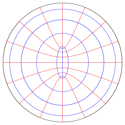
Figure 5: Coordinate curves $\xi=\mathrm{const.}$ and $\eta=\mathrm{const.}$

As $\xi$ and $\eta$ vary, these describe a family of hyperbolae and ellipses respectively. A plot of the coordinate curves in the $z-\rho$ plane is shown in Figure 5, where for convenience we allow $\rho$ to be negative.

Using equations (A-11) and (A-12), one can show that the metric on $\mathbb{H}^{3}$ in pseudospheroidal coordinates is

$$ds^{2}=\frac{\xi^{2}+\eta^{2}}{(\alpha^{2}-\xi^{2})(\beta^{2}-\xi^{2})}d\xi^{2}+\frac{\xi^{2}+\eta^{2}}{(\alpha^{2}+\eta^{2})(\beta^{2}+\eta^{2})}d\eta^{2}+\frac{\xi^{2}\eta^{2}}{\alpha^{2}\beta^{2}}d\phi^{2}$$ (A-18)

A.1.5 Pseudoparabolic Coordinates

For one-centre problems in flat space with a distinguished spatial direction, it is often useful to use parabolic coordinates. These may be thought of as spheroidal coordinates where one of the two centres has been allowed to recede to infinity, while the other is fixed at the origin. Again following Vozmischeva [45], we shall construct an analogous set of coordinates on $\mathbb{H}^{3}$ from the pseudospheroidal coordinates given above.

We first apply a Lorentz transformation to $\mathbb{E}^{3,1}$ in order to move the centre at $(\alpha,0,0,-\beta)$ to $(1,0,0,0)$. Without loss of generality we may write $\alpha=\cosh\frac{\psi}{2}$, $\beta=\sinh\frac{\psi}{2}$. The point at $(W,Z,P,\phi)$ moves to $(W^{\prime},Z^{\prime},P^{\prime},\phi^{\prime})$, where the new coordinates are related to the old by:

$$W = \cosh\frac{\psi}{2}W^{\prime}-\sinh\frac{\psi}{2}Z^{\prime},$$

$$Z = \cosh\frac{\psi}{2}Z^{\prime}-\sinh\frac{\psi}{2}W^{\prime},$$

$$P = P^{\prime},\qquad\quad\phi=\phi^{\prime}.$$ (A-19)

We also rescale the variables $\xi$ and $\eta$ by

$$\xi=\alpha\xi^{\prime}=\cosh\frac{\psi}{2}\xi^{\prime},\qquad\eta=\beta\eta^{\prime}=\sinh\frac{\psi}{2}\eta^{\prime}$$ (A-20)

In order to find the new coordinate surfaces, we substitute (A-19) and (A-20) into (A-14) and take the limit as $\psi\to\infty$, keeping terms of order $e^{-\psi}$. The new coordinate surfaces are then given by:

$$2Z^{\prime}(W^{\prime}-Z^{\prime}) = \frac{\xi^{\prime 2}}{1-\xi^{\prime 2}}(W^{\prime}-Z^{\prime})^{2}-\frac{1-\xi^{\prime 2}}{\xi^{\prime 2}}P^{\prime 2}=\mu^{2}(W^{\prime}-Z^{\prime})^{2}-\frac{P^{\prime 2}}{\mu^{2}}$$ (A-21)

$$2Z^{\prime}(W^{\prime}-Z^{\prime}) = -\frac{\eta^{\prime 2}}{1+\eta^{\prime 2}}(W^{\prime}-Z^{\prime})^{2}+\frac{1+\eta^{\prime 2}}{\eta^{\prime 2}}P^{\prime 2}=-\nu^{2}(W^{\prime}-Z^{\prime})^{2}+\frac{P^{\prime 2}}{\nu^{2}}$$ (A-22)

Where we have defined new coordinates $\mu=\frac{\xi^{\prime 2}}{1-\xi^{\prime 2}}$ and $\nu=\frac{\eta^{\prime 2}}{1+\eta^{\prime 2}}$. We now have no further use for the unprimed coordinates, so drop the primes. We can solve equations (A-21), (A-22), together with the pseudosphere constraint $W^{2}-P^{2}-Z^{2}=1$ to express the points on the pseudosphere in $\mathbb{E}^{3,1}$ in terms of $\mu$ and $\nu$. This gives

$$W=\frac{2+\mu^{2}-\nu^{2}}{2\sqrt{(1-\nu^{2})(1+\mu^{2})}},\quad P=\frac{\mu\nu}{\sqrt{(1-\nu^{2})(1+\mu^{2})}},\quad Z=\frac{\mu^{2}-\nu^{2}}{2\sqrt{(1-\nu^{2})(1+\mu^{2})}},$$ (A-23)

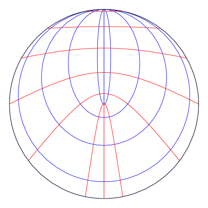
Figure 6: Coordinate curves $\mu=\mathrm{const.}$ and $\nu=\mathrm{const.}$

where

$$0\leq\mu<\infty,\qquad 0\leq\nu<1.$$ (A-24)

This time the coordinates cover the whole of $\mathbb{H}^{3}$. The sphere at infinity is given by $\nu=1$. We may once again use the gnomonic projection in order to visualise the coordinate surfaces as surfaces within the Beltrami ball model. We find that the Beltrami coordinates $z,\rho$ are given in terms of $\mu,\nu$ by:

$$z=\frac{Z}{W}=\frac{\mu^{2}-\nu^{2}}{2+\mu^{2}-\nu^{2}},\qquad\rho=\frac{P}{W}=\frac{\mu\nu}{2+\mu^{2}-\nu^{2}}.$$ (A-25)

Either from these equations, or from the projected versions of equations (A-21), (A-22), we find that the surfaces $\mu=\mathrm{const.}$ are hyperboloids and those of $\nu=\mathrm{const.}$ are ellipsoids. The plane $\phi=0$ is shown in Figure 6.

Using equations (A-23) and (A-11), it is a matter of straightforward calculation to find the metric on $\mathbb{H}^{3}$ in the $\mu,\nu,\phi$ coordinates. We find that

$$ds^{2}=\frac{\mu^{2}+\nu^{2}}{(1-\nu^{2})(1+\mu^{2})}\left[\frac{d\mu^{2}}{1+\mu^{2}}+\frac{d\nu^{2}}{1-\nu^{2}}+\frac{d\phi^{2}}{\mu^{-2}+\nu^{-2}}\right]$$ (A-26)

A.2 Horospheres

\begin{picture}(4816.0,4824.0)(2393.0,-6373.0)\end{picture}

Figure 7: A plot showing horospheres and their normal geodesics in Poincaré coordinates

When considering scattering processes in Euclidean space, the incoming wave is usually considered to be a plane wave, i.e. a wave whose phase is constant along any plane parallel to some vector. The important property of such planes is that they are everywhere normal to a set of parallel geodesics. Whether we are considering classical action waves or wavefunctions, the interpretation is that particles are moving parallel to some fixed direction. For hyperbolic space, we would like a similar set of waves to describe incoming particles initially parallel to some direction. In order to do this, we consider a pencil of parallel geodesics in $\mathbb{H}^{3}$, which meet at a point on $\partial\mathbb{H}^{3}$. The horospheres are a set of surfaces everywhere normal to these geodesics. It is most convenient to visualise these surfaces in the Poincaré ball model, since this is conformally flat so angles are as one would expect in Euclidean space. A set of parallel geodesics in this model are a set of circular arcs which meet the sphere $r=1$ orthogonally at some given point, say $(0,0,1)$. A surface which is everywhere normal to this pencil of geodesics is a sphere which is tangent to the sphere $r=1$ at the point $(0,0,1)$. A picture of the $y=0$ plane is shown in figure 7.

The horospheres may be thought of as a limit of a set of spheres in $\mathbb{H}^{3}$ whose centre goes to infinity whilst the radius also tends to infinity. The horospheres carry a natural Euclidean geometry and the restriction of the hyperbolic metric to each horosphere is flat, a result known as Wachter’s theorem [47, 48]. Clearly there is nothing special about our choice of boundary point, so there is a set of horospheres associated with every point on $S^{2}_{\infty}=\partial\mathbb{H}^{3}$.

A brief calculation shows that the horospheres associated with a pencil of parallel geodesics originating from $(0,0,1)$ are given in pseudoparabolic coordinates by the equation

$$(1+\mu^{2})(1-\nu^{2})=\mathrm{const.}$$ (A-27)

References

- [1] J. Bertrand, “Théorème relatif au mouvement d’un point attiré vers un centre fixe,” Compt. Rend. 77 (1873) 849.
- [2] H. Goldstein, “More on the prehistory of the Laplace or Runge-Lenz vector,” Am. J. Phys. 44 1123.
- [3] R. Lipschitz, Q. J. Pure Appl. Math. 12 (1873) 349.
- [4] W. Killing, “Die Mechanik in den Nicht-Euklidischen Raumformen,” J. Reine Angew. Math. 98 (1885) 1.
- [5] E. Schrodinger, “Eigenvalues and Eigenfunctions,” Proc. Roy. Irish Acad. (Sect. A) 46 (1940) 9.
- [6] P. W. Higgs, “Dynamical Symmetries In A Spherical Geometry. 1,” J. Phys. A 12 (1979) 309.
- [7] A. V. Shchepetilov “Comment on ”Central potentials on spaces of constant curvature: The Kepler problem on the two- dimensional sphere S2 and the hyperbolic plane H2” [J. Math. Phys. 46 (2005) 052702]” J. Math. Phys. 46 (2005) 114101
- [8] D. Zwanziger, “Exactly soluble nonrelativistic model of particles with both electric and magnetic charges,” Phys. Rev. 176 (1968) 1480.
- [9] H. V. Mcintosh and A. Cisneros, “Degeneracy in the presence of a magnetic monopole,” J. Math. Phys. 11 (1970) 896.
- [10] V. V. Gritsev, Yu. A. Kurochkin and V. S. Otchik, “Nonlinear symmetry algebra of the MIC-Kepler problem on the sphere ,” J. Phys. A: Math. and Gen. 33 (1979) 4903.
- [11] A. Nersessian and G. Pogosian, Phys. Rev. A 63 (2001) 020103 [arXiv:quant-ph/0006118].
- [12] Y. A. Kurochkin and V. S. Otchik “Symmetry and Interbasis Expansions in the MIC-Kepler problem in Lobachevsky Space” Nonlin. Phenom. in Compl. Syst. 8:1 (2005) 19
- [13] A. V. Borisov and I. S. Mamaev “Superintegrable systems on a sphere,” Regul. Chaotic. Dynam. 10 (3), (2005) 257
- [14] N. S. Manton, “A Remark On The Scattering Of Bps Monopoles,” Phys. Lett. B 110 (1982) 54.
- [15] M. F. Atiyah and N. J. Hitchin, “Low-energy scattering of nonAbelian magnetic monopoles,” Phil. Trans. Roy. Soc. Lond. A 315 (1985) 459.
- [16] G. W. Gibbons and N. S. Manton, “Classical And Quantum Dynamics Of BPS Monopoles,” Nucl. Phys. B 274 (1986) 183.
- [17] L. G. Feher and P. A. Horvathy, Phys. Lett. B 183 (1987) 182 [Erratum-ibid. 188B (1987) 512].
- [18] C. LeBrun, “Explicit Self-Dual Metrics on ,” J. Diff. Geom. 34 (1991) 223.
- [19] D. M. Austin and P. J. Braam, “Boundary values of hyperbolic monopoles,” Nonlinearity 3 (1990) 809.
- [20] M. F. Atiyah, “Magnetic monopoles in hyperbolic spaces” Proc. Bombay Colloq. 1984 on Vector Bundles on Algebraic Varieties (Oxford: Oxford University Press) 1-34.
- [21] N. S. Manton, “Monopole Interactions At Long Range,” Phys. Lett. B 154 (1985) 397 [Erratum-ibid. 157B (1985) 475].
- [22] M. F. Atiyah and N. J. Hitchin, “The Geometry And Dynamics Of Magnetic Monopoles. M.B. Porter Lectures,”
- [23] A. V. Shchepetilov, “Reduction of the two-body problem with central interaction on simply connected spaces of constant sectional curvature” J. Phys. A: Math. Gen. 31 (1998) 6297
- [24] A. J. Maciejewski and M. Przybylska “Non-integrability of restricted two body problems in constant curvature spaces,” Regul. Chaotic. Dynam. 8 (4), (2003) 413
- [25] O. Nash, “Differential geometry of monopole moduli spaces,” arXiv:math.dg/0610295.
- [26] G. W. Gibbons and N. S. Manton, “The moduli space metric for well separated BPS monopoles,” Phys. Lett. B 356 (1995) 32 [arXiv:hep-th/9506052].
- [27] H. Goldstein, C. Poole and J. Safko, Classical Mecanics, Addison Wesley, 2002.
- [28] S. A. Hartnoll and G. Policastro, arXiv:hep-th/0412044.
- [29] H. Pedersen and P. Tod, “Einstein metrics and hyperbolic monopoles,” Class. Quantum Grav. 8 (1991) 751.
- [30] I. M. Benn and P. Charlton, “Dirac symmetry operators from conformal Killing-Yano tensors,” Class. Quant. Grav. 14 (1997) 1037 [arXiv:gr-qc/9612011].
- [31] G. W. Gibbons and P. J. Ruback, “The Hidden Symmetries Of Taub-NUT And Monopole Scattering,” Phys. Lett. B 188 (1987) 226.
- [32] G. W. Gibbons and P. J. Ruback, “The Hidden Symmetries Of Multicenter Metrics,” Commun. Math. Phys. 115 (1988) 267.
- [33] J. de Boer, F. Harmsze and T. Tjin, “Nonlinear finite W symmetries and applications in elementary systems,” Phys. Rept. 272 (1996) 139 [arXiv:hep-th/9503161].
- [34] C. Quesne “On some nonlinear extensions of the angular momentum algebra,” J. Phys. A: Math. Gen. 28 (1995) 2847.
- [35] M. Roc̆ek “Representation theory of the nonlinear algebra,” Phys. Lett. B 255 (1991) 554
- [36] W. R. Hamilton “The hodograph, or a new method of expressing in symbolic language the Newtonian law of attraction,” Proc. Roy. Irish Acad. 3 (1847) 344.
- [37] J. L. Synge “Classical Dynamics” in Encyclopedia of Physics, ed. S. Flügge (Springer, Berlin, 1960), Vol. III/1.
- [38] E. G. P. Rowe “The Hamilton-Jacobi equation for Coulomb scattering,” Am. J. Phys. 53 (10), (1985) 997
- [39] E. G. P. Rowe “The classical limit of quantum mechanical Coulomb scattering,” J. Phys. A: Math. Gen. 20 (1987) 1419
- [40] G. W. Gibbons and P. J. Ruback, “Winding strings, Kaluza-Klein monopoles and Runge-Lenz vectors,” Phys. Lett. B 215 (1988) 653.
- [41] R. Gregory, J. A. Harvey and G. W. Moore, Adv. Theor. Math. Phys. 1 (1997) 283 [arXiv:hep-th/9708086].
- [42] D. N. Page, “Green’s Functions For Gravitational Multi - Instantons,” Phys. Lett. B 85 (1979) 369.
- [43] G. w. Meng, “The MICZ-Kepler problems in all dimensions,” arXiv:math-ph/0507029.
- [44] L. D. Landau and E. M. Lifshitz, Course of Theoretical Physics: Vol. 3 Quantum Mechanics – Non-relativistic theory, Pergamon 1959.
- [45] T. G. Vozmischeva, Integrable Problems of Celestial Mechanics in Spaces of Constant Curvature, Astrophysics and Space Science Library vol. 295, Kluwer Academic Publishers, 2003.
- [46] B. Carter, “Killing Tensor Quantum Numbers And Conserved Currents In Curved Space,” Phys. Rev. D 16 (1977) 3395.
- [47] W. Fenchel, Elementary Geometry in Hyperbolic Space, de Gruyter Studies in Mathematics 11, de Gruyter: Berlin, New York, 1989.
- [48] H. S. M. Coxeter, Non-Euclidean Geometry, University of Toronto Press, 1942