TIFR/TH/06-26

hep-th/0609017

Phases of unstable conifolds

K. Narayan

Department of Theoretical Physics,
Tata Institute of Fundamental Research,
Homi Bhabha Road, Colaba, Mumbai - 400005, India.
Email:  narayan@theory.tifr.res.in

We explore the phase structure induced by closed string tachyon condensation of toric nonsupersymmetric conifold-like singularities described by an integral charge matrix $Q=(n_{1}\ n_{2}-n_{3}-n_{4}),\ n_{i}>0,\ \sum_{i}Q_{i}\neq 0$, initiated in hep-th/0510104. Using gauged linear sigma model renormalization group flows and toric geometry techniques, we see a cascade-like phase structure containing decays to lower order conifold-like singularities, including in particular the supersymmetric conifold and the $Y^{pq}$ spaces. This structure is consistent with the Type II GSO projection obtained previously for these singularities. Transitions between the various phases of these geometries include flips and flops.

1 Introduction and summary

Understanding the stringy dynamics of nontrivial spacetime geometries is an interesting question, especially in the absence of spacetime supersymmetry. In this case, there typically are geometric instabilities in the system, often stemming from closed string tachyons in the theory (see e.g. [1, 2] for reviews), whose time dynamics is hard to unravel in detail. However understanding the detailed phase structure of these geometries is often tractable based on analyses of renormalization group flows in appropriate 2-dimensional gauged linear sigma models (GLSMs) [3] describing the system with unbroken $(2,2)$ worldsheet supersymmetry. In this case, such an analysis closely dovetails with the resolution of possible localized singularities present in the space.

A simple and prototypical example of such a renormalization group flow description of spacetime dynamics is the shrinking of a 2-sphere (${\mathbb{P}}^{1}$) given by $|\phi_{1}|^{2}+|\phi_{2}|^{2}=r//U(1)$. The complex coordinates $\phi_{i}$ have the $U(1)$ identifications $(\phi_{1},\phi_{2})\rightarrow(e^{i\theta}\phi_{1},e^{i\theta}\phi_{2})$, which we quotient by, to obtain a 2-sphere (this symplectic quotient construction will be elaborated on abundantly later). The parameter $r=R^{2}$ is the size of the sphere. The GLSM description of this system shows a 1-loop renormalization of the parameter $r$

$$r=r_{0}+2\log{\mu\over\Lambda}\ \qquad\equiv\qquad R^{2}=R_{0}^{2}-t\ .$$ (1)

In the equation on the right, we have recast the RG flow equation as an equation for the time evolution of the radius by identifying the RG scale $2\log{\mu\over\Lambda}\equiv-t$ ($\mu$ decreases along the RG flow) and $r_{0}$ with the initial size $R_{0}^{2}$. Early time ($t\sim 0$ here) corresponds to $\mu\sim\Lambda$ which in this case is $r\sim r_{0}\gg 0$, i.e. large $R\sim R_{0}$: more generally the sign of the coefficient of the logarithm dictates the direction of evolution of the geometry. The RG flow shows that the sphere has an instability to shrink, with the shrinking being slow initially since for large $R_{0}$, we have $R\sim R_{0}-{t\over 2R_{0}}+\ldots$.

This kind of behaviour also arises in the context of singular spaces in 3 complex dimensions where much more complicated and interesting phenomena happen. Two types of 3-dimensional nonsupersymmetric unstable singularities, particularly rich both in physical content and mathematical structure, are conifolds [4] and orbifolds [5, 6] (see also [7]), thought of as local singularities in some compact space, the full spacetime then being of the form ${\mathbb{R}}^{3,1}\times{\cal M}$. The conifold-like singularities [4] (reviewed in Sec. 2) are toric (as are orbifolds), labelled by a charge matrix

$$Q=(\begin{array}[]{cccc}n_{1}&n_{2}&-n_{3}&-n_{4}\end{array})\ ,\qquad\ \ \qquad\sum Q_{i}\neq 0\ ,$$ (2)

for integers $n_{i}>0$, which characterizes their toric data ($Q=(\begin{array}[]{cccc}1&1&-1&-1\end{array})$ corresponding to the supersymmetric conifold). The condition $\sum_{i}Q_{i}\neq 0$ implements spacetime supersymmetry breaking. It is possible to show that these are nonsupersymmetric orbifolds of the latter, and thus can be locally described by a hypersurface equation $z_{1}z_{4}-z_{2}z_{3}=0$, with the $z_{i}$ having discrete identifications from the quotienting. Generically these spaces are not complete intersections of hypersurfaces. They can be described as

$$\sum_{i}Q_{i}|\phi_{i}|^{2}=n_{1}|\phi_{1}|^{2}+n_{2}|\phi_{2}|^{2}-n_{3}|\phi_{3}|^{2}-n_{4}|\phi_{4}|^{2}=r\ //U(1)\ ,$$ (3)

where the $U(1)$ gauge group acts as $\phi_{i}\rightarrow e^{iQ_{i}\beta}\phi_{i}$ on the GLSM fields $\phi_{i}$, as will be described in detail later. The variations of the Fayet-Iliopoulos parameter $r$ describe the distinct phases of the geometry, with the $r\gg 0$ and $r\ll 0$ resolved phases giving fibrations over two topologically distinct 2-cycles. These $small$ $resolutions$ — Kähler blowups of the singularity (at $r=0$) by 2-cycles — have an asymmetry stemming from $\sum Q_{i}\neq 0$. Indeed the 1-loop renormalization $r=(\sum_{i}Q_{i})\log{\mu\over\Lambda}$ shows that one of these 2-spheres ${\mathbb{P}}^{1}_{-}$ is unstable to shrinking and the other, more stable, ${\mathbb{P}}^{1}_{+}$ grows. This spontaneous blowdown of a 2-cycle accompanied by the spontaneous blowup of a topologically distinct 2-cycle is a flip transition. Say at early times we set up the system in the unstable, approximately classical, (ultraviolet) phase where the shrinking 2-sphere ${\mathbb{P}}^{1}_{-}$ is large: then the geometry will dynamically evolve towards the more stable ${\mathbb{P}}^{1}_{+}$, with an inherent directionality in time, the singular region near $r=0$ where quantum (worldsheet instanton) corrections in the GLSM are large being a transient intermediate state.

An obvious question that arises on this analysis of [4] on the small resolutions is: are there RG evolution trajectories of a given unstable conifold-like singularity where the endpoints include the supersymmetric conifold, and more general lower order conifold-like singularities?
In this paper, we answer this question in the affirmative. Unlike the simple ${\mathbb{P}}^{1}$ example described in (1), there typically are orbifold singularities present on the ${\mathbb{P}}^{1}_{\pm}$ loci (as described in [4]), which are themselves unstable to resolving themselves, typically by blowups of 4-cycles (divisors) which can be interpreted as twisted sector tachyon states in the corresponding orbifold conformal field theories. For a large 2-sphere ${\mathbb{P}}^{1}_{-}$, the localized orbifold singularities on its locus are widely separated spatially. As this ${\mathbb{P}}^{1}_{-}$ shrinks, these pieces of spacetime potentially containing residual singularities come together, interact and recombine giving new spaces of distinct topology. The existence of both 2-cycle and various 4-cycle blowup modes of the conifold singularity besides those leading to the small resolutions makes the full phase structure given by the GLSM quite rich. This GLSM (also admitting $(2,2)$ worldsheet supersymmetry) with a $U(1)^{n+1}$ gauge group, for say $n$ additional 4-cycle blowup modes, is described by an enlarged charge matrix $Q_{i}^{a},\ a=1,\ldots,n+1$, with $n+1$ Fayet-Iliopoulos parameters $r_{a}$ controlling the vacuum structure, their RG flows describing the various phase transitions occurring in these geometries (a heuristic picture of the phase structure of a 2-parameter system is shown in Figure 1).

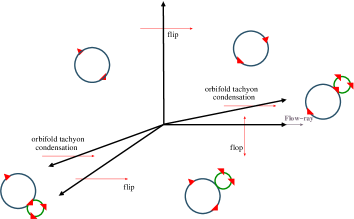
Figure 1: A heuristic picture of the phases of a 2-parameter system. The blue and green circles are ${\mathbb{P}}^{1}$s and weighted ${\mathbb{P}}^{2}$s respectively. The red triangles are residual orbifold singularities on their loci.

The geometry of the typical GLSM phase consists of combinations of 2-cycles and 4-cycles expanding/contracting in time, separating pieces of spacetime described by appropriate collections of coordinate charts glued together on their overlaps in accordance with the corresponding toric resolution (see Figures 3, 4). Besides flips and blowups of residual orbifold twisted sector tachyons, generic transitions between the various distinct phases include flops (marginal blowdowns/blowups of 2-cycles) – these arise along infrared moduli spaces. In such a case, the geometry can end up anywhere on this moduli space, including occasionally at (real) codimension-2 singularities on it: these correspond to lower order supersymmetric conifold-like spaces, e.g. the $Y^{pq}$ and $L^{a,b,c}$ spaces (see Sec.3).

As discussed in [4], the GLSM RG flow for a flip transition in fact always drives it in the direction of the (partial) resolution leading to a less singular residual geometry, i.e. a more stable endpoint. This enables a classification of the phases of the enlarged GLSMs discussed here corresponding to these unstable singularities into “stable” and “unstable” basins of attraction, noting the directionality of the RG trajectories involving potential flips, which always flow towards the more stable phases. The eventual stable phases typically consist of the stable 2-sphere ${\mathbb{P}}^{1}_{+}$ expanding in time, alongwith the various other expanding 4-cycles corresponding to the condensation of possible tachyons localized on the orbifold singularities on its locus: these phases include the various small resolutions of possible lower order conifold-like singularities. Since the GLSM with $(2,2)$ worldsheet supersymmetry has a smooth RG flow, the various phase transitions occurring in the evolution of the geometry are smooth.

A nontrivial GSO projection

$$\sum_{i}Q_{i}=even$$ (4)

was obtained in [4] for the ${\mathbb{R}}^{3,1}\times{\cal C}^{(flip)}$ spacetime background to admit a Type II string description with no bulk tachyons and admitting spacetime fermions. Here we show that the enlarged $Q_{i}^{a}$ charge matrix can be truncated appropriately so as to obtain a phase structure consistent with this Type II GSO projection. The final decay endpoints in Type II string theories are supersymmetric.

It is worth comparing these geometries to other simpler ones, e.g. ${\mathbb{C}}^{3}/{\mathbb{Z}}_{N}$ orbifold singularities [5, 6]. In the latter, the unstable blowup modes can be mapped explicitly to localized closed string tachyon states arising in the twisted sectors of the conformal field theories describing these orbifolds. A flip transition arises when a more dominant tachyon (more negative spacetime mass) condenses during the condensation of some tachyon, thus corresponding to a more relevant operator in the GLSM turning on during the RG flow induced by some relevant operator. Therefore a careful analysis of the closed string spectrum of the orbifold conformal field theory is in principle sufficient to understand the decay structure of the singularity. Generically such unstable orbifolds decay in a cascade-like fashion to lower order orbifold singularities which might themselves be unstable, and so on. In the present context of the conifold-like spaces, such a conformal field theory description is not easy to obtain in the vicinity of the singular region (which arises in the “middle” of the RG flows, unlike the orbifold cases). However since the conifold transition itself appears to be obstructed [4] (see footnote 4), it would seem that one could in principle use worldsheet techniques in the early time semiclassical regions to predict the full evolution structure. In this regard, the geometry/GLSM methods used here, aided by the structure of the residual orbifold singularities that arise in the small resolutions, are especially powerful in obtaining an explicit analysis. The GLSM description, dovetailing beautifully with the toric geometry description, gives detailed insights into the phase structure of these singularities (see Sec. 3). We analyze in detail some examples of singularities and exhibit a cascade-like phase structure containing lower order conifold-like singularities, including in particular the supersymmetric conifold and the $Y^{pq}$ spaces.

2 Some preliminaries on tachyons, flips and conifolds

In this section, we present some generalities on the nonsupersymmetric conifold-like singularities in question, largely reviewing results presented earlier in [4]. Consider a charge matrix

$$Q=\left(\begin{array}[]{cccc}n_{1}&n_{2}&-n_{3}&-n_{4}\end{array}\right)$$ (5)

and a ${\mathbb{C}}^{*}$ action on the complex coordinates $\Psi_{i}\equiv a,b,c,d$, with this charge matrix as $\Psi_{i}\rightarrow\lambda^{Q_{i}}\Psi_{i},\ \lambda\in{\mathbb{C}}^{*}$. Using the redefined coordinates $a^{1\over n_{1}},\ b^{1\over n_{2}},\ c^{1\over n_{3}},\ d^{1\over n_{4}}$, we find the invariant monomials

$$z_{1}=a^{1\over n_{1}}c^{1\over n_{3}},\ \ \ z_{2}=a^{1\over n_{1}}d^{1\over n_{4}},\ \ \ z_{3}=b^{1\over n_{2}}c^{1\over n_{3}},\ \ \ z_{4}=b^{1\over n_{2}}d^{1\over n_{4}}\ ,$$ (6)

satisfying locally

$$z_{1}z_{4}-z_{2}z_{3}=0\ ,$$ (7)

showing that the space is locally the supersymetric conifold. Globally however, the phases $e^{2\pi i/n_{k}}$ induced on the $z_{i}$ by the independent rotations on the underlying variables $a,b,c,d$, induce a quotient structure on the singularity with a discrete group $\Gamma$, the coordinates $z_{i}$ having the identifications

$$(\begin{array}[]{cccc}z_{1}&z_{2}&z_{3}&z_{4}\end{array})\ \longrightarrow^{a} (\begin{array}[]{cccc}e^{2\pi i/n_{1}}z_{1}&e^{2\pi i/n_{1}}z_{2}&z_{3}&z_{4}\end{array})\ ,$$ (10)

$$\longrightarrow^{b} (\begin{array}[]{cccc}z_{1}&z_{2}&e^{2\pi i/n_{2}}z_{3}&e^{2\pi i/n_{2}}z_{4}\end{array})\ ,$$ (12)

$$\longrightarrow^{c} (\begin{array}[]{cccc}e^{2\pi i/n_{3}}z_{1}&z_{2}&e^{2\pi i/n_{3}}z_{3}&z_{4}\end{array})\ ,$$ (14)

$$\longrightarrow^{d} (\begin{array}[]{cccc}z_{1}&e^{2\pi i/n_{4}}z_{2}&z_{3}&e^{2\pi i/n_{4}}z_{4}\end{array})\ .$$ (16)

Thus in general the flip conifold ${\cal C}^{(flip)}$ described by $Q=(\begin{array}[]{cccc}n_{1}&n_{2}&-n_{3}&-n_{4}\end{array})$ is the quotient

$${\cal C}^{(flip)}={{\cal C}\over\prod_{i}{\mathbb{Z}}_{n_{i}}}$$ (17)

of the supersymmetric conifold ${\cal C}$ with the action given by (10). As a toric variety described by this holomorphic quotient construction, this space can be described by relations between monomials of the variables $a,b,c,d$, invariant under the ${\mathbb{C}}^{*}$ action. In general, such spaces are not complete intersections of hypersurfaces, i.e. the number of variables minus the number of equations is not equal to the dimension of the space. The quotient structure above can be shown to obstruct the only complex structure deformation (locally given as $z_{1}z_{4}-z_{2}z_{3}=\epsilon$) of the supersymmetric conifold: there can of course be new abstract (non-toric) deformations which may not allow any interpretation in terms of the “upstairs” (quotient) structure.

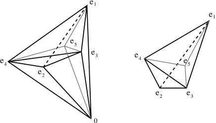
Figure 2: The toric fan for a nonsupersymmetric conifold-like singularity alongwith the two small resolutions $\{e_{1}e_{2}\},\{e_{3}e_{4}\}$, and an interior lattice point $e_{5}$.

A toric singularity corresponding to a charge matrix $Q$ can be described, as in Figure 2, by a strongly convex rational polyhedral cone defined by four lattice vectors $e_{i}$ satisfying the relation

$$\sum Q_{i}e_{i}=n_{1}e_{1}+n_{2}e_{2}-n_{3}e_{3}-n_{4}e_{4}=0$$ (18)

in a 3-dimensional $N$ lattice. Assuming any three, say $e_{1},e_{2},e_{3}$, of the four vectors $e_{i}$ define a non-degenerate volume, we see using elementary 3-dimensional vector analysis that

$$(e_{3}-e_{1})\cdot(e_{2}-e_{1})\times(e_{4}-e_{1})={(\sum_{i}Q_{i})\over n_{4}}\ e_{1}\cdot e_{2}\times e_{3}\ ,$$ (19)

so that the four lattice points $e_{i}$ are coplanar iff $\sum_{i}Q_{i}=0$. In this case these singularities are described as Calabi-Yau cones, corresponding to the $Y^{p,q}$ and $L^{a,b,c}$ spaces [12, 13].

By $SL(3,{\mathbb{Z}})$ transformations on the lattice, one can freely choose two of the $e_{i}$, and then find the other two consistent with the relation (18). Thus fixing, say, $e_{3},e_{4}$, we find

$$e_{1}=(-n_{2},n_{3}k,n_{4}k),\qquad e_{2}=(n_{1},n_{3}l,n_{4}l),\qquad e_{3}=(0,1,0),\qquad e_{4}=(0,0,1)\ ,$$ (20)

where $k,l$ are two integers satisfying $n_{1}k+n_{2}l=1$ (assuming $n_{1},n_{2}$ are coprime, $k,l$ always exist by the Euclidean algorithm).

For simplicity, we will restrict attention to the case $n_{1}=1$, which is sufficient for the physics we want to describe. In this case, we choose $k=1,l=0$, so that

$$e_{1}=(-n_{2},n_{3},n_{4}),\qquad e_{2}=(1,0,0),\qquad e_{3}=(0,1,0),\qquad e_{4}=(0,0,1)\ .$$ (21)

These singularities are isolated (point-like) if there are no lattice points on the “walls” of the toric cone. This is true if $n_{2}$ is coprime with both of $n_{3},n_{4}$, which can be seen as follows. If say $n_{2},n_{3}$ had common factors, i.e. say $n_{2}=m_{1}m_{2},n_{3}=m_{1}m_{3}$ for some factors $m_{i}$, then one can construct integral lattice points $re_{1}+se_{4},\ 0<r,s<1$, on the $\{e_{1}e_{4}\}$ wall: for example, taking $r={1\over m_{1}}$ and $s=1-\{{n_{4}\over m_{1}}\}$, we have $re_{1}+se_{4}=(-m_{2},m_{3},{n_{4}\over m_{1}}+s)=(-m_{2},m_{3},[{n_{4}\over m_{1}}]+1)\in\mbox{\boldmath$N$}$, lying on the $\{e_{1}e_{4}\}$ wall. Furthermore, since we can always write $n_{4}=m_{4}m_{1}+\nu$ for some $m_{4}$ and $\nu=0,1,\ldots,m_{1}-1$, we have $r+s={1\over m_{1}}+1-\{{n_{4}\over m_{1}}\}<1$ if $n_{4}\neq m_{4}m_{1}$ ($\nu\neq 0$), i.e. the point $re_{1}+se_{4}$ lies strictly in the interior of the $\{e_{1}e_{4}\}$ wall (if $n_{4}=m_{4}m_{1}$, the interior point $(-m_{2},m_{3},m_{4})={1\over m_{1}}e_{1}$ exists). Similarly, if $n_{2},n_{4}$ have common factors, then there are lattice points in the interior of the $\{e_{1}e_{3}\}$ wall. Note that if $n_{3},n_{4}$ have common factors, there potentially are lattice points on the internal $\{e_{1},e_{2}\}$ wall.

There is a nice description of the physics of such a geometry as the Higgs branch of the moduli space of a $U(1)$ gauged linear sigma model admitting $(2,2)$ worldsheet supersymmetry with four scalar superfields $\Psi\equiv\phi_{1},\phi_{2},\phi_{3},\phi_{4}$, and a Fayet-Iliopoulos (real) parameter $r$. The fields $\Psi$ transform under $U(1)$ gauge transformations with the charge matrix $Q_{i}$ as

$$\Psi_{i}\rightarrow e^{iQ_{i}\beta}\Psi_{i},\qquad\qquad Q_{i}=(n_{1},n_{2},-n_{3},-n_{4})\ ,$$ (22)

$\beta$ being the gauge parameter. The action for the GLSM is (using conventions of [3, 10])

$$S=\int d^{2}z\ \biggl{[}d^{4}\theta\ \biggl{(}{\bar{\Psi}_{i}}e^{2Q_{i}V}\Psi_{i}-{1\over 4e^{2}}{\bar{\Sigma}}\Sigma\biggr{)}+\mathop{\rm Re}\biggl{(}it\int d^{2}{\tilde{\theta}}\ \Sigma\biggr{)}\biggr{]}\ ,$$ (23)

where $t=ir+{\theta\over 2\pi}$ , $\theta$ being the $\theta$-angle in $1+1$-dimensions, and $e$ being the gauge coupling. The twisted chiral superfields $\Sigma_{a}$ (whose bosonic components include complex scalars $\sigma_{a}$) represent field-strengths for the gauge fields. The classical vacuum structure can be found from the bosonic potential

$$U=\sum_{a}{(D)^{2}\over 2e^{2}}+2{\bar{\sigma}}\sigma\sum_{i}Q_{i}Q_{i}|\Psi_{i}|^{2}\ .$$ (24)

Then $U=0$ requires $D=0$: solving this for $r\neq 0$ gives expectation values for the $\Psi_{i}$, which Higgs the gauge group down to some discrete subgroup and lead to mass terms for the $\sigma$ whose expectation value thus vanishes. The classical vacuum structure is then described by the D-term equation

$$-{D\over e^{2}}=\sum_{i}Q_{i}|\Psi_{i}|^{2}=n_{1}|\phi_{1}|^{2}+n_{2}|\phi_{2}|^{2}-n_{3}|\phi_{3}|^{2}-n_{4}|\phi_{4}|^{2}=r\ //U(1)\ ,$$ (25)

from which one can realize the two small resolutions (Kähler blowups by 2-cycles) as rank-2 bundles over ${\mathbb{P}}^{1}_{\pm}$, as manifested by the GLSM moduli space for the single FI parameter ranges $r\gg 0$ and $r\ll 0$. These small resolutions are described in the toric fan by the $\{e_{1},e_{2}\}$ and $\{e_{3},e_{4}\}$ subdivisions: e.g. the $\{e_{3},e_{4}\}$ subdivision giving residual subcones $C(0;e_{2},e_{3},e_{4}),\ C(0;e_{1},e_{3},e_{4})$, is described by the coordinate charts $\{(\phi_{2},\phi_{3},\phi_{4}),\ (\phi_{1},\phi_{3},\phi_{4})\}$. The FI parameter $r$ has a 1-loop renormalization given by

$$r=\biggl{(}{\sum_{i}Q_{i}\over 2\pi}\biggr{)}\log{\mu\over\Lambda}=\left({\Delta V\over 2\pi}\right)\log{\mu\over\Lambda}\ ,$$ (26)

showing that for $\sum_{i}Q_{i}\neq 0$, the GLSM RG flow drives the system away from the shrinking 2-sphere ${\mathbb{P}}^{1}_{-}$, towards the phase corresponding to the growing 2-sphere ${\mathbb{P}}^{1}_{+}$. This dynamical evolution process executing a flip transition mediates mild dynamical topology change since the blown-down 2-cycle ${\mathbb{P}}^{1}_{-}$ and blown-up 2-cycle ${\mathbb{P}}^{1}_{+}$ have distinct intersection numbers with various cycles in the geometry.
The geometric structure of the residual coordinate charts can be gleaned from the toric fan. From the Smith normal form algorithm of [5] (or otherwise), we can see that the various residual subcones correspond to the orbifolds $C(0;e_{1},e_{2},e_{3})\equiv{\mathbb{Z}}_{n_{4}}(1,n_{2},-n_{3})$, $C(0;e_{1},e_{2},e_{4})\equiv{\mathbb{Z}}_{n_{3}}(1,n_{2},-n_{4})$, and $C(0;e_{1},e_{3},e_{4})\equiv{\mathbb{Z}}_{n_{2}}(1,-n_{3},-n_{4})$, up to shifts of the orbifold weights by the respective orbifold orders, since these cannot be determined unambiguously by the Smith algorithm. Using this, one can see that a consistent Type II GSO projection

$$\Delta n=\sum Q_{i}=n_{1}+n_{2}-n_{3}-n_{4}=even$$ (27)

can be assigned to the conifold-like singularity in question, from the known Type II GSO projection $\sum k_{i}=even$ [5] on the ${\mathbb{C}}^{3}/{\mathbb{Z}}_{M}(k_{1},k_{2},k_{3})$ residual orbifolds, if we make the reasonable assumption that a GSO projection defined for the geometry is not broken along the RG flows describing the decay channels.

In what follows, we will examine the phase structure of these singularities in greater detail using their description in terms of toric geometry and GLSMs. In particular we exhibit a cascade-like phase structure for a singularity with given charge matrix $Q$, containing lower order singularities $Q^{\prime}$ with smaller $\sum_{i}Q_{i}^{\prime}$, consistent with the above GSO projection.

3 The phases of unstable conifolds

In this section, we will study the full phase structure of the unstable conifold-like singularities in question using GLSMs and toric geometry techniques. The prime physical observation is that the intermediate endpoint geometries arising in the small resolution decay channels above can contain additional blowup modes (interpreted as twisted sector tachyons if these are residual orbifold singularities), which further continue the evolution of the full geometry. Since these additional blowup modes are present in the original conifold-like singularity, there can in principle exist new decay channels corresponding to first blowing up these modes. Technically this is because the toric fan for such a singularity potentially contains in its interior one or more lattice points, since the residual subcones are potentially singular if their $N$ lattice volumes are greater than unity. Thus in addition to the small resolution subdivisions [4] reviewed above, the cone $C(0;e_{1},e_{2},e_{3},e_{4})$ defining the conifold-like singularity can also be subdivided using these interior lattice points. In the case of orbifold singularities, the spacetime masses of tachyons, corresponding to worldsheet R-charges of the appropriate twisted sector operators in the orbifold conformal field theory, effectively grade the decay channels. Since there is no such tractable conformal field theory description for the conifold-like geometries themselves (in the vicinity of the singularity), it is difficult to a priori identify their most dominant evolution channels. However one can efficiently resort to GLSM renormalization group techniques (developed for unstable 3-dimensional orbifolds in [6]) which essentially describe the full phase structure of these geometries and the possible evolution patterns to the final stable endpoints. We will first discuss the toric geometry description and then describe some generalities of the corresponding GLSM.

Consider a singularity with charge matrix $Q$ described by the cone defined by the $e_{i},\ i=1,\ldots,4$, with one relation $\sum_{i}Q_{i}e_{i}=0$ in the 3-dimensional $N$ lattice. For simplicity, we restrict attention to singularities with $n_{1}=1$, i.e. of the form $Q=(\begin{array}[]{cccc}1&n_{2}&-n_{3}&-n_{4}\end{array})$, with the $e_{i}$ given by (21). Then as described in the previous section, there always exist two topologically distinct (asymmetric) small resolutions corresponding to the subdivisions $\{e_{1}e_{2}\}$ and $\{e_{3}e_{4}\}$: the subdivision $\{e_{3}e_{4}\}$ gives a less singular residual geometry (smaller $N$ lattice subcone volumes) if $n_{1}+n_{2}<n_{3}+n_{4}$. We can obtain detailed insight into the structure of the fan by taking recourse to the structure of the ${\mathbb{C}}^{3}/{\mathbb{Z}}_{N}$ orbifold singularities arising in these small resolution subdivisions using the techniques and results of [5], reviewed in Appendix A. The basic point is that there exists a precise correspondence between operators in the orbifold conformal field theory and $N$ lattice points in the interior of (i.e. on or below the affine hyperplane $\Delta$, described in Appendix A; see Figure 5) the toric cone representing the orbifold. Thus $N$ lattice points in a given subcone of the toric cone, corresponding to specific blowup modes of the singularity, precisely map to tachyons or moduli arising in twisted sectors of the orbifold conformal field theory corresponding to the subcone.

Now by an interior lattice point of the conifold-like cone $C(0;e_{1},e_{2},e_{3},e_{4})$ (see Figure 2), we mean lattice points in the interior of the subcone $C(0;e_{1},e_{3},e_{4})$ arising in the stable small resolution (for $n_{1}+n_{2}<n_{3}+n_{4}$). Any other point in the interior of say subcones $C(0;e_{1},e_{2},e_{3})$ or $C(0;e_{1},e_{2},e_{4})$ but not $C(0;e_{1},e_{3},e_{4})$ is effectively equivalent to an irrelevant operator from the GLSM point of view. Now if there exists a lattice point $e_{5}$ in the interior of the cone $C(0;e_{1},e_{2},e_{3},e_{4})$, then there are two independent relations between these five vectors $e_{i},\ i=1,\ldots,5$ in the 3-dimensional lattice $N$: these can be chosen as a basis for all possible relations between these vectors. These relations

$$\sum_{i}Q_{i}^{a}e_{i}=0$$ (28)

define a charge matrix $Q_{i}^{a}$: changing the basis of relations amounts to changing a row of $Q_{i}^{a}$ to a rational linear combination of the two rows also having integral charges. Similarly, $n$ extra lattice points in the interior of the cone give $n+1$ relations between the $e_{i},\ i=1,\ldots,4+n$, thus defining a $(n+1)\times(4+n)$ charge matrix $Q_{i}^{a}$. Specifying the structure of this $Q_{i}^{a}$ is equivalent to giving all the information contained in the toric fan of the singularity. For example, if there exists a single extra lattice point $e_{5}$ in the interior of the subcone $C(0;e_{1},e_{3},e_{4})\equiv{\mathbb{Z}}_{n_{2}}$, then there is a relation of the form $e_{5}={1\over n_{2}}(m_{1}e_{1}+m_{3}e_{3}+m_{4}e_{4}),\ m_{i}>0$, defining a row $Q_{i}^{2}=(\begin{array}[]{ccccc}m_{1}&0&m_{3}&m_{4}&-n_{2}\end{array})$. This point corresponds to a tachyon if $\sum_{i}m_{i}<n_{2}$. Thus the combinatorics of $Q_{i}^{a}$ determines the geometry of the toric fan, e.g. whether $e_{5}$ is contained in the intersection of subcones say $C(0;e_{1},e_{3},e_{4})$ and $C(0;e_{1},e_{2},e_{3})$, and so on.

Furthermore in Type II theories, there is a nontrivial GSO projection that acts nontrivially on these lattice points, preserving only some of them physically: this may be thought of as arising from the GSO projections in the orbifold theories corresponding to the subcones arising under the small resolutions. Thus an interior lattice point may not in fact correspond to any blowup mode that actually exists in the physical theory. A simple way to encode the consequences of this GSO projection is to ensure that each row of the charge matrix $Q_{i}^{a}$ in the GLSM for the physical Type II theory sums to an even integer

$$\sum_{i}Q_{i}^{a}=even\ ,\qquad\ a=1,\ldots,n+1\ .$$ (29)

It is easy to see that this Type II truncation of $Q_{i}^{a}$ retaining only rows with even sum is consistent (and we will elaborately describe this in examples later): e.g. in the example above, the point $e_{5}\in C(0;e_{1},e_{3},e_{4})$ given by $e_{5}={1\over n_{2}}(m_{1}e_{1}+m_{3}e_{3}+m_{4}e_{4})$ defines a new conifold-like subcone $C(0;e_{5},e_{2},e_{3},e_{4})$, corresponding to a charge matrix $Q^{\prime}$, which admits a Type II GSO projection iff $\sum_{i}Q_{i}^{\prime}=even$. This constraint effectively arises from the GSO projection on the point $e_{5}$ thought of as a twisted sector state in the orbifold corresponding to the subcone $C(0;e_{1},e_{3},e_{4})$.

The full phase structure of such a geometry is obtained by studying an enlarged GLSM with gauge group $U(1)^{n+1}$ with $4+n$ superfields $\Psi_{i}$ and $n+1$ Fayet-Iliopoulos parameters $r_{a}$. Much of the remainder of this section is a direct generalization of the techniques described in [6] to the conifold-like singularities in question here: we present a detailed discussion primarily for completeness. The action of such a GLSM (in conventions of [3, 10]) is

$$S=\int d^{2}z\ \biggl{[}d^{4}\theta\ \biggl{(}{\bar{\Psi}_{i}}e^{2Q_{i}^{a}V_{a}}\Psi_{i}-{1\over 4e_{a}^{2}}{\bar{\Sigma}_{a}}\Sigma_{a}\biggr{)}+\mathop{\rm Re}\biggl{(}it_{a}\int d^{2}{\tilde{\theta}}\ \Sigma_{a}\biggr{)}\biggr{]}\ ,$$ (30)

where summation on the index $a=1,\ldots,n+1$ is implied. The $t_{a}=ir_{a}+{\theta_{a}\over 2\pi}$  are Fayet-Iliopoulos parameters and $\theta$-angles for each of the $n+1$ gauge fields ($e_{a}$ being the gauge couplings). The twisted chiral superfields $\Sigma_{a}$ (whose bosonic components are complex scalars $\sigma_{a}$) represent field-strengths for the gauge fields. The action of the $U(1)^{n+1}$ gauge group on the $\Psi_{i}$ is given in terms of the $(n+1)\times(4+n)$ charge matrix $Q_{i}^{a}$ above as

$$\Psi_{i}\rightarrow e^{iQ_{i}^{a}\lambda}\ \Psi_{i}\ ,\qquad Q_{i}^{a}=\left(\begin{array}[]{ccccccc}n_{1}&n_{2}&-n_{3}&-n_{4}&0&\ldots\\ 0&q_{2}^{2}&-q_{3}^{2}&-q_{4}^{2}&q_{5}^{2}&\ldots\\ &&\cdot&&&\ldots\\ &&\cdot&&&\ldots\\ \end{array}\right),\qquad\ a=1,\ldots,n+1\ .$$ (31)

Such a charge matrix only specifies the $U(1)^{n+1}$ action up to a finite group, due to the possibility of a ${\mathbb{Q}}$-linear combination of the rows of the matrix also having integral charges. The specific form of $Q_{i}^{a}$ is chosen to conveniently illustrate specific geometric substructures: for example, the second row above, with $q_{1}^{2}=0$, describes the conifold-like subcone $C(0;e_{2},e_{3},e_{4},e_{5})$. The variations of the $n+1$ independent FI parameters control the vacuum structure of the theory. The space of classical ground states of this theory can be found from the bosonic potential

$$U=\sum_{a}{(D_{a})^{2}\over 2e_{a}^{2}}+2\sum_{a,b}{\bar{\sigma}}_{a}\sigma_{b}\sum_{i}Q_{i}^{a}Q_{i}^{b}|\Psi_{i}|^{2}\ .$$ (32)

Then $U=0$ requires $D_{a}=0$: solving these for $r_{a}\neq 0$ gives expectation values for the $\Psi_{i}$, which Higgs the gauge group down to some discrete subgroup and lead to mass terms for the $\sigma_{a}$ whose expectation values thus vanish. The classical vacua of the theory are then given in terms of solutions to the D-term equations

$${-D_{a}\over e^{2}}=\sum_{i}Q_{i}^{a}|\Psi_{i}|^{2}-r_{a}=0\ ,\qquad a=1,\ldots,n+1\ .$$ (33)

At the generic point in $r$-space, the $U(1)^{n+1}$ gauge group is completely Higgsed, giving collections of coordinate charts that characterize in general distinct toric varieties. In other words, this $(n+1)$-parameter system admits several “phases” (convex hulls in $r$-space, defining the secondary fan) depending on the values of the $r_{a}$. At boundaries between these phases where some (but not all) of the $r_{a}$ vanish, some of the $U(1)$s survive giving rise to singularities classically. Each phase is an endpoint since if left unperturbed, the geometry can remain in the corresponding resolution indefinitely (within this noncompact approximation): in this sense, each phase is a fixed point of the GLSM RG flow. However some of these phases are unstable while others are stable, in the sense that fluctuations (e.g. blowups/flips of cycles stemming from instabilities) will cause the system to run away from the unstable phases towards the stable ones. This can be gleaned from the 1-loop renormalization of the FI parameters

$$r_{a}=\bigg{(}{\sum_{i}Q_{i}^{a}\over 2\pi}\bigg{)}\log{\mu\over\Lambda}\ ,$$ (34)

where $\mu$ is the RG scale and $\Lambda$ is a cutoff scale where the $r_{a}$ are defined to vanish. A generic linear combination of the gauge fields coupling to a linear combination $\sum_{a}\alpha_{a}r_{a}$ of the FI parameters, the $\alpha_{a}$ being arbitrary real numbers, has a 1-loop running whose coefficient vanishes if

$$\sum_{\alpha=1}^{n+1}\sum_{i=1}^{n+4}\alpha_{a}Q_{i}^{a}=0\ ,$$ (35)

in which case the linear combination is marginal. This equation defines a codimension-one hyperplane perpendicular to a ray, called the Flow-ray, emanating from the origin and passing through the point $(-\sum_{i}Q_{i}^{1},-\sum_{i}Q_{i}^{2},\ldots,-\sum_{i}Q_{i}^{n+1})$ in $r$-space which has real dimension $n+1$. Using the redefinition ${Q_{i}^{a}}^{\prime}\equiv(\sum_{i}Q_{i}^{1})Q_{i}^{a}-(\sum_{i}Q_{i}^{a})Q_{i}^{1},\ a\neq 1$, we see that $\sum_{i}{Q_{i}^{a}}^{\prime}=(\sum_{i}Q_{i}^{1})(\sum_{i}Q_{i}^{a})-(\sum_{i}Q_{i}^{a})(\sum_{i}Q_{i}^{1})=0$,  for $a\neq 1$,  so that the FI parameters coupling to these redefined $n$ gauge fields have vanishing 1-loop running. Thus there is a single relevant direction (along the flow-ray) and an $n$-dimensional hyperplane of the $n$ marginal directions in $r$-space. By studying various linear combinations $\sum_{a}\alpha_{a}r_{a}$, we see that the 1-loop RG flows drive the system along the single relevant direction to the phases in the large $r$ regions of $r$-space, i.e., $r_{a}\gg 0$ (if none of the $r_{a}$ is marginal), that are adjacent to the Flow-ray  $F\equiv(-\sum_{i}Q_{i}^{1},-\sum_{i}Q_{i}^{2},\ldots,-\sum_{i}Q_{i}^{n+1})$, or contain it in their interior: these are the stable phases.

Reversing this logic, we see that the direction precisely opposite to the Flow-ray, i.e. $-F\equiv(\sum_{i}Q_{i}^{1},\sum_{i}Q_{i}^{2},\ldots,\sum_{i}Q_{i}^{n+1})$, defines the ultraviolet of the theory. This ray will again lie either in the interior of some one convex hull or adjoin multiple convex hulls. This ray $-F$ corresponds to the maximally unstable direction which is generically the unstable small resolution ${\mathbb{P}}^{1}_{-}$, defining the ultraviolet of the theory (see the examples that follow). This is because any of the residual localized orbifold singularities on this ${\mathbb{P}}^{1}_{-}$ locus can be further resolved (if unstable) by turning on the corresponding FI parameter, which process is along the Flow-ray direction.

We restrict attention to the large $r_{a}$ regions, thus ignoring worldsheet instanton corrections: this is sufficient for understanding the phase structure, and consistent for initial values of $r_{a}$ whose components in the marginal directions lie far from the center of the marginal $n$-plane.

The 1-loop renormalization of the FI parameters can be expressed [3, 14, 10] in terms of a perturbatively quantum-corrected twisted chiral superpotential for the $\Sigma_{a}$ for a general $n+1$-parameter system, obtained by considering the large-$\sigma$ region in field space and integrating out those scalars $\Psi_{i}$ that are massive here (and their expectation values vanish energetically). This leads to the modified potential

$$U(\sigma)={e^{2}\over 2}\sum_{a=1}^{n+1}\bigg{|}i{\hat{\tau}}_{a}-{\sum_{i=1}^{4+n}Q_{i}^{a}\over 2\pi}(\log(\sqrt{2}\sum_{b=1}^{n+1}Q_{i}^{b}\sigma_{b}/\Lambda)+1)\bigg{|}^{2}\ .$$ (36)

The singularities predicted classically at the locations of the phase boundaries arise from the existence of low-energy states at large $\sigma$. The physics for the nonsupersymmetric cases here is somewhat different from the cases where $\sum_{i}Q_{i}^{a}=0$ for all $a$, as discussed in general in [3, 14, 10] (and for orbifold flips in [6]). Consider the vicinity of such a singularity at a phase boundary but far from the (fully) singular region where all $r_{a}$ are zero, and focus on the single $U(1)$ (with say charges $Q_{i}^{1}$) that is unbroken there (i.e. we integrate out the other $\sigma_{a},\ a\neq 1$, by setting them to zero). Now if $\sum_{i}Q_{i}^{1}=0$ (i.e. unbroken spacetime supersymmetry), then there is a genuine singularity when $U(\sigma)={e^{2}\over 2}|i{\hat{\tau}}_{a}-{1\over 2\pi}\sum_{i}Q_{i}^{1}\log|Q_{i}^{1}||^{2}=0$, and if $\sum_{i}Q_{i}^{a}=0$ for all $a$, this argument can be applied to all of the $U(1)$s. However for the nonsupersymmetric cases here, we have $\sum_{i}Q_{i}^{a}\neq 0$: so if say $\sum_{i}Q_{i}^{1}\neq 0$ (with the other $Q_{i}^{a}$ redefined to ${Q_{i}^{a}}^{\prime}$ with $\sum_{i}{Q_{i}^{a}}^{\prime}=0$), then along the single relevant direction where $\sum_{i}Q_{i}^{1}\neq 0$, the potential energy has a $|\log\sigma_{1}|^{2}$ growth. Thus the field space accessible to very low-lying states is effectively compact (for finite worldsheet volume) and there is no singularity for any $r_{a},\theta_{a}$, along the RG flow: in other words, the RG flow is smooth along the relevant direction for all values of $\tau_{1}$, and the phase boundaries do not indicate singularities.

Thus the overall physical picture is the following: the generic system in question begins life at early times in the ultraviolet phase, typically the unstable 2-sphere ${\mathbb{P}}^{1}_{-}$ which has a tendency to shrink. If this 2-sphere size is large, then this is an approximately classical phase of the theory, with the shrinking being very slow initially. This ${\mathbb{P}}^{1}_{-}$ typically has residual localized orbifold singularities which are widely separated for a large ${\mathbb{P}}^{1}_{-}$. As the 2-sphere shrinks, tachyons localized at these orbifolds might condense resolving the latter by 4-cycle blowup modes. As the system evolves, these various cycles interact and recombine potentially via several topology-changing flip transitions until the geometry ultimately settles down into any of the stable phases (which typically have distinct topology). A stable phase typically consists of the stable 2-sphere ${\mathbb{P}}^{1}_{+}$ growing in time, with the various possible orbifold singularities on its locus resolving themselves by tachyon condensation. The transitions occurring in the course of this evolution between various phases are smooth as discussed above.

In what follows, we describe two 2-parameter examples in some detail illustrating the above generalities: one corresponds to a singularity that has a unique late-time endpoint (within this 2-parameter approximation), while the other includes the supersymmetric conifold in its final endpoints, thus exhibiting infrared moduli representing the flop between the two topologically distinct small resolutions of the latter. Before doing so, we mention a simple example of a singularity which has no interior lattice point (as defined earlier), and evolves to its stable small resolution. The singularity $Q=(\begin{array}[]{cccc}1&1&-1&-3\end{array})$ is the simplest unstable Type II conifold-like singularity. The stable small resolution given by the subdivision $\{e_{3}e_{4}\}$ completely resolves the singularity, since the subcone $C(0,e_{1},e_{3},e_{4})$, potentially an orbifold singularity, is in fact smooth. The other small resolution gives rise to the orbifold subcone $C(0,e_{1},e_{2},e_{3})\equiv{\mathbb{Z}}_{3}(1,1,2)$ which is effectively supersymmetric since its only GSO-preserved blowup mode is a marginal twisted sector state arising in one of the anti-chiral rings (the subcone $C(0,e_{1},e_{2},e_{4})$ is smooth).

3.1 Decays to a single stable phase

Consider the singularity $Q=(\begin{array}[]{cccc}1&7&-5&-19\end{array})$ (see Figure 3). The subcones can be identified as the following Type II orbifolds:

$$C(0;e_{1},e_{2},e_{3})\equiv{\mathbb{Z}}_{19}(1,7,14)\ ,\ C(0;e_{1},e_{2},e_{4})\equiv{\mathbb{Z}}_{5}(1,2,1)\ ,\ C(0;e_{1},e_{3},e_{4})\equiv{\mathbb{Z}}_{7}(1,2,-5)\ ,$$ (37)

while $C(0;e_{2},e_{3},e_{4})$ is of course smooth. It is straightforward to see that

$$e_{5}\equiv(-1,1,3)={1\over 7}(e_{1}+2e_{3}+2e_{4})\ \ \in\ \ C(0;e_{1},e_{3},e_{4})$$ (38)

corresponds to the tachyon in the twisted sector $j=1$, having R-charge $R_{j}=({1\over 7},{2\over 7},{2\over 7})$ (GSO preserved since $E_{j}=-1$ using (61)). Including this lattice point gives the charge matrix

$$Q_{i}^{a}=\left(\begin{array}[]{ccccc}1&7&-5&-19&0\\ 0&1&-1&-3&1\\ \end{array}\right)\ ,$$ (39)

where we have used the conifold-like relation $e_{2}+e_{5}-e_{3}-3e_{4}=0$ to define the second row. Note $\sum_{i}Q_{i}^{a}=even,\ a=1,2$, incorporating the GSO projection. One could equally well have defined the second row in $Q_{i}^{a}$ as $(\begin{array}[]{ccccc}1&0&2&2&-7\end{array})$ noticing as above that $e_{5}\in C(0;e_{1},e_{3},e_{4})$: this does not change the physics.

To understand the phase structure of this theory, let us analyze the D-term equations (suppressing the gauge couplings)

$$-D_{1} = |\phi_{1}|^{2}+7|\phi_{2}|^{2}-5|\phi_{3}|^{2}-19|\phi_{4}|^{2}-r_{1}=0\ ,$$

$$-D_{2} = |\phi_{2}|^{2}+|\phi_{5}|^{2}-|\phi_{3}|^{2}-3|\phi_{4}|^{2}-r_{2}=0\ .$$ (40)

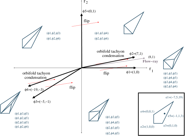
Figure 3: Phases of $Q=(1\ 7\ -5\ -19)$, with the toric subdivisions and corresponding coordinate charts in each phase, as well as the RG flow directions and the physics of each phase boundary.

There are three other auxiliary D-terms too:

$$-D_{2}^{\prime} = -D_{1}+7D_{2}=|\phi_{1}|^{2}+2|\phi_{3}|^{2}+2|\phi_{4}|^{2}-7|\phi_{5}|^{2}-(r_{1}-7r_{2})=0\ ,$$

$$-D_{3}^{\prime} = -D_{1}+5D_{2}=|\phi_{1}|^{2}+2|\phi_{2}|^{2}-4|\phi_{4}|^{2}-5|\phi_{5}|^{2}-(r_{1}-5r_{2})=0\ ,$$ (41)

$$-D_{4}^{\prime} = -3D_{1}+19D_{2}=3|\phi_{1}|^{2}+2|\phi_{2}|^{2}+4|\phi_{3}|^{2}-19|\phi_{5}|^{2}-(3r_{1}-19r_{2})=0\ .$$

These are obtained by looking at different linear combinations of the two $U(1)$s that do not couple to some subset of the chiral superfields: e.g. the $U(1)$s giving $D_{2}^{\prime}$ and $D_{3}^{\prime}$ do not couple to $\phi_{2}$ and $\phi_{3}$ respectively. These D-terms show that the five rays drawn from the origin $(0,0)$ out through the points $\phi_{1}\equiv(1,0),\ \phi_{2}\equiv(7,1),\ \phi_{3}\equiv(-5,-1),\ \phi_{4}\equiv(-19,-3),\ \phi_{5}\equiv(0,1)$, are phase boundaries: e.g. at the boundary $(7,1)$, the $U(1)$ coupling to $r_{1}-7r_{2}$ is unHiggsed, signalling a classical singularity due to the existence of a new $\sigma$-field direction.

Before analyzing the phase structure, let us can gain some insight into the geometry of this singularity. In the holomorphic quotient construction, introduce coordinates $x_{i},\ i=1,\ldots,5$, corresponding to the lattice points $e_{i}$ subject to the quotient action $x_{i}\rightarrow\lambda^{Q_{i}^{a}}x_{i}$ with $Q_{i}^{a}$ given in (39). Then the divisors $x_{i}=0,\ i=1,2,3,4$, are noncompact divisors, while the divisor $x_{5}=0$ is a compact one, whose structure can be gleaned as follows: the $({\mathbb{C}}^{*})^{2}$ action is

$$g_{1}:\ (x_{1},x_{2},x_{3},x_{4},x_{5})\ \sim (\lambda x_{1},\lambda^{7}x_{2},\lambda^{-5}x_{3},\lambda^{-19}x_{4},x_{5})\ ,$$

$$g_{2}:\ (x_{1},x_{2},x_{3},x_{4},x_{5})\ \sim (x_{1},\lambda x_{2},\lambda^{-1}x_{3},\lambda^{-3}x_{4},\lambda x_{5})\ ,$$ (42)

so that on $x_{5}=0$, the group element $g_{1}g_{2}^{-7}(\lambda)$ has action

$$(x_{1},x_{2},x_{3},x_{4},0)\ \sim\ (\lambda x_{1},x_{2},\lambda^{2}x_{3},\lambda^{2}x_{4},0)\ .$$ (43)

When the divisor is of finite size, we expect a smooth non-degenerate description of the 3-dimensional space, to obtain which we must exclude the set $(x_{1},x_{3},x_{4})=(0,0,0)$ . This then yields a weighted projective space ${\mathbb{C}}{\mathbb{P}}^{2}_{1,2,2}$ described by the coordinate chart $(x_{1},x_{3},x_{4})$, with $x_{2}$ being a third coordinate. From the symplectic quotient point of view, we see from the D-term $D_{2}^{\prime}$ that the divisor $x_{5}=0$, obtained by setting $\phi_{5}=0$, is

$$\left\{|\phi_{1}|^{2}+2|\phi_{3}|^{2}+2|\phi_{4}|^{2}=r_{1}-7r_{2}\right\}//U(1)\ ,$$ (44)

which is ${\mathbb{C}}{\mathbb{P}}^{2}_{1,2,2}$, with $(\phi_{1},\phi_{3},\phi_{4})=(0,0,0)$ being an excluded set for nonzero Kähler class, i.e. $r_{1}-7r_{2}>0$.

Now we will illustrate how the classical moduli space of the GLSM obtained from these D-term equations reproduces the phase diagram for this theory, shown in Figure 3. In the convex hull $\{\phi_{1}\phi_{2}\}$, i.e. $0<r_{2}<{1\over 7}r_{1}$, $D_{2},D_{2}^{\prime}$ imply that at least one element of each set $\phi_{2},\phi_{5}$, and $\phi_{1},\phi_{3},\phi_{4}$, must acquire nonzero vacuum expectation values: the D-term equations do not have solutions for all of these simultaneously zero, which is the excluded set in this phase. Now in the region of moduli space where $\phi_{2},\phi_{1}$ acquire vevs, the light fields at low energies are $\phi_{3},\phi_{4},\phi_{5}$, which yield a description of the coordinate chart $(\phi_{3},\phi_{4},\phi_{5})$. If $\phi_{2},\phi_{3}$ acquire vevs, the light fields describe the chart $(\phi_{1},\phi_{4},\phi_{5})$. Similarly we obtain the coordinate charts $(\phi_{1},\phi_{3},\phi_{5})$ and $(\phi_{2},\phi_{3},\phi_{4})$ if $\phi_{2},\phi_{4}$ and $\phi_{1},\phi_{5}$ acquire vevs respectively. Note that each of these collections of nonzero vevs are also consistent with the other D-terms $D_{1},D_{3}^{\prime},D_{4}^{\prime}$. Now although one might imagine a coordinate chart $(\phi_{1},\phi_{2},\phi_{4})$ from $\phi_{5},\phi_{3}$ alone acquiring nonzero vevs, it is easy to see that this is not possible: for if true, $D_{2},D_{2}^{\prime}$ imply $|\phi_{5}|^{2}>|\phi_{3}|^{2}$ and $|\phi_{3}|^{2}>{7\over 2}|\phi_{5}|^{2}$, which is a contradiction. Similarly one sees that the possible chart $(\phi_{1},\phi_{2},\phi_{3})$ from $\phi_{5},\phi_{4}$ alone acquiring vevs is disallowed in this phase. Thus we obtain the coordinate charts $(\phi_{3},\phi_{4},\phi_{5})$, $(\phi_{1},\phi_{4},\phi_{5})$, $(\phi_{1},\phi_{3},\phi_{5})$ and $(\phi_{2},\phi_{3},\phi_{4})$ in this phase of the GLSM.

A similar analysis of the moduli space of the GLSM can be carried out in each of the other four phases to obtain all the possible coordinate charts characterizing the geometry of the toric variety in that phase.

There is a simple operational method [6] to realize the results of the above analysis of the D-terms for the phase boundaries and the phases of the GLSM is the following: read off each column in $Q_{i}^{a}$ given in (39) as a ray drawn out from the origin $(0,0)$ in $(r_{1},r_{2})$-space, representing a phase boundary. Then the various phases are given by the convex hulls bounded by any two of the five phase boundaries represented by the rays $\phi_{1}\equiv(1,0),\ \phi_{2}\equiv(7,1),\ \phi_{3}\equiv(-5,-1),\ \phi_{4}\equiv(-19,-3),\ \phi_{5}\equiv(0,1)$. These phase boundaries divide $r$-space into five phase regions, each described as a convex hull of two phase boundaries by several possible overlapping coordinate charts obtained by noting all the possible convex hulls that contain it.

The coordinate chart describing a particular convex hull, say $\{\phi_{1},\phi_{2}\}$, is read off as the complementary set $\{\phi_{3},\phi_{4},\phi_{5}\}$. Then for instance, this convex hull is contained in the convex hulls $\{\phi_{1},\phi_{5}\},\ \{\phi_{2},\phi_{3}\}$ and $\{\phi_{2},\phi_{4}\}$, so that the full set of coordinate charts characterizing the toric variety in the phase given by this convex hull $\{\phi_{1},\phi_{2}\}$ is  $\{\ (\phi_{3},\phi_{4},\phi_{5}),\ (\phi_{2},\phi_{3},\phi_{4}),\ (\phi_{1},\phi_{4},\phi_{5}),\\ (\phi_{1},\phi_{3},\phi_{5})\ \}$. From Figure 3, we see that this phase is the complete resolution corresponding to the subdivision of the toric cone by the small resolution $\{e_{3},e_{4}\}$, followed by the lattice point $e_{5}$. Physically, the geometry of this space corresponds to the 2-cycle $\{e_{3},e_{4}\}$ and a 4-cycle $e_{5}$ blowing up simultaneously and expanding in time, separating the spaces described by the above coordinate patches (which are potentially residual orbifold singularities). The way these pieces of spacetime are glued together on the overlaps of their corresponding coordinate patches is what the corresponding toric subdivision in Figure 3 shows. Using the toric fan, we can glean the structure of the residual geometry: we see that $C(0;e_{2},e_{3},e_{4})$ and $C(0;e_{3},e_{4},e_{5})$ are both smooth, being subcones of $N$ lattice volume unity. Also we see that $C(0;e_{1},e_{5},e_{3})\equiv{\mathbb{Z}}_{2}(-1,5,4)={\mathbb{Z}}_{2}(1,1,0),\ C(0;e_{1},e_{5},e_{4})\equiv{\mathbb{Z}}_{2}(-3,19,-4)={\mathbb{Z}}_{2}(1,1,0)$, using the relations $e_{1}-5e_{5}+2e_{2}-4e_{4}=0$ and $3e_{1}-19e_{5}+2e_{2}+4e_{3}=0$. Both of these orbifolds are effectively supersymmetric ${\mathbb{Z}}_{2}(1,-1)$ endpoints since their anti-chiral rings contain blowup moduli. Note also that the interior lattice point $(-4,3,11)={e_{1}+e_{5}\over 2}$ is not GSO-preserved, and thus absent in the physical Type II theory (we see that adding this lattice point would add a new row $q_{i}^{\prime}=(\begin{array}[]{cccc}1&4&-3&-11\end{array})$ to the charge matrix, disallowed since $\sum_{i}q_{i}^{\prime}=odd$). This is also consistent with the fact that this point, $(-4,3,11)={1\over 7}(4e_{1}+e_{3}+e_{4})$, can be interpreted as a $j=4$ twisted sector tachyon of R-charge $({4\over 7},{1\over 7},{1\over 7})$ in the orbifold subcone $C(0;e_{1},e_{3},e_{4})\equiv{\mathbb{Z}}_{7}(1,2,-5)$, and is GSO-projected out ($E_{j}=2$ using (61)).

Similarly, using Figure 3, we recognize the other phases as follows.
The convex hull $\{\phi_{2},\phi_{5}\}$, contained in the convex hull $\{\phi_{1},\phi_{5}\}$, yields a description of the toric variety in this phase in terms of the coordinate charts $\{(\phi_{1},\phi_{3},\phi_{4}),\ (\phi_{2},\phi_{3},\phi_{4})\}$, which is the subdivision of the cone by the small resolution $\{e_{3},e_{4}\}$. As we have seen, $C(0;e_{1},e_{3},e_{4})\equiv{\mathbb{Z}}_{7}(1,2,-5)$, with the interior lattice point $e_{5}$ mapping to the GSO-preserved $j=1$ twisted sector tachyon of R-charge ${5\over 7}$.
The convex hull $\{\phi_{4},\phi_{5}\}$, contained in the convex hull $\{\phi_{3},\phi_{5}\}$, gives a description of the toric variety in this phase in terms of the charts $\{(\phi_{1},\phi_{2},\phi_{3}),\ (\phi_{1},\phi_{2},\phi_{4})\}$, which is the subdivision of the cone by the small resolution $\{e_{1},e_{2}\}$. This is related by a flip to the phase $\{\phi_{2},\phi_{5}\}$. We see that $C(0;e_{1},e_{2},e_{4})\equiv{\mathbb{Z}}_{5}(1,2,1)$, while the subcone $C(0;e_{1},e_{2},e_{3})\equiv{\mathbb{Z}}_{19}(1,7,14)$ contains $e_{5}={1\over 19}(3e_{1}+2e_{2}+4e_{3})$, corresponding to the GSO-preserved $j=3$ tachyon with R-charge $({3\over 19},{2\over 19},{4\over 19})$.
The convex hull $\{\phi_{3},\phi_{4}\}$, contained in the convex hulls $\{\phi_{3},\phi_{5}\},\ \{\phi_{1},\phi_{4}\},\ \{\phi_{2},\phi_{4}\}$, yields a description of the toric variety in this phase in terms of the charts $\{(\phi_{1},\phi_{3},\phi_{5}),\ (\phi_{1},\phi_{2},\phi_{5}),\\ (\phi_{2},\phi_{3},\phi_{5}),\ (\phi_{1},\phi_{2},\phi_{4})\}$. This is the subdivision of the cone by the small resolution $\{e_{1},e_{2}\}$, followed by the lattice point $e_{5}$ which corresponds to condensation of the orbifold tachyon mentioned above.
Finally the convex hull $\{\phi_{1},\phi_{3}\}$, contained in the convex hulls $\{\phi_{1},\phi_{4}\},\ \{\phi_{2},\phi_{3}\},\ \{\phi_{2},\phi_{4}\}$, yields a description of the toric variety in this phase in terms of the charts $\{(\phi_{1},\phi_{3},\phi_{5}),\\ (\phi_{1},\phi_{4},\phi_{5}),\ (\phi_{2},\phi_{3},\phi_{5}),\ (\phi_{2},\phi_{4},\phi_{5})\}$, which is a subdivision by the lattice point $e_{5}$ related by a flip to the subdivisions corresponding to either of phases $\{\phi_{3},\phi_{4}\},\ \{\phi_{1},\phi_{2}\}$. The subcone $C(0;e_{2},e_{5},e_{4})$ is smooth, while $C(0;e_{2},e_{5},e_{3})\equiv{\mathbb{Z}}_{3}(1,1,-1)$.

The quantum dynamics of these phases is dictated by the renormalization group flows in the GLSM. We remind the reader that the analysis here is valid only for large $r_{1},r_{2}$, (ignoring worldsheet instanton corrections). The two FI parameters $r_{a}$ have 1-loop running given by

$$r_{1}(\mu)=-{16\over 2\pi}\cdot\log{\mu\over\Lambda}\ ,\qquad\qquad r_{2}(\mu)=-{2\over 2\pi}\cdot\log{\mu\over\Lambda}\ ,$$ (45)

so that a generic linear combination has the running

$$\alpha_{1}r_{1}+\alpha_{2}r_{2}=-{2(8\alpha_{1}+\alpha_{2})\over 2\pi}\cdot\log{\mu\over\Lambda}\ .$$ (46)

The coefficient shows that this parameter is marginal if  $8\alpha_{1}+\alpha_{2}=0$ : this describes a line perpendicular to the ray $(8,1)$ in $r$-space, which is the Flow-ray. Since the Flow-ray lies in the interior of the convex hull $\{\phi_{1},\phi_{2}\}$, this is the $unique$ stable phase, and therefore the unique final endpoint geometry in this theory (within this 2-parameter system): all flow lines must eventually end in this phase after crossing one or more of the phase boundaries. The phase $\{\phi_{4},\phi_{5}\}$, containing $-F\equiv(-8,-1)$, is the ultraviolet of the theory, i.e. the early time phase (corresponding to the unstable small resolution ${\mathbb{P}}^{1}_{-}$ with residual orbifold singularities) where all flow-lines begin. It is straightforward to see what crossing each of the phase boundaries corresponds to physically: e.g. crossing any of $\phi_{1},\ \phi_{3}$ or $\phi_{5}$ corresponds to topology change via a flip, while a localized orbifold tachyon condenses in the process of crossing either of $\phi_{2},\ \phi_{4}$. This shows how the RG flow in the GLSM gives rise to the phase structure of the conifold-like singularity $Q=(\begin{array}[]{cccc}1&7&-5&-19\end{array})$. Note that the final stable phase is less singular than all other phases.

It is interesting to note that some of the partial decays of this singularity exhibit two lower order conifold-like singularities, i.e. $C(0;e_{2},e_{5},e_{3},e_{4})\equiv Q^{\prime}=(\begin{array}[]{cccc}1&1&-1&-3\end{array})$ and $C(0;e_{1},e_{2},e_{4},e_{5})\equiv Q^{\prime\prime}=(\begin{array}[]{cccc}1&2&-4&-5\end{array})$. These are both Type II singularities having $\sum_{i}Q_{i}=even$, showing that the decay structure is consistent with the GSO projection for these singularities. In other words, the evolution of the geometry as described by the GLSM RG flow does not break the GSO projection. Since both singularities are themselves unstable, the stable phase of the full theory also includes their stable resolutions. More generally the various different phases in fact include distinct sets of small resolutions of these singularities.

3.2 Decays to the supersymmetric conifold

Consider the singularity $Q=(\begin{array}[]{cccc}1&7&-4&-6\end{array})$ (see Figure 4). The various subcones arising in this fan can be identified as the following Type II orbifolds:

$$C(0;e_{1},e_{2},e_{3})\equiv{\mathbb{Z}}_{6}(1,1,-4)\ ,\ C(0;e_{1},e_{2},e_{4})\equiv{\mathbb{Z}}_{4}(1,-1,2)\ ,\$$

$$C(0;e_{1},e_{3},e_{4})\equiv{\mathbb{Z}}_{7}(1,-4,1)\ ,\ C(0;e_{1},e_{5},e_{4})\equiv{\mathbb{Z}}_{3}(1,2,1)\ ,\$$ (47)

while $C(0;e_{2},e_{3},e_{4}),\ C(0;e_{1},e_{5},e_{3})$ are smooth. We can see that the lattice point

$$e_{5}\equiv(-1,1,1) = {1\over 7}(e_{1}+3e_{3}+e_{4})\ \ \in\ \ C(0;e_{1},e_{3},e_{4})\ ,$$ (48)

$$= {1\over 6}(e_{1}+e_{2}+2e_{3})\ \ \in\ \ C(0;e_{1},e_{2},e_{3})\ ,$$

corresponds to the $j=1$ twisted sector tachyon in either orbifold, with R-charge $R_{j}=({1\over 7},{3\over 7},{1\over 7})$ in ${\mathbb{Z}}_{7}(1,-4,1)$ and $R_{j}=({1\over 6},{1\over 6},{1\over 3})$ in ${\mathbb{Z}}_{6}(1,1,-4)$ (GSO preserved since $E_{j}=-1$ using (61)). Including this lattice point gives the charge matrix

$$Q_{i}^{a}=\left(\begin{array}[]{ccccc}1&7&-4&-6&0\\ 0&1&-1&-1&1\\ \end{array}\right)\ ,$$ (49)

where we have used the relation $e_{2}+e_{5}-e_{3}-e_{4}=0$ to define the second row. Note $\sum_{i}Q_{i}^{a}=even$ for each row, consistent with the GSO projection. Using other relations to define $Q_{i}^{a}$ give equivalent physics.

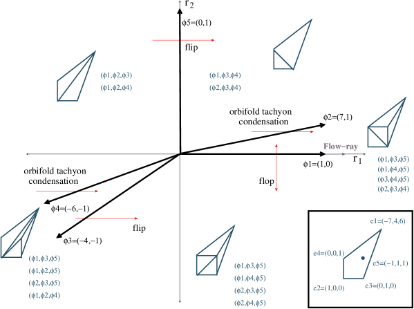
Figure 4: Phases of $Q=(1\ 7\ -4\ -6)$, with the toric subdivisions and corresponding coordinate charts in each phase, as well as the RG flow directions and the physics of each phase boundary.

The D-term equations (suppressing the gauge couplings) in this theory are

$$-D_{1} = |\phi_{1}|^{2}+7|\phi_{2}|^{2}-4|\phi_{3}|^{2}-6|\phi_{4}|^{2}-r_{1}=0\ ,$$

$$-D_{2} = |\phi_{2}|^{2}+|\phi_{5}|^{2}-|\phi_{3}|^{2}-|\phi_{4}|^{2}-r_{2}=0\ .$$ (50)

The three other D-terms obtained from different linear combinations of the two $U(1)$s are

$$-D_{2}^{\prime} = -D_{1}+7D_{2}=|\phi_{1}|^{2}+3|\phi_{3}|^{2}+|\phi_{4}|^{2}-7|\phi_{5}|^{2}-(r_{1}-7r_{2})=0\ ,$$

$$-D_{3}^{\prime} = -D_{1}+4D_{2}=|\phi_{1}|^{2}+3|\phi_{2}|^{2}-2|\phi_{4}|^{2}-4|\phi_{5}|^{2}-(r_{1}-4r_{2})=0\ ,$$ (51)

$$-D_{4}^{\prime} = -D_{1}+6D_{2}=|\phi_{1}|^{2}+|\phi_{2}|^{2}+2|\phi_{3}|^{2}-6|\phi_{5}|^{2}-(r_{1}-6r_{2})=0\ .$$

These D-terms give five phase boundaries in terms of rays drawn from the origin $(0,0)$ out through the points $\phi_{1}\equiv(1,0),\ \phi_{2}\equiv(7,1),\ \phi_{3}\equiv(-4,-1),\ \phi_{4}\equiv(-6,-1),\ \phi_{5}\equiv(0,1)$.

The phase structure of this theory, encapsulated in Figure 4, can be analyzed in the same way as in the previous case, so we will be brief here. The renormalization group flows in the GLSM are given by the 1-loop runnings of the two FI parameters $r_{a}$

$$r_{1}(\mu)=-{2\over 2\pi}\cdot\log{\mu\over\Lambda}\ ,\qquad\qquad r_{2}(\mu)=(0)\cdot\log{\mu\over\Lambda}+r_{2}^{(0)}\ .$$ (52)

Thus the parameter $r_{2}$ represents a marginal direction, and we have explicitly shown the value $r_{2}^{(0)}$ of the modulus. The RG flow of $r_{1}$ however forces $r_{1}\rightarrow\infty$ in the infrared. Thus the Flow-ray is the ray $(1,0)\equiv\phi_{1}$ in $r$-space (perpendicular to the $r_{2}$ direction). There are two convex hulls $\{\phi_{1},\phi_{2}\},\ \{\phi_{1},\phi_{3}\}$, adjoining the Flow-ray, so that there are two stable phases in this case, the $r_{a}$ satisfying $0<r_{2}<{1\over 7}r_{1}$ and ${1\over 4}r_{1}<r_{2}<0$ respectively. The ultraviolet of the theory, containing the ray $-F=(-1,0)$, is the phase $\{\phi_{4},\phi_{5}\}$ corresponding to the shrinking 2-sphere ${\mathbb{P}}^{1}_{-}$ with residual orbifold singularities. We can see that the nontrivial RG flows of the parameters $r_{1}-7r_{2}$ and $r_{1}-4r_{2}$ force all flowlines to cross these phase boundaries, thereby passing $into$ the phases $\{\phi_{1},\phi_{2}\}$ and $\{\phi_{1},\phi_{3}\}$ respectively.

Physically, the geometry of, say, phase $\{\phi_{1},\phi_{2}\}$ corresponds to the 2-cycle $\{e_{3},e_{4}\}$ and the 4-cycle $e_{5}$ blowing up simultaneously and expanding in time, separating the spaces described by the coordinate patches $\{\ (\phi_{3},\phi_{4},\phi_{5}),\ (\phi_{2},\phi_{3},\phi_{4}),\ (\phi_{1},\phi_{4},\phi_{5}),\ (\phi_{1},\phi_{3},\phi_{5})\ \}$, with the corresponding toric subdivision in Figure 4 showing the way these pieces of spacetime are glued together on the overlaps of their corresponding coordinate patches. Similarly we can describe the geometry of the topologically distinct phase $\{\phi_{1},\phi_{3}\}$. The blowup mode corresponding to the 2-cycle has size given by Kähler class $r_{2}$ which has no renormalization. This marginality of $r_{2}$ physically means that in the course of the decay, the geometry can end up anywhere on this 1-parameter moduli space. In fact, the modulus $r_{2}$ corresponds to a topology-changing flop transition interpolating between the two resolutions represented by these phases, as can be seen from the corresponding subdivisions in Figure 4. Thus we expect that the geometry will sometimes evolve precisely along the ray $r_{2}^{(0)}=r_{2}^{c},\ r_{1}\rightarrow\infty$, resulting in the supersymmetric conifold as a decay product. Indeed the vevs resulting from the nonzero value of $r_{1}$ Higgs the $U(1)^{2}$ down to $U(1)$, thus resulting in the singularity (using $D_{2}$)

$$\left\{|\phi_{2}|^{2}+|\phi_{5}|^{2}-|\phi_{3}|^{2}-|\phi_{4}|^{2}=0\right\}//U(1)\ ,$$ (53)

which is of course the supersymmetric conifold $Q=(\begin{array}[]{cccc}1&1&-1&-1\end{array})$. Since this is a real codimension-2 singularity in this infrared moduli space, we expect that this is an occasional decay product. Generically the geometry will end up in either of the two stable phases $\{\phi_{1},\phi_{2}\},\ \{\phi_{1},\phi_{3}\}$, corresponding to the small resolutions (related by a flop) of this residual singularity, obtained when $r_{2}>0$ and $r_{2}<0$ respectively, as can be seen from the collection of coordinate charts describing the two phases.
Here also, the two stable phases are less singular than any of the other phases.

Note that the conifold-like singularity $C(0;e_{1},e_{2},e_{4},e_{5})\equiv Q^{\prime}=(\begin{array}[]{cccc}1&3&-2&-4\end{array})$ also arises among the phases of this theory: this is of course an unstable singularity and the flip leading to its more stable resolution connects the phases $\{\phi_{3},\phi_{4}\}$ and $\{\phi_{1},\phi_{3}\}$. This is also a Type II singularity, consistent with the GSO projection.

3.3 Decays to $Y^{pq}$ spaces

Higher order unstable singularities include, besides the supersymmetric conifold, the supersymmetric $Y^{pq}$ spaces defined by $Q=(\begin{array}[]{cccc}p-q&p+q&-p&-p\end{array}),\ q<p$, ($p,q$ coprime), and $L^{a,b,c}$ spaces with $(\begin{array}[]{cccc}a&b&-c&-(a+b-c)\end{array}),c<a+b$, amidst the phases arising in their evolution (see Appendix C for a brief description of the phase structure of the $Y^{pq}$s).

A simple subfamily of the $Y^{pq}$s is defined by $Q=(\begin{array}[]{cccc}1&2p-1&-p&-p\end{array})$. This has the toric cone defined by $e_{5}=(-(2p-1),p,p),\ e_{2}=(1,0,0),\ e_{3}=(0,1,0),\ e_{4}=(0,0,1)$. For such a singularity to arise as a decay product in the phases of some higher order unstable singularity, its cone must exist as a subcone in the cone of the latter. If we restrict attention to singularities of the form $Q=(\begin{array}[]{cccc}1&n_{2}&-n_{3}&-n_{4}\end{array})$, then the point $e_{5}$ must be an interior point of the cone defined by $e_{1}=(-n_{2},n_{3},n_{4})$ and $e_{2},e_{3},e_{4}$, in particular lying in the interior of the orbifold subcone $C(0;e_{1},e_{3},e_{4})$. In other words, we have

$$e_{5}=(-(2p-1),p,p)=a(-n_{2},n_{3},n_{4})+b(0,1,0)+c(0,0,1)\ ,$$

$$\qquad\qquad\qquad\ 0<a,b,c<1\ ,\qquad a+b+c<1\ ,$$ (54)

the last condition expressing $e_{5}$ to be a tachyon of the orbifold subcone $C(0;e_{1},e_{3},e_{4})$. This then gives conditions on the $n_{i}$

$$(p-1)n_{2}<(2p-1)n_{3}<pn_{2}\ ,\qquad(p-1)n_{2}<(2p-1)n_{4}<pn_{2}\ ,\qquad 1+n_{2}<n_{3}+n_{4}\ .$$ (55)

Roughly speaking, this means that the affine hyperplane of the subcone $C(0;e_{1},e_{3},e_{4})$ must be appropriately tilted so as to encompass the lattice point $e_{5}$. This gives lower bound restrictions on the embedding unstable singularity, the order of the embedding singularity rapidly rising with $p$ due to these restrictions.

For example, consider the simplest such singularity $Y^{21}\equiv(\begin{array}[]{cccc}1&3&-2&-2\end{array})$. Then the above conditions give

$${n_{2}\over 3}<n_{3},n_{4}<{2n_{2}\over 3}\ ,\qquad 1+n_{2}<n_{3}+n_{4}\ ,$$ (56)

the first of which conditions automatically implies that the point $e_{6}=(-1,1,1)$ is also an interior point as can be checked by a simple calculation. This corresponds to the fact that one of the blowup modes of the $Y^{pq}$ singularities is the supersymmetric conifold (see Appendix C). One of the simplest unstable Type II singularities satisfying these conditions is $Q=(\begin{array}[]{cccc}1&17&-9&-11\end{array})$. Then we have $C(0;e_{1},e_{3},e_{4})\equiv{\mathbb{Z}}_{17}(1,8,-11)$, and

$$e_{5}=(-3,2,2)={1\over 17}(3e_{1}+7e_{3}+e_{4})\ ,\qquad e_{6}=(-1,1,1)={1\over 17}(e_{1}+8e_{3}+6e_{4})$$ (57)

corresponding to its GSO-preserved $j=3$ and $j=1$ twisted sector tachyons of R-charge $({3\over 17},{7\over 17},{1\over 17})$ and $({1\over 17},{8\over 17},{6\over 17})$ respectively.

Including say $e_{5}$ alone gives a 2-parameter system defined by

$$Q_{i}^{a}=\left(\begin{array}[]{ccccc}1&17&-9&-11&0\\ 0&3&-2&-2&1\\ \end{array}\right)\ ,$$ (58)

which can be analyzed along the same lines as before, resulting in the $Y^{21}$ space as an occasional decay product. Including both $e_{5}$ and $e_{6}$ gives a 3-parameter system with charge matrix

$$Q_{i}^{a}=\left(\begin{array}[]{cccccc}1&17&-9&-11&0&0\\ 0&3&-2&-2&1&0\\ 0&1&-1&-1&0&1\\ \end{array}\right)\ .$$ (59)

The Flow-ray for this system is $(1,0,0)\equiv\phi_{1}$. By analyzing the secondary fan using the general techniques outlined earlier (and described for a 3-tachyon system in unstable orbifolds in [6]), it can be seen that there are four phases adjoining the Flow-ray, which are the stable phases of this theory corresponding to the various resolutions involving $Y^{21}$ and the supersymmetric conifold contained as an interior blowup mode. It is straightforward to work out the details.

More generally, these techniques show that higher order unstable conifold singularities contain blowup modes giving rise to $L^{a,b,c}$ spaces amidst their stable phases.

4 Discussion

We have explored the phase structure of the nonsupersymmetric conifold-like singularities discussed initially in [4], exhibiting a cascade-like structure containing lower order conifold-like singularities including supersymmetric ones: this supplements the small resolutions studied in [4]. The structure is consistent with the Type II GSO projection obtained previously.

The GLSMs used here, as for unstable orbifolds, all have $(2,2)$ worldsheet supersymmetry, and have close connections with their topologically twisted versions, i.e. the corresponding A-models, so that various physical observables (in particular those preserving worldsheet supersymmetry) are protected along the RG flows here. However we note that the details of the RG evolution (and therefore also of time evolution) of the nonlinear sigma models (NLSMs) corresponding to these conifold-like geometries can be slightly different from the phase structure obtained here in the GLSM. For instance, while twisted sector tachyons (and their corresponding blowup modes) localized at the residual orbifold singularities on the 2-cycle loci have only logarithmic flows in the GLSM, on the same footing as the 2-cycle modes, they are relevant operators in the NLSMs with nontrivial anomalous dimensions. Thus in the NLSM (and in spacetime), the rate of evolution of a localized tachyon mode is expected to be higher than that of a 2-cycle mode, at least in the large volume limit where the 2-cycle evolution is slow. However although these details could be different, it seems reasonable, given worldsheet supersymmetry, to conjecture that the GLSM faithfully captures the phase structure and the evolution endpoints. A related issue is that the marginal directions orthogonal to the flow-ray preserved along the entire GLSM RG flow are only expected to coincide with corresponding flat directions arising at the $final$ IR endpoints in spacetime, which are supersymmetric as for orbifolds [5]. However in spacetime (with broken supersymmetry), it is not clear if there would be any corresponding exactly massless scalar fields during the course of time evolution. Presumably this is reconciled by taking into account the radiation effects present in spacetime but invisible in these (dissipative) RG analyses, which may also be related to string loop corrections (since the dilaton might be expected to turn on).

It is worth mentioning that the classical geometry analysis in [4] on obstructions to the 3-cycle (complex structure) deformation of these singularities due to their structure as quotients of the supersymmetric conifold suggests that there are no analogs of “strong” topology change and conifold transitions with nonperturbative light wrapped brane states here. From the GLSM point of view, the singular region where all $r_{a}$ vanish arises in the “middle” of the RG flow and is a transient intermediate state where the approximations in this paper are not reliable. It might be interesting to understand the structure of instanton corrections with a view to obtaining a deeper understanding of the physics of the singular region encoding the flip.

On a somewhat broader note, it might be interesting to understand and develop interconnections between renormalization group flows in generalizations of the GLSMs considered here (and the “space of physical theories” they describe) and Ricci flows in corresponding geometric systems. The fact that the GLSM RG trajectories in the conifold-like geometries here as well as those in [6] flow towards less singular geometries (smaller $N$ lattice volumes) suggests that there is a monotonically decreasing c-function-like geometric quantity here. Physically this seems analogous to the tachyon potential, or a height function on the “space of geometries”.

It would be interesting to understand D-brane dynamics in the context of such singularities. We expect that the quivers for these D-brane theories will be at least as rich as those for the $L^{a,b,c}$ spaces described in [13], and perhaps the knowledge of the phase structure of these theories developed here will be helpful in this regard. It is interesting to ask what these D-brane quivers (or possible duals) see as the manifestation of these instabilities.

Finally we make a few comments on compactifications of these (noncompact) conifold-like singularities. We expect that such a nonsupersymmetric conifold singularity can be embedded (classically) in an appropriate nonsupersymmetric orbifold of a Calabi-Yau that develops a localized supersymmetric conifold singularity, such that the quotienting action on the latter results in the nonsupersymmetric one. For quotient actions that are isolated, the Calabi-Yau only acquires discrete identifications so that the resulting quotient space “downstairs” is locally Calabi-Yau. While we expect that the low-lying singularities, i.e. small $n_{i}$, admit such locally supersymmetric compactifications, we note that the higher order ones may not. In fact there may be nontrivial constraints on the $n_{i}$ for the existence of such compactifications. In the noncompact case, we note that the early time semiclassical phase is a small resolution ${\mathbb{P}}^{1}_{-}$ of topology distinct from that of the late time small resolution ${\mathbb{P}}^{1}_{+}$ phase. We expect that both these phases, being semiclassical, admit descriptions as topologically distinct small resolutions in compact embeddings comprising orbifolds of appropriate Calabi-Yaus as described above. Thus one might think that the (intermediate) flip visible explicitly in the GLSM here persists in the compact context as well, where it would mediate mild time-dependent topology change of the ambient compact space, with changes in the intersection numbers of the various cycles of the geometry. However since in the compact context worldsheet RG techniques are subject to the strong constraints imposed by the c-theorem, it is not clear if our GLSM analysis here is reliable in gaining insight into the dynamics of compact versions of the flip transitions here (see e.g. [15] for related discussions in the context of string compactifications on Riemann surfaces). It would be desirable to obtain a deeper understanding of these compactifications [16] and their dynamics, perhaps implementing the quotient action on the Calabi-Yau directly in a spacetime description. From the latter perspective, the time dependence of the compact internal space would imply interesting time-dependent effects in the remaining 4-dimensional part of spacetime: for instance, in a simple FRW-cosmology-like setup, the 4D scale factor will evolve in accordance with the time dynamics of the internal space. It would be interesting to explore this here perhaps along the lines of [17].

Acknowledgments: I have benefitted from an early discussion with R. Gopakumar and from comments from S. Minwalla and D. Morrison on a draft.

Appendix A A review of ${\mathbb{C}}^{3}/{\mathbb{Z}}_{N}$ orbifolds: geometry and conformal field theory

In this section, we review some of the features [5] of the conformal field theory of ${\mathbb{C}}^{3}/{\mathbb{Z}}_{N}$ orbifold singularities, and the way they dovetail with the toric geometry description of these singularities. In particular, we will also review the correspondence between operators in the orbifold conformal field theory and subspaces in the $N$ lattice.

The spectrum of twisted sector string excitations in a ${\mathbb{C}}^{3}/{\mathbb{Z}}_{N}(k_{1},k_{2},k_{3})$ orbifold conformal field theory, classified using the representations of the ${\cal N}{=}2$ superconformal algebra, has a product-like structure (one for each of the three complex planes) giving eight chiral and anti-chiral rings in four conjugate pairs. A chiral ring twist field operator has the form $X_{j}=\prod_{i=1}^{3}\ X^{i}_{\{jk_{i}/N\}}=\prod_{i=1}^{3}\ \sigma_{\{jk_{i}/N\}}\ e^{i\{jk_{i}/N\}(H_{i}-{\bar{H}}_{i})}$, where $\sigma_{a}$ is the bosonic twist-$a$ field operator, while the $H_{i}$ are bosonized fermions. These correspond to relevant, marginal and irrelevant operators with worldsheet R-charges $R_{j}\equiv(\{{jk_{1}\over N}\},\{{jk_{2}\over N}\},\{{jk_{3}\over N}\})=\sum_{i}\{{jk_{i}\over N}\}$ and masses in spacetime given by $m_{j}^{2}={2\over\alpha^{\prime}}(R_{j}-1)$.

The geometry of such an orbifold can be recovered efficiently using its toric data. Let the toric cone of this orbifold be defined by the origin and lattice points $\alpha_{1},\alpha_{2},\alpha_{3}$ (see Figure 5): the points $\alpha_{i}$ define an affine hyperplane $\Delta$ passing through them. The volume of this cone $V(0;\alpha_{1},\alpha_{2},\alpha_{3})\equiv|{\rm det}(\alpha_{1},\alpha_{2},\alpha_{3})|=|\alpha_{1}\cdot\alpha_{2}\times\alpha_{3}|$ gives the order $N$ of the orbifold singularity. The specific structure of the orbifold represented by a toric cone $C(0;\alpha_{1},\alpha_{2},\alpha_{3})$ can be gleaned either using the Smith normal form algorithm [5], or equivalently by realizing relations between the lattice vectors $\alpha_{i}$ and any vector that is also itself contained in the $N$ lattice: e.g. we see that the cone defined by $\alpha_{1}=(N,-p,-q),\alpha_{2}=(0,1,0),\alpha_{3}=(0,0,1)$, corresponds to ${\mathbb{C}}^{3}/{\mathbb{Z}}_{N}(1,p,q)$ using the relation $(1,0,0)={1\over N}(\alpha_{1}+p\alpha_{2}+q\alpha_{3})$ with the lattice point $(1,0,0)$. Note that in general this only fixes the orbifold weights upto shifts by the order $N$.

There is a 1-1 correspondence between the chiral ring operators and points in the $N$ lattice toric cone of the orbifold. A given lattice point $P_{j}=(x_{j},y_{j},z_{j})$ can be mapped to a twisted sector chiral ring operator in the orbifold conformal field theory by realizing that this vector can expressed in the $\{\alpha_{1},\alpha_{2},\alpha_{3}\}$ basis as

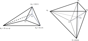
Figure 5: The ${\mathbb{C}}^{3}/{\mathbb{Z}}_{N}(1,p,q)$ orbifold toric fan, and tachyonic lattice points with their subdivisions.

$$(x_{j},y_{j},z_{j})=r_{1}\alpha_{1}+r_{2}\alpha_{2}+r_{3}\alpha_{3}\ .$$ (60)

If $r_{i}>0$, then $P_{j}$ is in the interior of the cone. This then corresponds to an operator $O_{j}$ with R-charge $R_{j}\equiv(r_{1},r_{2},r_{3})$. Conversely, it is possible to map an operator $O_{j}$ of given R-charge to a lattice point $P_{j}$. There are always lattice points lying “above” the affine hyperplane $\Delta$, corresponding to irrelevant operators: these have $R_{j}=\sum_{i}r_{i}>1$. Interior points lying $on$ $\Delta$ have $R_{j}=1$ and are marginal operators, while those “below” the hyperplane $\Delta$ have $R_{j}<1$ and correspond to tachyons. The toric cone of this orbifold can thus be subdivided by any of the tachyonic or marginal blowup modes (the irrelevant ones are unimportant from the physics point of view), giving rise to three residual subcones: these are potentially orbifold singularities again, unstable to tachyon condensation. For example, condensation of the tachyon $T=({1\over N},{p\over N},{q\over N})$ in the ${\mathbb{C}}^{3}/{\mathbb{Z}}_{N}(1,p,q)$ orbifold, corresponds to the subdivision of the cone $C(0;\alpha_{1},\alpha_{2},\alpha_{3})$ by the interior lattice point $T\equiv(1,0,0)$. From the GLSM point of view, this corresponds to RG flow of the single Fayet-Iliopoulos parameter in a GLSM with a $U(1)$ gauge group and charge matrix $Q=(\begin{array}[]{cccc}1&p&q&-N\end{array})$: this gives the resolved phase as the stable phase. Systems of multiple tachyons in orbifolds can be analyzed by appropriate generalizations of this GLSM [6], and generically exhibit flips amidst their phases.

A ${\mathbb{C}}^{3}/{\mathbb{Z}}_{N}(1,p,q)$ orbifold (Figure 5) is isolated if $p,q$ are coprime w.r.t. $N$: this is equivalent to the condition that there are no lattice points on the walls of the defining toric cone. For example, if $q,N$ have a common factor $n$ with $q=m_{1}n,\ N=m_{0}n$, then the $\{e_{1},e_{2}\}$ wall has the integral lattice point ${1\over n}(N,-p,-q)+\{{p\over n}\}(0,1,0)=(m_{0},-[{p\over n}],-m_{1})$. Similarly the $\{e_{1},e_{3}\}$ wall has integral lattice points if $p,N$ have common factors.

There is one further important issue raised by the GSO projection for these residual orbifold subcones and the lattice points in their interior. From the results of [5], we have that an orbifold ${\mathbb{C}}^{3}/{\mathbb{Z}}_{N}(k_{1},k_{2},k_{3})$ admits a Type II GSO projection if $\sum_{i}k_{i}=even$. In addition, this GSO projection acts nontrivially on the twisted sector operators, preserving only some states in each of the four independent chiral or anti-chiral rings of the orbifold conformal field theory. For example, the $j$-th twisted sector chiral ring operator $X_{j}$ with R-charge $R_{j}=(\{{jk_{1}\over N}\},\{{jk_{2}\over N}\},\{{jk_{3}\over N}\})$ is GSO-preserved iff

$$E_{j}=\sum_{i}\left[{jk_{i}\over N}\right]=odd\ .$$ (61)

It can be shown that under condensation of a GSO-preserved tachyon $T_{j}$, the GSO projection for the residual orbifolds and residual tachyons is consistent with this description. In other words, each of the three residual orbifolds admits a Type II GSO projection, and originally GSO-preserved residual tachyons continue to be GSO-preserved after condensation of a GSO-preserved tachyon for each of the three residual singularities.

Geometric terminal singularities arise if there is no Kähler blowup mode: i.e. there is no relevant or marginal chiral ring operator and no lattice point in the interior of the toric cone. However, a physical analysis of the system must include all possible tachyons in all rings, i.e. both Kähler and non-Kähler blowup modes. Then it turns out that there are no all-ring terminal singularities in Type II theories, while ${\mathbb{C}}^{3}/{\mathbb{Z}}_{2}(1,1,1)$ is the only terminal singularity (in Type 0 theories). Thus the endpoint of tachyon condensation in Type II theories is smooth.

Appendix B Phase structure of $Y^{pq}$ singularities

The $Y^{pq}$ singularities are defined by $Q=(\begin{array}[]{cccc}p-q&p+q&-p&-p\end{array})$, with $q<p$ and $p,q$ coprime. More general noncompact Calabi-Yau spaces include the $L^{a,b,c}$s which are defined by $Q=(\begin{array}[]{cccc}a&b&-c&-d\end{array})$, with $\sum_{i}Q_{i}=0$. Since $\sum_{i}Q_{i}=0$ for all these, the $e_{i}$ defining the cone are coplanar, and the singularities admit a Type II GSO projection as expected. There is no RG flow for Fayet-Iliopoulos parameters in the corresponding GLSM and all phases are on equal footing, defining distinct resolutions of the singularity.

For example, the singularity $Y^{32}$, defined by the charge matrix $Q=(\begin{array}[]{cccc}1&5&-3&-3\end{array})$, can be represented by the toric cone with $e_{1}=(-5,3,3),\ e_{2}=(1,0,0),\ e_{3}=(0,1,0),\ e_{4}=(0,0,1)$. There are two interior lattice points, $e_{5}=(-1,1,1)={e_{1}+2e_{2}\over 3}$ and $e_{6}=(-3,2,2)={2e_{1}+e_{2}\over 3}$, lying on the $\{e_{1},e_{2}\}$ plane. The subcones $C(0;e_{5},e_{2},e_{3},e_{4})$ and $C(0;e_{6},e_{2},e_{3},e_{4})$ define the lower order singularities corresponding to the supersymmetric conifold $Q=(\begin{array}[]{cccc}1&1&-1&-1\end{array})$ and $Y^{21}\equiv Q=(\begin{array}[]{cccc}1&3&-2&-2\end{array})$.

Considering GLSMs that incorporate these interior lattice points gives the full phase structure of these spaces. For instance, including say the lattice point $e_{5}$ alone gives a 2-parameter GLSM with charge matrix

$$Q_{i}^{a}=\left(\begin{array}[]{ccccc}1&5&-3&-3&0\\ 0&1&-1&-1&1\\ \end{array}\right)\ ,$$ (62)

with two FI parameters that do not run. Since two phase boundaries $\phi_{3}=\phi_{4}=(-3,-1)$ coincide, we obtain four phases here instead of five as in the Examples in Sec. 3. We could also use the relation $e_{5}={1\over 5}(e_{1}+2e_{3}+2e_{4})$ stemming from $e_{5}\in C(0;e_{1},e_{3},e_{4})$ to define $Q_{i}^{a}$, obtaining equivalent phases. Including both $e_{5}$ and $e_{6}$ gives a 3-parameter GLSM describing the complete resolution of the singularity.

The higher order $Y^{pq}$s contain multiple interior points corresponding to some or all of the lower order $Y^{pq}$s. Analyzing their phase structure using a multiple parameter GLSM exhibits phases corresponding to various partial/complete resolutions involving lower order $Y^{pq}$ spaces.

Similarly we can see that the higher order $L^{a,b,c}$ spaces typically contain blowup modes giving lower order $L^{a,b,c}$s in their partial resolutions.

References

- [1] E. Martinec, “Defects, decay and dissipated states”, [hep-th/0210231].
- [2] M. Headrick, S. Minwalla, T. Takayanagi, “Closed string tachyon condensation: an overview”, [hep-th/0405064].
- [3] E. Witten, “Phases of theories in two dimensions”, [hep-th/9301042].
- [4] K. Narayan, “Closed string tachyons, flips and conifolds”, [hep-th/0510104].
- [5] David R. Morrison, K. Narayan, M. Ronen Plesser, “Localized tachyons in ”, [hep-th/0406039].
- [6] David R. Morrison, K. Narayan, “On tachyons, gauged linear sigma models and flip transitions”, [hep-th/0412337].
- [7] T. Sarkar, “On localized tachyon condensation in and ”, [hep-th/0407070].
- [8] D. Freedman, M. Headrick, A. Lawrence, “On closed string tachyon dynamics”, [hep-th/0510126].
- [9] T. Suyama, “Closed string tachyon condensation in supercritical strings and RG flows”, [hep-th/0510174].
- [10] D. R. Morrison, M. R. Plesser, “Summing the instantons: quantum cohomology and mirror symmetry in toric varieties”, [hep-th/9412236].
- [11] B. R. Greene, “String theory on Calabi-Yau manifolds”, [hep-th/9702155].
- [12] D. Martelli, J. Sparks, “Toric geometry, Sasaki Einstein manifolds and a new infinite family of AdS/CFT duals”, [hep-th/0411238].
- [13] S. Franco, A. Hanany, D. Martelli, J. Sparks, D. Vegh, B. Wecht, “Gauge theories from toric geometry and brane tilings”, [hep-th/0505211].
- [14] E. Witten, in Quantum fields and strings: a course for mathematicians, see, e.g., Lecture 12 at http://www.cgtp.duke.edu/QFT/spring/.
- [15] A. Adams, X. Liu, J. McGreevy, A. Saltman, E. Silverstein, “Things fall apart: topology change from winding tachyons”, [hep-th/0502021].
- [16] Work in progress.
- [17] K. Dasgupta, P. Chen, K. Narayan, M. Shmakova, M. Zagermann, “Brane inflation, solitons and cosmological solutions: I”, [hep-th/0501185].