We study the expectation values of Wilson-loop operators with the insertions of local operators $Z^{J}$ and $\overline{Z}^{J}$ for large $J$ from the bulk viewpoint of AdS/CFT correspondence. Classical solutions of strings attached to such deformed Wilson loops at the conformal boundary are constructed and are applied to the computation of Wilson-loop expectation values. We argue that in order to have such solutions for general insertions at finite positions in the base spacetime of the gauge theory, it is crucial to interpret the holographic correspondence in the semi-classical picture as a tunneling phenomenon, as has been previously established for holographic computations of correlators of BMN operators. This also requires to use the Euclideanized AdS background and Euclidean super Yang-Mills theory.

1. Introduction

In the applications of the conjectured AdS/CFT (or gravity/gauge) correspondence [1, 2], Wilson-loop expectation values have been a focus of much interest. Besides their role as an important probe for studying phase structures of gauge theories, the Wilson-loop operators have long been regarded as a clue to possible string picture for gauge theories. With the advent of the AdS/CFT correspondence, Wilson loops in general can be associated with the world sheet of strings in the bulk AdS spacetime, in such a way that the boundary of the string world sheets coincides with the locus of a given Wilson loop located on a holographic screen at the conformal boundary of the AdS background. Using this picture initiated in [3], a lot of interesting results have been reported. Most of such results obtained from the viewpoint of bulk string theory should be regarded as predictions of the AdS/CFT correspondence, and direct checks of corresponding results on the gauge-theory side have been difficult because they usually require genuine nonperturbative calculations. In certain special cases, such as circular (or straight-line) loops [4, 5] which can be constrained by (super)conformal symmetries, some pieces of nontrivial evidence for the agreement of both sides have been obtained. For example, it has been shown [6, 7, 8] that a ladder-graph approximation gives results which are consistent with predictions from the string picture in the bulk. It is important to extend such correspondence to other cases.

A first extension to be considered along this line would be various small deformations of loops from circle, although it is still difficult to perform such calculation on the gauge-theory side, since we cannot expect that ladder-type approximations continue to be valid for general small deformations. Another interesting case would be those with various insertions of local operators along the Wilson line. In particular, we can consider insertions of local operators with large R-charge angular momentum $J$ such as $Z(x)^{J}$ and their cousins, “spin-chain operators”. Such operators can preserve covariance under an SL(2, R) part of conformal transformations.

In a recent paper [11], a nice discussion of such Wilson loops has been given. On the bulk side, the authors discussed the spectrum of strings in the large $J$ limit. The insertions of the local operators are interpreted as nonzero $S^{5}$-angular momentum density on the world sheet which is essentially concentrated at the center of the AdS₅ background in their treatment. The special role of the AdS center follows from a familiar discussion of the BMN limit [12] corresponding to $Z^{J}$, while the (doubled) Wilson lines are still located at the conformal boundary without any deformation. The absence of deformation on the conformal boundary has been interpreted as signifying the situation where the positions of operator insertions are sent to infinity with an infinitely large loop.

In the context of bulk string picture, however, it is clearly more natural to consider string world sheets with nontrivial deformations corresponding to the insertions of local composite operators at generic finite points on the conformal boundary. We would then be able to directly evaluate the expectation values for arbitrary circular loops using such string solutions by following the standard bulk interpretation of Wilson-loop expectation values. The purpose of the present note is to demonstrate how to achieve such a picture in a simplest nontrivial setting and to give some remarks relevant to this question, in hope of providing a basis for further systematic investigations of Wilson-loop expectation values with more complicated configurations of local operator insertions. In particular, we will point out that a ‘tunneling’ picture which has been developed in [13, 14] in order to reconcile the BMN limit with the spacetime holographic picture is crucial for this purpose. This approach has led to a natural prescription [15] for a holographic correspondence between OPE coefficients of the conformal gauge theory to a particular 3-point vertex of string-field theory. Establishing such correspondence beyond mere comparison of the spectrum has been difficult in the usual approach which does not take into account the tunneling picture.

2. Tunneling picture and bulk string solutions

The Wilson-loop operator we consider is

$$W[C;\vec{x}_{+},\vec{x}_{-}]={\rm Tr}\Big{[}{\cal P}\exp\Big{(}\oint_{C}ds[iA_{\mu}(\vec{x}(s))\dot{x}^{\mu}+\sqrt{(\dot{\vec{x}})^{2}}\phi^{i}(\vec{x}(s))\theta^{i}]\Big{)}Z(\vec{x}(s_{1}))^{J}\overline{Z}(\vec{x}(s_{2}))^{J}\Big{]}$$ (1)

where $\vec{x}_{+}=\vec{x}(s_{1}),\,\vec{x}_{-}=\vec{x}(s_{2})$ are the positions of insertions and the contour $C$ is assumed to be a circle. We denote by $\vec{x}=\{x^{\mu}\}$ the 4-dimensional base spacetime coordinates. Other notations are standard. For simplicity, we assume that the direction of the unit vector $\theta^{i}$ along the $S^{5}$ is fixed to be the 4-th direction, $\phi^{i}\theta^{i}=\phi^{4}$ and that the direction of the angular momentum is in the $5$-$6$ plane, $Z=(\phi_{5}+i\phi_{6})/\sqrt{2}$. If we wish to study the behavior of the vacuum expectation value of this operator from the viewpoint of string theory in the bulk, the first task is to obtain an appropriate classical string configuration such that, as we approach the conformal boundary, it reduces to the circle $C$ with the momentum density along $C$ being concentrated at the positions of insertions. We choose the Polyakov-type action in the conformal gauge for world-sheet parametrization. Also for the target spacetime, we use the Poincaré coordinates for the AdS part with the metric

$$ds^{2}=R^{2}\Big{[}\frac{dz^{2}+d\vec{x}^{2}}{z^{2}}+\cos^{2}\theta(d\psi)^{2}+(d\theta)^{2}+\sin^{2}\theta d\tilde{\Omega}_{3}^{2}\Big{]}.$$ (2)

For the $S^{5}$ part, the 4-th direction pointing toward the north pole corresponds to $\theta={\pi/2}$ and the angle in the 5-6 plane at $\theta=0$ is $\psi$. The angular momentum along $\psi$ is then

$$J=\frac{R^{2}}{2\pi\alpha^{\prime}}\int d\sigma\cos^{2}\theta(\tau,\sigma)\dot{\psi}(\tau,\sigma).$$ (3)

Assume that the world-sheet time coordinate $\tau$ is chosen such that $\psi(\tau,\sigma)=\tau$. The equation of motion then requires that $\theta$ is $\tau$-independent. The density of the angular momentum with respect to $\sigma$ cannot exceed a finite constant $R^{2}/2\pi\alpha^{\prime}$. In order for the R-charge angular momentum to be localized with respect to the target spacetime, the range of $\sigma$ where $\cos\theta\sim 1,\vec{x}{\,{}^{\prime}}\sim 0,z^{\prime}\sim 0$ are satisfied must be infinitely large. For the $S^{5}$ part, the solution satisfying the criterion is easily found as in [11] to be

$$(\cos\theta,\psi)=(\tanh\sigma,\tau)$$ (4)

which also satisfies the Virasoro constraint in the form $(\dot{\psi})^{2}\cos^{2}\theta+(\theta^{\prime})^{2}=1,\,\,\dot{\psi}\psi^{\prime}\cos^{2}\theta+\dot{\theta}\theta^{\prime}=0.$ The region where the R-charge momentum is localized is where $\sigma\rightarrow\infty$. Thus, in the limit of large $\sigma$, the AdS coordinates must also be constant with respect to $\sigma$ at least when we consider the near-boundary region $z\sim 0$. Hence the Virasoro-Hamiltonian constraint in this region reduces to

$$\frac{\dot{z}^{2}+\dot{\vec{x}}^{2}}{z^{2}}+1=0.$$ (5)

This shows that for the existence of real solution, we have to require at least that $\dot{\vec{x}}$ is timelike. The equation of motion $\partial_{\tau}\Big{(}{\partial_{\tau}\vec{x}\over z^{2}}\Big{)}-\partial_{\sigma}\Big{(}{\partial_{\sigma}\vec{x}\over z^{2}}\Big{)}=0$ for $\vec{x}$ reduces, under the same condition, to $\dot{\vec{x}}/z^{2}=$ constant. We choose the scale of this integration constant by introducing a parameter $\ell$ such that $\dot{\vec{x}}^{2}/z^{4}=-\ell^{-2}$. However, we then have always $z^{2}\geq\ell^{2}$ since (5) is now equivalent to $\ell^{2}\dot{z}^{2}=z^{2}(z^{2}-\ell^{2})$. Since we are seeking for a string configuration of which the deformation corresponding to local operator insertions reaches the conformal boundary $z=0$, this is not acceptable. Hence, there exists no desired classical solution which reaches the conformal boundary even if we assume that the loop $C$ extends in the time-like direction. The situation [13, 14] is the same as in the usual formulation of the BMN limit for which it is not possible to directly apply the GKPW prescription for the same reason as we encounter here that the pp-wave trajectory with Lorentzian metric does not reach the conformal boundary. Hence, if we remain in the Lorentzian approaches such as in [11], we cannot achieve the desired picture.

The resolution of this puzzle is quite simple. We would like to refer the reader to [13, 14] for detailed discussions on this matter. In essence, we have to take into account that, from the viewpoint of semi-classical approximation, the holographic correspondence between bulk and conformal boundary is actually a tunneling phenomenon as could be inferred from the beginning of AdS/CFT correspondence embodied in the famous GKPW relation. Namely, we have to study the tunneling region $z^{2}(z^{2}-\ell^{2})\leq 0$. As is familiar in elementary quantum mechanics, we perform the Wick rotation $\tau\rightarrow-i\tau$ for the world-sheet time. We are then forced to consider Euclideanized AdS (EAdS) by assuming that $\vec{x}$ is now a 4-vector with Euclidean signature, in order to keep the relative sign between $z^{4}$ and $z^{2}\ell^{2}$ against the Wick rotation of the world-sheet time coordinate. Of course, if we started from a loop extending to space-like directions, only the Wick rotation with respect to $\tau$ would have been sufficient. However, when we consider the light-cone quantization of strings around the classical solution, the Wick rotation with respect to the target time direction would be very important irrespectively of the directions of the loop.

The Hamiltonian constraint now reduces to $\ell^{2}\dot{z}^{2}=z^{2}(\ell^{2}-z^{2})$, and the solution of the equation of motion is obtained as

$$z=\ell/\cosh\tau,\quad x_{4}=\ell\tanh\tau$$ (6)

which is nothing but a semi-circle $z^{2}+x_{4}^{2}=\ell^{2}$ in the two-dimensional section $(z,x_{4})$ and reaches the conformal boundary as $\tau\rightarrow\pm\infty$. We have chosen a trajectory lying in the 4-th direction of the EAdS spacetime. Note that the integration constant $\ell$ gives the distance $|\vec{x}_{+}-\vec{x}_{-}|=2\ell$ between the two local operator insertions on the boundary. It should also be noted that as a consequence of the above Wick rotation we have to rotate the angle coordinate along the 5-6 plane simultaneously as $\psi\rightarrow-i\psi$ to keep the value of R-charge angular momentum $J$ intact. Thus the 10-dimensional spacetime as a whole is of Lorentzian signature effectively. This is why we can still perform a Penrose-type limit in the tunneling picture. Eq.(6) is the same geodesic trajectory as the one used for discussing the correlators of the BMN operators and the associated ‘holographic’ string field theory [13, 15].

It is now evident that in order to have the world-sheet configuration corresponding to our Wilson-loop operator with local-operator insertions we have to rely on the tunneling picture. As in the case [13] of the BMN limit, the world-sheet time variable $\tau$ in (6) can be identified with the Euclidean time parameter $\tau$ of the global coordinates for EAdS background, $R^{2}[\cosh^{2}\rho(d\tau)^{2}+(d\rho)^{2}+\sinh^{2}\rho d\Omega_{3}^{2}]$ in terms of which the trajectory is nothing but the geodesic at $\rho=0$ which does reach the boundary in the limit of large $|\tau|$. The full string world-sheet will be described as a trajectory of an open string propagating from boundary to boundary such that the position of localized R-charge momentum traverses along this geodesic of the EAdS background. The desired solution can be easily obtained by going to the global EAdS metric and then return again to the Poincaré metric. In the case of straight-line Wilson loop, the solution in the global EAdS metric is in fact related to the solution discussed in [11] by our Wick rotation.

Choosing the circle $C$ on the boundary in the $x_{3}$-$x_{4}$ plane and the points of the insertions on the $x_{4}$ axis, we find that the full world sheet is described by two patches designated by suffix $\pm$, given as

$$(z(\tau,\sigma),x_{3}(\tau,\sigma),x_{4}(\tau,\sigma))_{\pm}$$

$$=\ell(\frac{\sinh\sigma}{\cosh\sigma\cosh\tau\pm\alpha},\pm\frac{\sqrt{1-\alpha^{2}}}{\cosh\sigma\cosh\tau\pm\alpha},\frac{\cosh\sigma\sinh\tau}{\cosh\sigma\cosh\tau\pm\alpha}).$$ (7)

In addition to the integration variable $\ell$ appeared already to describe the distance of insertion points, we introduced another parameter $\alpha$ which gives the radius, $r=\ell/\sqrt{1-\alpha^{2}}$, of the circle $C$ for a given $\ell$. As a matter of course, solutions with circles of different sizes on the conformal boundary are related by conformal transformations in the bulk EAdS background. For our later purpose, it is most convenient to keep these two integration constants explicitly. The ranges of the world-sheet coordinates are $0\leq\sigma\leq\infty$ and $-\infty\leq\tau\leq\infty$ for both patches. The trajectory (6), along which the R-charge angular momentum is concentrated and the two patches are sewn together, corresponds to the limit $\sigma\rightarrow\infty$ in conformity with the above discussion of localized angular momentum.

On the other hand, the limit $\sigma\rightarrow 0$ gives

$$(z(\tau,0),x_{3}(\tau,0),x_{4}(\tau,0))_{\pm}=\ell(0,\pm\frac{\sqrt{1-\alpha^{2}}}{\cosh\tau\pm\alpha},\frac{\sinh\tau}{\cosh\tau\pm\alpha})$$ (8)

which corresponds to the circle $C$ on the boundary whose center is located on the $x_{3}$ axis. The points of local operator insertions are $\vec{x}_{\pm}=\ell(0,0,\pm 1)$, as we obtain by taking the limits $\tau\rightarrow\pm\infty$, respectively, in either of these expressions ($\sigma=0$ or $\sigma\rightarrow\infty$). For the $S^{5}$ part, we can adopt the same form as (4) with the understanding of a double Wick rotation.

Figs. 1-3 exhibit the equal-$\tau$ and-$\sigma$ lines on the full world sheet with respect to the bulk target space. In particular, in the case of the straight-line loop ($\alpha=1$, Fig. 3), the two patches with signs $\pm$ correspond to the regions $z^{2}+x_{4}^{2}\leq\ell^{2}$ or $z^{2}+x_{4}^{2}\geq\ell^{2}$, respectively, and are related to each other by an inversion transformation $(z,x_{4})\rightarrow\ell^{2}(z/(z^{2}+x_{4}^{2}),x_{4}/(z^{2}+x_{4}^{2}))$. If we wished and did not insist on the conformal gauge, we could have represented the above solution using a single patch. In fact, the solution with $\alpha=1$ can equivalently be expressed using complex coordinates both for world sheet and target space as

$$\tau+i\tilde{\theta}=\ln i{x_{4}+\ell+iz\over x_{4}-\ell+iz},$$ (9)

where $\tilde{\theta}$ is related to $\sigma$ by $\tanh\sigma=\cos\tilde{\theta}$. The two patches correspond to $-\pi/2\leq\tilde{\theta}\leq 0$ and $0\leq\tilde{\theta}\leq\pi/2$. The solution with other values of $\alpha$ can of course be obtained by conformal transformation in the target space. This form is very suggestive, since it strikingly resembles to similar expressions in the light-cone string theory in flat spacetime. It might be worthwhile to elaborate this form further in a direction, say, of extending it to cases with multi-point insertions of local operators. For the purpose of the present note, however, we will use the above two-patch representation.

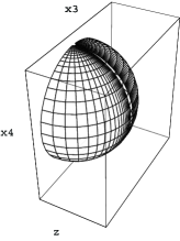
Fig. 1: The equal $\tau$-$\sigma$ curves on the full world sheet for the case of the smallest (with fixed $\ell$) loop $\alpha=0$.

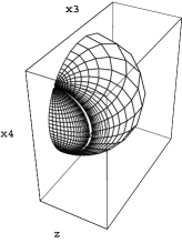
Fig. 2: The equal $\tau$-$\sigma$ curves on the full world sheet for a generic loop $0<\alpha<1$.

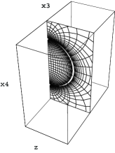
Fig. 3: The equal $\tau$-$\sigma$ curves on the full world sheet for the straight-line loop $\alpha=1$.

The total R-charge angular momentum carried by this solution is

$$J=\frac{R^{2}}{\pi\alpha^{\prime}}\int_{0}^{\infty}d\sigma\tanh^{2}\sigma,$$ (10)

which is infinite. Note that elimination of factor 2 in the prefactor before the integral is due to the presence of two patches. Thus, we have to actually introduce a cutoff for $\sigma\leq\sigma_{\Lambda}$ with a sufficiently large $\sigma_{\Lambda}\gg 1$, so that the angular momentum is now given as $J\sim R^{2}(\sigma_{\Lambda}-1)/\pi\alpha^{\prime}+O({\rm e}^{-2\sigma_{\Lambda}})$. With regard to the dependence on $J$, our treatment will be exact up to nonperturbative exponential corrections $O({\rm e}^{-2\pi\alpha^{\prime}J/R^{2}})$ which can be ignored in the power series expansion in $1/J$ within our semi-classical approximation.

3. Computing the Wilson-loop expectation value

Our next task is to evaluate the value of an appropriate classical string action functional for this configuration. We have adopted the Polyakov-type action for the bulk world sheet and are interpreting the process as a scattering event of an open string on the world sheet from $\tau=-\infty$ to $\tau=\infty$ for the given conserved R-charge angular momentum $J$. Thus we should consider the Routhian after a Legendre transformation with respect to $\psi$,

$$S_{bulk}=\frac{R^{2}}{4\pi\alpha^{\prime}}\int d\tau d\sigma\Big{[}\frac{1}{z^{2}}\Big{(}(\dot{z})^{2}+(z^{\prime})^{2}+(\dot{\vec{x}})^{2}+(\vec{x}^{\prime})^{2}\Big{)}+(\dot{\theta})^{2}+(\theta^{\prime})^{2}$$

$$\hskip 113.81102pt-\cos^{2}\theta\Big{(}(\dot{\psi})^{2}+(\psi^{\prime})^{2}\Big{)}-{4\pi\alpha^{\prime}\over R^{2}}\Pi_{\psi}\dot{\psi}\Big{]}$$ (11)

with $\Pi_{\psi}=-R^{2}\dot{\psi}\cos^{2}\theta/2\pi\alpha^{\prime}$ being the $\psi$-momentum. The minus sign of the $\psi$-part comes from the Wick rotation. Since the world-sheet has a boundary, the action functional is subject to ambiguity of boundary terms. We follow the argument of ref.[5] which demands that the total action should be a functional of momentum in the radial direction of the AdS part, with respect to the dependence on the boundary. This requirement does not yet uniquely fix the choice of the boundary term, since they are not in general invariant under canonical transformations. One natural criterion for the choice of the variable is that the momentum should behave in a well-defined manner as we approach the boundary. This criterion is not satisfied if we choose $z$, since the radial momentum $\Pi_{z}=R^{2}\dot{z}/2\pi\alpha^{\prime}z^{2}$ for the above solution is not well-defined at $z=0$, corresponding to $\sigma=0$. Instead of $z$, we choose $u=1/z$ since $\Pi_{u}=R^{2}\dot{u}/2\pi\alpha^{\prime}u^{2}$ behaves well there. These two different choices actually lead to boundary contributions with opposite signs. Thus the boundary action we adopt is

$$S_{boundary}=\frac{R^{2}}{2\pi\alpha^{\prime}}\oint_{boundary}\Big{(}d\tau\frac{u^{\prime}}{u}-d\sigma\frac{\dot{u}}{u}\Big{)}.$$ (12)

Then the expectation value of the Wilson operator (1) is essentially ${\rm e}^{-S_{bulk}-S_{boundary}}$ up to a possible normalization factor, which should not depend on the spacetime configuration of the loop $C$ and the positions $\vec{x}_{\pm}$ of insertions provided that the string action captures the gauge-theory dynamics of Wilson loops appropriately.

3.1 Regularization I

To carry out a well-defined evaluation of this action integral, we have to introduce a definite regularization scheme which controls possible infinities arising at least near the boundary region $z\sim 0$ corresponding to small $\sigma$ and/or large $\tau$. The simplest conceivable prescription is to introduce two cutoff parameters $\sigma_{0}$ and $\epsilon$ on the world sheet such that

$$\sigma\geq\sigma_{0},\quad\cosh\tau\leq\frac{\ell}{\epsilon}$$ (13)

and take the limits $\sigma_{0}\rightarrow 0,\epsilon\rightarrow 0$ afterward. The second condition amounts to setting a lower bound for the radial coordinate $z$ in the target space at the points of insertions for sufficiently large $\sigma$, $\lim_{\sigma_{\Lambda}\rightarrow\infty}z(\sigma_{\Lambda},\tau)\geq\epsilon.$ In the case of local operators, this is a standard short-distance cutoff in applying the GKPW relation. We assume that both the bulk and boundary actions should be computed for the same finite rectangular region defined by these cutoff conditions (13). For the cutoff $\sigma_{\Lambda}$ associated with large R-charge angular momentum, it is not necessary to introduce any boundary term.

Using the Virasoro condition

$$\frac{1}{z^{2}}(\dot{z}^{2}-(z^{\prime})^{2}+\dot{\vec{x}}^{2}-(\vec{x}^{\prime})^{2})=1=-\dot{\theta}^{2}+(\theta^{\prime})^{2}+\cos^{2}\theta((\dot{\psi})^{2}-(\psi^{\prime})^{2})$$ (14)

satisfied by the above solution and also a part of the equations of motion, the bulk action is evaluated to be

$$S_{bulk}=\frac{R^{2}}{\pi\alpha^{\prime}}\int_{-\tau(\epsilon)}^{\tau(\epsilon)}d\tau\int_{\sigma_{0}}^{\sigma_{\Lambda}}d\sigma\frac{\dot{z}^{2}+\dot{\vec{x}}^{2}}{z^{2}}=\frac{2R^{2}}{\pi\alpha^{\prime}}\int^{\tau(\epsilon)}_{0}d\tau(\sigma-\coth\sigma)\Big{|}^{\sigma_{\Lambda}}_{\sigma_{0}},$$ (15)

with $\tau(\epsilon)\sim\log(2\ell/\epsilon)$ being the upper bound for $|\tau|$ determined by (13). Because of the conformal isometry, the bulk action is independent of the radius $r$ of the circle, except for possible implicit dependence through the cutoff prescription. The boundary action is equal to

$$S_{boundary}=\frac{R^{2}}{\pi\alpha^{\prime}}\Big{[}\int_{0}^{\tau(\epsilon)}d\tau\Big{(}-2\coth\sigma_{0}+\frac{\sinh\sigma_{0}\cosh\tau}{\cosh\sigma_{0}\cosh\tau+\alpha}+\frac{\sinh\sigma_{0}\cosh\tau}{\cosh\sigma_{0}\cosh\tau-\alpha}\Big{)}$$

$$-\int_{\sigma_{0}}^{\sigma_{\Lambda}}d\sigma\Big{(}\frac{\cosh\sigma\sinh\tau(\epsilon)}{\cosh\sigma\cosh\tau(\epsilon)+\alpha}+\frac{\cosh\sigma\sinh\tau(\epsilon)}{\cosh\sigma\cosh\tau(\epsilon)-\alpha}\Big{)}\Big{]}.$$ (16)

The contribution of the first term $-2\coth\sigma_{0}$ in the first brace just cancels the same but opposite contribution from the second term at $\sigma=\sigma_{0}\rightarrow 0$ of the bulk action. Therefore, the total action is given, in the limit where the cutoff parameters must be finally set, by

$$S_{total}\equiv S_{bulk}+S_{boundary}=2J\log\frac{2\ell}{\epsilon}-2J-\frac{2R^{2}}{\pi\alpha^{\prime}}$$

$$-\frac{R^{2}}{\pi\alpha^{\prime}}\sigma_{0}\frac{2\alpha}{\sqrt{\cosh^{2}\sigma_{0}-\alpha^{2}}}\Big{(}\arctan\frac{\cosh\sigma_{0}-\alpha}{\sqrt{\cosh^{2}\sigma_{0}-\alpha^{2}}}-\arctan\frac{\cosh\sigma_{0}+\alpha}{\sqrt{\cosh^{2}\sigma_{0}-\alpha^{2}}}\Big{)}.$$ (17)

Note that we have still kept the small cutoff parameter $\sigma_{0}\ll 1$ here, since the last term has a rather subtle behavior depending on the parameter $\alpha$. When $\alpha<1$, this reduces in the limit $\sigma_{0}\rightarrow 0$ to

$$S_{total}\Big{|}_{\alpha<1}=2J\log\frac{2\ell}{\epsilon}-2J-\frac{2R^{2}}{\pi\alpha^{\prime}}.$$ (18)

The case $\alpha=1$ of the straight-line Wilson loop, however, is special: We obtain

$$S_{total}\Big{|}_{\alpha=1}=2J\log\frac{2\ell}{\epsilon}+\frac{R^{2}}{\alpha^{\prime}}-2J-\frac{2R^{2}}{\pi\alpha^{\prime}}.$$ (19)

The additional finite piece $R^{2}/\alpha^{\prime}$ in this result comes from the $(-)$ patch corresponding to the second term in the brace of (17) which is singular when $\alpha=1$.

Let us now discuss the meaning of these results. The dependence $dS_{total}/d(2\ell)=2J/2\ell$ on the distance $2\ell$ of the inserted local fields $Z^{J}$ and $\overline{Z}^{J}$ shows the correct scaling behavior as it should be by the conformal covariance property [11] of Wilson-loop operators of the type being treated here. On the other hand, the dependence on the loop-scale parameter $\alpha$ takes the form

$$S_{total}\Big{|}_{\alpha=1}-S_{total}\Big{|}_{\alpha<1}=\frac{R^{2}}{\alpha^{\prime}}.$$ (20)

This behavior is the same as in the case without local-operator insertions.

On the gauge-theory side, as argued in [7] for the case of ordinary circular Wilson loops without local operator insertions, the relation (20) can be interpreted as arising from an anomaly associated with the inversion conformal transformation between a finite circle and a straight line. Their argument seems go through to the case with local operator insertions. This is consistent with the ladder-graph approximation in the limit $R^{4}/(\alpha^{\prime})^{2}\gg 1$, since we can easily check that the contribution of ladder-rainbow graphs which take into account a planar set of the propagators of scalar ($\phi_{4}$) and gauge fields directly connecting points along the loop is nonzero only for the case of finite circle $\alpha<1$ and is proportional, apart from a power-behaving prefactor, to

$$I_{1}(\sqrt{g^{2}N}\frac{s}{2\pi})I_{1}(\sqrt{g^{2}N}\frac{2\pi-s}{2\pi})\rightarrow{\rm e}^{\sqrt{g^{2}N}},$$ (21)

using the same notation ($R^{4}/(\alpha^{\prime})^{2}=g^{2}N\gg 1$) as in the reference [8]. The new parameter $s\,\,(0<s<2\pi)$ denotes the coordinate length between two local operator insertions measured along the Wilson loop of total length $2\pi$. Thus the ratio of the case of finite circles to that of straight line agrees with (20). The ladder approximation is also consistent with the dependence on $\ell$. The validity of such an approximation has not been justified from first principle, but is not unreasonable in view of remaining supersymmetry for this type of deformation [16]. For a discussion related to supersymmetry of the Wilson loops of our type, we refer the reader to [11, 17].

The dependence on the short-distance cutoff parameter $\epsilon$ must be removed by wave-function renormalization of our Wilson loop operator as usual. On the other hand, it is not entirely clear whether we can put any universal meaning on the remaining finite contribution which does not depend on loop-configuration parameters $\ell$ and $\alpha$, but does depend on the coupling constant. For the purpose of clarifying this problem, it is useful to study a different regularization scheme.

3.2 Regularization II

From the target-space point of view, the infinities of $S_{bulk}$ arise in two ways: One is from singular behavior of the Poincaré metric near the conformal boundary, and the other is from the infinite extension of the world sheet in the direction of $x_{4}$ for $\alpha=1$. Instead of cutoffs in terms of the world-sheet coordinates, it is then equally natural to regularize these infinities using the target-space coordinates as

$$\big{(}z(\tau,\sigma)\big{)}_{\pm}\geq\epsilon,\quad\big{|}\big{(}x_{4}(\tau,\sigma)\big{)}_{-}\big{|}\leq L.$$ (22)

The second condition is meaningful only in the case of $\alpha=1$. The similar condition for $(x_{4})_{+}$ is always satisfied for $L>\ell$. The boundaries of the domain of integration with respect to the $(\tau,\sigma)$ coordinates are given by the following curves

$$\textrm{($+$)-patch}\qquad C_{\epsilon}^{+}:\quad\ell\sinh\sigma=\epsilon\big{(}\cosh\sigma\cosh\tau+\alpha\big{)}\quad(\alpha\leq 1),$$ (23)

$$\textrm{($-$)-patch}\qquad\begin{cases}C_{\epsilon}^{-}:\quad\ell\sinh\sigma=\epsilon\big{(}\cosh\sigma\cosh\tau-\alpha\big{)}\quad(\alpha\leq 1),\\ C_{L}^{-}:\quad\ell\cosh\sigma|\sinh\tau|=L\big{(}\cosh\sigma\cosh\tau-1\big{)}\quad(\alpha=1).\end{cases}$$ (24)

Because of these boundary curves with complicated $\tau$-$\sigma$ dependence, integrals become more cumbersome than the previous regularization. The curves with $\alpha=1$ are illustrated in Fig. 5 and 5. In the case of the ($+$)-patch, curves with $\alpha<1$ and $\alpha=1$ are essentially the same. As for the case of ($-$)-patch, the curve $C_{L}^{-}$ in Fig. 5 does not exist for $\alpha<1$. Remember that as before we have another cutoff $\sigma_{\Lambda}$ related to the angular momentum $J$. For definiteness, we take the limit $\epsilon\to 0$ and $L\to\infty$ for fixed large $J$. It is not difficult to check that the opposite order of the limits gives the same final result.

Fig. 4: The boundary contours $\sigma=\sigma_{\Lambda}$ and $C_{\epsilon}^{+}$ for the ($+$)-patch. The functions $\tau_{\epsilon}^{+}(\sigma)$ and $\sigma_{\epsilon}^{+}(\tau)$ are determined by (23) with $\tau>0$.

Fig. 5: The boundary contours $\sigma=\sigma_{\Lambda}$, $C_{\epsilon}^{-}$ and $C_{L}^{-}$ for the ($-$)-patch with $\alpha=1$. The functions $\tau_{\epsilon}^{-}(\sigma)$ and $\sigma_{\epsilon}^{-}(\tau)$ are determined by the first equation of (24) and $\sigma_{L}^{+}(\tau)$ is determined by the second equation of (24) with $\tau>0$.

For $\alpha<1$, contributions from two patches are essentially the same. We give brief summary only for the ($+$)-patch. The bulk contribution is

$$S_{bulk}^{+}=\frac{R^{2}}{2\pi\alpha^{\prime}}\int_{-\tau_{\epsilon}^{+}(\sigma_{\Lambda})}^{\tau_{\epsilon}^{+}(\sigma_{\Lambda})}d\tau\int_{\sigma_{\epsilon}^{+}(\tau)}^{\sigma_{\Lambda}}d\sigma\frac{\dot{z}^{2}+\dot{\vec{x}}^{2}}{z^{2}}=\frac{R^{2}}{\pi\alpha^{\prime}}\int_{0}^{\tau_{\epsilon}^{+}(\sigma_{\Lambda})}d\tau\left(\sigma-\coth\sigma\right)\Big{|}_{\sigma_{\epsilon}^{+}(\tau)}^{\sigma_{\Lambda}},$$ (25)

with $\tau_{\epsilon}^{+}(\sigma)$ and $\sigma_{\epsilon}^{+}(\tau)$ being determined by (23). The boundary contribution is

$$S_{boundary}^{+}= \frac{R^{2}}{\pi\alpha^{\prime}}\Big{[}\int_{0}^{\tau_{\epsilon}^{+}(\sigma_{\Lambda})}d\tau\Big{(}-\coth\sigma_{\epsilon}^{+}(\tau)+\frac{\sinh\sigma_{\epsilon}^{+}(\tau)\cosh\tau}{\cosh\sigma_{\epsilon}^{+}(\tau)\cosh\tau+\alpha}\Big{)}$$

$$-\int_{\sigma_{\epsilon}^{+}(0)}^{\sigma_{\Lambda}}d\sigma\Big{(}\frac{\cosh\sigma\sinh\tau_{\epsilon}^{+}(\sigma)}{\cosh\sigma\cosh\tau_{\epsilon}^{+}(\sigma)+\alpha}\Big{)}\Big{]}.$$ (26)

The first term, $-\coth\sigma_{\epsilon}^{+}(\tau)$, in the $\tau$-integral cancels the same but opposite term in (25) as before, and the remaining $\tau$-integral gives $R^{2}/\pi\alpha^{\prime}$. The $\sigma$-integral in the second line of (26) can be rewritten as

$$\frac{R^{2}}{\pi\alpha^{\prime}}\Big{[}-\frac{\epsilon}{\ell}\Big{[}\sigma\coth\sigma\sinh\tau_{\epsilon}^{+}(\sigma)\Big{]}_{\sigma_{\epsilon}^{+}(0)}^{\sigma_{\Lambda}}+\frac{\epsilon}{\ell}\int_{\sigma_{\epsilon}^{+}(0)}^{\sigma_{\Lambda}}d\sigma\,\sigma\frac{d}{d\sigma}\left(\coth\sigma\sinh\tau_{\epsilon}^{+}(\sigma)\right)\Big{]},$$ (27)

of which the first term gives $-(R^{2}/\pi\alpha^{\prime})\sigma_{\Lambda}$ and the second term goes to zero in the limit $\epsilon\to 0$. Thus the final result is

$$\Big{[}S_{bulk}^{+}+S_{boundary}^{+}\Big{]}_{\alpha<1}=J\log\frac{2\ell}{\epsilon}-J-\frac{R^{2}}{\pi\alpha^{\prime}}\int_{0}^{\tau_{\epsilon}^{+}(\sigma_{\Lambda})}d\tau\,\sigma_{\epsilon}^{+}(\tau).$$ (28)

Adding the contribution from the other patch, we reproduce the same result as in our first regularization scheme, except for the last term; we will later estimate the sum of the last term in (28) and the similar one from the ($-$)-patch to be a $J$-independent finite constant.

Next we turn to the case $\alpha=1$. In contrast to the case $\alpha<1$, the second cutoff in (22) plays an important role. Only the evaluation of the ($-$)-patch needs modification. The bulk and the boundary contributions are

$$S_{bulk}^{-} =\frac{R^{2}}{\pi\alpha^{\prime}}\Big{[}\int_{0}^{\tau_{\ast}}d\tau\left(\sigma-\coth\sigma\right)\Big{|}_{\sigma_{L}^{-}(\tau)}^{\sigma_{\Lambda}}+\int_{\tau_{\ast}}^{\tau_{\epsilon}^{-}(\sigma_{\Lambda})}d\tau\left(\sigma-\coth\sigma\right)\Big{|}_{\sigma_{\epsilon}^{-}(\tau)}^{\sigma_{\Lambda}}\Big{]},$$ (29)

$$S_{boundary}^{-} =\frac{R^{2}}{\pi\alpha^{\prime}}\Big{[}\int_{C_{L}^{-}}\Big{(}d\tau{u^{\prime}\over u}-d\sigma{\dot{u}\over u}\Big{)}+\int_{C_{\epsilon}^{-}}\Big{(}d\tau{u^{\prime}\over u}-d\sigma{\dot{u}\over u}\Big{)}\Big{]}.$$ (30)

Here, $\tau_{\epsilon}^{-}(\sigma)$ and $\sigma_{\epsilon}^{-}(\tau)$ are determined by the first equation in (24) and $\sigma_{L}^{-}(\tau)$ is determined by the second equation in (24). The point $(\tau_{\ast},\sigma_{\ast})$ is where two contours $C_{\epsilon}^{-}$ and $C_{L}^{-}$ with $\tau>0$ meet each other, as explained in Fig. 5, and defines the end-point of the boundary integrals in (30). A little inspection shows that the difference from the case $\alpha<1$ arises only from the $\tau$-integral along the curve $C_{L}^{-}$ in (30), which is rewritten as

$$\frac{R^{2}}{\pi\alpha^{\prime}}\Big{[}\int_{0}^{\tau_{\ast}}d\tau\big{(}-\coth\sigma_{L}^{-}(\tau)\big{)}+\frac{1}{\ell}\int_{0}^{\sinh\tau_{\ast}}dx\frac{1}{x}\sqrt{-(L^{2}+\ell^{2})x^{2}+2L\ell\sqrt{1+x^{2}}x}\;\Big{]}.$$ (31)

Here in the second term, we have used the second equation of (24) and changed the variable according to $x=\sinh\tau$. The first term again cancels the corresponding term in (29), and the second term can be evaluated in the limit $L\to\infty$ and $\epsilon\to 0$ to give $R^{2}/\alpha^{\prime}$. Summing all the contributions, we obtain

$$\Big{[}S_{bulk}^{-}+S_{boundary}^{-}\Big{]}_{\alpha=1}=J\log\frac{2\ell}{\epsilon}-J+\frac{R^{2}}{\alpha^{\prime}}-\frac{R^{2}}{\pi\alpha^{\prime}}\int_{0}^{\tau_{\epsilon}^{-}(\sigma_{\Lambda})}d\tau\sigma_{\epsilon}^{-}(\tau).$$ (32)

Adding the result for the other patch which is equal to (28), we reproduce the same form as in the previous prescription, again up to the last term. In particular, we have reproduced the special finite contribution $R^{2}/\alpha^{\prime}$ as before. In the limit $\epsilon\to 0$, remaining $\tau$-integrals in (28) and (32), whose expressions are valid for any $\alpha$, can be combined into the following form, apart from the prefactor $R^{2}/\pi\alpha^{\prime}$,

$$-\lim_{\epsilon\rightarrow 0}\,\int_{0}^{{\rm arccosh}{{\ell\over\epsilon}}}d\tau\log\left(\frac{\ell+\epsilon\cosh\tau}{\ell-\epsilon\cosh\tau}\right),$$

which dose not depend on $\alpha$. By expanding the integrand with respect to $\epsilon$ and performing the $\tau$-integral order by order, this is evaluated to be $-\pi^{2}/4$.

4. Conclusion

To summarize, both the behaviors with respect to $\ell$ and to $\alpha$ do not depend on regularizations as expected. However, the finite term which is independent of these scale parameters and of $J$ actually depends on regularizations. We can conclude that the finite normalization factor, though it depends on the coupling constant, cannot be regarded to be universal. This is not at all strange, but it is desirable to find interpretation for this part from the side of the Yang-Mills theory. That would require understanding the nature of nonperturbative contributions other than those in simple ladder-type approximations. It would also be worthwhile to consider possibility of various Ward-like identities for the purpose of eliminating ambiguities of regularization.

Our computations in this note have treated only a particular case of Wilson loops with the insertions of local scalar operators. Extension to more general spin-chain type operators would be an interesting exercise as in [18]. Extension to the case with the insertions of three or more local operators must also be a next important problem. Our string configurations work for sufficiently large R-charge. The case with small but nonzero R-charge must perhaps be treated by string configurations of different types, in which the density of R-charge angular momentum becomes more diffuse as we go inside the string world sheet, and hence appropriate solutions for such situation should have more complicated time dependence. It would also be interesting to study whether we can extend the present analysis to cases with insertions of operators without R-charge, such as field strengths and higher covariant derivatives.

Acknowledgements

We would like to thank Y. Mitsuka, A. Tsuji and especially Y. Kazama for discussions related to the present subject. The work of A. M. is supported in part by JSPS Research Fellowships for Young Scientists. The work of T. Y. is supported in part by Grant-in-Aid for Scientific Research (No. 13135205 (Priority Areas) and No. 16340067 (B)) from the Ministry of Education, Science and Culture, and also by Japan-US Bilateral Joint Research Projects from JSPS.

References

- [1] J. M. Maldacena, The large N limit of superconformal field theories and supergravity, Adv. Theor. Math. Phys. 2 (1998) 231 [Int. J. Theor. Phys. 38 (1999) 1113] hep-th/9711200.
- [2] S.S. Gubser, I.R. Klebanov, and A.M. Polyakov, Gauge theory correlators from noncritical string theory, Phys.Lett.B428(1998)105, hep-th/9802109; E. Witten, Anti-de Sitter space and holography, Adv.Theor.Math.Phys.2(1998)253, hep-th/9802150.
- [3] S. J. Rey and J. T. Yee, Macroscopic strings as heavy quarks in large N gauge theory and anti-de Sitter supergravity, Eur. Phys. J. C 22 (2001) 379, hep-th/9803001; J. M. Maldacena, Wilson loops in large N field theories, Phys. Rev. Lett. 80 (1998) 4859, hep-th/9803002.
- [4] D. Berenstein, R. Corrado, W. Fischler and J. M. Maldacena, The operator product expansion for Wilson loops and surfaces in the large N limit, Phys. Rev. D 59 (1999) 105023, hep-th/9809188.
- [5] N. Drukker, D. J. Gross and H. Ooguri, Wilson loops and minimal surfaces, Phys. Rev. D 60 (1999) 125006, hep-th/9904191.
- [6] J. K. Erickson, G. W. Semenoff and K. Zarembo, Wilson loops in N = 4 supersymmetric Yang-Mills theory, Nucl. Phys. B 582 (2000) 155, hep-th/0003055.
- [7] N. Drukker and D. J. Gross, An exact prediction of N = 4 SUSYM theory for string theory, J. Math. Phys. 42 (2001) 2896, hep-th/0010274.
- [8] G. W. Semenoff and K. Zarembo, More exact predictions of SUSYM for string theory, Nucl. Phys. B 616 (2001) 34, hep-th/0106015.
- [9] A. M. Polyakov and V. S. Rychkov, Gauge fields - strings duality and the loop equation, Nucl. Phys. B 581 (2000) 116, hep-th/0002106; G. W. Semenoff and D. Young, Wavy Wilson line and AdS/CFT, Int. J. Mod. Phys. A 20 (2005) 2833, hep-th/0405288; A. Miwa, BMN operators from Wilson loop, JHEP 0506 (2005) 050, hep-th/0504039.
- [10] K. Zarembo, Open string fluctuations in and operators with large R charge, Phys. Rev. D 66 (2002) 105021, hep-th/0209095; V. Pestun and K. Zarembo, Comparing strings in to planar diagrams: An example, Phys. Rev. D 67 (2003) 086007, hep-th/0212296.
- [11] N. Drukker and S. Kawamoto, Small deformations of supersymmetric Wilson loops and open spin-chains, JHEP 0607 (2006) 024, hep-th/0604124.
- [12] D. Berenstein, J. M. Maldacena, H. Nastase, Strings in flat space and pp waves from N=4 super Yang-Mills, JHEP0204(2002)013, hep-th/0202021.
- [13] S. Dobashi, H. Shimada, and T. Yoneya, Holographic reformulation of string theory on background in the PP-wave limit, Nucl.Phys.B665(2003)94, hep-th/0209251.
- [14] T. Yoneya, What is holography in the plane wave limit of AdS(5)/SYM(4) correspondence?, hep-th/0304183 (expanded from the paper published in the Proceedings, Prog. Theor. Phys. 152 (2003) 108); T. Yoneya, Holography in the large J limit of AdS/CFT correspondence and its applications, hep-th/0607046.
- [15] S. Dobashi and T. Yoneya, Resolving the holography in the plane-wave limit of AdS/CFT correspondence, Nucl. Phys. B 711 (2005) 3, hep-th/0406225; S. Dobashi and T. Yoneya, Impurity Non-preserving 3-point correlators of BMN operators from PP-wave holography I: Bosonic excitations, Nucl. Phys. B 711 (2005) 54, hep-th/0409058; S. Dobashi, Impurity Non-preserving 3-point correlators of BMN operators from PP-wave holography II: Fermionic excitations, hep-th/0604082.
- [16] K. Zarembo, Supersymmetric Wilson loops, Nucl. Phys. B 643 (2002) 157, hep-th/0205160.
- [17] N. Drukker, 1/4 BPS circular loops, unstable world-sheet instantons and the matrix model, hep-th/0605151.
- [18] A. Tsuji, Holography of Wilson loop correlator and spinning strings, hep-th/0606030.