Gauge sector statistics of intersecting D-brane models

Abstract

In this article, which is based on the first part of my PhD thesis, I review the statistics of the open string sector in $T^{6}/(\mathbb{Z}_{2}\!\times\!\mathbb{Z}_{2})$ orientifold compactifications of the type IIA string. After an introduction to the orientifold setup, I discuss the two different techniques that have been developed to analyse the gauge sector statistics, using either a saddle point approximation or a direct computer based method. The two approaches are explained and compared by means of eight- and six-dimensional toy models. In the four-dimensional case the results are presented in detail. Special emphasis is put on models containing phenomenologically interesting gauge groups and chiral matter, in particular those containing a standard model or SU(5) part.

1 Introduction

Starting from early observations of Lerche, Lüst and Schellekens [81], it has become clear over the years that string theory does provide us not only with one consistent low energy effective theory, but with a multitude of solutions. This phenomenon has been given the name “the landscape” [97, 94] (for a recent essay on the subject see also [54]).

It was known from the very first approaches to compactification of string theory to four dimensions that there exist many families of solutions due to the so-called moduli. These scalar fields parametrise the geometric properties of possible compactification manifolds and their values are generically not fixed. It was believed for a long time that some stabilisation mechanism for these moduli would finally lead to only one consistent solution. Even though it is way too early to completely abandon this idea, recent developments suggest that even after moduli stabilisation there exists a very large number of consistent vacuum solutions. Especially the studies of compactifications with fluxes (see e.g. [72] and references therein) clarified the situation. The effective potential induced by these background fluxes, together with non-perturbative effects, allow to fix the values of some or even all of the moduli at a supersymmetric minimum. What is surprising is the number of possible minima, which has been estimated [22] to be of the order of $10^{500}$. So it seems very likely that there exists a very large number of stable vacua in string theory that give rise to low energy theories which meet all our criteria on physical observables.

After the initial work of Douglas [53], who pointed out that facing these huge numbers the search for the vacuum is no longer feasible, recent research has started to focus on the statistical distributions of string vacua. This approach relies on the conjecture that, given such a huge number of possible vacua, our world can be realized in many different ways and only a statistical analysis might be possible. Treating physical theories on a statistical basis is a provocative statement and it has given rise to a sometimes very emotional debate. Basic criticism is expressed in [9, 10], where the authors emphasise the point that, as long as we do not have a non-perturbative description of string theory, such reasoning seems to be premature. Moreover such an approach immediately rises philosophical questions. How can we talk seriously about the idea to abandon unambiguous predictions of reality and replace it with statistical reasoning? One is reminded to similar questions concerning quantum mechanics, but there is a major difference to this problem. In the case of quantum mechanics there is a clean definition of observer and measurement. Most importantly, measurements can be repeated and therefore we can make sense out of a statistical statement. In the case of our universe we have just one measurement and there is no hope to repeat the experiment.

At the moment there are two roads visible that might lead to a solution of these problems. One of them is based on anthropic arguments [97], which have already been used outside string theory to explain the observed value of the cosmological constant [100]. Combined with the landscape picture this gives rise to the idea of a multiverse, where all possible solutions for a string vacuum are actually realised [75] (for a recent essay on the cosmological constant problem and the string landscape see also [91]). Anthropic reasoning is not very satisfactory, especially within the framework of a theory that is believed to be unique. Another possible way to deal with the landscape might therefore be the assignment of an entropy to the different vacuum solutions and their interpretation in terms of a Hartle-Hawking wave function [86, 24]. A principle of extremisation of the entropy could then be used to determine the correct vacuum.

We do not dwell into philosophical aspects of the landscape problem in this work, but rather take a very pragmatic point of view, following Feynman’s “shut up and calculate” attitude. In this endeavour a lot of work has been done to analyse the properties and define a suitable statistical measure in the closed string sector of the theory [6, 39, 42, 66, 51, 84, 32, 40, 44, 47, 50, 1, 52, 55, 76]. In this work we are focusing on the statistics of the open string sector [17, 77, 78, 5, 99, 69, 68, 71, 79, 45, 46]. We are not trying to take the most general point of view and analyse a generic statistical distribution, but focus instead on a very specific class of models. In this small region of the landscape we are going to compute almost all possible solutions and give an estimate for those solutions we were not able to take into account.

There are several interesting questions one can ask, given a large set of possible models. One of them concerns the frequency distribution of properties, like the total rank of the gauge group or the occurrence of certain gauge factors. Another question concerns the correlation of observables in these models. This question is particularly interesting, since a non-trivial correlation of properties could lead to the exclusion of certain regions of the landscape or give hints where to look for realistic models. It should be stressed that in our analysis of realistic four-dimensional compactifications we are not dealing with an abstract statistical measure, but with explicit constructions.

1.1 Outline

This paper is based on the first part of the author’s PhD thesis [67] and is structured as follows. In section 2 we prepare the stage, introducing the special class of type II orientifold models that are our objects of interest. Moreover we explain the two methods we use to analyse these models. On the one hand, the saddle point approximation and on the other hand a brute force computer algorithm for explicit calculations. Concerning this algorithm, we comment on its computational complexity, which touches a more general issue about computations in the landscape. In the last section we discuss another fundamental problem of the statistical analysis, namely the finiteness of vacua. An analytic proof of finiteness seems to be out of reach, but we give several numerical arguments that support the conjecture that the total number of solutions is indeed finite.

In section 3 we apply the described methods to type II orientifold models. We begin with general questions about the frequency distributions of properties of the gauge sector in compactifications to six and four dimensions. After that we select several subsets of models for a more detailed analysis. We choose those subsets that could provide us with a phenomenologically interesting low energy gauge group. This includes first of all the standard model, but in addition constructions of Pati-Salam, $SU(5)$ and flipped $SU(5)$ models. In the case of standard model-like constructions we investigate the relations and frequency distributions of the gauge coupling constants and compare the results with a recent analysis of Gepner models [48, 49]. In the last part of this section the question of correlations of gauge sector observables is explored.

Finally we sum up our results and give an outlook to further directions of research in section 4. In appendix A we summarise some useful formulae for the different orientifold models. Appendix B contains details about the implementation of the computer algorithm, used to construct the models that have been analysed.

2 Models and methods

As explained in the introduction, our program to classify a subset of the landscape of string vacua is performed on a very specific set of models. In this section, we want to set the stage for the analysis, explain the construction and the constraints on possible solutions. Moreover, we have to develop the necessary tools of analysis.

In the first part of this section we give a general introduction to the orientifolds we are planning to analyse. We focus on the consistency conditions that have to be met by any stable solution. In particular these are the tadpole conditions for the R-R fields, the supersymmetry conditions on the three-cycles wrapped by D-branes and orientifold planes and restrictions coming from the requirement of anomaly cancellation.

In the second part we develop the tools for a statistical analysis and test them on a very simple compactification to eight dimensions. There are two methods that we use for six- and four-dimensional models in the next section, namely an approximative method and a direct, brute force analysis. The first method relies on the saddle point approximation, which we explain in detail and compare it with known results from number theory. For the second method we describe an algorithm that can be used for a large scale search performed on several computer clusters. To estimate the amount of time needed to generate a suitable amount of solutions, we analyse the computational complexity of this algorithm.

In the last part of this section we investigate the problem of finiteness of the number of solutions, an issue that is important to judge the validity of the statistical statements.

2.1 Orientifold models

Let us give a brief introduction to the orientifold models we use in the following to do a statistical analysis. We will not try to give a complete introduction to the subject, for readers with interest in more background material, we refer to the available textbooks [89, 90, 74] and reviews [92, 88, 60] for a general introduction and the recent review [15] for an account of orientifold models and their phenomenological aspects.

Our analysis is based on the study of supersymmetric toroidal type II orientifold models with intersecting D-branes [12, 4, 8, 85, 95]. These models are, of course, far from being the most general compactifications, but they have the great advantage of being very well understood. In particular, the basic constraints for model building, namely the tadpole cancellation conditions, the supersymmetry and K-theory constraints, are well known. It is therefore possible to classify almost all possible solutions for these constructions.

The orientifold models we consider can be described in type IIB string theory using space-filling D9-branes with background gauge fields on their worldvolume. An equivalent description can be given in the T-dual type IIA picture, where the D9-branes are replaced by D6-branes, which intersect at non-trivial angles. This point of view is geometrically appealing and goes under the name of intersecting D6-branes. We use this description in the following.

The orientifold projection is given by $\Omega\bar{\sigma}(-1)^{F_{L}}$, where $\Omega:(\sigma,\tau)\to(-\sigma,\tau)$ defines the world-sheet parity transformation and $\bar{\sigma}$ is an isometric anti-holomorphic involution, which we choose to be simply complex conjugation in local coordinates: $\bar{\sigma}:z\to\bar{z}$. $F_{L}$ denotes the left-moving space-time fermion number. This projection introduces topological defects in the geometry, the so-called orientifold O6-planes. These are non-dynamical objects, localised at the fixed point locus of $\bar{\sigma}$, which carry tension and charge under the R-R seven-form, opposite to those of the D6-branes.

Both, the O6-planes and D6-branes wrap three-cycles $\pi\in H_{3}(M,\mathbb{Z})$ in the internal Calabi-Yau manifold $M$, which, in order to preserve half of the supersymmetry, have to be special Lagrangian. Since the charge of the orientifolds is fixed and we are dealing with a compact manifold, the induced R-R and NS-NS tadpoles have to be cancelled by a choice of D6-branes. These two conditions, preserving supersymmetry and cancelling the tadpoles, are the basic model building constraints we have to take into account.

The homology group $H_{3}(M,\mathbb{Z})$ of three-cycles in the compact manifold $M$ splits under the action of $\Omega\bar{\sigma}$ into an even and an odd part, such that the only non-vanishing intersections are between odd and even cycles. We can therefore choose a symplectic basis $(\alpha_{I},\beta_{I})$ and expand $\pi_{a}$ and $\pi^{\prime}_{a}$ as

$$\pi_{a}=\sum_{I=1}^{b_{3}/2}\left(X_{a}^{I}\alpha_{I}+Y_{a}^{I}\beta_{I}\right),\qquad\pi^{\prime}_{a}=\sum_{I=1}^{b_{3}/2}\left(X_{a}^{I}\alpha_{I}-Y_{a}^{I}\beta_{I}\right),$$ (1)

and $\pi_{O6}$ as

$$\pi_{O6}=\frac{1}{2}\sum_{I=1}^{b_{3}/2}L^{I}\alpha_{I},$$ (2)

where $b_{3}$ is the third Betti-Number of $M$, counting the number of three-cycles.

2.1.1 Chiral matter

Chiral matter arises at the intersection of branes wrapping different three-cycles. Generically we get bifundamental representations $(\mathbf{N}_{a},\overline{\mathbf{N}}_{b})$ and $(\mathbf{N}_{a},\mathbf{N}_{b})$ of $U(N_{a})\times U(N_{b})$ for two stacks with $N_{a}$ and $N_{b}$ branes. The former arise at the intersection of brane $a$ and brane $b$, the latter at the intersection of brane $a$ and the orientifold image of brane $b$, denoted by $b^{\prime}$. An example is shown in figure 1.

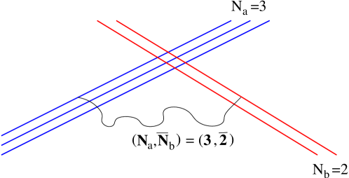
Figure 1: We find chiral matter at the intersection of two stacks of branes. The representation is given in terms of the number of branes of each stack.

In addition we get matter transforming in symmetric or antisymmetric representations of the gauge group for each individual stack. The multiplicities of these representations are given by the intersection numbers of the three-cycles,

$$I_{ab}:=\pi_{a}\circ\pi_{b}=\sum_{I=1}^{b_{3}/2}\left(X_{a}^{I}Y_{b}^{I}-X_{b}^{I}Y_{a}^{I}\right).$$ (3)

The possible representations are summarized in table 1, where $\mathbf{Sym}_{a}$ and $\mathbf{Anti}_{a}$ are the symmetric and antisymmetric representations of $U(N_{a})$.

representations	multiplicity
$(\mathbf{N}_{a},\overline{\mathbf{N}}_{b})$	$\pi_{a}\circ\pi_{b}=I_{ab}$
$(\mathbf{N}_{a},\mathbf{N}_{b})$	$\pi^{\prime}_{a}\circ\pi_{b}=I_{ab^{\prime}}$
$\mathbf{Sym}_{a}$	$\frac{1}{2}\left(\pi_{a}\circ\pi^{\prime}_{a}-\pi_{a}\circ\pi_{O6}\right)=\frac{1}{2}(I_{aa^{\prime}}-I_{a{\rm O}6})$
$\mathbf{Anti}_{a}$	$\frac{1}{2}\left(\pi_{a}\circ\pi^{\prime}_{a}+\pi_{a}\circ\pi_{O6}\right)=\frac{1}{2}(I_{aa^{\prime}}+I_{a{\rm O}6})$

Table 1: Multiplicities of the chiral spectrum.

2.1.2 Tadpole cancellation conditions

The D6-branes in our models are charged under a R-R seven-form [87]. Since the internal manifold is compact, as a simple consequence of the Gauss law, all R-R charges have to add up to zero. These so-called tadpole cancellation conditions can be obtained considering the part of the supergravity Lagrangian that contains the corresponding contributions. In particular we do not only get contributions from $k$ stacks of branes, wrapping cycles $\pi_{a}$, but in addition terms from the orientifold mirrors of these branes, wrapping cycles $\pi^{\prime}_{a}$, and the O6-planes.

$$S=-\frac{1}{4\kappa^{2}}\int\limits_{X\times M}dC_{7}\wedge\star dC_{7}+\mu_{6}\sum_{a=1}^{k}N_{a}\left(\int\limits_{X\times\pi_{a}}C_{7}+\int\limits_{X\times\pi^{\prime}_{a}}C_{7}\right)-4\mu_{6}\int\limits_{X\times\pi_{O6}}C_{7},$$ (4)

where the ten dimensional gravitational coupling is given by $\kappa^{2}=\frac{1}{2}(2\pi)^{7}(\alpha^{\prime})^{4}$, the R-R charge is denoted by $\mu_{6}=(\alpha^{\prime})^{-\frac{7}{2}}(2\pi)^{-6}$ and $X$ denotes the uncompactified space-time.

From this we can derive the equations of motion for the R-R field strength $G_{8}=dC_{7}$ to be

$$d\star G_{8}=\kappa^{2}\mu_{6}\left(\sum_{a=1}^{k}N_{a}\left(\delta(\pi_{a})+\delta(\pi^{\prime}_{a})\right)-4\delta(\pi_{O6})\right).$$ (5)

In this equation $\delta(\pi)$ denotes the Poincaré dual three form of a cycle $\pi$. Noticing that the left hand side of (5) is exact, we can rewrite this as a condition in homology as

$$\sum_{a=1}^{k}N_{a}(\pi_{a}+\pi^{\prime}_{a})=4\pi_{O6}$$ (6)

We do not have to worry about the NS-NS tadpoles, as long as we are considering supersymmetric models, since the supersymmetry conditions together with R-R tadpole cancellation ensure that there are no NS-NS tadpoles. In the following we consider supersymmetric models only.

2.1.3 Supersymmetry conditions

Since we want to analyse supersymmetric models, it is crucial that the D-branes and O-planes preserve half of the target-space supersymmetry. It can be shown [83] that this requirement is equivalent to a calibration condition on the cycles,

$$\Im(\Omega_{3})|_{\pi_{a}}=0,\qquad\Re(\Omega_{3})|_{\pi_{a}}>0,$$ (7)

where $\Omega_{3}$ is the holomorphic 3-form. The second equation in (7) excludes anti-branes from the spectrum.

Written in the symplectic basis (1), these equations read

$$\sum_{I=1}^{b_{3}/2}Y_{a}^{I}f_{I}=0,\qquad\sum_{I=1}^{b_{3}/2}X_{a}^{I}u_{I}>0,$$ (8)

where we defined

$$f_{I}:=\int_{\beta_{I}}\Omega_{3},\qquad u_{I}:=\int_{\alpha_{I}}\Omega_{3}.$$

2.1.4 Anomalies and K-theory constraints

If the tadpole cancellation conditions (6) are satisfied, there are no cubic anomalies of $SU(N)$ gauge groups in our models. What we do have to worry about are mixed anomalies, containing abelian factors. The mixed anomaly for branes stretching between two stacks $a$ and $b$ with $N_{a}=1$ and $N_{b}>1$ branes per stack, looks like

$$\mathcal{A}_{U(1)_{a}-SU(N)_{b}}\simeq N_{a}(I_{ab}+I_{ab^{\prime}})c_{2}(N_{b})=-2N_{a}\vec{Y_{a}}\vec{X_{b}}c_{2}(N_{b}),$$ (9)

where $c_{2}(N_{b})$ denotes the value of the quadratic Casimir operator for the fundamental representation of $SU(N_{b})$.

The cubic anomaly consisting of three abelian factors is cancelled by the Green-Schwarz mechanism. This makes these $U(1)$s massive and projects them out of the low energy spectrum. But in some cases, for example in the case of a standard model-like gauge group or for flipped $SU(5)$ models, we want to get a massless $U(1)$ factor. A sufficient condition to get such a massless $U(1)$ in one of our models is that the anomaly (9) vanishes.

This can be archived, if the $U(1)$, defined in general by a combination of several $U(1)$ factors as

$$U(1)=\sum_{a=1}^{k}x_{a}U(1)_{a},$$ (10)

fulfills the following relations,

$$\sum_{a=1}^{k}x_{a}N_{a}\vec{Y}_{a}=0.$$ (11)

Inserting this into (9) shows that $\mathcal{A}$ vanishes.

Besides these local gauge anomalies, there is also the potential danger of getting a global gauge anomaly, which would make the whole model inconsistent. This anomaly arises if a $\mathbb{Z}_{2}$-valued K-theory charge is not conserved [98]. In our case this anomaly can be derived by introducing $Sp(2)$ probe branes on top of the orientifold planes and compute their intersection numbers with all branes in the model. This intersection number has to be even, otherwise we would get an odd number of fermions, transforming in the fundamental representation of $Sp(2)$ [101].

2.2 Methods of D-brane statistics

To analyse a large class of models in the orientifold setting described in the last section, we have to develop some tools that allow us to generate as many solutions to the supersymmetry, tadpole and K-theory conditions as possible. It turns out that the most difficult part of this problem can be reduced to a purely number theoretical question, namely the problem of counting partitions of natural numbers. This insight allows us to use an approximative method, the saddle point approximation that we introduce in section 2.2.1 and apply to a simple toy-model in 2.2.2. Unfortunately it turns out that this method is not very well suited to study the most interesting compactifications, namely those down to four dimensions. Therefore we have to change the method of analysis in that case to a more direct one, using a brute force, exact computer analysis. The algorithm used to do so is described in section 2.2.3.

2.2.1 Introduction to the saddle point approximation

As an approximative method to analyse the gauge sector of type II orientifolds, the saddle point approximation has been introduced in [17]. In the following we begin with a very simple, eight-dimensional model, in order to explain the method.

In the most simple case, a compactification to eight dimensions on $T^{2}$, the susy conditions reduce to $Y_{a}=0$ and $X_{a}>0$ and the tadpole cancellation conditions are given by

$$\sum_{a=1}^{k}N_{a}\,X_{a}=16,$$ (12)

as shown in appendix A.1.

The task to count the number of solutions to this equation for an arbitrary number of stacks $k$ is a combination of a partitioning and factorisation problem. Let us take things slowly and start with a pure partitioning problem, namely to count the unordered solutions of

$$\sum_{a=1}^{k}N_{a}=L.$$ (13)

This is nothing else but the number of unordered partitions of $L$. Since we are not interested in an exact solution, but rather an approximative result, suitable for a statistical analysis and further generalisation to the more ambitious task of solving the tadpole equation, let us attack this by means of the saddle point approximation [2, 102].

As a first step to solve (13), let’s consider

$$\sum_{k=1}^{\infty}k\,n_{k}=L,$$ (14)

where we do not have to worry about the ordering problem. We can rewrite this as

$$\mathcal{N}(L)=\sum_{all}\delta_{\sum_{k}\,kn_{k}-L,0}=\frac{1}{2\pi i}\oint dq\frac{1}{q^{L+1}}\sum_{n_{k}=0}^{\infty}q^{\sum_{k}\,kn_{k}}=\frac{1}{2\pi i}\oint dq\frac{1}{q^{L+1}}\prod_{k=1}^{\infty}\left(\frac{1}{1-q^{k}}\right).$$ (15)

To evaluate integrals of this type in an asymptotic expansion, the saddle point method is a commonly used tool. In the following we describe its application in detail. The last line of (15) can be written as

$$\mathcal{N}(L)=\frac{1}{2\pi i}\oint{dq}\,\exp(f(q)),\quad\mbox{with}\quad f(q)=-\sum_{k=1}^{\infty}\log(1-q^{k})-(L+1)\,\log q.$$ (16)

Now we are going to assume that the main contributions to this integral come from saddle points $q_{i}$, determined by $\left.df/dq\right|_{q_{i}}=0$. In the following we work with only one saddle point at $q=q_{0}$, the generalisation to many points is always straightforward. Using the decomposition $q=\rho\exp(i\varphi)$ we get

$$\mathcal{N}(L)=\frac{1}{2\pi}\int\limits_{-\pi}^{\pi}d\varphi\,q\,\exp(f(q)).$$ (17)

Performing a Taylor expansion in $\varphi$

$$f(\rho_{0},\varphi)=f(q_{0})+\left.\frac{1}{2}\,\frac{\partial^{2}f}{\partial\varphi^{2}}\right|_{q_{0}}\,\varphi^{2}+\ldots,$$ (18)

we can compute (17) to arbitrary order by inserting the corresponding terms from (18).

The leading order term is simply given by

$$\mathcal{N}^{(0)}(L)=\exp(f(q_{0})),$$ (19)

and the first correction at next-to-leading order by

$$\mathcal{N}^{(2)}_{corr}(L)=\frac{1}{2\pi}\int\limits_{-q_{0}\pi}^{q_{0}\pi}dx\,\exp\left(-\frac{1}{2}\left.\frac{\partial^{2}f}{\partial q^{2}}\right|_{q_{0}}x^{2}\right),$$ (20)

where we defined $x:=q_{0}\varphi$ and used that $(\partial^{2}f/\partial\varphi^{2})_{q_{0}}=-q^{2}\,(\partial^{2}f/\partial q^{2})_{q_{0}}$. For $\partial^{2}f/\partial q^{2}$ large enough we finally obtain the result for the saddle point approximation including next-to-leading order corrections

$$\mathcal{N}^{(2)}(L)=\frac{1}{2\pi}\,\exp(f(q_{0}))\left(\left.\frac{\partial^{2}f}{\partial q^{2}}\right|_{q_{0}}\right)^{-1/2}.$$ (21)

The same procedure can also be performed for functions of several variables. The integral to approximate this situation looks like

$$\mathcal{N}(\vec{L})=\frac{1}{2\pi i}\oint\prod_{I=1}^{n}{d\vec{q}}\,\exp(f(\vec{q})),$$ (22)

with $f$ being of the form

$$f(\vec{q})=g(\vec{q})-\sum_{I=1}^{N}(L_{I}+1)\,\log q_{I}.$$ (23)

We can perform the saddle point approximation around $\nabla f(\vec{q})|_{\vec{q}_{0}}=0$ in the same way as above and obtain the following result at next-to-leading order

$$\mathcal{N}^{(2)}(\vec{L})=(2\pi)^{-n/2}\,\exp(f(\vec{q_{0}}))\left(\left.\det\mathrm{Hess}f(\vec{q})\right|_{\vec{q_{0}}}\right)^{-1/2}.$$ (24)

In the simple case discussed so far, contrary to the more complicated cases we encounter later, an analytic evaluation of the leading order contribution is possible. For large $L$ the integrand of (15) quickly approaches infinity for $q<1$ and $q\simeq 1$. One expects a sharp minimum close to 1, which would be the saddle point we are looking for.

Close to $q\simeq 1$ we can write the first term in (16) as

$$-\sum_{k=1}^{\infty}\log(1-q^{k})=\sum_{k,m>0}\frac{1}{m}q^{km}\simeq\frac{1}{1-q}\sum_{m>0}\frac{1}{m^{2}}=\frac{\pi^{2}}{6}\,\frac{1}{1-q},$$ (25)

such that we can approximate $f(q)$ by

$$f(q)\simeq\frac{\pi^{2}}{6}\,\frac{1}{1-q}-(L+1)\,\log q.$$ (26)

For large values of $L$, the minimum of this function is approximately at $q_{0}\simeq 1-\sqrt{\frac{\pi^{2}}{6L}}$ which leads to $f(q_{0})\simeq\pi\sqrt{2L/3}$. Inserting this into (19) gives a first estimate of the growth of the partitions for large $L$ to be

$$\mathcal{N}(L)\simeq\exp\left(\pi\sqrt{2L/3}\right).$$ (27)

This is precisely the leading term in the Hardy-Ramanujan formula [73] for the asymptotic growth of the number of partitions

$$\mathcal{N}(L)^{(HR)}\simeq\frac{1}{4L\sqrt{3}}\,\exp\left(\pi\sqrt{2L/3}\right).$$ (28)

Figure 2: Comparison of the number of partitions obtained by an exact calculation (solid line) and a saddle point approximation to leading (upper dotted line) and next-to-leading order (lower dotted line).

In figure 2 the results of an exact calculation, using the partition algorithm described in appendix B, and the saddle point approximation in leading and next-to-leading order are shown.

2.2.2 A first application of the saddle point approximation

After this introduction to the saddle point method let us come back to our original problem. To solve equation (12), we first have to transfer our approximation method to (13) and then include the factorisation in the computation. This last step turns out not to be too difficult, but in order to use the technique developed above, we have to be a bit careful about the ordering of solutions.

In the example we presented to introduce the method, we did not have to worry about the ordering, since it was solved implicitly by the definition of the partition function. This is not the case for (13), such that by simply copying from above the result is too large. We should divide the result by the product of the number of possibilities to order each partition. Obtaining this factor precisely is very difficult and since we are only interested in an approximative result anyway, we should try to estimate the term. Such an estimate can be made dividing by $k!$, where $k$ is the total number of stacks. This restricts the number of solutions more than necessary, because the factor is too high for partitions that contain the same element more than once. Let us nevertheless calculate the result with this rough estimate and see what comes out.

Repeating the steps from above, we can rewrite (13) to obtain

$$\widetilde{\mathcal{N}}(L) \simeq \frac{1}{2\pi i}\oint dq\frac{1}{q^{L+1}}\sum_{k=1}^{\infty}\frac{1}{k!}\,\prod_{i=1}^{k}\left(\sum_{N_{i}=1}^{\infty}q^{\sum_{a}\,N_{a}}\right)=\frac{1}{2\pi i}\oint dq\frac{1}{q^{L+1}}\sum_{k=1}^{\infty}\frac{1}{k!}\,\left(\sum_{N=1}^{\infty}q^{N}\right)^{k}$$ (29)

$$= \frac{1}{2\pi i}\oint dq\frac{1}{q^{L+1}}\sum_{k=1}^{\infty}\frac{1}{k!}\,\left(\frac{q}{1-q}\right)^{k}=\frac{1}{2\pi i}\oint dq\frac{1}{q^{L+1}}\exp\left(\frac{q}{1-q}\right).$$

Applying the saddle point approximation as explained above for the function

$$\tilde{f}(q)=\frac{q}{1-q}-(L+1)\log q,$$ (30)

we get for the number of solutions of (13) the estimate

$$\widetilde{\mathcal{N}}(L)\simeq\exp(2\sqrt{L}).$$ (31)

Comparing this result with  (27) shows that we get the correct exponential growth, but the coefficient is too small by a factor

$$\frac{\log\mathcal{N}}{\log\widetilde{\mathcal{N}}}=\frac{\pi}{\sqrt{6}}\simeq 1.28.$$ (32)

Figure 3: Comparing the results for the number of partitions of $L$. The solid line is the exact result, the dotted line is the saddle point approximation to leading order. The stars and triangles show the next-to-leading order result, without and including the additional analytic factor 1.28, respectively.

In figure 3 we compare the results for the leading and next-to-leading order results of the computation above with the exact result. As already expected, the value for the second order approximation is too small, since our suppression factor $k!$ is too big. Nevertheless, qualitatively the results are correct. Since we are not aiming at exact results, but rather at an approximative method to get an idea of the frequency distributions of properties of the models under consideration, this is not a big problem.

Let us finally come back to the full tadpole equation (12). It can be treated in the same way as the pure partition problem and analogous to (29) we can write

$$\mathcal{N}(L) \simeq \frac{1}{2\pi i}\oint dq\frac{1}{q^{L+1}}\sum_{k=1}^{\infty}\frac{1}{k!}\,\prod_{i=1}^{k}\left(\sum_{N_{i}=1}^{\infty}\sum_{X_{i}=1}^{L}q^{\sum_{a}\,N_{a}X_{a}}\right)$$ (33)

$$= \frac{1}{2\pi i}\oint dq\frac{1}{q^{L+1}}\sum_{k=1}^{\infty}\frac{1}{k!}\,\left(\sum_{X=1}^{L}\frac{q^{X}}{1-q^{X}}\right)^{k},$$

such that we obtain for $f$

$$f(q)=\sum_{X=1}^{L}\frac{q^{X}}{1-q^{X}}-(L+1)\log q.$$ (34)

Close to $q\simeq 1$ we can approximate this to

$$f(q)\,\simeq\,\frac{1}{1-q}\sum_{X=1}^{L}\frac{1}{X}-L\log q\,\simeq\,\frac{\log L}{1-q}-L\log q.$$ (35)

The minimum can then be found at $q_{0}\simeq 1-\sqrt{\frac{\log L}{L}}$, which gives for the number of solutions

$$\mathcal{N}(L)\simeq\exp(2\sqrt{L\log L}).$$ (36)

The additional factor of $\log L$ in the scaling behaviour compared to (31) can be explained by a result from number theory. It is known that the function $\sigma_{0}(n)$, counting number of divisors of an integer $n$, has the property

$$\frac{1}{L}\sum_{n=1}^{L}\sigma_{0}(n)\simeq\log L+(2\gamma_{E}-1),$$ (37)

where $\gamma_{E}$ is the Euler-Mascheroni constant.

Figure 4: Logarithmic plot of the number of solutions to the supersymmetry and tadpole equations for compactifications on $T^{2}$. The dotted line shows the exact results, the solid line is the result of a next-to-leading order saddle point approximation.

Let us compare the result (36) with the exact number of solutions, obtained with a brute force computer analysis. This is shown in figure 4. As expected from the discussion above, the estimate using the saddle point approximation is too small, but it has the correct scaling behaviour and should therefore be suitable to qualitatively analyse the properties of the solutions.

We can use the saddle point approximation method introduced above to analyse several properties of the gauge sector of the models. To show how this works, we present two examples in the simple eight-dimensional case, before applying these methods in section 3.1 to models on $T^{4}/\mathbb{Z}_{2}$.

One interesting observable is the probability to find an $SU(M)$ gauge factor in the total set of models. Using the same reasoning as in the computation of the number of models this is given by

$$P(M,L) \simeq \frac{1}{2\pi i\mathcal{N}(L)}\oint dq\frac{1}{q^{L+1}}\sum_{k=1}^{\infty}\frac{1}{(k-1)!}\left(\sum_{X=1}^{L}\frac{q^{X}}{1-q^{X}}\right)^{k-1}\sum_{X=1}^{L}\sum_{N=1}^{\infty}q^{NX}\delta_{N,M}$$ (38)

$$= \frac{1}{2\pi i\mathcal{N}(L)}\oint dq\frac{1}{q^{L+1}}\exp\left(\sum_{X=1}^{L}\frac{q^{X}}{1-q^{X}}\right)q^{M}\frac{1-q^{ML}}{1-q^{M}}.$$

The saddle point function is therefore given by

$$f(q)=\sum_{X=1}^{L}\frac{q^{X}}{1-q^{X}}+\log\left(q^{M}\frac{1-q^{ML}}{1-q^{M}}\right)-(L+1)\log q.$$ (39)

A comparison between exact computer results and the saddle point approximation to second order is shown in figure 5(a).

(a)

(b)

Figure 5: Distributions for compactifications on $T^{2}$. The solid lines are the exact result, the dotted lines represent the second order saddle point approximation. (a) Probability to find at least one $SU(M)$ gauge factor. (b) Frequency distribution of the total rank.

Another observable we are interested in is the distribution of the total rank of the gauge group in our models. This amounts to including a constraint

$$\sum_{a=1}^{\infty}N_{a}=r,$$ (40)

that fixes the total rank to a specific value $r$. This constraint can be accounted for by adding an additional delta-function, represented by an additional contour integral to our formula. We obtain

$$P(r,L) \simeq \frac{1}{2\pi i\mathcal{N}(L)}\oint dq\frac{1}{q^{L+1}}\oint dz\frac{1}{z^{r+1}}\sum_{k=1}^{\infty}\frac{1}{k!}\prod_{i=1}^{k}\left(\sum_{N_{i}=1}^{\infty}\sum_{X_{i}=1}^{L}q^{\sum_{a}N_{a}X_{a}}z^{\sum_{a}N_{a}}\right)$$ (41)

$$= \frac{1}{2\pi i\mathcal{N}(L)}\oint dq\frac{1}{q^{L+1}}\oint dz\frac{1}{z^{r+1}}\exp\left(\sum_{X=1}^{L}\frac{zq^{X}}{1-zq^{X}}\right),$$

with saddle point function

$$f(q,z)=\sum_{X=1}^{L}\frac{zq^{X}}{1-zq^{X}}-(L+1)\log q-(r+1)\log z.$$ (42)

As we can see in figure 5(b), where we also show the exact computer result, we get a Gaussian distribution.

2.2.3 Exact computations

Instead of using an approximative method, it is also possible to directly calculate possible solutions to the constraining equations. At least for models on $T^{2}$ or $T^{4}/\mathbb{Z}_{2}$, this is much more time-consuming than the saddle point approximation, and, what is even more important, cannot be done completely for models on $T^{6}/\mathbb{Z}_{2}\!\times\!\mathbb{Z}_{2}$. The reason why a complete classification is not possible has to do with the fact that the problem to find solutions to the supersymmetry and tadpole equations belongs to the class of NP-complete problems, an issue that we elaborate on in section 2.3. Despite these difficulties, it turns out to be necessary to use an explicit calculation for four-dimensional compactifications, the ones we are most interested in, since the saddle point method does not lead to reliable results in that case.

In the eight-dimensional case the algorithmic solution to the tadpole equation

$$\sum_{a}N_{a}\,X_{a}=L,$$ (43)

can be formulated as a two-step algorithm. First calculate all possible unordered partitions of $L$, then find all possible factorisations to obtain solutions for $X$ and $N$. The task of partitioning is solved by the algorithm explained in appendix B, the factorisation can only be handled by brute force. In this way we are not able to calculate solutions up to very high values for $L$, but for our purposes, namely to check the validity of the saddle point approximation (see section 2.2.2), the method is sufficient.

In the case of compactifications to six dimensions we can still use the same method, although we now have to take care of two additional constraints. First of all we exclude multiple wrapping, which gives an additional constraint on the wrapping numbers $X_{1},X_{2},Y_{1}$ and $Y_{2}$, defined in appendix A.3. This constraint can be formulated in terms of the greatest common divisors of the wrapping numbers – we will come back to this issue in section 3.1. Another difference compared to the eight dimensional case is that we have to take different values for the complex structure parameters $U_{1}$ and $U_{2}$ (see appendix A.3 for a definition) into account. As it is shown in section 2.3, these are bounded from above and we have to sum over all possible values, making sure that we are not double counting solutions with wrapping numbers which allow for different values of the complex structures.

In (A.3) the wrapping numbers $\vec{X}$ and $\vec{Y}$ are defined as integer valued quantities in order to implement the supersymmetry (103) and tadpole (102) conditions in a fast computer algorithm. From the equations we can derive the following inequalities

$$0<\sum_{I=0}^{3}X^{I}\,{U}_{I}\leq\sum_{I=0}^{3}L^{I}\,{U}_{I}.$$ (44)

The algorithm to find solutions to these equations and the additional K-theory constraints (105) consists of four steps.

1. First we choose a set of complex structure variables $U_{I}$. This is done systematically and leads to a loop over all possible values. Furthermore, we have to check for redundancies, which might exist because of trivial symmetries under the exchange of two of the three two-tori.

2. In a second step we determine all possible values for the wrapping numbers $X^{I}$ and $Y^{I}$, using (44) for the given set of complex structures, thereby obtaining all possible supersymmetric branes. In this step we also take care of the multiple wrapping constraint, which can be formulated, analogously to the six dimensional case, in terms of the greatest common divisors of the wrapping numbers.

3. In the third and most time-consuming part, we use the tadpole equations (102), which after a summation can be written as

   $$\sum_{a=0}^{k}S_{a}=\Lambda\quad\mbox{with}\quad S_{a}:=\sum_{I=0}^{3}N_{a}{U}_{I}X_{a}^{I}\quad\mbox{and}\quad\Lambda:=\sum_{I}L^{I}{U}_{I}.$$ (45)

   To solve this equation, we note that all $S_{a}$ and $\Lambda$ are positive definite integers, which allows us to use the partition algorithm to obtain all possible combinations. The algorithm is improved by using only those values for the elements of the partition which are in the list of values we computed in the second step. For a detailed description of the explicit algorithm we used, see appendix B. Having obtained the possible $S_{a}$, we have to factorise them into values for $N_{a}$ and $X_{a}^{I}$.

4. Since (45) is only a necessary but no sufficient condition, we have to check in the fourth and last step, if the obtained results indeed satisfy all constraints, especially the individual tadpole cancellation conditions and the restrictions from K-theory, which up to this point have not been accounted for at all.

The described algorithm has been implemented in C and was put on several high-performance computer clusters, using a total CPU-time of about $4\times 10^{5}$ hours. The solutions obtained in this way have been saved in a database for later analysis.

The main problem of the algorithm described in the last section lies in the fact that its complexity scales exponentially with the complex structure parameters. Therefore we are not able to compute up to arbitrarily high values for the $U_{I}$. Although we tried our best, it may of course be possible to improve the algorithm in many ways, but unfortunately the exponential behaviour cannot be cured unless we might have access to a quantum computer. This is due to the fact that the number of possib le solutions to the Diophantine equations we are considering grows exponentially with $U$. In fact, this is quite a severe issue since the Diophantine structure of the tadpole equations encountered here is not at all exceptional, but very generic for the topological constraints also in other types of string constructions. The problem seems indeed to appear generically in computations of landscape statistics, see [41] for a general account on this issue.

As we outlined in the previous section, the computational effort to generate the solutions to be analysed in the next section took a significant amount of time, although we used several high-end computer clusters. To estimate how many models could be computed in principle, using a computer grid equipped with contemporary technology in a reasonable amount of time, the exponential behaviour of the problem has to be taken into account. Let us be optimistic and imagine that we would have a total number of $10^{5}$ processors at our disposal which are twice as fast as the ones we have been using. Expanding our analysis to cover a range of complex structures which is twice as large as the one we considered would, in a very rough estimate, still take us of the order of 500 years.

Note that in principle there can be a big difference in the estimated computing time for the two computational problems of finding all string vacua in a certain class on the one hand, and of looking for configurations with special properties, that lead to additional constraints, on the other hand. As we explore in section 3.5.3 the computing time can be significantly reduced if we restrict ourselves to a maximum number of stacks in the hidden sector and take only configurations of a specific visible sector into account (in the example we consider we look for grand unified models with an $SU(5)$ gauge group). Nevertheless, although a much larger range of complex structures can be covered, the scaling of the algorithm remains unchanged. This means in particular that a cutoff on the $U_{I}$, even though it might be at higher values, has to be imposed.

2.3 Finiteness of solutions

It is an important question whether or not the number of solutions is infinite. Making statistical statements about an infinite set of models is much more difficult than to deal with a finite sample, because we would have to rely on properties that reoccur at certain intervals, in order to be able to make any valuable statements at all. If instead the number of solutions is finite, and we can be sure that the solutions we found form a representative sample, it is possible to draw conclusions by analysing the frequency distributions of properties without worrying about their pattern of occurrence within the space of solutions.

In the case of compactifications to eight dimensions, the results are clearly finite, as can be seen directly from the fact that the variables $X$ and $N$ have to be positive and $L$ has a fixed value. Note however, although such an eight-dimensional model is clearly not realistic, that the complex structures are unconstrained. This means that if we do not invoke additional methods to fix their values, each solution to the tadpole equation represents in fact an infinite family of solutions.

2.3.1 The six-dimensional case

In the six dimensional case, the finiteness of the number of solutions is not so obvious, but it can be rigorously proven. In order to do so, we have to show that possible values for the complex structure parameters $U_{1}$ and $U_{2}$ are bounded from above. If this were not be the case, we could immediately deduce from equations (103) that infinitely many brane configurations would be possible.

In contrast to the eight-dimensional toy-model that we explored in section 2.2.2, in this case, and also for the four-dimensional compactifications, we do not want to allow branes that wrap the torus several times. To exclude this, we can derive the following condition on the wrapping numbers (for details see appendix A.2.1),

$$\gcd(X^{1},Y^{2})\gcd(X^{2},Y^{2})=Y^{2}.$$ (46)

This condition implies that all $\vec{X}$ and $\vec{Y}$ are non-vanishing. Additional branes, which wrap the same cycles as the orientifold planes, are given by $\vec{X}\in\left\{(1,0),(0,1)\right\}$, with $\vec{Y}=\vec{0}$ in both cases.

From (103) we conclude that all non-trivial solutions have to obey $U_{1}/U_{2}\in\mathbb{Q}$. Therefore we can restrict ourselves to coprime values

$$(u_{1},u_{2})\quad\mbox{with}\quad u_{i}:=\frac{U_{i}}{\gcd(U_{1},U_{2})}.$$ (47)

With these variables we find from the supersymmetry conditions that $Y^{1}=u_{2}\,\alpha$, for some $\alpha\in\mathbb{Z}$. Now we can use the relation (90) to get

$$X^{1}\,X^{2}=u_{1}\,u_{2}\,\alpha^{2}.$$ (48)

In total we get two classes of possible branes, those where $X^{1}$ and $X^{2}$ are both positive and those where one of them is $0$. The latter are those where the branes lie on top of the orientifold planes.

For fixed values of $u_{1}$ and $u_{2}$ the tadpole cancellation conditions (92) admit only a finite set of solutions. Since all quantities in these equations are positive, we can furthermore deduce from (48) that solutions which contain at least one brane with $X^{1},X^{2}>0$ are only possible if the complex structures satisfy the bound

$$u_{1}u_{2}\leq L_{1}L_{2}.$$ (49)

In figure 6 we show the allowed values for $u_{1}$ and $u_{2}$ that satisfy equation (49).

Figure 6: Allowed values for the complex structure parameters $u_{1}$ and $u_{2}$ for compactifications to six dimensions.

In the case that only branes with one of the $X^{i}$ vanishing are present in our model, the complex structures are not bounded from above, but since there exist only two such branes in the case of coprime wrapping numbers, all solutions of this type are already contained in the set of solutions which satisfy (49). Therefore we can conclude that the overall number of solutions to the constraining equations in the case of compactifications to six dimensions is finite.

2.3.2 Compactifications to four dimensions

The four dimensional case is very similar to the six-dimensional one discussed above, but some new phenomena appear. In particular, we see that the wrapping numbers can have negative values, which is the crucial point that prevents us from proving the finiteness of solutions. Although we were not able to obtain an analytic proof, we present some arguments and numerical results, which provide evidence and make it very plausible that the number of solutions is indeed finite.

As in the $T^{4}/\mathbb{Z}_{2}$ case, we can derive a condition on the (rescaled) wrapping numbers $\vec{X}$ and $\vec{Y}$, defined by (A.3.1), to exclude multiple wrapping. The derivation is given in appendix A.3.1 and the result is

$$\prod_{i=1}^{3}\gcd(\tilde{Y}^{0},\tilde{X}^{i})=(\tilde{Y}^{0})^{2}.$$ (50)

From the relations (100), it follows that either one, two or all four $X^{I}$ can be non-vanishing. The case with only one of them vanishing is excluded. Let us consider the three possibilities in turn and see what we can say about the number of possible solutions in each case.

1. In the case that only one of the $X^{I}\neq 0$, the corresponding brane lies on top of one of the orientifold planes on all three $T^{2}$. This situation is equivalent to the eight-dimensional case and can be included in the discussion of the next possibility.

2. If two $X^{I}\neq 0$, we are in the situation discussed for the compactification to six dimensions. The two $X^{I}$ have to be positive by means of the supersymmetry condition and one of the complex structures is fixed at a rational number. Together with the eight-dimensional branes, the same proof of finiteness we have given for the $T^{4}/\mathbb{Z}_{2}$-case can be applied.

3. A new situation arises for those branes where all $X^{I}\neq 0$. Let us discuss this a bit more in detail.

From the relations (100) we deduce that an odd number of them has to be negative. In the case that three would be negative and one positive – let us without loss of generality choose $X_{0}>0$ – we can write the supersymmetry condition (103) as

$$\sum_{I=0}^{3}Y^{I}\frac{1}{U_{I}}=\frac{Y^{0}}{U_{0}}\left(1+\sum_{i=1}^{3}\frac{X^{0}\,U_{0}}{X^{i}\,U_{i}}\right)=0,$$ (51)

which implies $X^{i}\,U_{i}<-X^{0}\,U_{0}\,\,\forall\,i\in\{1,2,3\}$. This contradicts the second supersymmetry condition,

$$X^{0}\,U_{0}\left(1+\sum_{i=1}^{3}\frac{X^{i}\,U_{i}}{X^{0}\,U_{0}}\right)>0.$$ (52)

Therefore, we conclude that the only remaining possibility is to have one of the $X^{I}<0$. Again we choose $X^{0}$ without loss of generality. We can now use (51) to express $X^{0}$ in terms of the other three wrapping numbers as

$$X^{0}=-\left(\sum_{i}\frac{U_{0}}{U_{i}\,X^{i}}\right)^{-1}.$$ (53)

Furthermore, we can use the inequality (44) and derive an upper bound

$$\sum_{I=0}^{3}L_{I}\,U_{I}\,\geq\,X^{0}\ U_{0}+\sum_{i=1}^{3}X^{i}\,U_{i}\,>\,X^{j}\,U_{j}\,>\,0,\quad\forall\,j\in\{1,2,3\}.$$ (54)

As in the six-dimensional case, we can use the argument that the complex structures are fixed at rational values, as long as we take a sufficient number of branes. So we can write them, in analogy to (47) as $u_{I,2}/u_{I,1}$. Using this definition, we can write (54) as

$$1\leq X_{i}\leq\frac{\sum_{P=0}^{3}u_{P,2}u_{Q,1}u_{R,1}u_{S,1}L_{P}}{u_{i,2}u_{J,1}u_{K,1}u_{L,1}},$$ (55)

for $P\neq Q\neq R\neq S\neq P$ and $i\neq J\neq K\neq L\neq i$.

From this we conclude that as long as the complex structures are fixed, we have only a finite number of possible brane configurations, i.e. only a finite number of solutions. This is unfortunately not enough to conclude that we have only a finite number of solutions in general. We would have to show, as in the six-dimensional case, that there exists an upper bound on the complex structures. Since we were not able to find an analytic proof that such a bound exists, we have to rely on some numerical hints that it is in fact the case. We present some of these hints in the following.

Figure 7: The number of unique solutions for compactifications on $T^{6}/\mathbb{Z}_{2}\!\times\!\mathbb{Z}_{2}$, taking $L_{I}=2$ $\forall I\in\{0,\ldots,3\}$. The horizontal axis shows combinations of the $U_{I}$, ordered by their absolute value $|U|$. For each of these values we plotted the cumulative set of solutions obtained up to this point.

Figure 7 shows how the total number of mutually different brane configurations for $L=2$ increases and saturates, as we include more and more combinations of values for the complex structures $U_{I}$ into the set for which we construct solutions. For this small value of $L$ our algorithm actually admits pushing the computations up to those complex structures where obviously no additional brane solutions exist.

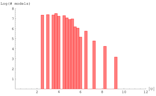
Figure 8: Logarithmic plot of the absolute number of solutions for compactifications on $T^{6}/\mathbb{Z}_{2}\!\times\!\mathbb{Z}_{2}$ using the physical values $L_{I}=8$ $\forall I\in\{0,\ldots,3\}$ against the absolute value $|U|$. The cutoff is set at $|U|=12$. In this plot, as in all other plots of this paper, we use a decadic logarithm.

For the physically relevant case of $L=8$ the total number of models compared to the absolute value $|U|$ of the complex structure variables scales as displayed in figure 8. The plot shows all complex structures we have actually been able to analyse systematically. We find that the number of solutions falls logarithmically for increasing values of $|U|$. In order to interpret this result, we observe that the complex structure moduli $U_{I}$ are only defined up to an overall rescaling by the volume modulus of the compact space. We have chosen all radii and thereby also all $U_{I}$ to be integer valued, which means that large $|U|$ correspond to large coprime values of $R_{1}^{(i)}$ and $R_{2}^{(i)}$. This comprises on the one hand decompactification limits which have to be discarded in any case for phenomenological reasons, but on the other hand also tori which are slightly distorted, e.g. almost square tori with $R_{2}^{(i)}/R_{1}^{(i)}=0.99$.

3 Statistical analysis of orientifold models

After preparing the stage in the last section, introducing the models and methods of analysis, we are now going to analyse some specific constructions of phenomenological interest. At the end of this section we want to arrive at a point where we can make some meaningful statistical statements about the probability to find realisations of the standard model or GUT models in the specific set of models we are considering.

However, it is important to mention, that our results cannot be regarded to be complete. First of all we neglect the impact of fluxes, which does not change the distributions completely, but definitely has some influence. Secondly, we are considering only very specific geometries. Since the construction of the orientifolds, especially the choice of the orbifold group which in our case is always $\mathbb{Z}_{2}$, has a strong impact on the constraining equations, it is very probable that the results change significantly once we use a different compactification space. Nevertheless we think that these results are one step towards a deeper understanding of open string statistics.

In the first part of this section we discuss some general aspects of compactifications to six and four dimensions. We analyse the properties of the gauge groups, including the occurrence of specific individual gauge factors and the total rank. With respect to the chiral matter content, we establish the notion of a mean chirality and discuss their frequency distribution.

In a second part we perform a search for models with the properties of a supersymmetric standard model. Besides the frequency distributions in the gauge sector we analyse the values of the gauge couplings and compare our results to those of a recent statistical analysis of Gepner models [48, 49]. In addition to standard model gauge groups we look also for models with a Pati-Salam, $SU(5)$ and flipped $SU(5)$ structure.

In the last part we consider different aspects of the question of correlations of observables in the gauge sector and give an estimate how likely it is to find a three generation standard model in our setup.

3.1 Statistics of six-dimensional models

Before considering the statistics of realistic four-dimensional models, let us start with a simpler construction to test the methods of analysis developed in section 2. We will use a compactification to six dimensions on a $T^{4}/\mathbb{Z}_{2}$ orientifold, defined in appendix A.2. The important question about the finiteness of solutions has been settled in section 2.3, so we can be confident that the results we obtain will be meaningful. To use the saddle point approximation in this context, we have to generalise from the eight-dimensional example in 2.2.2 to an approximation in several variables, as described by equations (22) and (23). In our case we will have to deal with two variables $\vec{q}=(q_{1},q_{2})$, corresponding to the two wrapping numbers $\vec{X}=(X^{1},X^{2})$.

Figure 9: Logarithmic plot of the number of solutions for compactifications on $T^{4}/\mathbb{Z}_{2}$ for $L^{2}=8$ and different values of $L\equiv L^{1}$. The complex structures are fixed to $u_{1}=u_{2}=1$. The dotted line shows the result with multiple wrapping, the stared line gives the result with coprime wrapping numbers.

Let us briefly consider the question of multiple wrapping. As shown in appendix A.2.1, we can derive a constraint on the wrapping numbers $\vec{X}$ and $\vec{Y}$, such that multiply wrapping branes are excluded. To figure out what impact this additional constraint has on the distributions, let us compare the number of solutions for different values of $L^{1}$ and $L^{2}$, with and without multiple wrapping. The result is shown in figure 9. As could have been expected, the number of solutions with coprime wrapping numbers grows less fast then the one where multiple wrapping is allowed.

3.1.1 Distributions of gauge group observables

Using the saddle point method, introduced in section 2.2.1, we can evaluate the distributions for individual gauge group factors and total rank of the gauge group in analogy to the simple eight-dimensional example we pursued in section 2.2.2. Therefore we will fix the orientifold charges to their physical values, $\vec{L}=(L_{1},L_{2})=(8,8)$. The probability to find one $U(M)$ gauge factor can be written similar to (38) as

$$P(M,\vec{L}) \simeq \frac{1}{\mathcal{N}(\vec{L})(2\pi i)^{2}}\oint d\vec{q}\,\exp\Biggl{[}\sum_{\vec{X}\in S_{U}}\frac{q_{1}^{X_{1}}\,q_{2}^{X_{2}}}{1-q_{1}^{X_{1}}\,q_{2}^{X_{2}}}+\log\left(\sum_{\vec{X}\in S_{U}}q_{1}^{MX_{1}}q_{2}^{MX_{2}}\right)$$ (56)

$$-(L_{1}\!+\!1)\log q_{1}-(L_{2}\!+\!1)\log q_{2}\Biggl{]},$$

where we denoted with $S_{U}$ the set of all values for $\vec{X}$ that are compatible with the supersymmetry conditions and the constraints on multiple wrapping. The number of solution $\mathcal{N}(\vec{L})$ is given by

$$\mathcal{N}(\vec{L})\simeq\frac{q}{(2\pi i)^{2}}\oint d\vec{q}\,\exp\Biggl{[}\sum_{\vec{X}\in S_{U}}\frac{q_{1}^{X_{1}}\,q_{2}^{X_{2}}}{1-q_{1}^{X_{1}}\,q_{2}^{X_{2}}}-(L_{1}\!+\!1)\log q_{1}-(L_{2}\!+\!1)\log q_{2}\Biggl{]}.$$ (57)

The resulting distribution for the probability of an $U(M)$ factor, compared to the results of an exact computer search, is shown in figure 10(a).

(a)

(b)

Figure 10: Distributions in the gauge sector of a compactification on $T^{4}/\mathbb{Z}_{2}$. The complex structures are fixed to $u_{1}=u_{2}=1$. The dotted line is the result of an exact computation, the solid line shows the saddle point approximation to second order. (a) Probability to find an $(U(M)$ gauge factor, (b) Distribution of the total rank of the gauge group.

As in the eight-dimensional example we can evaluate the distribution of the total rank (40). As a generalisation of (41) we obtain the following formula

$$P(r,\vec{L}) \simeq \frac{1}{\mathcal{N}(\vec{L})(2\pi i)^{3}}\oint d\vec{q}dz\,\exp\Biggl{[}\sum_{\vec{X}\in S_{U}}\frac{zq_{1}^{X_{1}}q_{2}^{X_{2}}}{1-zq_{1}^{X_{1}}q_{2}^{X_{2}}}$$ (58)

$$-(L_{1}\!+\!1)\log q_{1}-(L_{2}\!+\!1)\log q_{2}-(r\!+\!1)\log z\Biggl{]}.$$

Figure 10(b) shows the resulting distribution of the total rank, compared to the exact result. As one can see, the results of the saddle point analysis are much smoother then the exact results, which show a more jumping behaviour, resulting from number theoretical effects. These are strong at low $L$, which is also the reason that our saddle point approximation is not very accurate. In the present six-dimensional case the deviations are not too strong, but in the four-dimensional case their impact is so big that the result cannot be trusted anymore. These problems can be traced back to the small values of $L$ we are working with, but since these are the physical values for the orientifold charge, we cannot do much about it.

3.1.2 Chirality

Since we are ultimately interested in calculating distributions for models with gauge groups and matter content close to the standard model, it would be interesting to have a measure for the mean chirality of the matter content in our models.

A good quantity to consider for this purpose would be the distribution of intersection numbers $I_{ab}$ between different stacks of branes. This is precisely the quantity we choose later in the four-dimensional compactifications. In the present case we use a simpler definition for chirality, given by

$$\chi:=X^{1}X^{2}.$$ (59)

This quantity counts the net number of chiral fermions in the antisymmetric and symmetric representations.

Using the saddle point method, we can compute the distribution of values for $\chi$, using

$$P(\chi,\vec{L}) \simeq \frac{1}{\mathcal{N}(\vec{L})(2\pi i)^{2}}\oint d\vec{q}\,\exp\Biggl{[}\sum_{\vec{X}\in S_{U}}\frac{q_{1}^{X_{1}}q_{2}^{X_{2}}}{1-q_{1}^{X_{1}}q_{2}^{X_{2}}}-\log\left(\sum_{\vec{X}\in S_{U}}\frac{q_{1}^{X_{1}}q_{2}^{X_{2}}}{1-q_{1}^{X_{1}}q_{2}^{X_{2}}}\right)$$ (60)

$$+\log\left(\sum_{\vec{X}\in S_{U,\chi}}\frac{q_{1}^{X_{1}}q_{2}^{X_{2}}}{1-q_{1}^{X_{1}}q_{2}^{X_{2}}}\right)-(L_{1}\!+\!1)\log q_{1}-(L_{2}\!+\!1)\log q_{2}\Biggl{]},$$

where $S_{U,\chi}\subset S_{U}$ is the set of wrapping numbers that fulfills (59).

Figure 11: Distribution of the mean chirality for $T^{4}/\mathbb{Z}_{2}$, $L^{1}=L^{2}=8$, $u_{1}=u_{2}=1$.

The resulting distribution is shown in figure 11. For the used values of $u_{1},u_{2}=1$, $\chi$ has to be a square, which can be directly deduced from the supersymmetry conditions (93). The scaling turns out to be roughly $P(\chi)\simeq\exp(-c\sqrt{\chi})$. From this result we can conclude that non-chiral models are exponentially more frequent than chiral ones. This turns out to be a general property of the orientifold models that also holds in the four-dimensional case.

3.1.3 Correlations

In this section we would like to address the question of correlations between observables for the first time. We come back to this issue in section 3.6. The existence of such correlations can be seen in figure 12, where we plotted the distributions of models with specific total rank and chirality. The connection between both variables is given by the tadpole cancellation conditions, which involve the $N_{a}$ used for the definition of the total rank in (40) and the wrapping numbers $\vec{X}_{a}$, which appear in the definition of the mean chirality $\chi$ in (59). The distribution can be obtained from

$$P(\chi,r,\vec{L}) \simeq \frac{1}{\mathcal{N}(\vec{L})(2\pi i)^{3}}\oint d\vec{q}dz\,\exp\Biggl{[}\sum_{\vec{X}\in S_{U}}\frac{zq_{1}^{X_{1}}q_{2}^{X_{2}}}{1-zq_{1}^{X_{1}}q_{2}^{X_{2}}}-\log\left(\sum_{\vec{X}\in S_{U}}\frac{zq_{1}^{X_{1}}q_{2}^{X_{2}}}{1-zq_{1}^{X_{1}}q_{2}^{X_{2}}}\right)$$ (61)

$$+\log\left(\sum_{\vec{X}\in S_{U,\chi}}\frac{zq_{1}^{X_{1}}q_{2}^{X_{2}}}{1-zq_{1}^{X_{1}}q_{2}^{X_{2}}}\right)-(L_{1}\!+\!1)\log q_{1}-(L_{2}\!+\!1)\log q_{2}$$

$$-(r\!+\!1)\log z\Biggl{]},$$

which is a straightforward combination of (58) and (60).

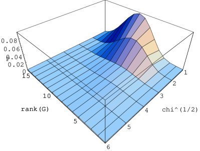
(a)

(b)

Figure 12: Correlation between total rank and chirality for $L_{1}=L_{2}=8$ and $u_{1}=u_{2}=1$ for a compactification on $T^{4}/\mathbb{Z}_{2}$. (b) shows the maximum of the total rank distribution depending on $\chi$.

In figure 12(a) one can see that the maximum of the rank distribution is shifted to smaller values for larger values of $\chi$. This could have been expected, since larger values of $\chi$ imply larger values for the wrapping numbers $\vec{X}$, which in turn require lower values for the number of branes per stack $N_{a}$, in order to fulfill the tadpole conditions. The shift of the maximum depending of $\chi$, can be seen more directly in figure 12(b).

3.2 Statistics of four-dimensional models

Having tried our methods in compactifications down to six dimensions, let us now switch to the phenomenologically more interesting case of four-dimensional models. Unfortunately we can no longer use the saddle point approximation, since it turns out that in this more complicated case the approximation is no longer reliable. The results deviate significantly from what we see in exact computations. Furthermore the computer power needed to obtain the integrals numerically in the approximation becomes comparable to the effort needed to compute the solutions explicitly.

3.2.1 Properties of the gauge sector

Using several computer clusters and the specifically adapted algorithm described in section 2.2.3 for a period of several months, we produced explicit constructions of $\approx~{}1.6\times 10^{8}$ consistent compactifications on $T^{6}/\mathbb{Z}_{2}\!\times\!\mathbb{Z}_{2}$. The results presented in the following have been published in [69, 68], see also the analysis in [78] and more recent results using brane recombination methods in [79].

Using this data we can proceed to analyse the observables of these models. The distribution of the total rank $r$ of the gauge group is shown in figure 13(a). An interesting phenomenon is the suppression of odd values for the total rank. This can be explained by the K-theory constraints and the observation that the generic value for $Y^{I}$ is 0 or 1. Branes with these values belong to the first class of branes in the classification of section 2.3.2 and are those which lie on top of the orientifold planes. Therefore equation (105) suppresses solutions with an odd value for $r$. This suppression from the K-theory constraints is quite strong, the total number of solutions is reduced by a factor of six compared to the situation where these constraints are not enforced.

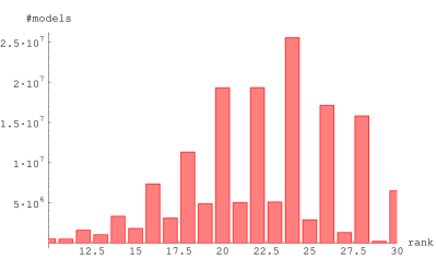
(a)

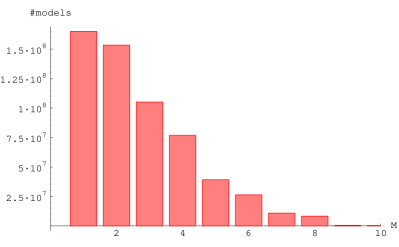
(b)

Figure 13: Frequency distributions of total rank and $U(M)$ gauge groups of all models.

Another quantity of interest is the distribution of $U(M)$ gauge groups, shown in figure 13(b). We find that most models carry at least one $U(1)$ gauge group, corresponding to a single brane, and stacks with a higher number of branes become more and more unlikely. This could have been expected because small numbers occur with a much higher frequency in the partition and factorisation of natural numbers.

3.2.2 Chirality

As in the six-dimensional case we want to define a quantity that counts chiral matter in the models under consideration. In contrast to the very rough estimate we used in section 3.1.2, this time we are going to count all chiral matter states, such that our definition of mean chirality is now

$$\chi:=\frac{2}{k(k+1)}\sum_{a,b=0,a<b}^{k}I_{a^{\prime}b}-I_{ab}=\frac{4}{k(k+1)}\sum_{a,b=0,a<b}^{k}\vec{Y}_{a}\vec{X}_{b}.$$ (62)

In this formula the states from the intersection of two branes $a$ and $b$ are counted with a positive sign, while the states from the intersection of the orientifold image of brane $a$, denoted by $a^{\prime}$, and brane $b$ are counted negatively. As we explained in section 2.1.1 and summarised in table 1, $I_{ab}$ gives the number of bifundamental representations $(\mathbf{N}_{a},\overline{\mathbf{N}}_{b})$, while $I_{a^{\prime}b}$ counts $(\overline{\mathbf{N}_{a}},\overline{\mathbf{N}_{b}})$. Therefore we compute the net number of chiral representations with this definition of $\chi$. By summing over all possible intersections and normalising the result we obtain a quantity that is independent of the number of stacks and can be used for a statistical analysis.

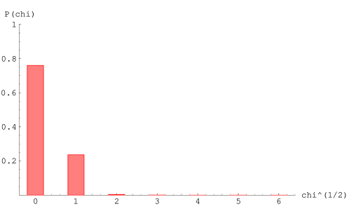
Figure 14: Distribution of the mean chirality $\chi$ in compactification to four dimensions.

A computation of the value of $\chi$ according to (62) for all models leads to a frequency distribution of the mean chirality as shown in figure 14. This distribution is basically identical to the one we obtained in section 3.1.2, shown in figure 11. In particular we also find that models with a mean chirality of $0$ dominate the spectrum and are exponentially more frequent then chiral ones.

From the similarity with the distribution of models on $T^{4}/\mathbb{Z}_{2}$ we can also conjecture that there is a correlation between the mean chirality and the total rank, as we found it to be the case for the six-dimensional models in section 3.1.3. Let us postpone this question to section 3.6, where we give a more detailed account of several questions concerning the correlation of observables.

3.3 Standard model constructions

An important subset of the models considered in the previous section are of course those which could provide a standard model gauge group at low energies. More precisely, since we are dealing with supersymmetric models only, we are looking for models which might resemble the particle spectrum of the MSSM.

To realise the gauge group of the standard model we need generically four stacks of branes (denoted by a,b,c,d) with two possible choices for the gauge groups:

$$U(3)_{a}\times U(2)_{b}\times U(1)_{c}\times U(1)_{d},\quad\mbox{or}\quad U(3)_{a}\times Sp(2)_{b}\times U(1)_{c}\times U(1)_{d}.$$ (63)

To exclude exotic chiral matter from the first two factors we have to impose the constraint that $\#\mathbf{Sym}_{a/b}=0$, i.e. the number of symmetric representations of stacks $a$ and $b$ has to be zero. Models with only three stacks of branes can also be realised, but they suffer generically from having non-standard Yukawa couplings. Since we are not treating our models in so much detail and are more interested in their generic distributions, we include these three-stack constructions in our analysis.

Another important ingredient for standard model-like configurations is the existence of a massless $U(1)_{Y}$ hypercharge. This is in general a combination

$$U(1)_{Y}=\sum_{a=1}^{k}x_{a}U(1)_{a},$$ (64)

including contributions of several $U(1)$s. Since we would like to construct the matter content of the standard model, we are very constrained about the combination of U(1) factors. In order to obtain the right hypercharges for the standard model particles, there are three different combinations of the $U(1)$s used to construct the quarks and leptons possible,

$$U(1)_{Y}^{(1)} = \frac{1}{6}U(1)_{a}+\frac{1}{2}U(1)_{c}+\frac{1}{2}U(1)_{d},$$

$$U(1)_{Y}^{(2)} = -\frac{1}{3}U(1)_{a}-\frac{1}{2}U(1)_{b},$$

$$U(1)_{Y}^{(3)} = -\frac{1}{3}U(1)_{a}-\frac{1}{2}U(1)_{b}+U(1)_{d},$$ (65)

where choices 2 and 3 are only available for the first choice of gauge groups. As explained in section 2.1.4, we can construct a massless combination of $U(1)$ factors, if (11) is satisfied. This gives an additional constraint on the wrapping numbers $\vec{Y}$.

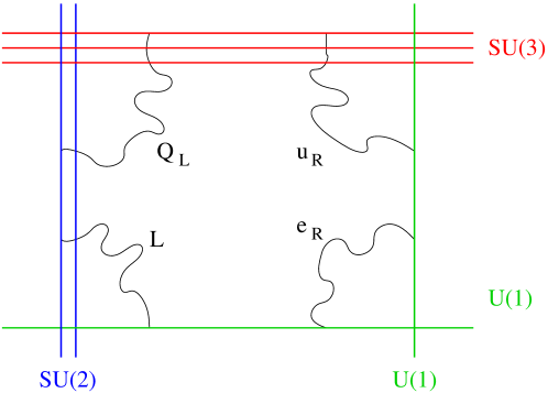
Figure 15: Assignment of brane intersections and chiral matter content for the first of the possible realisations of the standard model using intersecting branes.

For the different possibilities to construct the hypercharge this constraint looks different. In the case of $U(1)_{Y}^{(1)}$ the condition can be formulated as

$$\vec{Y}_{a}+\vec{Y}_{c}+\vec{Y}_{d}=0.$$ (66)

For $Q_{Y}^{(2)}$, where the right-handed up-type quarks are realised as antisymmetric representations of $U(3)$ [3, 18], we obtain

$$\vec{Y}_{a}+\vec{Y}_{b}=0,$$ (67)

and for $Q_{Y}^{(3)}$, where we also need antisymmetric representations of $U(3)$ to realise the right-handed up-quarks, we get

$$\vec{Y}_{a}+\vec{Y}_{b}-\vec{Y}_{d}=0.$$ (68)

In total we have found four ways to realise the standard model with massless hypercharge, summarised with the explicit realisation of the fundamental particles in tables 2 and 3. The chiral matter content arises at the intersection of the four stacks of branes. This is shown schematically for one of the four possibilities in figure 15.

particle	representation	mult.
$U(3)_{a}\times Sp(2)_{b}\times U(1)_{c}\times U(1)_{d}$ with $Q_{Y}^{(1)}$
$Q_{L}$	$(\mathbf{3},\mathbf{2})_{0,0}$	$I_{ab}$
$u_{R}$	$(\overline{\mathbf{3}},\mathbf{1})_{-1,0}+(\overline{\mathbf{3}},\mathbf{1})_{0,-1}$	$I_{a^{\prime}c}+I_{a^{\prime}d}$
$d_{R}$	$(\overline{\mathbf{3}},\mathbf{1})_{1,0}+(\overline{\mathbf{3}},\mathbf{1})_{0,1}$	$I_{a^{\prime}c^{\prime}}+I_{a^{\prime}d^{\prime}}$
$d_{R}$	$(\overline{\mathbf{3}}_{A},\mathbf{1})_{0,0}$	$\frac{1}{2}(I_{aa^{\prime}}+I_{a{\rm O}6})$
$L$	$(\mathbf{1},\mathbf{2})_{-1,0}+(\mathbf{1},\mathbf{2})_{0,-1}$	$I_{bc}+I_{bd}$
$e_{R}$	$(\mathbf{1},\mathbf{1})_{2,0}$	$\frac{1}{2}(I_{cc^{\prime}}-I_{c{\rm O}6})$
$e_{R}$	$(\mathbf{1},\mathbf{1})_{0,2}$	$\frac{1}{2}(I_{dd^{\prime}}-I_{d{\rm O}6})$
$e_{R}$	$(\mathbf{1},\mathbf{1})_{1,1}$	$I_{cd^{\prime}}$
$U(3)_{a}\times U(2)_{b}\times U(1)_{c}\times U(1)_{d}$ with $Q_{Y}^{(1)}$
$Q_{L}$	$(\mathbf{3},\overline{\mathbf{2}})_{0,0}$	$I_{ab}$
$Q_{L}$	$(\mathbf{3},\mathbf{2})_{0,0}$	$I_{ab^{\prime}}$
$u_{R}$	$(\overline{\mathbf{3}},\mathbf{1})_{-1,0}+(\overline{\mathbf{3}},\mathbf{1})_{0,-1}$	$I_{a^{\prime}c}+I_{a^{\prime}d}$
$d_{R}$	$(\overline{\mathbf{3}},\mathbf{1})_{1,0}+(\overline{\mathbf{3}},\mathbf{1})_{0,1}$	$I_{a^{\prime}c^{\prime}}+I_{a^{\prime}d^{\prime}}$
$d_{R}$	$(\overline{\mathbf{3}}_{A},\mathbf{1})_{0,0}$	$\frac{1}{2}(I_{aa^{\prime}}+I_{a{\rm O}6})$
$L$	$(\mathbf{1},\mathbf{2})_{-1,0}+(\mathbf{1},\mathbf{2})_{0,-1}$	$I_{bc}+I_{bd}$
$L$	$(\mathbf{1},\overline{\mathbf{2}})_{-1,0}+(1,\overline{\mathbf{2}})_{0,-1}$	$I_{b^{\prime}c}+I_{b^{\prime}d}$
$e_{R}$	$(\mathbf{1},\mathbf{1})_{2,0}$	$\frac{1}{2}(I_{cc^{\prime}}-I_{c{\rm O}6})$
$e_{R}$	$(\mathbf{1},\mathbf{1})_{0,2}$	$\frac{1}{2}(I_{dd^{\prime}}-I_{d{\rm O}6})$
$e_{R}$	$(\mathbf{1},\mathbf{1})_{1,1}$	$I_{cd^{\prime}}$

Table 2: Realisation of quarks and leptons for the two different choices of gauge groups (63) and hypercharge (1) in (3.3).

particle	representation	mult.
$U(3)_{a}\times U(2)_{b}\times U(1)_{c}\times U(1)_{d}$ with $Q_{Y}^{(2)}$
$Q_{L}$	$(\mathbf{3},\overline{\mathbf{2}})_{0,0}$	$I_{ab}$
$u_{R}$	$(\overline{\mathbf{3}}_{A},\mathbf{1})_{0,0}$	$\frac{1}{2}(I_{aa^{\prime}}+I_{a{\rm O}6})$
$d_{R}$	$(\overline{\mathbf{3}},\mathbf{1})_{-1,0}+(\overline{\mathbf{3}},1)_{0,-1}$	$I_{a^{\prime}c}+I_{a^{\prime}d}$
$d_{R}$	$(\overline{\mathbf{3}},\mathbf{1})_{1,0}+(\overline{\mathbf{3}},1)_{0,1}$	$I_{a^{\prime}c^{\prime}}+I_{a^{\prime}d^{\prime}}$
$L$	$(\mathbf{1},\mathbf{2})_{-1,0}+(\mathbf{1},\mathbf{2})_{0,-1}$	$I_{bc}+I_{bd}$
$L$	$(\mathbf{1},\mathbf{2})_{1,0}+(\mathbf{1},\mathbf{2})_{0,1}$	$I_{bc^{\prime}}+I_{bd^{\prime}}$
$e_{R}$	$(\mathbf{1},\overline{\mathbf{1}}_{A})_{0,0}$	$-\frac{1}{2}(I_{bb^{\prime}}+I_{b{\rm O}6})$
$U(3)_{a}\times U(2)_{b}\times U(1)_{c}\times U(1)_{d}$ with $Q_{Y}^{(3)}$
$Q_{L}$	$(\mathbf{3},\overline{\mathbf{2}})_{0,0}$	$I_{ab}$
$u_{R}$	$(\overline{\mathbf{3}}_{A},\mathbf{1})_{0,0}$	$\frac{1}{2}(I_{aa^{\prime}}+I_{a{\rm O}6})$
$d_{R}$	$(\overline{\mathbf{3}},\mathbf{1})_{-1,0}$	$I_{a^{\prime}c}$
$d_{R}$	$(\overline{\mathbf{3}},\mathbf{1})_{1,0}$	$I_{a^{\prime}c^{\prime}}$
$L$	$(\mathbf{1},\overline{\mathbf{2}})_{0,-1}$	$I_{b^{\prime}d}$
$e_{R}$	$(\mathbf{1},\overline{\mathbf{1}}_{A})_{0,0}$	$-\frac{1}{2}(I_{bb^{\prime}}+I_{b{\rm O}6})$
$e_{R}$	$(\mathbf{1},\mathbf{1})_{1,1}$	$I_{cd^{\prime}}$
$e_{R}$	$(\mathbf{1},\mathbf{1})_{-1,1}$	$I_{c^{\prime}d^{\prime}}$

Table 3: Realisation of quarks and leptons for hypercharges (2) and (3) of (3.3), which can only be realised for the first choice of gauge groups in (63).

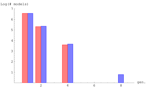
Figure 16: Number of quark and lepton generations with (red bars on the left) and without (blue bars on the right) enforcing a massless $U(1)$.

3.3.1 Number of generations

The first question one would like to ask, after having defined what a ”standard model” is in our setup, concerns the frequency of such configurations in the space of all solutions. Put differently: How many standard models with three generations of quarks and leptons do we find? The answer to this question is zero, even if we relax our constraints and allow for a massive hypercharge (which is rather fishy from a phenomenological point of view). The result of the analysis can be seen in figure 16.

To analyse this result more closely, we relaxed our constraints further and allowed for different numbers of generations for the quark and lepton sector. This is of course phenomenologically no longer relevant, but it helps to understand the structure of the solutions. The three-dimensional plot of this analysis is shown in figure 17. Actually there exist solutions with three generations of either quarks or leptons, where models with only one generation of quarks clearly dominate. The suppression of three generation models can therefore be pinned down to the construction of models with three generations of quarks, which arise at the intersection of the $U(3)$ with the $SU(2)/Sp(2)$ branes and the $U(1)$ branes respectively. models with three generations of either quarks or leptons are shown in table 4.

# of quark gen.	# of lepton gen.	# of models
1	3	183081
2	3	8
3	4	136
4	3	48

Table 4: Number of models found with either three quark or three lepton generations.

This result is rather strange, since we know that models with three families of quarks and leptons have been constructed in our setup (e.g. in [20, 25, 82, 34]). A detailed analysis of the models in the literature shows that all models which are known use (in our conventions) large values for the complex structure variables $U_{I}$ and therefore did not appear in our analysis (see section 2.2.3). On the other hand we know that the number of models decreases exponentially with higher values for the complex structures. Therefore we conclude that standard models with three generations are highly suppressed in this specific setup.

This brings up a natural question, namely: How big is this suppression factor? We postpone this question to section 3.6.2, where we analyse this issue more closely and finally give an estimate for the probability to find a three generation standard model in our setup. For now let us just notice that this probability has to be smaller than the inverse of the total number of models we analysed, i.e. $<10^{-8}$.

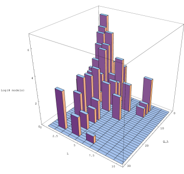
Figure 17: Logarithmic plot of the number of models with different numbers of generations of quarks and leptons. $Q_{L}$ denotes the number of quark families, $L$ is the number of lepton generations.

3.3.2 Hidden sector

Besides the so called “visible sector” of the model, containing the standard model gauge group and particles, we have generically additional chiral matter, transforming under different gauge groups. This sector is usually called the “hidden sector” of the theory, assuming that the masses of the additional particles are lifted and therefore unobservable at low energies.

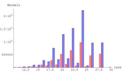
(a)

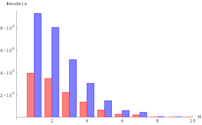
(b)

Figure 18: Frequency distributions of (a) total rank and (b) single gauge group factors in the hidden sector of MSSM-models (red bars on the left) and MSSM models with massive $U(1)$ (blue bars on the right).

In figure 18(a) we show the frequency distributions of the total rank of gauge groups in the hidden sector. In 18(b) we show the frequency distribution of individual gauge group factors. Comparing these results with the distributions of the full set of models in figure 13, we observe that at a qualitative level the restriction to the standard model gauge group in the visible sector did not change the distribution of gauge group observables. The number of constructions in the standard model case is of course much lower, but the frequency distributions of the hidden sector properties behave pretty much like those we obtained for the complete set of models.

As we argue in section 3.6, this is not a coincidence, but a generic feature of the class of models we analysed. Many of the properties of our models can be regarded to be independent of each other, which means that the statistical analysis of the hidden sector of any model with specific visible gauge group leads to very similar results.

3.3.3 Gauge couplings

The gauge sector considered so far belongs to the topological sector of the theory, in the sense that its observables are defined by the wrapping numbers of the branes and independent of the geometric moduli. This does not apply to the gauge couplings, which explicitly do depend on the complex structures, following the derivation in [19], which in our conventions reads

$$\frac{1}{\alpha_{a}}=\frac{M_{Planck}}{2\sqrt{2}M_{s}\kappa_{a}}\,\frac{1}{c\sqrt{\prod_{i=1}^{3}R_{1}^{(i)}R_{2}^{(i)}}}\sum_{I=0}^{3}X^{I}U_{I},$$ (69)

where $\kappa_{a}=1$ or $2$ for an $U(N)$ or $Sp(2N)$ stack respectively.

If one wants to perform an honest analysis of the coupling constants, one would have to compute their values at low energies using the renormalization group equations. We are not going to do this, but look instead at the distribution of $\alpha_{s}/\alpha_{w}$ at the string scale. A value of one at the string scale does of course not necessarily mean unification at lower energies, but it could be taken as a hint in this direction.

To calculate the coupling $\alpha_{Y}$ we have to include contributions from all branes used for the definition of $U(1)_{Y}$. Therefore we need to distinguish the different possible constructions defined in (3.3). In general we have

$$\frac{1}{\alpha_{Y}}=\sum_{a=1}^{k}2N_{a}x_{a}^{2}\frac{1}{\alpha_{a}},$$ (70)

which for the three different possibilities reads explicitly

$$\frac{1}{\alpha_{Y}^{(1)}} = \frac{1}{6}\frac{1}{\alpha_{a}}+\frac{1}{2}\frac{1}{\alpha_{c}}+\frac{1}{2}\frac{1}{\alpha_{d}},$$

$$\frac{1}{\alpha_{Y}^{(2)}} = \frac{2}{3}\frac{1}{\alpha_{a}}+\frac{1}{\alpha_{b}},$$

$$\frac{1}{\alpha_{Y}^{(3)}} = \frac{2}{3}\frac{1}{\alpha_{a}}+\frac{1}{\alpha_{b}}+2\frac{1}{\alpha_{d}}.$$ (71)

The result is shown in figure 19(a) and it turns out that only 2.75% of all models actually do show gauge unification at the string scale.

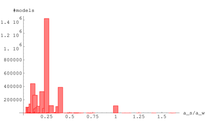
(a)

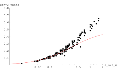
(b)

Figure 19: (a) Frequency distribution of $\alpha_{s}/\alpha_{w}$ in standard model-like configurations. (b) Values of $sin^{2}\theta$ depending on $\alpha_{s}/\alpha_{w}$. Each dot represents a class of models with these values.

Furthermore we analyse the distribution of values for the Weinberg angle

$$\sin^{2}\theta=\frac{\alpha_{Y}}{\alpha_{Y}+\alpha_{w}},$$ (72)

which depends on the ratio $\alpha_{s}/\alpha_{w}$. We want to check the following relation between the three couplings, which was proposed in [19] and is supposed to hold for a large class of intersecting brane models

$$\frac{1}{\alpha_{Y}}=\frac{2}{3}\frac{1}{\alpha_{s}}+\frac{1}{\alpha_{w}}.$$ (73)

From this equation we can derive a relation for the weak mixing angle

$$\sin^{2}\theta=\frac{3}{2}\,\frac{1}{\alpha_{w}/\alpha_{s}+3}.$$ (74)

The result is shown in figure 19(b), where we included a red line that represents the relation (73). The fact that actually 88% of all models obey this relation is a bit obscured by the plot, because each dot represents a class of models and small values for $\alpha_{s}/\alpha_{w}$ are highly preferred, as can be seen from figure 19(a).

3.3.4 Comparison with the statistics of Gepner models

In this paragraph we would like to compare our results with the analysis of [48, 49], where a search for standard model-like features in Gepner model constructions [64, 63, 23, 21] has been performed.

To do so, we have to take only a subset of the data analysed in the previous sections, since the authors of [48, 49] restricted their analysis to a special subset of constructions. Due to the complexity of the problem they restricted their analysis to models with a maximum of three branes in the hidden sector and focussed on three-generation models only. Since the number of generations does not modify the frequency distributions and we obtained no explicit results for three generation models, we include models of an arbitrary number of generations in the analysis. To match the first constraint we filter our results and include only those models with a maximum of three hidden branes. But, as we will see, this does also not change the qualitative behaviour of the frequency distributions.

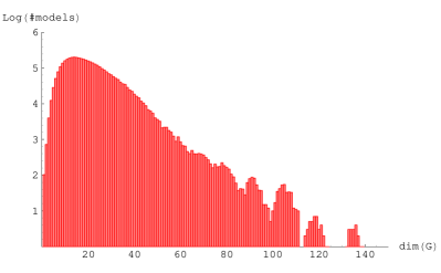
(a)

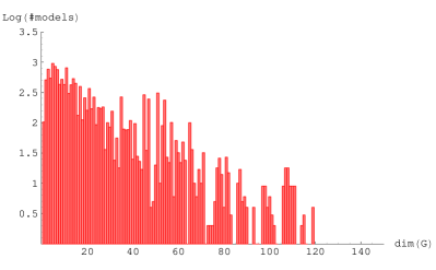
(b)

Figure 20: Frequency distribution of the dimension of the hidden sector gauge group. Figure (a) is the full set of models, figure (b) shows the subset of solutions with a maximum of three branes in the hidden sector.

In figure 20 we show the frequency distribution of the dimension of the hidden sector gauge group before (a) and after (b) the truncation to a maximum of three hidden branes. Obviously the number of models drops significantly, but the qualitative shape of the distribution remains the same. Figure 20(b) can be compared directly with figure 5 of [49]. From a qualitative point of view both distributions are very similar, which could have been expected since the Gepner model construction is from a pure topological point of view quite similar to intersecting D-branes. A major difference can be observed in the absolute values of models analysed. In the Gepner case the authors of [49] found a significantly larger amount of candidates for a standard model.

Besides the frequency distribution of gauge groups we can also compare the analysis of the distribution of gauge couplings. In particular, the distribution of values for for $\sin^{2}\theta$ depending on the ratio $\alpha_{w}/\alpha_{s}$, figure 19(b), can be compared with figure 6 of [49]. We find, in contrast to the case of hidden sector gauge groups, very different distributions. While almost all of our models are distributed along one curve, in the Gepner case a much larger variety of values is possible. The fraction of models obeying (73) was found to be only about 10% in the Gepner model case, which can be identified as a very thin line in figure 6 of [49]. This discrepancy might be traced back to the observation that in contrast to the topological data of gauge groups we are dealing with geometrical aspects here.

As explained in the last paragraph, the gauge couplings do depend explicitly on the geometric moduli. A major difference between the Gepner construction and our intersecting D-brane models lies in the different regimes of internal radius that can be assumed. In our approach we rely on the fact that we are in a perturbative regime, i.e. the compactification radius is much larger than the string length and the string coupling is small.

3.4 Pati-Salam models

As in the case of a $SU(3)\times SU(2)\times U(1)$ gauge group, we can try to construct models with a gauge group of Pati-Salam type

$$SU(4)\times SU(2)_{L}\times SU(2)_{R}.$$ (75)

Analogous to the case of a standard model-like gauge group, we analysed the statistical data for Pati-Salam constructions, realised via the intersection of three stacks of branes. One brane with $N_{a}=4$ and two stacks with $N_{b/c}=2$, such that the chiral matter of the model can be realised as

$$Q_{L}=(\mathbf{4},\mathbf{2},\mathbf{1}),\quad Q_{R}=(\overline{\mathbf{4}},\mathbf{1},\mathbf{2}).$$ (76)

One possibility to obtain the standard model gauge group in this setup is given by breaking the $SU(4)$ into $SU(3)\times U(1)$ and one of the $SU(2)$ groups into $U(1)\times U(1)$. This can be achieved by separating the four branes of stack $a$ into two stacks consisting of three and one branes, respectively, and the two branes of stack $b$ or $c$ into two stacks consisting of one brane each. The separation corresponds to giving a vacuum expectation value to the fields in the adjoint representation of the gauge groups $U(N_{a})$ and $U(N)_{b/c}$, respectively.

Models of this type have been constructed explicitly in the literature, see e.g [38, 37, 35, 33, 34, 29]. However, one has to be careful comparing these models with our results, since our constraints are stronger compared to those usually imposed. In particular, we do not allow for symmetric or antisymmetric representations of $SU(4)$, a constraint that is not always fulfilled for the models that can be found in the references above.

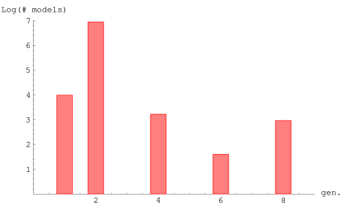
Figure 21: Logarithmic plot of the number of Pati-Salam models found, depending on the number of generations. The solutions have been restricted to an equal number of left- and right-handed fermions, i.e. $gen.=Q_{L}\stackrel{{\scriptstyle!}}{{=}}Q_{R}$

A restriction on the possible models, similar to the standard model case, is provided by the constraint that there should be no additional antisymmetric matter and the number of chiral fermions transforming under $SU(2)_{L}$ and $SU(2)_{R}$ should be equal.

As can be seen in figure 21, we found models with up to eight generations, but no three-generation models. The conclusion is the same as in section 3.3 – the suppression of three generation models is extremely large and explicit models show up only at very large values of the complex structure parameters. The distribution differs from the standard model case in the domination of two-generation models. This is an interesting phenomenon, which can be traced back to the specific construction of the models using two $N=2$ stacks of branes. This example shows that the number of generations, in contrast to the distribution of gauge groups in the hidden sector (see also section 3.6), does depend on the specific visible sector gauge group we chose.

3.5 SU(5) models

From a phenomenological point of view a very interesting class of low-energy models consist of those with a grand unified gauge group, providing a framework for the unification of the strong and electro-weak forces.

The minimal simple Lie group that could be used to achieve this is $SU(5)$ [62] or also the so-called flipped $SU(5)$ [11, 43], consisting of the gauge group $SU(5)\times U(1)_{X}$. They represent the two possibilities how to embed an $SU(5)$ gauge group into $SO(10)$. The flipped construction is more interesting phenomenologically, because models based on this gauge group might survive the experimental limits on proton decay. Several explicit constructions of supersymmetric $SU(5)$ models in the context of intersecting D-brane models are present in the literature [36, 7, 27, 26, 30, 28], as well as some non-supersymmetric ones [18, 59].

In the remainder of this section we present some results on the distribution of the gauge group properties of $SU(5)$ and flipped $SU(5)$ models, using the same $T^{6}/\mathbb{Z}_{2}\!\times\!\mathbb{Z}_{2}$ orientifold setting as in the previous sections. This part is based on [71].

3.5.1 Construction

In the original $SU(5)$ construction, the standard model particles are embedded in a $\mathbf{\bar{5}}$ and a $\mathbf{10}$ representation of the unified gauge group as follows

$$SU(5) \to SU(3)\times SU(2)\times U(1)_{Y},$$

$$\mathbf{\bar{5}} \to (\mathbf{\bar{3}},\mathbf{1})_{2/3}+(\mathbf{1},\mathbf{2})_{-1},$$

$$\mathbf{10} \to (\mathbf{\bar{3}},\mathbf{1})_{-4/3}+(\mathbf{3},\mathbf{2})_{1/3}+(\mathbf{1},\mathbf{1})_{2},$$ (77)

where the hypercharge is generated by the $SU(3)\times SU(2)$-invariant generator

$$Z=\mathrm{diag}(-1/3,-1/3,-1/3,1/2,1/2).$$ (78)

In the flipped $SU(5)$ construction, the embedding is given by

$$SU(5)\times U(1)_{X} \to SU(3)\times SU(2)\times U(1)_{Y},$$

$$\mathbf{\bar{5}}_{-3} \to (\mathbf{\bar{3}},\mathbf{1})_{-4/3}+(\mathbf{1},\mathbf{2})_{-1},$$

$$\mathbf{10}_{1} \to (\mathbf{\bar{3}},\mathbf{1})_{2/3}+(\mathbf{3},\mathbf{2})_{1/3}+(\mathbf{1},\mathbf{1})_{0},$$

$$\mathbf{1}_{5} \to (\mathbf{1},\mathbf{1})_{2},$$ (79)

including a right-handed neutrino $(\mathbf{1},\mathbf{1})_{0}$. The hypercharge is in this case given by the combination

$$Y=-\frac{2}{5}Z+\frac{2}{5}X.$$ (80)

We would like to realise models of both type within our orientifold setup. The $SU(5)$ case is simpler, since in principle it requires only two branes, a $U(5)$ brane $a$ and a $U(1)$ brane $b$, which intersect such that we get the $\mathbf{\bar{5}}$ representation at the intersection. The $\mathbf{10}$ is realised as the antisymmetric representation of the $U(5)$ brane. To get reasonable models, we have to require that the number of antisymmetric representations is equal to the number of $\mathbf{\bar{5}}$ representations,

$$I_{ab}=-\#\mathbf{Anti}_{a}.$$ (81)

In a pure $SU(5)$ model one should also include a restriction to configurations with $\#\mathbf{Sym}_{a}=0$ to exclude $\mathbf{15}$ representations from the beginning. Since it has been proven in [36] that in this case no three generation models can be constructed and symmetric representations might also be interesting from a phenomenological point of view, we include these in our discussion.

The flipped $SU(5)$ case is a bit more involved since in addition to the constraints of the $SU(5)$ case one has to make sure that the $U(1)_{X}$ stays massless and the $\mathbf{\bar{5}}$ and $\mathbf{10}$ have the right charges, summarised in (3.5.1). To achieve this, at least one additional brane $c$ is needed. Generically, the $U(1)_{X}$ can be constructed as a combination of all $U(1)$s present in the model

$$U(1)_{X}=\sum_{a=1}^{k}x_{a}U(1)_{a}.$$ (82)

The simplest way to construct a combination which gives the right charges would be

$$U(1)_{X}=\frac{1}{2}U(1)_{a}-\frac{5}{2}U(1)_{b}+\frac{5}{2}U(1)_{c},$$ (83)

but a deeper analysis shows [96], that this is in almost all cases not enough to ensure that the hypercharge remains massless. The condition for this can be formulated as

$$\sum_{a=1}^{k}x_{a}N_{a}\vec{Y}_{a}=0,$$ (84)

with the coefficients $x_{a}$ from (83). To fulfill this requirement we need generically one or more additional $U(1)$ factors.

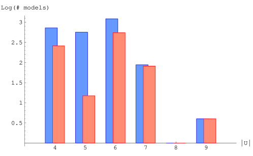
Figure 22: Logarithmic plot of the number of solutions with an $SU(5)$ factor depending on the absolute value of the parameters $U$. We give the results with (blue bars to the left) and without (red bars to the right) symmetric representations of $SU(5)$.

3.5.2 General results

Having specified the additional constraints, we use the techniques described in section 2.2.3 to generate as many solutions to the tadpole, supersymmetry and K-theory conditions as possible. The requirement of a specific set of branes to generate the $SU(5)$ or flipped $SU(5)$ simplifies the computation and gives us the possibility to explore a larger part of the moduli space as compared to the more general analysis we described above.

Before doing an analysis of the gauge sector properties of the models under consideration, we would like to check if the number of solutions decreases exponentially for large values of the $U_{I}$, as we observed in section 3.2.1 for the general solutions. In figure 22 the number of solutions with and without symmetric representations are shown. The scaling holds in our present case as well, although the result is a bit obscured by the much smaller statistics. In total we found 2590 solutions without restrictions on the number of generations and the presence of symmetric representations. Excluding these representations reduces the number of solutions to 914. Looking at the flipped $SU(5)$ models, we found 2600 with and 448 without symmetric representations. Demanding the absence of symmetric representations is obviously a much severer constraint in the flipped case.

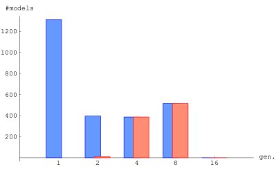
(a)

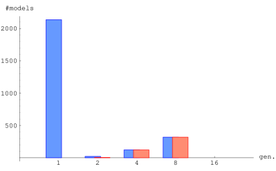
(b)

Figure 23: Plots of the number of solutions for different numbers of generations for (a) $SU(5)$ and (b) flipped $SU(5)$ models with (blue bars to the left) and without (red bars to the right) symmetric representations of $SU(5)$.

The correct number of generations turned out to be the strongest constraint on the statistics in our previous work on standard model constructions. The $SU(5)$ case is not different in this aspect. In figure 23 we show the number of solutions for different numbers of generations. We did not find any solutions with three $\mathbf{\bar{5}}$ and $\mathbf{10}$ representations. This situation is very similar to the one we encountered in our previous analysis of models with a standard model gauge group in section 3.3. An analysis of the models which have been explicitly constructed showed that they exist only for very large values of the complex structure parameters. The same is true in the present case. Because the number of models decreases rapidly for higher values of the parameters, we can draw the conclusion that these models are statistically heavily suppressed.

Comparing the standard and the flipped $SU(5)$ construction the result for models with one generation might be surprising, since there are more one generation models in the flipped than in the standard case. This is due to the fact that there are generically different possibilities to realise the additional $U(1)_{X}$ factor for one geometrical setup, which we counted as distinct models.

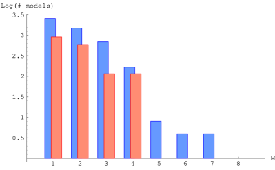
(a)

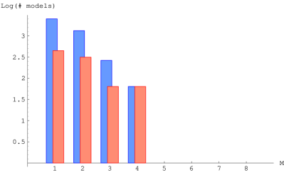
(b)

Figure 24: Logarithmic plots of the number of solutions with a specific rank $M$ gauge factor in the hidden sector in (a) $SU(5)$ and (b) flipped $SU(5)$ models with (blue bars to the left) and without (red bars to the right) symmetric representations of $SU(5)$.

Regarding the hidden sector, we found in total only four $SU(5)$ models which did not have a hidden sector at all - one with 4, two with 8 and one with 16 generations. For the flipped $SU(5)$ case such a model cannot exist, because it is not possible to solve the condition for a massless $U(1)_{X}$ without hidden sector gauge fields.

The frequency distribution of properties of the hidden sector gauge group, the probability to find a gauge group of specific rank $M$ and the distribution of the total rank, are shown in figures 24 and 25. The distribution for individual gauge factors is qualitatively very similar to the one obtained for all possible solutions above (see figures 13). One remarkable difference between standard and flipped $SU(5)$ models is the lower probability for higher rank gauge groups. This is due to the above mentioned necessity to have a sufficient number of hidden branes for the construction of a massless $U(1)_{X}$.

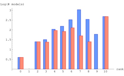
(a)

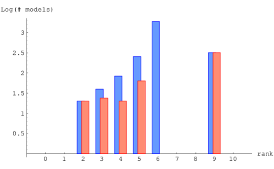
(b)

Figure 25: Plots of the number of solutions for given values of the total rank of the hidden sector gauge group in (a) $SU(5)$ and (b) flipped $SU(5)$ models with (blue bars to the left) and without (red bars to the right) symmetric representations of $SU(5)$.

The total rank distribution for both, the standard and the flipped version, differs in one aspect from the one obtained in 3.2.1, namely in the large fraction of hidden sector groups with a total rank of 10 or 9, respectively. This can be explained by just one specific construction which is possible for various values of the complex structure parameters. In this setup the hidden sector branes are all except one on top the orientifold planes on all three tori. If we exclude this specific feature of the $SU(5)$ construction, the remaining distribution shows the behaviour estimated from the prior results.

Note that while comparing the distributions one has to take into account that the total rank of the hidden sector gauge group in the $SU(5)$ case is lowered by the contribution from the visible sector branes to the tadpole cancellation conditions. In the flipped case, the additional $U(1)$-brane contributes as well.

3.5.3 Restriction to three branes in the hidden sector

In order to compare our results for the statistics of constructions with a standard model-like gauge group with Gepner models in section 3.3.4, we truncated the full set of models to those with only three stacks of branes in the hidden sector. In the following we also perform a restriction to a maximum of three branes in the hidden sector in the $SU(5)$ case, but with a different motivation and in a different way. We do not truncate our original results, but instead impose the constraint to a maximum of three branes from the very beginning in the computational process. It turns out that such a restriction can greatly improve the performance of the partition algorithm and allows us therefore to analyse a much bigger range of complex structures. This is highly desirable, since it opens up the possibility to check some claims about the growths of solutions that we made in section 2.3. The method has also some drawbacks. Since we do not compute the full distribution of models, but with an artificial cutoff, we can not be sure that the frequency distributions of properties in the gauge sector are the same as in the full set of models. As we will see in the following, there are indeed some deviations.

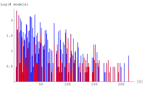
Figure 26: Logarithmic plot of the number of solutions with an $SU(5)$ factor depending on the absolute value of the parameters $U$. The number of brane stacks in the hidden sector is restricted to three and the results are shown for models with (blue spikes) and without (red spikes) symmetric representations of $SU(5)$.

In figure 26 we plotted the total number of models with a maximum of three stacks of branes in the hidden sector. As in our analysis above we show the models without symmetric representations separately. This plot should be compared with figure 22, the number of solutions for $SU(5)$ models without restrictions. In the restricted case we were able to compute up to much higher values of the complex structures and confirm the assertion of 2.3, that the number of solution drops exponentially with $|U|$. This provides another hint that the total number of solutions is indeed finite. In total we found 3275 solutions, which is more then in the case without restrictions, but in contrast to a range of complex structures which is 25 times bigger, the amount of additional solutions is comparably small.

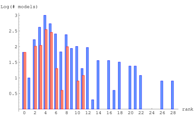
(a)

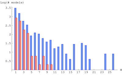
(b)

Figure 27: Logarithmic plots of the frequency distributions in the hidden sector of $SU(5)$ models with a maximum of three hidden branes. (a) Specific rank $M$ gauge factors, (b) Total rank of the hidden sector gauge group.

Comparing the distributions for individual gauge factors (figure 27(a)) and the total rank in the hidden sector (figure 27(b)), we see some interesting differences to figures 24(a) and 25(a). The distribution of individual gauge factors is just extended to higher factors in the restricted case. This was to be expected, since larger values for the complex structure parameters allow for larger gauge factors to occur, since they provide us with very long branes with negative wrapping numbers $X$ that can compensate these large numbers in the tadpole cancellation conditions. The general shape of the distribution remains unchanged. In the case of the total rank the situation is different. The distribution also shows larger values for the total rank, which is directly correlated to the larger individual ranks of the factors, but moreover the maximum of the distribution is shifted from around seven in the unrestricted case to about four. This can be explained by the fact that the restriction to a maximum of three branes in the hidden sector also restricts the possible contributions from models with many gauge factors of small rank, especially the contribution of $U(1)$ gauge factors.

What about models with a flipped $SU(5)$ gauge group? Repeating the analysis for these models in the case of a restriction in the hidden sector can of course be done, be the results might not be very predictive. For a consistent flipped $SU(5)$ model, we need a massless $U(1)_{X}$, which also depends on a combination of $U(1)$ factors from the hidden sector. After choosing an additional $U(1)$ brane for the visible sector of flipped $SU(5)$ there remain only two hidden sector branes. This restriction is too drastic to give meaningful results, since it turned out in the analysis of flipped $SU(5)$ models that we need more than two hidden sector branes to solve the equations for the $U(1)_{X}$ to be massless.

The analysis in this section showed that three generation models with a minimal grand unified gauge group are heavily suppressed in this specific orientifold setup. This result was expected, since we know that the explicit construction of three generation $SU(5)$ models using the $\mathbb{Z}_{2}\!\times\!\mathbb{Z}_{2}$ orbifold has turned out to be difficult.

The analysis of the hidden sector showed that the frequency distributions of the total rank of the gauge group and of single gauge group factors are quite similar to the results for generic models in section 3.2.1. Differences in the qualitative picture result from specific effects in the $SU(5)$ construction.

Comparing the results for the standard and flipped $SU(5)$ models, we find no significant differences. If we allow for symmetric representations, there is basically no additional suppression factor. If we restrict ourselves to models without these representations, flipped constructions are three times less likely then the standard ones.

3.6 Correlations

An interesting question that we raised in the introduction concerns the correlation of observables. If different properties of our models were correlated, independently of the specific visible gauge group, this would provide us with some information about the generic behaviour of this class of models. In the following discussion we would like to clarify this point, emphasizing a crucial difference between correlations of phenomenologically interesting observables in the gauge sector of our models on the one hand, and correlations between basic properties used as constraints to characterize a specific visible sector on the other hand. Finally we use the observations on the second class of correlations to estimate the number of models with a standard model gauge group and three generations of quarks and leptons for the $T^{6}/\mathbb{Z}_{2}\!\times\!\mathbb{Z}_{2}$ orientifold.

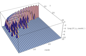
(a)

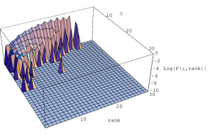
(b)

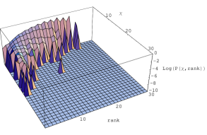
(c)

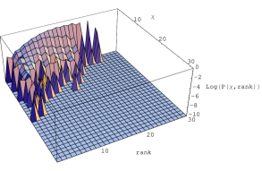
(d)

Figure 28: Logarithmic plots of the relative frequency distributions of models with specific total rank of the gauge group and mean chirality. Plot (a) shows the analysis for the full gauge group of all models, figures (b), (c) and (d) give the results for the hidden sector gauge groups of standard model-like constructions with and without a massive hypercharge and Pati-Salam models, respectively.

3.6.1 Rank and chirality

To give an example of correlations between gauge group observables let us consider the mean chirality $\chi$, defined by (62), and the total rank of the gauge group. As we already saw using the saddle point approximation on $T^{4}$ in section 3.1.3, these two quantities should be correlated. To confirm this in the four-dimensional case, we use our explicit results and compute the frequency distributions for the different visible sectors considered above, standard model-like constructions with and without a massless hypercharge and Pati-Salam models. The result is shown in figure 28. Please note that we have normalised the distributions in order to make the results better comparable.

We find two striking results here, which illustrate the two points we made in the introduction to this section. Firstly the two observables are clearly correlated, a large value for the mean chirality is much more likely to find if the total rank is small. Secondly the results for the full set of models, figure 28(a), and the different visible sectors, figures 28(b), (c) and (d), show qualitatively very similar results. This last observation is intriguing, since we might use this to conjecture that the specific properties used to define an individual visible sector do not influence the distributions. Put differently, we might speculate that these properties could be regarded independent of each other. If this would be indeed the case, it could simplify some specific analysis dramatically. Instead of constructing solutions for one specific setup with some set of properties it would be enough to know the probabilities for each property. Since they would be independent of each other we could just multiply the results and get an answer to our more difficult question.

3.6.2 Estimates

We would like to test this conjecture using the properties of a standard model construction. These include several constraints on the models, in particular the existence of specific $U(N)$ gauge factors, the vanishing of antisymmetric representations, a massless hypercharge and three generations of chiral matter. How can we check whether two of these properties $A$ and $B$, are independent? A good measure for this would be to calculate the correlation between the probabilities $P(A)$ and $P(B)$ to find these properties. This can be expressed as

$$P_{AB}=\frac{P(A)P(B)-P(A\wedge B)}{P(A)P(B)+P(A\wedge B)},$$ (85)

where $P(A\wedge B)$ is the probability to find both properties realised at the same time.

(a)

(b)

Figure 29: Correlations between properties of standard model-like configurations. (a) Correlation between the existence of an $SU(3)$ and an $SU(2)$ or $Sp(2)$ gauge group. (b) Correlation between the existence of an $SU(3)$ gauge group and the absence of symmetric representations.

For concreteness let us take the following properties as examples: The existence of a $U(3)$ gauge group, existence of a $U(2)$ or $Sp(2)$ gauge group and the vanishing of antisymmetric representations. In figure 29 we plotted the value of $P_{AB}$ in the set of all models for different values of the number of stacks. As can be derived from these plots the two properties are not really independent, but values of about $0.1$ and $0.2$, respectively, which are also the order of magnitude for other possible correlations, suggest that one could give it a try and treat these properties as independent in an estimate.

Restriction	Factor
gauge factor $U(3)$	$0.0816$
gauge factor $U(2)/Sp(2)$	$0.992$
No symmetric representations	$0.839$
Massless $U(1)_{Y}$	$0.423$
Three generations of quarks	$2.92\times 10^{-5}$
Three generations of leptons	$1.62\times 10^{-3}$
Total	$1.3\times 10^{-9}$

Table 5: Suppression factors for various constraints of standard model properties.

In table 5 we summarised the properties of a three-generation standard model, including the suppression factor calculated using the probability to find this property in the set of all models and their total number, $1.66\times 10^{8}$. The two $U(1)$ gauge groups required for a standard model setup are not included in this, since the probability to find a $U(1)$ in one of the constructions is essentially one. Multiplying all these factors, we get a probability of $\approx\,1.3\times 10^{-9}$, i.e. one in a billion, to find a three-generation standard model in the $T^{6}/\mathbb{Z}_{2}\!\times\!\mathbb{Z}_{2}$ setup.

How reliable is this estimate? This is of course an important question, since we concluded from the analysis above that the basic properties are only approximately independent and we can not really make a quantitative statement about the possible error in our estimate. So let us compare the result we obtain with this method for models with standard model gauge group and two or four generations of quarks and leptons with the actual numerical results we have obtained in these cases.

The result is shown in table 6. As can be read of this table, the estimate for the two- and four-generation case deviates by around 20% from the correct value. Keeping this in mind and further noting that we are making an estimate only at an order-of-magnitude level, a suppression factor of $\approx 10^{-9}$ seems to be a reliable value.

# generations	# of models found	estimated #	suppression factor
$2$	$162921$	$188908$	$\approx 10^{-3}$
$3$	$0$	$0.2$	$\approx 10^{-9}$
$4$	$3898$	$3310$	$\approx 2\times 10^{-5}$

Table 6: Comparison between the estimated number of solutions and the actual number of solutions found for models with two, three and four generations.

4 Conclusions and outlook

In this work we have reviewed the results on the statistics of the gauge sector of a specific class of orientifold models. We have presented two different methods to derive these results. The saddle point approximation [17], working well in the eight- and six-dimensional case, is not powerful enough to deal with four-dimensional compactifications, forcing us to perform a more direct computer aided analysis [69]. Using this approach, we discussed various aspects of frequency distributions in the gauge sector. After exploring the most general case, we focused on models containing phenomenologically interesting gauge groups. In the particular case of a standard model gauge group [68], an estimate of the number of three generation models in this setup was given, using the fact that the basic properties of such a model are sufficiently uncorrelated. For this class of models we also analysed the values of the gauge couplings at the string scale. In the case of models containing a Pati-Salam or $SU(5)$ gauge group [71], it was shown that the frequency distributions of gauge factors do not change, indicating that the specific choice of a visible sector does not alter the statistics.

Concerning the universality of these results, it should be stressed that it is very likely that some of them depend strongly on the specific geometry that has been chosen. The comparison of some of our results with a study of Gepner models [48] confirms this conjecture, showing that only those results show similarities, which are fairly independent of the geometry. Especially the amount of three generation standard models might be very different if one chooses other orbifold groups. To illuminate this point, a study of models on $T^{6}/\mathbb{Z}_{6}$ is currently under way [70]. It would be of course very desirable to do similar studies in other corners of the landscape, in order to see whether the distribution of models resembling our four dimensional world is uniform or rather sharply peaked at special points in moduli space.

Interesting directions of future studies would be on the one hand to include fluxes in our discussion, which probably give rise to a much larger set of models. On the other hand one could try to obtain frequency distributions of other important aspects of the (supersymmetric) standard model, such as Yukawa couplings or soft supersymmetry breaking terms. Including these in our discussion will certainly reduce the number of acceptable models and might also give additional hints which parts of the landscape are worth to be investigated in greater detail.

Appendix A Orientifold models

In this appendix we summarise the concrete examples of orientifold models that are used in this paper. We fix the notation and translate the conditions explained in general in section 2.1 into variables that suit the specific cases and simplify the computations.

A.1 $\mathbf{T^{2}}$

For compactification on $T^{2}$, a special Lagrangian submanifold is specified by two wrapping numbers $(n_{a},m_{a})$ around the fundamental one-cycles. In this case these numbers are precisely identical to the numbers $(X_{a},Y_{a})$ used in section 2.1.

The tadpole cancellation condition (6) reads

$$\sum_{a}N_{a}\,X_{a}=L,$$ (86)

where the physical value is $L=16$.

The first supersymmetry condition of (7) reads just

$$Y_{a}=0,$$ (87)

and is independent of the complex structure $U=R_{2}/R_{1}$ on the rectangular torus. This implies that all supersymmetric branes must lie along the x-axis, i.e. on top of the orientifold plane. The second supersymmetry condition in (7) becomes

$$X_{a}>0.$$ (88)

From these conditions we can immediately deduce that if one does not allow for multiple wrapping, as it is usually done in this framework, there would only exist one supersymmetric brane, namely the one with $(X,Y)=(1,0)$.

A.2 $\mathbf{T^{4}/\mathbb{Z}_{2}}$

In this case a class of special Lagrangian branes is given by so-called factorisable branes, which can be defined by two pairs of wrapping numbers $(n_{i},m_{i})$ on two $T^{2}$s. The wrapping numbers $(X^{i},Y^{i})$ with $i=1,2$ for the $\mathbb{Z}_{2}$ invariant two-dimensional cycles are then given by

$$X^{1}=n_{1}\,n_{2},\quad\quad X^{2}=m_{1}\,m_{2},\quad\quad Y^{1}=n_{1}\,m_{2},\quad\quad Y^{2}=m_{1}\,n_{2}.$$ (89)

To simplify matters we sometimes use a vector notation $\vec{X}=(X^{1},X^{2})^{T}$ and $\vec{Y}=(X^{1},X^{2})^{T}$.

Note that these branes do not wrap the most general homological class, for the 2-cycle wrapping numbers satisfy the relation

$$X^{1}\,X^{2}=Y^{1}\,Y^{2}.$$ (90)

However, for a more general class we do not know how the special Lagrangians look like. Via brane recombination it is known that there exist flat directions in the D-brane moduli space, corresponding to branes wrapping non-flat special Lagrangians. Avoiding these complications, we use the well understood branes introduced above only.

The untwisted tadpole cancellation conditions read

$$\sum_{a}N_{a}\,X^{1}_{a}=L^{1},\qquad\sum_{a}N_{a}\,X^{2}_{a}=-L^{2},$$ (91)

with the physical values $L_{1}=L_{2}=8$. In order to put these equations on the same footing, we change the sign of $X_{2}$ to get

$$\sum_{a}N_{a}\,X^{1}_{a}=L^{1},\qquad\sum_{a}N_{a}\,X^{2}_{a}=L^{2}.$$ (92)

Note that in contrast to models discussed for example in [65], we are only considering bulk branes without any twisted sector contribution for simplicity. Defining the two form $\Omega_{2}=(dx_{1}+iU_{1}dy_{1})(dx_{2}+iU_{2}dy_{2})$, the supersymmetry conditions become

$$U_{1}\,Y^{1}+U_{2}\,Y^{2}=0,\qquad X^{1}+U_{1}\,U_{2}\,X^{2}>0.$$ (93)

The intersection number between two bulk branes has an extra factor of two

$$I_{ab}=-2\left(X^{1}_{a}\,X^{2}_{b}+X^{a}_{2}\,X^{1}_{b}+Y^{1}_{a}\,Y^{2}_{b}+Y^{2}_{a}\,Y^{1}_{b}\right).$$ (94)

A.2.1 Multiple wrapping

In the case of $T^{2}$ it made no sense to restrict the analysis of supersymmetric branes to those which are not multiply wrapped around the torus, because there would have been just one possible construction. In the case of $T^{4}/\mathbb{Z}_{2}$ the situation is different and we would like to derive the constraints on the wrapping numbers $\vec{X}$ and $\vec{Y}$.

For the original wrapping numbers $n_{i},m_{i}$ the constraint to forbid multiple wrapping is $\gcd(n_{i},m_{i})=1\,\,\forall\,i=1,2$. Without losing information we can multiply these two to get

$$\gcd(n_{1},m_{1})\gcd(n_{2},m_{2})=1.$$ (95)

Using the definitions (89) of $\vec{X}$ and $\vec{Y}$, we can rewrite this as

$$\gcd(X^{1},Y^{2})\gcd(X^{2},Y^{2})=Y_{2},$$ (96)

which is invariant under an exchange of $X$ and $Y$.

A.3 $\mathbf{T^{6}/\mathbb{Z}_{2}\!\times\!\mathbb{Z}_{2}}$

In the case of compactifications on this six-dimensional orientifold, which has been studied by many authors (see e.g. [61, 38, 37, 80, 57, 16]) the situation is very similar to the four-dimensional case above. We can describe factorisable branes by their wrapping numbers $(n_{i},m_{i})$ along the basic one-cycles $\pi_{2i-1},\pi_{2i}$ of the three two-tori $T^{6}=\Pi_{i=1}^{3}T_{i}^{2}$. To preserve the symmetry generated by the orientifold projection $\Omega\bar{\sigma}$, only two different shapes of tori are possible, which can be parametrised by $b_{i}\in\{0,1/2\}$ and transform as

$$\Omega\bar{\sigma}:\left\{\begin{array}[]{rcl}\pi_{2i-1}&\to&\pi_{2i-1}-2b_{i}\pi_{2i}\\ \pi_{2i}&\to&-\pi_{2i}\end{array}\right..$$ (97)

For convenience we work with the combination $\tilde{\pi}_{2i-1}=\pi_{2i-1}-b_{i}\pi_{2i}$ and modified wrapping numbers $\tilde{m}_{i}=m_{i}+b_{i}n_{i}$. Furthermore we introduce a rescaling factor

$$c:=\left(\prod_{i=1}^{3}(1-b_{i})\right)^{-1}$$ (98)

to get integer-valued coefficients. These are explicitly given by ($i,j,k\in\{1,2,3\}$ cyclic)

$$X^{0}=cn_{1}n_{2}n_{3}, X^{i}=-cn_{i}\tilde{m}_{j}\tilde{m}_{k},$$

$$Y^{0}=c\tilde{m}_{1}\tilde{m}_{2}\tilde{m}_{3}, Y^{i}=-c\tilde{m}_{i}n_{j}n_{k}.$$ (99)

The wrapping numbers $\vec{X}$ and $\vec{Y}$ are not independent, but satisfy the following relations:

$$\begin{array}[]{rclcrcl}X_{I}\,Y_{I}&=&X_{J}\,Y_{J},&&X_{L}\,(Y_{L})^{2}&=&X_{I}\,X_{J}\,X_{K},\\ X_{I}\,X_{J}&=&Y_{K}\,Y_{L},&&Y_{L}\,(X_{L})^{2}&=&Y_{I}\,Y_{J}\,Y_{K},\end{array}$$ (100)

for all $I,J,K,L\in\{0,\ldots 3\}$ cyclic.

Using these conventions the intersection numbers can be written as

$$I_{ab}=\frac{1}{c^{2}}\left(\vec{X}_{a}\vec{Y}_{b}-\vec{X}_{b}\vec{Y}_{a}\right).$$ (101)

The tadpole cancellation conditions read

$$\sum_{a=1}^{k}N_{a}\vec{X}_{a}=\vec{L},\quad\quad\vec{L}=\begin{pmatrix}8c\\ \{8/(1-b_{i})\}\end{pmatrix},$$ (102)

where we used that the value of the physical orientifold charge is $8$ in our conventions.

The supersymmetry conditions can be written as

$$\sum_{I=0}^{3}\frac{Y^{I}}{U_{I}}=0,\qquad\sum_{I=0}^{3}X^{I}U_{I}>0,$$ (103)

where we used that the complex structure moduli $U_{I}$ can be defined in terms of the radii $(R_{i}^{(1)},R_{I}^{(2)})$ of the three tori as

$$U_{0} = R_{1}^{(1)}R_{1}^{(2)}R_{1}^{(3)},$$

$$U_{i} = R_{1}^{(i)}R_{2}^{(j)}R_{2}^{(k)},\quad i,j,k\in\{1,2,3\}\,\mbox{cyclic}.$$ (104)

Finally the K-theory constraints can be expressed as

$$\sum_{a=1}^{k}N_{a}Y_{a}^{0}\in 2\mathbb{Z},\quad\quad\frac{1-b_{i}}{c}\sum_{a=1}^{k}N_{a}Y_{a}^{i}\in 2\mathbb{Z},\quad i\in\{1,2,3\}.$$ (105)

A.3.1 Multiple wrapping

We can define the condition to exclude multiple wrapping in a way similar to the $T^{4}$-case. A complication that arises is the possibility to have tilted tori. In the definition of $\vec{X}$ and $\vec{Y}$ in (A.3) we used the wrapping numbers $\tilde{m}_{i}$, which have been defined to include the possible tilt. To analyse coprime wrapping numbers, however, we have to deal with the original wrapping numbers $m_{i}$, such that

$$\prod_{i=1}^{3}\gcd(n_{i},m_{i})=1.$$ (106)

We can express this condition in terms of the variables $\vec{\tilde{X}}$ and $\vec{\tilde{Y}}$, defined as

$$\tilde{X}^{0}=n_{1}n_{2}n_{3}, \tilde{Y}^{0}=m_{1}m_{2}m_{3},$$

$$\tilde{X}^{i}=n_{i}n_{j}n_{k}, \tilde{Y}^{i}=m_{i}n_{j}n_{k},$$ (107)

where $i,j,k\in\{1,2,3\}$ cyclic, analogous to section A.2.1

$$\prod_{i=1}^{3}\gcd(\tilde{Y}^{0},\tilde{X}^{i})=(\tilde{Y}^{0})^{2}.$$ (108)

The $\vec{\tilde{X}}$ and $\vec{\tilde{Y}}$ can be expressed in terms of the $\vec{X}$ and $\vec{Y}$ of (A.3), using their definition (106) and the rescaling factor (98), as

$$\tilde{X}^{0} = c^{-1}X^{0},$$

$$\tilde{X}^{i} = c^{-1}\left(-X^{i}+b_{j}Y^{k}+b_{k}Y^{j}+b_{j}b_{k}X^{0}\right),$$

$$\tilde{Y}^{0} = c^{-1}\left(Y^{0}+\sum_{i=1}^{3}b_{i}X^{i}-\sum_{i=1}^{3}b_{j}b_{k}Y^{i}-b_{1}b_{2}b_{3}X^{0}\right),$$

$$\tilde{Y}^{i} = c^{-1}\left(-Y^{i}-b_{i}X^{0}\right).$$ (109)

Appendix B Partition algorithm

In this part of the appendix we briefly outline the partition algorithm used in the computer analysis of vacua. It is designed to calculate the unordered partition of a natural number $n$, restricted to a maximal number of $m$ factors, using only a subset $F\subset\mathbb{N}$ of allowed factors to appear in the partition.

To describe the main idea, let us drop the additional constraints on the length and factors of the partition. They can be added easily to the algorithm, for details see the comments in listing 2. The result is stored in a list $\{a_{i}\}$, which is initialized with $a_{i}=n\delta_{1,i}$. An internal pointer $q$ is set to the first element at the beginning and after each call of the main routine the list $a$ contains the next partition. The length of this partition is stored in a variable $m$, which is set to $m=0$, after the last partition has been generated.

The main routine contains the following steps. It checks if the element $a_{q}$ is equal to $1$ – if yes, it sets $q=q-1$. This is repeated until $a_{q}>1$ or $q=0$ – in this case no new partitions exist, $m$ is set to $0$ and the algorithm terminates. In the second step the routine sets $a_{q}=a_{q}-1$, $a_{q+1}=a_{q+1}+1$ and $q=q+1$. But this operation is only performed if $a_{q+1}<a_{q}$ and $a_{q}>1$, otherwise the counter $q$ is reduced by one and the algorithm starts over.

Let us give an example to illustrate this procedure. Consider the unordered partitions of $5$:

$$\left\{\,\{5\},\{4,1\},\{3,2\},\{3,1,1\},\{2,2,1\},\{2,1,1,1\},\{1,1,1,1,1\}\,\right\}.$$ (110)

Starting with $5$ itself, the first time we call the algorithm, it decreases $a_{1}$ to $a_{1}=4$, increases $a_{2}$ to $a_{2}=1$, which generates the partition $\{4,1\}$. The pointer $q$ is increased to $q=2$. The next time we call the routine, the element $a_{q}=a_{2}$ is equal to $1$, which leads to $q=1$. Now the condition $a_{q}>1$ is satisfied and the result of $a_{q}=a_{q}-1$, $a_{q+1}=a_{q+1}+1$ gives the partition $\{3,2\}$. Continuing in this way, four more partitions of $5$ are generated, until we reach $\{1,1,1,1,1\}$. We have $a_{i}=1$ for all $i=1,\ldots,5$, which leads to the termination of the algorithm in the first step.

B.1 Implementation

The algorithm uses a data structure partition to collect the necessary parameters and internal variables:

⬇

typedef struct _partition { long n,m,q,*fac,*a,min; } partition;

Here n$\,\in\mathbb{N}$ is the number to be partitioned and m holds the length of the partition list a. The array fac contains the set $F$ of allowed values of partition factors. min and q are internal variables to be explained below. Besides these internal variables, a global variable maxp is used, which contains the maximal length of the partition.

The algorithm itself is split into two parts. The function apartitions_first is called once at the beginning of the program loop that runs through all partitions. It initializes the internal variables n and fac and calculates the minimum possible value for a partition factor from the list fac. Finally it checks if n itself is contained in fac and calls the main routine apartitions_next if this is not the case.

⬇

void apartitions_first(long n, long *f, partition *p) {

long i;

/* check if we’re supposed to do anything */

if ((n>0)&&(maxp==0)) {

p->m=0;

return;

}

/* find minimum and check consistency */

p->min=n+1;

i=1;

while (i<=n) {

if (f[i]>0) {

p->min=i;

i=n+1;

} else {

i++;

}

}

if (p->min>n) {

p->m=0;

return;

}

/* init data structure */

p->n=n;

p->fac=f;

p->a=malloc((n+1)*sizeof(long));

p->a[0]=p->n;

p->m=1;

p->a[1]=p->n;

p->q=1;

/* generate first partition (check if n is allowed…) */

if (f[n]<=0) {

apartitions_next(p);

}

}

Listing 1: Partition algorithm, initial routine

The main routine can be called subsequently as long as the length m of the partition list a is positive. Each call will produce a new partition of n. Special care has to be taken if elements of the partition are not contained in fac – see the comments in the source code for these subtleties.

⬇

void apartitions_next(partition *p) {

/* set the number n what we have to distribute to 0. */

p->n=0;

/* go back until there is a value bigger then the minimum min to distribute

and the partition doesn’t get too long. */

while ((p->q>=maxp)||((p->q>0)&&(p->a[p->q]==p->min))) {

p->n=p->n+p->a[p->q];

p->q=p->q-1;

}

/* loop through the distribution process as long as we’re not back at the

beginning of the factor list. */

while (p->q>0) {

/* lower the actual value at q we’re trying to distribute by 1 and add 1 to

the distribution account. then increase the list-length m by one. */

p->a[p->q]=p->a[p->q]-1;

p->n=p->n+1;

p->m=p->q+1;

/* as long as the new factor is > then the one before or it is not in

fac, subtract 1 from it (and add 1 to n). do this as long as it is >

then the minimum. */

while (((p->a[p->q]>p->a[p->q-1])||(p->fac[p->a[p->q]]<=0))

&&(p->a[p->q]>=p->min)) {

p->a[p->q]=p->a[p->q]-1;

p->n=p->n+1;

}

/* check if the new factor is lower or equal then the one before and it’s

in fac (the loop above might have terminated on the minimum condition).

if yes, add the distribution sum to the new factor at q+1. if not, add the

whole factor at q to n and go one step back in the list. */

if ((p->a[p->q]<=p->a[p->q-1])&&(p->fac[p->a[p->q]]>0)) {

p->q=p->q+1;

p->a[p->q]=p->n;

/* if the new factor is < then the one before and in our list return. */

if ((p->a[p->q]<=p->a[p->q-1])&&(p->fac[p->a[p->q]]>0)) {

return;

} else {

/* so the new factor is not smaller or in our list - means we have to

redistribute some of it to a new factor. but if we are already at the

maximum length of the partition we have to go one step back! */

if (p->q < maxhidden) {

p->n=0;

} else {

p->q=p->q-1;

}

}

} else {

p->n=p->n+p->a[p->q];

p->q=p->q-1;

}

}

/* if the pointer is q is 0 there is nothing left to do - free memory and

return 0 for the length of the partition */

if (p->q <= 0) {

free(p->a); p->m=0;

}

}

Listing 2: Partition algorithm, main routine

The author would like to thank Dieter Lüst for his support during the last three years. This work is based on collaborations with Ralph Blumenhagen, Gabriele Honecker, Maren Stein and Timo Weigand.

References

- [1] B. S. Acharya, F. Denef, and R. Valandro. Statistics of M theory vacua. JHEP 06 (2005) 056, [hep-th/0502060].
- [2] G. E. Andrews. The theory of partitions. in Encyclopedia of Mathematics and its Applications, Vol. 2. Addison Wesley, 1976.
- [3] I. Antoniadis, E. Kiritsis, and T. N. Tomaras. A D-brane alternative to unification. Phys. Lett. B486 (2000) 186–193, [hep-ph/0004214].
- [4] H. Arfaei and M. M. Sheikh Jabbari. Different D-brane interactions. Phys. Lett. B394 (1997) 288–296, [hep-th/9608167].
- [5] N. Arkani-Hamed, S. Dimopoulos, and S. Kachru. Predictive landscapes and new physics at a TeV. hep-th/0501082.
- [6] S. Ashok and M. R. Douglas. Counting flux vacua. JHEP 01 (2004) 060, [hep-th/0307049].
- [7] M. Axenides, E. Floratos, and C. Kokorelis. SU(5) unified theories from intersecting branes. JHEP 10 (2003) 006, [hep-th/0307255].
- [8] V. Balasubramanian and R. G. Leigh. D-branes, moduli and supersymmetry. Phys. Rev. D55 (1997) 6415–6422, [hep-th/9611165].
- [9] T. Banks. Landskepticism or why effective potentials don’t count string models. hep-th/0412129.
- [10] T. Banks, M. Dine, and E. Gorbatov. Is there a string theory landscape? JHEP 08 (2004) 058, [hep-th/0309170].
- [11] S. M. Barr. A New Symmetry Breaking Pattern For SO(10) and Proton Decay. Phys. Lett. B112 (1982) 219.
- [12] M. Berkooz, M. R. Douglas, and R. G. Leigh. Branes intersecting at angles. Nucl. Phys. B480 (1996) 265–278, [hep-th/9606139].
- [13] R. Blumenhagen, V. Braun, B. Körs, and D. Lüst. Orientifolds of K3 and Calabi-Yau manifolds with intersecting D-branes. JHEP 07 (2002) 026, [hep-th/0206038].
- [14] R. Blumenhagen, V. Braun, B. Körs, and D. Lüst. The standard model on the quintic. hep-th/0210083.
- [15] R. Blumenhagen, M. Cvetič, P. Langacker, and G. Shiu. Toward Realistic Intersecting D-Brane Models. hep-th/0502005.
- [16] R. Blumenhagen, M. Cvetič, F. Marchesano, and G. Shiu. Chiral D-brane models with frozen open string moduli. JHEP 03 (2005) 050, [hep-th/0502095].
- [17] R. Blumenhagen, F. Gmeiner, G. Honecker, D. Lüst, and T. Weigand. The statistics of supersymmetric D-brane models. Nucl. Phys. B713 (2005) 83–135, [hep-th/0411173].
- [18] R. Blumenhagen, B. Körs, D. Lüst, and T. Ott. The standard model from stable intersecting brane world orbifolds. Nucl. Phys. B616 (2001) 3–33, [hep-th/0107138].
- [19] R. Blumenhagen, D. Lüst, and S. Stieberger. Gauge unification in supersymmetric intersecting brane worlds. JHEP 07 (2003) 036, [hep-th/0305146].
- [20] R. Blumenhagen, D. Lüst, and T. R. Taylor. Moduli stabilization in chiral type IIB orientifold models with fluxes. Nucl. Phys. B663 (2003) 319–342, [hep-th/0303016].
- [21] R. Blumenhagen and T. Weigand. Chiral supersymmetric Gepner model orientifolds. JHEP 02 (2004) 041, [hep-th/0401148].
- [22] R. Bousso and J. Polchinski. Quantization of four-form fluxes and dynamical neutralization of the cosmological constant. JHEP 06 (2000) 006, [hep-th/0004134].
- [23] I. Brunner, K. Hori, K. Hosomichi, and J. Walcher. Orientifolds of Gepner models. hep-th/0401137.
- [24] G. L. Cardoso, D. Lüst, and J. Perz. Entropy maximization in the presence of higher-curvature interactions. hep-th/0603211.
- [25] J. F. G. Cascales and A. M. Uranga. Chiral 4d N = 1 string vacua with D-branes and NSNS and RR fluxes. JHEP 05 (2003) 011, [hep-th/0303024].
- [26] C.-M. Chen, G. V. Kraniotis, V. E. Mayes, D. V. Nanopoulos, and J. W. Walker. A K-theory anomaly free supersymmetric flipped SU(5) model from intersecting branes. Phys. Lett. B625 (2005) 96–105, [hep-th/0507232].
- [27] C.-M. Chen, G. V. Kraniotis, V. E. Mayes, D. V. Nanopoulos, and J. W. Walker. A supersymmetric flipped SU(5) intersecting brane world. Phys. Lett. B611 (2005) 156–166, [hep-th/0501182].
- [28] C.-M. Chen, T. Li, and D. V. Nanopoulos. Flipped and Unflipped SU(5) as Type IIA Flux Vacua. hep-th/0604107.
- [29] C.-M. Chen, T. Li, and D. V. Nanopoulos. Type IIA Pati-Salam flux vacua. Nucl. Phys. B740 (2006) 79–104, [hep-th/0601064].
- [30] C.-M. Chen, V. E. Mayes, and D. V. Nanopoulos. Flipped SU(5) from D-branes with type IIB fluxes. Phys. Lett. B633 (2006) 618–626, [hep-th/0511135].
- [31] T. Cheng and L. Li. Gauge Theory of Elementary Particle Physics. Oxford Science Publications. Oxford, UK: Clarendon, 1984.
- [32] J. P. Conlon and F. Quevedo. On the explicit construction and statistics of Calabi-Yau flux vacua. JHEP 10 (2004) 039, [hep-th/0409215].
- [33] M. Cvetič, T. Li, and T. Liu. Supersymmetric Pati-Salam models from intersecting D6-branes: A road to the standard model. Nucl. Phys. B698 (2004) 163–201, [hep-th/0403061].
- [34] M. Cvetič, T. Li, and T. Liu. Standard-like models as type IIB flux vacua. Phys. Rev. D71 (2005) 106008, [hep-th/0501041].
- [35] M. Cvetič and I. Papadimitriou. More supersymmetric standard-like models from intersecting D6-branes on type IIA orientifolds. Phys. Rev. D67 (2003) 126006, [hep-th/0303197].
- [36] M. Cvetič, I. Papadimitriou, and G. Shiu. Supersymmetric three family SU(5) grand unified models from type IIA orientifolds with intersecting D6-branes. Nucl. Phys. B659 (2003) 193–223, [hep-th/0212177].
- [37] M. Cvetič, G. Shiu, and A. M. Uranga. Chiral four-dimensional N = 1 supersymmetric type IIA orientifolds from intersecting D6-branes. Nucl. Phys. B615 (2001) 3–32, [hep-th/0107166].
- [38] M. Cvetič, G. Shiu, and A. M. Uranga. Three-family supersymmetric standard like models from intersecting brane worlds. Phys. Rev. Lett. 87 (2001) 201801, [hep-th/0107143].
- [39] F. Denef and M. R. Douglas. Distributions of flux vacua. JHEP 05 (2004) 072, [hep-th/0404116].
- [40] F. Denef and M. R. Douglas. Distributions of nonsupersymmetric flux vacua. JHEP 03 (2005) 061, [hep-th/0411183].
- [41] F. Denef and M. R. Douglas. Computational complexity of the landscape. I. hep-th/0602072.
- [42] F. Denef, M. R. Douglas, and B. Florea. Building a better racetrack. JHEP 06 (2004) 034, [hep-th/0404257].
- [43] J. P. Derendinger, J. E. Kim, and D. V. Nanopoulos. Anti - SU(5). Phys. Lett. B139 (1984) 170.
- [44] O. DeWolfe, A. Giryavets, S. Kachru, and W. Taylor. Enumerating flux vacua with enhanced symmetries. JHEP 02 (2005) 037, [hep-th/0411061].
- [45] D.-E. Diaconescu, A. Garcia-Raboso, and K. Sinha. A D-brane landscape on Calabi-Yau manifolds. hep-th/0602138.
- [46] K. R. Dienes. Statistics on the heterotic landscape: Gauge groups and cosmological constants of four-dimensional heterotic strings. hep-th/0602286.
- [47] K. R. Dienes, E. Dudas, and T. Gherghetta. A calculable toy model of the landscape. Phys. Rev. D72 (2005) 026005, [hep-th/0412185].
- [48] T. P. T. Dijkstra, L. R. Huiszoon, and A. N. Schellekens. Chiral supersymmetric standard model spectra from orientifolds of Gepner models. Phys. Lett. B609 (2005) 408–417, [hep-th/0403196].
- [49] T. P. T. Dijkstra, L. R. Huiszoon, and A. N. Schellekens. Supersymmetric standard model spectra from RCFT orientifolds. Nucl. Phys. B710 (2005) 3–57, [hep-th/0411129].
- [50] M. Dine, D. O’Neil, and Z. Sun. Branches of the landscape. JHEP 07 (2005) 014, [hep-th/0501214].
- [51] M. Dine, E. Gorbatov, and S. D. Thomas. Low energy supersymmetry from the landscape. hep-th/0407043.
- [52] J. Distler and U. Varadarajan. Random polynomials and the friendly landscape. hep-th/0507090.
- [53] M. R. Douglas. The statistics of string / M theory vacua. JHEP 05 (2003) 046, [hep-th/0303194].
- [54] M. R. Douglas. Understanding the landscape. hep-th/0602266.
- [55] M. R. Douglas and Z. Lu. Finiteness of volume of moduli spaces. hep-th/0509224.
- [56] M. R. Douglas and W. Taylor. The landscape of intersecting brane models. hep-th/0606109.
- [57] E. Dudas and C. Timirgaziu. Internal magnetic fields and supersymmetry in orientifolds. Nucl. Phys. B716 (2005) 65–87, [hep-th/0502085].
- [58] Particle Data Group, S. Eidelman et al. Review of particle physics. Phys. Lett. B592 (2004) 1.
- [59] J. R. Ellis, P. Kanti, and D. V. Nanopoulos. Intersecting branes flip SU(5). Nucl. Phys. B647 (2002) 235–251, [hep-th/0206087].
- [60] S. Förste. Strings, branes and extra dimensions. Fortsch. Phys. 50 (2002) 221–403, [hep-th/0110055].
- [61] S. Förste, G. Honecker, and R. Schreyer. Supersymmetric Z(N) x Z(M) orientifolds in 4D with D-branes at angles. Nucl. Phys. B593 (2001) 127–154, [hep-th/0008250].
- [62] H. Georgi and S. L. Glashow. Unity Of All Elementary Particle Forces. Phys. Rev. Lett. 32 (1974) 438–441.
- [63] D. Gepner. Exacty Solvable String Compactifications On Manifolds Of SU(N) Holonomy. Phys. Lett. B199 (1987) 380–388.
- [64] D. Gepner. Space-Time Supersymmetry In Compactified String Theory And Superconformal Models. Nucl. Phys. B296 (1988) 757.
- [65] E. G. Gimon and J. Polchinski. Consistency Conditions for Orientifolds and D-Manifolds. Phys. Rev. D54 (1996) 1667–1676, [hep-th/9601038].
- [66] A. Giryavets, S. Kachru, and P. K. Tripathy. On the taxonomy of flux vacua. JHEP 08 (2004) 002, [hep-th/0404243].
- [67] F. Gmeiner. Aspects of string theory compactifications: D-brane statistics and generalised geometry. PhD thesis, LMU Munich, 2006.
- [68] F. Gmeiner. Standard model statistics of a type II orientifold. Fortsch. Phys. 54 (2006) 391–398, [hep-th/0512190].
- [69] F. Gmeiner, R. Blumenhagen, G. Honecker, D. Lüst, and T. Weigand. One in a billion: MSSM-like D-brane statistics. JHEP 01 (2006) 004, [hep-th/0510170].
- [70] F. Gmeiner, D. Lüst, and M. Stein. Statistics of intersecting D-brane models on . hep-th/0703011.
- [71] F. Gmeiner and M. Stein. Statistics of SU(5) D-brane models on a type II orientifold. Phys. Rev. D73 (2006) 126008, [hep-th/0603019].
- [72] M. Graña. Flux compactifications in string theory: A comprehensive review. Phys. Rept. 423 (2006) 91–158, [hep-th/0509003].
- [73] G. N. Hardy and S. Ramanujan. Asymptotic formulae in combinatory analysis. Proc. Lond. Math. Soc. 2 (1918) 75.
- [74] C. V. Johnson. D-branes. Cambridge, USA: University Press, 2003.
- [75] R. Kallosh and A. Linde. M-theory, cosmological constant and anthropic principle. Phys. Rev. D67 (2003) 023510, [hep-th/0208157].
- [76] J. Kumar. A review of distributions on the string landscape. hep-th/0601053.
- [77] J. Kumar and J. D. Wells. Landscape cartography: A coarse survey of gauge group rank and stabilization of the proton. Phys. Rev. D71 (2005) 026009, [hep-th/0409218].
- [78] J. Kumar and J. D. Wells. Surveying standard model flux vacua on . JHEP 09 (2005) 067, [hep-th/0506252].
- [79] J. Kumar and J. D. Wells. Multi-brane recombination and standard model flux vacua. hep-th/0604203.
- [80] M. Larosa and G. Pradisi. Magnetized four-dimensional orientifolds. Nucl. Phys. B667 (2003) 261–309, [hep-th/0305224].
- [81] W. Lerche, D. Lüst, and A. N. Schellekens. Chiral Four-dimensional Heterotic Strings from Self-dual Lattices. Nucl. Phys. B287 (1987) 477.
- [82] F. Marchesano and G. Shiu. Building MSSM flux vacua. JHEP 11 (2004) 041, [hep-th/0409132].
- [83] M. Marino, R. Minasian, G. W. Moore, and A. Strominger. Nonlinear instantons from supersymmetric p-branes. JHEP 01 (2000) 005, [hep-th/9911206].
- [84] A. Misra and A. Nanda. Flux vacua statistics for two-parameter Calabi-Yau’s. Fortsch. Phys. 53 (2005) 246–259, [hep-th/0407252].
- [85] N. Ohta and P. K. Townsend. Supersymmetry of M-branes at angles. Phys. Lett. B418 (1998) 77–84, [hep-th/9710129].
- [86] H. Ooguri, C. Vafa, and E. P. Verlinde. Hartle-Hawking wave-function for flux compactifications. Lett. Math. Phys. 74 (2005) 311–342, [hep-th/0502211].
- [87] J. Polchinski. Dirichlet-Branes and Ramond-Ramond Charges. Phys. Rev. Lett. 75 (1995) 4724–4727, [hep-th/9510017].
- [88] J. Polchinski. Lectures on D-branes. hep-th/9611050.
- [89] J. Polchinski. String theory. Vol. 1: An introduction to the bosonic string. Cambridge, UK: University Press, 1998.
- [90] J. Polchinski. String theory. Vol. 2: Superstring theory and beyond. Cambridge, UK: University Press, 1998.
- [91] J. Polchinski. The cosmological constant and the string landscape. hep-th/0603249.
- [92] J. Polchinski, S. Chaudhuri, and C. V. Johnson. Notes on D-Branes. hep-th/9602052.
- [93] G. G. Ross. Grand Unified Theories. Frontiers in Physics, 60. Reading, USA: Benjamin / Cummings, 1984.
- [94] A. N. Schellekens. The landscape “avant la lettre”. physics/0604134.
- [95] M. M. Sheikh Jabbari. Classification of different branes at angles. Phys. Lett. B420 (1998) 279–284, [hep-th/9710121].
- [96] M. Stein. Master’s thesis, LMU Munich, 2006.
- [97] L. Susskind. The anthropic landscape of string theory. hep-th/0302219.
- [98] A. M. Uranga. D-brane probes, RR tadpole cancellation and K-theory charge. Nucl. Phys. B598 (2001) 225–246, [hep-th/0011048].
- [99] C. Vafa. The string landscape and the swampland. hep-th/0509212.
- [100] S. Weinberg. Anthropic bound on the cosmological constant. Phys. Rev. Lett. 59 (1987) 2607.
- [101] E. Witten. An SU(2) anomaly. Phys. Lett. B117 (1982) 324–328.
- [102] R. Wong. Asymptotic Approximations of Integrals. New York, USA: Academic Press, 1989.