Phantom cosmology as a scattering process

Abstract

We study the general chaotic features of dynamics of the phantom field modelled in terms of a single scalar field conformally coupled to gravity. We demonstrate that the dynamics of the FRW model with dark energy in the form of phantom field can be regarded as a scattering process of two types: multiple chaotic and classical non-chaotic. It depends whether the spontaneously symmetry breaking takes place. In the first class of models with the spontaneously symmetry breaking the dynamics is similar to the Yang-Mills theory. We find the evidence of a fractal structure in the phase space of initial conditions. We observe similarities to the phenomenon of a multiple scattering process around the origin. In turn the class of models without the spontaneously symmetry breaking can be described as the classical non-chaotic scattering process and the methods of symbolic dynamic are also used in this case. We show that the phantom cosmology can be treated as a simple model with scattering of trajectories which character depends crucially on a sign of a square of mass. We demonstrate that there is a possibility of chaotic behavior in the flat Universe with a conformally coupled phantom field in the system considered on non-zero energy level. We obtain that the acceleration is a generic feature in the considered model without the spontaneously symmetry breaking. We observe that the effective EOS coefficient oscillates and then approach to $w=-1$.

I Introduction

The observations of distant supernovae Perlmutter et al. (1999); Riess et al. (1998) give the evidence that our Universe is undergoing accelerated expansion in the present epoch. In principle, there are two different approaches to treat this phenomenon. In the first approach it is postulated that there is some unknown exotic matter which violates the strong energy condition $\rho+3p\geq 0$, where $p$ is the pressure and $\rho$ is the energy density of perfect fluid. This form of matter is called dark energy. In the past few years different scalar field models like quintessence and more recently the tachyonic scalar field have been conjectured for modelling the dark energy in terms of sub-negative pressure $p>-\rho$. A scalar field with super-negative pressure $p<-\rho$ called a phantom field can formally be obtained by switching the sign of the kinetic energy in the Lagrangian for a standard scalar field. For example in the Friedmann-Robertson-Walker (FRW) model the phantom field minimally coupled to a gravity field leads to $\rho+p=-{\dot{\psi}}^{2}$, where $\rho_{\psi}=-\frac{1}{2}\dot{\psi}^{2}+V(\psi)$, $p_{\psi}=-\frac{1}{2}\dot{\psi}^{2}-V(\psi)$, and $V(\psi)$ is the phantom potential. Such a field was called the phantom field by Caldwell Caldwell (2002) who proposed it as a possible explanation of the observed acceleration of the current Universe when $\Omega_{\rm{m},0}\gtrsim 0.2$. Note that a coupling to gravity in the quintessence models was also explored Uzan (1999).

The second approach called the Cardassian expansion scenario has recently been proposed by Freese and Lewis Freese and Lewis (2002) as an alternative to dark energy in order to explain the current accelerated expansion of the Universe. In this scenario the Universe is flat and matter dominated but the standard FRW dynamics is modified by the presence of an additional term $\rho^{n}$ such that $3H^{2}=\rho_{\rm{eff}}=\rho+3B\rho^{n}$, where $H=(d\ln{a})/dt$ is the Hubble parameter; and $a$ is the scale factor. However, let us note that this additional term can be interpreted as a phantom field modelled by the equation of state $p=p(\rho)=[n(1+\gamma)-1]\rho$, where $\rho=\rho_{\rm{m},0}a^{-3(1+\gamma)}$. Therefore for dust matter we obtain $p=(n-1)\rho$, and $n<0$ leads to the phantom field. The Cardassian expansion with $n<0$ which can be interpreted as the phantom fluid effect.

Phantom fields lead to the super-accelerated expansion of the Universe, i.e. $\mathop{\rm{d}}H/\mathop{\rm{d}}t>0$. The simplest models describe this field in terms of minimally coupled real scalar field with the negative kinetic energy term $-\frac{1}{2}\dot{\psi}^{2}$ Caldwell (2002); Caldwell et al. (2003); Carroll et al. (2003). It is interesting that phantom fields are also present in string theories Mersini-Houghton et al. (2001); Bastero-Gil et al. (2002); Frampton (2003). and arise as a phenomenological description of quantum effects of particle production in terms of bulk viscosity Barrow (1988). Because the phantom fields violate the Lorentz invariance condition most physicists believe that the phantoms open the doors on new physics Visser et al. (2003). The investigation of the theoretical possibility to describe dark energy in terms of phantom field was the subject of many papers Parker and Raval (1999); Boisseau et al. (2000); Schulz and White (2001); Faraoni (2002); Onemli and Woodard (2002); Hannestad and Mortsell (2002); Melchiorri et al. (2003); Hao and Li (2003); Lima et al. (2003); Singh et al. (2003); Dabrowski et al. (2003); Hao and Li (2004); Johri (2004); Piao and Zhou (2003); Alam et al. (2004); Nojiri and Odintsov (2003); Elizalde et al. (2004); Sami and Toporensky (2004); Gannouji et al. (2006). The review on dark energy models were presented by Copeland et al. Copeland et al. (2006).

In the paper by Dabrowski et al. Dabrowski et al. (2006) it is considered the quantization of phantom field via the Wheeler-DeWitt equation in quantum cosmology. They showed that quantum effects give rise to avoiding the big-rip singularity. Also some other basic problems in cosmology like the problem of direction of time can be solved.

If we confront the phantom field model with the observation of SNIa data we obtain that it is the best candidate together with the $\Lambda$CDM model for the substantial form of dark energy Choudhury and Padmanabhan (2005); Godlowski and Szydlowski (2005); Szydlowski and Kurek (2006); Szydlowski et al. (2006).

It is interesting to investigate new dynamical effects created in the presence of phantom fields. The main goal of this paper is to model the phantom fields in terms of scalar fields with a potential rather than in terms of the barotropic equation of state. For the latter case the dynamics is regular and can be represented on the two-dimensional phase space Szydlowski et al. (2005).

Usually phantom fields are modelled in terms of minimally coupled scalar fields The case of minimally coupled to gravity phantom fields was analyzed in the context of existence of periodic solutions Giacomini and Lara (2006). They demonstrated that the dynamics is trivial in a sense of nonexistence of periodic solutions. Faraoni used the framework of phase space for investigating the dynamics of phantom cosmology, late-time attractors, and their existence for different shapes of potential Faraoni (2005). It was showed that dynamics of the flat FRW universe can be reduced to the form of a two-dimensional dynamical system on a double sheeted phase space. It is a simple consequence of an algebraic equation for $\dot{\psi}$ which can be expressed as a function of the Hubble parameter $H$ and $\psi$. In this case there is no place for chaotic behavior of trajectories in the phase space $(H,\psi,\dot{\psi})$ Faraoni et al. (2006). The exit on the inflationary epoch and bounce was showed in the flat FRW universe with two interacting phantom scalar fields Dzhunushaliev et al. (2006). In the closed FRW cosmological model with minimally coupled scalar field there appears transient chaos which has character of the scattering process Toporensky (2006). The scattering process takes place during the bounce — a transition from a contracting to expanding universe. In this context the language of symbolic dynamics and topological entropy was used Cornish and Shellard (1998); Page (1984); Kamenshchik et al. (1999).

The conformally coupled scalar field are also of interest. The significance of long-wavelength modes in the WKB approximation of a conformally coupled scalar field was analyzed in the inflationary scenario Jankiewicz and Kephart (2006).

While in this paper we concentrate on the conformal coupled scalar fields, it is worth to mention the works about the case of the generic (non-minimal and non-conformal) coupling between a phantom field and gravitation. Faraoni Faraoni (2001) discusses different motivations for choosing $\xi\neq 0$ (both positive and negative) from the theoretical point of view and from observational constraints. The inflation and quintessence with the non-minimal coupling were studied in the context of the formulation of some necessary conditions for acceleration of the universe Faraoni (2000a, b) (see also Bellini (2002)). Faraoni also pointed out that the non-minimally coupling term different from the conformal coupling value ($\xi=1/6$) spoils the equivalence principle of general relativity.

It is interesting that some observational constraints on the non-minimal coupling (possitive or negative) can be found from CMB observations. Tsujikawa and Gumjjudpai Tsujikawa and Gumjudpai (2004) studied this bounds for a special power-law potential. The dynamics with the exponential form of the potential of a scalar field was also studied Tsujikawa (2000). The two-field inflation models with negative non-minimal coupling and hybrid inflation are also interesting in the context of the large scale curvature perturbation Tsujikawa and Bassett (2002). In turn the constraints on the ratio of the self-coupling and non-minimal coupling constant can be obtained during the inflation period Noh and Hwang (2000).

In this paper we ask what kind of dynamics can be expected from the FRW model with phantom field. It is well known that the standard FRW model reveals some complex dynamics. The detailed studies gave us a deeper understanding of dynamical complexity and chaos in cosmological models and resulted in conclusion that complex behavior depends on the choice of a time parameterization or a lapse function in general relativity Misner (1969); Belinsky et al. (1970); Cornish and Levin (1996). Castagnino et al. Castagnino et al. (2000) showed that dynamics of the closed FRW models with a conformally coupled massive scalar field is not chaotic if considered in the cosmological time. The same model was analyzed in the conformal time by Calzetta and Hasi Calzetta and El Hasi (1993) who presented the existence of chaotic behavior of trajectories in the phase space. Motter and Letelier Motter and Letelier (2002) explained that this contradiction in the results is obtained because the system under consideration is non-integrable. Therefore we can speak about complex dynamics in terms of nonintegrability rather than deterministic chaos. The significant feature is that nonintegrability is an invariant evidence of dynamical complexity in general relativity and cosmology Maciejewski and Szydlowski (2000).

We can find many analogies between models with spontaneously symmetry breaking and the Yang-Mills systems. Problems of chaotic behavior in the Yang-Mills cosmological models have been investigated by Barrow and his collaborators. Chaos from Yang-Mills can only occur in an anisotropic universe but it occurs for some arbitrarily small anisotropy (see the study of Bianchi I Barrow and Levin (1998) and other Bianchi types Jin and Maeda (2005)). However, when a perfect fluid is added things change in an interesting way that contrast with the situation with a magnetic field Barrow et al. (2005).

For the FRW model with phantom it can be shown that there is a monotonous function along its trajectories and it is not possible to obtain the Lyapunov exponents or construct the Poincaré sections. Therefore it is useful to study the nonintegrability of the phantom system and set it in a much stronger form by proving that the system does not possess any additional and independent of Hamiltonian first integrals, which are in the form of analytic or meromorphic functions. Of course, it is not the evidence of sensitive dependence of solution on a small change of initial conditions. However, it is the possible evidence of complexity of dynamical behavior formulated in an invariant way Szydlowski et al. (2005).

The notion of deterministic chaos is a controversial issue in the Mixmaster models. The value of the numerically computed maximal Lyapunov exponent for those systems depends on the time parameterization used Rugh and Jones (1990). However, the existence of fractal structures in the phase space provides the coordinate independent signal of chaos in cosmology as it was shown by Cornish and Levin Cornish and Levin (1996). In particular, they found that the Bianchi IX has a form of chaotic scattering. The short scattering periods intermittent integrable motion and evolution of the system is chaotic. It is similar to a pin-ball machine.

The main goal of this paper is to show that dynamics of phantom cosmology can be treated as a scattering process. Only if the spontaneously symmetry breaking is admitted this process has chaotic character. Evidences of dynamical behavior are studied in tools of symbolic dynamics, fractal dimension, and analytically the Toda-Brumer-Duff test.

II Hamiltonian dynamics of phantom cosmology

We assume the model with FRW geometry, i.e., the line element has the form

$$\mathop{\rm{d}}s^{2}=-\mathop{\rm{d}}t^{2}+a^{2}(t)[\mathop{\rm{d}}\chi^{2}+f^{2}(\chi)(\mathop{\rm{d}}\theta^{2}+\sin^{2}{\theta}\mathop{\rm{d}}\varphi^{2})],$$ (1)

where

$$f(\chi)=\left\{\begin{array}[]{lll}\sin{\chi},&0\leq\chi\leq\pi&k=+1\\ \chi,&0\leq\chi\leq\infty&k=0\\ \sinh{\chi},&0\leq\chi\leq\infty&k=-1\end{array}\right.$$ (2)

$k=0,\pm 1$ is the curvature index, $0\leq\varphi\leq 2\pi$ and $0\leq\theta\leq\pi$ are comoving coordinates, $t$ stands for the cosmological time.

It is also assumed that a source of gravity is the phantom scalar field $\psi$ with a generic coupling to gravity. The gravitational dynamics is described by the standard Einstein-Hilbert action

$$S_{g}=\frac{1}{2}m_{p}^{2}\int\mathop{\rm{d}}^{4}x\sqrt{-g}(R-2\Lambda),$$ (3)

where $m_{p}^{2}=(8\pi G)^{-1}$; for simplicity and without lost of generality we assume $4\pi G/3=1$. The action for the matter source is

$$S_{\rm{ph}}=-\frac{1}{2}\int\mathop{\rm{d}}^{4}x\sqrt{-g}(-g^{\mu\nu}\psi_{\mu}\psi_{\nu}-\xi R\psi^{2}+2U(\psi)).$$ (4)

Let us note that the formal sign of $||\psi||^{2}$ is opposite to that which describes the standard scalar field as a source of gravity, where $U(\psi)$ is a scalar field potential. We assume

$$U(\psi)=\frac{1}{2}m^{2}\psi^{2}+\frac{1}{4}\lambda\psi^{4}$$ (5)

and that conformal volume $\int d^{3}x$ over the spatial 3-hypersurface is unity. $\xi$ is the coupling constant of the scalar field to the Ricci scalar

$$R=6\left(\frac{\ddot{a}}{a}+\frac{\dot{a}^{2}}{a^{2}}+\frac{k}{a^{2}}\right)$$ (6)

where a dot means the differentiation with respect to the cosmic time $t$.

If we have the minimally coupled scalar field then $\xi=0$. We assume a non-minimal coupling of the scalar field $\xi\neq 0$.

The dynamical equation for phantom cosmology in which the phantom field is modelled by the scalar field with an opposite sign of the kinetic term in action can be obtained from the variational principle $\delta(S_{g}+S_{\rm{ph}})=0$. After dropping the full derivatives with respect to time we obtain the dynamical equation for phantom cosmology from variation $\delta(S_{g}+S_{\rm{ph}})/\delta g=0$ as well as the dynamical equation for field from variation $\delta(S_{g}+S_{\rm{ph}})/\delta\psi=0$

$$\ddot{\psi}+3H\dot{\psi}-\frac{\mathop{\rm{d}}U}{\mathop{\rm{d}}\psi}+\xi R\psi=0.$$ (7)

It can be shown that for any value of $\xi$ the phantom behaves like some perfect fluid with the effective energy $\rho_{\psi}$ and the pressure $p_{\psi}$ in the form which determines the equation of state factor

$$w_{\psi}=\frac{-\frac{1}{2}\dot{\psi}^{2}-U(\psi)+\xi[2H(\psi^{2})\dot{\ }+(\psi^{2})\ddot{\ }]+\xi\psi^{2}(2\dot{H}+3H^{2})}{-\frac{1}{2}\dot{\psi}^{2}+U(\psi)-3\xi H[H\psi^{2}+(\psi^{2})\dot{\ }]}\equiv\frac{p_{\psi}}{\rho_{\psi}}.$$ (8)

Formula (8) differs from its counterpart for the standard scalar field Gunzig et al. (2000) by the presence of a negative sign in front of the term $\dot{\psi}^{2}$.

In equation (8) the second derivative $(\psi^{2})\ddot{\ }$ in the expression for the pressure can be eliminated and then we obtain

$$p_{\psi}=\left(-\frac{1}{2}+2\xi\right)\dot{\psi}^{2}-\xi H\big{(}\psi^{2}\big{)}\dot{\ }-2\xi\big{(}6\xi-1\big{)}\dot{H}\psi^{2}-3\xi\big{(}8\xi-1\big{)}H^{2}\psi^{2}-U(\psi)+2\xi\psi\frac{\mathop{\rm{d}}U}{\mathop{\rm{d}}\psi}.$$ (9)

Of course such perfect fluid which mimics the phantom field satisfies the conservation equation

$$\dot{\rho}_{\psi}+3H(\rho_{\psi}+p_{\psi})=0.$$ (10)

We can see that complexity of a dynamical equation should manifest by complexity of $w_{\psi}$.

Let us consider the FRW quintessential dynamics with some effective energy density $\rho_{\psi}$ given in equation (8). This dynamics can be reduced to the form like of a particle in a one-dimensional potential Szydlowski and Czaja (2004) and the Hamiltonian of the system is

$$\mathcal{H}(a^{\prime},a)=\frac{(a^{\prime})^{2}}{2}+V(a)\equiv 0,\qquad V(a)=-\rho_{\psi}a^{4}$$ (11)

where a prime means the differentiation with respect to the conformal time $\eta$.

The trajectories of the system lie on the zero energy level for flat and vacuum models. Note that if we additionally postulate the presence of radiation matter for which $\rho_{r}\propto a^{-4}$ then it is equivalent to consider the Hamiltonian on the level $\mathcal{H}=E=\rm{const}$. Of course the division on kinetic and potential parts has only a conventional character and we can always translate the term containing $\dot{\psi}^{2}$ into a kinetic term.

The dynamics of the model is governed by the equation of motion (7), which is equivalent to the conservation condition (10) and the acceleration condition

$$\frac{\ddot{a}}{a}=-\rho_{\psi}(1+3w_{\psi}).$$ (12)

This equation admits the generalized Friedmann first integral which assumes the following form

$$-\frac{1}{2}\dot{\psi}^{2}+U(\psi)-3\xi H^{2}\psi^{2}-3\xi H(\psi^{2})\dot{\ }=\frac{1}{2}H^{2}-\frac{1}{6}\Lambda-\rho_{r}.$$ (13)

If we postulate existence of radiation in model then left hand of this equation can be negative.

Let us consider now both cases of minimally and conformally coupled phantom fields. They can model the quintessence matter field in terms of matter satisfying the equation of state $p_{\psi}=w_{\psi}\rho_{\psi}$.

II.1 Minimally coupled phantom fields

For minimally coupled phantom fields ($\xi=0$) the function of energy takes the form

$$\mathcal{E}=\frac{(a^{\prime})^{2}}{2}+\frac{1}{2}a^{-2}\left(\phi^{\prime}a-\phi a^{\prime}\right)^{2}-\frac{1}{2}m^{2}\phi^{2}a^{2}-\frac{\lambda}{4}\phi^{4}-\frac{\Lambda}{6}a^{4},$$ (14)

where $\rho_{\rm{eff}}=-\frac{1}{2}\dot{\psi}^{2}+U(\psi)$, $V=-\rho_{\rm{eff}}a^{4}$, $\mathcal{H}=\frac{1}{2}\dot{a}^{2}+V(a,\psi,\dot{\psi})$, $\phi=a\psi$, $U(\psi)=\frac{1}{2}m^{2}\psi^{2}+\frac{1}{4}\lambda\psi^{4}$ is assumed.

II.2 Conformally coupled phantom fields

For conformally coupled phantom fields we put $\xi=1/6$ and rescale the field $\psi\rightarrow\phi=\psi a$. Then the energy function takes the following form for a simple mechanical system with a natural Lagrangian function $\mathcal{L}=\frac{1}{2}g_{\alpha\beta}(q^{\alpha})^{\prime}(q^{\beta})^{\prime}-V(q)$

$$\mathcal{E}=\frac{1}{2}\left((a^{\prime})^{2}+(\phi^{\prime})^{2}\right)-\frac{1}{2}m^{2}\phi^{2}a^{2}-\frac{\lambda}{4}\phi^{4}-\frac{\Lambda}{6}a^{4}.$$ (15)

In contrast to the FRW model with conformally coupled scalar field the kinetic energy form is positive definite like for classical mechanical systems. The general Hamiltonian which represents the special case of a two coupled non-harmonic oscillators system is

$$\mathcal{H}=\frac{1}{2}g^{\alpha\beta}p_{\alpha}p_{\beta}+V(q)=\frac{1}{2}(p_{x}^{2}+p_{y}^{2})+Ax^{2}+By^{2}+Cx^{4}+Dy^{4}+Ex^{2}y^{2},$$ (16)

where $A$, $B$, $C$, $D$, and $E$ are constants.

In order to study the integrability of dynamical systems we use Painlevé’s approach. Painlevé’s analysis gives necessary conditions for the integrability of dynamical systems and it is the most popular integrability detector. The recapitulation of Painlevé’s analysis for system (16) was done by Lakshmanan and Sahadevan Lakshmanan and Sahadevan (1993). They found that system (16) passes the Painlevé test and is integrable in the following four cases

$$\Lambda= \lambda\qquad m^{2}=3\Lambda$$

$$\Lambda= \lambda\qquad m^{2}=\Lambda$$

$$\Lambda= 8\lambda\qquad m^{2}=3\Lambda$$

$$\Lambda= 16\lambda\qquad m^{2}=6\Lambda.$$

This result is in full agreement with conclusions concerning integrability of the two coupled quartic non-harmonic oscillator systems. Therefore, phantom cosmology can be considered as coupled quartic non-harmonic oscillators. Of course, Painlevé analysis gives necessary conditions for the integrability of dynamical systems. However, there exist whole classes of integrable systems which do not possess the Painlevé property. It means that the Painlevé approach gives over-restrictive conditions for integrability. It is obvious that for $m^{2}=0$ the FRW phantom cosmology is integrable because of the possibility to separate of variables in the potential. Then we have two decoupled quartic non-harmonic oscillators.

The non-integrability of the non-flat FRW model with the scalar field with the potential $V(\phi)\propto\phi^{2}$ was investigated in an analytical way by Ziglin Ziglin (2000). For a deeper analysis of integrability in terms of Ziglin and Morales-Ruiz and Ramis see Szydlowski et al. (2005).

It would be useful to compare Hamiltonians for the cosmological model with phantom fields and the standard cosmological model with scalar fields. Let us consider that $\Lambda=\lambda=0$ for simplicity of presentation. Then for both models we have Hamiltonians

$$\mathcal{H}_{\rm{ph}}=\frac{1}{2}(-p_{a}^{2}-p_{\phi}^{2})+\frac{k}{2}(\phi^{2}-a^{2})+\frac{1}{2}m^{2}a^{2}\phi^{2}$$ (17)

and

$$\mathcal{H}_{\rm{FRW}}=\frac{1}{2}(-p_{a}^{2}+p_{\phi}^{2})+\frac{k}{2}(\phi^{2}-a^{2})+\frac{1}{2}m^{2}a^{2}\phi^{2}.$$ (18)

If we add a radiation component to the energy momentum tensor, which energy density scales like $\rho_{\rm{r}}=\rho_{\rm{r},0}a^{-4}$ then both systems should be considered on the constant energy level $\mathcal{H}=\mathcal{E}=\rho_{\rm{r},0}$ or the constant $\rho_{\rm{r},0}$ can be absorbed by the new Hamiltonian $\bar{\mathcal{H}}\equiv\mathcal{H}-\rho_{\rm{r},0}$ and $\bar{\mathcal{H}}$ is considered on the zero energy level.

Let us concentrate on the flat models to analyze the similarities to the Yang-Mills systems. While the standard cosmological model is described by the Hamiltonian

$$\mathcal{H}_{\rm{FRW}}=\frac{1}{2}(-p_{a}^{2}+p_{\phi}^{2})+\frac{1}{2}m^{2}a^{2}\phi^{2}.$$ (19)

the phantom cosmological model is

$$\mathcal{H}_{\rm{ph}}=\frac{1}{2}(-p_{a}^{2}-p_{\phi}^{2})+\frac{1}{2}m^{2}a^{2}\phi^{2}$$ (20)

The crucial difference between system (19) and (20) lies in the definiteness of their kinetic energy forms. It is indefinite and has the Lorentzian signature for the standard model, and it is positive definite for the phantom model. As a consequence we obtain that the configuration space for the standard model is $\mathbb{R}^{2}$ whereas the condition $\rho_{\rm{r},0}+\frac{1}{2}m^{2}\phi^{2}a^{2}>0$ determines the domain of the configuration space admissible for motion for the phantom model. Note that if $m^{2}<0$ (the model with the spontaneously symmetry breaking) then this domain is bounded by four hyperbolas in every quarter of plane $(a,\phi)$. The same situation can be obtained for the model without the spontaneously symmetry breaking ($m^{2}>0$) and dark radiation ($\rho_{\rm{r},0}<0$).

The flat phantom model with the spontaneously symmetry breaking is well known as the Yang-Mills systems which have been analyzed since the pioneering paper by Savvidy Savvidy (1984). For this system the Lyapunov exponents were found Kawabe and Ohta (1991) and the Poincaré sections were obtained Benettin et al. (1977). The spatially flat universes filled with the Yang-Mills fields exhibit chaotic oscillations of these fields Barrow and Levin (1998); Jin and Maeda (2005); Barrow et al. (2005).

This system was also investigated by using the Gaussian curvature criterion Toda (1974). Let us apply this criterion to the non-flat phantom model. The potential function takes the following form

$$V(a,\phi)=-k(\phi^{2}-a^{2})-\frac{1}{2}m^{2}\phi^{2}a^{2}$$ (21)

According to this criterion the periodic and quasi-periodic orbits appear in the domains of the configuration space in which the Gaussian curvature of a diagram of the potential function is positive. The line of zero curvature separates these domains from the instability regions where the curvature is negative. If the total energy of the system $E$ increases the system will be in a region of negative curvature for some initial conditions and the motion is chaotic.

Let us consider the dynamical system in an autonomous form in the form $(x^{i})^{\prime}=f^{i}(x^{j})$ then we linearized around the special solution and we obtain equation

$$(\delta x^{i})^{\prime}=\frac{\partial f^{i}}{\partial x^{k}}\delta x^{k}$$

where $\frac{\partial f^{i}}{\partial x^{k}}$ builds the Jacobian and $\delta x^{k}$ is the deviation vector connecting the points on two nearby trajectories corresponding the same value of parameter $t$. In our case $x^{1}=a$, $x^{2}=a^{\prime}$, $x^{3}=\phi$, $x^{4}=\phi^{\prime}$ then the local instability of nearby trajectories are determined by eigenvalues of the Jacobian matrix, i.e. the effective potential $V(a,\phi)$. The eigenvalues are

$$\mu_{1,2}=\frac{1}{2}\left(-3H\pm\sqrt{9H^{2}+4\gamma}\right)$$ (22)

$$\gamma=\gamma_{1,2}=\frac{1}{2}\left(-V_{\phi\phi}-V_{aa}\pm\sqrt{(V_{\phi\phi}+V_{aa})^{2}-4(V_{\phi\phi}V_{aa}-V_{\phi a}^{2})}\right)$$

Therefore the necessary condition for local instability is that at least one of the eigenvalues is positive Jin and Tsujikawa (2006). These positive values decide about the local instability of trajectories. Note that the negative sign of the Gaussian curvature of potential $V(a,\phi)$ is the sufficient condition of local instability Toda (1974); Brumer and Duff (1976)

$$\mathop{\rm{sgn}}K=\mathop{\rm{sgn}}(V_{\phi\phi}V_{aa}-V_{\phi a}^{2})<0$$ (23)

We can see that test (23) of negative curvature adopted in our case gives to $K<0$. However it is not a sufficient condition for the chaos. It should be pointed out that this criterion has a purely local character in contrast to the Lyapunov exponent. Moreover the compactness of a region admissible for motion is required for chaos existence.

It is worthwhile to mention that the Toda criterion is only the measure of the local instability of nearby trajectories Nakazato et al. (1995). Therefore the presented analysis of the order-chaos transition should be combined with the Poincaré sections and other deeper indicators of the chaotic behavior.

III Numerical investigations of chaos in phantom cosmology

To make the numerical analysis we need to distinguish the the model without the spontaneously symmetry breaking ($m^{2}>0$) and the model with the spontaneously symmetry breaking ($m^{2}<0$). In both cases the system is considered on the some energy level.

III.1 $m^{2}>0$

We would like to stress out why we use the nonintegrability criterion instead of standard measure like the Lyapunov exponents or Poincaré sections. The main reason is that in analogy to Castagnino et al.’s work Castagnino et al. (2000) we can find a monotonous function along a trajectory. This excludes the property of the recurrence the trajectories or topological transitivity in the standard Wiggins chaos definition. Then $F(\phi,\dot{\phi})$ (or $F(a,\dot{a})$) is a monotonous function of the time parameter along the trajectories and trajectories escape to infinity for arbitrary initial conditions. In this case it is impossible to construct the Poincarè sections. It is obvious for any curvature and positive values of $\Lambda$, $\lambda$, and $m^{2}$. The phase space as well as the configuration space is unbounded in this case. In contrast to classical chaotic systems there is invariant compact chaotic set for this system. It does not mean the system is non-chaotic as it does not follow the Wiggins definition of chaos. The essence of this phenomenon has different nature. The system is oversensitive with respect to small change of initial conditions like in chaotic scattering processes.

The typical case of the model is a class of models without the spontaneously symmetry breaking

$$\mbox{class A:}\qquad A=B=C=D=0,\quad E=-1\mbox{ (or }m^{2}>0).$$

In this case the domain admissible for motion is unbounded. For the classical mechanical systems with chaos there are chaotic sets of trajectories on a compact invariant submanifold. However it does not mean that the system with an unbounded region admissible for motion is nonchaotic because the essence of chaotic behavior is of different nature. The system can be oversensitive with respect to small changes of initial conditions—the key ingredient of chaos. In this respect the system is similar to chaotic scattering processes Dettmann et al. (1994). Therefore it seems to be natural to use the methods of investigation of scattering processes.

The class A model does not possess the property of sensitive dependence on initial conditions. Moreover, there are no fractal structures of basin boundaries in the phase space. Because the scattering of trajectories in the potential well is present, we deal with the nonchaotic scattering process. In more details it will be discussed in Sec. IV.

The different chaotic behavior was found in the Einstein-Yang-Mills (EYM) color field in the flat Bianchi I spacetime Barrow and Levin (1998). It was considered the model with radiation and isotropic curvature in contrast to the Mixmaster models. It was showed that the EYM systems are also an example of chaotic scattering. Because the Lyapunov exponents are coordinate dependent they cannot be used for invariant characterization of chaos. For this aim the methods of chaotic scattering are more suitable. They are extremely useful in this context because of noncompact phase space (also the configuration space)—the major obstacle of the standard analysis of chaos. Let us note that the case of their model with flat spacetime is analogous to our second case with the cosmological constant.

III.2 $m^{2}<0$

Figure 1: Two samples of trajectories for model class I. Initial conditions $a_{0}=0$, ${\phi^{\prime}}_{\!\!0}=0.779$, $\phi_{0}=0.75$ (left) and $\phi_{0}=0.751$ (right), ${a^{\prime}}_{\!\!0}>0$ calculated from the Hamiltonian constraint.

Figure 2: Two samples of trajectories for model class II. Initial conditions $a_{0}=0$, ${\phi^{\prime}}_{\!\!0}=0.779$, $\phi_{0}=0.75$ (left) and $\phi_{0}=0.751$ (right), ${a^{\prime}}_{\!\!0}>0$ calculated from the Hamiltonian constraint.

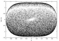
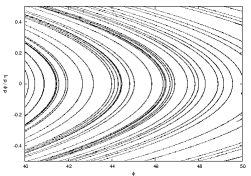
Figure 3: The Poincaré section for the model class I, $a=\phi$ and $a^{\prime}>0$ (upper); $a=0$, $a^{\prime}>0$ (bottom). Motion in narrow field between two hyperbolas is completely regular. Complexity of behavior comes from motion near the origin of the configuration space.

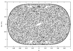
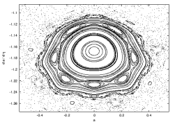
Figure 4: The Poincaré section for the model class II, $\phi=0$ and $\phi^{\prime}>0$. The empty region at the upper section comes from motion of a particle-universe along the $\phi$ ($a=0$) axis.

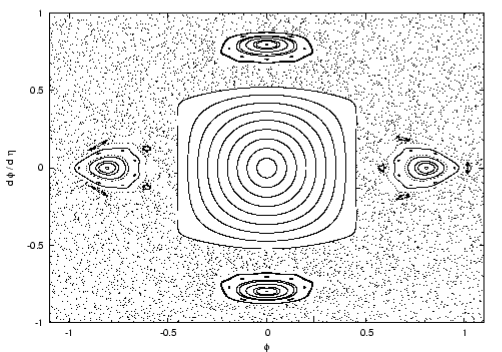
Figure 5: The Poincaré section for the model class II, $a=0$ and $a^{\prime}>0$.

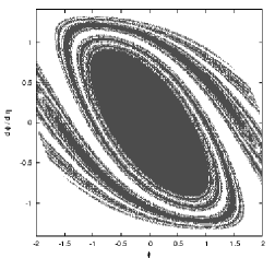
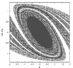
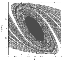
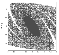
Figure 6: The fractal structure of the phase space of initial conditions of trajectories chosen at $a=0$ and $a^{\prime}>0$ for class I and landing at $|a_{f}|=2$, $3$, $4$, $5$ (grey) or at $|\phi_{f}|=2$, $3$, $4$, $5$ (white), respectively. Complexity of the fractal structure increases with the final state of the trajectories which means that trajectories spend more time in the region near the point $(0,0)$ in the configuration space. The solid areas in the center of figures come from the motion along the $\phi$-axis.

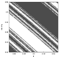
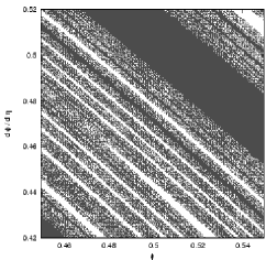
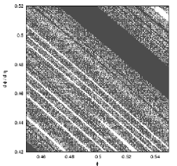
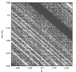
Figure 7: Magnification of the fractal structure of the phase space of initial conditions from Fig. 6.

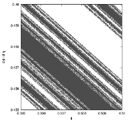
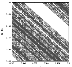
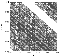
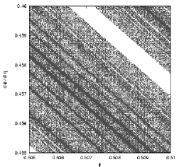
Figure 8: Magnification of the fractal structure of the phase space of initial conditions from Fig. 7.

The idea of the description of a dark energy field in terms of a Higgs field which creates inertial mass through the spontaneously symmetry breaking has been investigated lately Nemiroff and Patla (2004). For $m^{2}<0$ we can distinguish two subclasses of the model with the spontaneously symmetry breaking for which chaotic behavior can be detected

class I: $$\qquad A =B=C=D=0,\quad E>0\mbox{ (or }m^{2}<0),$$

class II: $$\qquad A =B=D=0,\quad C>0\mbox{ (or }\Lambda<0),\quad E>0\mbox{ (or }m^{2}<0).$$

These are flat models with conformally coupled phantom fields for which trajectories have the property of topological transitivity in contrast to the case $m^{2}>0$. In Fig. 1 and 2 we present sample trajectories for both models and evolution for every trajectory is last for the same interval of time. From this simple picture we can initially conclude that the systems are sensitive on initial conditions.

The first class of models is isomorphic with the well known Yang-Mills systems with the potential function $V\propto x^{2}y^{2}$. Because the domain admissible for motion is bounded and its boundary has negative curvature, the property of recurrence of trajectories is present. We consider the both classes of systems on some distinguished energy level $\mathcal{H}=\mathcal{E}\propto\rho_{\rm{r},0}>0$. The Poincaré sections for both classes are represented in Figs. 3, 4, 5. In Fig. 3 it is shown the Poincarè section for the flat cosmological model with vanishing $\Lambda$, $\lambda$, and $m^{2}<0$ (class I). If we postulate additionally the existence of radiation matter in the model than we deal with the system on the constant non-zero energy level. In this case we obtain some chaotic distribution of points on the Poincarè section $(a,\phi^{\prime})$. In Fig. 4 and  5 it is presented the flat cosmological model with the negative cosmological constant $\Lambda$ and $m^{2}<0$ (class II) on the plane $(a,a^{\prime})$. In this case we can observe islands of stability. However, the trajectories wander to the non-physical region of $a<0$. This allows many cycles to be considered if we continue the scale factor into negative values. But what it means physically is not clear.

All these figures illustrate what we proved earlier, namely the standard chaos with recurrence of orbits and the property of sensitive dependence on initial conditions.

We cannot perform the analogous analysis for the class of models with $m^{2}>0$ because there is no chaos in Wiggins’ standard sense. However they possess the property of complex behavior of trajectories similar to the non-chaotic scattering process. Note that the evidence of chaos in terms of fractal basins, Cantori or stochastic layers requires the recurrence of trajectories. Similarly the Poincaré sections can be constructed from many cycles for a useful picture to emerge Cornish and Levin (1996).

In the case of $m^{2}<0$, trajectories of the system return to the neighborhood of the origin time after time and we have the multiple scattering process on the potential walls (boundaries of the domain admissible for motion). We can control and count how many times the trajectory gets closer to the origin than some fixed distance from the origin. With increasing this fix distance the number of controlled scattering events increases and a more complicated fractal structure arises. Fig. 6, 7 and 8 illustrate fractal structures of the phase space of initial conditions for trajectories reaching some values $a_{f}$ and $\phi_{f}$ at some moment of time evolution. The fractal dimension calculated by counting cells which contain light and dark areas (i.e. leading to two types of the final outcome) is $a_{f}=\phi_{f}=2$ — $D_{0}=1.676$; $a_{f}=\phi_{f}=3$ — $D_{0}=1.888$; $a_{f}=\phi_{f}=4$ — $D_{0}=1.953$; $a_{f}=\phi_{f}=5$ — $D_{0}=1.971$. The chosen method of counting cell enables us to order fractals with respect to the increasing complexity, i.e. for a nearly regular system the fractal dimension is close to one, in turn for a completely chaotic one is approaching two. One can also observe that complexity of dynamical behavior of trajectories grows more the longer trajectories come more often in the neighborhood of the origin of the coordinate system because the motion between branches of hyperbolas is regular (see Fig. 3).

Fig. 9, 10, 11 and 12 present the fractal structure of phase space of initial conditions for the category II model. At enough small value of $\phi_{f}$ the system is regular and no chaotic behavior is present (Fig. 9). With an increasing value of $\phi_{f}$: $\phi_{f}=2$ — $D_{0}=1.812$; $\phi_{f}=3$ — $D_{0}=1.967$, we observe the transition to chaos which cause to emerge the fractal structure of the space of initial conditions (Fig. 10–12).

In Fig. 13 we plot the phase space of initial conditions chosen at $a=0$ and $a^{\prime}>0$ calculated from the Hamiltonian which lead to a given property in one cycle of evolution, i.e. to maximal expansion with a positive value of $\phi$ (grey) or negative value of $\phi$ (white) – left image, and back to a final singularity again with a positive value of $\phi$ (grey) or a negative value of $\phi$ (white) – right image. Therefore if we consider evolution in a physical domain between initial and final singularities this system cannot be chaotic. If we prolong its evolution to the non-physical domain $a<0$ then we obtain chaos. Note that non-integrability indicators measure the true intrinsic complexity of the system in both cases Szydlowski et al. (2005).

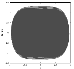
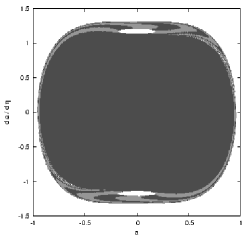
Figure 9: The structure of phase space of initial conditions for class II trajectories chosen at $\phi=0$ and $\phi^{\prime}>0$ and landing at $\phi=0.75$ (dark grey) and $\phi=-0.75$ (grey) presented in left figure and $\phi=0.9$ (dark grey) and $\phi=-0.9$ (grey) in right figure. The white poles correspond to the centers of stability in Fig. 4.

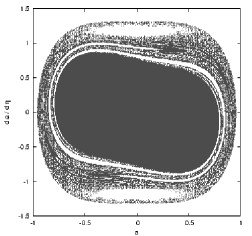
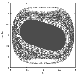
Figure 10: The fractal structure of phase space of initial conditions of trajectories class II landing at $\phi=2$ (left) and $\phi=3$ (right). Initial conditions leading to negative values of $\phi$ omitted for clarity.

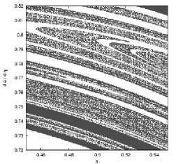
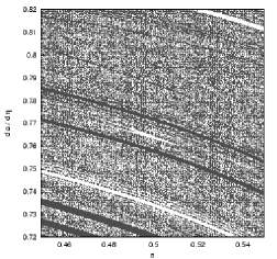
Figure 11: Magnification of the fractal structure of the phase space of initial conditions of trajectories class II from Fig. 10.

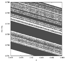
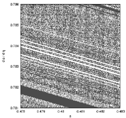
Figure 12: Magnification of the fractal structure of the phase space of initial conditions of trajectories class II from Fig. 11.

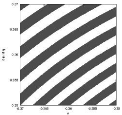
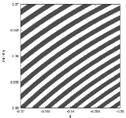
Figure 13: The structure of phase space of initial conditions for model class I chosen at $a=0$ with $a^{\prime}>0$ for trajectories leading to $a^{\prime}=0$ (or equivalent $H=0$) with $\phi>0$ (grey) and $\phi<0$ (white) – the left image, and initial conditions of trajectories leading to $a=0$ with $\phi>0$ (grey) and $\phi<0$ (white) – the right image. There is no chaos in one cycle of evolution.

IV Phantom cosmology as the scattering process

In this section we investigate behavior of a model without the spontaneously symmetry breaking. This is a model with $A=B=C=D=0$ and $E=-1$ ($m^{2}=2$) on different energy levels $\mathcal{E}>0$, $\mathcal{E}=0$ and $\mathcal{E}<0$.

In the analysis of this case we explore analogy to the classical system in which appears the chaotic scattering. From the equation of motion we obtain that for any initial condition trajectories escape to infinity ($\phi\to\pm\infty$ $a\to\pm\infty$ as time goes to infinity). For energy $\mathcal{E}>0$ the configuration space is unbounded and trajectories pass from one quadrant to another. On the other hand for $\mathcal{E}\leq 0$ motion is restricted to only this quadrant of the configuration space where the initial conditions are.

In Fig. 14 we present the analysis of dependence of scattering on the energy level. For this aim the initial condition in the configuration space are chosen on the line $\phi=-a+10$ with $a^{\prime}=\phi^{\prime}<0$ under the conservation of the Hamiltonian constraint. For $\mathcal{E}\leq 0$ trajectories go toward the origin of coordinate system and after some time escape to infinity passing through a line $\phi=-a+10$. On the $x$-axis we mark the initial value of $a$ and $y$-axis we mark final distance from the symmetry point with coordinates $(5,5)$ at the moment of intersection of line of initial conditions. In this figure there is no discontinuities, we do not also observe the fluctuation of distance $d_{f}$. It enable us to conclude that we deal with the scattering process although the domain of interaction is not finite Ott (1993). So there is no chaotic scattering. The motion of the system is regular and there is no sensitivity of motion with respect to initial conditions.

For a deeper confirmation of this statement we study numerically a larger number of initial conditions (Fig. 15). In the configuration space the initial conditions are chosen as previously, i.e. $\phi=-a+10$ and the initial conditions for velocities are parameterized in a natural way by an angle $\alpha$, i.e. $a^{\prime}=-V(a,\phi,\mathcal{E})\cos\alpha$, $\phi^{\prime}=-V(a,\phi,\mathcal{E})\sin\alpha$ where $V(a,\phi,\mathcal{E})=\sqrt{\mathcal{E}+m^{2}a^{2}\phi^{2}}$. In Fig. 15 (a) and (b) it is presented results of our analysis for $\mathcal{E}<0$ and $\mathcal{E}=0$ respectively. The grey area corresponds to initial conditions for which trajectories pass through line $\phi=-a+10$ with $\phi>a$. Fig. 15 (c) illustrates domains of initial conditions for $\mathcal{E}>0$ for which trajectories outcomes reach different quadrants : I quadrant – dark grey, II quadrant – grey, III quadrant – black, IV quadrant — medium grey. The black line presents initial conditions taken from Fig. 14. We cannot observe chaotic scattering in this case.

Figure 14: The scattering process in the class A model without the spontaneously symmetry breaking. For all trajectories initial conditions were chosen at line $\phi=-a+10$ in configuration space and $\dot{a}=\dot{\phi}<0$ calculated from the Hamiltonian. On the $x$-axis we put initial position $a$ and on the $y$-axis we put a final distance from a symmetry point in the configuration space $(5,5)$ when a trajectory is escaping to infinity. For $\mathcal{E}<0$ (a) and $\mathcal{E}=0$ (b) all the trajectories escape to infinity ($a\to\infty,\phi\to\infty$) without crossing $a=0$ or $\phi=0$. For $\mathcal{E}>0$ (c) some trajectories change a quarter after starting from I quarter: I – solid line, II – dashed line, III – dotted line and IV – dash-dot line.

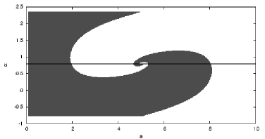
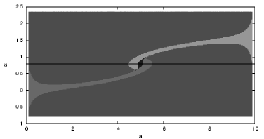
Figure 15: The scattering process in the class A model without the spontaneously symmetry breaking for a large number of trajectories. (See text for description). Fig. (a) and (b) correspond to $\mathcal{E}<0$ and $\mathcal{E}=0$, respectively. The grey areas correspond to initial conditions for which trajectories pass through the line $\phi=-a+10$ with $\phi>a$. Fig. (c) corresponds $\mathcal{E}>0$ (the configuration space is unbounded) and illustrates domains of initial conditions for which trajectories outcomes reach different quadrants: I quadrant – dark grey, II quadrant – grey, III quadrant – black, IV quadrant — medium grey. The black lines represent initial conditions from Fig. 14.

V Acceleration in Phantom Cosmology

The current Universe is in an accelerating phase of expansion that’s why we check whether the scalar fields in the FRW cosmology can explain this phenomenon. For this aim let’s are consider acceleration equation which can be obtained from the Raychaudhury equation

$$\frac{\ddot{a}}{a}=-(\rho+3p)=-(-2\dot{\psi}^{2}-2U(\psi)+3\xi H(\psi^{2})\dot{}+3\xi(\psi^{2})\ddot{}+6\xi\dot{H}\psi^{2}+6\xi H^{2}\psi^{2})-2\rho_{r}$$ (24)

In the special case of the phantom field minimally coupled to gravity $\xi=0$ and without radiation $\rho_{r}=0$ we have

$$\frac{\ddot{a}}{a}=2(\dot{\psi}^{2}+U(\psi)).$$ (25)

Next, for zero energy level and $\Lambda=0$ from (13) we have that

$$H^{2}=2\rho_{\psi}=-\dot{\psi}^{2}+2U(\psi).$$ (26)

and finally we receive the acceleration equation which independent of the form of the potential function

$$\frac{\ddot{a}}{a}=3\dot{\psi}^{2}+H^{2}\geq 0.$$ (27)

In the case of conformally coupled phantom field $\xi=1/6$ we have

$$\frac{\ddot{a}}{a}=-(-\dot{\psi}^{2}-2U(\psi)-H^{2}\psi^{2}-H(\psi^{2})\dot{}+\psi\frac{\mathop{\rm{d}}U}{\mathop{\rm{d}}\psi}(\psi))-2\rho_{r}$$ (28)

and after the rescaling time and field variables: $\mathop{\rm{d}}t=a\mathop{\rm{d}}\eta$, $\phi=a\psi$ and inserting the potential function (5) we have

$$\frac{\ddot{a}}{a}=\frac{1}{a^{4}}(\phi^{\prime 2}-\frac{1}{2}\lambda\phi^{4}-2\rho_{r,0}),$$ (29)

where prime denotes differentiation with respect to the conformal time and dot with respect to the cosmological time. We can also express equation of state parameter (8) in these new variables

$$w_{\phi}\equiv\frac{p_{\phi}}{\rho_{\phi}}=\frac{\frac{1}{a^{4}}(-\frac{1}{6}\phi^{\prime 2}-\frac{1}{6}m^{2}a^{2}\phi^{2}+\frac{1}{12}\lambda\phi^{4})}{\frac{1}{a^{4}}(-\frac{1}{2}\phi^{\prime 2}+\frac{1}{2}m^{2}a^{2}\phi^{2}+\frac{1}{4}\lambda\phi^{4})}.$$ (30)

We clearly see that this is a good expression only if $a\neq 0$. For the physical region $a>0$ we can express the effective equation of state parameter as

$$w_{\rm{eff}}\equiv\frac{-\frac{1}{6}\phi^{\prime 2}-\frac{1}{6}m^{2}a^{2}\phi^{2}+\frac{1}{3}\rho_{r,0}}{-\frac{1}{2}\phi^{\prime 2}+\frac{1}{2}m^{2}a^{2}\phi^{2}+\rho_{r,0}}$$ (31)

In Fig. 16 we show the evolution of acceleration and evolution of coefficient of the equation of state $w_{\phi}$ for model class I (flat model with $m^{2}<0$) with respect to the conformal time $\eta$ which is monotonous function of the cosmological time in the physical domain. Note that in the case of $m^{2}<0$ the universe is decelerating and $w_{\phi}$ stays in the interval $\langle-1/3;1/3\rangle$, with $w_{\phi}=-1/3$ when $\phi^{\prime}=0$ and $w_{\phi}=1/3$ when $\phi=0$.

The analogous analysis made for the model class A without the spontaneously symmetry breaking (presented in Fig. 17) shows that the universe is always accelerating. In this case pressure $p_{\phi}$ is always negative. In the case of $\mathcal{E}>0$ we can have positive value of $w_{\phi}$ and this means that density can be negative. Moreover, during evolution there are crossings of the line $w_{\phi}=-1$ and then $w_{\rm{eff}}$ goes to minus one. The amplitude of these oscillations depends on $\rho_{\rm{r},0}$.

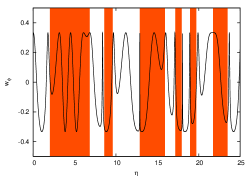
Figure 16: The evolution of acceleration from Eq. (29) with $\lambda=0$ (left panel) and equation of state parameter $w_{\phi}$ from Eq. (30) (right panel) for model class I with respect to conformal time for short period of time for trajectory from left panel of Fig. 1. Shaded area denote unphysical regions of scale factor $a\leq 0$. In physical regions acceleration is always negative $\ddot{a}\leq 0$ model decelerates and equation of state parameter never crosses $w_{\phi}=-1$ barrier.

Figure 17: The evolution of acceleration from Eq. (29) (left panel) and the equation of the state parameter $w_{\rm{eff}}$ from Eq. (31) (right panel) for model class A without spontaneously symmetry breaking for a sample trajectory starting from the same initial conditions in the configuration space ($a_{0}=4.75$, $\phi_{0}=-a_{0}+10$ and $a_{0}^{\prime}=\phi_{0}^{\prime}<0$ calculated from the Hamiltonian constrain) but for different energy levels: $\mathcal{E}<0$ (top), $\mathcal{E}=0$ (middle) and $\mathcal{E}>0$ (bottom). For every sample we have acceleration but the equation of the state parameter oscillates and aproaches $w_{\rm{eff}}=-1$.

VI Conclusions

In cosmology the Mixmaster models are well known for their chaotic behavior Cornish and Levin (1996). In these models chaos is caused by anisotropy of space. In this paper we considered the phantom cosmological models which are homogeneous and isotropic where the chaos is the consequence of the nonlinearity of the potential function for the scalar field. We found chaos is a generic feature of the phantom cosmology with the spontaneously symmetry breaking. It assumes the form of the multiple chaotic scattering process. In the case of the absence of symmetry breaking we did not find the sensitivity over initial conditions and the system behaves as the standard scattering process.

There is no difference between the flat universes filled with minimal and conformally coupled scalar fields. As it was demonstrated by Faraoni et al. Gunzig et al. (2000); Faraoni et al. (2006) there is no chaos for the former class of models because the solution corresponding $k=0$ are restricted to move in some two-dimensional submanifold of the phase space $(H,\phi,\dot{\phi})$. There are no enough room for chaotic motion manifestation. The analogous result is valid for the other value of the coupling constant $\xi$. Note that we can observe chaotic behavior in some cases of the conformally coupled scalar field in the flat universes, when we consider the system on non-zero energy level. Physically it means that the universe is filled with radiation matter.

The reason for which the flat universes with scalar field are non-chaotic lies in lack of invariant measure of chaotic behavior in the general relativity Szydlowski and Krawiec (1996); Motter (2003). In general the standard chaos indicators like Lyapunov exponents or Kolmogorov-Sinai entropy depends on time parameterization. In general relativity there is freedom of choice of the lapse function which defines reparameterization of time. The Hamiltonian is given modulo the lapse function. Therefore if we consider the Hamiltonian FRW system with scalar field on zero energy level it is possible that in the Hamiltonian constraint $a$ i $\dot{a}$ appear only in the combination $H=\dot{a}/a$. Hence the motion of the system takes place in the 3-dimensional phase space $h(H,\phi,\dot{\phi})=0$ on some 2-dimensional submanifold. For any value of coupling constant and general class of potentials there is no place for chaos (even the models with the cosmological constant).

The new picture appears if the system is described on a non-zero energy level. Then the motion of the system is in the 3-dimensional submanifold of the 4-dimensional phase space. But in general case there is no possibility of choosing the lapse function in such a way that $a$ i $\dot{a}$ contribute in the Hamiltonian constraint by the Hubble function.

Among the conformally coupled models there are in principal two types of behavior. First, chaotic scattering process takes place for case $m^{2}<0$ (the spontaneously symmetry breaking). In this case trajectories possess the property of topological transitivity which guarantees their recurrence in the phase space and the scattering process takes place around the origin. It is similar to the chaos appeared in the Yang-Mills theory. Exploring this analogy to this system we calculate a Gaussian curvature of the potential function which measure local instability of nearby trajectories. We proof that this curvature is negative. Because the configuration space is bounded in this case the mixing of trajectories is observed.

Second, in the opposite case of $m^{2}>0$ we characterize dynamics in the system in terms of symbolic dynamics. No fractal structure in the space of initial conditions was found and conclude that the scattering process has not the chaotic character.

We also found that the universe filled with conformally coupled scalar field is accelerating without the positive cosmological constant. In principle, there are two sources of this acceleration. The acceleration is driven by negative energy density and coefficient of equation of state $w_{\phi}$ is greater than $-1/3$. Alternatively, energy density is positive and the coefficient of equation of state can be smaller than $-1/3$. The latter there is crossing of $w_{\phi}=-1$. Of course, for the explanation of SNIa data apart from the acceleration of the Universe itself, the rate of acceleration is also crucial.

The system with phantom scalar field coupled conformally to gravity in the FRW universe can be treated as scattering process with chaotic and nonchaotic character. The generic feature of this class of systems with the spontaneously symmetry breaking is the chaotic scattering of trajectories.