String-inspired cosmology: Late time transition from scaling matter era to dark energy universe caused by a Gauss-Bonnet coupling

Abstract

The Gauss-Bonnet (GB) curvature invariant coupled to a scalar field $\phi$ can lead to an exit from a scaling matter-dominated epoch to a late-time accelerated expansion, which is attractive to alleviate the coincident problem of dark energy. We derive the condition for the existence of cosmological scaling solutions in the presence of the GB coupling for a general scalar-field Lagrangian density $p(\phi,X)$, where $X=-(1/2)(\nabla\phi)^{2}$ is a kinematic term of the scalar field. The GB coupling and the Lagrangian density are restricted to be in the form $f(\phi)\propto e^{\lambda\phi}$ and $p=Xg(Xe^{\lambda\phi})$, respectively, where $\lambda$ is a constant and $g$ is an arbitrary function. We also derive fixed points for such a scaling Lagrangian with a GB coupling $f(\phi)\propto e^{\mu\phi}$ and clarify the conditions under which the scaling matter era is followed by a de-Sitter solution which can appear in the presence of the GB coupling. Among scaling models proposed in the current literature, we find that the models which allow such a cosmological evolution are an ordinary scalar field with an exponential potential and a tachyon field with an inverse square potential, although the latter requires a coupling between dark energy and dark matter.

I Introduction

A great deal of efforts in modern cosmology, over the course of the past decade, have been made in trying to understand the nature and the origin of dark energy which is responsible for late-time acceleration of the universe obser ; review ; CST . Although cosmological constant is the simplest candidate of dark energy consistent with current observations, it suffers from a severe fine-tuning problem from a field theoretic point of view Weinberg . It is then tempting to find alternative models of dark energy which have dynamical nature unlike cosmological constant. An accelerated expansion can be realized by using a scalar field whose origin may be found in superstring or supergravity theories. Thus modern particle physics has been an attractive supplier for the construction of scalar-field dark energy models–such as quintessence quin , K-essence Kes , tachyon tachyon , dilatonic models Gas , and ghost condensate ghostcon ; PT04 .

Although the dynamically evolving field models have an edge over the cosmological constant scenario, they too, in general, involve fine-tuning of initial values of the field and the parameters of the model. Secondly, nucleosynthesis places stringent restriction on any additional degree of freedom (over and above the particle physics standard model degrees of freedom) which translates into a constraint on the ratio of the field energy density to the energy density of the background fluid CST . These problems can be addressed by employing scalar field models exhibiting scaling solutions Fer ; CLW ; scaling ; TS04 ; Tsuji06 ; AQTW . For instance, a standard scalar field $\phi$ with an exponential potential in General Relativity (GR) Fer ; CLW can mimic the background (radiation/matter) remaining sub-dominant so as to respect the nucleosynthesis constraint Nelson . The scaling solutions as dynamical attractors can successfully address the second problem and can also considerably alleviate the fine-tuning problem of initial conditions.

For a viable cosmological evolution, the scalar field should remain unimportant for most of the cosmic evolution and should emerge from the hiding epoch only at late times to give rise to the accelerated expansion. Since scaling solutions are non-accelerating, the model should be supplemented by an additional mechanism allowing the field to exit from the scaling regime at late times. There are several ways of achieving this goal:

• (i) At late times the potential becomes shallow to lead to the accelerated expansion. For example this is realized by the double exponential potential given by $V(\phi)=V_{0}(e^{-\lambda\kappa\phi}+e^{-\mu\kappa\phi})$ with $\lambda^{2}>20$ and $\mu^{2}<2$ Nelson (here $\kappa^{2}=8\pi G$ with $G$ being gravitational constant).

• (ii) A local minimum of the field potential appears at late times. The examples of this type of models are $V(\phi)=V_{0}[\cosh(\lambda\kappa\phi)-1]^{n}$ Sahni and $V(\phi)=V_{0}e^{-\lambda\kappa\phi}[A+(\kappa\phi-B)^{2}]$ Alb . In the former case the acceleration occurs for $n<1/2$ on average, whereas in the latter case the system always approaches a de-Sitter universe after a damped oscillation of the field.

• (iii) Assisted quintessence KLT . This is realized by considering many fields $\phi_{i}$ with the sum of the exponential potential $V=\sum A_{i}e^{-\lambda_{i}\kappa\phi_{i}}$, since the presence of many scalar fields leads to the smaller effective coupling, i.e., $\lambda_{\rm eff}^{-2}=\sum\lambda_{i}^{-2}$ Liddle .

Although these are interesting attempts to provide a successful exit from the scaling regime, it is fair to say that the aforementioned mechanisms are still phenomenological. It is of great importance to find cosmological models from fundamental theories of particle physics like string theory which may incorporate the findings of the phenomenological studies. String theory necessarily includes scalar fields (dilaton $\&$ modulus fields); the low energy string effective action also gives rise to a modification of standard GR in terms of Riemann invariants coupled to scalar field(s) reviewstring . The modifications are important to address the problems of past past and future future singularities. Out of these corrections, the Gauss-Bonnet (GB) term is of a special relevance. The GB term is a topological invariant quantity which contributes to the dynamics in 4 dimensions provided it is coupled to a dynamically evolving scalar field. It is the unique invariant for which the highest (second) derivative occurs linearly in the equations of motion thereby ensuring the uniqueness of solutions. Nojiri et al. NOS studied scalar-Gauss-Bonnet cosmology to demonstrate the existence of a particular dark energy solution. Such a solution exists in the presence of an exponential potential $V(\phi)\propto e^{-\lambda\kappa\phi}$ and the GB coupling $f(\phi)\propto e^{\mu\kappa\phi}$. More recently Koivisto and Mota KM06 showed that the GB coupling allows a possibility to lead to the exit from the scaling matter era to the dark energy dominated universe for the same model. See Refs. CTS ; Neupane ; NO05 ; Cog06 ; Cal ; Sami06 ; Annalen ; Sanyal ; Andrew for other aspects of the GB dark energy scenario.

In this paper we shall clarify the form of the GB coupling $f(\phi)$ for the existence of scaling solutions by starting from a very general scalar-field Lagrangian density $p(\phi,X)$ where $X$ is a kinematic term of the field. This includes a wide variety of scalar-field models such as quintessence, K-essence, tachyon, and ghost condensate. The demand for scaling solutions not only determines the field Lagrangian to be $p(\phi,X)=Xg(Xe^{\lambda\phi})$ ($g$ is an arbitrary function) but also fixes the GB coupling in the form $f(\phi)\propto e^{\lambda\phi}$ (here we use the unit $\kappa^{2}=1$). Thus our results are useful to construct viable dark energy models which possess scaling solutions in the matter-dominated epoch. We then investigate the fixed points for the scaling Lagrangian $p(\phi,X)=Xg(Xe^{\lambda\phi})$ with a GB coupling $f(\phi)\propto e^{\mu\phi}$. We show the existence of a pure de-Sitter fixed point which exists only for specific models and study a possibility to obtain a scaling matter era that finally approaches the de-Sitter solution. A standard field with an exponential potential is a specific model to realize such a cosmological evolution provided that $\mu>\lambda$. A tachyon field also possesses the de-Sitter fixed point, but it does not have a scaling matter epoch. However the scaling matter era followed by the de-Sitter solution is possible if dark energy couples to dark matter. We shall discuss cosmological dynamics in such cases in details.

II The condition for the existence of scaling solutions in Gauss-Bonnet cosmology

The model we study is given by the following action

$$S=\int{\rm{d}}^{4}x\sqrt{-g_{M}}\left[\frac{1}{2\kappa^{2}}R+p(X,\phi)-f(\phi)R_{{\rm GB}}^{2}\right]+S_{m}[\phi,\psi_{i},g_{\mu\nu}],$$ (1)

where $g_{M}$ is a metric determinant, $R$ is a Ricci scalar, $p(\phi,X)$ is a Lagrangian density in terms of a scalar field $\phi$ and a kinematic energy $X=-(1/2)g^{\mu\nu}\partial_{\mu}\phi\>\partial_{\nu}\phi$. The Gauss-Bonnet (GB) term, $R_{{\rm GB}}^{2}\equiv R^{2}-4R_{\mu\nu}R^{\mu\nu}+R_{\alpha\beta\mu\nu}R^{\alpha\beta\mu\nu}$, couples to the field $\phi$ through the coupling $f(\phi)$. We allow for an arbitrary coupling between the matter fields $\psi_{i}$ and the scalar field $\phi$. We assume that the field $\phi$ is coupled to a barotropic perfect fluid (energy density $\rho_{m}$ and pressure density $p_{m}$) with a coupling given by Lucacoupled ; LucaST ; GNST

$$Q=-\frac{1}{\rho_{m}\sqrt{-g_{M}}}\frac{\delta S_{m}}{\delta\phi}\,.$$ (2)

Note that the energy density of the scalar field is given by $\rho=2X(\partial p/\partial X)-p$ with an equation of state $w_{\phi}=p/\rho$. In what follows we shall use the unit $\kappa^{2}=8\pi G=1$.

In the flat Friedmann-Robertson-Walker background with a scale factor $a$, the equations for $\rho$ and $\rho_{m}$ are

$$\dot{\rho}+3H(1+w_{\phi})\rho=-Q\rho_{m}\dot{\phi}-24f^{\prime}(\phi)\dot{\phi}H^{2}(H^{2}+\dot{H})\,,$$ (3)

$$\dot{\rho}_{m}+3H(1+w_{m})\rho_{m}=+Q\rho_{m}\dot{\phi}\,,$$ (4)

where $H\equiv\dot{a}/a$ is a Hubble parameter. A dot and a prime represent derivatives in terms of cosmic time $t$ and the field $\phi$, respectively. The Hubble parameter satisfies the constraint equation:

$$3H^{2}=\rho_{m}+\rho+24f^{\prime}(\phi)\dot{\phi}H^{3}\,.$$ (5)

Then the energy density of the GB term is given by $\rho_{{\rm GB}}=24f^{\prime}(\phi)\dot{\phi}H^{3}$. We define the fractional densities of the field $\phi$, the GB term, and the matter fluid, respectively, as

$$\Omega_{\phi}\equiv\frac{\rho}{3H^{2}}\,,\quad\Omega_{{\rm GB}}\equiv 8f^{\prime}(\phi)\dot{\phi}H\,,\quad\Omega_{m}\equiv\frac{\rho_{m}}{3H^{2}}=1-\Omega_{\phi}-\Omega_{{\rm GB}}\,.$$ (6)

Scaling solutions are characterised by constant values of $\Omega_{\phi}$, $\Omega_{{\rm GB}}$ and $\Omega_{m}$, or equivalently a constant ratio between each energy density. Then this gives the condition:

$$\frac{{\rm d}\ln\rho}{{\rm d}N}=\frac{{\rm d}\ln\rho_{m}}{{\rm d}N}=\frac{{\rm d}\ln\rho_{{\rm GB}}}{{\rm d}N}\equiv-3(1+w_{\rm eff})\,,$$ (7)

where $w_{\rm eff}$ is an effective equation of state related to the Hubble rate via the relation

$$\frac{\dot{H}}{H^{2}}=-\frac{3}{2}(1+w_{\rm eff})\,.$$ (8)

We also note that $w_{\phi}$ and $w_{m}$ are assumed to be constants in the scaling regime. From Eqs. (3) and (4) together with the scaling condition (7), we find

$$Q\frac{{\rm d}\phi}{{\rm d}N}=\frac{3(w_{m}-w_{\phi})\Omega_{\phi}-\Omega_{{\rm GB}}(1+\dot{H}/H^{2})}{\Omega_{\phi}+\Omega_{m}}\,.$$ (9)

Substituting this relation for Eq. (4) and using the relations (7) and (8), we obtain

$$w_{\rm eff}=\frac{2(w_{m}\Omega_{m}+w_{\phi}\Omega_{\phi}-\Omega_{{\rm GB}}/6)}{1+\Omega_{\phi}+\Omega_{m}}\,.$$ (10)

Hence Eq. (9) can be rewritten as

$$Q\frac{{\rm d}\phi}{{\rm d}N}=\frac{1}{\Omega_{\phi}+\Omega_{m}}\left[3(w_{m}-w_{\phi})\Omega_{\phi}+\Omega_{{\rm GB}}\frac{\Omega_{\phi}(1+3w_{\phi})+\Omega_{m}(1+3w_{m})}{1+\Omega_{\phi}+\Omega_{m}}\right]\equiv C\,(={\rm const})\,.$$ (11)

From these equations and the definition of $X$, we find

$$2X=H^{2}\left(\frac{{\rm{d}}\phi}{{{\rm{d}}N}}\right)^{2}\;\;\propto\;\;\frac{\rho}{{Q^{2}}}\;\;\propto\;\;\frac{p(X,\phi)}{Q^{2}}\,,$$ (12)

which gives

$$\frac{{\rm{d}}\ln X}{{\textrm{d}}N}=-3(1+w_{\rm eff})-2\frac{{\rm{d}}\ln Q}{{\rm{d}}N}\,.$$ (13)

From Eq. (7) together with $p\propto\rho$, the Lagrangian density $p=p(\phi,X)$ satisfies the differential equation

$$\frac{\partial\ln p}{\partial X}\frac{{\rm d}X}{{\rm d}N}+\frac{\partial\ln p}{\partial\phi}\frac{{\rm d}\phi}{{\rm d}N}=-3(1+w_{\rm eff})\,.$$ (14)

Substituting Eqs. (11) and (13) for Eq. (14), we arrive at

$$\left[1+\frac{2}{\lambda Q}\frac{{\rm d}Q(\phi)}{{\rm d}\phi}\right]\frac{\partial\ln p}{\partial\ln X}-\frac{1}{\lambda}\frac{\partial\ln p}{\partial\phi}=1\,,$$ (15)

where

$$\lambda(\phi)\equiv\frac{3(1+w_{\rm eff})}{C}Q(\phi)=\frac{2(1-\Omega_{{\rm GB}})[3(1+w_{m}\Omega_{m}+w_{\phi}\Omega_{\phi})-2\Omega_{{\rm GB}}]}{3(w_{m}-w_{\phi})\Omega_{\phi}(2-\Omega_{{\rm GB}})+\Omega_{{\rm GB}}[1-\Omega_{{\rm GB}}+3(w_{m}\Omega_{m}+w_{\phi}\Omega_{\phi})]}Q(\phi)\,.$$ (16)

Equation (15) is the same form of equation which was obtained in the absence of the GB coupling AQTW . Following the procedure in Ref. AQTW , Eq. (15) restricts the form of the Lagrangian density to be

$$p=XQ^{2}(\phi)g\left[XQ^{2}(\phi)\exp\left(\int^{\phi}\lambda(\varphi){\rm d}\varphi\right)\right]\,,$$ (17)

where $g$ is an arbitrary function. If $Q$ is a constant, this reduces to a simple form:

$$p=Xg(Y)\,,\quad Y\equiv Xe^{\lambda\phi}\,,$$ (18)

where $p$ is redefined so that a constant factor is removed from Eq. (17). This form of the scaling Lagrangian was first derived in Ref. PT04 in the absence of the GB coupling (see also Ref. TS04 for the extension of the analysis to the case $H^{2}\propto\rho^{n}$). Even if the GB term is present, we have shown that the Lagrangian takes the same form with a modified value of $\lambda$ given in Eq. (16). For a later convenience we present several models which belong to the scaling Lagrangian (18).

• (i) An ordinary field with an exponential potential, i.e., $p=X-ce^{-\lambda\phi}$ CLW . This corresponds to the choice

  $$g(Y)=1-c/Y\,.$$ (19)

• (ii) A dilatonic ghost condensate model, i.e., $p=-X+ce^{\lambda\phi}X^{2}$ PT04 . This corresponds to the choice

  $$g(Y)=-1+cY\,.$$ (20)

• (iii) A tachyon field, i.e., $p=-V(\varphi)\sqrt{1-\dot{\varphi}^{2}}$ with $V(\varphi)\propto\varphi^{-2}$ Abramo ; Ruth ; CGST . This corresponds to the choice

  $$g(Y)=-(c/Y)\sqrt{1-2Y}\,.$$ (21)

  Note that the field $\varphi$ is related to $\phi$ via the relation $\varphi=(2/\lambda)e^{\lambda\phi}/2$.

From Eq. (11) we find $\dot{\phi}/H=C/Q$. Since the GB energy density, $\rho_{{\rm GB}}=24f^{\prime}(\phi)\dot{\phi}H^{3}$, satisfies the relation ${\rm d}\ln\rho_{{\rm GB}}/{\rm d}N=-3(1+w_{\rm eff})$ for scaling solutions, one gets

$$\frac{f^{\prime\prime}(\phi)}{f^{\prime}(\phi)}\frac{\dot{\phi}}{H}=3(1+w_{\rm eff})\,.$$ (22)

This yields $f^{\prime\prime}(\phi)/f^{\prime}(\phi)=3(1+w_{\rm eff})Q/C=\lambda$, which gives

$$f^{\prime}(\phi)=\alpha e^{\lambda\phi}\,,$$ (23)

where $\alpha$ is an integration constant. This means that the GB coupling is restricted to be in the form $f(\phi)\propto e^{\lambda\phi}$ for the existence of scaling solutions.

In the case of a non-relativistic dark matter ($w_{m}=0$), the quantity $C$ is given by

$$C=\frac{1-\Omega_{\phi}-\Omega_{m}-6w_{\phi}\Omega_{\phi}}{1+\Omega_{\phi}+\Omega_{m}}\,,$$ (24)

whereas the effective equation of state is

$$w_{\rm eff}=-\frac{1-\Omega_{\phi}-\Omega_{m}-6w_{\phi}\Omega_{\phi}}{3(1+\Omega_{\phi}+\Omega_{m})}\,.$$ (25)

Hence one has a simple relation $w_{\rm eff}=-C/3$. From Eq. (16) we get $C=3Q/(Q+\lambda)$. Then from Eq. (11) we find the following relation along the scaling solution:

$$\frac{\dot{\phi}}{H}=\frac{3}{Q+\lambda}\,.$$ (26)

This is the same relation as in the case where the GB term is absent PT04 ; TS04 .

III Autonomous equations and fixed points

In this section we shall obtain fixed points for the scaling Lagrangian (18). We take into account the contribution of both non-relativistic dark matter ($w_{m}=0$) and radiation ($w_{r}=1/3$), in which case the Friedmann equation is

$$3H^{2}=\rho_{m}+\rho_{r}+\rho+24f^{\prime}(\phi)\dot{\phi}H^{3}\,.$$ (27)

Here the energy density of the scalar field is given by $\rho=X(g+g_{1})$, where $g_{n}\equiv Y^{n}g^{(n)}(Y)$ with $g^{(n)}(Y)$ being the $n$-th derivative in terms of $Y$. We assume that the field $\phi$ is coupled to dark matter with a coupling $Q$ and that it is uncoupled to radiation, as it is the case in the context of scalar-tensor theories LucaST . Hence the equations for the energy densities of dark matter and radiation are

$$\dot{\rho}_{m}+3H\rho_{m}=+Q\rho_{m}\dot{\phi}\,,$$ (28)

$$\dot{\rho}_{r}+4H\rho_{r}=0\,.$$ (29)

The scalar-field equation (3) can be written as

$$\ddot{\phi}+3AH(g+g_{1})\dot{\phi}+\lambda X\left[1-A(g+2g_{1})\right]+24f^{\prime}(\phi)AH^{2}(H^{2}+\dot{H})+AQ\rho_{m}=0\,,$$ (30)

where $A$ is defined by

$$A\equiv(g+5g_{1}+2g_{2})^{-1}\,.$$ (31)

We shall define the following dimensionless quantities:

$$x_{1}\equiv\frac{\dot{\phi}}{\sqrt{6}H}\,,\quad x_{2}\equiv\frac{e^{-\lambda\phi/2}}{\sqrt{3}H}\,,\quad x_{3}\equiv f^{\prime}(\phi)H^{2}\,,\quad x_{4}\equiv\frac{\sqrt{\rho_{r}}}{\sqrt{3}H}\,.$$ (32)

Then the energy fractions are

$$\Omega_{\phi}=x_{1}^{2}(g+2g_{1})\,,\quad\Omega_{{\rm GB}}=8\sqrt{6}x_{1}x_{3}\,,\quad\Omega_{r}=x_{4}^{2}\,,\quad\Omega_{m}=1-\Omega_{\phi}-\Omega_{{\rm GB}}-\Omega_{r}\,.$$ (33)

The variable $Y$ defined in Eq. (18) can be expressed as

$$Y=x_{1}^{2}/x_{2}^{2}\,.$$ (34)

The GB coupling $f^{\prime}(\phi)$ takes the form (23) for the existence of scaling solutions. We shall derive autonomous equations for a more general case:

$$f^{\prime}(\phi)=\alpha e^{\mu\phi}\,.$$ (35)

Since $\mu=\lambda$ for scaling solutions, one has the relation

$$x_{2}^{2}x_{3}=\alpha/3\,.$$ (36)

In this case the variable $x_{3}$ is not needed to study a dynamical system.

Taking the time-derivative of Eq. (27) with the use of Eqs. (28) and (29), we obtain

$$2\dot{H}=-2X(g+g_{1})-\rho_{m}-\frac{4}{3}\rho_{r}+8\left[f^{\prime\prime}(\phi)\dot{\phi}^{2}H^{2}+f^{\prime}(\phi)H(\ddot{\phi}H+2\dot{\phi}\dot{H}-\dot{\phi}H^{2})\right]\,.$$ (37)

Eliminating the $\ddot{\phi}$ term from Eqs. (30) and (37), one gets the following relation

$$(1-8\sqrt{6}x_{1}x_{3}+96Ax_{3}^{2})\frac{\dot{H}}{H^{2}} = -\frac{1}{2}(3+3gx_{1}^{2}+x_{4}^{2})$$ (38)

$$+4x_{3}\biggl{[}2\sqrt{6}x_{1}+3(2\mu-\lambda)x_{1}^{2}+3A\biggl{\{}-\sqrt{6}(g+g_{1})x_{1}+(Q+\lambda)x_{1}^{2}(g+2g_{1})$$

$$-8x_{3}+Q(x_{4}^{2}-1)+8\sqrt{6}Qx_{1}x_{3}\biggr{\}}\biggr{]}\,.$$

The autonomous equations are

$$\frac{{\rm d}x_{1}}{{\rm d}N} = -3A(g+g_{1})x_{1}+\frac{\sqrt{6}}{2}\left[A(Q+\lambda)(g+2g_{1})x_{1}^{2}-\lambda x_{1}^{2}+QA(x_{4}^{2}-1+8\sqrt{6}x_{1}x_{3})\right]$$ (39)

$$-4\sqrt{6}Ax_{3}-(x_{1}+4\sqrt{6}Ax_{3})\frac{\dot{H}}{H^{2}}\,,$$

$$\frac{{\rm d}x_{2}}{{\rm d}N} = -x_{2}\left(\frac{\sqrt{6}}{2}\lambda x_{1}+\frac{\dot{H}}{H^{2}}\right)\,,$$ (40)

$$\frac{{\rm d}x_{3}}{{\rm d}N} = 2x_{3}\left(\frac{\sqrt{6}}{2}\mu x_{1}+\frac{\dot{H}}{H^{2}}\right)\,,$$ (41)

$$\frac{{\rm d}x_{4}}{{\rm d}N} = -x_{4}\left(2+\frac{\dot{H}}{H^{2}}\right)\,,$$ (42)

where $\dot{H}/H^{2}$ is given in Eq. (38).

In what follows we will obtain fixed points in the absence of radiation ($x_{4}=0$). Let us consider the cases: (i) $\lambda=\mu$ and (ii) $\lambda\neq\mu$ separately. We shall study the case $\lambda>0$ without loss of generality.

III.1 Case of $\lambda=\mu$

As we showed in the previous section, there exist scaling solutions for $\lambda=\mu$. Taking note of the relation (36), neither $x_{2}$ nor $x_{3}$ is identical to zero if $\alpha\neq 0$. When $\alpha$ is negligibly small, $x_{2}$ and $x_{3}$ can be very small as well. In this case we may regard $x_{2}\approx 0$ or $x_{3}\approx 0$ as approximate fixed points in Eqs. (40) and (41). Here we do not consider such fixed points, but in the next subsection we will discuss those cases when $\lambda$ does not equal to $\mu$.

Then from Eqs. (40) and (41), the critical points corresponding to $x_{2}\neq 0$ and $x_{3}\neq 0$ satisfy

$$\frac{\dot{H}}{H^{2}}=-\frac{\sqrt{6}}{2}\lambda x_{1}\,.$$ (43)

Then substituting Eq. (43) for Eq. (39), we get

$$(Q+\lambda)(g+2g_{1})x_{1}^{2}-Q-\sqrt{6}(g+g_{1})x_{1}+4x_{3}\left[\sqrt{6}(2Q+\lambda)x_{1}-2\right]=0\,.$$ (44)

From Eqs. (38) and (43), we find

$$3gx_{1}^{2}-\sqrt{6}\lambda x_{1}+3=8x_{1}x_{3}(2\sqrt{6}-3\lambda x_{1})\,.$$ (45)

We note that the following useful relations hold for the scaling Lagrangian (18):

$$w_{\phi}=\frac{g}{g+2g_{1}}\,,\quad w_{\phi}\Omega_{\phi}=gx^{2}\,,\quad g+g_{1}=\frac{(1+w_{\phi})\Omega_{\phi}}{2x^{2}}\,.$$ (46)

Substituting these expressions for Eqs. (44) and (45) and eliminating the $w_{\phi}\Omega_{\phi}$ term, we obtain

$$\left[2(Q+\lambda)x_{1}-\sqrt{6}\right](1-\Omega_{\phi}-\Omega_{{\rm GB}})=0\,.$$ (47)

This gives the following fixed points:

• (a) Scaling solution: $x_{1}=\frac{\sqrt{6}}{2(Q+\lambda)}$ ,

• (b) Scalar-field $\&$ GB dominated point: $\Omega_{\phi}+\Omega_{{\rm GB}}=1$ .

Since both points satisfy the relation (43), the effective equation of state is

$$w_{\rm eff}=-1+\frac{\sqrt{6}}{3}\lambda x_{1}\,.$$ (48)

In what follows we shall discuss two fixed points separately.

III.1.1 Scaling solutions

First we recall that Eq. (26) also gives $x_{1}=\frac{\sqrt{6}}{2(Q+\lambda)}$. From Eq. (48) the effective equation of state is given by

$$w_{\rm eff}=-\frac{Q}{Q+\lambda}\,,$$ (49)

which is independent of the form of $p(\phi,X)$. The accelerated expansion occurs for $w_{\rm eff}<-1/3$, i.e., $Q>\lambda/2$ or $Q<-\lambda$.

From Eq. (45) we get

$$x_{3}=\frac{2Q(Q+\lambda)+3g(Y)}{8(4Q+\lambda)}\,,$$ (50)

where

$$Y=\frac{x_{1}^{2}}{x_{2}^{2}}=\frac{9}{2(Q+\lambda)^{2}\alpha}x_{3}\,.$$ (51)

Once the form of $g(Y)$ is specified, one gets $x_{3}$ and $Y$ from Eqs. (50) and (51). This then determines

$$\Omega_{\phi}=\frac{3}{2(Q+\lambda)^{2}}(g+2g_{1})\,,\quad\Omega_{{\rm GB}}=\frac{24}{Q+\lambda}x_{3}\,.$$ (52)

Let us consider an ordinary scalar field with an exponential potential, i.e., the model given in Eq. (19). In this case we get

$$x_{3}=\frac{6Q(Q+\lambda)+9-\sqrt{[6Q(Q+\lambda)+9]^{2}-192c\alpha(4Q+\lambda)(Q+\lambda)^{2}}}{48(4Q+\lambda)}\,.$$ (53)

We have chosen a minus sign in Eq. (53) to recover $x_{3}\to 0$ as $\alpha\to 0$. When $Q=0$ this reduces

$$x_{3}=\frac{3}{16\lambda}\left[1-\sqrt{1-\frac{64}{27}c\alpha\lambda^{3}}\right]\,,$$ (54)

and also we obtain

$$\Omega_{\phi}=\frac{3}{2\lambda^{2}}\left[1+\frac{32c\alpha\lambda^{3}}{27(1-\sqrt{1-64c\alpha\lambda^{3}/27})}\right]\,,\quad\Omega_{{\rm GB}}=\frac{9}{2\lambda^{2}}\left[1-\sqrt{1-\frac{64}{27}c\alpha\lambda^{3}}\right]\,.$$ (55)

If $c\alpha\lambda^{3}$ is much smaller than unity, we find the following approximate fixed points:

$$x_{2}\simeq\sqrt{\frac{3}{2c\lambda^{2}}}\,,\quad x_{3}\simeq\frac{2}{9}c\alpha\lambda^{2}\,,$$ (56)

together with

$$\Omega_{\phi}\simeq\frac{3}{\lambda^{2}}\left(1-\frac{8}{27}c\alpha\lambda^{3}\right)\,,\quad\Omega_{{\rm GB}}\simeq\frac{16}{3}c\alpha\lambda\,,$$ (57)

which, in the limit $\alpha\to 0$, recovers the scaling solution derived in Ref. CLW ; GNST .

The above scaling solution is attractive to be used in a matter era to alleviate the coincident problem, but it does not give way to a late-time acceleration since the scaling solution is a global attractor Lucacoupled ; Tsuji06 ; AQTW . If $\mu>\lambda$, however, the presence of the GB term can lead to the exit from the scaling matter era, as we will discuss later.

III.1.2 Scalar-field $\&$ GB dominated point

Since $\Omega_{\phi}+\Omega_{{\rm GB}}=1$ in this case, this gives

$$x_{1}^{2}(g+2g_{1})+8\sqrt{6}x_{1}x_{3}=1\,.$$ (58)

Making use of Eq. (44) together with this equation, we obtain

$$16x_{3}=\lambda[x_{1}^{2}(g+2g_{1})+1]-2\sqrt{6}(g+g_{1})x_{1}\,.$$ (59)

If we specify the form of $g(Y)$, one can get $x_{1}$ and $x_{3}$ from the above equations. Let us consider the standard field with an exponential potential, i.e., $p=1-c/Y$. Then from Eq. (59) we get

$$x_{3}=\frac{\lambda-\sqrt{6}x_{1}}{4(2+\sqrt{6}\lambda x_{1})}\,.$$ (60)

Using Eq. (58) one obtains the following equation for $x_{1}$:

$$3(\lambda-\sqrt{6}x_{1})(\sqrt{6}\lambda x_{1}^{3}-10x_{1}^{2}+\sqrt{6}\lambda x_{1}-2)+4c\alpha(2+\sqrt{6}\lambda x_{1})^{2}=0\,.$$ (61)

When $\alpha=0$ this has a solution $x_{1}=\lambda/\sqrt{6}$, which can lead to an accelerated expansion for $\lambda<\sqrt{2}$. Let us obtain the solution for (61) perturbatively under the assumption that $\alpha$ is much smaller than unity. Substituting $x_{1}=\lambda/\sqrt{6}+\epsilon$ for Eq. (61), we find the following approximate relation

$$x_{1}=\frac{\lambda}{\sqrt{6}}-\frac{4\sqrt{6}c\alpha(\lambda^{2}+2)}{3(6-\lambda^{2})}\,,\quad x_{2}=\sqrt{\frac{1}{c}\left(1-\frac{\lambda^{2}}{6}\right)}\,,\quad x_{3}=\frac{2c\alpha}{6-\lambda^{2}}\,,$$ (62)

and

$$\Omega_{{\rm GB}}=\frac{16c\alpha\lambda}{6-\lambda^{2}}\,,\quad\Omega_{\phi}=1-\Omega_{{\rm GB}}\,.$$ (63)

Note that the effective equation of state is given by

$$w_{\rm eff}=-1+\frac{\lambda^{2}}{3}-\frac{8c\alpha\lambda(\lambda^{2}+2)}{3(6-\lambda^{2})}=-1+\frac{\lambda^{2}}{3}-\frac{\lambda^{2}+2}{6}\Omega_{{\rm GB}}\,.$$ (64)

Thus the contribution of the GB term tends to reduce $w_{\rm eff}$. In the absence of the GB coupling the late-time acceleration occurs for $\lambda^{2}<2$. In this case the scaling matter era is not present, since the existence of it requires the condition $\lambda^{2}>3$ CLW . Hence this case is not attractive to solve the coincident problem, although the standard matter-dominated epoch is followed by an accelerated expansion due to a shallow potential as in the case of a cosmological constant. When the GB term is present, there is a contribution of its energy density to the late-time acceleration. However, as we will see in a later section, the contribution of the GB term is restricted to be small from the constraint that it does not disturb the cosmological evolution during radiation and matter eras.

III.2 Case of $\lambda\neq\mu$: Exit from the scaling regime

Strictly speaking, scaling solutions are present only for $\lambda=\mu$ in the presence of the GB coupling. Even when $\lambda\neq\mu$, however, they can exist approximately as long as the contribution of the GB term is negligibly small. This corresponds to a situation in which $x_{3}$ is very much smaller than 1. Note that $x_{3}$ can not be exactly zero since the relation between $x_{2}$ and $x_{3}$ is

$$x_{2}^{2}x_{3}=\frac{\alpha}{3}e^{(\mu-\lambda)\phi}\,.$$ (65)

Still one can regard $x_{3}\approx 0$ as an approximate fixed point satisfying this relation. Then we approximately obtain the following 4 fixed points (A), (B), (C) and (D) using the results of Refs. Tsuji06 ; AQTW recently obtained for $x_{3}=0$. Hereafter, when we write $x_{2}=0$ or $x_{3}=0$, it means that they are not exactly zero but are very small values.

III.2.1 $x_{3}=0$ and $\sqrt{6}\lambda x_{1}/2=-\dot{H}/H^{2}$

• (A) Scaling solutions.

  They are characterized by

  $$x_{1}=\frac{\sqrt{6}}{2(Q+\lambda)}\,,\quad w_{\rm eff}=-\frac{Q}{Q+\lambda}\,,\quad\Omega_{\phi}=\frac{Q(Q+\lambda)+3p_{,X}}{(Q+\lambda)^{2}}\,,\quad g(Y)=-\frac{2}{3}Q(Q+\lambda)\,,$$ (66)

  where $p_{,X}\equiv\partial p/\partial X$. Note that $x_{1}$ and $w_{\rm eff}$ are the same as in the case where the GB term is present. This solution is stable when the following conditions are satisfied AQTW :

  $$-\frac{Q}{Q+\lambda}\leq\Omega_{\phi}<1\,,\quad A>0\,,$$ (67)

  where $A$ is defined in Eq. (31). The latter condition automatically holds when we impose the stability of quantum fluctuations of the scalar field PT04 . When $Q=0$ the scaling solution is stable for $0\leq\Omega_{\phi}<1$, as required for the existence of itself.

• (B) Scalar-field dominated solutions.

  They are characterized by

  $$\Omega_{\phi}=1\,,\quad w_{\rm eff}=w_{\phi}=-1+\frac{\sqrt{6}\lambda}{3}x_{1}\,.$$ (68)

  When $Q$ is positive, this solution is stable for $x_{1}<\sqrt{6}/[2(Q+\lambda)]$.

  III.2.2 $x_{3}=0$ and $x_{2}=0$

  The solutions which satisfy $x_{3}=0$ and $x_{2}=0$ correspond to kinematic fixed points. These exist only when $g(Y=x_{1}^{2}/x_{2}^{2})$ is non-singular, namely, when $g$ is expanded as

  $$g=c_{0}-\sum_{n>0}c_{n}Y^{-n}\,,$$ (69)

  where $c_{0}$ and $c_{n}$ are constants. Since $g_{n}(x_{2}\to 0)=0$ in this case, one can easily get the following points from Eq. (39).

• (C) $\phi$MDE solution.

  This is characterized by

  $$x_{1}=-\frac{\sqrt{6}Q}{3c_{0}}\,,\quad x_{2}=0\,,\quad\Omega_{\phi}=w_{\rm eff}=\frac{2Q^{2}}{3c_{0}}\,.$$ (70)

  When $c_{0}>0$, i.e., corresponding to a non-phantom field, this solution is a saddle point. Note that when $Q=0$ the $\phi$MDE is equivalent to a standard matter-dominated epoch.

• (D) Pure kinetic solutions.

  These solutions are

  $$x_{1}=\pm 1/\sqrt{c_{0}}\,,\quad x_{2}=0\,,\quad\Omega_{\phi}=w_{\rm eff}=1\,.$$ (71)

  We need positive $c_{0}$ for their existence. These are saddle or unstable nodes if $Q>0$. Since $\Omega_{\phi}=w_{\rm eff}=1$, one can use pure kinetic solutions neither for matter/radiation eras nor for dark energy eras.

From Eq. (40) and (41) we find that there are two other cases.

III.2.3 $\sqrt{6}\mu x_{1}/2=-\dot{H}/H^{2}$ and $x_{2}=0$

• (E) Kinetic and GB dominated solutions.

  Since $x_{2}=0$ in this case, the form of the function $g(Y)$ is restricted to be in the form (69). When $Q=0$ and $c_{0}=0$ these solutions satisfy

  $$F(x_{1})\equiv 6\mu^{2}x_{1}^{4}-(24+\sqrt{6})\mu x_{1}^{3}+[6(\mu^{2}+5)4\sqrt{6}]x_{1}^{2}-5\sqrt{6}\mu x_{1}+6=0\,,\quad x_{3}=\frac{\sqrt{6}x_{1}(2-\mu x_{1})}{8(3\mu x_{1}-\sqrt{6})}\,,$$ (72)

  together with an effective equation of state:

  $$w_{\rm eff}=-1+\frac{\sqrt{6}}{3}\mu x_{1}\,.$$ (73)

  We have $w_{\rm eff}=-1/3$ for $x_{1}=\sqrt{6}/(3\mu)$. Equation (72) possesses two real solutions. If $\mu=10$, for example, we get $(x_{1},x_{3},w_{\rm eff})=(0.08235,1.40993,-0.3276),(0.12454,0.02236,0.01689)$. In both cases we do not have an accelerated expansion ($w_{\rm eff}<-1/3$). When $\mu>0$ we find that the values of $x_{1}$ corresponding to two real solutions of Eq. (72) are larger than $\sqrt{6}/(3\mu)$, which means $w_{\rm eff}>-1/3$ from Eq. (73). Hence one can not use these solutions for dark energy.

  These fixed points correspond to the absence of the field potential, in which case the accelerated solution has not been found in Ref. CTS . This is consistent with the above result.

III.2.4 $\sqrt{6}\mu x_{1}/2=-\dot{H}/H^{2}$ and $\sqrt{6}\lambda x_{1}/2=-\dot{H}/H^{2}$

• (F) de-Sitter point.

When $\lambda\neq\mu$ there exists a fixed point $x_{1}=0$ from Eqs. (40) and (41). Since $\dot{H}/H^{2}=0$ in this case, this corresponds to a de-Sitter solution. In fact one has $w_{\rm eff}=-1$ from Eq. (48). Equation (38) gives

$$-\frac{1}{2}(3+3gx_{1}^{2})+12Ax_{3}\left[-\sqrt{6}(g+g_{1})x_{1}+(Q+\lambda)(g+2g_{1})x_{1}^{2}-8x_{3}-Q\right]=0\,.$$ (74)

Meanwhile Eq. (39) leads to

$$A\left[-\sqrt{6}(g+g_{1})x_{1}+(Q+\lambda)(g+2g_{1})x_{1}^{2}-8x_{3}-Q\right]=0\,.$$ (75)

Then we find that the fixed point satisfies

$$gx_{1}^{2}=-1\,,\quad x_{1}=0\,.$$ (76)

Once the form of $g(Y)$ is specified, one can get $x_{2}$ by solving this equation. From Eq. (75) we get

$$x_{3}=\frac{1}{8}\left[(Q+\lambda)(g+2g_{1})x_{1}^{2}-Q-\sqrt{6}(g+g_{1})x_{1}\right]\,.$$ (77)

Let us consider a standard scalar field with an exponential potential, i.e., the model given by (19). Then the above de-Sitter solution corresponds to

$$(x_{1},x_{2},x_{3})=(0,1/\sqrt{c},\lambda/8)\,.$$ (78)

More generally Eq. (76) can be satisfied when $g=g(Y)$ is written in the form

$$g(Y)=\left[c_{0}-(c/Y)\right]f(Y)\,,$$ (79)

where $f(Y)$ is a function which approaches a constant $d$ as $x_{1}\to 0$. In this case we obtain the following fixed point:

$$(x_{1},x_{2},x_{3})=(0,1/\sqrt{cd},\lambda/8)\,.$$ (80)

The model (79) includes a tachyon field with a Lagrangian given in Eq. (21).

In order for the existence of the de-Sitter solution, it is crucial to have the term $c/Y$ in the expression of $g(Y)$. For example, when $g(Y)$ is written as a sum of positive powers of $Y^{n}$ such as a dilatonic ghost condensate model given in Eq. (20), we do not have such a de-Sitter solution.

From Eqs. (33) and (80) we find that this fixed point satisfies

$$\Omega_{\phi}=1\,,\quad\Omega_{{\rm GB}}=0\,.$$ (81)

Since the field is frozen at the de-Sitter point, the GB term does not have any contribution to the energy density of the universe.

The appearance of the de-Sitter point comes from the presence of the GB term. For example when $g(Y)=1-c/Y$, Eq. (30) reduces to

$$\ddot{\phi}+3H\dot{\phi}-c\lambda e^{-\lambda\phi}+24f^{\prime}(\phi)(H^{2}+\dot{H})=0\,,$$ (82)

where we dropped the coupling $Q$. Since $f^{\prime}(\phi)H_{c}^{2}=\lambda/8$ and $\dot{H}_{c}=0$ at the critical point, the effective potential $V_{\rm eff}(\phi)$ for the field $\phi$ satisfies the relation

$$\frac{{\rm d}V_{\rm eff}}{{\rm d}\phi}=-c\lambda e^{-\lambda\phi}+3\lambda H_{c}^{2}\,.$$ (83)

The last term appears because of the presence of the GB term, which gives rise to a potential minimum for the field $\phi$. Then after the field drops down at this minimum, the universe exhibits a de-Sitter expansion.

Let us consider the stability of the de-Sitter solution. By perturbating Eqs. (39), (40) and (41) about the fixed point, we obtain a $3\times 3$ Jacobian matrix ${\cal M}$ for perturbations $\delta x_{1}$, $\delta x_{2}$ and $\delta x_{3}$ CST (we neglect the contribution of radiation). For the model (19) the eigenvalues of the matrix ${\cal M}$ are

$$\lambda_{1}=-3,\quad\lambda_{2,3}=\frac{3}{2}\left[-1\pm\sqrt{1+\frac{8\lambda(\lambda-\mu)}{3(2+3\lambda^{2})}}\right]\,.$$ (84)

This explicitly shows the following property for the stability of the de-Sitter point:

• (i) Stable for $\mu>\lambda$.

• (ii) Saddle for $\mu<\lambda$.

When $\mu=\lambda$ one has $\lambda_{1}=-3,\lambda_{2}=0$ and $\lambda_{3}=-3$, which means that the de-Sitter solution is marginally stable.

The same eigenvalues as given in Eq. (84) can be obtained by demanding the conditions $\Omega_{\phi}=1$, $(g+g_{1})x_{1}=0$ and $A=1$ at the fixed point without specifying the form of $g(Y)$. This includes the tachyon model (21) with a choice $c=1$. Provided that $\mu>\lambda$ the system falls down to the stable de-Sitter point.

IV Cosmological dynamics

In this section we shall study cosmological dynamics for the scaling Lagrangian (18) with the GB coupling given in Eq. (35). Our interest is to find a case in which a late-time accelerated expansion is realized by the presence of the GB term. Such a possibility can be accommodated by using the de-Sitter fixed point discussed in the previous section. We would also like to make use of scaling solutions during the matter-dominated era in order to alleviate the coincident problem.

When $\lambda=\mu$ there exists a scaling matter era with $0<\Omega_{\phi},\Omega_{{\rm GB}}<1$, but the system does not get away from the scaling regime to give rise to a late-time acceleration. We require that $\mu$ does not equal to $\lambda$ in order to exit from the scaling matter era. Let us consider the approximate scaling solution (66) which exists under the conditions $x_{3}\approx 0$ and $\sqrt{6}\lambda x_{1}/2=-\dot{H}/H^{2}$. Perturbing Eq. (41) about the fixed point, we obtain

$$\frac{{\rm d}}{{\rm d}N}\delta x_{3}=\frac{3(\mu-\lambda)}{Q+\lambda}\delta x_{3}\,.$$ (85)

To get $w_{\rm eff}\simeq 0$ during the matter era, we require $Q\ll\lambda$ from Eq. (66). Since we are now considering positive $\lambda$, the system departs from $x_{3}=0$ for $\mu>\lambda$ whereas it approaches $x_{3}=0$ for $\mu<\lambda$. As we mentioned in the previous section, the stability of the perturbations $\delta x_{1}$ and $\delta x_{2}$ is ensured when the condition $-Q/(Q+\lambda)\leq\Omega_{\phi}<1$ is satisfied, i.e., $\lambda(\lambda+Q)>3p_{,X}\geq-2Q(\lambda+Q)$. For a non-phantom field ($p_{,X}>0$) with $Q=0$, this condition reduces to $\lambda^{2}>3p_{,X}$. From the above discussion we find the following property for the stability of the scaling solution:

• (i) Saddle for $\mu>\lambda$ and $\lambda(\lambda+Q)>3p_{,X}\geq-2Q(\lambda+Q)$.

• (ii) Stable for $\mu<\lambda$ and $\lambda(\lambda+Q)>3p_{,X}\geq-2Q(\lambda+Q)$.

Then in the case (i) the solutions can exit from the scaling regime to connect to the dark energy era.

As we showed in the previous section, the de-Sitter point (F) is stable for $\mu>\lambda$, whereas it is a saddle point for $\mu<\lambda$. Then it is clear that the scaling solution can be connected to the de-Sitter solution provided $\mu>\lambda$ and $\lambda(\lambda+Q)>3p_{,X}\geq-2Q(\lambda+Q)$. The de-Sitter solution is present only for a restricted class of models. In what follows we shall investigate cosmological evolution for such two models: (i) an ordinary field and (ii) a tachyon field.

IV.1 An ordinary field with an exponential potential

We shall first study the case of an ordinary field with an exponential potential ($p=X-ce^{-\lambda\phi}$). Since $p_{,X}=1$ in this case, one can have a scaling solution in the matter era if $\lambda^{2}>3$ in the absence of the coupling $Q$. In Fig. 1 we plot the evolution of $\Omega_{\phi}$, $\Omega_{{\rm GB}}$, $\Omega_{m}$ and $\Omega_{r}$ together with $w_{\rm eff}$ for $\lambda=4$, $\mu=12$, $\alpha=10^{-22}$ and $Q=0$. The system starts from a radiation-dominated epoch, which is followed by the scaling regime in the matter-dominated era. Since $\mu>\lambda$ the solution exits from the scaling regime and finally approaches the stable de-Sitter fixed point. The final attractor solution actually satisfies $\Omega_{\phi}=1$ and $\Omega_{\rm GB}=0$, as estimated analytically.

Figure 1 shows that the energy fraction of the GB term grows right after end of the matter era, which begins to decrease after the increase of $\Omega_{\phi}$. In Fig. 1 the effective equation of state temporally takes a local minimum value $w_{\rm eff}\approx-0.6$ around $\Omega_{m}\approx 0.3$-$0.4$, which means that the accelerated expansion indeed occurs at the present epoch in this scenario. Note that the rapid transition of $w_{\rm eff}$ just after the matter-dominated era is associated with the growth of $\Omega_{\rm GB}$. As $\mu$ is increased, $w_{\rm eff}$ tends to get smaller. When $\lambda=4$, for example, we find that the phantom equation of state, $w_{\rm eff}<-1$, is realized for $\mu>25$. Meanwhile the increase of $\mu$ leads to a shorter period of the matter-dominated epoch. Hence the transient phantom stage is realized at the expense of such a short matter period. If we take larger $\lambda$, it is also difficult to get smaller values of $w_{\rm eff}$ satisfying the condition for an accelerated expansion compatible with observations. Thus $\lambda$ is bounded from above as well.

In Refs. KM06 ; Koivisto06 Koivisto and Mota placed observational constraints using the Gold data set of Supernova Ia Gold together with the CMB shift parameter data CMBshift . The parameter $\lambda$ is constrained to be $3.5\lesssim\lambda\lesssim 4.5$ at the 90% confidence level, see Fig. 3 in Ref. KM06 . If the solutions are in the scaling regime in radiation era the constraint coming from Nucleosynthesis gives $\lambda>4.47$ Nelson ; CST , in which case the allowed range of $\lambda$ is severely constrained.

Figure 1: Evolution of the variables $\Omega_{\phi}$, $\Omega_{{\rm GB}}$, $\Omega_{m}$ and $\Omega_{r}$ together with the effective equation of state $w_{\rm eff}$ for $\lambda=4$, $\mu=12$, $\alpha=10^{-22}$, $Q=0$ and $c=10^{-2}$ in the case of an ordinary field with an exponential potential. We choose initial conditions $x_{1}=10^{-8}$, $x_{2}=10^{-7}$, $x_{3}=3.6\times 10^{-9}$ and $x_{4}=0.999$. The solution is in a scaling regime during the matter-dominated epoch and finally approaches the de-Sitter universe characterized by $\Omega_{\phi}=1$, $\Omega_{{\rm GB}}=0$ and $w_{\rm eff}=-1$. The energy fraction of the field $\phi$ during the scaling regime is $\Omega_{\phi}=3/\lambda^{2}=0.1875$.

Figure 2: Evolution of the same variables as in Fig. 1 but for $\lambda=1$, $\mu=10^{2}$, $\alpha=10^{-29}$, $Q=0$ and $c=10^{-2}$. We choose initial conditions $x_{1}=10^{-13}$, $x_{2}=10^{-13}$, $x_{3}=3.3\times 10^{-4}$ and $x_{4}=0.999$. After a standard matter era without a scaling regime, the system falls down to a de-Sitter fixed point before it reaches a scalar-field dominated point. The effective equation of state temporally drops down toward the phantom region ($w_{\rm eff}<-1$).

When $\lambda=\mu$ we have shown that there exists a scalar-field & GB dominated point with $\Omega_{\phi}+\Omega_{{\rm GB}}=1$. This solution can be also used for a late-time acceleration. Note that in the absence of the GB term the existence of the stable scalar-field dominated solution demands the condition $\lambda^{2}<3$ CLW , in which case the scaling solution with $\Omega_{\phi}<1$ does not exist in the matter-dominated epoch. To get a stable scalar-field dominated solution, one has to use the $\phi$MDE solution (70) in the preceding matter period (the standard matter era corresponds to $Q=0$). In this case $x_{2}$ and $x_{3}$ need to be very small during a radiation era to have $\Omega_{\phi}\ll 1$ and $\Omega_{{\rm GB}}\ll 1$, which restricts the coupling $\alpha$ very small through the relation $x_{2}^{2}x_{3}=\alpha/3$. Then, at the scalar-field & GB dominated point, $\Omega_{{\rm GB}}$ in Eq. (63) is negligibly small relative to $\Omega_{\phi}$, in which case the effect of the GB term is not important around the present epoch. Thus, for small $\lambda$, the $\phi$MDE is followed by the scalar-field & GB dominated point, but the impact of the GB term for the late-time acceleration is not significant for $\lambda=\mu$.

Then what happens for $\mu>\lambda$ ? In this case the GB term finally comes out to lead to the de-Sitter expansion by giving rise to a minimum of an effective potential. If $\mu$ is not much different from $\lambda$, this occurs at sufficiently late-times after the solutions approach the scalar-field dominated point. On the other hand, if $\mu\gg\lambda$, the system can be trapped at the de-Sitter point before it reaches the scalar-field dominated solution. In Fig. 2 we plot the cosmological evolution for $\lambda=1$, $\mu=100$, $\alpha=10^{-29}$ and $Q=0$. In this case the scaling solution does not exist in the matter era because of the smallness of $\lambda$ ($<\sqrt{3}$). We find that the GB term becomes important around $\Omega_{\phi}=0.7$, which leads to the rapid decrease of $w_{\rm eff}$ toward the phantom region. The effective equation of state approaches $-1$ after the field settles down at the potential minimum. The effect of the GB term can be seen at present time in such a case, but the absence of the scaling matter era is not attractive to alleviate the coincidence problem.

IV.2 A tachyon field with an inverse square potential

As we have already mentioned, the tachyon field also possesses the de-Sitter fixed point. Meanwhile, when $Q=0$, the scaling solution does not exist if the background fluid corresponds to a non-relativistic matter ($w_{m}=0$). In fact, for the function $g(Y)$ given in Eq. (21), Eq. (66) shows that the scaling solution satisfies

$$\Omega_{\phi}=\frac{1}{(Q+\lambda)^{2}}\left[Q(Q+\lambda)+\frac{3c}{\sqrt{1-2Y}}\right]\,,$$ (86)

$$\frac{c}{Y}\sqrt{1-2Y}=\frac{2}{3}Q(Q+\lambda)\,.$$ (87)

When $Q=0$ one gets $Y=1/2$ from Eq. (87), which then means that $\Omega_{\phi}$ diverges from Eq. (86). More generally we have $\Omega_{\phi}=3(1+w_{m})/(\lambda^{2}\sqrt{-w_{m}})$ for the background fluid with an equation of state $w_{m}$ Ruth ; CGST , showing that the scaling solution exists only for $w_{m}<0$. Hence in the absence of the coupling $Q$ one can not have a successful scaling epoch followed by a de-Sitter expansion.

On the other hand the scaling matter era can exist if the coupling $Q$ is present. As we already mentioned, we require $Q\ll\lambda$ to recover the equation of state $w_{\rm eff}\approx 0$. In this case we get the approximate relation $\sqrt{1-2Y}\approx Q\lambda/3c$ from Eq. (87). Then from Eq. (86) we find that $\Omega_{\phi}$ is approximately given by

$$\Omega_{\phi}\approx\frac{9c^{2}+(Q\lambda)^{2}}{Q\lambda^{3}}\,.$$ (88)

For example, when $Q=0.1$, $\lambda=10$ and $c=1$, one has $\Omega_{\phi}=0.1$ and $w_{\rm eff}=-0.0099$. Note that the variable $A$ defined in Eq. (31) is given by $A=(1-2Y)^{3/2}/c$, which is positive for $c>0$ (corresponding to a positive potential). Then the scaling solution is stable provided that $-Q/(Q+\lambda)\leq\Omega_{\phi}<1$ and $c>0$. It becomes a saddle point if the GB coupling is present with $\mu$ larger than $\lambda$. In this case the scaling matter era is followed by the de-Sitter solution.

In Fig. 3 we plot the cosmological evolution for $Q=0.1$, $\lambda=7$, $\mu=20$ and $\alpha=10^{-35}$. We find that the solution first enters the scaling matter era during which $\Omega_{m}$ and $\Omega_{\phi}$ are constants. This regime is followed by the growth of the GB term, which leads to a rapid decrease of $w_{\rm eff}$ toward $w_{\rm eff}\approx-0.7$ around the present time ($\Omega_{m}=0.3$-0.4). Numerically we checked that the minimum value of $w_{\rm eff}$ temporarily reached after the scaling matter era gets smaller if we choose smaller $\lambda$ or larger $\mu$. Finally the solution falls down to the de-Sitter fixed point with $\Omega_{\phi}=1$, $\Omega_{{\rm GB}}=0$ and $w_{\rm eff}=-1$.

From the above discussion we require that $Q$ is bounded from below to get the scaling matter era and that it is bounded from above to obtain the effective equation of state which does not differ from $w_{\rm eff}=0$ much. It is certainly of interest to find the parameter spaces of $Q$ and $\lambda$ to realize the sequence of the scaling matter era and the de-Sitter expansion satisfying observational constraints, which we leave for future work.

Figure 3: Evolution of the variables $\Omega_{\phi}$, $\Omega_{{\rm GB}}$, $\Omega_{m}$ and $\Omega_{r}$ together with the effective equation of state $w_{\rm eff}$ for $Q=0.1$, $\lambda=7$, $\mu=20$, $\alpha=10^{-35}$ and $c=1$ in the case of a tachyon field with an inverse square potential. Initial conditions are chosen to be $x_{1}=10^{-6}$, $x_{2}=10^{-4}$, $x_{3}=3.0\times 10^{-28}$ and $x_{4}=0.999$. The scaling matter era is present because of the presence of the coupling $Q$.

IV.3 Ghost conditions

Recently a number of authors Dede ; Cal discussed ghost conditions in GB cosmologies. It is possible to see the signature of ghosts by studying gravitational perturbations. We shall consider scalar and tensor perturbations about the FRW background mper :

$${\rm d}s^{2}=-(1+2A){\rm d}t^{2}+2a\partial_{i}B{\rm d}x^{i}{\rm d}t+a^{2}\left[(1+2\psi)\delta_{ij}+2\partial_{ij}E+2h_{ij}\right]{\rm d}x^{i}{\rm d}x^{j}\,,$$ (89)

where $\partial_{i}$ represents the spatial partial derivative $\partial/\partial x^{i}$. Here $A$, $B$, $\psi$ and $E$ are scalar quantities, whereas $h_{ij}$ is a tensor quantity. We shall investigate whether or not ghosts appear for an ordinary scalar field with an exponential potential, i.e., $p=X-ce^{-\lambda\phi}$. In what follows we neglect the contribution of the matter fluid. Although the equation of scalar perturbations is modified in the presence of matter, the equation of tensor perturbations is unchanged.

Defining the gauge-invariant comoving perturbation, ${\cal R}\equiv\psi-H\delta{\phi}/\dot{\phi}$, the Fourier modes of scalar perturbations satisfy Hwang ; GOT

$$\frac{1}{a^{3}Q_{\rm S}}(a^{3}Q_{\rm S}\dot{{\cal R}})^{\cdot}+c_{\rm S}^{2}\frac{k^{2}}{a^{2}}{{\cal R}}=0\,,$$ (90)

where $k$ is a comoving wavenumber and

$$Q_{\rm S}=\frac{(1-8H\dot{f})\left[(1-8H\dot{f})\dot{\phi}^{2}+96(H^{2}\dot{f})^{2}\right]}{H^{2}(1-12H\dot{f})^{2}}\,,$$ (91)

$$c_{\rm S}^{2}=\frac{(1-8H\dot{f})\left[(1-8H\dot{f})\dot{\phi}^{2}+96(H^{2}\dot{f})^{2}+128H^{2}\dot{H}\dot{f}^{2}\right]+256(H^{2}\dot{f})^{2}(\ddot{f}-H\dot{f})}{(1-8H\dot{f})\left[(1-8H\dot{f})\dot{\phi}^{2}+96(H^{2}\dot{f})^{2}\right]}\,.$$ (92)

Decomposing tensor perturbations into eigenmodes of the spatial Lagrangian, $\nabla^{2}e_{ij}=-k^{2}e_{ij}$, with scalar amplitude $h(t)$, i.e., $h_{ij}=h(t)e_{ij}$, where $e_{ij}$ have two polarization states, the Fourier modes of tensor perturbations obey the equation of motion Hwang ; GOT

$$\frac{1}{a^{3}Q_{\rm T}}(a^{3}Q_{\rm T}\dot{h})^{\cdot}+c_{\rm T}^{2}\frac{k^{2}}{a^{2}}{h}=0\,,$$ (93)

where

$$Q_{\rm T}=1-8H\dot{f}\,,\quad c_{\rm T}^{2}=\frac{1-8\ddot{f}}{1-8H\dot{f}}\,.$$ (94)

The perturbations exhibit exponential instabilities if $c_{\rm S}^{2}$ and $c_{\rm T}^{2}$ are negative. The propagation speeds of scalar and tensor modes are superluminal if $c_{\rm S}^{2}$ and $c_{\rm T}^{2}$ are larger than unity. In Refs. Dede ; Cal it was shown that the no-ghost state to ensure a consistent quantum field theory gives the constraints $1-8H\dot{f}>0$ and $1-8\ddot{f}>0$. Thus stable, non-superluminal and no ghost states require the conditions

$$0\leq c_{\rm S}^{2}\leq 1\,,\quad 0\leq c_{\rm T}^{2}\leq 1\,,\quad\xi\equiv 1-8H\dot{f}>0\,.$$ (95)

Figure 4: Evolution of the variables $\xi=1-8H\dot{f}$, $c_{\rm S}^{2}$ and $c_{\rm T}^{2}$ for an ordinary field with an exponential potential with the same model parameters and initial conditions as given in Fig. 1. This shows that both $c_{\rm S}^{2}$ and $c_{\rm T}^{2}$ are temporally negative around the transition from the scaling matter era to the final de-Sitter era. Moreover the propagation speed of the scalar mode becomes superluminal.

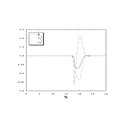
In Fig. 4 we plot the evolution of $\xi$, $c_{\rm S}^{2}$ and $c_{\rm T}^{2}$ for the model $p=X-ce^{-\lambda\phi}$ with the same model parameters and initial conditions as given in Fig. 1. During the scaling matter era in which $x_{3}$ is much smaller than of order unity [see Eq. (56)], we have that $|H\dot{f}|\ll 1$ and $|\ddot{f}|\ll 1$ giving $c_{\rm S}^{2}\simeq 1$ and $c_{\rm T}^{2}\simeq 1$. For the de-Sitter point (78) one can easily show that $c_{\rm S}^{2}=c_{\rm T}^{2}=1$. These properties are in fact confirmed in the numerical simulation of Fig. 4.

We find from Fig. 4 that $c_{\rm S}^{2}$ and $c_{\rm T}^{2}$ temporally become negative during the transition from the scaling matter era to the final de-Sitter era. This corresponds to the stage in which the contribution of the GB term is dominant. The perturbations exhibit exponential instabilities associated with the appearance of ghosts. The propagation speed of scalar perturbations can be modified in the presence of a matter fluid, but that of tensor perturbations is not affected. Hence the negative instability of tensor perturbations is robust even taking into account the contribution of the matter. This is consistent with the results of Ref. GOT in which the negative instability of tensor perturbations has been also found if inflationary solutions are constructed by the dominance of the GB term. In Fig. 4 we also find that the propagation speed of scalar perturbations temporally become superluminal.

For the model parameters given in Figs. 1 and 4 the propagation speed $c_{\rm T}$ becomes imaginary before the system reaches the present epoch (while $c_{\rm S}^{2}$ is positive). Meanwhile if we choose smaller values of $\mu$, it is possible to avoid reaching the negative values of $c_{\rm T}^{2}$. For smaller $\mu$, however, the minimum value of $w_{\rm eff}$ tends to be larger. Hence the exponential instability of tensor perturbations can be avoided at the expense of losing rapid accelerated expansion of the universe. It is of interest to find parameter ranges of $\lambda$ and $\mu$ which lead to positive $c_{\rm T}^{2}$ and also satisfy the observational constraints of $w_{\rm eff}$.

V Conclusions

In this paper we have discussed the viability of Gauss-Bonnet (GB) dark energy models which possess cosmological scaling solutions. In order to alleviate the coincident problem of dark energy, it is of interest to find a cosmological trajectory which is in a scaling regime ($\Omega_{\phi}/\Omega_{m}=$constant) during a matter era and finally exits to give rise to a late-time accelerated expansion. We have tried to understand the property of scalar-field dark energy models which allow such a possibility.

First we derived the form of the GB coupling together with the form of the scalar-field Lagrangian for the existence of scaling solutions by starting from a very general action given in Eq. (1). The form of the GB coupling has been found to be $f(\phi)\propto e^{\lambda\phi}$ together with the field Lagrangian density $p=Xg(Xe^{\lambda\phi})$, where $\lambda$ is defined in Eq. (16) and $g$ is an arbitrary function. The field Lagrangian density takes the same form as in the case where the GB coupling is absent.

We have also derived autonomous equations and fixed points for the scaling Lagrangian $p=Xg(Xe^{\lambda\phi})$ with the GB coupling $f(\phi)\propto e^{\mu\phi}$. When $\lambda=\mu$, we obtained the scaling solution characterised by $x_{1}=\sqrt{6}/[2(Q+\lambda)]$ and the scalar-field dominated solution characterised by $\Omega_{\phi}+\Omega_{{\rm GB}}=1$ without specifying any form of the Lagrangian. In this case, however, the solutions do not get away from the scaling matter regime to connect to a dark energy era. When $\mu>\lambda$ the presence of the GB term can lead to the exit from the scaling regime.

The GB term allows an interesting possibility to have a late-time de-Sitter fixed point. This point is present if the solutions for $gx_{1}^{2}=0$ and $x_{1}=0$ exist. The models which possess this de-Sitter solution are characterised by the form $g(Y)=(c_{0}-c/Y)f(Y)$, where $f(Y)$ is a function that approaches a constant as $x_{1}\to 0$. The ordinary field with an exponential potential (19) and the tachyon field with an inverse square potential (21) belong to this class, whereas the dilatonic ghost condensate model (20) does not.

We have studied cosmological evolution for the above two models in which the de-Sitter point is present. In the case of an ordinary field with an exponential potential one can in fact obtain a viable trajectory along which the scaling matter period is followed by the de-Sitter solution provided that $\mu>\lambda$ and $\lambda^{2}>3$ for $Q=0$. There is also an interesting possibility in which the effective equation of state $w_{\rm eff}$ temporarily becomes smaller than $-1$ because of the growth of the GB term. This is realized by choosing larger values of $\mu$, but it also corresponds to a shorter matter-dominated period. The late-time acceleration is possible even for $\lambda=\mu$ by using a scalar-field & GB dominated point ($\Omega_{\phi}+\Omega_{{\rm GB}}=1$), but in this case the contribution of the GB term is very small at the present epoch. Moreover we do not have a scaling matter era in this case, which is not a welcome feature in solving the coincidence problem.

The tachyon field has a de-Sitter fixed point, but in this case the scaling solution is absent for a non-relativistic background fluid ($w_{m}=0$) if $Q=0$. Hence we do not have a successful sequence of the scaling matter era and the de-Sitter expansion. If the coupling $Q$ is present, however, it is possible to realize this sequence when $\mu$ is larger than $\lambda$. The values of $Q$ are bounded from both above and below to get a scaling matter era with $w_{\rm eff}$ close to 0. An alternative approach to the problem discussed here can be provided by Renormalization Group (RG) equations. The scaling solution presented here turns out to be the fixed point of RG flow equations; the form of the field Lagrangian and the GB coupling are automatically fixed in this method sanjay .

We also discussed ghost conditions for the GB dark energy models by considering gravitational perturbations. For the ordinary field with an exponential potential we found that the propagation speeds of scalar and tensor modes can be imaginary during the transition from the scaling matter era to the final de-Sitter attractor. This is associated with the appearance of ghosts which lead to negative instabilities of perturbations. This ghost stage can be avoided by tuning the model parameters at the expense of obtaining a minimum effective equation of state closer to $-1$.

In this paper we have not studied local gravity constraints on the GB coupling ACD ; ACD2 . If the contribution of the GB coupling is large at present epoch, this may contradict with local gravity experiments unless an accidental cancellation occurs to avoid the large variation of effective gravitational constant. We leave future work for the construction of scaling GB dark energy models consistent with such constraints. We hope that the results obtained in this paper will be useful to find such viable models.

References

- (1) S. Perlmutter et al., Astrophys. J. 517, 565 (1999); A. G. Riess et al., Astron. J. 116, 1009 (1998); Astron. J. 117, 707 (1999); J. L. Tonry et al., Astrophys. J. 594, 1 (2003); R. A. Knop et al., Astrophys. J. 598, 102 (2003).
- (2) V. Sahni and A. A. Starobinsky, Int. J. Mod. Phys. D 9, 373 (2000); V. Sahni, Lect. Notes Phys. 653, 141 (2004); S. M. Carroll, Living Rev. Rel. 4, 1 (2001); T. Padmanabhan, Phys. Rept. 380, 235 (2003); P. J. E. Peebles and B. Ratra, Rev. Mod. Phys. 75, 559 (2003).
- (3) E. J. Copeland, M. Sami and S. Tsujikawa, arXiv:hep-th/0603057.
- (4) S. Weinberg, Rev. Mod. Phys. 61, 1 (1989).
- (5) Y. Fujii, Phys. Rev. D 26, 2580 (1982); L. H. Ford, Phys. Rev. D 35, 2339 (1987); C. Wetterich, Nucl. Phys B. 302, 668 (1988); B. Ratra and J. Peebles, Phys. Rev D 37, 321 (1988); Y. Fujii and T. Nishioka, Phys. Rev. D 42, 361 (1990); T. Chiba, N. Sugiyama and T. Nakamura, Mon. Not. Roy. Astron. Soc. 289, L5 (1997); R. R. Caldwell, R. Dave and P. J. Steinhardt, Phys. Rev. Lett. 80, 1582 (1998); I. Zlatev, L. M. Wang and P. J. Steinhardt, Phys. Rev. Lett. 82, 896 (1999); B. Boisseau, G. Esposito-Farese, D. Polarski and A. A. Starobinsky, Phys. Rev. Lett. 85, 2236 (2000).
- (6) T. Chiba, T. Okabe and M. Yamaguchi, Phys. Rev. D 62, 023511 (2000); C. Armendáriz-Picón, V. Mukhanov, and P. J. Steinhardt, Phys. Rev. Lett. 85, 4438 (2000); Phys. Rev. D 63, 103510 (2001).
- (7) A. Sen, JHEP 9910, 008 (1999); JHEP 0204, 048 (2002); M. R. Garousi, Nucl. Phys. B584, 284 (2000); Nucl. Phys. B 647, 117 (2002); G. W. Gibbons, Phys. Lett. B 537, 1 (2002); T. Padmanabhan, Phys. Rev. D 66, 021301 (2002); T. Padmanabhan and T. R. Choudhury, Phys. Rev. D 66, 081301 (2002); M. R. Garousi, M. Sami and S. Tsujikawa, Phys. Rev. D 70, 043536 (2004).
- (8) M. Gasperini, F. Piazza and G. Veneziano, Phys. Rev. D 65, 023508 (2002).
- (9) N. Arkani-Hamed, P. Creminelli, S. Mukohyama and M. Zaldarriaga, JCAP 0404, 001 (2004).
- (10) F. Piazza and S. Tsujikawa, JCAP 0407, 004 (2004).
- (11) P. G. Ferreira and M. Joyce, Phys. Rev. Lett. 79, 4740 (1997); Phys. Rev. D 58, 023503 (1998).
- (12) E. J. Copeland, A. R. Liddle and D. Wands, Phys. Rev. D 57, 4686 (1998).
- (13) A. P. Billyard, A. A. Coley and R. J. van den Hoogen, Phys. Rev. D 58, 123501 (1998); A. R. Liddle and R. J. Scherrer, Phys. Rev. D 59, 023509 (1999); J. P. Uzan, Phys. Rev. D 59, 123510 (1999); R. J. van den Hoogen, A. A. Coley and D. Wands, Class. Quant. Grav. 16, 1843 (1999); A. Nunes and J. P. Mimoso, Phys. Lett. B 488, 423 (2000); A. de la Macorra and G. Piccinelli, Phys. Rev. D 61, 123503 (2000); S. C. C. Ng, N. J. Nunes and F. Rosati, Phys. Rev. D 64, 083510 (2001); C. Rubano and J. D. Barrow, Phys. Rev. D 64, 127301 (2001); Z. K. Guo, Y. S. Piao, R. G. Cai and Y. Z. Zhang, Phys. Lett. B 576, 12 (2003); Z. K. Guo, Y. S. Piao and Y. Z. Zhang, Phys. Lett. B 568, 1 (2003); S. Mizuno, S. J. Lee and E. J. Copeland, Phys. Rev. D 70, 043525 (2004); E. J. Copeland, S. J. Lee, J. E. Lidsey and S. Mizuno, Phys. Rev. D 71, 023526 (2005); M. Sami, N. Savchenko and A. Toporensky, Phys. Rev. D 70, 123526 (2004); V. Pettorino, C. Baccigalupi and F. Perrotta, JCAP 0512, 003 (2005); L. Amendola, S. Tsujikawa and M. Sami, Phys. Lett. B 632, 155 (2006); Y. Gong, A. Wang and Y. Z. Zhang, Phys. Lett. B 636, 286 (2006).
- (14) S. Tsujikawa and M. Sami, Phys. Lett. B 603, 113 (2004).
- (15) S. Tsujikawa, Phys. Rev. D 73, 103504 (2006).
- (16) L. Amendola, M. Quartin, S. Tsujikawa and I. Waga, Phys. Rev. D 74, 023525 (2006).
- (17) T. Barreiro, E. J. Copeland and N. J. Nunes, Phys. Rev. D 61, 127301 (2000).
- (18) V. Sahni and L. M. Wang, Phys. Rev. D 62, 103517 (2000).
- (19) A. Albrecht and C. Skordis, Phys. Rev. Lett. 84, 2076 (2000).
- (20) A. A. Coley and R. J. van den Hoogen, Phys. Rev. D 62, 023517 (2000); S. A. Kim, A. R. Liddle and S. Tsujikawa, Phys. Rev. D 72, 043506 (2005).
- (21) A. R. Liddle, A. Mazumdar and F. E. Schunck, Phys. Rev. D 58, 061301 (1998).
- (22) J. E. Lidsey, D. Wands and E. J. Copeland, Phys. Rept. 337, 343 (2000); M. Gasperini and G. Veneziano, Phys. Rept. 373, 1 (2003)
- (23) I. Antoniadis, J. Rizos and K. Tamvakis, Nucl. Phys. B 415, 497 (1994); M. Gasperini, M. Maggiore and G. Veneziano, Nucl. Phys. B 494, 315 (1997); S. Foffa, M. Maggiore and R. Sturani, Nucl. Phys. B 552, 395 (1999); N. E. Mavromatos and J. Rizos, Phys. Rev. D 62, 124004 (2000); JHEP 0207, 045 (2002); C. Cartier, E. J. Copeland and R. Madden, JHEP 0001, 035 (2000); S. Tsujikawa, R. Brandenberger and F. Finelli, Phys. Rev. D 66, 083513 (2002); S. Tsujikawa, Class. Quant. Grav. 20, 1991 (2003).
- (24) E. Elizalde, S. Nojiri and S. D. Odintsov, Phys. Rev. D 70, 043539 (2004); S. Nojiri and S. D. Odintsov, Phys. Lett. B 595, 1 (2004); Phys. Rev. D 70, 103522 (2004); S. Nojiri, S. D. Odintsov and S. Tsujikawa, Phys. Rev. D 71, 063004 (2005).
- (25) S. Nojiri, S. D. Odintsov and M. Sasaki, Phys. Rev. D 71, 123509 (2005).
- (26) T. Koivisto and D. F. Mota, arXiv:astro-ph/0606078.
- (27) G. Calcagni, S. Tsujikawa and M. Sami, Class. Quant. Grav. 22, 3977 (2005); M. Sami, A. Toporensky, P. V. Tretjakov and S. Tsujikawa, Phys. Lett. B 619, 193 (2005).
- (28) B. M. N. Carter and I. P. Neupane, Phys. Lett. B 638, 94 (2006); JCAP 0606, 004 (2006); I. P. Neupane, arXiv:hep-th/0602097.
- (29) S. Nojiri and S. D. Odintsov, Phys. Lett. B 631, 1 (2005); arXiv:hep-th/0601213.
- (30) G. Cognola, E. Elizalde, S. Nojiri, S. D. Odintsov and S. Zerbini, Phys. Rev. D 73, 084007 (2006).
- (31) A. De Felice, M. Hindmarsh and M. Trodden, JCAP 0608, 005 (2006).
- (32) G. Calcagni, B. de Carlos and A. De Felice, Nucl. Phys. B 752, 404 (2006).
- (33) S. Nojiri, S. D. Odintsov and M. Sami, Phys. Rev. D 74, 046004 (2006).
- (34) S. Tsujikawa, Annalen Phys. 15, 302 (2006) [arXiv:hep-th/0606040].
- (35) A. K. Sanyal, arXiv:astro-ph/0608104.
- (36) K. Andrew, B. Bolen and C. A. Middleton, arXiv:hep-th/0608127.
- (37) L. Amendola, Phys. Rev. D 62, 043511 (2000).
- (38) L. Amendola, Phys. Rev. D 60, 043501 (1999).
- (39) B. Gumjudpai, T. Naskar, M. Sami and S. Tsujikawa, JCAP 0506, 007 (2005).
- (40) L. R. W. Abramo and F. Finelli, Phys. Lett. B 575, 165 (2003).
- (41) J. M. Aguirregabiria and R. Lazkoz, Phys. Rev. D 69, 123502 (2004).
- (42) E. J. Copeland, M. R. Garousi, M. Sami and S. Tsujikawa, Phys. Rev. D 71, 043003 (2005).
- (43) T. Koivisto and D. F. Mota, arXiv:hep-th/0609155.
- (44) A. G. Riess et al. [Supernova Search Team Collaboration], Astrophys. J. 607, 665 (2004).
- (45) C. J. Odman, A. Melchiorri, M. P. Hobson and A. N. Lasenby, Phys. Rev. D 67, 083511 (2003).
- (46) H. Kodama and M. Sasaki, Prog. Theor. Phys. Suppl. 78, 1 (1984); V. F. Mukhanov, H. A. Feldman and R. H. Brandenberger, Phys. Rept. 215, 203 (1992); B. A. Bassett, S. Tsujikawa and D. Wands, Rev. Mod. Phys. 78, 537 (2006).
- (47) J. c. Hwang and H. Noh, Phys. Rev. D 71, 063536 (2005).
- (48) Z. K. Guo, N. Ohta and S. Tsujikawa, arXiv:hep-th/0610336.
- (49) C. Bonvin, C. Caprini and R. Durrer, Phys. Rev. Lett. 97, 081303 (2006).
- (50) S. Jhingan et. al, work in progress.
- (51) L. Amendola, C. Charmousis and S. C. Davis, arXiv:hep-th/0506137.
- (52) L. Amendola, C. Charmousis and S. C. Davis, work in progress.