Discretized Gravity in 6D Warped Space

Florian Bauer^a, Tomas Hällgren^b, and Gerhart Seidl^c

Abstract

We consider discretized gravity in six dimensions, where the two extra dimensions have been compactified on a hyperbolic disk of constant curvature. We analyze different realizations of lattice gravity on the disk at the level of an effective field theory for massive gravitons. It is shown that the observed strong coupling scale of lattice gravity in discretized five-dimensional flat or warped space can be increased when the latticized fifth dimension is wrapped around a hyperbolic disk that has a non-trivial warp factor. As an application, we also study the generation of naturally small Dirac neutrino masses via a discrete volume suppression mechanism and discuss briefly collider implications of our model.

1 Introduction

Theories with gravity in a curved space-time background exhibit a number of intriguing features. The warped metric of the Randall-Sundrum (RS) models [1, 2], for example, allows to address the gauge hierarchy problem by considering our four-dimensional (4D) world as a sub-manifold of a five-dimensional (5D) anti de Sitter space (alternatively, see Ref. [3]). Apart from that, the AdS/CFT correspondence [4] suggests in warped geometries an amazing gauge-gravity duality. Moreover, in string compactifications with fluxes, strongly warped regions in space-time offer a wide range of new phenomenological and cosmological applications and serve here, in particular, as a useful device for moduli stabilization [5].

A strong space-time curvature is also beneficial when formulating lattice gravity as an effective field theory (EFT) [6, 7, 8] (for related work see, e.g., Ref. [9]). Although lattice gravity has, to lowest order in its interactions, a strong analogy to the gauge theory case [10, 11] it shows a radically different strong coupling behavior at the non-linear level. In 5D flat space, for instance, the ultraviolet (UV) strong coupling scale depends on the bulk volume, or infrared (IR) scale, via a so-called “UV/IR connection” that would forbid to take the large volume limit within a sensible EFT [7]. This UV/IR connection can, however, be avoided for discretized gravity in 5D warped space-time [12, 13] (for warped non-gravitational extra dimensions see, e.g., Refs. [14, 15, 16]), which has been shown to work in the manifestly holographic regime and admits to take the large volume limit.

In this paper, we consider a six-dimensional (6D) lattice gravity setup, where the two extra dimensions are compactified on a discretized hyperbolic disk. We first analyze a coarse-grained latticization of the hyperbolic disk and show that the UV strong coupling scale is essentially set by the inverse disk radius and becomes independent of the total number of lattice sites on the boundary. It turns out that, even in the large volume limit, all bounds from laboratory experiments, astrophysics, and cosmology on Kaluza-Klein (KK) gravitons are avoided whereas the model would still be testable at a collider. In a second example, we study a fine-grained latticization of the hyperbolic disk with nonzero warping. We determine approximately the complete mass spectrum and the wave-function profiles of the gravitons and estimate the local strong coupling scale on the disk. We find that the presence of the 6th dimension can yield the theory on the boundary sub-manifold of the disk more weakly coupled than in the corresponding 5D warped case with a single latticized extra dimension. We also analyze the action of a bulk right-handed neutrino in the coarse-grained model and show that a large curvature of the disk allows to generate small active Dirac neutrino masses via a volume suppression mechanism.

The paper is organized as follows. In Sec. 2, we introduce the extra-dimensional hyperbolic disk that is then coarsely discretized in Sec. 3, where we also discuss collider implications of the model. Next, in Sec. 4, we calculate the strong coupling scale for the coarse-grained latticization. In Sec. 5, we analyze the EFT for a fine-grained latticization with nonzero warping and demonstrate that the local strong coupling scale can be pushed to higher values when going from five to six dimensions. As an application, we present in Sec. 6 a mechanism for small Dirac neutrino masses in the coarse-grained model. Finally, in the Appendix, we derive the Fierz-Pauli Lagrangian on the hyperbolic disk.

2 6D warped hyperbolic space

Let us consider 6D general relativity compactified to four dimensions on an orbifold $K_{2}/Z_{2}$, where $K_{2}$ is a two-dimensional hyperbolic disk of constant negative curvature. We use capital Roman indices $M=0,1,2,3,5,6$ to label the 6D coordinates $x^{M}$ while Greek indices $\mu=0,1,2,3$ denote the usual 4D coordinates $x^{\mu}$. The 6D Minkowski metric is given by $\eta_{MN}=\textrm{diag}(1,-1,\dots,-1)$. A point on the hyperbolic disk $K_{2}$ is described by a pair of polar coordinates $(r,\varphi)$, where $r=x^{5}$ and $\varphi=x^{6}$ are the radial and the angular coordinates of the point, respectively; on $K_{2}$, the coordinates $r$ and $\varphi$ can take the values $r\in[0,L]$, where $L\geq 0$ and $\varphi\in[0,2\pi)$. We choose the coordinates such that $r$ is the geodesic or proper distance of the point $(r,\varphi)$ from the center, i.e., $L$ is the hyperbolic or proper radius of the disk. The orbifold $K_{2}/Z_{2}$ is obtained from $K_{2}$ by imposing on the angle $\varphi$ the orbifold projection $\varphi\rightarrow-\varphi$, which restricts the physical space on the disk to $(r,\varphi)\in[0,L]\times[0,\pi]$.

We assume that the disk is warped along the radial direction like in the 5D RS scenario and that the radial coordinate $r$ takes the role of the 5th dimension in the RS model. The 6D metric for the warped hyperbolic disk $\tilde{g}_{MN}$ is given by the line element

$$\textrm{d}s^{2}=e^{2\sigma(r)}g_{\mu\nu}(x,r,\varphi)\textrm{d}x^{\mu}\textrm{d}x^{\nu}-\textrm{d}r^{2}-\frac{1}{v^{2}}\,\textrm{sinh}^{2}(v\cdot r)\textrm{d}\varphi^{2},$$ (1)

where $1/v$ is the curvature radius of the disk with $v>0$, $g_{\mu\nu}(x,r,\varphi)$ is the 4D metric with $x\equiv(x^{\mu})$, and

$$\sigma(r)=-w\cdot r,$$ (2)

where $w$ is the curvature scale for the warping along the radial direction. We denote the components of the metric $\tilde{g}_{MN}$ in Eq. (1) by $\tilde{g}_{\mu\nu}=e^{2\sigma(r)}g_{\mu\nu}(x,r,\varphi)$, $\tilde{g}_{55}=-1$, and $\tilde{g}_{66}=-v^{-2}\textrm{sinh}^{2}(vr)$. This metric is defined for any values of $r\in[0,L]$, where the radius $L$ is finite but can be arbitrarily large. Like in RS I [1], we have assumed in Eq. (1) orbifold boundary conditions with respect to $r$ at the center $r=0$ and at the boundary of the disk at $r=L$. While we identify the UV brane with the center at $r=0$, we have IR branes residing at the orbifold fixed points on the boundary at $r=L$. The orbifold $K_{2}/Z_{2}$ with the definition of the coordinates and the location of the UV and IR branes is shown in Fig. 1.

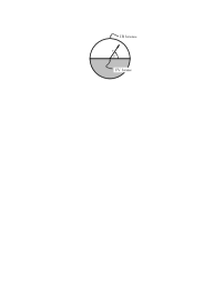
Figure 1: Physical space of the orbifold $K_{2}/Z_{2}$. Shown are the coordinates $(r,\varphi)$ of a point on the hyperbolic disk $K_{2}$. The orbifold projection $\varphi\rightarrow-\varphi$ identifies the upper half of $K_{2}$ with the lower half (gray shaded region). The disk is warped along the radial direction with the UV and IR branes located at the center and at the boundary of the disk, respectively.

In these coordinates, a concentric circle through a point $(r,\varphi)$ has a proper radius $r$ and a proper circumference $2\pi v^{-1}\textrm{sinh}(vr)$. The proper area of the corresponding disk is

$$A=\int\textrm{d}r\,\textrm{d}\varphi\sqrt{|\tilde{g}_{66}|}=4\pi v^{-2}\sinh^{2}{(vr/2)}.$$ (3)

For $vr\gg 1$, the circumference and the area of the circle thus grow exponentially with $r$.

It is interesting to compare our hyperbolic space with the Poincaré hyperbolic disk. Introducing a new radial coordinate $\hat{r}$ that is defined by $\textrm{d}r=(1-\frac{1}{4}v^{2}\hat{r}^{2})^{-1}\textrm{d}\hat{r}$, we find from Eq. (1) the Poincaré hyperbolic metric

$$\textrm{d}s^{2}=e^{2\sigma(\hat{r})}g_{\mu\nu}(x,\hat{r},\varphi)\textrm{d}x^{\mu}\textrm{d}x^{\nu}-\frac{1}{(1-\frac{1}{4}v^{2}\hat{r}^{2})^{2}}(\textrm{d}\hat{r}^{2}+\hat{r}^{2}\textrm{d}\varphi^{2}),$$ (4)

where $\sigma(\hat{r})$ is obtained by replacing in $\sigma(r)=-wr$ the coordinate $r$ by $r(\hat{r})$. The metric in Eq. (4) has a coordinate singularity at $\hat{r}=2/v$ corresponding to spatial infinity $r\rightarrow\infty$. The coordinate $\hat{r}$ is thus restricted to the interval $\hat{r}\in[0,2/v)$ whereas $\varphi\in[0,2\pi)$. The polar coordinates $(\hat{r},\varphi)$ define the Poincaré hyperbolic disk, which is shown in Fig. 2 for the example of a semi-regular $\{6,6,8\}$ tessellation.

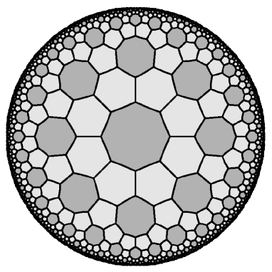
Figure 2: Poincaré hyperbolic disk with semi-regular $\{6,6,8\}$ tessellation [17].

In Eq. (4), we have

$$\sigma(\hat{r})=-\frac{w}{v}\,\textrm{log}\left(\frac{1+\frac{v}{2}\hat{r}}{1-\frac{v}{2}\hat{r}}\right).$$ (5)

In Fig. 2, the proper radius and proper circumference of a concentric circle through a point $(\hat{r},\varphi)$ are $-\sigma(\hat{r})/w$ and $2\pi\hat{r}/(1-\frac{1}{4}v^{2}\hat{r}^{2})$, which both diverge when approaching spatial infinity at $\hat{r}=2/v$. In the rest of the paper, we will, however, always use the coordinates $(r,\varphi)$ and take the metric as given in Eq. (1).

On the hyperbolic disk, we write the gravitational action as

$$\mathcal{S}=M_{6}^{4}\int\textrm{d}^{6}x\,\sqrt{|\tilde{g}|}(\tilde{R}-2\Lambda),$$ (6)

where $\tilde{g}\equiv\det\tilde{g}_{MN}$ and it is implied that the integration over $r$ and $\varphi$ is restricted to the hyperbolic disk. In Eq. (6), $M_{6}$ is the 6D Planck scale, $\Lambda$ the bulk cosmological constant, and $\tilde{R}=\tilde{g}^{MN}\tilde{R}_{MN}$ is the 6D curvature scalar, where $\tilde{R}_{MN}$ denotes the 6D Ricci tensor. The relevant parts of the action can be written in the form

$$\mathcal{S} = M_{6}^{4}\int\textrm{d}^{6}x\sqrt{|g|}\Big{[}e^{2\sigma(r)}R_{\rm 4D}-\frac{1}{4}\tilde{g}^{55}\partial_{r}(e^{2\sigma(r)}g_{\mu\nu})(g^{\mu\nu}g^{\alpha\beta}-g^{\mu\alpha}g^{\nu\beta})\partial_{r}(e^{2\sigma(r)}g_{\alpha\beta})$$ (7)

$$\qquad\qquad\qquad\quad\>\,-\frac{1}{4}\tilde{g}^{66}\partial_{\varphi}(e^{2\sigma(r)}g_{\mu\nu})(g^{\mu\nu}g^{\alpha\beta}-g^{\mu\alpha}g^{\nu\beta})\partial_{\varphi}(e^{2\sigma(r)}g_{\alpha\beta})\Big{]},$$

where we have defined $|g|\equiv e^{-8\sigma(r)}|\tilde{g}|$ and $R_{\rm 4D}$ is the 4D curvature scalar with respect to the 4D metric $g_{\mu\nu}$ (for a definition of $R_{\rm 4D}$ and a derivation of Eq. (7), see Appendix A).

We expand $g_{\mu\nu}$ in terms of small fluctuations around 4D Minkowski space by replacing $g_{\mu\nu}=\eta_{\mu\nu}+h_{\mu\nu}$. To quadratic order, the kinetic part of the graviton Lagrangian density is then, after partial integration, explicitly found to be of the Fierz-Pauli form [18, 19]

$$\mathcal{S}_{\textrm{lin}} = M_{6}^{4}\int\textrm{d}^{6}x\,v^{-1}\textrm{sinh}(vr)\Big{[}\frac{1}{4}e^{2\sigma(r)}(\partial^{\mu}h^{\nu\kappa}\partial_{\mu}h_{\nu\kappa}-\partial^{\mu}h\partial_{\mu}h-2h^{\mu}h_{\mu}+2h^{\mu}\partial_{\mu}h)$$ (8)

$$\qquad\qquad\qquad\qquad+\frac{1}{4}e^{4\sigma(r)}(\partial_{r}h_{\mu\nu})(\eta^{\mu\nu}\eta^{\alpha\beta}-\eta^{\mu\alpha}\eta^{\nu\beta})(\partial_{r}h_{\alpha\beta})$$

$$\qquad\,\,+\frac{1}{4}e^{4\sigma(r)}v^{2}\textrm{sinh}^{-2}(vr)(\partial_{\varphi}h_{\mu\nu})(\eta^{\mu\nu}\eta^{\alpha\beta}-\eta^{\mu\alpha}\eta^{\nu\beta})(\partial_{\varphi}h_{\alpha\beta})\Big{]},$$

where $h={h^{\mu}}_{\mu}$ and $h_{\nu}=\partial^{\mu}h_{\mu\nu}$. In the analysis of the 5D model in Ref. [7], it has proven useful to neglect the 4D vector, scalar, and radion degrees of freedom. For simplicity, we have adopted here a similar gauge where we set $h_{5M}=h_{6M}=0$, for $M=0,1,\dots,6$.

Let us now consider the 6D Einstein tensor $\tilde{G}_{MN}=\tilde{R}_{MN}-\frac{1}{2}\tilde{g}_{MN}\tilde{R}$ for a flat 4D background $g_{\mu\nu}=\eta_{\mu\nu}$, in which case $\tilde{G}_{MN}$ is on diagonal form $\tilde{G}_{MN}=\textrm{diag}(\tilde{G}_{11},\tilde{G}_{22},\dots,\tilde{G}_{66})$. Up to corrections of the order $e^{-vr}$, the components of $\tilde{G}_{MN}$ asymptote in the IR very quickly to $\tilde{G}_{11}=\tilde{G}_{22}=\tilde{G}_{33}=-\tilde{G}_{00}=(3vw-6w^{2}-v^{2})e^{-2wr}$, $\tilde{G}_{55}=4vw-6w^{2}$, and $\tilde{G}_{66}=-10w^{2}v^{-2}\textrm{sinh}^{2}(vr)$. In this limit, the 6D Einstein equations can be formally satisfied by (i) adding to the gravitational action in Eq. (6) a “matter” action

$$\mathcal{S}_{\textrm{m}}=M_{6}^{4}\int\textrm{d}^{6}x\sqrt{|\tilde{g}|}\tilde{g}^{AB}n_{AB},$$ (9)

where $n_{AB}$ denotes the tensor $n_{AB}\equiv-\tilde{G}_{AB}$, and by (ii) setting the bulk cosmological constant $\Lambda$ in Eq. (6) equal to $\Lambda=-\frac{1}{2}\tilde{G}^{A}_{\,\,\,A}$. Note that for zero warping $w=0$, we obtain the exact result that the tensor $n_{AB}$ becomes constant throughout the bulk.

In what follows, we will view discrete gravitational extra dimensions as a tool to explore general relativity without the need to explicitly solve Einstein’s equations [12]. Here, the massive gravitons in the compactified theory can be understood in terms of a graph consisting of sites and links called “theory space”, and it is not necessary to find, e.g., the gravitational source for an action of the type in Eq. (9).

3 Coarse-grained discretization

In this section, we consider a discretization of the hyperbolic disk $K_{2}$ with a metric as given in Eq. (1). In particular, we analyze here the case where the warping along the radial direction is set to zero, i.e., it is $w=0$, while the curvature radius $v$ is non-vanishing. The general case, with both $w\neq 0$ and $v\neq 0$, will be studied later in Sec. 5.

3.1 Latticization

Let us consider the coarse-grained latticization of the hyperbolic disk $K_{2}$ that is described by the diagram in Fig. 3.

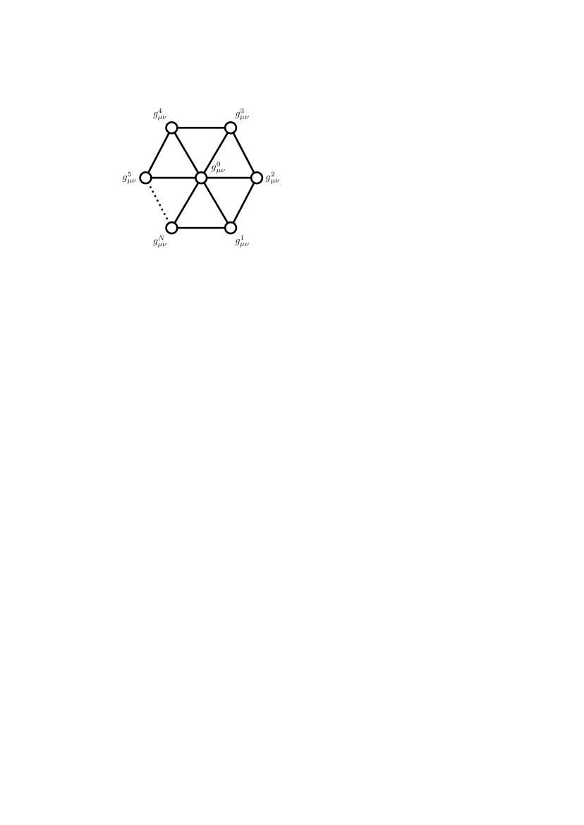
Figure 3: Coarse-grained discretization of the hyperbolic disk $K_{2}$. The circles represent the sites and are labeled as $i=0,1,2,\dots,N$. On each site $i$ lives a graviton field $g_{\mu\nu}^{i}$ and two neighboring sites $i$ and $j$ are connected by a link $(i,j)_{\textrm{link}}$ (solid lines).

The diagram is spanned by $N$ sites located on the boundary of $K_{2}$, which are labeled as $i=1,2,\dots,N$ with the identification $i+N\equiv i$, while the center of the disk is represented by a single site $i=0$. The sites on the boundary of $K_{2}$ are evenly spaced on a concentric circle with proper radius $L$ around the central site $i=0$ residing at the origin, i.e., the $i$th site on the boundary has polar coordinates $(r,\varphi)=(L,i\cdot\Delta\varphi)$, where $\Delta\varphi=2\pi/N$. In Fig. 3, two sites $i$ and $i+1$ on the boundary are connected by a link $(i,i+1)_{\textrm{link}}$ while the site $i=0$ in the center is connected to all $N$ sites on the boundary by the links $(0,i)_{\textrm{link}}$. To implement a lattice gravity theory in terms of this triangulation, we will throughout interpret the sites and links following the theory of massive gravitons in Refs. [6, 7, 8]. Here, each site $i$ is equipped with its own metric $g^{i}_{\mu\nu}$, which can be expanded around flat space as $g^{i}_{\mu\nu}=\eta_{\mu\nu}+h^{i}_{\mu\nu}$, where $\eta_{\mu\nu}$ is the usual 4D Minkowski metric. In a naive latticization of the linearized action $\mathcal{S}_{\textrm{lin}}$ in Eq. (8), we then replace the derivatives on the sites as

$$\partial_{\varphi}h_{\mu\nu}\rightarrow\frac{1}{\Delta\varphi}(h_{\mu\nu}^{i+1}-h_{\mu\nu}^{i}),\quad\partial_{r}h_{\mu\nu}\rightarrow\frac{1}{L}(h^{i}_{\mu\nu}-h_{\mu\nu}^{0}),$$ (10)

which gives the Fierz-Pauli graviton mass terms

$$\mathcal{S}_{\textrm{FP}} = M_{4}^{2}\int\textrm{d}^{4}x\,\sum_{i=1}^{N}\left[m_{*}^{2}(h_{\mu\nu}^{i}-h_{\mu\nu}^{0})(\eta^{\mu\nu}\eta^{\alpha\beta}-\eta^{\mu\alpha}\eta^{\nu\beta})(h_{\alpha\beta}^{i}-h_{\alpha\beta}^{0})\right.$$ (11)

$$\qquad\qquad\qquad\left.+m^{2}(h_{\mu\nu}^{i+1}-h_{\mu\nu}^{i})(\eta^{\mu\nu}\eta^{\alpha\beta}-\eta^{\mu\alpha}\eta^{\nu\beta})(h_{\alpha\beta}^{i+1}-h_{\alpha\beta}^{i})\right],$$

where $M_{4}$ is the “local” universal 4D Planck scale on each of the sites whereas $m_{*}$ and $m$ respectively denote the proper inverse lattice spacings in radial and angular direction. To relate $M_{4}$ to $M_{6}$, note that Eq. (7) yields upon discretization

$$M_{6}^{4}\int\textrm{d}^{6}x\,\sqrt{|\tilde{g}|}\rightarrow\frac{M_{6}^{4}A}{N}\sum_{i=0,1}^{N}\int\textrm{d}^{4}x\,\sqrt{|g_{4}|},$$ (12)

where $A$ is the proper area of the disk from Eq. (3) with $r=L$ and $g_{4}=\textrm{det}\,g_{\mu\nu}$. In Eq. (12), it is understood that the sum starts from $i=0$ for the kinetic terms and from $i=1$ for the mass terms, respectively. The mass scales in Eq. (11) can then be matched as

$$m_{*}=\frac{1}{L},\quad m=\frac{Nv}{2\pi\,\textrm{sinh}(vL)},\quad M_{4}^{2}=\frac{M_{6}^{4}A}{N},\quad M_{\rm Pl}^{2}=M_{6}^{4}A=M_{4}^{2}N,$$ (13)

where $M_{\rm Pl}\simeq 10^{18}\>{\rm GeV}$ is the usual 4D Planck scale of the low-energy theory. In the basis $(h_{\mu\nu}^{0},h_{\mu\nu}^{1},\dots,h_{\mu\nu}^{N})$, the $(N+1)\times(N+1)$ graviton mass matrix reads

$$M_{\textrm{g}}^{2}=m_{*}^{2}\left(\begin{matrix}N&-1&-1&\cdots&-1\\ -1&1\\ -1&&1\\ \vdots&&&\ddots\\ -1&&&&1\end{matrix}\right)+m^{2}\left(\begin{matrix}0&0&0&\dots&0\\ 0&2&-1&&-1\\ 0&-1&2&\ddots\\ \vdots&&\ddots&\ddots&-1\\ 0&-1&&-1&2\end{matrix}\right),$$ (14)

where the blank entries are zero. Diagonalization of $M_{\textrm{g}}^{2}$ leads to the graviton mass spectrum

$$M_{0}^{2}=0,\quad M_{n}^{2}=m_{*}^{2}+4m^{2}{\textrm{sin}}^{2}\frac{\pi n}{N},\quad M_{N}^{2}=(N+1)m_{\ast}^{2},$$ (15)

where $n=1,2,\dots,N-1$. Note that the spectrum in Eq. (15) has been described previously for the gauge theory case [21, 22]. Denoting the $n$th mass eigenstate with mass $M_{n}$ as given in Eq. (15) by $\hat{H}_{\mu\nu}^{n}$, the mass eigenstates can be written as

$$\hat{H}^{0}_{\mu\nu} = \frac{1}{\sqrt{N+1}}(1,1,1,\dots,1),$$ (16a)

$$\hat{H}^{n}_{\mu\nu} = \frac{1}{\sqrt{N}}(0,1,e^{{\textrm{i}}\frac{2n\pi}{N}},e^{{\textrm{i}}\frac{4n\pi}{N}},\dots,e^{{\textrm{i}}\frac{2(N-1)n\pi}{N}}),$$ (16b)

$$\hat{H}^{N}_{\mu\nu} = \frac{1}{\sqrt{N(N+1)}}(N,-1,-1,\dots,-1),$$ (16c)

where in Eq. (16b) the index $n$ runs over $n=1,2,\dots,N-1$ and we have, for definiteness, taken $N$ to be even. The mass eigenstates include a zero mode $\hat{H}_{\mu\nu}^{0}$ with flat profile. Note that the $N-1$ massive eigenstates $\hat{H}_{\mu\nu}^{n}$ in Eq. (16b) are all exactly located on the boundary while the $N$th massive mode $\hat{H}_{\mu\nu}^{N}$ in Eq. (16c) is peaked in the center. The tower of masses $M_{n}$ belonging to the states $\hat{H}_{\mu\nu}^{n}$ reproduces for $n\ll N$ a linear KK-type spectrum $\sim m\cdot n/N$ that is sitting on top of $m_{\ast}^{2}$. From Eq. (13), we also observe that the limit $m\ll m_{\ast}$ can be realized for $N\gg 1$ with a sufficiently large value of $vL$. In this case, the $N-1$ states in Eq. (16b) become practically degenerate with mass $m_{*}$ and the $N$th mode $\hat{H}_{\mu\nu}^{N}$ becomes very heavy, i.e., $M_{N}\gg m_{\ast}$.

3.2 Phenomenological implications

It has been recently demonstrated that large extra dimensions can be hidden in “multi-throat” configurations where the occurrence of KK gravitons is delayed to energies that are much higher than the inverse radius of the extra dimension [23]. Such a multi-throat geometry is found in our coarse-grained model as a special case in the limit $m\rightarrow 0$. Therefore, by the same arguments as in Ref. [23], the corrections to Newton’s law in the coarse-grained model become only important when the distance between two test masses is shorter than a critical radius $r_{\textrm{crit}}\simeq m_{*}^{-1}\>{\textrm{log}}\>N$. For $N\simeq 10^{30}$, e.g., we could thus have, like in large extra dimensions, the local Planck scale on the sites lowered down to $M_{4}\simeq M_{\textrm{Pl}}/\sqrt{N}\simeq 1\>\textrm{TeV}$ while for $m_{*}\gtrsim 100\>{\textrm{MeV}}$ all current bounds on large extra dimensions from Cavendish-type experiments [24], astrophysics [25], and cosmology [26] are avoided.

The collider implications for the direct production of KK gravitons $\hat{H}^{n}$ in $e^{+}+e^{-}\rightarrow\gamma+\hat{H}^{n}$ and $p+p\rightarrow{\rm jet}+\hat{H}^{n}$ reactions can be determined like in the large extra dimensional scenario: Standard Model (SM) matter located on a single site $k$ on the boundary of the disk interacts with gravity as

$$\mathcal{S}_{\rm int}\approx\frac{1}{M_{\text{Pl}}}\int d^{4}x\,T^{\mu\nu}\Big{(}\sum_{n=1}^{N-1}e^{-{\rm i}2\pi k\cdot n/N}\hat{H}^{n}_{\mu\nu}+\hat{H}^{0}_{\mu\nu}+\frac{1}{\sqrt{N}}\hat{H}^{N}_{\mu\nu}\Big{)}+{\rm h.c.},$$ (17)

where $T^{\mu\nu}$ is the SM stress-energy tensor. We have in this expression for large $N$ used the approximation $N+1\approx N$. We see that SM matter has $1/M_{\textrm{Pl}}$ suppressed couplings to the graviton zero mode and to the $N-1$ quasi-degenerate modes, whereas the couplings to the heavy mode are even suppressed by a factor $1/\sqrt{N}M_{\rm Pl}$. For example, assuming $N=10^{30}$ sites and inverse lattice spacings $m_{*}=14\>\textrm{TeV}$ and $m=0.14\>\textrm{GeV}$, we find for a center-of-momentum (CoM) energy $E_{\textrm{CoM}}=14.1\>\textrm{TeV}$ and a quark energy $E_{\rm q}\gtrsim 10^{2}\>\textrm{GeV}$ that the cross section for the production of an individual KK graviton via the parton subprocess $q+g\rightarrow q+\hat{H}^{n}$ is $\sigma\sim 10^{-30}\>\textrm{pb}$. This is, of course, not observable at a collider (as a detectability requirement of signal above background we take $\sigma\gtrsim 1-100\>\textrm{fb}$ [27]). But summing over the high multiplicity of $N=10^{30}$ states, we actually have here a total cross section $\sigma_{\rm total}\sim 1\>\textrm{pb}$, which could give a signal at the LHC. The signal would be a jet plus missing transverse energy. Of course, a proper treatment of the reaction $p+p\rightarrow{\rm jet}+\hat{H}^{n}$ should take into account the summation over the parton subprocesses with the appropriate parton distribution functions, which is, however, beyond the scope of this paper.

For a choice of parameters $N=10^{30}$, $m_{*}=1.0\>\textrm{TeV}$, $m=1.0\>\textrm{GeV}$, $E_{\rm CoM}=1.01\>\textrm{TeV}$, and a lower cutoff for the photon energy $E_{\gamma}\gtrsim 10\>\textrm{GeV}$, the cross section for the production of an individual KK mode via $e^{+}+e^{-}\rightarrow\gamma+\hat{H}^{n}$ is $\sigma\sim 10^{-29}\>\textrm{pb}$, which results in a total cross section of the order $\sigma_{\rm total}\sim 8\>\textrm{pb}$ and could, e.g., be observable at the ILC. The signal would be a photon plus missing transverse energy. In Fig. 4, we present the cross sections for this reaction as a function of $E_{{\rm CoM}}$. We give the results for $m_{*}=1000$ GeV, $m_{*}=1250$ GeV, and $m_{*}=1500$ GeV. In all cases, we have chosen $N=10^{30}$, $m=1$ GeV, and a lower cutoff for the photon energy $E_{\gamma}\gtrsim 10\>\textrm{GeV}$. We have also made a comparison with the ADD scenario [3] for 2 large extra dimensions and a fundamental scale $M_{f}=2.5$ TeV. The coarse-grained model has a qualitatively different behavior compared to large extra dimensions. The sharp peak close to $E_{\rm CoM}\sim m_{*}$ is due to the nearly degenerate spectrum located around $E_{\rm CoM}\sim m_{*}$. Below $E_{\rm CoM}\sim m_{*}$, the cross section is zero because of the large mass gap between the zero mode and the first excited mode.

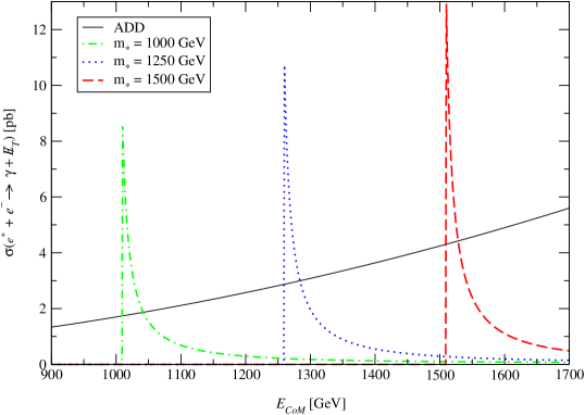
Figure 4: Cross section $\sigma(e^{+}+e^{-}\rightarrow\gamma+E\kern-4.95003pt\raise 0.19376pt\hbox{/}_{T})$ in units of pb versus $E_{{\rm CoM}}$ in GeV. Shown is the cross section for the coarse-grained model with $m_{*}=1000$ GeV (dash-dotted), $m_{*}=1250$ GeV (dotted), and $m_{*}=1500$ GeV (dashed). In all cases, we have chosen $m=1$ GeV and $N=10^{30}$ sites. For comparison, we have also presented a typical ADD model with 2 extra dimensions and $M_{f}=2.5$ TeV (solid line). We have also made a kinematic cut by taking $E_{\gamma}\gtrsim 10$ GeV. The coarse-grained model gives a signal that is qualitatively different from usual large extra dimensions. The sharp peak close to $E_{{\rm CoM}}\sim m_{*}$ is due to the nearly degenerate spectrum located around $E_{{\rm CoM}}\sim m_{*}$. Below $E_{{\rm CoM}}\sim m_{*}$, the cross section drops to zero because of the mass-gap in the disk model.

In addition, the exchange of virtual KK modes could influence the cross sections for some SM processes which we will, however, not discuss in further detail here.

4 Effective theory

In this section, we will study the strong coupling behavior of the coarse-grained model presented in Sec. 3.1, where we use throughout the EFT for massive gravitons introduced in Refs. [6, 7, 8]. Before turning to the complete latticized disk, however, it is instructive to consider first the strong coupling scales in two of its sub-geometries. The first one is represented by the boundary of the disk, which we will call the “circle” geometry. The second one is obtained by removing the links on the boundary, and we will henceforth call this theory space the “star” geometry (for studies of related geometries, see, e.g., Ref. [28]). First, in Secs. 4.1, 4.2, and 4.3, we determine the strong coupling scale by restricting to the Goldstone boson sector. Then, in Sec. 4.4, we discuss the strong coupling scale that is actually seen by an observer localized on a single site on the boundary of the disk.

4.1 Strong coupling in the circle geometry

To implement the EFT on the latticized hyperbolic disk $K_{2}$, we replace in Eq. (10) the differences $h^{i}_{\mu\nu}-h^{j}_{\mu\nu}$ between the graviton fields on two sites $i$ and $j$ that are connected by a link $(i,j)_{\textrm{link}}$ according to

$$h_{\mu\nu}^{i}-h_{\mu\nu}^{j}\,\,\rightarrow\,\,g_{\mu\nu}^{i}-\partial_{\mu}Y_{i,j}^{\alpha}\partial_{\nu}Y_{i,j}^{\beta}g^{j}_{\alpha\beta},$$ (18a)

where $$Y_{i,j}^{\mu}$$ denotes a link field that can be written as

$$Y_{i,j}^{\mu}(x_{\mu})=x^{\mu}+A_{i,j}^{\mu}(x_{\mu})+\partial^{\mu}\phi_{i,j}(x_{\mu}),$$ (18b)

in which $A_{i,j}^{\mu}$ and $\phi_{i,j}$ represent the vector and scalar components of the Goldstone bosons that restore general coordinate invariances in the EFT. For a detailed description of the technique for restoring general coordinate invariances, see Refs. [6, 7, 8].

The circle geometry is obtained from the coarse-grained latticized disk in Sec. 3.1 by assuming $m_{*}=0$ and $m$ nonzero. Since this reduces the model to the 5D lattice gravity theory discussed in Ref. [7], we will only give a short review of this case here.

The kinetic Lagrangian of the gravitons is found by specializing in Eqs. (18) the links $(i,j)_{\textrm{link}}$ to the case $(i,j)_{\textrm{link}}=(i,i-1)_{\textrm{link}}$, where $i=2,\ldots,N,N+1$. As a consequence, we obtain from the Fierz-Pauli mass terms in Eq. (11) for the circle geometry the action

$$\mathcal{S}_{\rm circle}=\mathcal{S}_{\rm FP}+\int{\rm d}^{4}x\>M_{4}^{2}\sum_{i=1}^{N}(h^{i}_{\mu\nu}\Box h^{i}_{\mu\nu}+m^{2}[(h^{i}_{\mu\nu}-h^{i-1}_{\mu\nu})\Box\phi_{i,i-1}+(\Box\phi_{i,i-1})^{3}]).$$ (19)

The kinetic mixing between the gravitons and scalar Goldstones can be eliminated by partial integration and a subsequent Weyl rescaling, which produces proper kinetic terms for the Goldstones [6]. As shown in Ref. [7], this EFT for massive gravitons has a cutoff

$$\Lambda_{\rm circle}=(N^{3/2}M_{4}m_{1}^{4})^{1/5}=(M_{\rm Pl}m^{4}/N^{3})^{1/5},$$ (20)

where $m_{1}=m/N$ is the mass of the lightest massive graviton, and we have used that the usual 4D Planck scale $M_{\rm Pl}\simeq 10^{18}\>{\rm GeV}$ is related to the local 4D Planck scale on the sites $M_{4}$ by $M_{\rm Pl}=\sqrt{N}M_{4}$ [see Eq. (13)]. The strong coupling scale $\Lambda_{\rm circle}$ depends on the number of lattice sites $N$, i.e., on the circumference $R=Nm^{-1}$ of the circle. The fact that the UV scale $\Lambda_{\rm circle}$ depends on the IR scale $R$ has been called UV/IR connection and restricts in a sensible EFT the possible number of sites to a maximal value $N_{\rm max}=(M_{4}^{2}mR^{3})^{1/8}$ [7].

4.2 Strong coupling in the star geometry

The star geometry arises from the coarse-grained disk model by setting the parameters $m=0$ and $m_{*}\neq 0$. Note that this geometry is similar to the multi-throat configuration which has been analyzed for the gauge theory case in Ref. [23]. In contrast to Sec. 4.1, we specialize here to the case in which the links $(i,j)_{\textrm{link}}$ in Eqs. (18) are $(i,j)_{\textrm{link}}=(i,0)_{\textrm{link}}$, where $i=1,2,\dots,N$. We then get from the Fierz-Pauli mass terms in Eq. (11) the action

$$\mathcal{S}_{\rm star}=\mathcal{S}_{\rm FP}+\int{\rm d}^{4}x\>M_{4}^{2}(h^{0}_{\mu\nu}\Box h^{0}_{\mu\nu}+\sum_{i=1}^{N}(h^{i}_{\mu\nu}\Box h^{i}_{\mu\nu}+m_{*}^{2}[(h^{0}_{\mu\nu}-h^{i}_{\mu\nu})\Box\phi_{0,i}+(\Box\phi_{0,i})^{3}])),$$ (21)

where we have also included the kinetic terms of the gravitons. In Eq. (21), the terms $m_{*}^{2}(h_{\mu\nu}^{0}-h_{\mu\nu}^{i})\Box\phi_{0,i}$ can be written as a $(N+1)\times N$ kinetic matrix which is proportional to

$$\left(\begin{matrix}1&1&1&\dots&1\\ -1&0&0&\dots&0\\ 0&-1&0&\dots&0\\ 0&0&-1&\dots&0\\ \vdots&\vdots&\vdots&\ddots&\vdots\\ 0&0&0&\dots&-1\end{matrix}\right),$$ (22)

where the rows and columns are spanned by $(h_{\mu\nu}^{0},h_{\mu\nu}^{1},\dots,h_{\mu\nu}^{N})$ and $(\phi_{0,1},\phi_{0,2},\dots,\phi_{0,N})$, respectively. To determine here the strong coupling scale, we express the gravitons on the boundary as the linear combinations $h^{i}_{\mu\nu}=\frac{1}{\sqrt{N}}\sum_{n=1}^{N}e^{{\rm i}2\pi i\cdot n/N}{H^{\prime}}^{n}_{\mu\nu}$, where we have introduced the fields ${H^{\prime}}^{n}_{\mu\nu}=H_{\mu\nu}^{n}$, for $n=2,3,\dots,N-1$, with $H_{\mu\nu}^{n}$ from Eq. (16b) while ${H^{\prime}}^{N}_{\mu\nu}$ is in the basis of Eqs. (16) given by the $(N+1)$-component vector ${H^{\prime}}^{N}_{\mu\nu}=\frac{1}{\sqrt{N}}(0,1,1,\dots,1)$. Similarly, we expand the scalar components of the Goldstone fields belonging to the links $(i,0)_{\textrm{link}}$ as $\phi_{i,0}=\frac{1}{\sqrt{N}}\sum_{n=1}^{N}e^{{\rm i}2\pi i\cdot n/N}\Phi_{n}$. The matrix in Eq. (22) gets then transformed to

$$\left(\begin{matrix}0&0&0&\dots&\sqrt{N}\\ -1&0&0&\dots&0\\ 0&-1&0&\dots&0\\ 0&0&-1&\dots&0\\ \vdots&\vdots&\vdots&\ddots&\vdots\\ 0&0&0&\dots&-1\end{matrix}\right),$$ (23)

where the rows and columns have been written in the bases $(h^{0}_{\mu\nu},{H^{\prime}}^{1}_{\mu\nu},{H^{\prime}}^{2}_{\mu\nu},\dots,{H^{\prime}}^{N}_{\mu\nu})$ and $(\Phi_{1},\Phi_{2},\dots,\Phi_{N})$, respectively. Let us next perform a rotation by the angle ${\rm arctan}(\sqrt{N})$ acting in the 2-dimensional subspace $(h_{\mu\nu}^{0},{H^{\prime}}^{N}_{\mu\nu})$ from the left on the first and last rows of the matrix in Eq. (23). This rotates away the entry $\sqrt{N}$ in the top-right corner and introduces new basis vectors via $(h^{0}_{\mu\nu},{H^{\prime}}^{N}_{\mu\nu})\rightarrow(H^{0}_{\mu\nu},H^{N}_{\mu\nu})$, with $H^{0}_{\mu\nu}$ and $H^{N}_{\mu\nu}$ as defined in Eqs. (16a) and (16b), respectively. We can then approximate the action in Eq. (21) by

$$\mathcal{S}_{\rm star} = \mathcal{S}_{\rm FP}+\int{\rm d}^{4}x\>M_{4}^{2}\Big{[}h^{0}_{\mu\nu}\Box h^{0}_{\mu\nu}+\sum_{n=1}^{N}\Big{(}H^{n}_{\mu\nu}\Box H^{-n}_{\mu\nu}$$ (24)

$$- m_{*}^{2}H_{\mu\nu}^{n}\Box\Phi_{-n}\Big{)}+\sum_{n,m=1}^{N}\Big{(}\frac{m_{*}^{2}}{\sqrt{N}}(\Box\Phi_{n})(\Box\Phi_{m})(\Box\Phi_{-n-m})\Big{)}\Big{]},$$

where we have defined $H_{\mu\nu}^{-n}=H_{\mu\nu}^{N-n}$ and $\Phi_{-n}=\Phi_{N-n}$. From this equation, we read off the graviton fields in canonical normalization $\hat{H}^{n}_{\mu\nu}=M_{4}H_{\mu\nu}^{n}$, and, consequently, the canonically normalized scalar Goldstone modes are $\hat{\Phi}_{n}=M_{4}m_{*}^{2}\Phi_{n}$. In Eq. (24), we thus have

$$M_{4}^{2}\frac{m_{*}^{2}}{\sqrt{N}}(\Box\Phi_{n})(\Box\Phi_{m})(\Box\Phi_{-n-m})=\frac{1}{\sqrt{N}M_{4}m_{*}^{4}}(\Box\hat{\Phi}_{n})(\Box\hat{\Phi}_{m})(\Box\hat{\Phi}_{-n-m}).$$ (25)

From the amplitude for $\hat{\Phi}_{n}-\hat{\Phi}_{m}$ scattering, we hence find for the star geometry the strong coupling scale

$$\Lambda_{\rm star}=(\sqrt{N}M_{4}m_{*}^{4})^{1/5}=(M_{\rm Pl}m_{*}^{4})^{1/5},$$ (26)

which is independent from the number of sites $N$ on the boundary. This is different from the circle geometry since the discrete radial derivatives in Eq. (21) do not depend on $N$. Therefore, the UV/IR connection problem from the circle geometry is absent in the star geometry. Note that the strong coupling scale in Eq. (26) appears to be what we would naively expect in the theory of a single massive graviton with mass $m_{*}$ [6]. However, as we will see later in Sec. 4.4, the strong coupling scale actually seen by a 4D brane-localized observer on the boundary is in the limit $m_{\ast}\rightarrow M_{4}$ smaller than in the theory of a single massive graviton.

4.3 Strong coupling on the disk

In the disk model of Sec. 3.1, the links form a mesh which would generally imply the presence of additional uneaten pseudo-Nambu-Goldstone bosons. These bosons, however, can acquire large masses from invariant plaquette terms that are added to the action [6]. In our model, we will therefore assume that these scalars decouple and estimate the strong coupling scale on the disk $\Lambda_{\rm disk}$ only from the scattering of the modes that are eaten by the gravitons.

The combination of $\mathcal{S}_{\rm circle}$ and $\mathcal{S}_{\rm star}$ gives, using the notation of Sec. 4.2, in momentum basis the total action of the disk

$$\mathcal{S}_{\rm disk} = \mathcal{S}_{\rm FP}+\int{\rm d}^{4}x\>M_{4}^{2}\Big{[}h^{0}_{\mu\nu}\Box h^{0}_{\mu\nu}+\sum_{n=1}^{N}\Big{(}H^{n}_{\mu\nu}\Box H^{-n}_{\mu\nu}$$ (27)

$$- H_{\mu\nu}^{n}\Box(m_{*}^{2}\Phi_{-n}+m^{2}(1-e^{-\textrm{i}2\pi\cdot n/N})\Phi^{\prime}_{-n})\Big{)}$$

$$+ \sum_{n,k=1}^{N}\Big{(}\frac{m_{*}^{2}}{\sqrt{N}}(\Box\Phi_{n})(\Box\Phi_{k})(\Box\Phi_{-n-k})+\frac{m^{2}}{\sqrt{N}}(\Box\Phi^{\prime}_{n})(\Box\Phi^{\prime}_{k})(\Box\Phi^{\prime}_{-n-k})\Big{)}\Big{]},$$

where $\Phi_{n}$ and $H^{n}_{\mu\nu}$ are defined as in Eq. (24) while the $\Phi^{\prime}_{n}$ are related to the scalar Goldstones $\phi_{i,i-1}$ of the circle geometry by $\phi_{i,i-1}=\frac{1}{\sqrt{N}}\sum_{n=1}^{N}e^{{\rm i}2\pi i\cdot n/N}\Phi^{\prime}_{n}$. From Eq. (27), we hence find that the Goldstones $\Phi_{n}^{\circ}$ which become the scalar longitudinal components of the gravitons $H_{\mu\nu}^{n}$ are, for $n\ll N$, approximately given by

$$\Phi_{n}^{\circ}\approx m_{\ast}^{2}\Phi_{n}+2\pi\frac{n}{N}m^{2}\Phi^{\prime}_{n}.$$ (28)

Thus, for large $N$, the field $\Phi_{n}^{\circ}$ becomes dominantly composed of $\Phi_{n}$, whereas $\Phi^{\prime}_{n}$ makes up almost entirely the uneaten linear combination orthogonal to $\Phi^{\circ}_{n}$. Consider now in Eq. (27) the tri-linear derivative coupling term involving the field $\Phi^{\prime}_{n}$. In the pure circle geometry discussed in Sec. 4.1, the coupling of this term becomes strong for large $N$ and is responsible for the UV/IR connection. In our disk model, however, the linear combination orthogonal to $\Phi^{\circ}_{n}$ decouples. In this limit, since the admixture of $\Phi^{\prime}_{n}$ to $\Phi_{n}^{\circ}$ is only of the order $\sim 1/N$, the tri-linear coupling of $\Phi^{\prime}_{n}$ in Eq. (27) picks up a suppression factor $\sim 1/N^{3}$, when expressed in terms of the canonically normalized fields $\hat{\Phi}^{\circ}_{n}=M_{4}\Phi_{n}^{\circ}$, and takes approximately the form

$$\frac{m^{2}}{\sqrt{N}}(\Box\Phi^{\prime}_{n})(\Box\Phi^{\prime}_{k})(\Box\Phi^{\prime}_{-n-k})\rightarrow\frac{m^{8}}{N^{7/2}M_{4}m_{\ast}^{12}}(\Box\hat{\Phi}^{\circ}_{n})(\Box\hat{\Phi}^{\circ}_{k})(\Box\hat{\Phi}^{\circ}_{-n-k}),$$ (29)

where we have assumed that $n,k\sim 1\ll N$. Unless $m$ is not too large compared to $m_{\ast}$, the dominant contribution to the massive graviton scattering is therefore given by the tri-linear derivative coupling of the fields $\Phi_{n}$ in Eq. (27) (see Fig. 5).

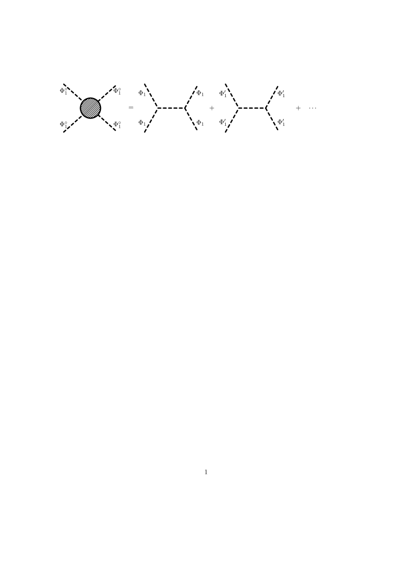
Figure 5: Contributions to the scattering amplitude of the lightest massive graviton in the coarse-grained disk model. For large $N$, the scalar $\Phi^{\circ}_{1}$ is dominantly composed of $\Phi_{1}$, and the relative contribution from $\Phi^{\prime}_{1}-\Phi^{\prime}_{1}$ scattering becomes suppressed by a factor $\sim 1/N^{6}$.

This coupling is similar to the term in Eq. (24) that sets the strong coupling scale in the star geometry. For $N\rightarrow\infty$, the strong coupling scale of the disk model $\Lambda_{\rm disk}$ thus converges to

$$\Lambda_{\rm disk}\rightarrow\Lambda_{\rm star}=(M_{\rm Pl}m_{\ast}^{4})^{1/5}.$$ (30)

The EFT for massive gravitons in our disk model does therefore not suffer from the UV/IR connection of the circle sub-geometry and thus allows to take the large $N$ limit. Again, the strong coupling scale in Eq. (30) has been estimated by considering the self-interactions of the Goldstone bosons only. Next, in Sec. 4.4, we will take the coupling to matter into account and determine the strong coupling scale that is actually observed on a single site on the boundary of the disk.

4.4 Inclusion of matter

The strong coupling scales given for the star and the disk model in Eqs. (26) and (30) are, of course, deceptive, since they have been derived by looking at the Goldstone boson sector alone. To find the actual strong coupling scale as seen by an observer, we have to take into account the coupling of the Goldstone modes to SM matter. In what follows, we shall therefore consider SM matter located at a single site $k$ of the boundary, which interacts with gravity via the action $\mathcal{S}_{\text{int}}$ as given in Eq. (17). After an appropriate Weyl rescaling (for details see Refs. [6, 13]), $\mathcal{S}_{\text{int}}$ leads to the following interaction between the Goldstone bosons and matter:

$$\mathcal{S}^{\Phi}_{\text{int}}\approx\frac{1}{M_{\text{Pl}}}\int d^{4}x\Big{(}\sum_{n=1}^{N-1}e^{-{\rm i}2\pi k\cdot n/N}\hat{\Phi}_{-n}T+\frac{1}{\sqrt{N}}\hat{\Phi}_{0}T\Big{)}+{\rm h.c.},$$ (31)

where $T=\text{Tr}(T_{\mu\nu})$ and we have approximated $N+1\approx N$. Note that the coupling of $T$ to an individual Goldstone boson $\hat{\Phi}_{n}$ is suppressed by a factor $1/M_{\text{Pl}}$, but the sum over the high multiplicity of Goldstones can lower the strong coupling scales estimated in Secs. 4.2 and 4.3 significantly. SM fermions, for example, see strong coupling effects via processes of the types shown in Fig. 6.

Figure 6: Scattering of SM fermions via Goldstone modes. In the diagrams (a) and (b), we have $n,k=0,1,2,\dots,N$, and $k=l+m\;\text{mod}\,N$. The high multiplicity of internal states [$N$ for (a) and $N^{2}$ for (b)] introduces an upper bound on the actually observed strong coupling scale of the order of the local Planck scale $\lesssim M_{4}$.

From dimensional analysis, we estimate for the diagrams (a) and (b) in Fig. 6 that the strong coupling scales as seen by a SM observer become roughly

$$\text{Diagram (a)}\>:\>\Lambda_{\text{disk}}\rightarrow M_{4},\qquad\text{Diagram (b)}\>:\>\Lambda_{\text{disk}}\rightarrow\sqrt{M_{4}m_{\ast}}.$$ (32)

The actual strong coupling scale is therefore lower than that of the theory of a single massive graviton. However, since the strong coupling scales in Eq. (32) are, for a fixed local Planck scale $M_{4}$, independent from the number of sites $N$ on the boundary, the UV/IR connection problem is still absent – even after taking into account the high multiplicity of Goldstone bosons that couple to SM matter. When taking the limit $m_{\ast}\rightarrow M_{4}$, we find for diagram (b) in Eq. (32) that the strong coupling scale seen by an observer becomes $\Lambda_{\text{disk}}\rightarrow M_{4}$, that means, the actually observed strong coupling scale $\Lambda_{\text{disk}}$ can be as large as the local Planck scale $M_{4}$ on the sites of the boundary.

5 Fine-grained discretization

In this section, we will consider a refinement of the discretization of the hyperbolic disk described in Sec. 3. Different from our earlier discussion, however, we will now assume that the disk is strongly warped along the radial direction and consider finally also a nonzero warping in angular direction.

5.1 Structure of the graph

In choosing a refined discretization of the hyperbolic disk, we will, in what follows, confine ourselves to the class of graphs that are collectively represented by Fig. 7, where we interpret the sites and links as in Sec. 3.1.

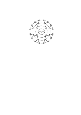
Figure 7: Fine-grained discretization of the hyperbolic disk. The graph shows the special case $\ell=2$ and $k_{\rm max}=4$. Angular links are represented as dashed lines and radial links as solid lines.

The sites are placed on concentric circles (dashed lines) around a site in the center of the disk. Starting from the innermost circle and going outward, the circles are labeled as $k=1,2,\dots,k_{\rm max}$, where the outermost circle, labeled by $k_{\rm max}$, is identified with the boundary of the disk. Fig. 7 depicts the special case $k_{\rm max}=4$.

Let us now specify the structure of the graph in more detail. We distinguish between two types of links: “angular” and “radial” links. In Fig. 7, the angular links connect neighboring sites on the same circle and are shown as dashed curved lines; the radial links connect neighboring sites that are not on the same circle and are drawn as solid straight lines.

The site in the center is connected with $\ell$ radial links to the sites on the first circle. Every site on the $k$th circle, where $1\leq k<k_{\rm max}$, is connected by $\ell$ radial links to the nearest $\ell$ sites on the next outer circle with label $k+1$. In Fig. 7, we have the special case $\ell=2$. To maximize the symmetry of the graph, we assume that all sites on a given circle are evenly spaced and that the links emanating outward from any given site on some inner circle with label $k<k_{\rm max}$ are always symmetrically arranged with respect to a 2-fold mirror symmetry axis through this site and the center of the disk. In what follows, we will, for simplicity and unless otherwise mentioned, specialize to the case $\ell=2$ as in Fig. 7 but leave $k_{\rm max}$ a free positive integer parameter. The generalization to $\ell>2$ is then straightforward. On the $k$th circle, we hence have $N_{k}\equiv 2^{k}$ sites, and the total number of sites on the first $k$ circles is $N_{k}^{\rm total}\equiv 2^{k+1}-1$. For later notational convenience, we denote by $N_{0}^{\rm total}=N_{0}=1$ the number of sites (only one) in the center. We wish to emphasize that the exponential growth of lattice sites, when moving from the center outward on the disk, is a salient feature of our graph that will play an important role in the study of the EFT in Sec. 5.6.

Similar to the 5D case in Ref. [12], we assume that the radial geodesic coordinates of the sites are integer multiples of a common proper radial lattice spacing $a_{r}$ and take the values

$$r_{k}=k\cdot a_{r},$$ (33)

where $k=0,1,2,\dots,k_{\textrm{max}}$, i.e., the $k$th circle has a proper radius $r_{k}$. We define $m_{*}\equiv 1/a_{r}$ as the inverse radial lattice spacing between two adjacent circles. Furthermore, since the sites on each given circle are evenly spaced, we define the lattice spacing in $\varphi$ direction between two neighboring sites on the $k$th circle as $a_{\varphi,k}=2\pi\,\textrm{sinh}(vr_{k})/(vN_{k})$, where $2\pi\,\textrm{sinh}(vr_{k})/v$ is the proper circumference of the $k$th circle. The inverse lattice spacing in $\varphi$ direction on the $k$th circle will then be written as $m_{k}\equiv 1/a_{\varphi,k}$, which is in general $k$-dependent.

To simplify further the discussion as much as possible, we will, in what follows, go to an approximation in which all radial links have the same universal proper length $a_{r}$. This is, of course, an arbitrarily good approximation for the set of radial links that radiate outward from the $k$th circle when $k\gg 1$ and $vL\ll 1$. However, in our approximation, we even assume that all the $N_{k}^{\textrm{total}}-1$ radial links on the disk have a common proper length $a_{r}$, irrespective of their position on the disk or the size of the curvature radius.

5.2 Radial warping

Let us now consider the implementation of a nonzero warping along the radial direction of the refined discretized hyperbolic disk introduced in Sec. 5.1. The graph we are concerned with is of the type given in Fig. 7, where the number of circles $k_{\rm max}$ can be arbitrary. In this section, we will, for simplicity, neglect the effect of the angular links (dashed lines) and assume that the graviton masses are generated only by the radial links (solid lines). As we will show in Sec. 5.5, the angular links can be easily taken into account in full generality for the complete disk model and do not have significant impact on the relevant properties of the model with radial links only.

Each site on the disk can be specified by an index pair $(k,j)$, where $k$ is the label of the circle where the site is located and $j=1,2,\dots,N_{k}$ labels (e.g., in clockwise direction) all the sites on this circle. The site in the center carries the index pair $(0,1)$. The metric living on the site $(k,j)$ is written as $g^{k,j}_{\mu\nu}=\eta_{\mu\nu}+h^{k,j}_{\mu\nu}$, where $h^{k,j}_{\mu\nu}$ is the graviton field on this site. We adopt a similar notation in momentum space and denote the canonically normalized graviton mass eigenstates by $\hat{H}^{k,j}_{\mu\nu}$, where $k=1,2,\dots,k_{\rm max}$ and $j=1,2,\dots,N_{k}$ while $\hat{H}_{\mu\nu}^{0,1}$ is the zero mode. The mass eigenvalue belonging to $\hat{H}^{k,i}_{\mu\nu}$ will be denoted by $\lambda_{k,i}$.

To specify the labeling of the sites more exactly, consider Fig. 8, which is another way of representing the inner part of the disk in Fig. 7, where the center appears now at the bottom of the graph and the concentric circles are shown as dashed horizontal lines.

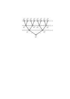
Figure 8: Sub-graph of the discretized hyperbolic disk obtained by truncating the disk at $k_{\textrm{max}}=3$. The horizontal dashed lines represent segments from the concentric circles with labels $k=1,2,3$. The labeling of the sites as $(k,i)$ is made explicit for the associated metrics $g_{\mu\nu}^{k,i}$ (see text).

The radial links are again drawn as straight solid lines. In the above notation, any given site $(k,i)$ on the $k$th circle, where $k=0,1,2,\dots,k_{\textrm{max}}-1$, is connected via two radial links with two nearest neighboring sites $(k+1,j_{1})$ and $(k+1,j_{2})$ on the next outer circle. The indices $j_{1}$ and $j_{2}$ are recursively defined as functions of the index $i$ by setting $j_{1}=2(i-1)+1$ and $j_{2}=2(i-1)+2$. Starting with the label $(0,1)$ for the center, this prescription fixes completely the assignment of labels for all sites on the circle by requiring the indices $i$ in $(k,i)$ to be ordered, e.g., in clockwise direction on the disk. The labeling is shown explicitly in Fig. 8 for the fields $g_{\mu\nu}^{k,i}$ living on the sites $(k,i)$.

To introduce the warping along the radial direction of the fine-grained latticized disk, we proceed exactly like in the discretized 5D RS model in Ref. [12] and replace in the linearized gravitational action in Eq. (8), e.g., the derivatives in the $r$ direction by

$$e^{-2wr}\partial_{r}h_{\mu\nu}\rightarrow\frac{1}{a_{r}}e^{-2wka_{r}}(h_{\mu\nu}^{k,j}-h_{\mu\nu}^{k-1,i}),$$ (34)

where it is understood that the sites $(k-1,i)$ and $(k,j)$, with $k=1,2,\dots,k_{\textrm{max}}$, are nearest neighbors on adjacent circles connected by a radial link. It is convenient to introduce a dimensionless number $\epsilon<1$, which is related to the warp factor by $\epsilon\equiv e^{-wa_{r}}$. Since from each site in the interior of the disk exactly two radial links are pointing outward, the index $j$ in Eq. (34) can be either $j=2(i-1)+1$ or $j=2(i-1)+2$. We thus obtain for the discretized action on the warped hyperbolic disk

$$\mathcal{S}_{\textrm{lin}}=\int{\rm d}^{4}x\>M_{4}^{2}\sum_{k=0}^{k_{\textrm{max}}}\sum_{i=1}^{N_{k}}\epsilon^{2k}h^{k,i}_{\mu\nu}\Box h^{k,i}_{\mu\nu}+\mathcal{S}_{\textrm{FP}},$$ (35)

where $\mathcal{S}_{\textrm{FP}}$ are the Fierz-Pauli mass terms

$$\mathcal{S}_{\textrm{FP}} = M_{4}^{2}\int\textrm{d}^{4}x\,\sum_{k=1}^{k_{\rm max}}\sum_{i=1}^{N_{k-1}}m_{*}^{2}\epsilon^{4k}\Big{[}(h_{\mu\nu}^{k-1,i}-h_{\mu\nu}^{k,n_{i}})(\eta^{\mu\nu}\eta^{\alpha\beta}-\eta^{\mu\alpha}\eta^{\nu\beta})(h_{\alpha\beta}^{k-1,i}-h_{\alpha\beta}^{k,n_{i}})$$ (36)

$$\qquad\qquad\qquad+(h_{\mu\nu}^{k-1,i}-h_{\mu\nu}^{k,n_{i}+1})(\eta^{\mu\nu}\eta^{\alpha\beta}-\eta^{\mu\alpha}\eta^{\nu\beta})(h_{\alpha\beta}^{k-1,i}-h_{\alpha\beta}^{k,n_{i}+1})\Big{]},$$

in which, according to our labeling, the index $n_{i}$ is given by $n_{i}=2(i-1)+1$, where $i=1,2,\dots,N_{k-1}$. From the kinetic terms in Eq. (35), we find that $M_{k}\equiv M_{4}\epsilon^{k}$ is the local Planck scale on each site on the $k$th circle. In the basis of canonically normalized fields $\hat{h}^{k,i}_{\mu\nu}=M_{4}\epsilon^{k}h^{k,i}_{\mu\nu}$, we find from the Fierz-Pauli mass terms that the mass matrix element between two fields $\hat{h}_{\mu\nu}^{k,i}$ and $\hat{h}_{\mu\nu}^{l,j}$ is given by

$$M_{(k,i)(l,j)}=\frac{1}{a_{r}^{2}}\epsilon^{2(l+1)}[(2\epsilon^{2}+\epsilon^{-2})\delta_{k,l}\delta_{i,j}-\epsilon^{-1}\delta_{k+1,l}(\delta_{n_{i},j}+\delta_{n_{i}+1,j})-\epsilon\,\delta_{k-1,l}\delta_{\lceil i/2\rceil,j}],$$ (37)

where it is assumed that $k>0$, while $n_{i}$ is as in Eq. (36), and $\lceil\dots\rceil$ is the ceiling function. The matrix element $M_{(0,1)(l,j)}$ is obtained by dropping in Eq. (37) the quantity $\epsilon^{-2}$. In what follows, we will work in the “rough, local flat space approximation” of Ref. [12], where the product $wa_{r}$ is moderately small, i.e., $wa_{r}<1$. In this approximation, the mass matrix in Eq. (37) reduces to

$$M_{(k,i)(l,j)}\approx\frac{1}{a_{r}^{2}}\epsilon^{2(l+1)}[(2+\epsilon^{-2})\delta_{k,l}\delta_{i,j}-\delta_{k+1,l}(\delta_{n_{i},j}+\delta_{n_{i}+1,j})-\delta_{k-1,l}\delta_{\lceil i/2\rceil,j}],$$ (38)

where $k>0$. To arrive at Eq. (38), we have set in Eq. (37) $\epsilon,\epsilon^{2}=1$ but kept $\epsilon^{-2}$ and the higher powers $\epsilon^{2l}$ which can be small for $l\gg 1$. The matrix element $M_{(0,1),(l,j)}$ is in this approximation obtained from Eq. (38) by dropping $\epsilon^{-2}$. Note that this mass matrix is what one would expect in the corresponding gauge theory case [14, 15, 16].

Let us now comment on the range of parameters we are interested in. Like in the RS model, we will assume that the usual 4D low energy Planck scale $M_{\textrm{Pl}}\simeq 10^{18}\>\textrm{GeV}$ is given by the local Planck scale $M_{4}$ on the UV brane, i.e., we set $M_{4}\approx M_{\textrm{Pl}}$, which holds approximately as long as $\epsilon\cdot\ell\ll 1$, say, if $\epsilon\cdot\ell\lesssim 0.5$. For definiteness, we can, e.g., take the inverse radial lattice spacing $m_{\ast}\simeq(0.05)\times M_{4}$, assume that the small expansion parameter is $\epsilon\simeq 0.1$, and suppose that the curvature scale for the warping $w$ is somewhat smaller than the fundamental scale, i.e., $w\simeq(0.1)\times M_{\textrm{Pl}}$. To realize for these parameters, e.g., the RS I model with the SM on one of the sites on the boundary of the disk, we need on the boundary a local Planck scale $M_{k_{\textrm{max}}}=\epsilon^{k_{\textrm{max}}}M_{\textrm{Pl}}\simeq 1\>\textrm{TeV}$, which implies that in this case the disk has a proper radius that is roughly $k_{\textrm{max}}=\mathcal{O}(10)$ units $a_{r}$ wide. For our special case with $\ell=2$, we would then have $N_{k_{\textrm{max}}}=\mathcal{O}(10^{4})$ sites on the boundary.

If we want that $m_{\ast}$ becomes as large as $m_{\ast}=M_{4}\approx M_{\textrm{Pl}}$, while keeping the same number of sites on the boundary and $w\simeq(0.1)\times M_{\textrm{Pl}}$, we can “smooth out” our graph by inserting between each pair of neighboring circles roughly $20$ extra circles on which the number of sites $N_{k}$ grows sufficiently slowly when moving outward on the disk. This is achieved by formally replacing in the above example $\epsilon\rightarrow\epsilon^{1/20}=(0.1)^{1/20}$ and $\ell\rightarrow\ell^{1/20}=2^{1/20}$, in which case we would have $N_{k}=\ell^{k/20}$ and a proper radius that is $k_{\textrm{max}}\simeq\mathcal{O}(10^{2})$ units $M_{4}^{-1}$ wide.

5.3 Spectrum for a subgraph

Before analyzing the masses and eigenstates of the gravitons in the model for an arbitrary number of circles $k_{\textrm{max}}$, let us first study the spectrum for the subgraph in Fig. 8. From Eq. (38), we find in the basis $(\hat{h}_{\mu\nu}^{0,1},\hat{h}_{\mu\nu}^{1,1},\hat{h}_{\mu\nu}^{1,2},\hat{h}_{\mu\nu}^{2,1},\hat{h}_{\mu\nu}^{2,2},\hat{h}_{\mu\nu}^{2,3},\hat{h}_{\mu\nu}^{2,4})$ for the graviton mass matrix

$$M_{g}^{2}=m_{\ast}^{2}\epsilon^{2}\left(\begin{matrix}2&-1&-1&0&0&0&0\\ -1&1+2\epsilon^{2}&0&-\epsilon^{2}&-\epsilon^{2}&0&0\\ -1&0&1+2\epsilon^{2}&0&0&-\epsilon^{2}&-\epsilon^{2}\\ 0&-\epsilon^{2}&0&\epsilon^{2}&0&0&0\\ 0&-\epsilon^{2}&0&0&\epsilon^{2}&0&0\\ 0&0&-\epsilon^{2}&0&0&\epsilon^{2}&0\\ 0&0&-\epsilon^{2}&0&0&0&\epsilon^{2}\\ \end{matrix}\right),$$ (39)

where we have truncated the graph in Fig. 8 at the dashed line labeled by $k=2$. In what follows, we will determine the masses and mass eigenstates of the gravitons to leading order in perturbation theory following the example of the warped gauge theory case in Refs. [14, 23].

In the following, we choose a convention where the mass eigenvalue $\lambda_{k,i}$ belonging to $\hat{H}^{k,i}_{\mu\nu}$ measures the actual mass in multiples of $m_{\ast}^{2}$. The mass eigenstates of the matrix in Eq. (39) contain a flat zero mode

$$\hat{H}^{0,1}_{\mu\nu}=\frac{1}{\sqrt{7}}(1,1,1,1,1,1,1) : \lambda_{0,1}=0$$ (40a)

and two heavy modes

$$\hat{H}^{1,1}_{\mu\nu}=\frac{1}{\sqrt{2}}(0,-1,1,0,0,0,0) : \lambda_{1,1}=\epsilon^{2},$$ (40b)

$$\hat{H}^{1,2}_{\mu\nu}=\frac{1}{\sqrt{6}}(-2,1,1,0,0,0,0) : \lambda_{1,2}=3\epsilon^{2},$$ (40c)

where we have listed in each line also the eigenvalue corresponding to each eigenstate. Observe that the zero mode has an exactly flat wave-function profile whereas the two heavy modes are more localized toward the center of the disk. Furthermore, the spectrum contains the following three degenerate states

$$\hat{H}^{2,j}_{\mu\nu}=\frac{1}{2}(0,0,0,1,e^{{\rm i}2\pi j/4},e^{{\rm i}4\pi j/4},e^{{\rm i}6\pi j/4}) : \lambda_{2,j}=\epsilon^{4},$$ (40d)

where $$j=1,2,3$$, as well as the slightly heavier mode

$$\hat{H}^{2,4}_{\mu\nu}=\frac{1}{\sqrt{84}}(-4,-4,-4,3,3,3,3) : \lambda_{2,4}=\frac{7}{3}\epsilon^{4}.$$ (40e)

It is important to note that the mode profile in Eq. (40e) and the flat profile of the zero mode $\hat{H}^{0,1}_{\mu\nu}$ in Eq. (40a) are only a result of going in Eq. (38) to the rough, local flat space approximation. We will discuss the differences to the exact profiles in the following section.

5.4 Spectrum for the general case

Let us now consider the graviton spectrum for an arbitrary number of concentric circles $k_{\textrm{max}}$ in the rough, local flat space approximation of Sec. 5.2. We determine the eigenvalues and eigenstates of the graviton mass matrix to leading order in perturbation theory like in Sec. 5.3. In this general case, we thus find that the graviton mass matrix has a flat zero mode

$$\hat{H}^{0,1}_{\mu\nu}=\frac{1}{\sqrt{N_{k_{\rm max}}^{\rm total}}}(1,1,\ldots,1) : \lambda_{0,1}=0$$ (41)

and two heavy modes

$$\hat{H}^{1,1}_{\mu\nu}=\frac{1}{\sqrt{2}}(0,1,e^{{\rm i}\pi},0,\ldots,0) : \lambda_{1,1}=\epsilon^{2},$$ (42)

$$\hat{H}^{1,2}_{\mu\nu}=\frac{1}{\sqrt{6}}(-2,1,1,0,\ldots,0) : \lambda_{1,2}=3\epsilon^{2}.$$ (43)

In addition, there are for each circle with label $k=2,3,\ldots,k_{\rm max}$ in total $N_{k}-1$ degenerate modes that read

$$\hat{H}^{k,j}_{\mu\nu}=\frac{1}{\sqrt{N_{k}}}(\underbrace{0,\ldots,0}_{N_{k-1}^{\rm total}},\underbrace{1,e^{{\rm i}2\pi j/N_{k}},e^{{\rm i}4\pi j/N_{k}},\ldots,e^{{\rm i}2\pi j(N_{k}-1)/N_{k}}}_{N_{k}},0,\ldots,0) : \lambda_{k,j}=\epsilon^{2k},$$ (44)

where $j=1,2,\ldots,N_{k}-1$. These modes are all located on the $k$th circle. For each $k=2,3,\dots,k_{\rm max}$, this set of $N_{k}-1$ states is accompanied by a single slightly heavier mode which has an eigenvalue $\lambda_{k,N_{k}}\approx 2\epsilon^{2k}$ and is approximately given by

$$\hat{H}^{k,N_{k}}_{\mu\nu}=\frac{1}{\sqrt{N_{k}^{\rm total}}}(\underbrace{-1,\ldots,-1}_{N_{k-1}^{\rm total}},\underbrace{1,\ldots,1}_{N_{k}},0,\ldots,0) : \lambda_{k,N_{k}}\approx 2\epsilon^{2k}.$$ (45)

Note that, to leading order, these modes vanish outside the $k$th circle. As in Sec. 5.3, these “delocalized” profiles and the flat zero mode $\hat{H}_{\mu\nu}^{0,1}$ in Eq. (41) are only an artifact from working in the rough, local flat space approximation. In Fig. 9, a numerical calculation shows that the original mass matrix in Eq. (37) in fact reproduces a zero mode that is, as expected from the RS model, localized on the UV brane. Also the slightly heavier modes in Eq. (45) become actually localized on single circles. The spectrum and wave-function profiles of the gravitons for the general case are summarized in Table 1.

${\rm mass}/m_{*}^{2}$	$\#\,{\rm of}\,{\rm modes}$	${\rm wavefunction}$
$0$	$1$	Eq. (41)
$\epsilon^{2}$	$1$	Eq. (42)
$3\epsilon^{2}$	$1$	Eq. (43)
$\epsilon^{2k}$	$N_{k}-1$	Eq. (44)
$\approx 2\epsilon^{2k}$	$1$	Eq. (45)

Table 1: Mass spectrum and wave-function profiles for the gravitons in the rough, local flat space approximation, taking into account radial links only. Here, $N_{k}=2^{k}$ and $k=2,3,\ldots,k_{\rm max}$.

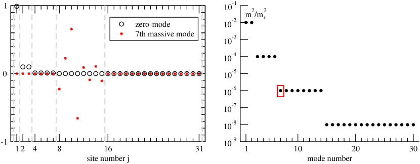
Figure 9: According to the “exact” mass matrix in Eq. (37), the left plot shows for $k_{\rm max}=4$ and $\epsilon=0.1$ the exact mode profiles of the zero mode (drawn as circles) and the 7th massive mode (drawn as stars). The latter would in the rough, local flat space approximation correspond to the mode in Eq. (45). The vertical dashed lines separate the sites on each circle, which illustrates that the zero mode is localized near the UV brane ($j=1$) and that the 7th mode has support only on the third circle ($j=8,\dots,15$). The right plot shows the “exact” mass spectrum, where the 7th massive mode is marked by a box and the zero mode has been omitted.

5.5 Effect of angular links

We can include the effect of the angular links on the total graviton mass matrix in Sec. 5.4 by adding to each sub-block spanned by the fields on the $k$th circle a matrix of the form

$$M^{k}_{ij}=m_{k}^{2}\epsilon^{2k}(2\delta_{i,j}-\delta_{i-1,j}-\delta_{i+1,j}),$$ (46)

where $i,j=1,2,\dots,N_{k}$ and $m_{k}$ is the proper inverse lattice spacing on the $k$th circle as defined in Sec. 5.1. The inclusion of angular links in the fine-grained model is therefore similar in effect to what happens in the example of the coarse-grained model in Sec. 3.1. Switching on the angular links leaves the zero mode unaffected but changes the masses of the degenerate modes $\hat{H}^{k,j}_{\mu\nu}$ in Eq. (44) as

$$m_{\ast}^{2}\lambda_{k,j}\rightarrow m_{\ast}^{2}\epsilon^{2k}+4m_{k}^{2}\epsilon^{2k}\sin^{2}\frac{j\pi}{N},$$ (47)

where $j=1,2,\ldots,N_{k}$. This is the analog of Eq. (15).

5.6 Local strong coupling scale

Let us now consider the local strong coupling scale on the discretized hyperbolic disk. In determining the strong coupling scale, we will restrict here ourselves first to the Goldstone boson sector. Later, in Sec. 5.7, we will take the coupling of the Goldstone bosons to matter into account and discuss the strong coupling scale that is actually experienced by a SM observer localized on a single site on the boundary of the disk. By the same arguments as in Sec. 4.3, we will restrict ourselves here again to the case where only the effect of the radial links is taken into account and the interactions associated with the angular links can be neglected in the large $N_{k}$ limit. To analyze the effective theory, we will use a new notation for the link fields that is different from the labeling employed previously in Secs. 3.1 and 4. From now on, in the notation of Sec. 5.4, a radial link field connecting two sites $(k-1,i)$ and $(k,j)$ on two adjacent circles labeled by $k-1$ and $k$, where $k=1,2,\dots,N_{k}$, will be denoted by $Y^{\mu}_{k,j}(x_{\mu})$. In analogy with Eq. (18b), we expand this link field in the new notation as $Y^{\mu}_{k,j}=x^{\mu}+A^{\mu}_{k,j}(x_{\mu})+\partial^{\mu}\phi_{k,j}(x_{\mu})$. From Eq. (36), we then find for the total action

$$\mathcal{S}_{\rm lin} = \mathcal{S}_{\rm FP}+\int{\rm d}^{4}x\>M_{4}^{2}\Big{[}h^{0,1}_{\mu\nu}\Box h^{0,1}_{\mu\nu}+\sum_{k=1}^{k_{\rm max}}\sum_{i=1}^{N_{k-1}}\Big{(}\epsilon^{2k}h^{k,i}_{\mu\nu}\Box h^{k,i}_{\mu\nu}+m_{*}^{2}\epsilon^{4k}(h^{k-1,i}_{\mu\nu}-h^{k,n_{i}}_{\mu\nu})\Box\phi_{k,n_{i}}$$ (48)

$$\qquad+m_{*}^{2}\epsilon^{4k}(h^{k-1,i}_{\mu\nu}-h^{k,n_{i}+1}_{\mu\nu})\Box\phi_{k,n_{i}+1}+m_{\ast}^{2}\epsilon^{4k}[(\Box\phi_{k,n_{i}})^{3}+(\Box\phi_{k,n_{i}+1})^{3}]\Big{)}\Big{]},$$

where $n_{i}=2(i-1)+1$. In the basis of canonically normalized fields $\hat{h}_{\mu\nu}^{k,i}=M_{4}\epsilon^{k}h_{\mu\nu}^{k,i}$, the action $\mathcal{S}_{\textrm{lin}}$ reads

$$\mathcal{S}_{\rm lin} = \mathcal{S}_{\rm FP}+\int{\rm d}^{4}x\>\Big{[}\hat{h}^{0,1}_{\mu\nu}\Box\hat{h}^{0,1}_{\mu\nu}+\sum_{k=1}^{k_{\rm max}}\sum_{i=1}^{N_{k-1}}\Big{(}\hat{h}^{k,i}_{\mu\nu}\Box\hat{h}^{k,i}_{\mu\nu}+M_{4}m_{*}^{2}\epsilon^{3k}(\epsilon\hat{h}^{k-1,i}_{\mu\nu}-\hat{h}^{k,n_{i}}_{\mu\nu})\Box\phi_{k,n_{i}}$$ (49)

$$+ M_{4}m_{*}^{2}\epsilon^{3k}(\epsilon\hat{h}^{k-1,i}_{\mu\nu}-\hat{h}^{k,n_{i}+1}_{\mu\nu})\Box\phi_{k,n_{i}+1}+M_{4}^{2}m_{\ast}^{2}\epsilon^{4k}[(\Box\phi_{k,n_{i}})^{3}+(\Box\phi_{k,n_{i}+1})^{3}]\Big{)}\Big{]}.$$

Like in the rough, local flat space approximation of Sec. 5.2, let us now set in Eq. (49) $\epsilon=1$ but keep the higher powers $\epsilon^{3k}$ since $k$ can be large. Consider now the subgraph in Fig. 8 for the case $k_{\textrm{max}}=2$. For this subgraph, the kinetic mixing terms in Eq. (49) can be organized in a kinetic matrix that is proportional to

$$\left(\begin{matrix}-1&-1&0&0&0&0\\ 1&0&-\epsilon^{3}&-\epsilon^{3}&0&0\\ 0&1&0&0&-\epsilon^{3}&-\epsilon^{3}\\ 0&0&\epsilon^{3}&0&0&0\\ 0&0&0&\epsilon^{3}&0&0\\ 0&0&0&0&\epsilon^{3}&0\\ 0&0&0&0&0&\epsilon^{3}\end{matrix}\right),$$ (50)

where we can choose a labeling such that the the rows and columns of the kinetic matrix are spanned by $(\hat{h}_{\mu\nu}^{0,1},\hat{h}_{\mu\nu}^{1,1},\hat{h}^{1,2}_{\mu\nu},\hat{h}^{2,1}_{\mu\nu},\hat{h}^{2,2}_{\mu\nu},\hat{h}^{2,3}_{\mu\nu},\hat{h}^{2,4}_{\mu\nu})$ and $(\phi_{1,1},\phi_{1,2},\phi_{2,1},\phi_{2,2},\phi_{2,3},\phi_{2,4})$, respectively. Since the top-left $3\times 2$ sub-matrix in Eq. (50) has the rank 2, we see that the mixing between two scalar Goldstones $\phi_{k,i}$ and $\phi_{l,j}$ is small and only of the order $\sim\epsilon^{3}$ for $k\neq l$, i.e., the Goldstones associated with different concentric circles mix only little with each other. Let us expand the Goldstones as $\phi_{1,i}=\frac{1}{\sqrt{2}}\sum_{n=1}^{2}e^{{\rm i}2\pi i\cdot n/2}\Phi_{1,n}$, for $i=1,2$, and $\phi_{2,i}=\frac{1}{\sqrt{2}}\sum_{n=1}^{2}e^{{\rm i}2\pi i\cdot n/4}\Phi_{2,n}$, for $i=1,2,3,4$. Rotating to the basis of graviton mass eigenstates $(\hat{H}_{\mu\nu}^{0,1},\hat{H}_{\mu\nu}^{1,1},\hat{H}_{\mu\nu}^{1,2},\hat{H}_{\mu\nu}^{2,1},\hat{H}_{\mu\nu}^{2,2},\hat{H}_{\mu\nu}^{2,3},\hat{H}_{\mu\nu}^{2,4})$, as given in Eqs. (40), and going to the basis of Goldstones $(\Phi_{1,1},\Phi_{1,2},\Phi_{2,1},\Phi_{2,2},\Phi_{2,3},\Phi_{2,4})$, the kinetic matrix in Eq. (50) becomes

$$\left(\begin{matrix}0&0&0&0&0&0\\ 1&0&e^{{\rm i}\pi/4}\epsilon^{3}&0&e^{-{\rm i}\pi/4}\epsilon^{3}&0\\ 0&\sqrt{3}&0&0&0&-\sqrt{\frac{2}{3}}\epsilon^{3}\\ 0&0&\epsilon^{3}&0&0&0\\ 0&0&0&\epsilon^{3}&0&0\\ 0&0&0&0&\epsilon^{3}&0\\ 0&0&0&0&0&\sqrt{\frac{7}{3}}\epsilon^{3}\end{matrix}\right),$$ (51)

which is, up to corrections of the order $\sim\epsilon^{3}$, on diagonal form. In a similar way, for general $k_{\textrm{max}}\geq 2$, the kinetic mixing terms in Eq. (49) are approximately diagonalized by transforming to the graviton mass eigenbasis spanned by the fields $\hat{H}_{\mu\nu}^{k,j}$, as defined in Sec. 5.4, and by expanding the scalar Goldstones as $\phi_{k,i}=\frac{1}{\sqrt{N_{k}}}\sum_{n=1}^{N_{k}}e^{{\rm i}2\pi i\cdot n/N_{k}}\Phi_{k,n}$, where $k=1,2,\dots,k_{\rm max}$ and $i=1,2,\dots,N_{k}$. In this basis, the action in Eq. (49) is then approximately

$$\mathcal{S}_{\rm ref} = \mathcal{S}_{\rm FP}+\int{\rm d}^{4}x\>\Big{[}\hat{H}^{0,1}_{\mu\nu}\Box\hat{H}^{0,1}_{\mu\nu}+\sum_{k=1}^{k_{\rm max}}\sum_{n=1}^{N_{k}}\Big{(}\hat{H}^{k,n}_{\mu\nu}\Box\hat{H}^{k,-n}_{\mu\nu}$$ (52)

$$+ M_{4}m_{\ast}^{2}\epsilon^{3k}\hat{H}^{k,n}_{\mu\nu}\Box\Phi_{k,-n}+\sum_{m=1}^{N_{k}}M_{4}^{2}\frac{m_{\ast}^{2}\epsilon^{4k}}{\sqrt{N_{k}}}(\Box\Phi_{k,n})(\Box\Phi_{k,m})(\Box\Phi_{k,-n-m})\Big{)}\Big{]},$$

where we have used the definitions $\hat{H}^{k,-n}_{\mu\nu}=\hat{H}^{k,N_{k}-n}_{\mu\nu}$ and $\Phi_{k,-n}=\Phi_{k,N_{k}-n}$. From Eq. (52), we read off the canonically normalized fields $\hat{\Phi}_{k,n}=M_{4}m_{*}^{2}\epsilon^{3k}\Phi_{k,n}$. In canonical normalization, the tri-linear derivative coupling terms in Eq. (52) become

$$M_{4}^{2}\frac{m_{\ast}^{2}\epsilon^{4k}}{\sqrt{N_{k}}}(\Box\Phi_{k,n})(\Box\Phi_{k,m})(\Box\Phi_{k,-n-m})\rightarrow\frac{1}{\sqrt{N_{k}}M_{k}m_{*}^{4}\epsilon^{4k}}(\Box\hat{\Phi}_{k,n})(\Box\hat{\Phi}_{k,m})(\Box\hat{\Phi}_{k,-n-m}),$$ (53)

where $M_{k}=M_{4}\epsilon^{k}$. Similar to Sec. 4, we then find that the modes $\hat{\Phi}_{k,n}$ in Eq. (53) become strongly coupled at a scale

$$\Lambda_{k}^{6D}=(\sqrt{N_{k}}M_{k}m_{\ast}^{4}\epsilon^{4k})^{1/5}.$$ (54)

The important point is here the presence of the factor $N_{k}$, which can render the modes $\hat{\Phi}_{k,n}$ more weakly coupled when $N_{k}$ becomes exponentially large. Such a factor $N_{k}$ is absent in 5D lattice gravity models, i.e., the presence of $N_{k}$ in Eq. (54) is a result of working in a 6D setup. Setting, e.g., the inverse radial lattice spacing equal to $m_{\ast}=M_{4}$, it follows that $\Lambda^{6D}_{k}=N_{k}^{1/10}M_{k}$, which would be a factor $N_{k}^{1/10}$ above the local Planck scale $M_{k}$. But having $\Lambda_{k}^{6D}$ significantly above $M_{k}$ requires many sites $N_{k}$ on the $k$th circle. In our special example in Sec. 5.2, with $m_{\ast}=M_{4}\approx M_{\textrm{Pl}}$, $\epsilon=(0.1)^{1/20}$, $\ell=2^{1/20}$, $w\simeq(0.1)\times M_{\textrm{Pl}}$, and $k_{\textrm{max}}\simeq\mathcal{O}(10^{2})$, we have $\Lambda^{6D}_{k_{\textrm{max}}}\approx 3\times M_{k}$. For the same parameters, only with $\ell$ changed to $\ell\simeq 5^{1/20}$, we obtain $N_{k_{\textrm{max}}}^{1/10}\simeq 10$ while keeping $(\epsilon\cdot\ell)^{20}\simeq 0.5$ sufficiently small. Also, in our example in Sec. 5.2, where $m_{\ast}\simeq(0.1)\times M_{\textrm{Pl}}$, $\epsilon\simeq 0.1$, and $w\simeq(0.2)\times M_{\textrm{Pl}}$, we obtain for $\ell=4$ and $k_{\textrm{max}}=15$ a strong coupling scale $\Lambda^{6D}_{k_{\textrm{max}}}\approx(1.3)\times M_{k_{\textrm{max}}}$.

The scale $\Lambda^{6D}_{k}$ in Eq. (54) has been found by first going in Eq. (49) to the rough, local flat space approximation and then neglecting the mixing between the modes on neighboring circles. We will now, however, be interested in taking the nonzero mixing effects between the modes on neighboring circles into account. In doing so, we will follow closely the argumentation presented for the warped 5D case in Ref. [12], and for the rest of this section, we will restrict ourselves to the interesting case where $m_{*}=M_{4}\approx M_{\textrm{Pl}}$ and $w\simeq(0.1)\times M_{\textrm{Pl}}$. Like in the 5D example, the modes which are relevant for the strong coupling scale at some site have a maximum wavelength in radial direction which is of the order of the inverse curvature scale $1/w$, and it is these long-wavelength modes which become most earliest strongly coupled. Considering within distances $\sim 1/w$ in radial direction the space as locally flat and treating the modes in this regime as plane waves, it is seen in our calculation that the mixing of the modes between neighboring circles can be approximately taken into account by sending in Eq. (54) $m_{\ast}^{4}\epsilon^{4k}\rightarrow(w/M_{4})^{4}m_{\ast}^{4}\epsilon^{4k}$ and $\sqrt{N_{k}}\rightarrow(M_{4}/w)^{3/2}\sqrt{N_{k}}$. We thus obtain from Eq. (54) a local strong coupling scale at the $k$th circle that is approximately

$$\Lambda_{\textrm{warp}}^{6D}=\sqrt{\frac{w}{M_{4}}}(\sqrt{N_{k}}M_{k}m_{\ast}^{4}\epsilon^{4k})^{1/5}.$$ (55)

With respect to $\Lambda^{6D}_{k}$ in Eq. (54), the local strong coupling scale $\Lambda^{6D}_{\textrm{warp}}$ is lowered by a factor $(w/M_{4})^{1/2}$, which is, for our choice $w\simeq(0.1)\times M_{4}$, of the order $(w/M_{4})^{1/2}\approx 0.3$. Setting in Eq. (55) $m_{\ast}=M_{4}$, one arrives at $\Lambda^{6D}_{\textrm{warp}}=(w/M_{4})^{1/2}N_{k}^{1/10}M_{k}$. In our example in Sec. 5.2, with $m_{\ast}=M_{4}\approx M_{\textrm{Pl}}$, $w\simeq(0.1)\times M_{\textrm{Pl}}$, $\epsilon=(0.1)^{1/20}$, and $\ell=2^{1/20}$, the local strong coupling scale will thus be pushed to values higher than the local Planck scale $M_{k}$ when $k$ is in the regime $k\gtrsim\mathcal{O}(10^{2})$. For $\ell=3^{1/20}$, e.g., this would, of course, happen for smaller $k$. Note also that $\Lambda^{6D}_{\textrm{warp}}$ reproduces in the limit $N_{k}\rightarrow 1$ the local strong coupling scale in 5D warped space given in Ref. [12].

It is instructive to compare $\Lambda_{\textrm{warp}}^{6D}$ with the strong coupling scales in 5D lattice gravity. In 5D flat space, the strong coupling scale is $\Lambda^{5D}_{\textrm{flat}}=(N^{3/2}M_{4}m^{4}_{1})^{1/5}$, where $m_{1}$ is the mass of the lightest graviton and $N$ is the number of lattice sites [7]. Since $m_{1}=m/N$, where $m$ is the inverse lattice spacing, we see that, even for $m$ as large as $M_{4}$, the strong coupling scale $\Lambda^{5D}_{\textrm{flat}}$ is always smaller than the local Planck scale $M_{4}$ and that $\Lambda^{5D}_{\textrm{flat}}$ goes to zero in the large volume limit $N\rightarrow\infty$. This situation is remedied in 5D warped space, where the local strong coupling scale is $\Lambda^{5D}_{\textrm{warp}}=(w/M_{4})^{1/2}M_{k}$, in which $w$ is the 5D curvature scale and $M_{k}=M_{4}e^{-kw/m}$ is the local Planck scale at the $k$th site [12]. The strong coupling scale $\Lambda^{5D}_{\textrm{warp}}$ is independent from $N$, which allows to take the large volume limit like in RS II [2]. However, $\Lambda^{5D}_{\textrm{warp}}$ is still smaller by a factor $(w/M_{4})^{1/2}$ than $M_{k}$. On our warped hyperbolic disk, on the other hand, $\Lambda^{6D}_{\textrm{warp}}$ is (i) independent from the number of concentric circles $k_{\textrm{max}}$ and can (ii) become as large as the local Planck scale $M_{k}$ when approaching the boundary. It is, however, important to keep in mind that the local strong coupling scale $\Lambda^{6D}_{\text{warp}}$ in Eq. (55) has been calculated by restricting to the Goldstone boson sector without taking the coupling to matter into account. Next, in Sec. 5.7, we will analyze the strong coupling scale that is actually seen by an observer made of SM matter localized at a single site on the boundary of the disk.

5.7 Strong coupling scale for an observer

To determine the strong coupling scale that an observer would actually see, we have to take the coupling of the Goldstone boson fields to matter into account. By the same arguments as in Sec. 4.4, we find from $\Lambda^{6D}_{\text{warp}}$ in Eq. (55) that the local strong coupling scale $\Lambda^{6D}_{\text{bound}}$ that is seen by an observer localized on a single site on the boundary of the fine-grained model is

$$\Lambda^{6D}_{\text{bound}}=\sqrt{\frac{w}{M_{4}}}(M_{k}m_{\ast}^{4}\epsilon^{4k})^{1/5},$$ (56)

where $k=k_{\text{max}}$. In the limit $m_{\ast}\rightarrow M_{4}$, we have $\Lambda^{6D}_{\text{bound}}\rightarrow(w/M_{4})^{1/2}M_{k}$, which is the local strong coupling scale in discretized 5D warped space with curvature scale $w$ that is observed at a site with local Planck scale $M_{k}$. This space has the same background geometry as the 5D sub-manifold of the disk that is given by the geodesic line connecting the center with the boundary on the disk. One might then wonder under what circumstances the fine-grained model can improve the strong coupling behavior of 5D lattice gravity.

To address this question, we can view the boundary of the fine-grained model as a graph of a discretized 5th dimension that is “wrapped” around the disk as shown in Fig. 10. The interval (a) and the boundary of the disk (b) in Fig. 10 have identical size and are described by the same 5D background geometry with common coordinate $y$: they have the same number of lattice sites, proper inverse lattice spacings, and local Planck scales. Similar to what we saw in the discussion of the coarse-grained model in Sec. 3, the local strong coupling scale $\Lambda^{6D}_{\text{bound}}$ on the 5D boundary in Fig. 10 (b) can be much larger than the local strong coupling scale of the unwrapped discretized 5D interval in Fig. 10 (a).

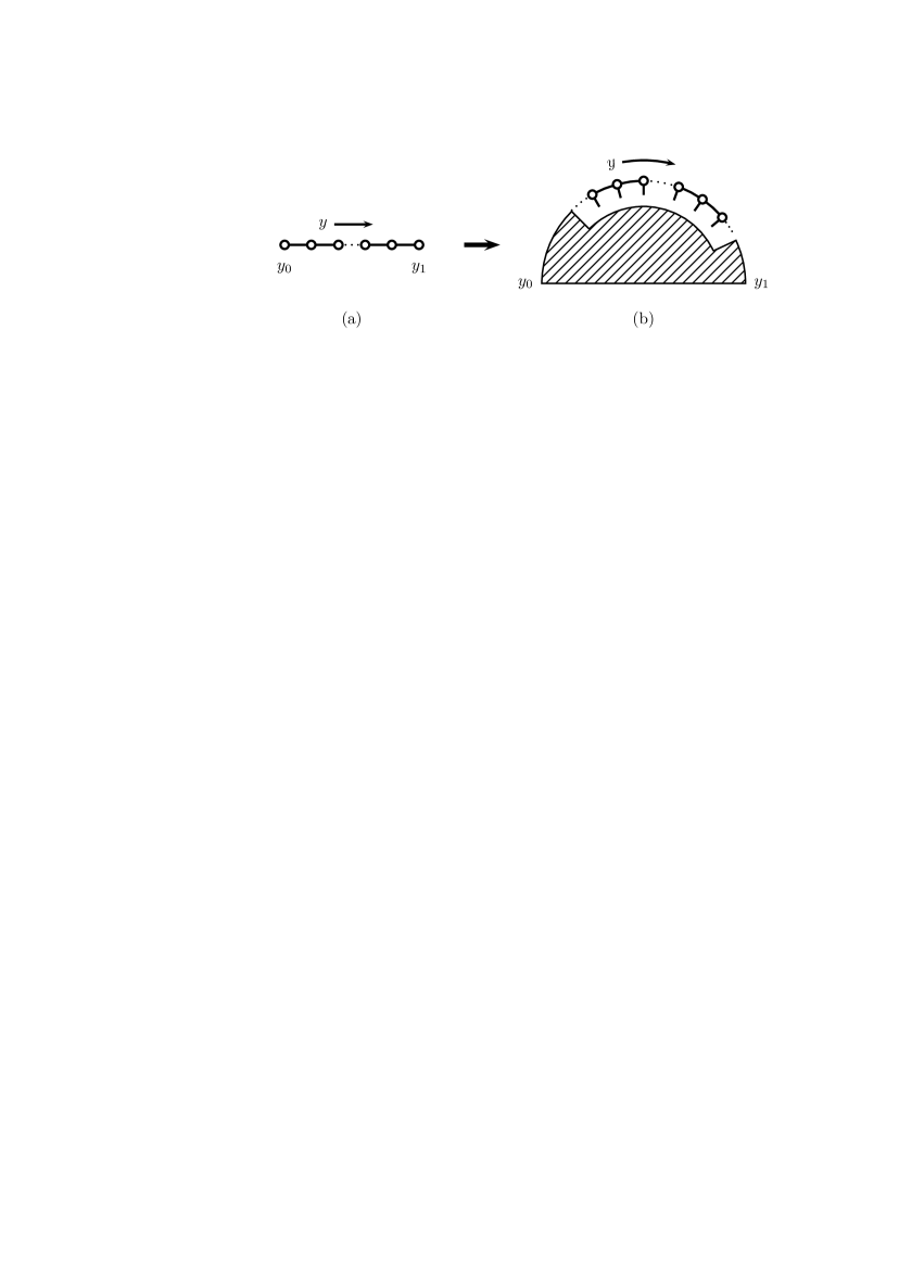
Figure 10: Comparison of a discretized gravitational 5th dimension (a) with the discrete 5D subspace on the boundary of the hyperbolic disk (b). Figure (b) shows the graph (a) wrapping the hyperbolic disk as a boundary of the fine-grained model (depicted is only a part of the discrete boundary, and the hatched region represents the remaining sites and links of the discretized disk).

This is a result of the fact that the boundary sites in graph (b) are – different from the sites of the graph (a) – also connected by radial links to the interior of the disk. Let us investigate this more explicitly for the case where the 5D spaces in Fig. 10 exhibit a non-trivial warp-factor in $y$ direction.

The geometry of the hyperbolic disk that we are interested in has both a radial dependence of the warp factor as well as a non-zero warping in $\varphi$ direction. In other words, in the language of Sec. 2, the metric is as in Eq. (1) with a new warp factor $e^{2\sigma(r,\varphi)}$, where

$$\sigma(r,\varphi)=-w\cdot r\big{(}1-\frac{\varphi}{\pi}\big{)}.$$ (57)

As before, the proper radius of the hyperbolic disk is $L$. Different from earlier, we have now a single IR brane at $(r,\varphi)=(L,0)$ and a set of UV branes that are located on a straight line extending in $\varphi=\pi$ direction from the center to the point $(L,\pi)$ on the boundary. The SM with the observer is assumed to reside on the boundary at the IR brane.

We define the common 5D geometry of the interval and the boundary in Figs. 10 (a) and (b) by restricting the coordinates on the disk to the 5D boundary sub-manifold according to $(r,\varphi)\rightarrow(L,\varphi)$. The 5D background metric is given by

$$\textrm{d}s^{2}=e^{2\sigma(y)}g_{\mu\nu}(x)\textrm{d}x^{\mu}\textrm{d}x^{\nu}-\textrm{d}y^{2},$$ (58)

where $\sigma(y)=-wvLy/[\pi\,\text{sinh}(vL)]$ and $y$ is the 5D coordinate. In terms of the disk parameters, we have $y=y(\varphi)=(\pi-\varphi)v^{-1}\text{sinh}(vL)$, i.e., $y$ is equal to the proper distance measured along the boundary between the point $(L,\varphi)$ and the UV brane at $(L,\pi)$. In Figs. 10 (a) and (b) it is $y_{0}=y(\pi)$ and $y_{1}=y(0)$.

We discretize the hyperbolic disk and use the same notation exactly as described in Secs. 5.1 and 5.2. In the discretized model, the warping in $\varphi$ direction is implemented by redefining in Eqs. (35) and (36) the quantity $\epsilon^{k}$ as $\epsilon^{k}\rightarrow\epsilon^{k}\epsilon^{-k\cdot i/N_{k}}$, where $i$ labels the $i$th site on the $k$th circle. For example, the local Planck scale on a site $(k,i)$ is now $M_{k,i}\equiv M_{4}\epsilon^{k(1-i/N_{k})}$, and the canonically normalized fields are $\hat{h}^{k,i}_{\mu\nu}=M_{4}\epsilon^{k(1-i/N_{k})}h^{k,i}_{\mu\nu}$. In the rough, local flat space approximation of Sec. 5.2, we then obtain for the mass matrix element between two fields $\hat{h}^{k,i}_{\mu\nu}$ and $\hat{h}^{l,j}_{\mu\nu}$ in the limit $N_{k}\gg 1$ the expression

$$M_{(k,i)(l,j)}\approx\frac{1}{a_{r}^{2}}\epsilon^{2(l+1)(1-i/N_{k})}[(2+\epsilon^{-2})\delta_{k,l}\delta_{i,j}-\delta_{k+1,l}(\delta_{n_{i},j}+\delta_{n_{i}+1,j})-\delta_{k-1,l}\delta_{\lceil i/2\rceil,j}],$$ (59)

where $k>0$. Again, for $\epsilon\cdot\ell\ll 1$ (e.g., $\epsilon\cdot\ell\lesssim 0.5$), the usual 4D Planck scale $M_{\text{Pl}}\approx 10^{18}\text{GeV}$ is set by the local Planck scale $M_{4}$ on the UV branes, and we have $M_{\text{Pl}}\approx M_{4}$. In general, since the UV branes are spread out on the disk around the straight line connecting the center with the point $(L,\pi)$ on the boundary, the fundamental scale $M_{4}$ will be reduced a little by a volume suppression factor; but this effect is small and can be neglected in the regime $k_{\text{max}}\simeq 10-10^{2}$, where $M_{4}$ becomes suppressed by only one or two orders of magnitude.

Switching on a non-trivial warp factor in $\varphi$ direction will practically not change $\Lambda^{6D}_{\text{bound}}$ in Eq. (56), since, for a large hyperbolic curvature of the disk, the strong coupling scale on the boundary is virtually insensitive to the circumference of the disk. Let us next compare the observed strong coupling scales for the two graphs (a) and (b) in Fig. 10: Graph (b) exhibits at the IR brane the local strong coupling scale $\Lambda^{6D}_{\text{bound}}$ given in Eq. (56). In contrast to this, we find after discretization of the 5D background in Eq. (58) that the strong coupling scale for an observer localized on the IR brane of the discretized interval in graph (a) at $y=y_{1}$ is given by

$$\Lambda^{5D}_{\text{warp}}=(wvL)^{1/2}[\pi M_{4}\,\text{sinh}(vL)]^{-1/2}(M_{k}m_{\ast}^{4}\epsilon^{4k})^{1/5},$$ (60)

where $k=k_{\text{max}}$. Thus, for large $vL$, the strong coupling scale $\Lambda^{5D}_{\text{warp}}$ in Eq. (60) drops below $\Lambda^{6D}_{\text{bound}}$ in Eq. (56). This means that the observed local strong coupling scale of 5D lattice gravity can be increased by wrapping the discretized 5th dimension around a hyperbolic disk. This requires, however, that the warping in $y$ direction is not too large: If $vL\sim 1$, then $\Lambda^{6D}_{\text{bound}}$ and $\Lambda^{5D}_{\text{warp}}$ in Eq. (60) will become identical.

Let us estimate the 5D curvature scales $-\sigma(y)/y$ for which $\Lambda^{6D}_{\text{bound}}$ becomes significantly larger than $\Lambda^{5D}_{\text{warp}}$ in Eq. (60). We consider the specific example given at the end of Sec. 5.2, where we formally take $\epsilon=(0.1)^{1/20}$ and $\ell=\ell^{1/20}$. Here, the proper radius is $k_{\text{max}}\simeq\mathcal{O}(10^{2})$ units $M_{4}^{-1}$ wide and $m_{\ast}\simeq M_{4}$. The 6D curvature scale is $w=M_{\text{Pl}}/10$ and $M_{4}\approx M_{\text{Pl}}$. On the boundary, the number of sites is $N_{k_{\text{max}}}\simeq\mathcal{O}(10^{4})$, and the local Planck scale at the IR brane is $M_{k_{\text{max}}}=\epsilon^{k_{\text{max}}}M_{\text{Pl}}\simeq 1\,\text{TeV}$. The curvature scale for the warping in $y$ direction is $-\sigma(y)/y\simeq 10^{-3}\times w$, and the strong coupling scale $\Lambda^{5D}_{\text{warp}}$ in Eq. (60) is by a factor $\sim 100$ smaller than $\Lambda^{6D}_{\text{bound}}$ in Eq. (56). We thus find that the strong coupling scale seen by an observer located on the 5D boundary sub-manifold of the disk can be significantly larger than the strong coupling scale in the corresponding discretized 5D warped space for values $-\sigma(y)/y\lesssim M_{4}\times 10^{-3}$ of the 5D curvature scale.

6 Application to Dirac neutrino masses

So far, we have only been considering the case where gravity is propagating on the disk. In this section, we will be concerned with matter in the bulk and formulate a model for small Dirac neutrino masses by implementing on the hyperbolic disk a discretized version of the volume suppression mechanism of Ref. [29]. The volume suppression mechanism in the large extra dimensional scenario is attractive, since it yields a purely geometric origin of neutrino masses. For simplicity, we shall restrict here to the coarse-grained model described in Secs. 3 and 4. Note that, in the following, gravity is not really relevant for generating neutrino masses, and we could equally well have non-gravitational extra dimensions and couple matter only to a single copy of gravity. We work, nevertheless, in the theory space of Sec. 3, since it allows to avoid the experimental bounds on extra KK-neutrinos and KK-gravitons for the same reason: The curvature of the disk generates a big mass gap between the zero mode and the higher KK-excitations that is not related to the large bulk volume.

The parent continuum theory which we discretize contains a massless right-handed (RH) SM singlet bulk neutrino that can propagate on the disk, or some sub-space thereof, while the SM fields are all located on a single point on the disk. Specifically, we consider the total action of the bulk neutrino on the disk as a combination of the following two limiting cases: (i) the bulk neutrino propagates only within the star sub-geometry of the disk and (ii) the bulk neutrino propagates only in the circle sub-geometry.

Let us first consider case (i): the action for the gravitons is described by $\mathcal{S}_{\rm disk}$ in Sec. 4.3, but the latticized RH bulk neutrino propagates only in the star sub-geometry. The bulk neutrino is represented in the discretized theory by putting on each site $i$ one 4D RH SM singlet Dirac fermion $\Psi_{i}=(\nu_{iR},\overline{\nu^{c}_{iR}})$, where $\nu_{iR}$ and $\nu_{iR}^{c}$ are 4D two-component Weyl spinors and $i=0,1,\dots,N$. The star sub-geometry, with $N$ sites surrounding the center, can be thought as being composed of $N$ two-site models that are glued together at the site $i=0$. It is convenient to label these two-site models as $(0,i)$, where $i=1,2,\dots,N$. To obtain here the action of the RH bulk neutrino, we consider each two-site model $(0,i)$ as the coarse-grained limit of a latticized fifth dimension that is compactified on an interval $[0,R_{i}]$ and apply discretized orbifold boundary conditions at the endpoints. In this picture, the continuum limit of the star sub-geometry is a configuration of $N$ continuous intervals $[0,R_{i}]$ which intersect in their common endpoint 0. The RH bulk neutrino propagates in this continuum theory as a 5D field on the intervals and is subject to orbifold boundary conditions at the endpoints of the segments $[0,R_{i}]$. We denote the 5D bulk neutrino by $\Psi=(\nu_{R},\overline{\nu^{c}_{R}})$, where $\nu_{R}$ and $\nu^{c}_{R}$ are 5D two-component Weyl spinors, and assume on each of the $N$ intervals the Neumann and Dirichlet boundary conditions $\left.(\partial\nu_{R}/\partial y_{i})\right|_{y_{i}=0,R_{i}}=0$ and $\left.\nu^{c}_{R}\right|_{y_{i}=0,R_{i}}=0$, where $y_{i}\in[0,R_{i}]$ is the coordinate of the interval $[0,R_{i}]$ and $i=1,2,\dots,N$. The discretization of these boundary conditions has been described in Refs. [11, 15, 30] and produces, in the limit where each interval $[0,R_{i}]$ is replaced by a two-site model $(0,i)$, from the latticized kinetic term of $\Psi$ the neutrino mass terms

$$\mathcal{L}_{(0,i)}=m_{\ast}(\nu_{iR}\nu^{c}_{iR}-\nu_{0R}\nu^{c}_{iR})+{\rm h.c.},$$ (61)

where we have chosen a common length $R_{i}\equiv R\sim m_{\ast}^{-1}$ for all intervals. In the flat limit $g_{\mu\nu}\rightarrow\eta_{\mu\nu}$, we then take the total action for the bulk neutrino in the star sub-geometry $\mathcal{S}_{\rm star}^{\Psi}$ to be $\mathcal{S}_{\rm star}^{\Psi}=\int{\rm d}^{4}x(\sum_{i=0}^{N}{\rm i}\overline{\Psi}_{i}\cancel{\partial}\Psi_{i}+\sum_{i=1}^{N}\mathcal{L}_{(0,i)})$. To include the effect from the boundary, let us next consider case (ii): the latticized RH bulk neutrino propagates only on the boundary of the disk. For this case, we take the action of the latticized RH neutrino on the circle $\mathcal{S}_{\rm circle}^{\Psi}$ to be of the Wilson-Dirac form $\mathcal{S}_{\rm circle}^{\Psi}=\int\textrm{d}^{4}x\sum_{i=1}^{N}({\rm i}\overline{\Psi}_{i}\,\cancel{\partial}\,\Psi_{i}+\mathcal{L}_{(i,i+1)})$, where we have introduced a discretized kinetic term

$$\mathcal{L}_{(i,i+1)}=m\cdot\nu_{iR}(\nu^{c}_{(i+1)R}-\nu^{c}_{iR})+{\rm h.c.},$$ (62)

for each pair of sites $(i,i+1)$ on the boundary of the disk. For definiteness, we suppose also that $N$ is even. The action $\mathcal{S}_{\rm circle}^{\Psi}$ has been widely discussed in the literature as a standard example for a fermion propagating in a latticized fifth dimension compactified on the circle $S^{1}$ [11] (see also, e.g., Refs. [21, 22]). Now, we define the total action of the bulk neutrino on the disk $\mathcal{S}_{\rm disk}^{\Psi}$ by simply adding the mass terms $\mathcal{L}_{(i,i+1)}$ to $\mathcal{S}_{\rm star}^{\Psi}$ such that

$$\mathcal{S}_{\rm disk}^{\Psi}=\int{\rm d}^{4}x\big{(}\sum_{i=0}^{N}\overline{\textrm{i}\Psi}_{i}\cancel{\partial}\Psi_{i}+\sum_{i=1}^{N}[\mathcal{L}_{(0,i)}+C\cdot\mathcal{L}_{(i,i+1)}]\big{)},$$ (63)

where $C$ is some suitable dimensionless parameter. The mass terms in Eq. (63) give rise to the $(N+1)\times(N+1)$ Dirac neutrino mass matrix

$$M_{D}=m_{\ast}\left(\begin{matrix}0&-1&-1&-1&\cdots&-1\\ 0&1&0&0&\cdots&0\\ 0&0&1&0&\cdots&0\\ 0&0&0&1&\ddots&\vdots\\ \vdots&\vdots&\vdots&\ddots&\ddots&0\\ 0&0&0&\cdots&0&1\end{matrix}\right)-Cm\left(\begin{matrix}0&0&0&0&\cdots&0\\ 0&-1&1&0&\dots&0\\ 0&0&-1&1&\ddots&\vdots\\ \vdots&\vdots&0&\ddots&\ddots&0\\ 0&0&\vdots&\ddots&-1&1\\ 0&1&0&\dots&0&-1\\ \end{matrix}\right),$$ (64)

where the rows and columns are spanned by $(\nu_{0R},\nu_{1R},\dots,\nu_{NR})$ and $(\nu^{c}_{0R},\nu^{c}_{1R},\dots,\nu^{c}_{NR})$, respectively. We can choose the parameter $C$ such that the matrix $M_{D}M_{D}^{\dagger}$ becomes identical with the graviton mass matrix $M_{g}^{2}$ in Eq. (14), in which case the RH neutrino masses are given by Eq. (15). The mass matrix $M_{D}M_{D}^{\dagger}$ is then diagonalized by expanding

$$\nu_{0R} = \frac{1}{\sqrt{N+1}}\hat{\nu}_{0R}-\frac{N}{\sqrt{N(N+1)}}\hat{\nu}_{NR},$$ (65a)

$$\nu_{iR} = \frac{1}{\sqrt{N}}\sum_{n=1}^{N-1}e^{-{\rm i}2\pi i\cdot n/N}\hat{\nu}_{nR}+\frac{1}{\sqrt{N+1}}\hat{\nu}_{0R}+\frac{1}{\sqrt{N(N+1)}}\hat{\nu}_{NR},$$ (65b)

where $i=1,2,\dots,N$ and $\hat{\nu}_{nR}$ ($n=0,1,\dots,N$) is the $n$th mass eigenstate belonging to the mass eigenvalue $M_{n}^{2}$ given in Eq. (15). In Eqs. (65), we thus have one zero mode neutrino $\hat{\nu}_{0R}$ with flat profile, one heavy neutrino $\hat{\nu}_{NR}$ with mass $M_{N}\sim m_{\ast}\sqrt{N}$, and $N-1$ states $\hat{\nu}_{1R},\hat{\nu}_{2R},\dots,\hat{\nu}_{N-1}$ with masses $M_{n}$ that become $M_{n}\approx m_{\ast}$, for $m_{*}\gg m$.

Let us now introduce the SM neutrinos by adding all SM fields on a single site on the boundary, e.g., on the site $i=1$. To simplify the discussion, we assume like in Ref. [29] that $B-L$ is conserved in the bulk and assign the bulk neutrino a $B-L$ number opposite to that of the SM leptons. On the site $i=1$, we then have a local Yukawa interaction $\mathcal{L}_{\rm int}=f_{\alpha}\ell_{\alpha}\textrm{i}\sigma_{2}H\nu_{1R}+\textrm{h.c.}$, where $\ell_{\alpha}=(\nu_{\alpha},\>e_{\alpha})^{T}$ are the lepton doublets with generation index $\alpha=1,2,3$, while $H$ is the Higgs doublet, and $f_{\alpha}$ is a dimensionless order one Yukawa coupling. Going to momentum basis, $\mathcal{L}_{\textrm{int}}$ approximately reads

$$\mathcal{L}_{\rm int}\approx f_{\alpha}\frac{\langle H\rangle}{\sqrt{N}}\nu_{\alpha}\hat{\nu}_{0R}+\textrm{h.c.}$$ (66)

and produces a Dirac neutrino mass term between the active neutrinos $\nu_{\alpha}$ and the zero mode $\hat{\nu}_{0R}$ that is suppressed by a volume factor $\sqrt{N}=\sqrt{Rm}$. This is the analog of the volume suppression mechanism in Ref. [29]. In the coarse-grained model, for $m_{\ast}\sim m$ and $x\equiv v/m_{\ast}\gtrsim 1$, we have $N\simeq\pi\,\textrm{exp}(x-\textrm{ln}\,x)$, i.e., a moderately large curvature $v$ [e.g., $v/m_{*}=\mathcal{O}(10)$] gives an exponentially large number of sites $N$. For $\langle H\rangle\simeq 10^{2}\>{\rm GeV}$ and $N\simeq 10^{24}$ sites, the Dirac neutrino masses will be of the right order $\sim 10^{-2}\>{\rm eV}$, which would correspond to $v/m_{\ast}\simeq 60$ in the above approximation. The important point is here that the strong coupling scale is, even in the large $N$ (or large volume) limit, always bounded from below by $\Lambda_{\textrm{disk}}=(M_{\textrm{Pl}}m_{\ast}^{4})^{1/5}$. Since all massive neutrino singlets have a mass larger than $m_{\ast}$, it follows that for $m_{\ast}\gtrsim 1\>{\rm GeV}$ all constraints on KK neutrinos from astrophysics and the early universe [31] are avoided.

Note that we have been using here the coarse-grained model with many sites on the boundary as a tool for estimating quickly the effect of putting a RH neutrino in the bulk with large volume. The number of sites $N$ measures the size of the hyperbolic disk in the corresponding continuum theory, where the same $N$ would be simply interpreted as the number of KK modes below the fundamental Planck scale. Therefore, Eq. (66) is exactly on the same footing as the well-known continuum result of Ref. [29], and provides an attractive origin for small Dirac neutrino masses.

7 Summary and Conclusions

In this paper, we have investigated gravity in a 6D geometry, where the two extra dimensions are discretized and form a hyperbolic disk with constant curvature. We have studied two types of discretizations of the disk. In our first model, we have considered a coarse-grained discretization with $N$ sites on the boundary and one site in the center of the disk. For this case, we have determined the mass spectrum and mass eigenstates of the gravitons and found in the limit of large curvature a typical KK-type spectrum sitting on top of a large mass gap between the zero mode and the first massive mode. This mass gap is set by the inverse radius of the disk while the other modes become essentially degenerate in mass. This feature allows to avoid all existing constraints on KK gravitons from Cavendish-type experiments, astrophysics, and cosmology. Additionally, this model contains a single massive mode that becomes very heavy in the large $N$ limit. We have also discussed collider signatures of the coarse-grained model at the LHC and at a possible future linear collider.

The strong coupling scale in this coarse-grained model without couplings to matter converges for large $N$ to a value like in the theory of a single massive graviton, where the graviton has a mass of the order of the inverse proper radius of the disk. This is completely different from a discrete gravitational extra dimension in 5D flat space, which exhibits a UV/IR connection problem, where the strong coupling scale would eventually go to zero when taking the large $N$ limit. This UV/IR connection problem, however, is absent in the coarse-grained model, where a sensible EFT is defined in the large $N$ limit. Even if interactions with matter are included, the theory remains valid, but with a lowered strong coupling scale. In this model, we have also studied an implementation of a bulk fermion that allows to generate small Dirac neutrino masses in the limit of a large curvature of the disk via a discrete version of the well-known volume suppression mechanism for Dirac neutrino masses in flat extra dimensions. Again, due to the particular form of the spectrum, all experimental and observational constraints on the massive KK-type neutrinos are avoided.

In our second model, we describe a fine-grained discretization of the hyperbolic disk with nonzero warping along in radial and angular direction. In this setup, the sites are situated on equidistant concentric circles and, as a result of the curvature of the disk, the number of sites on the circles grows exponentially in radial direction. We have calculated the graviton mass eigenvalues and mass eigenstates in the fine-grained model by going, as suggested previously in an analysis of the discretized 5D RS model, to a rough, local flat space approximation. Moreover, we have determined in the fine-grained model a local strong coupling scale from the kinetic mixing matrix between the gravitons and scalar Goldstones. The existence of a local strong coupling scale in the fine-grained model is, like in the corresponding 5D case, a result of the warping, which avoids the UV/IR connection problem from flat space by locally introducing an effective size or volume of the extra dimensions. Taking the coupling to matter into account, we find that the local strong coupling scale seen by a brane-localized observer on the boundary can become as large as in a discretized 5D warped model which has the background geometry of a geodesic line connecting the center with the boundary. Moreover, it turns out that the observed strong coupling behavior of gravity in discretized 5D warped space can be improved in six dimensions by wrapping the graph of the fifth dimension as a boundary around the fine-grained model. This holds for a 5D curvature scale that is roughly at least by a factor $10^{-3}$ smaller than the fundamental scale.

In conclusion, we have seen for different implementations of two discrete gravitational extra dimensions compactified on a hyperbolic disk that a high curvature or strong warping of the disk allows to avoid the UV/IR connection problem of lattice gravity in flat space. This observation is similar to the result in 5D warped space. By going to six dimensions on the hyperbolic disk, however, it is, for a range of 5D curvature scales, possible to further improve on the boundary the strong coupling behavior of lattice gravity in 5D warped space. Moreover, a strong curvature of the disk allows to avoid all constraints on KK-states and can, e.g., be employed for generating small Dirac neutrino masses in agreement with experiment.

It would be interesting to relate our analysis, e.g., also to moduli stabilization in effective theories, to theories with spontaneously broken space-time symmetries [32], and to studies on the implications of latticized extra dimensions for cosmology [33].

Appendix A Gravitational action on the hyperbolic disk

In this section, we determine the gravitational action on the hyperbolic disk $K_{2}$ introduced in Sec. 2. We start with the 6D metric $\tilde{g}_{MN}$ as defined in Eq. (1), where $\tilde{g}_{\mu\nu}=e^{2\sigma(r)}g_{\mu\nu}$, $\tilde{g}_{55}=-1$, and $\tilde{g}_{66}=-\textrm{sinh}^{2}(vr)/(v^{2})$. Partial and covariant derivatives are denoted by commas and semicolons, respectively. In these coordinates, the nonzero Christoffel symbols are given by

$$\Gamma_{\mu\nu}^{\sigma} = \frac{1}{2}\tilde{g}^{\sigma\rho}(\tilde{g}_{\mu\rho,\nu}+\tilde{g}_{\rho\nu,\mu}-\tilde{g}_{\mu\nu,\rho}),$$

$$\Gamma_{\nu 5}^{\mu} = \frac{1}{2}\tilde{g}^{\mu\rho}\tilde{g}_{\nu\rho,5},\quad\Gamma_{\nu 6}^{\mu}\>=\>\frac{1}{2}\tilde{g}^{\mu\rho}\tilde{g}_{\nu\rho,6},\quad\Gamma_{\mu\nu}^{5}\>=\>-\frac{1}{2}\tilde{g}^{55}\tilde{g}_{\mu\nu,5},\quad\Gamma_{\mu\nu}^{6}\>=\>-\frac{1}{2}\tilde{g}^{66}\tilde{g}_{\mu\nu,6},$$

$$\Gamma_{66}^{5} = -\frac{1}{2}\tilde{g}^{55}\tilde{g}_{66,5}\>=\>-\frac{1}{2v}\,\textrm{sinh}\,(2vr),\quad\Gamma_{56}^{6}\>=\>\frac{1}{2}\tilde{g}^{66}\tilde{g}_{66,5}\>=\>v\,\textrm{coth}(vr),$$ (67)

where $\Gamma^{A}_{BC}=\Gamma^{A}_{CB}$. Note that, due to the block-diagonal form of the metric $\tilde{g}_{MN}$, the internal summation in $\Gamma^{\sigma}_{\mu\nu}$ runs only over 4D indices. The 6D Ricci tensor is defined by $\tilde{R}_{MN}=\Gamma_{MA,N}^{A}-\Gamma_{MN,A}^{A}+\Gamma_{BN}^{A}\Gamma_{MA}^{B}-\Gamma_{MN}^{B}\Gamma_{BA}^{A}$, and the 6D Ricci scalar is $\tilde{R}=\tilde{R}_{MN}\tilde{g}^{MN}$. For our considerations, it is useful to introduce the quantity

$$\tilde{R}_{\rm 4D}=\tilde{g}^{\mu\nu}\big{[}\Gamma_{\mu\alpha,\nu}^{\alpha}-\Gamma_{\mu\nu,\alpha}^{\alpha}+\Gamma_{\beta\nu}^{\alpha}\Gamma_{\mu\alpha}^{\beta}-\Gamma_{\mu\nu}^{\beta}\Gamma_{\beta\alpha}^{\alpha}\big{]}.$$ (68)

Since the warp factor is only a function of $r$, we have $\Gamma_{\mu\nu}^{\sigma}=\frac{1}{2}g^{\sigma\rho}(g_{\mu\rho,\nu}+g_{\rho\nu,\mu}-g_{\mu\nu,\rho})$, and the 4D Ricci scalar $R_{\rm 4D}$ in Eq. (7) is thus related to $\tilde{R}_{\rm 4D}$ by $R_{\rm 4D}=e^{2\sigma(r)}\tilde{R}_{\rm 4D}$. In Eq. (6), we can write $\sqrt{|\tilde{g}|}\tilde{R}=\sqrt{|\tilde{g}|}(\tilde{g}^{\mu\nu}\tilde{R}_{\mu\nu}+\tilde{g}^{55}\tilde{R}_{55}+\tilde{g}^{66}\tilde{R}_{66})$, where the first term reads

$$\sqrt{|\tilde{g}|}\tilde{g}^{\mu\nu}\tilde{R}_{\mu\nu} = \sqrt{|\tilde{g}|}\tilde{g}^{\mu\nu}\big{[}\Gamma_{\mu\alpha,\nu}^{\alpha}-\Gamma_{\mu\nu,\alpha}^{\alpha}+\Gamma_{\beta\nu}^{\alpha}\Gamma_{\mu\alpha}^{\beta}-\Gamma_{\mu\nu}^{\beta}\Gamma_{\beta\alpha}^{\alpha}$$

$$- \Gamma_{\mu\nu,5}^{5}+\Gamma_{\beta\nu}^{5}\Gamma_{\mu 5}^{\beta}+\Gamma_{5\nu}^{\alpha}\Gamma_{\mu\alpha}^{5}-\Gamma_{\mu\nu}^{5}\Gamma_{5A}^{A}-\Gamma_{\mu\nu,6}^{6}+\Gamma_{\beta\nu}^{6}\Gamma_{\mu 6}^{\beta}+\Gamma_{6\nu}^{\alpha}\Gamma_{\mu\alpha}^{6}-\Gamma_{\mu\nu}^{6}\Gamma_{6A}^{A}\big{]}.$$

Here, the derivative of the Christoffel symbol with respect to $r$ (or $\varphi$) can be written as

$$-\sqrt{|\tilde{g}|}\tilde{g}^{\mu\nu}\Gamma_{\mu\nu,5}^{5}=-\left[\sqrt{|\tilde{g}|}\tilde{g}^{\mu\nu}\Gamma_{\mu\nu}^{5}\right]_{,5}+\sqrt{|\tilde{g}|}\tilde{g}^{\mu\nu}\Gamma_{A5}^{A}\Gamma_{\mu\nu}^{5}-2\sqrt{|\tilde{g}|}\tilde{g}^{\mu\alpha}\Gamma_{\alpha 5}^{\nu}\Gamma_{\mu\nu}^{5},$$ (70)

where we have used the identities $(\sqrt{|\tilde{g}|})_{,A}=\sqrt{|\tilde{g}|}\Gamma_{BA}^{B}$ and ${\tilde{g}^{\mu\nu}}_{\,\,\,\,\,\,,5}=-\tilde{g}^{\mu\alpha}\tilde{g}^{\nu\beta}\tilde{g}_{\alpha\beta,5}=-2\tilde{g}^{\mu\alpha}\Gamma_{\alpha 5}^{\nu}$ to obtain respectively the second and the third term on the right-hand side in Eq. (70). We thus have

$$\sqrt{|\tilde{g}|}\tilde{g}^{\mu\nu}\tilde{R}_{\mu\nu}=\sqrt{|\tilde{g}|}\tilde{R}_{\rm 4D}-\left[\sqrt{|\tilde{g}|}\tilde{g}^{\mu\nu}\Gamma_{\mu\nu}^{5}\right]_{,5}-\left[\sqrt{|\tilde{g}|}\tilde{g}^{\mu\nu}\Gamma_{\mu\nu}^{6}\right]_{,6}.$$ (71)

Similarly, one finds

$$\sqrt{|\tilde{g}|}\tilde{g}^{55}\tilde{R}_{55} = \left[\sqrt{|\tilde{g}|}\tilde{g}^{55}\Gamma_{A5}^{A}\right]_{,5}-\left[\sqrt{|\tilde{g}|}\tilde{g}^{55}\Gamma_{55}^{A}\right]_{,A}$$ (72a)

$$+ \sqrt{|\tilde{g}|}\tilde{g}^{55}[\Gamma_{\beta 5}^{\alpha}\Gamma_{\alpha 5}^{\beta}-\Gamma_{\alpha 5}^{\alpha}\Gamma_{\beta 5}^{\beta}-2\Gamma_{\alpha 5}^{\alpha}\Gamma_{65}^{6}],$$

$$\sqrt{|\tilde{g}|}\tilde{g}^{66}\tilde{R}_{66}\ = \left[\sqrt{|\tilde{g}|}\tilde{g}^{66}\Gamma_{A6}^{A}\right]_{,6}-\left[\sqrt{|\tilde{g}|}\tilde{g}^{66}\Gamma_{66}^{A}\right]_{,A}+\sqrt{|\tilde{g}|}\tilde{g}^{66}[\Gamma_{\beta 6}^{\alpha}\Gamma_{\alpha 6}^{\beta}-\Gamma_{\alpha 6}^{\alpha}\Gamma_{\beta 6}^{\beta}].$$ (72b)

In Eqs. (72), we have

$$\sum_{B=5,6}\Big{(}\left[\sqrt{|\tilde{g}|}\tilde{g}^{BB}\Gamma_{AB}^{A}\right]_{,B}-\left[\sqrt{|\tilde{g}|}\tilde{g}^{BB}\Gamma_{BB}^{A}\right]_{,A}-\left[\sqrt{|\tilde{g}|}\tilde{g}^{\mu\nu}\Gamma_{\mu\nu}^{B}\right]_{,B}\Big{)}$$

$$= \left[\sqrt{|\tilde{g}|}(-\tilde{g}^{\mu\nu}\Gamma_{\mu\nu}^{6}+\tilde{g}^{66}\Gamma_{\alpha 6}^{\alpha})\right]_{,6}+\left[\sqrt{|\tilde{g}|}(-\tilde{g}^{\mu\nu}\Gamma_{\mu\nu}^{5}+\tilde{g}^{55}\Gamma_{\alpha 5}^{\alpha}-\tilde{g}^{66}\Gamma_{66}^{5}+\tilde{g}^{55}\Gamma_{65}^{6})\right]_{,5},$$

and in Eq. (A) the last two terms can be written as

$$\left[\sqrt{|\tilde{g}|}(-\tilde{g}^{66}\Gamma_{66}^{5}+\tilde{g}^{55}\Gamma_{65}^{6})\right]_{,5}=2\sqrt{|\tilde{g}|}\tilde{g}^{55}\Gamma_{\alpha 5}^{\alpha}\Gamma_{65}^{6}+2\sqrt{|\tilde{g}|}\tilde{g}^{55}((\Gamma_{65}^{6})^{2}+\Gamma_{65,5}^{6}),$$ (74)

where we have used the relation $\tilde{g}^{66}\Gamma_{66}^{5}=-\tilde{g}^{55}\Gamma_{65}^{6}$. The first term on the right-hand side in Eq. (74) cancels the term $-2\sqrt{|\tilde{g}|}\tilde{g}^{55}\Gamma_{\alpha 5}^{\alpha}\Gamma_{65}^{6}$ in Eq. (72a) while the last term yields the cosmological term $\sqrt{|\tilde{g}|}\cdot(-2v^{2})$. Putting everything together, the total action $\mathcal{S}$ in Eq. (6) can be written as $\mathcal{S}=\mathcal{S}_{\rm 4D}+\mathcal{S}_{\textrm{surface}}+\mathcal{S}_{\textrm{mass}}$, where  $\mathcal{S}_{\rm 4D}$, the surface terms $\mathcal{S}_{\textrm{surface}}$, and the action $\mathcal{S}_{\textrm{mass}}$ giving rise to the graviton mass terms, respectively read

$$\mathcal{S}_{\rm 4D} = M_{6}^{4}\int\textrm{d}^{6}x\sqrt{|\tilde{g}|}\,(\tilde{R}_{\rm 4D}-2v^{2}),$$ (75a)

$$\mathcal{S}_{\textrm{surface}} = M_{6}^{4}\int\textrm{d}^{6}x\Big{(}2\left[\sqrt{|\tilde{g}|}\tilde{g}^{55}\Gamma_{\alpha 5}^{\alpha}\right]_{,5}+2\left[\sqrt{|\tilde{g}|}\tilde{g}^{66}\Gamma_{\alpha 6}^{\alpha}\right]_{,6}\Big{)},$$ (75b)

$$\mathcal{S}_{\textrm{mass}} = M_{6}^{4}\int\textrm{d}^{6}x\sqrt{|\tilde{g}|}\Big{(}\tilde{g}^{55}[\Gamma_{\beta 5}^{\alpha}\Gamma_{\alpha 5}^{\beta}-\Gamma_{\alpha 5}^{\alpha}\Gamma_{\beta 5}^{\beta}]+\tilde{g}^{66}[\Gamma_{\beta 6}^{\alpha}\Gamma_{\alpha 6}^{\beta}-\Gamma_{\alpha 6}^{\alpha}\Gamma_{\beta 6}^{\beta}]\Big{)}.$$ (75c)

Let us first consider $\mathcal{S}_{\textrm{surface}}$, which is given by

$$\mathcal{S}_{\textrm{surface}} = M_{6}^{4}\int\textrm{d}^{4}x\int_{0}^{2\pi}\textrm{d}\varphi\int_{0}^{L}\textrm{d}r\Big{(}\left[\sqrt{|\tilde{g}|}\tilde{g}^{55}\tilde{g}^{\mu\nu}\tilde{g}_{\mu\nu,5}\right]_{,5}+\left[\sqrt{|\tilde{g}|}\tilde{g}^{66}\tilde{g}^{\mu\nu}\tilde{g}_{\mu\nu,6}\right]_{,6}\Big{)}.$$ (76)

The $\varphi$-integral over the second term vanishes for periodic boundary conditions in $\varphi$-direction and the first term yields $\mathcal{S}_{\textrm{surface}}=M_{6}^{4}\int\textrm{d}^{4}x\int_{0}^{2\pi}\textrm{d}\varphi\,[\sqrt{|\tilde{g}|}\tilde{g}^{55}\tilde{g}^{\mu\nu}\tilde{g}_{\mu\nu,5}]_{r=0}^{r=L}$, which vanishes for suitable boundary conditions at $r=0,L$. In a simplified form, $\mathcal{S}_{\rm mass}$ can be written as

$$\mathcal{S}_{\textrm{mass}}=M_{6}^{4}\int\textrm{d}^{6}x\sqrt{|\tilde{g}|}\sum_{c=5,6}\Big{[}-\frac{1}{4}\tilde{g}^{cc}\tilde{g}_{\mu\nu,c}(\tilde{g}^{\mu\nu}\tilde{g}^{\alpha\beta}-\tilde{g}^{\mu\alpha}\tilde{g}^{\nu\beta})\tilde{g}_{\alpha\beta,c}\Big{]}.$$ (77)

With $\tilde{g}_{\mu\nu}=e^{2\sigma(r)}g_{\mu\nu}$, $|\tilde{g}|=e^{8\sigma(r)}|g|$, and $R_{\rm 4D}=e^{2\sigma(r)}\tilde{R}_{\rm 4D}$, we then arrive at Eq. (7).

References

- [1] L. Randall and R. Sundrum, Phys. Rev. Lett. 83 (1999) 3370, hep-ph/9905221.
- [2] L. Randall and R. Sundrum, Phys. Rev. Lett. 83 (1999) 4690, hep-th/9906064.
- [3] N. Arkani-Hamed, S. Dimopoulos, and G.R. Dvali, Phys. Lett. B 429 (1998) 263, hep-ph/9803315; Phys. Rev. D 59 (1999) 086004, hep-ph/9807344; I. Antoniadis, N. Arkani-Hamed, S. Dimopoulos, and G.R. Dvali, Phys. Lett. B 436 (1998) 257, hep-ph/9804398.
- [4] J.M. Maldacena, Adv. Theor. Math. Phys. 2 (1998) 231 [Int. J. Theor. Phys. 38 (1999) 1113], hep-th/9711200; S.S. Gubser, I.R. Klebanov, and A.M. Polyakov, Phys. Lett. B 428 (1998) 105, hep-th/9802109; E. Witten, Adv. Theor. Math. Phys. 2 (1998) 253, hep-th/9802150; O. Aharony, S.S. Gubser, J.M. Maldacena, H. Ooguri, and Y. Oz, Phys. Rept. 323 (2000) 183, hep-th/9905111.
- [5] For a review see M. Grana, Phys. Rept. 423 (2006) 91, hep-th/0509003.
- [6] N. Arkani-Hamed, H. Georgi, and M.D. Schwartz, Annals Phys. 305 (2003) 96, hep-th/0210184.
- [7] N. Arkani-Hamed and M.D. Schwartz, Phys. Rev. D 69 (2004) 104001, hep-th/0302110.
- [8] M.D. Schwartz, Phys. Rev. D 68 (2003) 024029, hep-th/0303114.
- [9] N. Boulanger, T. Damour, L. Gualtieri and M. Henneaux, Nucl. Phys. B 597 (2001) 127, hep-th/0007220; T. Damour, I.I. Kogan and A. Papazoglou, Phys. Rev. D 66 (2002) 104025, hep-th/0206044; N. Kan and K. Shiraishi, Class. Quant. Grav. 20 (2003) 4965, gr-qc/0212113; Prog. Theor. Phys. 111 (2004) 745, gr-qc/0310055; C. Deffayet and J. Mourad, Class. Quant. Grav. 21 (2004) 1833, hep-th/0311125; G. Cognola, E. Elizalde, S. Nojiri, S. D. Odintsov and S. Zerbini, Mod. Phys. Lett. A 19 (2004) 1435, hep-th/0312269.
- [10] N. Arkani-Hamed, A.G. Cohen, and H. Georgi, Phys. Rev. Lett. 86 (2001) 4757, hep-th/0104005.
- [11] C.T. Hill, S. Pokorski, and J. Wang, Phys. Rev. D 64 (2001) 105005, hep-th/0104035.
- [12] L. Randall, M.D. Schwartz, and S. Thambyapillai, JHEP 0510 (2005) 110, hep-th/0507102.
- [13] J. Gallicchio and I. Yavin, JHEP 0306 (2006) 079, hep-th/0507105.
- [14] A. Falkowski and H.D. Kim, JHEP 0208 (2002) 052, hep-ph/0208058.
- [15] T. Bhattacharya, C. Csaki, M.R. Martin, Y. Shirman, and J. Terning, JHEP 0508 (2005) 061, hep-lat/0503011.
- [16] H.C. Cheng, C.T. Hill, and J. Wang, Phys. Rev. D 64 (2001) 095003, hep-ph/0105323; H. Abe, T. Kobayashi, N. Maru, and K. Yoshioka, Phys. Rev. D 67 (2003) 045019, hep-ph/0205344; L. Randall, Y. Shadmi, and N. Weiner, JHEP 0301 (2003) 055, hep-th/0208120; A. Katz and Y. Shadmi, JHEP 0411, 060 (2004), hep-th/0409223; C.D. Carone, J. Erlich, and B. Glover, JHEP 0510 (2005) 042, hep-ph/0509002; J. de Blas, A. Falkowski, M. Perez-Victoria, and S. Pokorski, hep-th/0605150.
-
[17]
M. Sremcević, R. Sazdanović, and S. Vukmirović,
http://library.wolfram.com/infocenter/MathSource/4540. - [18] See, e.g., G. ’t Hooft and M.J.G. Veltman, Annales Poincaré Phys. Theor. A 20 (1974) 69; M.J.G. Veltman, in Les Houches 1975: Methods in Field Theory, North-Holland, Amsterdam (1976); P. Van Nieuwenhuizen, Phys. Rept. 68 (1981) 189.
- [19] M. Fierz and W. Pauli, Proc. Roy. Soc. Lond. A 173 (1939) 211.
- [20] P. Creminelli, A. Nicolis, M. Papucci, and E. Trincherini, JHEP 0509, 003 (2005), hep-th/0505147.
- [21] F. Bauer, M. Lindner, and G. Seidl, JHEP 0405 (2004) 026, hep-th/0309200.
- [22] T. Hällgren, T. Ohlsson, and G. Seidl, JHEP 0502 (2005) 049, hep-ph/0411312.
- [23] H.D. Kim, JHEP 0601 (2006) 090, hep-th/0510229.
- [24] See, e.g., C.D. Hoyle, D.J. Kapner, B.R. Heckel, E.G. Adelberger, J.H. Gundlach, U. Schmidt, and H.E. Swanson, Phys. Rev. D 70 (2004) 042004, hep-ph/0405262.
- [25] S. Hannestad and G.G. Raffelt, Phys. Rev. Lett. 88 (2001) 071301, hep-ph/0110067.
- [26] L.J. Hall and D.R. Smith, Phys. Rev. D 60 (1999) 085008, hep-ph/9904267; S. Hannestad, Phys. Rev. D 64 (2001) 023515, hep-ph/0102290.
- [27] G.F. Giudice, R. Rattazzi, and J.D. Wells, Nucl. Phys. B 544 (1999), hep-ph/9811291.
- [28] B. Bellazzini and A. Mintchev, J. Phys. A 39 (2006) 11101, hep-th/0605036; S.A. Fulling, math.sp/0508335.
- [29] N. Arkani-Hamed, S. Dimopoulos, G.R. Dvali, and J. March-Russell, Phys. Rev. D 65 (2002) 024032, hep-ph/9811448; K.R. Dienes, E. Dudas, and T. Gherghetta, Nucl. Phys. B 557 (1999) 25, hep-ph/9811428; G.R. Dvali and A.Y. Smirnov, Nucl. Phys. B 563 (1999) 63, hep-ph/9904211.
- [30] W. Skiba and D. Smith, Phys. Rev. D 65 (2002) 095002, hep-ph/0201056.
- [31] See, e.g., R. Barbieri, P. Creminelli and A. Strumia, Nucl. Phys. B 585 (2000) 28, hep-ph/0002199, and references therein.
- [32] I. Kirsch, Phys. Rev. D 72 (2005) 024001, hep-th/0503024; N. Boulanger and I. Kirsch, Phys. Rev. D 73 (2006) 124023, hep-th/0602225.
- [33] F. Bauer and G. Seidl, Phys. Lett. B 624, 250 (2005), hep-ph/0506184; T. Hällgren and T. Ohlsson, JCAP 0606 (2006) 014, hep-ph/0510174.