Université Libre de Bruxelles
Faculté des Sciences
Service de Physique Théorique et Mathématique

Kac-Moody Algebras in M-theory

Sophie de Buyl

Aspirant F.N.R.S.

Année académique 2005–2006

Mes remerciements s’adressent tout d’abord à Marc Henneaux, mon directeur de thèse. Quand j’étais petite, ses cours sur les représentations des groupes finis et sur la Relativité Générale m’ont fortement séduite. Je garde un excellent souvenir de ses exposés d’une clarté remarquable. J’ai donc osé frapper à sa porte et c’est avec joie que j’ai entrepris un mémoire, puis la présente thèse dans le cadre de la gravitation d’Einstein, non plus sur les groupes finis, mais sur des structures beaucoup plus grandes: les algèbres de Kac–Moody infini dimensionnelles. Il m’a proposé des problèmes stimulants et bien posés me permettant d’entrer rapidement dans des sujets pointus. J’ai beaucoup apprécié sa manière positive de voir les choses, ainsi que son intuition qui —à ma connaissance— n’a jamais été mise en défaut. J’ai été impressionnée par son efficacité: dès qu’il se décide à terminer un projet, c’est comme si c’était fait! Et malgré sa présence euh… disons fort aléatoire, il a été pour moi un promoteur exemplaire. Maintenant que je suis grande, j’espère être à la hauteur de ses attentes et pouvoir voler de mes propres ailes.

Je remercie de tout coeur Christiane Schomblond. Elle a guidé mes premiers pas, parfois trop hatifs, dans le monde de la recherche scientifique et a été une source de réponses indispensable tout au long de l’élaboration de cette thèse. Je lui en suis fort reconnaissante et suis très sensible à sa grande disponibilité. C’est avec grand plaisir que j’ai travaillé avec Laurent Houart. La porte de son bureau toujours ouverte, et à deux pas de la mienne, a contribué au partage de son enthousiasme (débordant certains jours et ayant le don d’accélérer le débit de ses propos) pour les very interesting Kac–Moody algebras. Je le remercie pour son attention face à mes angoisses diverses, dont celles de parler en anglais devant des monsieurs sérieux.

Louis Paulot a été un collaborateur hors pair pour affronter le monde sans pitié des fermions et les diagrammes de Satake, je lui suis reconnaissante pour les nombreuses choses qu’il m’a apprises. Je remercie également Nassiba Tabti et Gaïa Pinardi pour des collaborations passées ainsi que Geoffrey Compère pour collaboration sur le feu… Je remercie Stéphane Detournay pour les mille et un projets qu’il m’a proposés et que je compte bien partager avec lui malgré les embûches sur notre chemin de post–doctorants.

Sandrine Cnockaert occupe certainement une place particulière dans ces remerciements. Nous avons effectivement suivi un parcours très proche (mais dans des états de stress plus ou moins opposés). Je la remercie pour plein de petites choses qui ont contribué au bon déroulement de cette thèse. Aujourd’hui nos voies semblent s’éloigner mais je suis sûre qu’elles garderont des points communs.

J’ai eu la chance de rencontrer diverses personnes qui m’ont accompagnée le long de mon parcours scientifique. Je pense ici à Philippe Léonard qui a éveillé mon intéret pour la physique. Puis à Kim Claes, Laura Lopez–Honorez, Sandrine Cnockaert, Claire Noël, Georges Champagne et Yannick Kerckx [par ordre de taille] qui ont contribué à créer une atmosphère stimulante pendant nos quatre années d’études universitaires. J’ai eu la chance de faire partie d’un service fort dynamique qui semble grandir de plus en plus. J’en remercie tous les membres, les secrétaires si efficaces, les habitués de la salle café et les doctorants (et ex–doctorant) du couloir N du 6ième étage et puis tous ceux que j’oublie. J’ai profité de l’exprérience de mes ainés, Xavier Bekaert et Nicolas Boulanger, que je tiens beaucoup à remercier. L’enthousiasme contagieux de Jarah Evslin, Daniel Persson, Carlo Maccafferi, Nazim Bouatta, Geoffrey Compère, Mauricio Leston, Stéphane Detournay et Stanislav Kuperstein [l’interpretation de l’ordre de présentation est laissée au lecteur] lors des “Weinberg lectures” dont j’ai malheureusement manqué nombre d’épisodes ainsi que le bruit qu’ils font en discutant de physique est extrêment motivant! Je leur souhaite à tous les meilleures découvertes … Pour diverses discussions, je remercie [dans un ordre aléatoire] Philippe Spindel, Glenn Barnich, François Englert, Thomas Fischbacher, Pierre Bieliavsky, Axel Kleinschmidt, Arjan Keurentjes, Riccardo Argurio et Nicolas Boulanger. Il me tient à coeur d’évoquer la première “Modave Summer School in Mathematical Physics” et tous ses participants si avides de savoir.

Etant de nature plutôt anxieuse et ne maîtrisant pas vraiment la langue de Shakespeare, j’ai beaucoup de remerciements à adresser concernant ma rédaction. Ma thèse a subi d’innom-brables améliorations suite aux lectures et re–lectures de Christiane Schomblond. Je lui suis fort reconnaissante pour sa patience, ses conseils avisés et son exigence face à mon style parfois invontairement peu clair… Je remercie vivement Marc Henneaux pour sa lecture très attentive et les précisions apportées. Daniel Persson m’a encouragée, aidée et a ponctué différentes étapes de ma rédaction de “I think this is a good job!”. Geoffrey Compère a grandement contribué à la clarté de cet exposé, je lui en suis fort reconnaissante. Je remercie également Stéphane Detournay, mon fabricant de phrases préféré, ainsi que Sandrine Cnockaert pour leur aide indispensable dans la phase finale de rédaction. Je n’oublie pas non plus ici Mauricio Leston, Louis Paulot, Laurent Houart et Paola Aliani. Finalement, je remercie le cnrs pour son dictionnaire en ligne $http://dico.isc.cnrs.fr/fr/index\_tr.html$ dont j’ai usé et abusé, je l’espère à bon escient.

Je remercie Thomas Hertog, Laurent Houart, Bernard Julia, Bernhard Mühlherr, Christiane Schomblond, Philippe Spindel et Michel Tytgat pour avoir accepté de faire partie de mon jury.

Pour les longues heures passées pendue au fil du téléphone à gémir en leur assurant que non je n’y arriverais jamais, que je n’étais un pauvre petit lapin, je remercie tout particulièrement ma maman, mon frère Pierre et Sophie Van den Broeck. Ils ont eu l’oreille plus qu’attentive à mes nombreux doutes quant au bon fonctionnement de mes neurones… Pour, lorsque j’habitais chez mes parents, avoir été d’une compréhension totale et plus tard pour avoir continué à satisfaire mes petits caprices, je remercie mon papa. Pour me rappeler que la physique peut avoir des applications pratiques et ne pas céder à mes quatre volontés, je remercie mon frère Martin. Je pense ici aussi à Aurélie Feron, Françoise de Halleux et encore à Sophie Van den Broeck dont l’amitié m’est particulièrement chère. A ma famille et mes amis: j’oublie pas que j’vous aime!

Je remercie beaucoup ma grand–mère, Grand–Mamy, pour son support informatique! Pour sa disponibilité et ses connaissances en linux, LaTeX , mathematica, maple et bugs divers et variés des nombreux ordinateurs que j’ai u(tili)sés, je remercie Pierre de Buyl. Glenn Barnich a aussi été d’une patience exemplaire lors des réinstallations de différents systèmes d’exploitation ainsi que pour divers problèmes quotidiens.

La physique mène à des choses diverses et variées ainsi qu’ à de nombreuses rencontres, je vous laisse deviner celle qui m’a comblée au-delà de toute espérance.

Introduction

One of the main challenges of contemporary physics is the unification of the four fundamental interactions. On the one hand, the electromagnetic, weak and strong interactions have been unified in the general framework of quantum field theory, within the Standard Model. This theory provides a quantum description of these interactions in agreement with special relativity but restricted to a regime where gravity can be neglected. Numerous predictions of the Standard Model have been verified with an impressive accuracy through experiments with particles colliding in accelerators. On the other hand, the gravitational interaction has a very different status since, according to Einstein’s General Relativity which remains its current best description, gravity is encoded in the curvature of spacetime induced by the presence of matter. In this context, spacetime becomes dynamical, which is different to what happens in quantum field theory where particles propagate in a fixed background. General Relativity successfully computed the perihelion precession of Mercury, the deflection of light by the sun, etc… and it is even used in our everyday life through the global positioning system. But it is a classical theory, and cannot be applied to energy scales larger than the Planck energy. In some extreme situations such as those encountered in the center of black holes or at the origin of the universe, all interactions become simultaneously relevant. Unfortunately, direct attempts to express General Relativity in quantum mechanical terms have led to a web of contradictions, basically because the non–linear mathematics necessary to describe the curvature of spacetime clashes with the delicate requirements of quantum mechanics [83]. This situation is clearly not satisfactory and a theory encompassing all fundamental interactions must be found. This hypothetic theory should reproduce the Standard Model and General Relativity in their respective domains of validity.

So far, the most promising candidate for such a unification is string theory. The basic idea of string theory is to replace the point particles by one–dimensional objects. These one–dimensional objects can vibrate and the different vibration modes correspond to various particles. A very exciting feature of string theories is that their particle spectra contain a graviton (the hypothetic particle mediating the quantum gravitational interaction) and may contain particles mediating the other three forces. String theory predicts additional spatial dimensions, and supersymmetry — mixing bosons and fermions — is a key ingredient. A drawback of string theories is that a satisfactory formulation based on first principles is still missing. Another drawback at first sight is that there exist five coherent supersymmetric string theories: type I, type IIA, type IIB, heterotic $E_{8}\times E_{8}$ and heterotic $SO(32)$. One may wonder how to choose the one which is the most fundamental? Fortunately, relations between these theories, named dualities, have been discovered during the nineties. There are essentially two types of dualities: the T–dualities and the S–dualities.

In order to understand how T–duality acts, some knowledge of dimensional reduction is necessary. If one of the space–like dimensions is assumed to take its values on a circle of radius $R$, a closed string can wrap $\omega$ times around this circle. Winding requires energy because the string must be stretched against its tension and the amount of energy is $\omega R/\ell_{st}^{2}$, where $\ell_{st}$ is the string length. This energy is quantised since $\omega$ is an integer. A string travelling around this circle has a quantised momentum around the circle; indeed, its momentum is proportional to the inverse of its wavelength $\lambda=2\pi R/n$, where $n$ is an integer. The momentum around the circle — and the contribution to its energy — goes like $n/R$. At large $R$ there are many more momentum states than winding states (for a given maximum energy), and conversely at small $R$. A theory with large $R$ and a theory with small $R$ can be equivalent, if the role of momentum modes in the first is played by the winding modes in the second, and vice versa. Such a T–duality relates type IIA superstring theory to type IIB superstring theory. This means that if we take type IIA and type IIB theories and compactify them on a circles, then switching the momentum and winding modes as well as inverting the radii, changes one theory into the other. The same is also true for the two heterotic theories.

In contrast with standard quantum field theories, the coupling constant of the string depends on a spacetime field called the dilaton. Replacing the dilaton field by minus itself exchanges a very large coupling constant for a very small one. An S–duality is a relation exchanging the strong coupling of one theory with the weak coupling of another one. If two string theories are related by S–duality, then the first theory with a strong coupling constant is the same as the other theory with a weak coupling constant. Superstring theories related by S–duality are: type I superstring theory with heterotic $SO(32)$ superstring theory, and type IIB theory with itself.

It turns out that T–duality of compactified string theories and S–duality do not commute in general but generate the discrete U–duality group [98]. In particular, when compactifying type II string theories on a $d$–torus, the conjectured U–duality group is the discrete group $E_{d+1(d+1)}({\mathbb{Z}})$.

The discovery of the various dualities between the five $D=10$ superstring theories suggested that each of them could be a part of a more fundamental theory that has been named M–theory [178]. Much of the knowledge about M–theory comes from the study of the $D=10$ maximal supergravity theories which encode the complete low energy behaviour of all the known superstring theories. Moreover, the $D=11$ supergravity [31] has been argued to be the low energy limit of M–theory [178]. This theory has a special status: it is the highest dimensional supergravity theory and it is unique in $D=11$ [139].

Although very little is known about M–theory, it is believed that M–theory should be a background independent theory that would give rise to spacetime as a secondary concept. It is expect that M–theory should also possess a rich symmetry structure. Since symmetries have always been a powerful guide in the formulation of fundamental interactions, the knowledge of the symmetry group of M–theory would certainly constitute an important step towards an understanding of its underlying structure. The following statement is therefore very intriguing: the infinite–dimensional Kac–Moody group $E_{11(11)}$ has been conjectured to be the symmetry group of M–theory [177, 126]. The corresponding Kac–Moody algebra $\mathfrak{e}_{11(11)}$ is the very extension of the finite dimensional Lie algebra $\mathfrak{e}_{8(8)}$. [ More precisely $\mathfrak{e}_{8(8)}^{+++}$ is the split real form of the complex Kac–Moody algebra $\mathfrak{e}_{8}^{+++}$ defined by the Dynkin diagram depicted in Figure 1, obtained from those of $\mathfrak{e}_{8}$ by adding three nodes to its Dynkin diagram [80]. One first adds the affine node, labelled 3 in the figure, then a second node labelled 2, connected to it by a single line and defining the overextended ${\mathfrak{g}}^{++}$ algebra, then a third one labelled 1, connected by a single line to the overextended node.]

Figure 1: The Dynkin diagram of $\mathfrak{e}_{8}^{+++}$

This conjecture is supported by the fact that evidence has been given according to which the bosonic sector of $D=11$ supergravity could be reformulated as a non–linear realisation based on the Kac–Moody group $E_{11(11)}$ and the conformal group [176, 177]. Theories of type IIA and IIB can also be reformulated as non–linear realisations based on $E_{11(11)}$ [159, 176]. The $E_{11(11)}$ group contains the Lorentz group which is evidently a symmetry of the perturbative theory but it also contains symmetries which are non–perturbative. The simplest example is provided by the case of IIB theory: the $E_{11(11)}$ symmetry contains its $SL(2,{\mathbb{R}})$ symmetry [160] which acts on the dilaton and therefore mixes perturbative with “non–perturbative” phenomena.

The relevance of infinite–dimensional Kac–Moody algebras as symmetries of gravitational theories has already been pointed in [105, 106, 103]: it has been conjectured that the dimensional reduction of $D=11$ supergravity down to one dimension would lead to the appearance of the Kac–Moody group $E_{8(8)}^{++}=E_{10(10)}$. In this context, $E_{10(10)}$ is called a hidden symmetry of $D=11$ supergravity since it was thought to appear only after dimensional reduction (and/or dualisations of certain fields). The emergence of hidden symmetries is not particular to $D=11$ supergravity: they also appear in other supergravities and in pure gravity. Their full implications are to a large extent still mysterious. Before concentrating on dimensional reduction of $D=11$ supergravity, let us recall the first example of hidden symmetries and comment about the $N=8$, $D=4$ supergravity.

This first example comes from the study of solutions of the Einstein equations of pure gravity in $D=4$ admitting Killing vectors. The Ehlers $SL(2,{\mathbb{R}})$ group is a symmetry group acting on certain solutions possessing one Killing vector [67]. When combined with the Matzner–Misner group, it leads to an infinite–dimensional symmetry — the Geroch group — acting on solutions of Einstein’s equations with two commuting Killing vectors (axisymmetric stationary solutions) [82]. The Geroch group has been identified with the affine extension of $SL(2,{\mathbb{R}})$, namely the affine Kac–Moody group $SL(2,{\mathbb{R}})^{+}$ [105]. These results also provided a direct link with the integrability of these theories in the reduction to two dimensions, i.e. the existence of Lax pairs for the corresponding equations of motion [66, 124, 17, 131, 13].

Hidden symmetries have further been discovered in various supergravities [26, 27]. The maximal $N=8$ supergravity in $D=4$ was shown to possess an $E_{7(7)}$ symmetry; the $D>4$ theories which reproduce this theory upon dimensional reduction(s) à la Kaluza–Klein also possess hidden symmetries which are displayed in Table 1. Non–maximal ($N<8$) supergravities in $D=4$ — obtained by consistent truncations of the fields decreasing the number of supersymmetries of the $N=8$ supergravity in $D=4$ — and their higher dimensional parents again exhibit hidden symmetries. [The $D=3$ theories obtained from the $D=4$ ones also give rise to hidden symmetries.] All these symmetries enter very nicely in the so–called magic triangle of Table 1. For each $N$, the highest dimensional theory is said to possess hidden symmetries since it possesses symmetries revealed only after dimensional reduction and suitable dualisations of fields.

Table 1: Real magic triangle Cosets: $N$ is the number of supersymmetries in $D=4$, $D$ the spacetime dimension and a $+$ means that a theory exists but possesses no scalars. The remarkable property of the magic triangle is its symmetry — up to the particular real form — with respect to the diagonal (see [91] for more details).

	$N=8$	$N=6$	$N=5$	$N=4$	$N=3$	$N=2$	$N=1$	$N=0$
$D=11$	$+$
$D=10$	${\mathbb{R}}$
$D=9$	${SL(2)\over SO(2)}\times{\mathbb{R}}$
$D=8$	${SL(3)\times SL(2)\over SO(3)\times SO(2)}$
$D=7$	${SL(5)\over SO(5)}$
$D=6$	${SO(5,5)\over SO(5)\times SO(5)}$	${SO(5,1)\times SO(3)\over SO(5)\times SO(3)}$
$D=5$	${E_{6(6)}\over Usp(8)}$	${SU^{\star}(6)\over Usp(6)}$
$D=4$	${E_{7(7)}\over SU(8)}$	${SO^{\star}(12)\over U(6)}$	${SU(5,1)\over U(5)}$	${SU(4)\times SU(1,1)\over SU(4)\times SO(2)}$	${U(3)\over U(3)}$	${U(2)\over U(2)}$	${U(1)\over U(1)}$	+
$D=3$	${E_{8(8)}\over Spin(16)/{\mathbb{Z}}_{2}}$	${E_{7(-5)}\over SO(12)\times SO(3)}$	${E_{6(-14)}\over SO(10)\times SO(2)}$	${SO(8,2)\over SO(8)/{\mathbb{Z}}_{2}\times SO(2)}$	${SU(4,1)\over SO(6)\times SO(2)}$	${SU(2,1)\times SU(2)\over SO(4)\times SO(2)}$	${SL(2)\times SO(2)\over SO(2)\times SO(2)}$	${SL(2)\over SO(2)}$

Let us now focus on the $D=11$ supergravity, which is of particular interest in the context of M–theory, and its successive dimensional reductions (for excellent lecture notes on the subject see [150]). More precisely, we will consider the scalar sector of the reduced theories since it can be shown that the symmetry of the scalar sector extends to the entire Lagrangian [150]. Performing successive dimensional reductions on an circle, a torus, … an $n$–torus increases the number of scalar fields. Indeed, from the $(D-1)$–dimensional point of view, the $D$–dimensional metric is interpreted as a metric, a 1–form called graviphoton and a scalar field called dilaton while a $D$–dimensional $p$–form potential yields a $p$–form potential and a $(p-1)$–form potential. The scalar fields appearing in successive dimensional reduction of the $D=11$ supergravity down to $D<11$, including those that arise from dualisation of forms, combine into a non–linear realisation of a group ${\cal G}$. More precisely, they parametrise a coset space ${\cal G}/{\cal K}$ where ${\cal K}$ is the maximally compact subgroup of ${\cal G}$, see Table 2. These results deserve some comments:

– When a gravity theory coupled to forms is reduced on an $n$–torus, one expects that the reduced Lagrangian possesses a $GL(n,{\mathbb{R}})$ symmetry since this is the symmetry group of the $n$–torus and one assumes that the reduced fields do not depend on the reduced dimensions. In the case at hand, this is what happens in $D=10$ and $D=9$. $D=8$ is the first dimension in which one gets a scalar from the reduction of the $D=11$ 3–form. The symmetry in $D=8$ is an $SL(3,{\mathbb{R}})\times SL(2,{\mathbb{R}})$ symmetry instead of the expected $GL(3,{\mathbb{R}})=SL(3,{\mathbb{R}})\times{\mathbb{R}}$ symmetry: this is because there is a congruence between the scalar field coming from the $D=11$ 3–form potential and the scalar fields arising from the reduction of the metric. The same kind of phenomenon happens in lower dimensions.

– Three–dimensional spacetimes are special because there all physical (bosonic) degrees of freedom can be converted into scalars: the scalar fields arising from the dualisation of the 1–form potential contribute to the $E_{8(8)}$ symmetry in $D=3$.

Going down bellow three dimensions, one obtains Kac–Moody extensions of the exceptional $E$–series. The two–dimensional symmetry $E_{9(9)}$ is, like the Geroch group, an affine symmetry [106, 17, 141]. In one–dimensional spacetimes, the expected symmetry is the hyperbolic extension $E_{10(10)}$ [105, 106, 103] and in zero–dimensional spacetimes, one formally finds the Lorentzian group $E_{11(11)}$.

Table 2: The symmetry groups of the $D=11$ supergravity reduced on an $n$–torus are given in this table. The scalar sector in $D=11-n$ fits into a non–linear realisation based on the coset spaces ${\cal G}/{\cal K}$ where ${\cal K}$ is the maximally compact subgroup of ${\cal G}$.

$D$	${\cal G}$	${\cal K}$
$10$	${\mathbb{R}}$	1
$9$	$SL(2,{\mathbb{R}})\times{\mathbb{R}}$	$SO(2)$
$8$	$SL(3,{\mathbb{R}})\times SL(2,{\mathbb{R}})$	$SO(3)\times SO(2)$
$7$	$SL(5,{\mathbb{R}})$	$SO(5)$
$6$	$Spin(5,5,{\mathbb{R}})$	$(Sp(2)\times Sp(2))/{\mathbb{Z}}_{2}$
$5$	$E_{6(6)}$	$Sp(4)$
$4$	$E_{7(7)}$	$SU(8)/{\mathbb{Z}}_{2}$
$3$	$E_{8(8)}$	$Spin(16)/{\mathbb{Z}}_{2}$
$2$	$E_{9(9)}$	$K(E_{9(9)})$
$1$	$E_{10(10)}$	$K(E_{10(10)})$
$0$	$E_{11(11)}$	$K(E_{11(11)})$

The hidden symmetries encompass the U–duality [146]: in the case of type II string theories compactified to $n$ dimensions on an $(11-n)$–torus the conjectured U–duality group is the discrete group $E_{11-n(11-n)}({\mathbb{Z}})$, which is a subgroup of the hidden group $E_{11-n(11-n)}$ in $D=11-n$ dimensions.

Another reason to think that infinite–dimensional Kac–Moody algebras might be symmetries of gravitational theories comes from Cosmological Billiards, which shed a new light on the work of Belinskii, Khalatnikov and Lifshitz (BKL) [10, 12, 11]. BKL gave a description of the asymptotic behaviour, near a space–like singularity, of the general solution of Einstein’s empty spacetime equations in $D=4$. They argued that, in the vicinity of a space–like singularity, the Einstein’s equations — which are a system of partial differential equations in 4 variables $(t,x_{i})$ — can be approximated by a 3–dimensional family, parametrised by $(x_{i})\in{\mathbb{R}}^{3}$, of ordinary differential equations with respect to the time variable $t$. This means that the spatial points effectively decouple. The coefficients entering the non–linear terms of these ordinary differential equations depend on the spatial point $x_{i}$ but are the same, at each given $x_{i}$, as those that arise in the Bianchi type IX or VIII spatially homogeneous models. References [118, 23, 10, 12, 11] provide a description of this general asymptotic solution in terms of chaotic successions of generalised Kasner solutions [a Kasner solution is given by a metric $ds^{2}=-dt^{2}+t^{2p^{1}}(dx^{1})^{2}+t^{2p^{2}}(dx^{2})^{2}+t^{2p^{3}}(dx^{3})^{2}$ where $p^{1},p^{2},p^{3}$ are constants subject to $p^{1}+p^{2}+p^{3}=(p^{1})^{2}+(p^{2})^{2}+(p^{3})^{2}=1$; a generalised Kasner solution can be obtained from the Kasner solution by performing a linear transformation on the metric in order to “un–diagonalise” it]. Using Hamiltonian methods, these chaotic successions have been shown to possess an interpretation in terms of a billiard motion on the Poincaré disk [24, 135].

The emergence of Kac–Moody structure à la limite BKL has given a new impulse to this field [41, 40, 39, 44]. This approach allows to tackle theories of gravity coupled to $p$–forms and dilatons in any spacetime dimensions and generalises the previous works. In reference [44] a self–consistent description of the asymptotic behaviour of all fields in the vicinity of a space–like singularity as a billiard motion is given. It is also shown how to systematically derive the billiard shape, in particular the position and orientation of the walls, from the field content and the explicit form of the Lagrangian. The striking result is that, when one studies the asymptotic dynamics of the gravitational field and the dilatons, the shape of the billiard happens to be the fundamental Weyl chamber of some Lorentzian Kac–Moody algebra for pure gravity in $D\leq 10$ as well as for all the (bosonic sector of the) low energy limits of the superstring theories and $D=11$ supergravity [40, 41, 39].

Depending on the theory under consideration, there are essentially two types of behaviours. Either the billiard volume is finite and the asymptotic dynamics is mimicked by a monotonic Kasner–like regime or the billiard volume is infinite and the asymptotic dynamics is a chaotic succession of Kasner epochs. When the billiard is associated with a Kac–Moody algebra, the criterium for the behaviour to be chaotic is that the Kac–Moody algebra be hyperbolic [42]. The spacetime dimension 10 is critical from this point of view. Indeed, it has been shown that pure gravity in $D$ dimensions is related, in this context, to the over–extended Kac–Moody algebra $A_{D-3}^{++}$. This algebra is hyperbolic for $D\leq 10$ and therefore the asymptotic dynamics are chaotic [65, 63]. The Kac–Moody algebras relevant for the (bosonic sector of the) low energy limits of various superstring theories and for the $D=11$ supergravity are also hyperbolic. Note that the $D=11$ supergravity asymptotic dynamics is chaotic in spite of the fact that $D>10$, thanks to the crucial presence of the 3–form potential.

The question arose whether the appearance of these Kac–Moody algebras in the asymptotic regime was a manifestation of the actual symmetry of the full theory. A way to tackle this question is to write an action explicitly invariant under the relevant Kac–Moody algebra and compare the equations of motion of this action with the ones of the gravitational theory. Let us specify this discussion to the bosonic sector of the $D=11$ supergravity for which the relevant Kac–Moody group is $E_{10(10)}=E_{8(8)}^{++}$. An action $S_{E_{8(8)}^{++}}$ invariant under this group can be constructed by considering a geodesic motion, depending on time, on the coset space $E_{10(10)}/K(E_{10(10)})$, where $K(E_{10(10)})$ is the maximally compact subgroup of $E_{10(10)}$ [43]. This coset space being infinite–dimensional, the motion is parametrised by an infinite number of fields and a “level” is introduced to allow a recursive approach. On the $D=11$ supergravity side, one considers a “gradient” expansion of the bosonic equations of motion. It has been shown that, up to a certain level, the level expansion and the gradient expansion match perfectly provided one adopts a dictionary mapping spacetime bosonic fields at a given spatial point to time dependent geometrical quantities entering the coset construction [43]. A key ingredient to establish this dictionary is that the level relies on the choice of a $\mathfrak{sl}(10,{\mathbb{R}})$ subalgebra of the Kac–Moody algebra $\mathfrak{e}_{10(10)}$ the representations of which can be identified with spacetime fields. Unfortunately, the Kac–Moody algebras are poorly understood and this causes problems to continue the comparison.

Hidden symmetries and Cosmological Billiards have been invoked above. One should note that they are intimately connected. For instance, pure gravity in $D$ spacetime dimensions possesses the hidden symmetry $SL(D-2,{\mathbb{R}})$ [i.e. when reduced to $D=3$, this theory is a non–linear sigma model based on the coset space $SL(D-2,{\mathbb{R}})/SO(D-2)$ coupled to gravity] and its asymptotic dynamics in the vicinity of a space–like singularity is controlled by the Weyl chamber of the Kac–Moody algebra $\mathfrak{sl}(D-2,{\mathbb{R}})^{++}$. This suggests that when the hidden symmetry of a theory is given by a simple Lie group ${\cal G}$ with Lie algebra $\mathfrak{g}$, the asymptotic dynamics of this theory is controlled by the over–extended algebra $\mathfrak{g}^{++}$. This is indeed what happens for the (bosonic sector of the) low–energy limits of various string theories and the bosonic sector of $D=11$ supergravity. There exists a constructive approach, based on the oxidation procedure, to find theories possessing a hidden symmetry given by a simple Lie group ${\cal G}$ and whose asympotic dynamics is controlled by the over–extended Lie algebra $\mathfrak{g}^{++}$. The oxidation of a theory refers to the procedure inverse to dimensional reduction [110, 111, 112]. The oxidation endpoint of a theory is the highest dimensional theory the reduction of which reproduces the theory we started with. In some cases, there can be more than one oxidation endpoint. Reference [30] considers the three–dimensional non–linear $\sigma$–models based on a coset spaces ${\cal G}/{\cal K}$ coupled to gravity for each simple Lie group ${\cal G}$, where ${\cal K}$ is the maximally compact subgroup of ${\cal G}$. And it provides the oxidation endpoints of these theories, which we will refer to in the sequel as the maximally oxidised theories ${\cal G}$. These theories include in particular pure gravity in $D$ dimensions, the bosonic sector of the low energy limits of the various $D=10$ superstring theories and of M–theory, which all admit a supersymmetric extension. But it also contains many more theories which do not admit a supersymmetric version such as the low energy effective action of the bosonic string in $D=26$. Therefore, hidden symmetries appear to have a wider scope than supersymmetry.

Generalising the work [177], it has been conjectured that the maximally oxidised theories, or some extensions of them, possess the very–extended Kac–Moody symmetry ${\cal G}^{+++}$ [73]. The possible existence of this Kac–Moody symmetry ${\cal G}^{+++}$ motivated the construction of an action $S_{{\cal G}^{+++}}$ explicitly invariant under ${\cal G}^{+++}$ [71]. The action $S_{{\cal G}^{+++}}$ is defined in a reparametrisation invariant way on a world–line, a priori unrelated to spacetime, in terms of fields depending on an evolution parameter $\xi$ and parameterising the coset ${\cal G}^{+++}/\tilde{\cal K}^{+++}$. A level decomposition of ${\cal G}^{+++}$ with respect to a preferred $\mathfrak{sl}(D,{\mathbb{R}})$ subalgebra is performed, where $D$ can be identified to the spacetime dimension. The subalgebra $\tilde{\cal K}^{+++}$ is defined to be the subalgebra of ${\cal G}^{+++}$ invariant under a “temporal” involution, which is chosen such that the action is $SO(1,D-1)$ invariant at each level. In this formulation, spacetime is expected to be generated dynamically since it is not included as a basic ingredient. Note that this construction is similar to the one of $S_{E_{8(8)}^{++}}$ described above. In fact, this action can be found again by performing a consistent truncation of some fields in $S_{E_{8(8)}^{+++}}$. More generally, each action $S_{{\cal G}^{+++}}$ encompasses two distinct actions $S_{{\cal G}^{++}_{C}}$ and $S_{{\cal G}^{++}_{B}}$ invariant under the overextended Kac-Moody subalgebra ${\cal G}^{++}$ [69]. $S_{{\cal G}^{++}_{C}}$ carries an Euclidean signature and is the generalisation to all ${\cal G}^{++}$ of $S_{E_{8(8)}^{++}}$. The second action $S_{{\cal G}^{++}_{B}}$ carries various Lorentzian signatures revealed through various equivalent formulations related by Weyl transformations of fields. The signatures found in the analysis of references [113, 114] and in the context of $S_{E^{++}_{8\,B}}$ in [69] match perfectly with the signature changing dualities and the exotic phases of M–theories discussed in [96, 97, 95]. The action $S_{{\cal G}^{++}_{B}}$ admits exact solutions that can be identified to solutions of the maximally oxidised theories, which describe intersecting extremal branes smeared in all directions but one. For a very pedagogical introduction on intersecting branes, we refer to [2]. Moreover, the intersection rules for extremal branes [3] translate elegantly, in the Kac–Moody formulation, into orthogonality conditions between roots [72]. The dualities of M–theory are interpreted in the present context as Weyl reflections.

Let us mention that there exists an approach of $M$–theory based on Borcherds algebras and del Pezzo surfaces. Borcherds algebras encode nice algebraic structures and generalise the Kac–Moody algebras [91, 92, 93].

Plan of the thesis

This thesis is divided into two parts. The first one is devoted to the Cosmological Billiards and tries to provide a better understanding of their connection with Kac–Moody algebras. The appearance of these algebras rises numerous questions like: What property of a theory is responsible for a chaotic behaviour in the asymptotic regime? What does the asymptotic regime tell us about the full theory? Is there a signal of a deeper importance of Kac–Moody algebras? There are lots of billiard walls, some of them are not relevant to determine the billiard shape. What is the significance of these non–dominant walls? In the second part, we will focus on the attempts to reformulate gravitational theories as non–linear realisations that are proposed in [43] and [71].

In the first chapter, an intuitive introduction is given. The purpose is to shed light on the beautiful connection between the dynamics of the gravitational field in the vicinity of a space–like singularity [described as the free motion of a ball within a particular billiard plane] and Kac–Moody algebras. Chapter 2 presents the general setting of Cosmological Billiards within the Hamiltonian formalism; the Iwasawa decomposition plays an important role here. We also refer to [44, 33, 36, 34, 35, 143] for introductions on Cosmological Billiards.

Spatially homogeneous cosmological models play an important role in our understanding of the universe [154]. It is therefore natural to investigate how the BKL behaviour is modified (or not) in this simplified context. Conversely, one might hope to get insight about conjectures about the BKL limit by testing them in this simpler context. This question has already been addressed in [64, 63] and references therein. In chapter 3 we reconsider this problem with the enlightening approach of [44]. We analyse the Einstein and Einstein–Maxwell billiards for all spatially homogeneous cosmological models corresponding to 3 and 4–dimensional real unimodular Lie algebras and we provide the list of the models that are chaotic in the BKL limit. Through the billiard picture, we confirm that, in $D=5$ spacetime dimensions, chaos is present if off–diagonal metric elements are kept: the finite volume billiards can be identified with the fundamental Weyl chambers of hyperbolic Kac–Moody algebras. The most generic cases bring in the same algebras as in the inhomogeneous case, but other algebras appear through special initial conditions. These “new” algebras are subalgebras of the Kac–Moody algebras characterising the generic, i.e. non homogeneous, case. Therefore the study of homogeneous cosmologies naturally leads to tackle Lorentzian subalgebras of the Kac–Moody algebras appearing in the generic case.

In chapter 4, we quit the simplified context of homogeneous cosmologies and focus on questions concerning oxidation. We used the billiard analysis to set constraints on the field content and maximal dimension a theory must possess to exhibit a given duality group in $D=3$. We concentrate on billiards controlled by the restricted root system of a given (non–split) real form of any complex simple Lie algebra. The three–dimensional non–linear $\sigma$–model based on the coset spaces ${\cal G}/{\cal K}$ coupled to gravity, where ${\cal G}$ is a Lie group, the Lie algebra of which is a given real form of $\mathfrak{g}$, have been shown to exhibit these billiards [89], i.e. the restricted root system controls the billiard. We show how the properties of the Cosmological Billiards provide useful information (spacetime dimension and $p$–form spectrum) on the oxidation endpoint of these $\sigma$–models. We compare this approach to other methods dealing with $GL(n,{\mathbb{R}})$ subgroups and the superalgebras of dualities.

Hyperbolic Kac–Moody algebras seem to play a distinguished role since there is a deep connection between the hyperbolicity of the algebra and the chaotic behaviour of spacetime in the vicinity of a space–like singularity [42]. A complete classification of hyperbolic algebras is known [155, 169]; it is natural to wonder if these algebras are related to some Lagrangian. We answer completely this question in chapter 5: we identify the hyperbolic Kac–Moody algebras for which there exists a Lagrangian of gravity, dilatons and $p$–forms which produces a billiard identifiable with the fundamental Weyl chamber of the hyperbolic Kac–Moody algebra in question. Because of the invariance of the billiard upon toroidal dimensional reduction [37], the list of admissible algebras is determined by the existence of a Lagrangian in three spacetime dimensions, where a systematic analysis can be carried out since only zero-forms are involved. We provide all highest dimensional parent Lagrangians with their full spectrum of $p$–forms and dilaton couplings. We confirm, in particular, that for the rank 10 hyperbolic algebra, $CE_{10}=A_{15}^{(2)\wedge}$, also known as the dual of $B_{8}^{\wedge\wedge}$, the maximally oxidised Lagrangian is 9 dimensional and involves besides gravity, 2 dilatons, a 2–form, a 1–form and a 0–form. We insist on the fact that we are interested, in this chapter, in the minimal field content that is necessary to exhibit a given hyperbolic Weyl group in the BKL limit. In particular we are not interested in the Chern–Simons terms nor the $p$–forms that would not lead to dominant walls.

The second part of the thesis deals with non–linear realisation based on coset spaces ${\cal G}^{+++}/\tilde{\cal K}^{+++}$ and ${\cal G}^{++}/{\cal K}^{++}$. Chapter 6 presents an introduction to non–linear realisations based on the coset spaces ${\cal G}^{+++}/\tilde{\cal K}^{+++}$. The level decomposition, which permits a recursive approach, is explained in detail as well as the choice of the subgroup $\tilde{\cal K}^{+++}$. The link with gravitational theories coupled to $p$–forms is, as far as it is understood, explained. In this perspective, the two non equivalent truncations of $S_{{\cal G}^{+++}/\tilde{\cal K}^{+++}}$ are recalled.

Chapters 7 and 8 deal with the inclusion of fermions in this context.

Dirac fermions are considered in chapter 7. Before confronting the difficulties coming from infinite–dimensional algebras, we analyse the compatibility of Dirac fermions with the hidden duality symmetries which appear in the toroidal compactification of gravitational theories down to three spacetime dimensions. We show that the Pauli couplings to the $p$–forms can be adjusted, for all simple (split) groups, so that the fermions transform in a spinorial representation of the maximal compact subgroup of the symmetry group ${\cal G}$ in three dimensions. Then we investigate how the Dirac fermions fit in the conjectured hidden overextended symmetry ${\cal G}^{++}$. We show compatibility with this symmetry up to the same level as in the pure bosonic case. We also investigate the BKL behaviour of the Einstein–Dirac–$p$–form systems and provide a group theoretical interpretation of the Belinskii–Khalatnikov result that the Dirac field removes chaos.

The gravitino field is next envisaged in chapter 8. Recall that the hyperbolic Kac–Moody algebra $E_{10(10)}$ has repeatedly been suggested to play a crucial role in the symmetry structure of M–theory. This attempt, in line with the established result that the scalar fields which appear in the toroidal compactification down to three spacetime dimensions form the coset $E_{8(8)}/(Spin(16)/{\mathbb{Z}}_{2})$, was verified for the first bosonic levels in a level expansion of the theory [43]. We show that the same features remain valid when one includes the gravitino field.

In chapter 9, we turned to the $S_{{\cal G}^{++}_{B}}$ –theories which are obtained by a consistent truncation of $S_{{\cal G}^{+++}}$ –theories after a Weyl reflection with respect to the very–extended root. The actions $S_{{\cal G}^{++}_{B}}$ are invariant under ${\cal G}^{++}$ and in particular under Weyl reflections of $\mathfrak{g}^{++}$ which happen to change the signature. The ${\cal G}^{++}$ content of the formulation of gravity and M–theories as very–extended Kac–Moody invariant theories is further analysed. The different exotic phases of all the ${\cal G}_{B}^{++}$ theories, which admit exact solutions describing intersecting branes smeared in all directions but one, are derived. This is achieved by analysing for all ${\cal G}^{++}$ the signatures which are related to the conventional one $(1,D-1)$ by “dualities” generated by the Weyl reflections.

Brief conclusions and perspectives are given in the last chapter.

The results presented in this thesis have been published in references [56, 55, 50, 53, 51, 52].

Part I Cosmological Billiards

Chapter 1 A First Approach

The intention of this first chapter is to introduce
the Cosmological Billiard picture in an intuitive way.
Precise statements are given in the next chapter.

The Einstein equations are second order partial differential equations. Their complexity is such that no general solution of them is known. Under certain conditions, the appearance of singularities is a generic property of the solutions of the Einstein equations [84]. Reference [84] does not provide a detailed description of how spacetime becomes singular. The work of BKL is therefore remarkable. Indeed, they described the general behaviour of the $D=4$ empty spacetime in the vicinity of a space–like singularity ($t$ = cst) [10, 11, 12]. The essential simplification of the Einstein equations in this regime follows from the fact that the partial differential equations for the metric components become ordinary differential equations with respect to the time $t=x^{0}$. Accordingly, there is an effective decoupling of the spatial points in the asymptotic regime. BKL further argued that the general behaviour of spacetime is a never ending chaotic succession of Kasner epochs at each spatial point. They also showed that chaos disappears in the presence of a mass–less scalar field [1, 8]. Before entering into the details of the asymptotic dynamics of the gravitational field in the vicinity of a space–like singularity, we will focus on the empty $D=4$ spacetime and (i) review the Kasner metric, (ii) describe the BKL solution with words, (iii) reinterpret this solution as a billiard motion (thanks to the enlightening approach of [44]) and (iv) show how Kac–Moody algebras come in. Finally, we make general comments which extend beyond the example of pure $D=4$ gravity.

Kasner Solution

The Kasner metric is the solution of the $D=4$ Einstein equations $R_{\mu\nu}(g_{\rho\sigma})=0$ depending only on time (see [127] paragraph 117) which reads

$$ds^{2} = -e^{2\tau}d\tau^{2}+e^{\beta^{1}}(dx^{1})^{2}+e^{\beta^{2}}(dx^{2})^{2}+e^{\beta^{3}}(dx^{3})^{2}$$ (1.1)

$$\beta^{i} = 2p_{i}\tau\,,$$

where $i=1,2,3$ and $p_{1},\ p_{2},\ p_{3}$ are constants such that

$$p_{1}+p_{2}+p_{3} = 1\ ,$$ (1.2)

$$\overrightarrow{p}^{2}=p_{1}^{2}+p_{2}^{2}+p_{3}^{2}-(p_{1}+p_{2}+p_{3})^{2} = 0\ .$$ (1.3)

Eq.(1.2) is a gauge choice, namely the proper time $t=e^{\tau}$ obeys $g=t^{2}$ ($g$ is the determinant of the spatial metric), Eq.(1.3) comes from the invariance under time reparametrization. Important properties of the Kasner solution are the spatial homogeneity and the anisotropy. This metric is singular at $t=0$ and this singularity cannot be removed by a coordinate change. The scalar $R^{\alpha\beta\gamma\delta}R_{\alpha\beta\gamma\delta}$ becomes infinite when $t$ goes to zero and the spatial volume vanishes as $t\rightarrow 0$. The only exception is when the $p$’s take their values in the set $\{1,0,0\}$ because it corresponds to flat spacetime. One can infer from Eqs.(1.2 & 1.3) that one of the $p$’s is negative while the other two are positive. For definiteness, take $p_{1}$ negative. To gain a better understanding of the Kasner metric, let us imagine how a sphere —located at a fixed spatial point– gets deformed as one goes to the singularity. More precisely, the “sphere” will be elongated in the direction corresponding to the coordinate $x^{1}$ and contracted in the directions corresponding to the coordinates $x^{2}$ and $x^{3}$ as depicted in Figure 1.1.

Figure 1.1: A “sphere” located at one fixed spatial point is deformed as one goes to the singularity in a “Kasner spacetime”.

BKL Solution

The general behaviour of empty $D=4$ spacetime in the vicinity of a space–like singularity is, as explained by BKL and depicted in Figure 1.2, an infinite succession of Kasner epochs at each spatial point. The decoupling of the spatial points follows from the dominance of the temporal gradients compared to the spatial ones and the changes from one Kasner metric to another one due to the spatial curvature (and reflects the non–linearity of the Einstein’s equations). Moreover, as shown by BKL, these never ending successions are chaotic.

Figure 1.2: A “sphere” located at one fixed spatial point is deformed as one goes a space–like singularity in a generic empty $D=4$ spacetime.

Remark : The never ending succession of Kasner epochs is the generic behaviour of the empty $D=4$ spacetime in the vicinity of a space–like singularity. If symmetry conditions are imposed, as for the Schwarzschild solution, the behaviour can be different. The Schwarzschild metric is,

$$ds^{2}_{\footnotesize{Schwarschild}}=-(1-{2m\over r})dt^{2}+(1-{2m\over r})^{-1}dr^{2}+r^{2}(d\theta^{2}+\sin^{2}(\theta)d\phi^{2})\,,$$

and possesses a space–like singulartiy located in $r=0$ (inside the horizon, the coordinate $r$ is time–like). In the vicinity of the singularity the metric takes the following form,

$$ds^{2}_{\footnotesize{Schwarschild}}\underset{r\rightarrow 0}{\rightarrow}ds^{2}={2m\over r}dt^{2}-{r\over 2m}dr^{2}+r^{2}(d\theta^{2}+\sin^{2}(\theta)d\phi^{2})\,.$$

If one sets $\tau={2r^{3/2}\over 3\sqrt{2m}},\,\sigma=(4m/3)^{1/3}t,\,\bar{\theta}=(9m/2)^{1/3}\theta,$ and $\bar{\phi}=(9m/2)^{1/3}\phi$ this metric reads

$$ds^{2}=-d\tau^{2}+\tau^{-2/3}d\sigma^{2}+\tau^{4/3}(\sin(\theta)d\bar{\phi})^{2}\,,$$

and is a Kasner metric. The asymptotic dynamics of the gravitational field is therefore not a chaotic succession of Kasner epochs but a single Kasner epoch.

This analysis has been done in [10, 11, 12, 23, 118].

Billiard Picture

The question addressed here is: What is the link between the BKL solution and a billiard motion? To apprehend the connection it is useful to represent a Kasner solution (1.1) by a null line in a 3–dimensional auxiliary Lorentz space with coordinates $\{\beta^{1},\beta^{2},\beta^{3}\}$, which are the “scale factors” introduced in (1.1). The Lorentzian metric, given by the quadratic form $\overrightarrow{\beta}^{2}=(\beta^{1})^{2}+(\beta^{2})^{2}+(\beta^{3})^{2}-(\beta^{1}+\beta^{2}+\beta^{3})^{2}$ (see (1.3)), comes from the De Witt supermetric —restricted to the diagonal components of the metric— entering the Hamiltonian of General Relativity [this Hamiltonian being quatratic in the momenta indeed encodes a metric]. The null line is depicted in the left panel of Figure 1.3.

\begin{picture}(7584.0,5964.0)(2284.0,-5563.0)\end{picture}

Figure 1.3: The Kasner solution (1.1) can be represented as a free ball moving on the $\beta$–space with a null velocity (1.3) as depicted in the left panel [the origin of the line depends on initial conditions]. The right panel illustrates a BKL motion in the auxiliary Lorentz space.

The BKL solution being a succession of Kasner epochs will be represented on the auxiliary Lorentz space as a succession of null lines. The BKL solution depicted in Figure 1.2 is illustrated by Figure 1.3 in the auxiliary Lorentz space. Notice that the Kasner epoch $(p_{1},p_{2},p_{3})$ ends when the corresponding null line meets a hyperplane. $2^{nd}$ Kasner epoch $(p_{1}^{\prime},p_{2}^{\prime},p_{3}^{\prime})$ follows and lasts until the collision with the next hyperplane; $3^{rd}$ Kasner epoch $(p_{1}^{\prime\prime},p_{2}^{\prime\prime},p_{3}^{\prime\prime})$ begins and…
The hyperplanes are called the walls. As will later be explained, these walls originate from the spatial curvature and the non-diagonal terms of the metric (also from the matter if one considers non empty spacetime). The succession of null lines also describes a massless ball moving freely between the walls on which it bounces elastically: this is how the billiard picture emerges. In the case at hand (empty $D=4$ spacetime), the ball will always meet some wall and there will be an endless succession of Kasner epochs.
This description is redundant since the $\beta$’s (and their conjugate momenta) are subject to the Hamiltonian constraint, which expresses the invariance by time reparametrisation. To avoid this, the auxiliary Lorentz space can be radially projected on the unit hyperboloid. Let $\beta^{i}=\rho\gamma^{i}$ such that $\overrightarrow{\gamma}^{2}=-1$. Then the motion can be projected on the upper sheet of the unit hyperboloid $\overrightarrow{\gamma}^{2}=-1$, ${\cal H}_{2}$. This hyperboloid ${\cal H}_{2}$ can be represented on the Poincaré disk [151], see Figure 1.4 for a representation of a Kasner epoch on the Poincaré disk (after its projection onto the upper sheet of the hyperboloid).

Figure 1.4: The projection of the auxiliary Lorentz space onto the upper sheet of the hyperbole on a two–dimensional example is illustrated in the left panel. In this picture the point $P$ in the Lorentz space, as all the points of the dashed line, are projected on the point $P^{\prime}$ of the upper sheet of the hyperbole.
A Kasner regime depicted in the Lorentzian auxiliary space and its representation on the Poincaré disk are illustrated in the right panel. The light–like line in the Lorentz space, i.e. the Kasner regime, is first projected onto an hyperbole of the upper sheet of the hyperboloid and then represented by a geodesic in the Poincaré disk.

The Figure 1.5 illustrates the nomenclature used on the Poincaré disk and given here under,

The walls	=	The walls in the auxiliary Lorentz space are projected on hyperplanes in the upper sheet of the hyperbolid (or geodesics of the Poincaré disk) which are also called walls.
The billiard	=	The section of the Poincaré disk delimited by the walls is called in this context the billiard table or simply the billiard.
The ball motion	=	The projection of a null line in the auxiliary Lorentz space is a geodesic onto the hyperbolic plane. The succession of geodesics is the interrupted free motion of a ball on this billiard.

Figure 1.5: Lorentz space and projection on Poincaré disk: a succession of Kasner epochs. The time–like hyperplanes in the Lorentz space intersect the upper sheet of the hyperboloid along hyperboles; these hyperboles are represented by geodesics on the Poincaré disk, i.e. the three plain lines in the right panel. The Kasner epochs depicted in the Lorentz space are projected onto sections of hyperboles of the upper sheet of the hyperboloid; these sections of hyperboles are themselves represented by sections of geodesics of the Poincaré disk, i.e. the dashed line in right panel.

The billiard picture was first obtained for the homogeneous (Bianchi IX) four–dimensional case [24, 135] and latter extended to higher spacetime dimensions with $p$–forms and dilatons [119, 120, 101, 102, 1, 41, 43, 45, 44].

The $A_{1}^{++}$ Kac–Moody Algebra

There are lots of walls but only few of them can really be hit by the ball, the other walls standing behind the former. The notion of dominant wall refers to the walls seen by the ball. The metric on the auxiliary space, i.e. the Poincaré disk, is known and from this one can compute the angles between the dominant walls and get information about the billiard volume. This reveals the shape of the billiard. This shape appears to be that of the fundamental Weyl chamber of $A_{1}^{++}$. Recall that the roots of the Kac–Moody algebra $A_{1}^{++}$ live in an hyperbolic space (the Poincaré disk is an hyperbolic space) and that the region of this space delimited by the hyperplanes orthogonal to the simple roots define the fundamental Weyl chamber. The statement is that the simple roots of $A_{1}^{++}$ can be identified with the vectors normal to the dominant walls.

The connection between the asymptotic behaviour of the gravitational field dynamics and Kac–Moody algebra $A_{1}^{++}$ is very surprising. Indeed, the billiard can be identified with the Weyl chamber of some corresponding Lorentzian Kac–Moody algebra only when many conditions are simultaneously met. In particular, (i) the billiard table must be a Coxeter polyhedron (the dihedral angles between adjacent walls must be integer submultiples of $\pi$) and (ii) the billiard must be a simplex [151, 37]. There is no reason, a priori, why these conditions are satisfied. But in the case at hand, namely pure gravity in $D=4$, they are.

More Kac–Moody Algebras

In this brief introduction to billiards, we focussed on the empty $D=4$ spacetime. The more general action we are interested in is the one that describes gravity coupled to an assortment of $p$–forms and dilatons in any spacetime dimension $D$. A natural question to address is which changes are brought by the matter fields. The dilatons play the same role as the scale factors, therefore for $n$ dilatons the dimension of the auxiliary Lorentz space becomes $n+d$. On the contrary, in the BKL limit the $p$–forms get frozen and their effect is simply to add new walls to the billiards. The billiard picture is still valid for these more general theories but the shape of the billiard will generically not be associated with a Kac–Moody algebra. The appearance these algebras requires indeed a very particular set of $p$–forms and dilatons with extremely fine tuning of the coupling constants. There are essentially two types of behaviour of the gravitational field in the vicinity of a space–like singularity: either the billiard volume is infinite and the asymptotic dynamics is mimicked by a monotonic Kasner–like regime or the billiard volume is finite and the asymptotic dynamics is a chaotic succession of Kasner epochs. The criterion to get a chaotic behaviour, i.e. an infinite succession of Kasner epochs, is that the volume of the billiard be finite. For the billiards identifiable with a Weyl chamber of a Kac–Moody algebra, reference [42] showed that the criterion becomes the following one: to get a chaotic behaviour the Kac–Moody algebra must be an hyperbolic Kac–Moody algebra — see appendix C for the definition of hyperbolic.

The astonishing fact is that for all “physically relevant” theories, the billiards are characterised by hyperbolic Kac–Moody algebras and therefore the asymptotic dynamics is chaotic [39, 40, 41, 42, 37, 43, 44]. “Physically relevant theories” refered to here are pure gravity and the low energy limits of string theories and M-theory.

A general class of theories happens to offer a chaotic asymptotic behaviour of the gravitational field. This class corresponds to theories which, upon dimensional reduction to $D=3$, describe gravity coupled to a non linear sigma model ${\cal G}/{\cal K}$, where ${\cal G}$ is a finite dimensional simple Lie group (the Lie algebra of which is the maximally non compact real form of one of the finite dimensional simple Lie algebras $\mathfrak{g}=\{\mathfrak{a}_{n},\,\mathfrak{b}_{n},\,\mathfrak{c}_{n},\,\mathfrak{d}_{n},\,\mathfrak{g}_{2},\,\mathfrak{f}_{4},\,\mathfrak{e}_{6},\,\mathfrak{e}_{7},\,\mathfrak{e}_{8}\}$) and ${\cal K}$ its maximal compact subgroup (see [56] and references therein). In these cases, the billiard’s shape is the fundamental Weyl chamber of the Kac–Moody algebra $\mathfrak{g}^{++}$. Other real forms are considered in reference [89]. Notice that all the “physically relevant theories” mentioned above fall into this class, see Table 1.1.

Remember that the oxidation procedure of a given $D$ dimensional theory consists in finding a theory of dimension $D^{\prime}>D$ such that the reduction of this theory gives back the $D$ dimensional theory. A oxidation endpoint or maximally oxidised theory, which may be not unique, refers to a theory which possess no higher dimensional parent. The general term maximally oxidised theory ${\cal G}$ refers here to the oxidation endpoint of $D=3$ gravity coupled to a non–linear sigma model based on the coset space ${\cal G}/{\cal K}$ where ${\cal G}$ is a finite dimensional simple Lie group and ${\cal K}$ its maximal compact subgroup.

The appearance of these Kac–Moody algebras rises numerous questions like: What properties do share the theories which lead to a chaotic behaviour in the asymptotic regime? What can we infer from the asymptotic regime about the full theory? Is there a signal of a deeper importance of Kac–Moody algebras? There are lots of walls: what is the signifiance of the non-dominant ones? This connection deserves to be studied in depth.

One should notice that unfortunately rigorous mathematical proofs [1, 45, 152, 100] concerning the connection between the Einstein equations in the vicinity of a space–like singularity and the equations of motion of a ball moving freely within a billiard plane are only available for “non chaotic” billiards.

Table 1.1: Theories exhibiting Kac–Moody Billiards

This table lists theories of gravity coupled to dilatons and $p$–forms which exhibit Kac–Moody algebras when the dynamics of the gravitational field in the vicinity of a space–like singularity is studied.

• As mentioned in the text, a wide class of theories shearing this property is the set of all maximally oxidised theories. The over–extended Kac–Moody algebras are listed here under together with the maximally oxidised theory exhibiting them.

• The oxidation endpoint of gravity in $D=3$ coupled to a non–linear $\sigma$–model based on the coset space $SL(r+1,{\mathbb{R}})/O(r+1)$ — the Lie algebra of $SL(r+1,{\mathbb{R}})$ is $\mathfrak{sl}(r+1,{\mathbb{R}})=\mathfrak{a}_{r}$ — is the pure gravity in $D=r+3$,

  $${\cal L}=R\star 1$$

  which exhibits the Weyl chamber of the over–extended Kac-Moody algebra $A_{r}^{++}$.

• The oxidation endpoint of $D=3$ gravity coupled to the non–linear $\sigma$-model based on the coset space $SO(r,r+1)/(SO(r)\times SO(r+1))$ — the Lie algebra of $SO(r,r+1)$ is $\mathfrak{so}(r,r+1)=\mathfrak{b}_{r}$ — is a $D=r+2$ dimensional theory which comprises the metric, a dilaton, a $2$–form $B$, and a $1$–form $A$. The Lagrangian reads

  $${\cal L}_{D}=R\star 1-\star d\phi\wedge d\phi-\frac{1}{2}e^{a\sqrt{2}\phi}\star G\wedge G-\frac{1}{2}e^{a\frac{\sqrt{2}}{2}\phi}\star F\wedge F,$$

  where $a^{2}=8/r$, $G=dB+\frac{1}{2}A\wedge dA$ and $F=dA$. The Kac–Moody algebras $B_{r}^{++}$ are hyperbolic for $r\leq 9$. The $r=8$ case corresponds to the bosonic sector of the low energy limit of the heterotic String Theory and type I String Theory.

• The oxidation endpoint of $D=3$ gravity coupled to the non–linear $\sigma$-model based on the coset space $Sp(r,{\mathbb{R}})/U(r)$ — the Lie algebra of $Sp(r)$ is $\mathfrak{sp}(r)=\mathfrak{c}_{r}$ — is the $D=4$ theory whose Lagrangian is given by

  $${\cal L}_{4} = R\star 1-\star d\vec{\phi}\wedge d\vec{\phi}-\frac{1}{2}\sum_{\alpha}e^{2\vec{\sigma}_{\alpha}.\vec{\phi}}\star(d\chi^{\alpha}+\cdots)\wedge(d\chi^{\alpha}+\cdots)$$

  $$-\frac{1}{2}\sum_{a=1}^{n-1}e^{\vec{e}_{a}.\vec{\phi}\sqrt{2}}\star dA^{a}_{(1)}\wedge dA^{a}_{(1)}\,,$$

  where the dots in the brackets complete the “curvatures” of the $\chi$’s [30]. The $(r-1)$ dilatons $\vec{\phi}=(\phi^{1},...,\phi^{r-1})$ are associated with the Cartan subalgebra of $C_{2r-2}$ and the $\frac{1}{2}r(r-1)$ axions $\chi^{\alpha}$ are associated with the positive roots of $C_{2r-2}$. The fields $A^{a}_{(1)}$ are one–forms. The $\vec{\sigma}_{\alpha}$ are the positive roots of $Sp(2n-2,{\mathbb{R}})$; these can be written in terms of an orthonormalised basis of $(n-1)$ vectors in Euclidean space ($\vec{e}_{a}\cdot\vec{e}_{b}=\delta_{ab}$) $\vec{e}_{a}$ ($a=1,\dots,n-1$) as

  $$\vec{\sigma}_{\alpha}=\{\sqrt{2}\vec{e}_{a},\frac{1}{\sqrt{2}}(\vec{e}_{a}\pm\vec{e}_{b}),\;a>b\}.$$

• The oxidation endpoint of $D=3$ gravity coupled to the non–linear $\sigma$-model based on the coset space $SO(r,r)/(SO(r)\times SO(r))$ — the Lie algebra of $SO(r,r)$ is $\mathfrak{so}(r,r)=\mathfrak{d}_{r}$ — is a $D=r+2$ dimensional theory whose Lagrangian is

  $${\cal L}=R\star 1-\star d\phi\wedge d\phi-\frac{1}{2}\,e^{a\sqrt{2}\phi}\star dB\wedge dB\,,$$

  where $B$ is a $2$–form and $a^{2}=8/n$. For $r=8$, one gets the last hyperbolic algebra in this family, namely $DE_{10}\equiv D_{8}^{++}$, [41]. For $r=24$, which is the case relevant to the Bosonic String, one gets $D_{24}^{++}$.

• The oxidation endpoint of $D=3$ gravity coupled to the non–linear $\sigma$-model based on the coset space $E_{6}/Sp(4)$ is a theory in dimension $D=8$. This theory is the smallest obtainable as a truncation of maximal supergravity in which the $3$–form potential is retained. It comprises the metric, a dilaton and an axion, $\chi$, together with the $3$–form, $C$ [30]. The $8$–dimensional Lagrangian is given by

  $${\cal L}=R\star 1-\star d\phi\wedge d\phi-\frac{1}{2}e^{2\sqrt{2}\phi}\star d\chi\wedge d\chi-\frac{1}{2}e^{-\sqrt{2}\phi}\star G\wedge G+\chi\,G\wedge G\,,$$

  where $G=dC$.

• The oxidation endpoint of $D=3$ gravity coupled to the non–linear $\sigma$-model based on the coset space $E_{7}/SU(8)$ is a consistent (albeit non supersymmetric) truncation of $D=9$ maximal supergravity to the theory whose bosonic sector comprises the metric, a dilaton, a $1$–form, $A$, and a $3$–form potential $C$ [30]. The Lagrangian reads as

  $${\cal L}_{9}= R\star 1-\star d\phi\wedge d\phi-\frac{1}{2}e^{\frac{2\sqrt{2}}{\sqrt{7}}\phi}\star dC\wedge dC$$

  $$-\frac{1}{2}e^{-\frac{4\sqrt{2}}{\sqrt{7}}\phi}\star dA\wedge dA-\frac{1}{2}dC\wedge dC\wedge A.$$

• The oxidation endpoint of $D=3$ gravity coupled to the non–linear $\sigma$-model based on the coset space $E_{8}/SO(16)$ is $D=11$–dimensional supergravity whose bosonic sector is given by

  $${\cal L}=R\star 1-\frac{1}{2}\star dC\wedge dC-\frac{1}{6}dC\wedge dC\wedge C\,,$$

  $C$ is a $3$–form. This theory has been postulated to be the low energy limit of the M-theory. As pointed out in [41], $E_{8}^{++}$ is also relevant in the asymptotic dynamics of the gravitational field in the vicinity of a space–like singularity for the type IIA supergravity in ten dimensions as well as type IIB [153] [15]. The relevance of $E_{10}$ in the supergravity context was first conjectured in [103].

• The oxidation endpoint of $D=3$ gravity coupled to the non–linear $\sigma$-model based on the coset space $F_{4}/(Sp(3)\times SU(2))$ is a $D=6$ dimensional theory containing the metric, a dilaton $\phi$, an axion $\chi$, two one–forms $A^{\pm}$, a two–form $B$ and a self-dual $3$–form field strength $G$ [30]. The Lagrangian is given by

  $${\cal L}_{6}= R\star 1-\star d\phi\wedge d\phi-\frac{1}{2}e^{2\phi}\star d\chi\wedge d\chi-\frac{1}{2}e^{-2\phi}\star H\wedge H$$

  $$-\frac{1}{2}\star G\wedge G-\frac{1}{2}e^{\phi}\star F^{+}\wedge F^{+}-\frac{1}{2}e^{-\phi}\star F^{-}\wedge F^{-}$$

  $$-\frac{1}{\sqrt{2}}\chi\,H\wedge G-\frac{1}{2}A^{+}\wedge F^{+}\wedge H-\frac{1}{2}A^{+}\wedge F^{-}\wedge G\,.$$

  The field strengths are given in terms of potentials as follows:

  $$F^{+}=dA^{+}+\frac{1}{\sqrt{2}}\chi\,dA^{-}$$

  $$F^{-}=dA^{-}$$

  $$H=dB+\frac{1}{2}A^{-}\wedge dA^{-}$$

  $$G=dC-\frac{1}{\sqrt{2}}\,\chi\,H-\frac{1}{2}A^{+}\wedge dA^{-}.$$

• The oxidation endpoint of $D=3$ gravity coupled to the non–linear $\sigma$-model based on the coset space $G_{2}/SU(8)$ is the Einstein-Maxwell system in $D=5$ with an extra $FFA$ Chern–Simons term [30]:

  $${\cal L}_{5}=R\star 1-\frac{1}{2}\star F\wedge F+\frac{1}{3\sqrt{3}}F\wedge F\wedge A,\quad\quad F=dA\,.$$

• also twisted overextensions [89] - are associated to gravitational models that reduce to ${\cal G}/{\cal K}$ coset models upon toroidal dimensional reduction to $D=3$.

• Several other hyperbolic algebras also appear in the billiard analysis of $D=4$ and $D=5$ spatially homogeneous cosmological models [55], see chapter 3.

• The hyperbolic algebras play a special role since they are associated with chaotic behaviour. The question of whether or not there exists a Lagrangian such that the billiard is the fundamental Weyl chamber of a given hyperbolic algebra is addressed in chapter 5.

Chapter 2 General Framework

The general analysis of [44], which is sketched in the previous pages, is reviewed in detail in this chapter. The general models considered are the Einstein–dilaton–$p$–form systems. Reference [44] (and references therein) establishes that the dynamics of these systems in the vicinity of a space–like singularity can be asymptotically described, at a generic spatial point, as a billiard motion in a region of the Poincaré disk. The following points will be reviewed in detail,

• Near the space–like singularity, $t\to 0$, due to the decoupling of space points, Einstein’s PDE equations become ODE’s with respect to time.

• The study of these ODE’s near $t\to 0$, shows that the $d\equiv D-1$ diagonal spatial metric components “$g_{ii}$” and the dilaton $\phi$ move on a billiard in an auxiliary $d+1\equiv D$ dimensional Lorentz space.

• All the other field variables ($g_{ij},i\neq j,A_{i_{1}...i_{p}})$ freeze as $t\rightarrow 0$.

• In many interesting cases, the billiard tables can be identified with the fundamental Weyl chamber of hyperbolic Kac–Moody algebra.

In this perspective, the following two ingredients are very powerful,

Iwasawa decomposition: In the previous chapter, the Kasner exponents $p$’s are the variables relevant for the description of the BKL solution. For a deeper analysis of the asymptotic dynamics the most convenient variables are the Iwasawa ones [44]. More precisely, one uses a decomposition of the spatial metric g given by g$=\,^{T}{\cal N}{\cal A}^{2}{\cal N}$ where ${\cal N}$ is an upper triangular matrix with 1’s on the diagonal and ${\cal A}=$ diag$(e^{-\beta^{1}},\cdots,e^{-\beta^{d}})$. The scale factors $\beta$ are the interesting dynamical variables, with non trivial dynamics in the asymptotic regime; the ${\cal N}$’s get “frozen” in the vicinity of the singularity.

Hamiltonian formalism : The presence of a space–like singularity naturally leads to a splitting of spacetime into space and time so the Hamiltonian formalism is well adapted to the BKL limit.

2.1 General Models

The general systems considered here are of the following form

$$S[g_{\mu\nu},\phi,A^{{\scriptscriptstyle(p)}}]=\int d^{D}x\,\sqrt{-^{(D)}g}\;\Bigg{[}R(g)-\partial_{\mu}\phi\partial^{\mu}\phi$$

$$\hskip 71.13188pt-\frac{1}{2}\sum_{p}\frac{1}{(p+1)!}e^{\lambda_{p}\phi}F^{{\scriptscriptstyle(p)}}_{\mu_{1}\cdots\mu_{p+1}}F^{{\scriptscriptstyle(p)}\,\mu_{1}\cdots\mu_{p+1}}\Bigg{]}+\dots.~{}~{}~{}~{}~{}~{}~{}$$ (2.1)

Units are chosen such that $16\pi G_{N}=1$, $G_{N}$ is Newton’s constant and the spacetime dimension $D\equiv d+1$ is left unspecified. Besides the standard Einstein–Hilbert term the above Lagrangian contains a dilaton field $\phi$ and a number of $p$–form fields $A^{{\scriptscriptstyle(p)}}_{\mu_{1}\cdots\mu_{p}}$ (for $p\geq 0$). The generalisation to any number of dilatons is straightforward. The $p$–form field strengths $F^{{\scriptscriptstyle(p)}}=dA^{{\scriptscriptstyle(p)}}$ are normalised as

$$F^{{\scriptscriptstyle(p)}}_{\mu_{1}\cdots\mu_{p+1}}=(p+1)\partial_{[\mu_{1}}A^{{\scriptscriptstyle(p)}}_{\mu_{2}\cdots\mu_{p+1}]}\equiv\partial_{\mu_{1}}A^{{\scriptscriptstyle(p)}}_{\mu_{2}\cdots\mu_{p+1}}\pm p\hbox{ permutations }.$$

As a convenient common formulation we have adopted the Einstein conformal frame and normalised the kinetic term of the dilaton $\phi$ with weight one with respect to the Ricci scalar. The Einstein metric $g_{MN}$ has Lorentz signature $(-+\cdots+)$ and is used to lower or raise the indices; its determinant is denoted by $g$. The dots in the action (2.1) above indicate possible modifications of the field strength by additional Yang–Mills or Chapline–Manton-type couplings [14, 22]. The real parameter $\lambda_{p}$ measures the strength of the coupling of $A^{{\scriptscriptstyle(p)}}$ to the dilaton, sometimes we will use $\tilde{\lambda}_{p}=\lambda_{2}/2$. When $p=0$, we assume that $\lambda_{0}\neq 0$ so that there is only one dilaton in order to simplify the notations.

At the singularity, which is chosen to lie in the past for definiteness, the proper time $t$ is assumed to remain finite and to decrease towards $0^{+}$. Irrespectively of the choice of coordinates, the spatial volume density is assumed to collapse to zero at each spatial point as one goes to the singularity.

2.2 Arnowitt–Deser–Misner Hamiltonian Formalism

To focus on the features relevant to the billiard picture, we assume here that there are no Chern–Simons and no Chapline–Manton terms and that the curvatures $F^{{\scriptscriptstyle(p)}}$ are abelian, $F^{{\scriptscriptstyle(p)}}=dA^{{\scriptscriptstyle(p)}}$. That such additional terms do not alter the asymptotic dynamical analysis has been proven in [44]. In any pseudo-Gaussian gauge ($N_{i}=g_{0i}=0$ ) and in the temporal gauge ( $A^{{\scriptscriptstyle(p)}}_{0i_{2}...i_{p}}=0$, $\forall p$), the Arnowitt-Deser-Misner Hamiltonian action [4], reads ( see appendix D for details)

$$S\left[g_{ij},\pi^{ij},\phi,\pi_{\phi},A^{{\scriptscriptstyle(p)}}_{j_{1}\cdots j_{p}},\pi_{{\scriptscriptstyle(p)}}^{j_{1}\cdots j_{p}}\right]=$$

$$\hskip 28.45274pt\int dx^{0}\int d^{d}x\left(\pi^{ij}\dot{g_{ij}}+\pi_{\phi}\dot{\phi}+\frac{1}{p!}\sum_{p}\pi_{{\scriptscriptstyle(p)}}^{j_{1}\cdots j_{p}}\dot{A}^{{\scriptscriptstyle(p)}}_{j_{1}\cdots j_{p}}-H\right)\,,$$ (2.2)

where the Hamiltonian density $H$ is

$$H \equiv \tilde{N}{\cal H}\,,$$ (2.3)

$${\cal H} = {\cal K}+{\cal M}\,,$$ (2.4)

$${\cal K} = \pi^{ij}\pi_{ij}-\frac{1}{d-1}\pi^{i}_{\;i}\pi^{j}_{\;j}+\frac{1}{4}\pi_{\phi}^{2}+\sum_{p}\frac{e^{-\lambda_{p}\phi}}{2\,p!}\,\pi_{{\scriptscriptstyle(p)}}^{j_{1}\cdots j_{p}}\pi_{{\scriptscriptstyle(p)}\,j_{1}\cdots j_{p}}\,,$$ (2.5)

$${\cal M} = -gR+gg^{ij}\partial_{i}\phi\partial_{j}\phi+\sum_{p}\frac{e^{\lambda_{p}\phi}}{2\;(p+1)!}\,g\,F^{{\scriptscriptstyle(p)}}_{j_{1}\cdots j_{p+1}}F^{{\scriptscriptstyle(p)}\,j_{1}\cdots j_{p+1}}\,,$$ (2.6)

where $R$ is the spatial curvature scalar, $\tilde{N}=N/\sqrt{g}$ is the rescaled lapse and $g$ is the determinant of the spatial metric. The dynamical equations of motion are obtained by varying the above action with respect to the spatial metric components, the dilaton, the spatial $p$–form components and their conjugate momenta. In addition, there are constraints on the dynamical variables,

$${\cal H} \approx 0\;\;\;\;\;\;\hbox{(``Hamiltonian constraint")},$$

$${\cal H}_{i} \approx 0\;\;\;\;\;\;\hbox{(``momentum constraint")},$$

$$\varphi_{{\scriptscriptstyle(p)}}^{j_{1}\cdots j_{p-1}} \approx 0\;\;\;\;\;\;\hbox{(``Gauss law" for each $p$--form), }$$

with

$${\cal H}_{i} = -2{\pi^{j}}_{i|j}+\pi_{\phi}\partial_{i}\phi+\sum_{p}\frac{1}{p!}\ \pi_{{\scriptscriptstyle(p)}}^{j_{1}\cdots j_{p}}F^{{\scriptscriptstyle(p)}}_{ij_{1}\cdots j_{p}}\,,$$

$$\varphi_{{\scriptscriptstyle(p)}}^{j_{1}\cdots j_{p-1}} = {\pi_{{\scriptscriptstyle(p)}}^{j_{1}\cdots j_{p-1}j_{p}}}_{|j_{p}}\,,$$

where the subscript $|j$ stands for spatially covariant derivative.

2.3 Iwasawa Decomposition of the Spatial Metric

The metric $g_{ab}$ can be build out of the co–vielbeins matrix $e^{{\scriptscriptstyle(c)}}{}_{a}$ as $g_{ab}=e^{{\scriptscriptstyle(c)}}{}_{a}e^{{\scriptscriptstyle(d)}}{}_{b}\eta_{{\scriptscriptstyle(c)(d)}}$, see appendix E. This matrix $e^{{{\scriptscriptstyle(a)}}}{}_{b}$ defines the co–vielbeins $\theta^{{\scriptscriptstyle(a)}}$ trough $\theta^{{\scriptscriptstyle(a)}}=e^{{{\scriptscriptstyle(a)}}}{}_{b}dx^{b}$ and can be seen as an element of $GL(D,{\mathbb{R}})$. Every element of $GL(D,{\mathbb{R}})$ can be written as the product of a matrix proportionnal to the identity and an element of $SL(D,{\mathbb{R}})$. The Iwasawa decomposition of $SL(D,{\mathbb{R}})$ allows to decompose each element of this group as the product of three elements ${\cal K}$, ${\cal A}$ and ${\cal N}$ such that ${\cal K}$ belongs to $SO(D,{\mathbb{R}})$, ${\cal A}$ is a traceless diagonal matrix and ${\cal N}$ is an upper triangular matrix with 1’s on the diagonal. One chooses the gauge ${\cal K}=1$. In terms of the Iwasawa decomposition the veilbein and the metric are,

$$e^{-1} = {\cal A}\,{\cal N}\hskip 113.81102pte^{{\scriptscriptstyle(c)}}{}_{a}=e^{-\beta^{{\scriptscriptstyle(c)}}}{\cal N}^{{\scriptscriptstyle(c)}}{}_{a}$$

$$g = \ {}^{t}{\cal N}{\cal A}^{2}{\cal N}\hskip 99.58464ptg_{ab}={\cal N}_{a}{}^{{{\scriptscriptstyle(c)}}}{\cal A}_{{{\scriptscriptstyle(c)}}{{\scriptscriptstyle(d)}}}\,{\cal N}^{{\scriptscriptstyle(d)}}{}_{b}$$ (2.7)

with

$${\cal A}=\left(\begin{array}[]{ccccc}e^{-\beta^{1}}&0&0&\cdots&0\\ 0&e^{-\beta^{2}}&0&\cdots&0\\ \vdots&&\ddots&&\\ 0&&&&e^{-\beta^{d}}\end{array}\right)$$ (2.12)

and

$${\cal N}=\left(\begin{array}[]{cccccc}1&{\cal N}^{1}{}_{2}&&&\cdots&{\cal N}^{1}{}_{d}\\ 0&1&{\cal N}^{2}{}_{3}&&\cdots&{\cal N}^{2}{}_{d}\\ 0&0&1&{\cal N}^{3}{}_{d}&\cdots&{\cal N}^{3}{}_{d}\\ \vdots&&&&\ddots&\\ 0&&\cdots&&&1\end{array}\right)\ .$$ (2.18)

One will also need the Iwasawa coframe $\{\theta^{{\scriptscriptstyle(a)}}_{iw}\}$,

$$\theta^{{\scriptscriptstyle(a)}}_{iw}={{\cal N}^{{\scriptscriptstyle(a)}}}_{i}\,dx^{i}\,,$$ (2.19)

as well as the frame $\{e_{iw\,{{\scriptscriptstyle(a)}}}\}$ —also called Iwasawa frame— dual to the coframe $\{\theta_{iw}^{{\scriptscriptstyle(a)}}\}$,

$$e_{iw\,{{\scriptscriptstyle(a)}}}={\cal N}^{i}{}_{{\scriptscriptstyle(a)}}\frac{\partial}{\partial x^{i}}\,.$$

The matrix ${{\cal N}^{i}}_{{\scriptscriptstyle(a)}}$ is again an upper triangular matrix with 1’s on the diagonal since it is the inverse of ${\cal N}^{{\scriptscriptstyle(a)}}{}_{i}$.

2.4 Hamiltonian in the Iwasawa Variables

The Hamiltonian action gets transformed when one performs, at each spatial point, the Iwasawa decomposition of the spatial metric (for more details see appendix D). The change of variables $(g_{ij}\to\beta^{{\scriptscriptstyle(a)}},{{\cal N}^{{\scriptscriptstyle(a)}}}_{i})$ corresponds to a point transformation and can be extended to the momenta as a canonical transformation in the standard way via

$$\pi^{ij}\dot{g}_{ij}\equiv\sum_{a}\pi_{{\scriptscriptstyle(a)}}\dot{\beta}^{{\scriptscriptstyle(a)}}+\sum_{a}{P^{i}}_{{\scriptscriptstyle(a)}}\dot{{\mathcal{N}}^{{\scriptscriptstyle(a)}}}_{i}\,\,.$$ (2.20)

To avoid the excess of parentheses, we will denote $\beta^{{\scriptscriptstyle(a)}}$ simply by $\beta^{a}$ in the exponentials. The momenta ${P^{i}}_{{\scriptscriptstyle(a)}}$ and $\pi_{{\scriptscriptstyle(a)}}$ are (see Eqs.(D.15)),

$${P^{i}}_{{\scriptscriptstyle(a)}} = \sum_{b<a}e^{2(\beta^{b}-\beta^{a})}{\dot{\cal N}}^{{\scriptscriptstyle(a)}}{}_{j}{{\cal N}^{-1j}}_{{\scriptscriptstyle(b)}}{{\cal N}^{-1i}}_{{\scriptscriptstyle(b)}}$$

$$\pi_{{\scriptscriptstyle(a)}} = 2\ \tilde{N}^{-1}G_{{{\scriptscriptstyle(a)}}{{\scriptscriptstyle(b)}}}\dot{\beta}^{{\scriptscriptstyle(b)}}\ .$$

where $G_{{{\scriptscriptstyle(a)}}{{\scriptscriptstyle(b)}}}$ is the quatratic form given by

$$G_{{{\scriptscriptstyle(a)}}{{\scriptscriptstyle(b)}}}d\beta^{{\scriptscriptstyle(a)}}d\beta^{{\scriptscriptstyle(b)}}=\sum_{c}(d\beta^{{\scriptscriptstyle(c)}})^{2}-(\sum_{c}d\beta^{{\scriptscriptstyle(c)}})^{2}\ .$$ (2.21)

Note that the momenta conjugate to the nonconstant off-diagonal Iwasawa components ${{\cal N}^{{\scriptscriptstyle(a)}}}_{i}$ are only defined for $a<i$; hence the second sum in (2.20) receives only contributions from $a<i$. In the following, the $\beta^{{\scriptscriptstyle(a)}}$ and $\phi$ are collectively denoted by $\beta^{\mu}=(\beta^{{\scriptscriptstyle(a)}},\phi)$. The metric (2.21) generalises to

$$G_{\mu\nu}d\beta^{\mu}d\beta^{\nu}=\sum_{c}(d\beta^{{\scriptscriptstyle(c)}})^{2}-(\sum_{c}d\beta^{{\scriptscriptstyle(c)}})^{2}+d\phi^{2}\hskip 28.45274pt\beta^{\mu}=(\beta^{{\scriptscriptstyle(a)}},\phi)\ .$$ (2.22)

$\pi_{\mu}\equiv(\pi_{{\scriptscriptstyle(a)}},\pi_{\phi})$ are the momenta conjugate to $\beta^{{\scriptscriptstyle(a)}}$ and $\phi$, respectively, i.e.

$$\pi_{\mu}=2\tilde{N}^{-1}G_{\mu\nu}\dot{\beta}^{\nu}=2G_{\mu\nu}\frac{d{\beta}^{\nu}}{d\tau}\,.$$

Reexpressing the Hamiltonian $H$ (2.3) in terms of the Iwasawa variables modifies “non trivially” only the first two terms of ${\cal K}$ (2.5) and the first term of ${\cal M}$ (2.6), i.e. pure gravity terms. The Hamilton $H$ (2.3) reads (see Eq.(D.17) of appendix D),

$$H = \frac{\tilde{N}}{4}G^{{{\scriptscriptstyle(a)}}{{\scriptscriptstyle(b)}}}\pi_{{\scriptscriptstyle(a)}}\pi_{{\scriptscriptstyle(b)}}+{1\over 4\tilde{N}}\sum_{b<d}e^{2(\beta^{d}-\beta^{b})}({\cal N}^{{\scriptscriptstyle(d)}}{}_{i}P^{i}{}_{{\scriptscriptstyle(b)}})^{2}+\frac{\tilde{N}}{4}\pi_{\phi}^{2}$$ (2.23)

$$+ \frac{\tilde{N}}{2\,p!}\sum_{a_{1},a_{2},\cdots,a_{p}}e^{-2e_{a_{1}\cdots a_{p}}(\beta)}({\cal E}^{{\scriptscriptstyle(a_{1})}\cdots{\scriptscriptstyle(a_{p})}})^{2}$$

$$- \tilde{N}g^{(d)}R+\tilde{N}\sum_{a}e^{-\mu_{a}(\beta)}(\mathcal{N}^{-1\,i}{}_{{\scriptscriptstyle(a)}}\partial_{i}\phi)^{2}$$

$$+ \frac{\tilde{N}}{2\,(p+1)!}\sum_{a_{1},a_{2},\cdots,a_{p+1}}e^{-2m_{a_{1}\cdots a_{p+1}}(\beta)}({\cal F}_{{\scriptscriptstyle(a_{1})}\cdots{\scriptscriptstyle{\scriptscriptstyle(a_{p+1})}}})^{2}\,,$$

where the various variables are expressed in the Iwasawa basis,

$${\cal E}^{{\scriptscriptstyle(a_{1})}\cdots{\scriptscriptstyle(a_{p})}} \equiv {{\cal N}^{{\scriptscriptstyle(a_{1})}}}_{j_{1}}{{\cal N}^{(a_{2})}}_{j_{2}}\cdots{{\cal N}^{{\scriptscriptstyle(a_{p})}}}_{j_{p}}\pi^{j_{1}\cdots j_{p}}\,,$$

$${\cal F}_{{\scriptscriptstyle(a_{1})}\cdots{\scriptscriptstyle(a_{p+1})}} \equiv {\cal N}^{j_{1}}{}_{{\scriptscriptstyle(a_{1})}}\cdots{{\cal N}^{j_{p+1}}}_{{\scriptscriptstyle(a_{p+1})}}F_{j_{1}\cdots j_{p+1}}\,,$$

and

$$e_{a_{1}\cdots a_{p}}(\beta)=\beta^{a_{1}}+\cdots+\beta^{a_{p}}+\frac{\lambda_{p}}{2}\phi\,,$$

$$m_{a_{1}\cdots a_{p+1}}(\beta)=\sum_{b\notin\{a_{1},a_{2},\cdots a_{p+1}\}}\!\beta^{b}-\frac{\lambda_{p}}{2}\,\phi\,,$$

$$\mu_{a}(\beta)=\sum_{e}\beta^{e}-\beta^{a}\,.$$

The indices in the Iwasawa basis are raised and lowered with the diagonal metric ${\cal A}^{2}$. The expression of the spatial scalar curvature ${}^{(d)}R$ in terms of the Iwasawa variables is given in appendix E.

2.5 Splitting of the Hamiltonian

The Hamiltonian ${\cal H}$ (2.3) density is next split in two parts: ${\mathcal{H}}_{0}$, which is the kinetic term for the local scale factors and the dilaton $\beta^{\mu}=(\beta^{{\scriptscriptstyle(a)}},\phi)$, and ${\cal V}$, a “potential density” (of weight 2) , which contains everything else. The analysis below will show why it makes sense to put the kinetic terms of both the off-diagonal metric components and the $p$–forms together with the usual potential terms, i.e. the term $\mathcal{M}$ in (2.4). Thus, one writes

$${\cal H}={\mathcal{H}}_{0}+{\cal V}$$ (2.24)

with the kinetic term of the $\beta$ variables

$${\mathcal{H}}_{0}=\frac{1}{4}\,G^{\mu\nu}\pi_{\mu}\pi_{\nu}\,,$$ (2.25)

where $G^{\mu\nu}$ denotes the inverse of the metric $G_{\mu\nu}$ of Eq. (2.22) (${\cal H}_{0}$ includes the first term of (2.23) and the third of (2.5)). In other words, the right hand side of Eq. (2.25) is defined by

$$G^{\mu\nu}\pi_{\mu}\pi_{\nu}\equiv\sum_{a=1}^{d}\pi_{{\scriptscriptstyle(a)}}^{2}-\frac{1}{d-1}\left(\sum_{a=1}^{d}\pi_{{\scriptscriptstyle(a)}}\right)^{2}+\pi_{\phi}^{2}\,,$$ (2.26)

The total (weight 2) potential density,

$${\cal V}={\cal V}_{S}+{\cal V}_{G}+\sum_{p}{\cal V}_{p}+{\cal V}_{\phi}\,,$$

is naturally split into a “centrifugal” part ${\cal V}_{S}$ linked to the kinetic energy of the off-diagonal components (the index $S$ referring to “symmetry,”), a “gravitational” part ${\cal V}_{G}$, a term from the $p$–forms, $\sum_{p}{\cal V}_{p}$, which is a sum of an “electric” and a “magnetic” contribution and also a contribution to the potential coming from the spatial gradients of the dilaton ${\cal V}_{\phi}$.

“Centrifugal” Potential

$${\cal V}_{S}=\frac{1}{2}\sum_{a<b}e^{-2(\beta^{b}-\beta^{a})}\left({P^{j}}_{{\scriptscriptstyle(b)}}{{\mathcal{N}}^{{\scriptscriptstyle(a)}}}_{j}\right)^{2},$$

“Gravitational” (or “Curvature”) Potential

$${\cal V}_{G}=-gR\,=\frac{1}{4}{\sum_{a\neq b\neq c}}e^{-2\alpha_{abc}(\beta)}(C^{a}_{\;\;bc})^{2}-\sum_{a}e^{-2\mu_{a}(\beta)}F_{a}\,,$$

where

$$d\theta^{{\scriptscriptstyle(a)}}=-\frac{1}{2}C^{a}_{\;\;bc}\theta^{{\scriptscriptstyle(b)}}\wedge\theta^{{\scriptscriptstyle(c)}}$$

and the only property of the $F_{a}$ that will be of importance here is that they are polynomials of degree two in the first derivatives $\partial\beta$ and of degree one in the second derivatives $\partial^{2}\beta$. The $\alpha_{abc}(\beta)$ are given in the next section.

$p$–form Potential

$${\cal V}_{(p)} = {\cal V}_{(p)}^{el}+{\cal V}_{(p)}^{magn}\,,$$

$${\cal V}_{(p)}^{el} = \frac{1}{2\,p!}\sum_{a_{1},a_{2},\cdots,a_{p}}e^{-2e_{a_{1}\cdots a_{p}}(\beta)}({\cal E}^{{\scriptscriptstyle(a_{1})}\cdots{\scriptscriptstyle(a_{p})}})^{2}\,,$$

$${\cal V}_{(p)}^{magn} = \frac{1}{2\,(p+1)!}\sum_{a_{1},a_{2},\cdots,a_{p+1}}e^{-2m_{a_{1}\cdots a_{p+1}}(\beta)}({\cal F}_{{\scriptscriptstyle(a_{1})}\cdots{\scriptscriptstyle(a_{p+1})}})^{2}\,.$$

Dilaton Potential

$${\cal V}_{\phi} = gg^{ij}\partial_{i}\phi\partial_{j}\phi\$$

$$= \sum_{a}e^{-\mu_{a}(\beta)}(\mathcal{N}^{-1\,i}{}_{{\scriptscriptstyle(a)}}\partial_{i}\phi)^{2}\,.$$

2.6 Appearance of Sharp Walls in the BKL Limit

In the decomposition of the hamiltonian as $\mathcal{H}=\mathcal{H}_{0}+{\cal V}$, $\mathcal{H}_{0}$ is the kinetic term for the $\beta^{\mu}$’s while all other variables now only appear through the potential ${\cal V}$ which is schematically of the form

$${\cal V}(\beta^{\mu},\partial_{x}\beta^{\mu},P,Q)=\sum_{A}c_{A}(\partial_{x}\beta^{\mu},P,Q)\exp\big{(}-2w_{A}(\beta)\big{)}\,,$$ (2.27)

where $(P,Q)=({{\cal N}^{{\scriptscriptstyle(a)}}}_{i},{P^{i}}_{{\scriptscriptstyle(a)}},{\cal E}^{{\scriptscriptstyle(a_{1})}\cdots{\scriptscriptstyle(a_{p})}},{\cal F}_{{\scriptscriptstyle(a_{1})}\cdots{\scriptscriptstyle(a_{p+1})}})$. Here $w_{A}(\beta)=w_{A\mu}\beta^{\mu}$ are the linear wall forms already introduced above:

symmetry walls $$: w^{S}_{ab}\equiv\beta^{b}-\beta^{a};\quad a<b$$ (2.28)

gravitational walls $$: \alpha_{abc}(\beta)\equiv\sum_{e}\beta^{e}+\beta^{a}-\beta^{b}-\beta^{c},\,a\neq b,b\neq c,c\neq a$$ (2.29)

$$\mu_{a}(\beta)\equiv\sum_{e}\beta^{e}-\beta^{a},$$ (2.30)

electric walls $$: e_{a_{1}\cdots a_{p}}(\beta)\equiv\beta^{a_{1}}+...+\beta^{a_{p}}+\frac{1}{2}\lambda_{p}\phi,$$ (2.31)

magnetic walls $$: m_{a_{1}\cdots a_{p+1}}(\beta)\equiv\sum_{e}\beta^{e}-\beta^{a_{1}}-...-\beta^{a_{p+1}}-\frac{1}{2}\lambda_{p}\phi.$$ (2.32)

In order to take the limit $t\rightarrow 0$ which corresponds to the squared norm $G_{\mu\nu}\beta^{\mu}\beta^{\nu}$ of the vector $\beta^{\mu}$ tending to infinity and this vector pointing toward the future, one decomposes $\beta^{\mu}$ into hyperbolic polar coordinates $(\rho,\gamma^{\mu})$, i.e.

$$\beta^{\mu}=\rho\gamma^{\mu}$$

where $\gamma^{\mu}$ are coordinates on the future sheet of the unit hyperboloid, constrained by

$$G_{\mu\nu}\gamma^{\mu}\gamma^{\nu}\equiv\gamma^{\mu}\gamma_{\mu}=-1$$

and $\rho$ is the time–like variable defined by

$$\rho^{2}\equiv-G_{\mu\nu}\beta^{\mu}\beta^{\nu}\equiv-\beta_{\mu}\beta^{\mu}>0,$$

which behaves like $\rho\sim-\ln t\to+\infty$ at the BKL limit. In terms of these variables, the potential term looks like

$$\sum_{A}c_{A}(\partial_{x}\gamma^{\mu},P,Q)\rho^{2}\exp\big{(}-2\rho w_{A}(\gamma)\big{)}\,.$$

The essential point now is that, since $\rho\to+\infty$, each term $\rho^{2}\exp\big{(}-2\rho w_{A}(\gamma)\big{)}$ becomes a sharp wall potential, i.e. a function of $w_{A}(\gamma)$ which is zero when $w_{A}(\gamma)>0$, and $+\infty$ when $w_{A}(\gamma)<0$. To formalise this behaviour one defines the sharp wall $\Theta$-function  as

$$\Theta(x):=\left\{\begin{array}[]{ll}0&\mbox{if $x<0$}\,,\\[2.84526pt] +\infty&\mbox{if $x>0$}\,.\end{array}\right.$$

A basic formal property of this $\Theta$-function is its invariance under multiplication by a positive quantity. Because all the relevant prefactors $c_{A}(\partial_{x}\beta^{\mu},P,Q)$ are generically positive near each leading wall [the $c_{A}$’s for the gravitational walls $\mu_{a}$ are potentially dangerous since one has no clear control on their signs. But since they are behind others they can be asymptotically neglected], one can formally write

$$\lim_{\rho\rightarrow\infty} \Big{[}c_{A}(\partial_{x}\beta^{\mu},Q,P)\rho^{2}\exp\big{(}-\rho w_{A}(\gamma))\Big{]}=c_{A}(Q,P)\Theta\big{(}-2w_{A}(\gamma)\big{)}$$

$$\equiv \Theta\big{(}-2w_{A}(\gamma)\big{)}\,$$

valid in spite of the increasing of the spatial gradients [44]. Therefore, the limiting dynamics is equivalent to a free motion in the $\beta$-space interrupted by reflections against hyperplanes in this $\beta$-space given by $w_{A}(\beta)=0$ which correspond to a potential described by the sum of infinitely high step functions

$${\cal V}(\beta,P,Q)=\sum_{A}\Theta\big{(}-2w_{A}(\gamma)\big{)}$$

The other dynamical variables (all variables but the $\beta^{\mu}$’s) disappear from this limiting Hamiltonian and therefore get frozen as $t\rightarrow 0$. Indeed, their equations of motion are schematically $\dot{f}=[f,H]=0$. The volume of the region where ${\cal V}=0$, i.e. the area given by the inequalities $w_{A}(\beta)>0\quad\forall A$ and delimited by the hyperplanes $w_{A}=0$, is called the billiard. This derivation is explained in more details in [44].

2.7 Cosmological Singularities and Kac–Moody Algebras

Recall that the billiard is determined by the conditions,

$$w_{A}(\beta)>0\quad\forall A.$$

Two kinds of motion are possible according to whether the volume of the projected billiard is finite or infinite. This depends on the fields present in the Lagrangian, on their dilaton-couplings and on the spacetime dimension. The finite volume case corresponds to never–ending, chaotic oscillations for the $\beta$’s while in the infinite volume case, after a finite number of reflections off the walls, they tend to an asymptotically monotonic Kasner–like behavior, see Figure 2.1. The billiard refers to the area of the $\beta$–space bounded by the hyperplanes $w_{A}(\beta)=0$ on which the billiard ball undergoes specular reflections; the projected billiard corresponds to this area projected on the future light cone of the unit hyperboloid $\gamma^{\mu}\gamma_{\mu}=-1$.

\begin{picture}(9424.0,4256.0)(732.0,-5322.0)\end{picture}

Figure 2.1: The panels represent the billiard tables (and billiard motions) after projection onto hyperbolic space $H_{2}$ (as in the $D=4$ pure gravity case). The hyperbolic space $H_{2}$ is represented by its image in the Poincaré disk. The billiard volume of the left pannel is finite and therefore the billiard motion is chaotic. On the contrary, the billiard volume of the right pannel is infinite and after a finite number of reflections the ball freely move .

In fact, not all the walls are relevant for determining the billiard table. Some of the walls stay behind the others and are not met by the billiard ball. Only a subset of the walls $w_{A}(\beta)$, called dominant walls and here denoted $\{w_{i}(\beta)\}$ are needed to delimit the hyperbolic domain. Once the dominant walls $\{w_{i}(\beta)\}$ are found, one can compute the following matrix

$$A_{ij}\equiv 2{(w_{i},w_{j})\over(w_{i},w_{i})}$$ (2.33)

where $(w_{i},w_{j})=G^{\mu\nu}w_{i\mu}w_{j\nu}$. By definition, the diagonal elements are all equal to 2. Moreover, in many interesting cases, the off-diagonal elements happen to be non positive integers. These are precisely the characteristics of a generalised Cartan matrix, namely that of an infinite Kac–Moody algebra. The hyperbolic Kac–Moody algebras are those relevant for chaotic billiards since their fundamental Weyl chamber has a finite volume. As previously emphasised, for the physically relevant theories, the matrix (2.33) is the Cartan matrix of a Kac–Moody algebra, see the list at the end of the first chapter. Here we recall in Table 2.1 the hyperbolic Kac–Moody algebras relevant in the context of pure gravity, string theories and M-theory.

Theory	Hyperbolic Kac–Moody algebra
Pure gravity in $D\leq 10$
M-theory, IIA and IIB Strings
type I and heterotic Strings
closed bosonic string in $D=10$

Table 2.1: This table displays the Coxeter–Dynkin diagrams which encode the geometry of the billiard tables describing the asymptotic cosmological behavior of General Relativity and of three blocks of string theories: ${\mathcal{B}}_{2}=\{$$M$-theory, type IIA and type IIB superstring theories$\}$, ${\mathcal{B}}_{1}=\{$type I and the two heterotic superstring theories$\}$, and ${\mathcal{B}}_{0}=\{$closed bosonic string theory in $D=10\}$. Each node of the diagrams represents a dominant wall of the cosmological billiard. Each Coxeter diagram of a billiard table corresponds to the Dynkin diagram of a (hyperbolic) Kac–Moody algebra: $E_{10}$, $BE_{10}$ and $DE_{10}$.

The precise links between a chaotic billiard and its corresponding Kac–Moody algebra can be summarized as follows

• the scale factors $\beta^{\mu}$ parametrize a Cartan element $h=\sum_{\mu=1}^{r}\beta^{\mu}h_{\mu}$,

• the dominant walls $w_{i}(\beta),(i=1,...,r)$ correspond to the simple roots $\alpha_{i}$ of the Kac–Moody algebra,

• the group of reflections in the cosmological billiard is the Weyl group of the Kac–Moody algebra, and

• the billiard table can be identified with the Weyl chamber of the Kac–Moody algebra.

Chapter 3 Homogeneous Cosmologies

The BKL equations describing the asymptotic dynamics of the gravitational field in the vicinity of a spacelike singularity coincide with the dynamical equations of some spatially homogeneous cosmological models which exhibit therefore the main qualitative properties of more generic solutions. For $D=4$, the spatially homogeneous vacuum models that share the chaotic behaviour of the more general inhomogeneous solutions are labelled as Bianchi type IX and VIII; their homogeneity groups are respectively $SU(2)$ and $SL(2,\mathbb{R})$. In higher spacetime dimensions, i.e. for $5\leq D\leq 10$, one also knows chaotic spatially homogeneous cosmological models but none of them is diagonal [7, 6, 32]. In fact, diagonal models are too restrictive to be able to reproduce the general oscillatory behaviour but, as shown e.g. in [63], chaos is restored when non-diagonal metric elements are taken into account.

The purpose of this chapter is to analyse the billiard evolution of spatially homogeneous non-diagonal cosmological models in $D=4$ or $5$ spacetime dimensions, in the Hamiltonian formalism. Since one knows that the full field content of the theory is important in the characterisation of the billiard, we compare the pure Einstein gravity construction to that of the coupled Einstein–Maxwell system. The gravitational models we are interested in are in a one–to–one correspondence with the real Lie algebras – a complete classification based on their structure constants exists for $d=3$ and $d=4$, $(D=d+1)$[127, 130, 148] – and we restrict our analysis to the unimodular ones, because only for such models can the symmetries of the metric be prescribed at the level of the action. For the non–unimodular algebras, the addition of boundary terms to the Einstein–Hilbert action is necessary to impose the symmetry at the level of the action [163, 129]. We proceed along the same lines as in the chapter 2 but with a special concern about

• the presence or absence of the each curvature walls, which depends on the structure constant of the particular homogeneity algebra;

• the rôle played by the constraints. Indeed, while in the general inhomogeneous case, the constraints essentially assign limitations on the spatial gradients of the fields without having an influence on the generic form of the BKL Hamiltonian, in the present situation, they precisely relate the coefficients that control the walls in the potential. Consequently, the question arises whether they can enforce the disappearing of some (symmetry, gravitational, electric or magnetic) walls. Because of this, they could prevent the generic oscillatory behaviour of the scale factors. The answer evidently depends on the Lie algebra considered and on its dimension: for example, while going from the Bianchi IX model in $d=3$ to the corresponding $U3S3$ model in $d=4$, the structure constants remain the same but the momentum constraints get less restrictive. Hence generic behaviour is easier to reach when more variables enter the relations.

We find that, except for the Bianchi IX and VIII cases in $D=4$, symmetry walls (hence off-diagonal elements) are needed to close the billiard table: thereby confirming, in the billiard picture, previous results about chaos restoration. Moreover, we find that when the billiard has a finite volume in hyperbolic space, it can again be identified with the fundamental Weyl chamber of one of the hyperbolic Kac–Moody algebras. In the most generic situation, these algebras coincide with those already relevant in the general inhomogeneous case. However, in special cases, new rank 3 or 4 simply laced algebras are exhibited.

The chapter is organised as follows. We first adapt to the spatially homogeneous case that part of the general Hamiltonian formalism reviewed in the previous chapter necessary to understand how, at the BKL limit, the billiard walls arise in the potential. We explicitly write down the form of the momentum constraints in the generalised Iwasawa variables and analyse their meaning for each of the 3 and 4 dimensional real unimodular Lie algebras as well as their impact on the billiard shape. For the finite volume billiards, we compute the scalar products of the gradients of the dominant walls using the metric defined by the kinetic energy and show that the matrix

$$A_{AB}=2\frac{(w_{A}|w_{B})}{(w_{A}|w_{A})}\quad\mbox{where}(w_{A}|w_{B})=G^{ab}\,w_{Aa}w_{Bb}$$ (3.1)

is the generalised Cartan matrix of an hyperbolic Kac–Moody algebra.

3.1 General Setting

3.1.1 Spatially Homogeneous Models, Hamiltonian

In this chapter, we are specially interested in $d=3$ and $d=4$ dimensional spatially homogeneous models equipped with a homogeneity group simply transitively acting; these models are known to be in a one-to-one correspondence with the $3$ and $4$ dimensional real Lie algebras and have been completely classified [130, 154]. We restrict our analysis to the unimodular algebras, i.e. those whose adjoint representation is traceless, that is $C^{i}_{\,\,ik}=0$ , since only for these homogeneous models do the equations of motion follow from a reduced Hamiltonian action in which the symmetry of the metric is enforced before taking variational derivatives [163, 129].

We work in a pseudo-Gaussian gauge defined by vanishing shift $N^{i}=0$ and assume the $D=d+1$ dimensional spacetime metric of the form

$$ds^{2}=-(Ndx^{0})^{2}+s_{{{\scriptscriptstyle(i)}}{{\scriptscriptstyle(j)}}}(x^{0})\,\omega^{{\scriptscriptstyle(i)}}\,\omega^{{\scriptscriptstyle(j)}}$$

where $x^{0}$ is the time coordinate, $t$ is the proper time, $dt=-N\,dx^{0}$, and $N$ is the lapse. For definiteness, we will assume that the spatial singularity occurs in the past, for $t=0$.

The gravitational dynamical variables $s_{{{\scriptscriptstyle(i)}}{{\scriptscriptstyle(j)}}}$ are the components of the $d$ dimensional spatial metric in the time-independent co–frame $\{\omega^{{\scriptscriptstyle(i)}}=\omega^{{\scriptscriptstyle(i)}}_{\,\,j}\,dx^{j}\}$ invariant under the group transformations

$$d\omega^{{\scriptscriptstyle(i)}}=\frac{1}{2}\,\tilde{C}^{{\scriptscriptstyle(i)}}_{\,\,\,{{\scriptscriptstyle(j)}}{{\scriptscriptstyle(k)}}}\,\omega^{{\scriptscriptstyle(j)}}\wedge\omega^{{\scriptscriptstyle(k)}}\,;$$

the $\tilde{C}^{{\scriptscriptstyle(i)}}_{\,\,\,{{\scriptscriptstyle(j)}}{{\scriptscriptstyle(k)}}}$’s are the group structure constants. The metric $s_{{{\scriptscriptstyle(i)}}{{\scriptscriptstyle(j)}}}(x^{0})$ depends only on time and may contain off-diagonal elements. With use of $g\equiv det\,s_{ij}$, one defines the rescaled lapse as $\tilde{N}=N/\sqrt{g}$.

In the spatially homogeneous Einstein–Maxwell system, there is besides the metric, an electromagnetic $1$–form potential $A$ and its $2$–form field strength $F=dA$. In the temporal gauge $A_{0}=0$, the potential reduces to

$$A=A_{{\scriptscriptstyle(j)}}\,\omega^{{\scriptscriptstyle(j)}}\,.$$

In the Hamiltonian framework, we assume the potential itself to be spatially homogeneous so that its space components in the $\omega^{{\scriptscriptstyle(j)}}$ frame are functions of $x^{0}$ only: $A_{{\scriptscriptstyle(j)}}=A_{{\scriptscriptstyle(j)}}(x^{0})$. Accordingly, its field strength takes the special form

$$F=dA=\partial_{0}\,A_{{\scriptscriptstyle(j)}}\,dx^{0}\wedge\omega^{{\scriptscriptstyle(j)}}-\frac{1}{2}\,A_{{\scriptscriptstyle(i)}}\,\tilde{C}^{{\scriptscriptstyle(i)}}_{\,\,\,{{\scriptscriptstyle(j)}}{{\scriptscriptstyle(k)}}}\,\omega^{{\scriptscriptstyle(j)}}\wedge\omega^{{\scriptscriptstyle(k)}}$$

which shows the links between the components of the magnetic field and the structure constants. Hence, from the Jacobi identity, one infers that

$$F_{{{\scriptscriptstyle(i)}}[{{\scriptscriptstyle(j)}}}\,\tilde{C}^{{\scriptscriptstyle(i)}}{}_{{{\scriptscriptstyle(k)}}{\scriptscriptstyle(l)}]}=0.$$ (3.2)

The first order action for the homogeneous Einstein–Maxwell system can be obtained from the $D$ dimensional Hilbert-Einstein action in ADM form after space integration has been carried out; this operation brings in a constant space volume factor that will be ignored hereafter. The action is given by

$$S[s_{{{\scriptscriptstyle(i)}}{{\scriptscriptstyle(j)}}},\pi^{{{\scriptscriptstyle(i)}}{{\scriptscriptstyle(j)}}},A_{{\scriptscriptstyle(j)}},\pi^{{\scriptscriptstyle(j)}}]=\int dx^{0}\big{(}\pi^{{{\scriptscriptstyle(i)}}{{\scriptscriptstyle(j)}}}{\dot{s}}_{{{\scriptscriptstyle(i)}}{{\scriptscriptstyle(j)}}}+\pi_{F}^{{\scriptscriptstyle(j)}}{\dot{A}}_{{\scriptscriptstyle(j)}}-{\tilde{N}}H\big{)}.$$ (3.3)

The Hamiltonian ${\tilde{N}}H$ reads as

$${H} = {K}+{M}$$

$${K} = \pi^{{{\scriptscriptstyle(i)}}{{\scriptscriptstyle(j)}}}\pi_{{{\scriptscriptstyle(i)}}{{\scriptscriptstyle(j)}}}-\frac{1}{d-1}\pi^{{\scriptscriptstyle(i)}}_{\,\,{{\scriptscriptstyle(i)}}}\pi^{{\scriptscriptstyle(j)}}_{\,\,{{\scriptscriptstyle(j)}}}+\frac{1}{2}\pi_{F}^{{\scriptscriptstyle(j)}}\pi_{F\,{{\scriptscriptstyle(j)}}}$$

$${M} = -gR+\frac{1}{4}F_{{{\scriptscriptstyle(i)}}{{\scriptscriptstyle(j)}}}F^{{{\scriptscriptstyle(i)}}{{\scriptscriptstyle(j)}}}$$

where $R$ is the spatial curvature scalar defined, in the unimodular cases, by the following combination of structure constants and metric coefficients

$$R=-\frac{1}{2}\,(\tilde{C}^{{{\scriptscriptstyle(i)}}{{\scriptscriptstyle(j)}}{{\scriptscriptstyle(k)}}}\,\tilde{C}_{{{\scriptscriptstyle(j)}}{{\scriptscriptstyle(i)}}{{\scriptscriptstyle(k)}}}+\frac{1}{2}\,\tilde{C}^{{{\scriptscriptstyle(i)}}{{\scriptscriptstyle(j)}}{{\scriptscriptstyle(k)}}}\,\tilde{C}_{{{\scriptscriptstyle(i)}}{{\scriptscriptstyle(j)}}{{\scriptscriptstyle(k)}}}\,)\,,$$

where

$$\tilde{C}_{{{\scriptscriptstyle(i)}}{{\scriptscriptstyle(j)}}{{\scriptscriptstyle(k)}}}=s_{{{\scriptscriptstyle(i)}}{\scriptscriptstyle(\ell)}}\,\tilde{C}^{{\scriptscriptstyle(\ell)}}_{\,\,\,{{\scriptscriptstyle(j)}}{{\scriptscriptstyle(k)}}}\quad\mbox{and}\quad\tilde{C}^{{{\scriptscriptstyle(i)}}{{\scriptscriptstyle(j)}}{{\scriptscriptstyle(k)}}}=s^{{{\scriptscriptstyle(j)}}{\scriptscriptstyle(\ell)}}\,s^{{{\scriptscriptstyle(k)}}{\scriptscriptstyle(m)}}\,\tilde{C}^{{\scriptscriptstyle(i)}}{}_{{\scriptscriptstyle(\ell)(m)}}\,.$$ (3.4)

The equations of motion are obtained by varying the action (3.3) with respect to the spatial metric components $s_{{{\scriptscriptstyle(i)}}{{\scriptscriptstyle(j)}}}$, the spatial $1$–form components $A_{{\scriptscriptstyle(j)}}$ and their respective conjugate momenta $\pi^{{{\scriptscriptstyle(i)}}{{\scriptscriptstyle(j)}}}$ and $\pi^{{\scriptscriptstyle(j)}}$. The dynamical variables still obey the following constraints:

$${H} \approx 0\quad\mbox{(Hamiltonian constraint)}$$ (3.5)

$${H}_{i} = -\tilde{C}^{{\scriptscriptstyle(j)}}_{\,\,\,{{\scriptscriptstyle(i)}}{{\scriptscriptstyle(k)}}}\,\pi^{{{\scriptscriptstyle(k)}}}_{\,\,{{\scriptscriptstyle(j)}}}+\pi_{F}^{{\scriptscriptstyle(j)}}F_{{{\scriptscriptstyle(i)}}{{\scriptscriptstyle(j)}}}\approx 0\quad\mbox{(momentum constraints)};$$ (3.6)

notice that the Gauss law for the electric field is identically satisfied on account of the unimodularity condition.

3.1.2 Generalised Iwasawa Variables

In order to develop the billiard analysis, it was seen in the previous chapter to be necessary to change the variables and uses the Iwasawa decompostion of the spatial metric. This Iwasawa decomposition now is done in the invariant frames. More precisely, the metric components $s_{{{\scriptscriptstyle(i)}}{{\scriptscriptstyle(j)}}}$ are replaced by the new variables $\beta^{a}$ and ${\cal\tilde{N}}^{{\scriptscriptstyle(a)}}{}_{{{\scriptscriptstyle(i)}}}$, defined through the Iwasawa matrix decomposition

$$s={\cal\tilde{N}}^{T}{\cal A}^{2}{\cal\tilde{N}}$$ (3.7)

where ${\cal\tilde{N}}$ is an upper triangular matrix with $1$’s on the diagonal and ${\cal A}$ is a diagonal matrix with positive entries parametrized as

$${\cal A}=exp(-\beta),\qquad\beta=diag(\beta^{1},\beta^{2},...,\beta^{d})\,.$$

The explicit form of (3.7) reads

$$s_{{{\scriptscriptstyle(i)}}{{\scriptscriptstyle(j)}}}=\sum_{a=1}^{d}\,e^{-2\beta^{a}}{\cal\tilde{N}}^{{{\scriptscriptstyle(a)}}}{}_{{{\scriptscriptstyle(i)}}}{\cal\tilde{N}}^{{{\scriptscriptstyle(a)}}}{}_{{{\scriptscriptstyle(j)}}}\,.$$ (3.8)

The ${\cal\tilde{N}}^{{\scriptscriptstyle(a)}}{}_{{{\scriptscriptstyle(i)}}}$’s measure the strenght of the off-diagonal metric components and define how to pass from the invariant $\{\omega^{{\scriptscriptstyle(i)}}\}$ co–frame to the Iwasawa co–frame $\{\theta_{iw}^{{\scriptscriptstyle(a)}}\}$ – see Eq. (2.19) – in which the metric is purely diagonal

$$\theta_{iw}^{{\scriptscriptstyle(a)}}={\cal\tilde{N}}^{{\scriptscriptstyle(a)}}{}_{{{\scriptscriptstyle(j)}}}\omega^{{\scriptscriptstyle(j)}}\,.$$

In this basis, one has for the components of the $1$–form ${\cal A}_{{{\scriptscriptstyle(a)}}}$,

$$A_{{\scriptscriptstyle(j)}}\equiv{\cal A}_{{{\scriptscriptstyle(a)}}}{\cal\tilde{N}}^{{{\scriptscriptstyle(a)}}}{}_{{{\scriptscriptstyle(j)}}}\,.$$ (3.9)

As in (2.20), the changes of variables (3.8) and (3.9) are extended to the momenta as canonical point transformations in the standard way via

$$\pi^{{{\scriptscriptstyle(i)}}{{\scriptscriptstyle(j)}}}{\dot{s}}_{{{\scriptscriptstyle(i)}}{{\scriptscriptstyle(j)}}}+\pi^{{{\scriptscriptstyle(j)}}}{\dot{A}}_{{{\scriptscriptstyle(j)}}}=\pi_{{\scriptscriptstyle(a)}}\,{\dot{\beta}}^{{\scriptscriptstyle(a)}}+\sum_{a<j}{\cal\tilde{P}}^{{\scriptscriptstyle(j)}}{}_{{{\scriptscriptstyle(a)}}}\,{\dot{\cal\tilde{N}}}^{{\scriptscriptstyle(a)}}{}_{{{\scriptscriptstyle(j)}}}+{\cal E}^{a}\,{\dot{\cal A}}_{a}\,.$$

In this expression, ${\cal\tilde{P}}^{{\scriptscriptstyle(j)}}{}_{{{\scriptscriptstyle(a)}}}$ denotes the momentum conjugated to ${\cal\tilde{N}}^{{\scriptscriptstyle(a)}}{}_{{{\scriptscriptstyle(j)}}}$ and is defined for $a<j$, ${\cal E}^{a}$ denotes the momentum conjugated to ${\cal A}_{a}$. The Iwasawa components ${\cal E}^{{{\scriptscriptstyle(a)}}}$ and ${\cal F}_{{{\scriptscriptstyle(a)}}{{\scriptscriptstyle(b)}}}$ of the electric and magnetic fields are given by

$${\cal E}^{{{\scriptscriptstyle(a)}}}\equiv{\cal\tilde{N}}^{{{\scriptscriptstyle(a)}}}{}_{{{\scriptscriptstyle(j)}}}\,\pi^{{{\scriptscriptstyle(j)}}}\quad,\quad{\cal F}_{{{\scriptscriptstyle(a)}}{{\scriptscriptstyle(b)}}}\equiv F_{{{\scriptscriptstyle(i)}}{{\scriptscriptstyle(j)}}}\,{\cal\tilde{N}}^{-1\,{{\scriptscriptstyle(i)}}}{}_{{{\scriptscriptstyle(a)}}}{\cal\tilde{N}}^{-1\,{{\scriptscriptstyle(j)}}}{}_{{{\scriptscriptstyle(b)}}}\,.$$

The vectorial frame $\{e_{iw\,{{\scriptscriptstyle(a)}}}\}$ dual to the co–frame $\{\theta_{iw}^{{\scriptscriptstyle(a)}}\}$ is given by

$$e_{iw\,{{\scriptscriptstyle(a)}}}={X}_{{\scriptscriptstyle(j)}}\,{\cal\tilde{N}}^{-1\,{{\scriptscriptstyle(j)}}}{}_{{{\scriptscriptstyle(a)}}}\,,$$ (3.10)

where $X_{{\scriptscriptstyle(j)}}$ are the vectorial frame dual to $\omega^{{\scriptscriptstyle(i)}}$. While shifting to the Iwasawa basis and co-basis, the structure constants of the group, which also define the Lie brackets of the vectorial frame $\{X_{{\scriptscriptstyle(i)}}\}$ dual to the invariant co–frame $\{\omega^{{\scriptscriptstyle(i)}}\}$

$$[X_{{\scriptscriptstyle(i)}},X_{{\scriptscriptstyle(j)}}]=-X_{{\scriptscriptstyle(k)}}\,{\tilde{C}}^{{\scriptscriptstyle(k)}}{}_{{{\scriptscriptstyle(i)}}{{\scriptscriptstyle(j)}}}\,,$$

transform as the components of a $(^{1}_{2})$-tensor so that

$$[e_{iw\,{{\scriptscriptstyle(b)}}},e_{iw\,{{\scriptscriptstyle(c)}}}]=-e_{iw\,{{\scriptscriptstyle(a)}}}\,C^{{}^{\prime}{{\scriptscriptstyle(a)}}}{}_{{{\scriptscriptstyle(b)}}{{\scriptscriptstyle(c)}}},\quad\mbox{with}\quad C^{{}^{\prime}{{\scriptscriptstyle(a)}}}{}_{{{\scriptscriptstyle(b)}}{{\scriptscriptstyle(c)}}}={\cal\tilde{N}}^{{{\scriptscriptstyle(a)}}}{}_{{{\scriptscriptstyle(i)}}}\,{\cal\tilde{N}}^{-1{{\scriptscriptstyle(j)}}}{}_{{{\scriptscriptstyle(b)}}}\,{\cal\tilde{N}}^{-1{{\scriptscriptstyle(k)}}}{}_{{{\scriptscriptstyle(c)}}}\,\tilde{C}^{{\scriptscriptstyle(i)}}{}_{{{\scriptscriptstyle(j)}}{{\scriptscriptstyle(k)}}}\,.$$ (3.11)

3.1.3 BKL Analysis

The general analysis of the previous chapter can be repeated in the homogeneous context. The Hamiltonian controlling the dynamics is,

$$H=H_{0}+V_{S}+V_{G}+V^{el}+V^{magn}$$ (3.12)

where $H_{0}$ is given by (2.25); we rewrite $V_{S}$ as

$$V_{S}=\frac{1}{2}\,\sum_{a<b}\,e^{-2(\beta^{b}-\beta^{a})}\,c_{ab}$$ (3.13)

where the $c_{ab}$ are explicitly written in the next sections for $D=4$ and $D=5$; the “gravitational potential” now simply reads

$$V_{G}=-gR=\frac{1}{2}\,e^{-2\sum_{d}\beta^{d}}\sum_{a,b,c}(e^{2\beta^{c}}\,C^{\prime{{\scriptscriptstyle(a)}}}{}_{{{\scriptscriptstyle(b)}}{{\scriptscriptstyle(c)}}}\,C^{\prime{{\scriptscriptstyle(b)}}}{}_{{{\scriptscriptstyle(a)}}{{\scriptscriptstyle(c)}}}+\frac{1}{2}\,e^{-2\beta^{a}+2\beta^{b}+2\beta^{c}}\,(C^{\prime{{\scriptscriptstyle(a)}}}{}_{{{\scriptscriptstyle(b)}}{{\scriptscriptstyle(c)}}})^{2}\,)$$

and one considers also the presence of a $1$–form,

$$V^{el} = \frac{1}{2}\,e^{-2e_{a}}\,({\cal E}^{{{\scriptscriptstyle(a)}}})^{2}$$

$$V^{magn} = \frac{1}{4}\,e^{-2m_{ab}}\,({\cal F}_{{{\scriptscriptstyle(a)}}{{\scriptscriptstyle(b)}}})^{2}$$

where the notations of Eqs. (2.31, 2.32) are used.

For the $D=4$ and $D=5$ homogeneous cosmologies, we will systematically investigate,
– the prefactors controling the presence of the curvature walls which crucially depend on the homogeneity group under consideration: the more the group ”looks” abelian, the less curvature walls are present.
– the momentum constraints, which in this spatial homogeneity context, can influence the billiard shape. Indeed, they establish linear relations between the wall coefficients $c_{A}$’s in which all together the structure constants, the $\{\tilde{\cal N},\,\tilde{\cal P},\,\cal E,\,\cal F\}$’s and even the variables $\{\beta,\pi\}$ are mixed up; so the question arises whether, asymptotically, they are equivalent to the condition that some of the $c_{A}$’s vanish forcing the corresponding walls to disappear.

3.2 $d=3$ Homogeneous Models

3.2.1 Iwasawa Variables

In spatial dimension $d=3$, using the simplified notations

$${\cal\tilde{N}}^{{\scriptscriptstyle(1)}}{}_{{{\scriptscriptstyle(2)}}} = n_{1},\quad{\cal\tilde{N}}^{{\scriptscriptstyle(1)}}{}_{{{\scriptscriptstyle(3)}}}=n_{2},\quad{\cal\tilde{N}}^{{\scriptscriptstyle(2)}}{}_{{{\scriptscriptstyle(3)}}}=n_{3}$$

$${\cal\tilde{P}}^{{\scriptscriptstyle(2)}}{}_{{{\scriptscriptstyle(1)}}} = p_{1},\quad{\cal\tilde{P}}^{{\scriptscriptstyle(3)}}{}_{{{\scriptscriptstyle(1)}}}=p_{2},\quad{\cal\tilde{P}}^{{\scriptscriptstyle(3)}}{}_{{{\scriptscriptstyle(2)}}}=p_{3}\,,$$

the prefactors $({\cal\tilde{P}}^{{\scriptscriptstyle(j)}}{}_{{{\scriptscriptstyle(a)}}}{\cal\tilde{N}}^{{\scriptscriptstyle(b)}}{}_{{{\scriptscriptstyle(j)}}})^{2}$ of the possible symmetry walls $e^{-2(\beta^{b}-\beta^{a})},b>a$, in (3.13), read

$$\mbox{for}\quad a=1,b=2 : \quad c_{12}=(p_{1}+n_{3}p_{2})^{2}$$ (3.14)

$$\mbox{for}\quad a=1,b=3 : \quad c_{13}=(p_{2})^{2}$$ (3.15)

$$\mbox{for}\quad a=2,b=3 : \quad c_{23}=(p_{3})^{2}.$$ (3.16)

The Iwasawa decomposition (3.7) provides explicitly

$$s_{{{\scriptscriptstyle(1)}}{{\scriptscriptstyle(1)}}} = e^{-2\beta^{1}},\quad s_{{{\scriptscriptstyle(1)}}{{\scriptscriptstyle(2)}}}=n_{1}e^{-2\beta^{1}},\quad s_{{{\scriptscriptstyle(1)}}{{\scriptscriptstyle(3)}}}=n_{2}e^{-2\beta^{1}}$$ (3.17)

$$s_{{{\scriptscriptstyle(2)}}{{\scriptscriptstyle(2)}}} = n_{1}^{2}e^{-2\beta^{1}}+e^{-2\beta^{2}},\quad s_{{{\scriptscriptstyle(2)}}{{\scriptscriptstyle(3)}}}=n_{1}n_{2}e^{-2\beta^{1}}+n_{3}e^{-2\beta^{2}}$$ (3.18)

$$s_{{{\scriptscriptstyle(3)}}{{\scriptscriptstyle(3)}}} = n_{2}^{2}e^{-2\beta^{1}}+n_{3}^{2}e^{-2\beta^{2}}+e^{-2\beta^{3}}\,.$$ (3.19)

The momenta conjugate to the $s_{ab}$ read

$$2\pi^{{{\scriptscriptstyle(1)}}{{\scriptscriptstyle(1)}}} = -(\pi_{{\scriptscriptstyle(1)}}+2n_{1}p_{1}+2n_{2}p_{2})e^{2\beta^{1}}-(n_{1}^{2}\pi_{{\scriptscriptstyle(2)}}+2n_{1}^{2}n_{3}p_{3}-2n_{1}n_{2}p_{3})e^{2\beta^{2}}$$

$$- (n_{2}^{2}+n_{1}^{2}n_{3}^{2}-2n_{1}n_{2}n_{3})\pi_{{\scriptscriptstyle(3)}}e^{2\beta^{3}}$$

$$2\pi^{{{\scriptscriptstyle(1)}}{{\scriptscriptstyle(2)}}} = p_{1}e^{2\beta^{1}}+(n_{1}\pi_{{\scriptscriptstyle(2)}}+2n_{1}n_{3}p_{3}-n_{2}p_{3})e^{2\beta^{2}}$$

$$+ (n_{1}n_{3}^{2}-n_{2}n_{3})\pi_{{\scriptscriptstyle(3)}}e^{2\beta^{3}}$$

$$2\pi^{{{\scriptscriptstyle(1)}}{{\scriptscriptstyle(3)}}} = p_{2}e^{2\beta^{1}}-n_{1}p_{3}e^{2\beta^{2}}+(n_{2}-n_{1}n_{3})\pi_{{\scriptscriptstyle(3)}}e^{2\beta^{3}}$$

$$2\pi^{{{\scriptscriptstyle(2)}}{{\scriptscriptstyle(2)}}} = -(\pi_{{\scriptscriptstyle(2)}}+2n_{3}p_{3})e^{2\beta^{2}}-n_{3}^{2}\pi_{{\scriptscriptstyle(3)}}e^{2\beta^{3}}$$

$$2\pi^{{{\scriptscriptstyle(2)}}{{\scriptscriptstyle(3)}}} = p_{3}e^{2\beta^{2}}+n_{3}\pi_{{\scriptscriptstyle(3)}}e^{2\beta^{3}}$$

$$2\pi^{{{\scriptscriptstyle(3)}}{{\scriptscriptstyle(3)}}} = -\pi_{{\scriptscriptstyle(3)}}e^{2\beta^{3}}\,.$$

In order to easily translate the constraints in terms of the Iwasawa variables, we also mention the following usefull formulae

$$2\pi^{{\scriptscriptstyle(2)}}{}_{{{\scriptscriptstyle(1)}}} = p_{1}$$

$$2\pi^{{\scriptscriptstyle(3)}}{}_{{{\scriptscriptstyle(1)}}} = p_{2}$$

$$2\pi^{{\scriptscriptstyle(3)}}{}_{{{\scriptscriptstyle(2)}}} = n_{1}p_{2}+p_{3}$$

$$2\pi^{{\scriptscriptstyle(1)}}{}_{{{\scriptscriptstyle(2)}}} = n_{1}(\pi_{{\scriptscriptstyle(2)}}-\pi_{{\scriptscriptstyle(1)}})+(e^{-2(\beta^{2}-\beta^{1})}-n_{1}^{2})p_{1}+(n_{3}e^{-2(\beta^{2}-\beta^{1})}-n_{1}n_{2})p_{2}$$

$$+ (n_{1}n_{3}-n_{2})p_{3}$$

$$2\pi^{{\scriptscriptstyle(1)}}{}_{{{\scriptscriptstyle(3)}}} = n_{2}(\pi_{{\scriptscriptstyle(3)}}-\pi_{{\scriptscriptstyle(1)}})+n_{1}n_{3}(\pi_{{\scriptscriptstyle(2)}}-\pi_{{\scriptscriptstyle(3)}})+[n_{3}e^{-2(\beta^{2}-\beta^{1})}-n_{1}n_{2}]p_{1}$$

$$+ [e^{-2(\beta^{3}-\beta^{1})}+n_{3}^{2}e^{-2(\beta^{2}-\beta^{1})}-n_{2}^{2}]p_{2}$$

$$+ [n_{1}n_{3}^{2}-n_{2}n_{3}-n_{1}e^{-2(\beta^{3}-\beta^{2})}]p_{3}$$

$$2\pi^{{\scriptscriptstyle(2)}}{}_{{{\scriptscriptstyle(3)}}} = -n_{3}(\pi_{{\scriptscriptstyle(2)}}-\pi_{{\scriptscriptstyle(3)}})+n_{2}p_{1}+(e^{-2(\beta^{3}-\beta^{2})}-n_{3}^{2})p_{3}\,.$$

3.2.2 $d=3$ Pure Gravity Billiards

These spatially homogeneous models are known in the literature as the class-A Bianchi models; they are classified according to their real, unimodular, isometry Lie algebra [127, 154].

1. Bianchi–type I: $\tilde{C}^{k}_{\,ij}=0,\forall i,j,k$.

This is the abelian algebra. There is no spatial curvature and the constraints are identically verified. Accordingly, the billiard walls are only made of symmetry walls $\beta^{i}-\beta^{j},i>j$, among which the two dominant ones are $w_{32}=\beta^{3}-\beta^{2}$ and $w_{21}=\beta^{2}-\beta^{1}$. This is the infinite volume non-diagonal Kasner billiard. Its projection on the Poincaré disc is represented by the shaded area in Figure 3.1.

2. Bianchi–type II: $\tilde{C}^{1}_{\,23}=1$.

This case is particularly simple because the constraints are easy to analyse. Indeed, the momentum constraints read

$$\pi^{{\scriptscriptstyle(2)}}{}_{{{\scriptscriptstyle(1)}}}=0\quad\mbox{and}\quad\pi^{{\scriptscriptstyle(3)}}{}_{{{\scriptscriptstyle(1)}}}=0\quad\Longleftrightarrow\quad p_{1}=0\quad\mbox{and}\quad p_{2}=0\,.$$

That means, referring to (3.14), (3.15) and (3.16), that $c_{12}=0$ and $c_{13}=0$ and that they clearly eliminate the symmetry walls $w_{21}=\beta^{2}-\beta^{1}$ and $w_{31}=\beta^{3}-\beta^{1}$; the last $p_{3}$ remains free so the symmetry wall $w_{32}=\beta^{3}-\beta^{2}$ is present. Moreover, the only non zero structure constants being $C^{\prime 1}{}_{23}=1$, one single curvature wall survives which is $2\beta^{1}$. Since two walls can never close the billiard, its volume is also infinite. Its projection on the Poincaré disc is given by the shaded area in Figure 3.1.

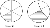
Figure 3.1: Bianchi I and II billiards are the shaded areas limited by curved lines or curvature walls and right lines or symmetry walls.

3. Bianchi–type VI₀: $\tilde{C}^{1}_{\,23}=1=\tilde{C}^{2}_{\,13}$.

The momentum constraints read

$$\pi^{{\scriptscriptstyle(3)}}{}_{{{\scriptscriptstyle(2)}}}=0\quad,\quad\pi^{{\scriptscriptstyle(3)}}{}_{{{\scriptscriptstyle(1)}}}=0\quad\mbox{and}\quad\pi^{{\scriptscriptstyle(2)}}{}_{{{\scriptscriptstyle(1)}}}+\pi^{{\scriptscriptstyle(1)}}{}_{{{\scriptscriptstyle(2)}}}=0.$$ (3.20)

They are equivalent to

$$0 = p_{2}$$ (3.21)

$$0 = p_{3}$$ (3.22)

$$0 = n_{1}(\pi_{{\scriptscriptstyle(2)}}-\pi_{{\scriptscriptstyle(1)}})+(e^{-2(\beta^{2}-\beta^{1})}-n_{1}^{2}+2)p_{1}.$$ (3.23)

The first two, according to (3.15) and (3.16), clearly tell that the symmetry walls $w_{32}=\beta^{3}-\beta^{2}$ and $w_{31}=\beta^{3}-\beta^{1}$ are absent from the potential. The billiard volume is therefore infinite (whether or not the last symmetry wall is present) and the asymptotic dynamics is described by a monotonic Kasner–like regime. With (3.22) put in (3.14), one sees that the coefficient of the third symmetry wall $w_{21}$ becomes $c_{12}=(p_{1})^{2}$. Since the constraint (3.23) does not imply that this coefficient vanishes, the corresponding wall will be generically present, i.e. for generic initial conditions.

Summarising, the symmetry wall $w_{21}=\beta^{2}-\beta^{1}$ is present, beside the two curvature walls $2\beta^{1}$ and $2\beta^{2}$; the dominant walls being $w_{21}=\beta^{2}-\beta^{1}$ and $2\beta^{1}$, they do not close the billiard, see Figure 3.2.

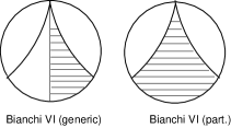
Figure 3.2: Bianchi VI Billiards

One can take advantage of the gauge freedom [25] to assign the initial value of $n^{0}_{1}$ to be zero, the constraint then implies that $p^{0}_{1}=0$. According to the equations of motion, $n_{1}$ and $p_{1}$ remain null. In particular, the last symmetry wall is absent and the billiard is delimited by two curvature walls depicted in Figure 3.2. The billiard shape will not depend on gauge choices for $d>3$.

These examples show that the presence/absence of symmetry walls may depend on initial conditions or on gauge conditions. This is not very satisfactory and suggest to analyse deeply the spatial diffeomorphisms in the generic case, i.e. non homogeneous. Nevertheless, in the cases mentionned hereabove, the finite/infinite nature of the billiard volume is not modified by a gauge choice.

4. Bianchi–type VII: $\tilde{C}^{1}_{\,23}=1,\quad\tilde{C}^{2}_{\,13}=-1$.

This case is very similar to the preceding one. The only changes are i) that the third constraint in (3.20) has to be replaced by ($\pi^{{\scriptscriptstyle(2)}}{}_{{{\scriptscriptstyle(1)}}}-\pi^{{\scriptscriptstyle(1)}}{}_{{{\scriptscriptstyle(2)}}}=0$) and ii) that its translation into the Iwasawa variables in (3.21) now reads

$$0=n_{1}(\pi_{{\scriptscriptstyle(2)}}-\pi_{1})+(e^{-2(\beta^{2}-\beta^{1})}-n_{1}^{2}-2)p_{1}\,.$$

Accordingly, we can apply the same reasoning as before.

5. Bianchi-type IX: $\tilde{C}^{1}_{\,23}=1,\quad\tilde{C}^{2}_{\,31}=1,\quad\tilde{C}^{3}_{\,12}=1$.

This case and the next one deserve a particular treatment because the structure constants are such that all curvature walls, namely $2\beta^{1}$, $2\beta^{2}$, $2\beta^{3}$, appear and these three gravitational walls already form a finite volume billiard.

Let us first discuss the generic case. The momentum constraints take the form

$$\pi^{{\scriptscriptstyle(3)}}{}_{{{\scriptscriptstyle(2)}}}-\pi^{{\scriptscriptstyle(2)}}{}_{{{\scriptscriptstyle(3)}}}=0,\quad\pi^{{\scriptscriptstyle(3)}}{}_{{{\scriptscriptstyle(1)}}}-\pi^{1}{}_{{{\scriptscriptstyle(3)}}}=0,\quad\pi^{{\scriptscriptstyle(2)}}{}_{{{\scriptscriptstyle(1)}}}-\pi^{{\scriptscriptstyle(1)}}{}_{{{\scriptscriptstyle(2)}}}=0\,;$$

and in terms of the Iwasawa variables, they become

$$n_{3}(\pi_{2} - \pi_{{\scriptscriptstyle(3)}})-n_{2}p_{1}+n_{1}p_{2}$$ (3.24)

$$+ [-e^{-2(\beta^{3}-\beta^{2})}+n_{3}^{2}+1]p_{3}=0$$

$$n_{2}(\pi_{{\scriptscriptstyle(3)}}-\pi_{{\scriptscriptstyle(1)}}) + n_{1}n_{3}(\pi_{{\scriptscriptstyle(2)}}-\pi_{{\scriptscriptstyle(3)}})+[n_{3}e^{-2(\beta^{2}-\beta^{1})}-n_{1}n_{2}]p_{1}$$ (3.25)

$$+ [e^{-2(\beta^{3}-\beta^{1})}+n_{3}^{2}e^{-2(\beta^{2}-\beta^{1})}-n_{2}^{2}-1]p_{2}$$

$$+ [n_{1}n_{3}^{2}-n_{2}n_{3}-n_{1}e^{-2(\beta^{3}-\beta^{2})}]p_{3}=0$$

$$n_{1}(\pi_{{\scriptscriptstyle(2)}} - \pi_{{\scriptscriptstyle(1)}})+[e^{-2(\beta^{2}-\beta^{1})}-n_{1}^{2}-2]p_{1}$$ (3.26)

$$+ [n_{3}e^{-2(\beta^{2}-\beta^{1})}-n_{1}n_{2}]p_{2}$$

$$+ [n_{1}n_{3}-n_{2}]p_{3}=0.$$

Remember that we already know that the billiard has a finite volume, hence the question is no longer to state between chaos or non chaos but rather to define more precisely the shape of the billiard.

In order to study the implications of the constraints (3.24) - (3.26), we shall rely on the heuristic estimates made in [44], where the asymptotic behaviour of the variables is analysed in the BKL limit. From that analysis, it follows that, when $\rho\to\infty$: i) the $\pi_{a}$’s go to zero as powers of $1/\rho$, ii) the $n_{i}$’s and the $p_{i}$’s tend to constants $n_{i}^{\infty}$ and $p_{i}^{\infty}$ up to additive terms which also go to zero as powers of $1/\rho$ and iii) that the exponentials either vanish (if the walls are present) or oscillate between zero and $\infty$ (if they are absent).

If the symmetry walls are absent, the constraints cannot be satisfied at any time. These walls are therefore generically present, i.e. they are present except if the coefficients in front of the exponential appearing in the constraints (3.24) - (3.26) are identically zero.

Accordingly, the billiard’s edge is formed by the leading symmetry walls $w_{32}$ and $w_{21}$ and by the curvature wall $2\beta^{1}$. On the Poincaré disc, it is one of the six small triangles included in the larger one bordered by the curvature walls. Its Cartan matrix is that of the hyperbolic Kac–Moody algebra $AE_{3}=A_{1}^{\wedge\wedge}$

$$\left(\begin{array}[]{ccc}2&-1&0\\ -1&2&-2\\ 0&-2&2\end{array}\right)$$

already relevant in the general inhomogeneous case. Its Dynkin diagram is given in Figure 3.3.

Figure 3.3: Dynkin diagrams of the $A_{1}^{\wedge\wedge}$ Kac–Moody algebra

Other interesting cases exist with less symmetry walls, which require specific initial conditions, see Figure 3.4.

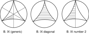
Figure 3.4: Bianchi IX Billiards

1. No symmetry wall at all. This situation is the one mentionned above; it happens when the metric is assumed diagonal always, hence for $n_{1}=0,n_{2}=0,n_{3}=0$; the solution of the momentum constraints is then $p_{1}=0,p_{2}=0,p_{3}=0$. This assumption is consistent with the equations of motion. The Cartan matrix of this billiard is given by

   $$\left(\begin{array}[]{ccc}2&-2&-2\\ -2&2&-2\\ -2&-2&2\end{array}\right)$$

   and its corresponding Dynkin diagram is number 1 in Figure 3.5 ; the associated Kac–Moody algebra is hyperbolic, it has number 7 in the enumeration provided in reference [155]. The billiard shape is depicted in Figure 3.4 (diagonal case).

2. One symmetry wall. This happens when one chooses the initial data such that $n_{1}=0,n_{2}=0$ and $p_{1}=0$, $p_{2}=0$; then, according to the equations of motion, these variables remains zero all the time. The billiard is closed by two curvature walls $2\beta^{1}$ and $2\beta^{2}$ and the symmetry wall $w_{32}$. On the Poincaré disc, its volume is half of that of the triangle made of curvature walls. The Cartan matrix is given by

   $$\left(\begin{array}[]{ccc}2&0&-2\\ 0&2&-2\\ -2&-2&2\end{array}\right)$$

   and its Dynkin diagram is number 2 in Figure 3.5 . It characterises the third rank 3 Lorentzian Kac–Moody algebra in the classification given in [155].

Figure 3.5: Dynkin diagrams of special algebras met in Bianchi IX models

These last two Kac–Moody algebras are subalgebras of $A_{1}^{\wedge\wedge}$ [75]. The billiard shape is depicted in Figure 3.4 (case number 2).

Remark: let us recall that the reflections on the faces of the billiard generate a Coxeter group which is identified with the Weyl group of the associated Kac–Moody algebra. The larger the set of walls, the larger the number of generators. Since in the non generic cases the set of walls is a subset of the one in the generic case, the associate Coxeter group is a subgroup of the generic one.

6. Bianchi–type VIII: $\tilde{C}^{1}_{\,23}=1,\quad\tilde{C}^{2}_{\,31}=1,\quad\tilde{C}^{3}_{\,12}=-1$.

The analysis of this case follows closely the previous one. The sign change in the structure constants modifies the constraints as follows

$$\pi^{{\scriptscriptstyle(3)}}{}_{{{\scriptscriptstyle(2)}}}+\pi^{{\scriptscriptstyle(2)}}{}_{{{\scriptscriptstyle(3)}}}=0,\quad\pi^{{\scriptscriptstyle(3)}}{}_{{{\scriptscriptstyle(1)}}}+\pi^{{\scriptscriptstyle(1)}}{}_{{{\scriptscriptstyle(3)}}}=0,\quad\pi^{{\scriptscriptstyle(2)}}{}_{{{\scriptscriptstyle(1)}}}-\pi^{{\scriptscriptstyle(1)}}{}_{{{\scriptscriptstyle(2)}}}=0$$

and induces some sign changes in their Iwasawa counterparts. The conclusions are those of the Bianchi IX model: the generic billiard is the one of the algebra $A_{1}^{\wedge\wedge}$.

3.2.3 $d=3$ Einstein–Maxwell Billiards

The momentum constraints (3.6) of the Einstein–Maxwell homogeneous models generally (except for the abelian Bianchi I) mix gravitational and one–form variables; in comparison with the pure gravity case, i) no constraint remains which clearly forces the prefactor of a symmetry wall to be zero and ii) additional terms of the type $\pi_{F\,{{\scriptscriptstyle(i)}}}F^{{{\scriptscriptstyle(i)}}{{\scriptscriptstyle(j)}}}$ enter in the constraints system.

Accordingly, generically, besides the curvature walls allowed by the structure constants, one expects all symmetry, electric and magnetic walls to be present. The dominant ones are the symmetry walls $w_{21}=\beta^{2}-\beta^{1},w_{32}=\beta^{3}-\beta^{2}$ and the electric wall $e_{1}=\beta^{1}$ which replaces the curvature wall of the pure gravity case. They close the billiard whose Cartan matrix is

$$\left(\begin{array}[]{ccc}2&-4&0\\ -1&2&-1\\ 0&-1&2\end{array}\right)\,.$$

The Dynkin diagram is dispayed in Figure 3.6; the corresponding Kac–Moody algebra is the hyperbolic $A_{2}^{(2)\wedge}$ algebra which is the Lorentzian extension of the twisted affine algebra $A_{2}^{(2)}$ also encountered in [89].

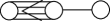
Figure 3.6: Dynkin diagram of the $A_{2}^{(2)\wedge}$ algebra

3.3 $d=4$ Homogeneous Models

Our billiard analysis of the four dimensional spatially homogeneous cosmological models has been carried out along the same lines as for $d=3$: results relative to pure gravity models and those relative to the Einstein–Maxwell homogeneous system will be given separately.

3.3.1 Extension of the Notations and Iwasawa Variables

In spatial dimension $d=4$, we introduce the matrix variables

$${\mathcal{N}}=\left(\begin{array}[]{cccc}1&n_{12}&n_{13}&n_{14}\\ 0&1&n_{23}&n_{24}\\ 0&0&1&n_{34}\\ 0&0&0&1\end{array}\right)\,.$$

The Iwasawa decomposition of the metric extends beyond the 3-dimensional formulae listed in (3.17), (3.18), (3.19), through the additional components

$$s_{{{\scriptscriptstyle(1)}}{{\scriptscriptstyle(4)}}} = n_{14}\,e^{-2\beta^{1}}$$

$$s_{{{\scriptscriptstyle(2)}}{{\scriptscriptstyle(4)}}} = n_{12}\,n_{14}\,e^{-2\beta^{1}}+n_{24}\,e^{-2\beta^{2}}$$

$$s_{{{\scriptscriptstyle(3)}}{{\scriptscriptstyle(4)}}} = n_{13}\,n_{14}\,e^{-2\beta^{1}}+n_{23}\,n_{24}\,e^{-2\beta^{2}}+n_{34}\,e^{-2\beta^{3}}$$

$$s_{{{\scriptscriptstyle(4)}}{{\scriptscriptstyle(4)}}} = n_{14}^{2}\,e^{-2\beta^{1}}+n_{24}^{2}\,e^{-2\beta^{2}}+n_{34}^{2}\,e^{-2\beta^{3}}+e^{-2\beta^{4}}\,.$$

The momentum conjugate to $\beta^{a}$ is written as $\pi_{{\scriptscriptstyle(a)}}$, as before; the momentum conjugate to ${\cal\tilde{N}}^{{\scriptscriptstyle(a)}}{}_{{{\scriptscriptstyle(j)}}}=n_{aj}$ is denoted ${\cal\tilde{P}}^{{\scriptscriptstyle(j)}}{}_{{{\scriptscriptstyle(a)}}}=p^{ja}$ and is only defined for $j>a$. The prefactors $c_{ab}=({\cal\tilde{P}}^{{\scriptscriptstyle(j)}}{}_{{{\scriptscriptstyle(a)}}}{\cal\tilde{N}}^{{\scriptscriptstyle(b)}}{}_{{{\scriptscriptstyle(j)}}})^{2}$ of the symmetry walls $e^{-2(\beta^{b}-\beta^{a})},b>a,$ in the Hamiltonian are explicitly given by

$$c_{12} = (p^{21}+p^{31}\,n_{23}+p^{41}\,n_{24})^{2}$$

$$c_{13} = (p^{31}+p^{41}\,n_{34})^{2}$$

$$c_{14} = (p^{41})^{2}$$

$$c_{23} = (p^{32}+p^{42}\,n_{34})^{2}$$

$$c_{24} = (p^{42})^{2}$$

$$c_{34} = (p^{43})^{2}\,.$$

Once the change of dynamical variables has been continued in a canonical point transformation, the momentum contraints still express linear relations among the $\pi^{{\scriptscriptstyle(i)}}{}_{{{\scriptscriptstyle(j)}}}$’s which translate into linear relations on the momenta $\pi_{{\scriptscriptstyle(a)}},p^{ia}$; their coefficients are polynomials in the $n_{ai}$’s times exponentials of the type $e^{-2(\beta_{b}-\beta_{a})}$, with $b>a$. The explicit form of the constraints depends on the model considered.

3.3.2 $d=4$ Pure Gravity

We label the various 4 dimensional spatially homogeneous models according to the classification of the 4 dimensional real unimodular Lie algebras given by M. MacCallum [128, 130]: they are

1. Class $U1[1,1,1]$: $\tilde{C}^{1}_{\,\,14}=\lambda,\,\tilde{C}^{2}_{\,\,24}=\mu,\,\tilde{C}^{3}_{\,\,34}=\nu,\mbox{with}\,\,\lambda+\mu+\nu=0$. One can still set $\lambda=1$ except in the abelian case where $\lambda=\mu=\nu=0$.

2. Class $U1[Z,\bar{Z},1]$: $\tilde{C}^{1}_{\,\,14}=-\frac{\mu}{2},\,\tilde{C}^{2}_{\,\,14}=1,\tilde{C}^{1}_{\,\,24}=-1,\,\tilde{C}^{2}_{\,\,24}=-\frac{\mu}{2},\ \tilde{C}^{3}_{\,\,34}=\mu.$ $\mu=0$ is a special case.

3. Class $U1[2,1]$: $\tilde{C}^{1}_{\,\,14}=-\frac{\mu}{2},\,\tilde{C}^{2}_{\,\,14}=1,\,\tilde{C}^{2}_{\,\,24}=-\frac{\mu}{2},\,\tilde{C}^{3}_{\,\,34}=\mu$ and $\mu$ is $0$ or $1$.

4. Class $U1[3]$: $\tilde{C}^{2}_{\,\,14}=1,\,\tilde{C}^{3}_{\,\,24}=1$.

5. Class $U3I0$: $\tilde{C}^{4}_{\,\,23}=1,\,\tilde{C}^{2}_{\,\,31}=1,\,\tilde{C}^{3}_{\,\,12}=-1.$

6. Class $U3I2$: $\tilde{C}^{4}_{\,\,23}=-1,\,\tilde{C}^{2}_{\,\,31}=1,\,\tilde{C}^{3}_{\,\,12}=1.$

7. Class $U3S1$ or $\mathfrak{sl}(2)\oplus\mathfrak{u}(1)$: $\tilde{C}^{1}_{\,\,23}=1,\,\tilde{C}^{2}_{\,\,31}=1,\,\tilde{C}^{3}_{\,\,12}=-1.$

8. Class $U3S3$ or $\mathfrak{su}(2)\oplus\mathfrak{u}(1)$: $\tilde{C}^{1}_{\,\,23}=1,\,\tilde{C}^{2}_{\,\,31}=1,\,\tilde{C}^{3}_{\,\,12}=1.$

Let us mention that for all of the four dimensional algebras, except of course the abelian one, the structure constant $\ C^{\prime 1}_{\,\,\,34}\neq 0$ and consequently that the curvature wall $2\beta^{1}+\beta^{2}$ is always present.

Our analysis leads to the conclusion that, from the billiard point of view, the previous models can be collected into two sets: the first one has an open billiard, the second one has a finite volume billiard whose Cartan matrix is that of the hyperbolic Kac–Moody algebra $A_{2}^{\wedge\wedge}$ exactly as in the general inhomogeneous situation.

The first set contains the abelian algebra and $U1[1,1,1]_{\mu\neq 0,-1}$, $U1[2,1]$ and $U1[Z,\bar{Z},1]_{\mu\neq 0}$; all the others belong to the second set. Because explicit developments soon become lenghty and since the reasonings always rest on similar arguments, we have chosen not to review systematically all cases as for $d=3$ but rather to illustrate the results on examples taken in both sets:

1. As a representative of the first set, we take $U1[Z,\bar{Z},1]_{\mu\neq 0}$.

The momentum constraints read

$$\pi^{{\scriptscriptstyle(4)}}{}_{{{\scriptscriptstyle(1)}}}=\pi^{{\scriptscriptstyle(4)}}{}_{{{\scriptscriptstyle(2)}}}=\mu\,\pi^{{\scriptscriptstyle(4)}}{}_{{{\scriptscriptstyle(3)}}}=-\frac{\mu}{2}(\pi^{{\scriptscriptstyle(1)}}{}_{{{\scriptscriptstyle(1)}}}+\pi^{{\scriptscriptstyle(2)}}{}_{{{\scriptscriptstyle(2)}}}-2\,\pi^{{\scriptscriptstyle(3)}}{}_{{{\scriptscriptstyle(3)}}}\,)+\pi^{{\scriptscriptstyle(1)}}{}_{{{\scriptscriptstyle(2)}}}-\pi^{{\scriptscriptstyle(2)}}{}_{{{\scriptscriptstyle(1)}}}=0\,;$$ (3.27)

in terms of the Iwasawa variables, they become

$$p^{41}=p^{42}=\mu\,p^{43}=0$$ (3.28)

and

$$- \frac{\mu}{2}(2\pi_{{\scriptscriptstyle(3)}}-\pi_{{\scriptscriptstyle(1)}}-\pi_{{\scriptscriptstyle(2)}})+n_{12}(\pi_{{\scriptscriptstyle(2)}}-\pi_{{\scriptscriptstyle(1)}})+$$ (3.29)

$$+ (e^{-2(\beta^{2}-\beta^{1})}-n_{12}^{2}-1)\,p^{21}+(n_{23}e^{-2(\beta^{2}-\beta^{1})}-n_{12}n_{13}+\frac{3n_{13}\mu}{2})p^{31}$$

$$+ (n_{12}n_{23}-n_{13}+\frac{3n_{23}\mu}{2})\,p^{32}=0\,.$$

The first three constraints (3.28) clearly indicate that the symmetry walls $\beta^{4}-\beta^{3}$, $\beta^{4}-\beta^{2}$, $\beta^{4}-\beta^{1}$ are absent from the potential. The fourth constraint (3.29) does not generically imply that $c_{23}=(p^{32})^{2}$ vanishes. Consequently, in the generic case, the dominant walls of the billiard are the symmetry walls $w_{32}=\beta^{3}-\beta^{2}$, $w_{21}=\beta^{2}-\beta^{1}$ and the curvature wall $2\beta^{1}+\beta^{2}$; it is indeed an open billiard.

Notice that in all cases of the first set, the non vanishing structure constants are all of the form $C^{\prime a}_{\hskip 4.26773pt4b}$ with $a,b=1,2,3$. It is easy to check that this forbids all curvature wall containing $\beta^{4}$ and therefore that the remaining curvature walls cannot be expected to close the billiard.

2. As a first representative of the second set, we take $U1[Z,\bar{Z},1]_{\mu=0}$

The constraints are given by (3.27), (3.28) and (3.29) for $\mu=0$ and one immediately sees that, compared to the preceding case, one constraint drops out leaving the symmetry wall $w_{43}=\beta^{4}-\beta^{3}$ in place. The last constraint does not generically imply the vanishing of other prefactors $c_{ab}$. Again, we end up here with the following list of dominant walls: $w_{43}=\beta^{4}-\beta^{3}$, $w_{32}=\beta^{3}-\beta^{2}$, $w_{21}=\beta^{2}-\beta^{1}$ and $2\beta^{1}+\beta^{2}$. The Cartan matrix is that of the algebra $A_{2}^{\wedge\wedge}$ as previously announced. Its Dynkin diagram is depicted in Figure 3.7.

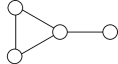
Figure 3.7: Dynkin diagram of the $A^{\wedge\wedge}_{2}$ algebra

3. Another interesting example of the second set is provided by $U3S3$

Its homogeneity group is the direct product $SU(2)\times U(1)$ so that this model appears as the four dimensional trivial extension of the Bianchi IX model: since the structure constants are the same as in the 3-dimensional case, the momentum constraints do not change, when expressed in terms of the metric components and their momenta

$$\pi^{{\scriptscriptstyle(1)}}{}_{{\scriptscriptstyle(3)}}-\pi^{{\scriptscriptstyle(3)}}{}_{{\scriptscriptstyle(1)}}=0,\quad\pi^{{\scriptscriptstyle(1)}}{}_{{\scriptscriptstyle(2)}}-\pi^{{\scriptscriptstyle(2)}}{}_{{\scriptscriptstyle(1)}}=0,\quad\pi^{{\scriptscriptstyle(2)}}{}_{{\scriptscriptstyle(3)}}-\pi^{{\scriptscriptstyle(3)}}{}_{{\scriptscriptstyle(1)}}=0\,;$$

their number does not change either but, in terms of Iwasawa variables, they involve much more terms than their $d=3$ counterpart given in (3.24), (3.25) and (3.26)

$$- n_{13}(\pi_{{\scriptscriptstyle(1)}}-\pi_{{\scriptscriptstyle(3)}})+n_{12}n_{23}(\pi_{{\scriptscriptstyle(2)}}-\pi_{{\scriptscriptstyle(3)}})-(n_{12}n_{13}-n_{23}e^{-2(\beta^{2}-\beta^{1})})p^{21}$$

$$- (n_{13}^{2}-n_{23}^{2}e^{-2(\beta^{2}-\beta^{1})}-e^{-2(\beta^{3}-\beta^{1})}-1)p^{31}$$

$$+ (n_{12}n_{23}^{2}-n_{13}n_{23}-n_{12}e^{-2(\beta^{3}-\beta^{2})})p^{32}$$

$$- (n_{13}n_{14}-n_{23}e^{-2(\beta^{2}-\beta^{1})}n_{24}-n_{34}e^{-2(\beta^{3}-\beta^{1})})p^{41}$$

$$+ (n_{12}n_{23}n_{24}-n_{14}n_{23}-n_{12}n_{34}e^{-2(\beta^{3}-\beta^{2})})p^{42}$$

$$- (n_{12}n_{23}n_{34}-n_{12}n_{24}-n_{13}n_{34}+n_{14})p^{43}=0$$

$$- n_{12}(\pi_{{\scriptscriptstyle(1)}}-\pi_{{\scriptscriptstyle(2)}})-(n_{12}^{2}-e^{-2(\beta^{2}-\beta^{1})}-1)p^{21}$$

$$- (n_{12}n_{13}-n_{23}e^{-2(\beta^{2}-\beta^{1})})p^{31}+(n_{12}n_{23}-n_{13})p^{32}$$

$$- (n_{12}n_{14}-n_{24}e^{-2(\beta^{2}-\beta^{1})})p^{41}+(n_{12}n_{24}-n_{14})p^{42}=0$$

$$- n_{23}(\pi_{{\scriptscriptstyle(2)}}-\pi_{{\scriptscriptstyle(3)}})+n_{13}p^{21}-n_{12}p^{31}-(n_{23}^{2}-e^{-2(\beta^{3}-\beta^{2})}+1)p^{32}$$

$$- (n_{23}n_{24}-n_{34}e^{-2(\beta^{3}-\beta^{2})})p^{42}+(n_{23}n_{34}-n_{24})p^{43}=0\,.$$

These constraints are of course i) linear in the momenta, ii) the only exponentials which enter these expressions are build of $w_{32}=\beta^{3}-\beta^{2}$, $w_{31}=\beta^{3}-\beta^{1}$ and $w_{21}=\beta^{2}-\beta^{1}$ and iii) as before, their coefficients are exactly given by the square root of the corresponding $c_{A}$’s in the potential, namely $\sqrt{c_{12}},\sqrt{c_{13}}$ and $\sqrt{c_{23}}$. Accordingly, the question arises whether these equations are equivalent to $c_{12}=0$, $c_{23}=0$ and $c_{13}=0$. If, asymptotically, the exponentials go to zero and can be dropped out of the constraints, the remaining equations can be solved for $p^{21},p^{31},p^{32}$ in terms of the other variables among which figure now, not only the $\pi_{{\scriptscriptstyle(i)}}-\pi_{{\scriptscriptstyle(j)}}$ already present in the 3-dimensional case which asymptotically go to zero, but also the asymptotic values of the $p^{4i}$’s which remain unconstrained. It follows that none of the solutions of the above system is generically forced to vanish so that all the symmetry walls are expected to be present. The absence of a wall can only happen in non generic situations with very peculiar initial conditions.

We expect this result to become the rule in higher dimensions for trivial extensions like $SU(2)\times SU(2)\times...\times U(1)\times...\times U(1)$; the billiard will then become that of the Kac–Moody algebra $A_{n}^{\wedge\wedge}$ relevant in the general Einstein theory.

We can nevertheless provide a particular solution with initial data obeying $n_{12}=n_{13}=n_{14}=0$ and $p^{21}=p^{31}=p^{41}=0$. These values are conserved in the time evolution. In this case, the leading walls are the symmetry walls $w_{43},w_{32}$ and the curvature ones $2\beta^{2}+\beta^{3},2\beta^{1}+\beta^{2}$. The Cartan matrix is

$$\left(\begin{array}[]{cccc}2&-1&-1&0\\ -1&2&-1&-1\\ -1&-1&2&-1\\ 0&-1&-1&2\\ \end{array}\right)\,.$$

The billiard is characterised by the rank 4 Lorentzian Kac–Moody algebra which bears number 2 in the classification given in [155] and which is a subalgebra of $A_{2}^{++}$; its Dynkin diagram is drawn in Figure 3.8.

Figure 3.8: Dynkin diagram of algebra number 2 in the subset of rank 4

The $D=5$ results are summarized in the following table:

$U1[1,1,1]_{\mu=\nu=\lambda=0}$ $U1[1,1,1]_{\mu\neq 0,-1}$ $U1[Z,\bar{Z},1]_{\mu\neq 0}$	non chaotic
$U1[1,1,1]_{\mu=-1}$ $U1[Z,\bar{Z},1]_{\mu=0}$ $U1[2,1]$ $U1[3]$ $U3I0$ $U3I2$ $U3S3$ $U3S1$	chaotic

Chaos or non chaos for $D=5$ models

3.3.3 $d=4$ Einstein–Maxwell Models

As in the three dimensional case, because of the presence of the electromagnetic field in the expression of the momentum constraint (3.6), no symmetry wall can be eliminated. Moreover, the electric walls always prevail over the curvature ones if any. The billiard is in all cases characterised by the following set of dominant walls $w_{43}=\beta^{4}-\beta^{3}$, $w_{32}=\beta^{3}-\beta^{2}$, $w_{21}=\beta^{2}-\beta^{1}$ and $e_{1}=\beta^{1}$. Its Cartan matrix is that of the hyperbolic Kac–Moody algebra $G^{\wedge\wedge}_{2}$ with Dynkin diagram depicted in Figure 3.9.

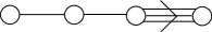
Figure 3.9: Dynkin diagram of the $G^{\wedge\wedge}_{2}$ algebra

In the general analysis of the billiards attached to coupled gravity + p–forms systems, one could assume $2p<d$ without loss of generality, because the complete set of walls is invariant under electric–magnetic duality. This invariance may however not remain in some spatially homogeneous cases due to the vanishing of some structure constants which lead to incomplete sets of walls so that other, a priori unexpected Kac–Moody algebras, might appear. An illustrative and interesting example is given in $D=5$ by the Einstein + $2$–form system governed by the abelian algebra. Here, the dominant walls are i) the symmetry walls $\beta^{4}-\beta^{3}$, $\beta^{3}-\beta^{2}$ and $\beta^{2}-\beta^{1}$ and ii) the magnetic wall $\beta^{1}+\beta^{2}$. This billiard brings in the new hyperbolic Kac–Moody algebra carrying number 20 in [155], whose Dynkin diagram is given in Figure 3.10 hereafter.

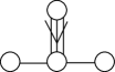
Figure 3.10: Dynkin diagram of the algebra relevant for the Einstein + $2$–form system

3.4 Conclusions

In this chapter, we have analysed the Einstein and Einstein–Maxwell billiards for all the spatially homogeneous cosmological models in 3 and 4 dimensions. In the billiard picture, we confirm that in spacetime dimensions $5\leq D\leq 10$, diagonal models are not rich enough to produce the never ending oscillatory behaviour of the generic solution of Einstein’s equations and that chaos is restored when off-diagonal metric elements are kept. Chaotic models are characterised by a finite volume billiard which can be identified with the fundamental Weyl chamber of an hyperbolic Kac–Moody algebra: in the most generic chaotic situation, the algebra coincides with the one already relevant in the inhomogeneous case; this remains true after the addition of an generic homogeneous electromagnetic field. Other algebras can also appear for special initial data or gauge choices: in fact, these are all the simply-laced known hyperbolic Kac–Moody algebras of ranks 3 and 4, except the one which has number 3 among those of rank 4 listed in [155]. This analysis furnishes a nice way to tackle infinite–dimensional hyperbolic subalgebras of those appearing in the non–homogeneous context.

Chapter 4 Oxidation

An interesting feature of the billiard region is that it is invariant under toroidal dimensional reduction to any dimension $D\geq 3$ [37]. The knowledge the billiard region in $D=3$ dimensions can then be used as a tool to determine the possible higher dimensional parents of the theory. This problem of going up in dimension is known as the oxidation or disintegration problem and goes back to the early days of supergravity and has been studied repeatedly [107, 103, 108]. It has been thoroughly investigated recently by means of group theory techniques [110, 111, 112]. We show here that the billiard approach gives direct information on possible obstructions to oxidation and, when oxidation is possible, restricts efficiently the maximal dimension(s) of oxidation as well as determines the full $p$–form spectrum of the maximally oxidised theory. We consider both split and non–split ${\cal U}_{3}$–groups. For non maximally non–compact groups (i.e. non–split groups), this approach is complementary to the general method of general linear subgroups of [108] known as the “A–chain” method. The same information can be extracted from the superalgebra approach to the problem [50, 93, 92, 91].

4.1 Walls associated with simple roots and oxidation

The walls bounding the billiards have different origins: they can be symmetry (2.28) or curvature walls (2.29 & 2.30), related to the Einstein–Hilbert action; or they can be $p$–form walls (electric (2.31) or magnetic (2.32)), related to the $p$–form part of the action. The key to the derivation of the oxidation constraints is to investigate how the billiard walls behave upon dimensional reduction. Although the billiard region is invariant, the formal origin of the walls may change. E.g., a symmetry wall in $D$ dimensions may appear as a $1$–form wall associated with the Kaluza–Klein graviphoton(s) in lower dimensions [41].

The translation rules relating walls in higher dimensions to walls in lower dimensions have been worked out in [37, 89]. To recall them, we denote by $\bar{B}$ the restricted root system of the real form ${\cal U}_{3}$. This restricted root system may be reduced or non reduced, in the latter case it is of $BC_{r}$–type [85]. The billiard region is the fundamental Weyl chamber of the overextension $\bar{B}^{\wedge\wedge}$ [89] obtained by adding to the simple roots of the finite root system $\bar{B}$, the affine root $\alpha_{0}$ and the “overextended root” $\alpha_{-1}$, which is attached to the affine root with a single link. There are at most two different root lengths, except when the underlying finite root system is non reduced, in which case one has three different root lengths. The highest root is always a long root (“very long” root in the $BC_{r}$–case) [89].

From the point of view of the three–dimensional action (Einstein–Hilbert action + ${\cal U}_{3}$–non linear $\sigma$-model action), these roots have the following interpretation: (i) the overextended root is the symmetry wall $\beta^{2}-\beta^{1}$ and involves only gravitational variables; (ii) the affine root corresponds to the dominant magnetic wall $\beta^{1}-\theta(\phi)$ where $\theta(\phi)$ is the highest root of ${\bar{B}}$; it involves both the dilatons and the gravitational variable $\beta^{1}$; and (iii) the simple roots of $\bar{B}$ correspond to the dominant electric walls defined by the $0$–forms (axions) and involve the dilatons only.

In $D=d+1>3$ dimensions, these walls appear as follows. (i) The overextended root remains a symmetry wall, namely $\beta^{d}-\beta^{d-1}$; (ii) The affine root becomes the symmetry wall $\beta^{d-1}-\beta^{d-2}$. (iii) The (long) roots of ${\bar{B}}$ connected to the affine root by a chain of single links form a chain of symmetry walls $\beta^{d-2}-\beta^{d-3}$, $\cdots$, $\beta^{2}-\beta^{1}$. The other roots correspond to $p$–form walls of the form $\beta^{1}+\cdots+\beta^{p}+\frac{1}{2}\sum_{\alpha}\lambda^{(p)}_{\alpha}\phi^{\alpha}$ (electric walls) or $\beta^{1}+\cdots+\beta^{d-p-1}-\frac{1}{2}\sum_{\alpha}\lambda^{(p)}_{\alpha}\phi^{\alpha}$ (magnetic walls). In these equations, the $\lambda^{(p)}_{\alpha}$ are the couplings to the dilatons $\phi^{\alpha}$ present in $D$ dimensions (if any).

4.2 Obstructions to oxidation

A crucial feature of the gravitational walls (symmetry and curvature walls) is that they are non degenerate. By contrast, the $p$–form walls may come with a non trivial multiplicity since one can include many $p$–forms with the same degree and same dilaton couplings.

It follows from this observation that a “necessary condition” for oxidability of a $3$–dimensional theory to $D>3$ dimensions is that the (very) long roots of $\bar{B}$ must be non degenerate, since the affine root, which is the magnetic wall $\beta^{1}-\theta(\phi^{\Delta})$ in three dimensions, becomes a symmetry wall in $D>3$ dimensions (and the degeneracy of $\beta^{1}-\theta(\phi^{\Delta})$ is the degeneracy of the (very) long highest root $\theta(\phi^{\Delta})$). This necessary condition on the highest root was spelled out in [89]. It provides an obstruction to oxidation to $D>3$ dimensions for the following cases (see [85]) for conventions):

$A\;II$ ($SU^{*}(2n)/Sp(n)$) for which $m_{\theta}=4$; $B\;II$ and $D\;II$ ($SO(p,1)$) for which $m_{\theta}=p-1$; $C\;II$ ($Sp(p,q)/Sp(p)\times Sp(q))$ for which $m_{\theta}=3$; $E\;IV$ ($E_{6(-28)}/F_{4}$) for which $m_{\theta}=8$; and $F\;II$ ($F_{4(-20)}/SO(9)$) for which $m_{\theta}=7$. Here, $m_{\theta}$ is the multiplicity of the highest root $\theta$. That these non–split theories cannot be oxidised agrees with the findings of [19, 111].

Note that this list is precisely the list of real forms whose Satake diagrams have a “compact” Cartan generator at the simple root(s) that connects (or connect) to the affinizing root or equivalently that is not orthogonal to the most negative root of the simple Lie algebra under consideration. Affinization occurs in 2 dimensions; in the build-up of the $SL(D_{max}-3,R)\times R$ chain one would expect the dilation of the fourth coordinate to be a noncompact Cartan generator at that vertex as soon as $D_{max}\geq 4$ [108]. Conversely the fact that the root before the affinizing one is noncompact, to use approximate language, seems to imply that the affine root is noncompact too and can participate in a $GL(D_{max}-2,R)$ group of duality symmetries [108].

Finally, we note that the $C\;II$ (with $q=2$) and $F\;II$ cases have a supersymmetric extension with an odd number of $3$–dimensional supersymmetries ($N=5$ and $N=9$, respectively) [60]. These supersymmetries cannot come from four dimensions since a four–dimensional theory yields an even number of supersymmetries in $D=3$. Our obstruction to oxidation given above does not rely on supersymmetry, however, and prevents even non-supersymmetric “parents”.

4.3 Maximal dimensions

When the theory can be oxidised, one can infer the maximal dimension(s) in which it can be formulated from the rules recalled above: this is $D_{max}=k+2$ where $k$ is the length of the symmetry wall chain, i.e. the length of the single-linked chain of nodes in the Dynkin diagram of the restricted root system $\bar{B}^{\wedge\wedge}$ that can be constructed starting from the overextended root, without loop (hereafter called “A–chain”). If there is a fork, each branch yields an independent maximal dimension. By mere inspection of the tables and Satake diagrams in [85] and of the Dynkin diagrams of the overextensions given e.g. in [37, 89], one easily gets the results collected in the Table 4.1.

Table 4.1:

Class	Noncompact Symmetric Space D=3	$D_{max}$
$A\;I$	$SL(r+1)/SO(r+1)$	$r+3$
$A\;III$ and $A\;IV$	$SU(p,q)/(S(U_{p}\times U_{q}))$	$4$
$B\;I$ and $D\;I$	$SO(p,q)/(SO(p)\times SO(q))$, $p\geq q>1$	$q+2$ and $6$ ($q\geq 3$)
$C\;I$	$Sp(n,R)/U(n)$	$4$
$D\;III$	$SO^{*}(2n)/U(n)$	$4$
$E\;I$	$E_{6(6)}/Sp(4)$	$8$
$E\;II$	$E_{6(2)}/(SU(6)\times SU(2))$	$6$
$E\;III$	$E_{6(-14)}/(SO(10)\times U(1))$	4
$E\;V$	$E_{7(7)}/SU(8)$	$8$ and $10$
$E\;VI$	$E_{7(-5)}/(SO(12)\times SU(2))$	6
$E\;VII$	$E_{7(-25)}/(E_{6(-78)}\times U(1))$	4
$E\;VIII$	$E_{8(8)}/SO(16)$	10 and 11
$E\;IX$	$E_{8(-24)}/(E_{7(-133)}\times SU(2))$	6
$F\;I$	$F_{4(4)}/(Sp(3)\times SU(2))$	6
$G$	$G_{2(2)}/SO(4)$	5

The “necessary condition” that we used is à priori not sufficient but it is supported by the inspection of the literature. Indeed, in all maximal oxidation dimensions, a theory which correctly reduces to $D=3$ actually exists. These theories are listed in [111] in terms of previously constructed models ([19, 30, 156, 61, 49, 62]).

4.4 $p$–form spectrum and oxidation

The billiard provides also information on the $p$–forms that must be present in the maximal oxidation dimension because one knows how the $p$–form walls must connect to the A–chain. A simple electric $p$–form wall connects to the $p$–th root in the A–chain (counting now from the root at the end of the A–chain opposite to the overextended root). A simple magnetic $p$–form wall connects to the $(d-p-1)$–th root. One also knows the multiplicities. Together with the Weyl group, this can be used to construct the $p$–form spectrum and determine the dilaton couplings.

Rather than deriving explicitly all cases, we shall focus on $E\,\;IX$, i.e., $E_{8(-24)}/(E_{7(-133)}\times SU(2))$, which has a restricted root system of $F_{4}$–type

The other cases are treated similarly and reproduce known results. The root $\alpha_{-1}$ in the above Dynkin diagram is the overextended root, the root $\alpha_{0}$ is the affine root, while $\alpha_{1}$ and $\alpha_{2}$ are the long roots of $F_{4}$. The roots $\alpha_{-1},\alpha_{0},\alpha_{1},\alpha_{2}$ have multiplicity $1$. The roots $\alpha_{3}$ and $\alpha_{4}$ are the short roots and have multiplicity $8$ [85]. The A–chain is given by the roots $\alpha_{-1},\alpha_{0},\alpha_{1},\alpha_{2}$, which read, in $D_{max}=6$ dimensions, $\alpha_{2}=\beta^{2}-\beta^{1}$, $\alpha_{1}=\beta^{3}-\beta^{2}$, $\alpha_{0}=\beta^{4}-\beta^{3}$ and $\alpha_{-1}=\beta^{5}-\beta^{4}$. Since $F^{\wedge\wedge}_{4}$ has rank $6$ and since there is only five logarithmic scale factors, one needs one dilaton.

Because the short root $\alpha_{3}$ is attached to the first root $\alpha_{2}$ of the A–chain, it corresponds to the electric wall of a $1$–form. Requiring that the root has length squared equal to one (one has $(\alpha_{2}|\alpha_{2})=2$ and $(\alpha_{2}|\alpha_{3})=-1$) fixes the dilaton coupling of the one–form to $\lambda^{(1+)}=-1$, i.e., $\alpha_{3}=\beta^{1}-(\phi/2)$. The last simple root $\alpha_{4}$ is not attached to the A–chain: it corresponds therefore to an axion, with dilaton coupling equal to $\lambda^{(0)}=2$, i.e., electric $0$–form wall $\alpha_{4}=\phi$. The degeneracy of the short roots is $8$; hence, at this stage, we need eight $1$–forms and eight $0$–forms.

This is not the entire spectrum of $p$–forms because we have only accounted so far for the simple roots. There are other positive roots in the theory which correspond also to walls of the $p$–form type, as can be seen by acting with the finite Weyl group of $F_{4}$ (= restricted Weyl group of ${\cal U}_{3}$) on the roots $\alpha_{1}$, $\alpha_{2}$, $\alpha_{3}$ and $\alpha_{4}$. These roots must be included by incorporating the corresponding $p$–forms.

By Weyl–reflecting the short root $\alpha_{3}=\beta^{1}-(\phi/2)$ in $\alpha_{4}$, we get the root $\beta^{1}+(\phi/2)$. This is also an electric $1$–form wall, with degeneracy $8$. We thus need eight further $1$–forms, with dilaton couplings $\lambda^{(1-)}=1$. We then observe that the symmetry wall reflection in $\beta^{2}-\beta^{1}$ replaces $\beta^{1}-(\phi/2)$ by $\beta^{2}-(\phi/2)$. Reflecting this root in $\beta^{1}+(\phi/2)$ yields $\beta^{1}+\beta^{2}$, which is the electric (= magnetic) wall of a chiral $2$–form with zero dilaton coupling. This root is short, so again degenerate $8$ times: we need eight such chiral $2$–forms (or four non–chiral $2$–forms with zero dilaton couplings). Finally, by reflecting in $\alpha_{3}$ the long root $\beta^{2}-\beta^{1}$, we generate the long root $\beta^{1}+\beta^{2}-\phi$. This is an electric wall for a $2$–form with dilaton coupling $\lambda^{(2)}=-2$, which we must include. A reflection in $\alpha_{4}$ yields $\beta^{1}+\beta^{2}+\phi$ but this is just a magnetic root for the same $2$–form, so we do not need any further additional field to get these walls in the Lagrangian. Similarly, the short roots $\beta^{1}+\beta^{2}+\beta^{3}\pm(\phi/2)$ obtained by reflecting $\beta^{3}\pm(\phi/2)$ in $\beta^{1}+\beta^{2}$ are the magnetic walls of the $1$–forms and do not need new fields either. [Note in passing the obvious misprints in formulas (6.21) and (6.22) for the magnetic walls of the $2$–forms in [37]. (Also the magnetic walls of $G_{2}$ are miswritten there).]

To summarise: by acting with the finite Weyl group of $F_{4}$ on the simple roots $\alpha_{1}$, $\alpha_{2}$, $\alpha_{3}$ and $\alpha_{4}$, we get all the roots of $F_{4}$. The positive roots, which must have a term in the Lagrangian, are $\beta^{i}-\beta^{j}$ ($i>j)$ (long), $\phi$ (short), $\beta^{i}\pm(\phi/2)$ (short), $\beta^{i}+\beta^{j}$ ($i<j$) (short), $\beta^{i}+\beta^{j}\pm\phi$ ($i<j$) (long), $\beta^{i}+\beta^{j}+\beta^{k}\pm(\phi/2)$ ($i<j<k$) (short) and $2\beta^{i}+\beta^{j}+\beta^{k}$ ($i\not=j$, $i\not=k$, $j<k$) (long). Here, $i,j,k\in\{1,2,3\}$. These are all the $24$ positive roots of $F_{4}$. They are all accounted for by the $p$–form walls, except the last ones, which are curvature walls following from the Einstein–Hilbert action (and the symmetry walls). By acting with the $F_{4}^{\wedge\wedge}$–Weyl reflections associated with the other symmetry walls, one covariantizes the above expressions (i.e., one generates the same walls but with $i,j,k\in\{1,2,3,4,5\}$). Continuing, i.e. acting with the other elements of the infinite Weyl group of $F_{4}^{\wedge\wedge}$, one generates new walls but these are not of the $p$–form type because they necessarily contain a $\beta^{i}$ with a coefficient at least 2 (except the magnetic walls $\beta^{i}+\beta^{j}+\beta^{k}+\beta^{m}-\phi$ ($i<j<k<m$) of the $0$–form and the null magnetic walls $\beta^{i}+\beta^{j}+\beta^{k}+\beta^{m}$ of the dilaton, but these are already accounted for). All the $p$–form roots have been exhausted.

We mention that the superalgebra approach gives an alternative procedure to generate the $p$–spectrum from the Borcherds–Chevalley–Serre relations and also provides detailed information on the Chern–Simons terms in the Lagrangian (as the group theory approach [110, 111, 112] and the principles given in [74] do). See [93, 91] for the split case and [92, 91] for the non split case.

4.5 Results and comments

We have shown in this chapter how the billiard analysis of gravitational theories, related to Satake diagrams and restricted root systems [89], provides useful information on their oxidation endpoint both in the split and in the non–split cases.

It is noteworthy that the split real forms allow oxidation by at least one dimension, to $D\geq 4$. One is stuck to $D=3$ only for certain non–split real forms, because of the non trivial multiplicities of the (very) long roots (which are always non-degenerate in the split case). The constraint on multiplicities provides a rather powerful insight. Finally, we mention the paper [77] which also deals with ${\cal U}_{3}$, billiards and oxidation.

Chapter 5 Hyperbolic Algebras

A criterion for the gravitational dynamics to be chaotic is that the billiard has a finite volume. This in turn stems from the remarkable property that the billiard can be identified with the fundamental Weyl chamber of an hyperbolic Kac–Moody algebra. The purpose of this chapter is twofold: first we determine all hyperbolic Kac–Moody algebras for which a billiard description exists and then we explicitly construct all Lagrangians describing gravity coupled to dilatons and $p$–forms producing these billiards.

We are able to give exhaustive results because (i) the hyperbolic algebras are all known and classified [155], and (ii) only the finite number of algebras with rank $r$ between $3$ and $10$ are relevant in this context. Note that there are infinitely many hyperbolic algebras of rank two and that there exists no hyperbolic algebra of rank $r>10$. The analysis is considerably simplified because of the invariance of the billiard under toroidal dimensional reduction to dimensions $D\geq 3$, see [37]. Indeed, the billiard region remains the same, but a symmetry wall in $D$ dimensions may become an electric or magnetic $p$–form wall in a lower dimension (see previous chapter). The invariance under dimensional reduction implies in particular that the determination of algebras with a billiard description can be performed by analysing Lagrangians in $D=3$ dimensions.

Simplifications in $D=3$ occur because only $0$–forms are present: indeed, via appropriate dualisations, all $p$–forms can be reduced to $0$–forms. To be concrete, for the hyperbolic algebras of real rank $r$ between $3$ and $6$, we first try to reproduce their Dynkin diagram with a set of $r$ dominant walls comprising one symmetry wall (2.28) ($\beta^{2}-\beta^{1})$ and $(r-1)$ scalar walls (Eqs. (2.31) $\&$ (2.32) for $p=0$). If this can be done, we still have to check that the remaining walls are subdominant, i.e. that they can be written as linear combinations of the dominant ones with positive coefficients. In particular, this analysis requires that any dominant set necessarily involves one magnetic wall and $(r-2)$ electric walls, as will become clear by focussing on an example. To deal with the hyperbolic algebras of ranks $7$ to $10$, it is actually not necessary to first reduce to 3 dimensions: the overextensions of finite simple Lie algebras have already been associated to billiards of some Lagrangians and for the remaining four algebras, the rules we have found in the previous cases allow to straightforwardly construct the Lagrangian in the maximal oxidation dimension.

We then analyse which three–dimensional system admits parents in higher dimensions and construct the Lagrangian in the maximal oxidation dimension. In order to do so, we take an algebra in the previous list and we determine successively the maximal spacetime dimension, the dilaton number, the $p$–form content and the dilaton couplings:

1. One considers the Dynkin diagram of the selected algebra and looks at the length of its ”A–chain”, starting with the only symmetry root in $D=3$. Our analysis produces the following oxidation rule: if the A–chain has length $k$, the theory can be oxidised up to

   1. $D_{max}=k+2$, if the root(s) attached to the end of the A–chain have a norm squared smaller than $2$,

   2. $D_{max}=k+1$, if the root(s) attached to the end of the A–chain have a norm squared greater than $2$.

   This generalises the oxidation rule by [50] and [110, 111, 112], obtained by group theoretical arguments applied to coset models.

2. For given space dimension $d=D-1$ and rank $r$ of the algebra, the number of dilatons is given by $n=r-d$ because the dominant walls are required to be $r$ independent linear forms in the $d$ scale factors $\{\beta^{1},...,\beta^{d}\}$ and the $n$ dilatons.

3. Because it is known how the $p$–form walls connect to the A–chain [37], one can read on the Dynkin diagram which $p$–forms appear in the maximal oxidation dimension.

4. The dilaton couplings of the $p$–forms are computed from the norms and scalar products of the walls which have to generate the Cartan matrix of the hyperbolic algebra. This means in particular that, even if the nature of the walls changes during the oxidation procedure, their norms and scalar products remain unchanged. Note also that in all dimensions $D>3$ the subdominant conditions are always satisfied.

As a byproduct of our analysis, we note that, for each billiard identifiable as the fundamental Weyl chamber of an hyperbolic algebra, the positive linear combinations of the dominant walls representing the subdominant ones only contain integer coefficients. Hence, the dominant walls of the Lagrangian correspond to the simple roots of the hyperbolic algebra, while the subdominant ones correspond to non simple positive roots.
Note however that even the 3–dimensional scalar Lagrangians do not describe coset spaces in general. Nevertheless, the reflections relative to the simple roots generate the Weyl group of the hyperbolic algebra; this group in turn gives an access to other positive roots and suggests that a Lagrangian capable to produce these roots via billiard walls needs more exotic fields than just $p$–forms.

This chapter is organized as follows. In the four sections, we deal with hyperbolic algebras of rank 3 to 6. First, in $D=3$ spacetime dimensions, we compute the 3–dimensional dilaton couplings needed to reproduce the Dynkin diagram and check the status of the subdominant walls. This is how we select the admissible algebras. Next, for each of them, we determine which Lagrangian can be oxidised and we produce it in the maximal oxidation dimension. The 18 hyperbolic algebras of ranks 7 to 10 are reviewed in the last section; as explained before, they are singled out for special treatment because 14 of them are overextensions of finite dimensional simple Lie algebras and the remaining 4 are dual to the overtextension $B_{n}^{\wedge\wedge}$ (with $n=5,6,7,8$). We explicitly write down the $D_{max}=9$ Lagrangian system obtained previously in [88] the billiard of which is the fundamental Weyl chamber of the algebra $CE_{10}$. Among the four hyperbolic algebras of rank 10, $CE_{10}$ is special because, unlike $E_{10},BE_{10}$ and $DE_{10}$, it does not stem from supergravities.

5.1 Rank 3, 4, 5 and 6 Hyperbolic Algebras

Rank 3 Hyperbolic algebras: $D=3$

In space dimension $d=2$, one has a single symmetry wall (2.28), namely

$$\alpha_{1}=\beta^{2}-\beta^{1}$$

and $n=r-d=3-2=1$ dilaton denoted as $\phi$. Since we do not consider pure gravity (as it is already known), the dominant walls are $p$–form walls, i.e. in the present $d=2$ case $0$–form walls. It is obvious that only a $0$–form magnetic wall (2.32) can be connected to the symmetry wall (see the form of the metric (2.22) and of the 0–form electric walls (2.31)), say

$$\alpha_{2}=\beta^{1}-\tilde{\lambda}\phi\ .$$

Let us show that the last dominant wall has to be an electric one denoted by

$$\alpha_{3}=\tilde{\lambda}^{\prime}\phi\ .$$ (5.1)

Indeed, had we taken for dominant the magnetic wall $\tilde{\alpha}_{3}=\beta^{1}-\tilde{\lambda}^{\prime}\phi$ instead of (5.1), then its corresponding electric wall (which is precisely $\alpha_{3}=\tilde{\lambda}^{\prime}\phi$) would be dominant too because of the impossibility to write it as a linear combination with positive coefficients of the three others $\alpha_{1},\alpha_{2}$ and $\tilde{\alpha}_{3}$. Since we are interested in $r=3$ algebras, we only want three dominant walls.

Using the metric (2.22) adapted to $d=2$, we build the matrix (2.33)

$$A_{ij}=2{(\alpha_{i}|\alpha_{j})\over(\alpha_{i}|\alpha_{i})}$$

and obtain

$$A=\left(\begin{array}[]{ccc}2&-1&0\\ -{2\over\tilde{\lambda}^{2}}&2&-2{\tilde{\lambda}^{\prime}\over\tilde{\lambda}}\\ 0&-2{\tilde{\lambda}\over\tilde{\lambda}^{\prime}}&2\\ \end{array}\right)$$ (5.5)

which has to be identified with the generalised Cartan matrix of an hyperbolic Kac–Moody algebra of rank 3. Because $\phi$ can be changed into $-\phi$, $\tilde{\lambda}$ and $\tilde{\lambda}^{\prime}$ can be chosen positive.

Since in such a matrix i) the non zero off-diagonal entries are negative integers and ii) not any finite or affine Lie algebra of rank 2 has an off-diagonal negative integer $<-4$, one immediately infers from the expression of $A_{21}$ in (5.5) that the allowed values for $\tilde{\lambda}$ are

$$\tilde{\lambda}\in\{\sqrt{2},\,1,\,\sqrt{2/3},\,1/2\}\ .$$

Being a symmetry wall, $\alpha_{1}$ has norm squared equal to $2$; $\alpha_{2}$ has norm squared $\tilde{\lambda}^{2}\leq 2$, so that, if the Dynkin diagram has an arrow between $\alpha_{1}$ and $\alpha_{2}$, this arrow must be directed towards $\alpha_{2}$. Once the value of $\tilde{\lambda}$ has been fixed, one needs to find $\tilde{\lambda}^{\prime}$ such that both $2\tilde{\lambda}^{\prime}/\tilde{\lambda}$ and $2\tilde{\lambda}/\tilde{\lambda}^{\prime}$ are positive integers: this leaves $\tilde{\lambda}=\tilde{\lambda}^{\prime}/2,\tilde{\lambda}^{\prime},2\tilde{\lambda}^{\prime}$. These values are further constrained by the condition that the subdominant walls $\tilde{\alpha}_{2}=\tilde{\lambda}\phi$ and $\tilde{\alpha}_{3}=\beta^{1}-\tilde{\lambda}^{\prime}\phi$, stay really behind the others i.e. , that there exist $k>0$ and $\ell\geq 0$ such that

$$\tilde{\alpha}_{2} = k\alpha_{3}\Longrightarrow\tilde{\lambda}/\tilde{\lambda}^{\prime}=k$$ (5.6)

$$\tilde{\alpha}_{3} = \alpha_{2}+\ell\alpha_{3}\Longrightarrow\tilde{\lambda}/\tilde{\lambda}^{\prime}=\ell+1$$ (5.7)

which implies $k=\ell+1\geq 1$. Hence, the subdominant conditions require

$$\tilde{\lambda}^{\prime}=\tilde{\lambda}\quad\mbox{or}\quad\tilde{\lambda}^{\prime}=\tilde{\lambda}/2\ .$$

Let us summarize the 8 different possibilities for the pairs $(\tilde{\lambda},\tilde{\lambda}^{\prime})$ that lead to Cartan matrices and draw the corresponding Dynkin diagrams:

(i) for $\tilde{\lambda}=\sqrt{2}$ and $\tilde{\lambda}^{\prime}=\sqrt{2}$, the Dynkin diagram describes the overextension $A_{1}^{\wedge\wedge}$

and for $\tilde{\lambda}=\sqrt{2}$ and $\tilde{\lambda}^{\prime}=1/\sqrt{2}$, the Dynkin diagram corresponds to the twisted overextension [89] $A_{2}^{(2)\wedge}$

(ii) $\tilde{\lambda}=1$; the two possibilities are $\tilde{\lambda}^{\prime}=1$ and $\tilde{\lambda}^{\prime}=1/2$. The Dynkin diagrams are respectively

(iii) $\tilde{\lambda}=\sqrt{2/3}$; the two possibilities are $\tilde{\lambda}^{\prime}=\sqrt{2/3}$ and $\tilde{\lambda}^{\prime}=1/\sqrt{6}$ with Dynkin diagrams given by,

(iv) $\tilde{\lambda}=1/2$; the two possibilities are $\tilde{\lambda}^{\prime}=1/2$ and $\tilde{\lambda}^{\prime}=1/4$. The Dynkin diagrams are respectively,

Comments

1) When $\tilde{\lambda}^{\prime}=\tilde{\lambda}$, $\alpha_{2}$ and $\alpha_{3}$ have to be assigned to a single scalar field; when $\tilde{\lambda}^{\prime}\neq\tilde{\lambda}$, two scalars are needed in the 3–dimensional Lagrangian.

2) The algebra $(3-8)$ is missing in table 2 of reference [155]. The subalgebra obtained when removing the first or the last root is the affine $A_{2}^{(2)}$; the removal of the middle root gives $A_{1}\times A_{1}$ so that this algebra satisfies indeed the criterion of hyperbolicity.

3) Remark that none of the 8 algebras above is strictly hyperbolic . The latter are listed in table 1 of [155].

Rank 3 Hyperbolic Algebras: Oxidation

The 4–dimensional Lagrangian will have no dilaton in it since $n=r-d=0$; hence, if such a Lagrangian exists, it cannot stem from an higher dimensional parent and $D_{max}=4$. When looking at the algebras of rank 3 selected above, one sees that only $(3-1)$ and $(3-2)$ have an A–chain of length $k=2$ and allow, a priori, a second symmetry wall. We start with

$$\alpha_{1}=\beta^{3}-\beta^{2}\quad\mbox{and}\quad\alpha_{2}=\beta^{2}-\beta^{1}.$$

The third root may only contain $\beta^{1}$ and can be associated to

1. the curvature wall $\alpha_{3}=2\beta^{1}$ in the case of 4–dimensional pure gravity. The Dynkin diagram bears number $(3-1)$ above and is the overextension $A_{1}^{\wedge\wedge}$.

2. the electric/magnetic wall of a $1$–form: $\alpha_{3}=\beta^{1}$. This case leads to diagram $(3-2)$ which belongs to the twisted overextension $A_{2}^{(2)\wedge}$.

One sees immediately that the regions of hyperbolic space delimited by both sets of walls coincide; the difference is entirely due to the normalization of the third wall which is thus responsible for the emergence of two distinct Cartan matrices.

Rank 4 Hyperbolic Algebras: $D=3$

In order to reproduce through walls the four roots of such an algebra, besides the scale factors $\beta^{1}$ and $\beta^{2}$, one needs $n=2$ dilatons; they will be denoted as $\phi^{1}=\phi,\,\,\phi^{2}=\varphi$. There is one symmetry wall, i.e. $\alpha_{1}=\beta^{2}-\beta^{1}$ and, a priori, two choices can be made for the next three dominant walls: either (i) one takes one magnetic wall and two electric ones or (ii) one takes one electric wall and two magnetic ones. We will start with case (i) and show later how case (ii) is eliminated on account of the subdominant conditions.

One magnetic wall and two electric ones

The dominant walls are thus the symmetry wall

$$\alpha_{1}=\beta^{2}-\beta^{1},$$

the magnetic wall, written as

$$\alpha_{2}=\beta^{1}-\tilde{\lambda}\phi$$

and the two electric ones

$$\alpha_{3}=\tilde{\lambda}^{\prime}\phi-\tilde{\mu}^{\prime}\varphi$$

respectively

$$\alpha_{4}=\tilde{\lambda}^{\prime\prime}\phi+\tilde{\mu}^{\prime\prime}\varphi\ .$$

As before, the signs have already been distributed to account for the negative signs of the off-diagonal Cartan matrix elements when allowing the parameters to be either all $\geq 0$ or all $\leq 0$; that they can further be chosen positive is due the possibility to change $\phi^{\alpha}$ into $-\phi^{\alpha}$. The general structure of the Dynkin diagram is therefore the following

where we have not drawn the arrows and $m,\ q,\ p,\ s$ are integers which count the number of lines joining two vertices.

What are the possible values that can be assigned to $q$, $m$, $s$ and $p$? Since this diagram has to become the Dynkin diagram of an hyperbolic algebra, the maximal value of each of these integers is $3$, because there is no finite or affine algebra of rank 3 with off-diagonal Cartan matrix elements smaller than $-3$. Another point is that if there were an arrow between $\alpha_{1}$ and $\alpha_{2}$ it necessarily points towards $\alpha_{2}$: one has indeed $(\alpha_{1},\alpha_{2})=-1$, $(\alpha_{1},\alpha_{1})=2$ (it is a symmetry wall), $(\alpha_{2},\alpha_{2})=\tilde{\lambda}^{2}$ and $A_{21}=-2/\tilde{\lambda}^{2}$ can only be $-1,-2$ or $-3$. We may also state that if $A_{ij}$ is neither $0$ nor $-1$ then $A_{ji}=-1$, because this is a common property of all finite or affine algebras of rank 3. Taking all these restrictions into account, one has to consider three different situations characterized respectively by (i) $m$, $s$, $p$ are all different from zero, (ii) $s=0$ and $m$, $p$ are not zero (iii) $p=0$ and $s$, $m$ are not zero.

(i) If $m$, $s$ and $p$ are all non zero, then they must all be equal to 1 because, upon removal of the root $\alpha_{1}$, one obtains a triangular diagram; now, in the set of the finite or affine algebras, there is only one such triangular Dynkin diagram and it is simply laced. That leaves, a priori, three cases labelled by the values $q=1,2,3$. The corresponding dilaton couplings are

$$\tilde{\lambda}=\sqrt{{2\over q}};\quad\tilde{\lambda}^{\prime}={1\over\sqrt{2q}};\quad\tilde{\mu}^{\prime}=\sqrt{{3\over 2q}};\quad\tilde{\lambda}^{\prime\prime}={1\over\sqrt{2q}};\quad\tilde{\mu}^{\prime\prime}=\sqrt{{3\over 2q}}.$$ (5.8)

The Dynkin diagrams corresponding to $q=1$, $2$ and $3$ are respectively,

which is the overextension $A_{2}^{\wedge\wedge}$ and

The subdominant conditions are satisfied in all cases; let us show this explicitly. With the couplings in (5.8), the dominant walls other than the symmetry wall read

$$\alpha_{2}=\beta^{1}-2\,\frac{\phi}{\sqrt{2q}}\quad,\quad\alpha_{3}=\frac{\phi}{\sqrt{2q}}-\varphi\sqrt{\frac{3}{2q}}\quad,\quad\alpha_{4}=\frac{\phi}{\sqrt{2q}}+\varphi\sqrt{\frac{3}{2q}}\ .$$

The corresponding subdominant ones are

$$\tilde{\alpha}_{2}=2\,\frac{\phi}{\sqrt{2q}}\quad,\quad\tilde{\alpha}_{3}=\beta^{1}-\frac{\phi}{\sqrt{2q}}+\varphi\sqrt{\frac{3}{2q}}\quad,\quad\tilde{\alpha}_{4}=\beta^{1}-\frac{\phi}{\sqrt{2q}}-\varphi\sqrt{\frac{3}{2q}}$$

and they obey

$$\tilde{\alpha}_{2}=\alpha_{3}+\alpha_{4}\quad,\quad\tilde{\alpha}_{3}=\alpha_{2}+\alpha_{4}\quad,\quad\tilde{\alpha}_{4}=\alpha_{2}+\alpha_{3}\ .$$

(ii) if $s=0$ and $m$, $p$ are not zero, the structure of the Dynkin diagram is the following

Comparison with the similar graphs of [155] impose (i) $m=p=2$, (ii) $q=1$ or $q=2$ and (iii) an arrow pointing from $\alpha_{2}$ to $\alpha_{3}$ and another arrow from $\alpha_{2}$ to $\alpha_{4}$. Accordingly, the dilaton couplings producing them are given by

$$\tilde{\lambda}=\sqrt{{2\over q}};\quad\tilde{\lambda}^{\prime}={1\over\sqrt{2q}};\quad\tilde{\mu}^{\prime}={1\over\sqrt{2q}};\quad\tilde{\lambda}^{\prime\prime}={1\over\sqrt{2q}};\quad\tilde{\mu}^{\prime\prime}={1\over\sqrt{2q}}.$$ (5.9)

The Dynkin diagrams corresponding to $q=1$ and $2$ are respectively,

Again, the subdominant conditions are fulfilled: indeed, one gets $\tilde{\alpha}_{2}=\alpha_{3}+\alpha_{4}$, $\tilde{\alpha}_{3}=\alpha_{2}+\alpha_{4}$, $\tilde{\alpha}_{4}=\alpha_{2}+\alpha_{3}$. (iii) if $p=0$ and $s$, $m$ are not zero, the structure of the Dynkin diagram is the following

The dominant walls now simplify as

$$\alpha_{1}=\beta^{2}-\beta^{1}\quad,\quad\alpha_{2}=\beta^{1}-\tilde{\lambda}\phi\quad,\quad\alpha_{3}=\tilde{\lambda}^{\prime}\phi-\tilde{\mu}^{\prime}\varphi\quad,\quad\alpha_{4}=\tilde{\mu}^{\prime\prime}\varphi\ .$$

We want the corresponding magnetic and electric walls to be effectively subdominant: this is indeed satisfied when 1) $\tilde{\lambda}$ and therefore $\tilde{\lambda}^{\prime}$ are positive; 2) $\tilde{\lambda}^{\prime}/\tilde{\lambda}\leq 1$ (that is $\tilde{\lambda}^{\prime}/\tilde{\lambda}=1$ or $\tilde{\lambda}^{\prime}/\tilde{\lambda}=1/2$) and 3) $\tilde{\mu}^{\prime}/\tilde{\mu}^{\prime\prime}\geq\tilde{\lambda}^{\prime}/\tilde{\lambda}$. Accordingly, the remaining possibilities for $\tilde{\lambda}$, $\tilde{\lambda}^{\prime}$ and $\tilde{\mu}^{\prime}$ are, a priori, those given in the following table:

	$\tilde{\lambda}$	$\tilde{\lambda}^{\prime}$	$\tilde{\mu}^{\prime}$
1	$\sqrt{2}$	$\sqrt{2}$	$\sqrt{2}$
2.a	$\sqrt{2}$	${1/\sqrt{2}}$	$\sqrt{3/2}$
2.b	$\sqrt{2}$	${1/\sqrt{2}}$	${1/\sqrt{2}}$
2.c	$\sqrt{2}$	${1/\sqrt{2}}$	${1/\sqrt{6}}$
3	1	1	1
4.a	1	${1/2}$	${\sqrt{3}/2}$
4.b	1	${1/2}$	${1/2}$
4.c	1	${1/2}$	${1/\sqrt{12}}$
5	$\sqrt{{2/3}}$	$\sqrt{{2/3}}$	$\sqrt{{2/3}}$
6.a	$\sqrt{{2/3}}$	${1/\sqrt{6}}$	${1/\sqrt{2}}$
6.b	$\sqrt{2/3}$	${1/\sqrt{6}}$	${1/\sqrt{6}}$
6.c	$\sqrt{{2/3}}$	${1/\sqrt{6}}$	${1/\sqrt{18}}$

The different values for $\tilde{\mu}^{\prime}$ correspond to distinct admissible values for $A_{32}$. Finally, for the values of $\tilde{\mu}^{\prime\prime}$, we again meet two cases depending on which of $A_{34}$ or $A_{43}$ is equal to $-1$. In each case, one has still to check the subdominant conditions.

1. The two possibilities lead to a Cartan matrix: either $\tilde{\mu}^{\prime\prime}=2\sqrt{2}$ or $\tilde{\mu}^{\prime\prime}=\sqrt{2}$. The former case is ruled out because the subdominant conditions cannot be satisfied. The Dynkin diagram of the remaining case describes the twisted overextension $D_{3}^{(2)\wedge}$

2. a. Either $\tilde{\mu}^{\prime\prime}=\sqrt{2/3}$ or $\tilde{\mu}^{\prime\prime}=\sqrt{6}$; both lead to hyperbolic algebras which correspond respectively to the overextension $G_{2}^{\wedge\wedge}$

and to the twisted overextension $D_{4}^{(3)\wedge}$

2. b. Either $\tilde{\mu}^{\prime\prime}=\sqrt{1/2}$ or $\tilde{\mu}^{\prime\prime}=\sqrt{2}$; the Dynkin diagrams correspond respectively to the twisted overextension $A_{4}^{(2)\wedge}$

and to the overextension $C_{2}^{\wedge\wedge}$

2. c. Only the value $\tilde{\mu}^{\prime\prime}=2/\sqrt{6}$ is compatible with the subdominant conditions. The corresponding algebra is given by

3. Here again, only the value $\tilde{\mu}^{\prime\prime}=1$ can be retained on account of the subdominant conditions. This leads to

4. a. Either $\tilde{\mu}^{\prime\prime}=\sqrt{3}$ or $\tilde{\mu}^{\prime\prime}=1/\sqrt{3}$; both values are admissible. They lead to

4. b. Either $\tilde{\mu}^{\prime\prime}=1/2$ or $\tilde{\mu}^{\prime\prime}=1$; both values are allowed and they give respectively

4. c. Does not correspond to any hyperbolic algebra.

5. Only the value $\tilde{\mu}^{\prime\prime}=\sqrt{2/3}$ is compatible with the subdominant conditions but again there is no corresponding hyperbolic algebra.

6. a. Only the first of the 2 values $\tilde{\mu}^{\prime\prime}=\sqrt{2}$ and $\tilde{\mu}^{\prime\prime}=\sqrt{2}/3$ leads to an hyperbolic algebra, which is

6. b. and 6. c. do not give an hyperbolic algebra.

One electric wall and two magnetic ones

This case can be eliminated on account of the subdominant conditions. Indeed, without loss of generality, one may choose the parametrization of the dominant walls such that the electric wall takes a simple form, i.e. , such that

$$\alpha_{1} = \beta^{2}-\beta^{1}$$

$$\alpha_{2} = \beta^{1}-\tilde{\lambda}\,\phi-\tilde{\mu}\,\varphi$$

$$\alpha_{3} = \beta^{1}-\tilde{\lambda}^{\prime}\,\phi+\tilde{\mu}^{\prime}\,\varphi$$

$$\alpha_{4} = \tilde{\lambda}^{\prime\prime}\,\phi.$$ (5.10)

Being assumed subdominant, the electric walls associated to $\alpha_{2}$ and $\alpha_{3}$, namely $\tilde{\alpha}_{2}=\tilde{\lambda}\,\phi+\tilde{\mu}\,\varphi$ and $\tilde{\alpha}_{3}=\tilde{\lambda}^{\prime}\,\phi-\tilde{\mu}^{\prime}\,\varphi$ need be proportional to $\alpha_{4}$; this happens only when $\tilde{\mu}=\tilde{\mu}^{\prime}=0$, but then (5.10) does no longer define a rank four root system.

Rank 4 Hyperbolic algebras: Oxidation

Our aim is now to determine which of the 17 algebras selected in the previous section admit Lagrangians in higher spacetime dimensions and to provide the maximal oxidation dimension and the $p$–forms content with its characteristic features. By considering each Dynkin diagram and looking at the length of the A–chain starting from the symmetry root $\alpha_{1}$, we establish the following ”empirical” oxidation rule: if the A–chain has length $k$ one can oxidise the spatial dimension up to (i) $d=k+1$ if the norm squared of the next connected root is smaller than $2$ and up (ii) to $d=k$ if the norm squared of the next connected root is greater than $2$. In particular, the subdominant conditions are always satisfied. Explicitly,

1. Diagram $(4-1)$ is the overextension $A_{2}^{\wedge\wedge}$. We know from [37] that it corresponds to pure gravity in $D_{max}=5$

2. Diagrams $(4-2)$ and $(4-3)$ have an A–chain of length 1; the 3–dimensional theory cannot be oxidised.

3. Diagram $(4-4)$ : $D_{max}=4$. The walls are given by

   $$\alpha_{1} = \beta^{3}-\beta^{2},\quad\quad\quad\quad\alpha_{2}=\beta^{2}-\beta^{1},$$ (5.11)

   $$\alpha_{3} = \beta^{1}-\phi/\sqrt{2},\quad\quad\alpha_{4}=\beta^{1}+\phi/\sqrt{2}.$$ (5.12)

   The last two are the electric and magnetic dominant walls of a one–form coupled to the dilaton. One sees immediately that $\tilde{\alpha}_{3}=\alpha_{4}$ and $\tilde{\alpha}_{4}=\alpha_{3}$.

4. Diagram $(4-5)$ : the 3–dimensional Lagrangian has no parent in $D>3$.

5. Diagram $(4-6)$ is the twisted overextension $D_{3}^{(2)\wedge}$. The 3-D Lagrangian cannot be oxidised the reason being that $\|\alpha_{3}\|^{2}>2$.

6. Diagram $(4-7)$ is the overextension $G_{2}^{\wedge\wedge}$. We know from [37] that the theory can be oxidised up to $D_{max}=5$ where the Lagrangian is that of the Einstein-Maxwell system.

7. Diagram $(4-8)$ describes $D_{4}^{(3)\wedge}$. The A–chain has length $k=3$ and the next connected root is longer than $\sqrt{2}$. The maximal oxidation dimension is $D_{max}=4$ and the dominant walls are given by

   $$\alpha_{1} = \beta^{3}-\beta^{2},\quad\quad\quad\,\,\,\,\,\alpha_{2}=\beta^{2}-\beta^{1},$$ (5.13)

   $$\alpha_{3} = \beta^{1}-\sqrt{3/2}\phi,\quad\quad\alpha_{4}=\sqrt{6}\phi$$ (5.14)

   The root $\alpha_{3}$ is the electric wall of a $1$–form, $\alpha_{4}$ is the electric wall of a $0$–form. One easily checks that the subdominant magnetic walls satisfy

   $$\tilde{\alpha}_{3} = \beta^{1}+\sqrt{3/2}\phi\,\,=\,\,\alpha_{3}+\alpha_{4}$$ (5.15)

   $$\tilde{\alpha}_{4} = \beta^{1}+\beta^{2}-\sqrt{6}\phi\,\,=\,\,2\alpha_{3}+\alpha_{2}.$$ (5.16)

8. Diagram $(4-9)$ represents $A_{4}^{(2)\wedge}$. $D_{max}=4$. Its billiard realisation requires

   $$\alpha_{1} = \beta^{3}-\beta^{2},\quad\quad\quad\quad\alpha_{2}=\beta^{2}-\beta^{1},$$ (5.17)

   $$\alpha_{3} = \beta^{1}-\sqrt{1/2}\phi,\quad\quad\alpha_{4}=\sqrt{1/2}\phi.$$ (5.18)

   The last two are again the electric walls of a $1$–form and a zero–form; only the dilaton couplings differ from the previous ones. The subdominant conditions are fulfilled: indeed, one obtains $\tilde{\alpha}_{3}=\alpha_{3}+2\alpha_{4}$ and $\tilde{\alpha}_{4}=2\alpha_{3}+\alpha_{4}+\alpha_{2}$.

9. Diagram $(4-10)$ is the overextension $C_{2}^{\wedge\wedge}$. We know from [37] that the theory can be oxidised up to $D_{max}=4$.

10. Diagram $(4-11)$ has $D_{max}=4$ and

    $$\alpha_{1} = \beta^{3}-\beta^{2},\quad\quad\quad\quad\alpha_{2}=\beta^{2}-\beta^{1},$$ (5.19)

    $$\alpha_{3} = \beta^{1}-\sqrt{1/6}\phi,\quad\quad\alpha_{4}=\sqrt{2/3}\phi.$$ (5.20)

    It has the same form content as $(4-8)$ and $(4-9)$ but the dilaton couplings are still different. Again, the subdominant conditions are fulfilled: $\tilde{\alpha}_{3}=\alpha_{3}+\alpha_{4}$ and $\tilde{\alpha}_{4}=2\alpha_{3}+\alpha_{2}$.

11. Diagrams $(4-12)$ to $(4-17)$ : their 3-D Lagrangians cannot be oxidised because there is a unique root of norm squared equal to 2.

Comments

a) The subdominant conditions are indeed always fulfilled in $D>3$ and only positive integer coefficients enter the linear combinations.

b) In case $(4-4)$, $\alpha_{3}$ and $\alpha_{4}$ are the electric and magnetic walls of the same one–form. In the other cases, they are respectively assigned to a single one–form and a single zero–form. The root multiplicity being one, there is no room for various $p$–forms with identical couplings.

Rank 5 Hyperbolic Algebras: $D=3$

The 3–dimensional Lagrangians need $N=r-d=3$ dilatons ($\phi^{1}=\phi,\phi^{2}=\varphi,\phi^{3}=\psi$); there are two scale factors and one symmetry wall $\alpha_{1}=\beta^{2}-\beta^{1}$. In order to reproduce the other four simple roots of the algebra in terms of dominant walls, one has a priori three different cases to consider: indeed, the set of dominant walls can comprise (i) one magnetic wall and three electric ones, (ii) two electric walls and two magnetic ones and (iii) one electric wall and three magnetic ones. Only the first possibility will survive because as soon as the set of dominant walls contains more than one magnetic wall, one can show that the corresponding electric walls cannot fulfill the subdominant conditions. Although the proof is a straightforward generalisation of the one given in subsection (5.1), we will provide it at the end of this section.

One magnetic wall and three electric ones

As in the previous sections, we use the freedom to redefine dilatons through an orthogonal transformation and choose the parametrization of the dominant walls such that

$$\alpha_{1} = \beta^{2}-\beta^{1}$$ (5.21)

$$\alpha_{2} = \beta^{1}-\tilde{\lambda}\phi$$ (5.22)

$$\alpha_{3} = \tilde{\lambda}^{\prime}\phi-\tilde{\mu}^{\prime}\varphi$$ (5.23)

$$\alpha_{4} = \tilde{\lambda}^{\prime\prime}\phi+\tilde{\mu}^{\prime\prime}\varphi-\tilde{\nu}^{\prime\prime}\psi$$ (5.24)

$$\alpha_{5} = \tilde{\lambda}^{\prime\prime\prime}\phi+\tilde{\mu}^{\prime\prime\prime}\varphi+\tilde{\nu}^{\prime\prime\prime}\psi.$$ (5.25)

One sees immediately that the symmetry root $\alpha_{1}$ is only linked to the magnetic root $\alpha_{2}$ while $\alpha_{2}$ can further be connected to one, two or three roots. According to [155], five different structures for the Dynkin diagrams can be encountered; we classify them below according to the total number of roots connected to $\alpha_{2}$; this number is 4 in case A, 3 in cases B and C, 2 in cases D and E.

Note that C and D simply differ by the assignment of the symmetry root.

Case A - This case may be discarded. Indeed, there are in fact two hyperbolic algebras with a Dynkin diagram of that shape: one of them has a long and four short roots, while the other one has one short and four long roots. Either one cannot find couplings that reproduce their Cartan matrix or it is the subdominant condition that is violated. More concretely:

A.1. Consider first the case for which $\alpha_{1},\alpha_{2},\alpha_{3},\alpha_{4}$ correspond to the short roots and $\alpha_{5}$ is the long root. Then, according to [155], one needs

$$\|\alpha_{1}\|^{2}=\|\alpha_{2}\|^{2}=\|\alpha_{3}\|^{2}=\|\alpha_{4}\|^{2}=2\quad\mbox{and}\quad\|\alpha_{5}\|^{2}=4\ .$$

These conditions are immediately translated into

$$\tilde{\lambda}^{2}=2\quad,\quad\tilde{\lambda}^{\prime 2}+\tilde{\mu}^{\prime 2}=2\quad,\quad\tilde{\lambda}^{\prime\prime 2}+\tilde{\mu}^{\prime\prime 2}+\tilde{\nu}^{\prime\prime 2}=2\quad,\quad\tilde{\lambda}^{\prime\prime\prime 2}+\tilde{\mu}^{\prime\prime\prime 2}+\tilde{\nu}^{\prime\prime\prime 2}=4\ ;$$

Hence $\tilde{\lambda}=\sqrt{2}$. From the shape of the diagram or equivalently from the elements of the Cartan matrix, one infers successively

1. $A_{23}=-1=-\tilde{\lambda}\tilde{\lambda}^{\prime}$ which gives $\tilde{\lambda}^{\prime}=1/\sqrt{2}$ and $\tilde{\mu}^{\prime}=\sqrt{3/2}$;

2. $A_{24}=-1=-\tilde{\lambda}\tilde{\lambda}^{\prime\prime}$ and $A_{34}=0=\tilde{\lambda}^{\prime}\tilde{\lambda}^{\prime\prime}-\tilde{\mu}^{\prime}\tilde{\mu}^{\prime\prime}$ which gives $\tilde{\lambda}^{\prime\prime}=1/\sqrt{2}$, $\tilde{\mu}^{\prime\prime}=1/\sqrt{6}$ and $\tilde{\nu}^{\prime\prime}=2/\sqrt{3}$

3. $A_{25}=-2=-\tilde{\lambda}\tilde{\lambda}^{\prime\prime\prime}$ which gives $\tilde{\lambda}^{\prime\prime\prime}=\sqrt{2}$

4. $A_{35}=0=\tilde{\lambda}^{\prime}\tilde{\lambda}^{\prime\prime\prime}-\tilde{\mu}^{\prime}\tilde{\mu}^{\prime\prime\prime}$ which gives $\tilde{\mu}^{\prime\prime\prime}=\sqrt{2/3}$ and, using the norm of $\alpha_{5}$, $\tilde{\nu}^{\prime\prime\prime}=2/\sqrt{3}$.

Notice that the condition $A_{45}=0=\tilde{\lambda}^{\prime\prime}\tilde{\lambda}^{\prime\prime\prime}+\tilde{\mu}^{\prime\prime}\tilde{\mu}^{\prime\prime\prime}-\tilde{\nu}^{\prime\prime}\tilde{\nu}^{\prime\prime\prime}$ is identically satisfied.

In summary, in order to fit the Dynkin diagram displayed in A (with simple lines between $\alpha_{2}$ and $\alpha_{1},\alpha_{3},\alpha_{4}$ and a double line between $\alpha_{2}$ and $\alpha_{5}$ oriented towards $\alpha_{2}$), besides the symmetry wall, we need the following set of dominant walls

$$\alpha_{2}=\beta^{1}-\sqrt{2}\phi\quad\quad \quad\alpha_{4}=\frac{\phi}{\sqrt{2}}+\frac{\varphi}{\sqrt{6}}-\frac{2\,\psi}{\sqrt{3}}$$ , (5.26)

$$\alpha_{3}=\frac{\phi}{\sqrt{2}}-\sqrt{\frac{3}{2}}\,\varphi\quad \quad\alpha_{5}=\sqrt{2}\phi+\sqrt{\frac{2}{3}}\,\varphi+\frac{2\,\psi}{\sqrt{3}}$$ , (5.27)

It is now easy to verify, for instance, that $\tilde{\alpha}_{3}=\beta^{1}-\frac{\phi}{\sqrt{2}}+\sqrt{\frac{3}{2}}\,\varphi$ cannot be written as a positive linear combination of the $\alpha_{i},i=2,...,5$. Accordingly, on account of the subdominant conditions, this case has to be rejected.

A.2. There is another possibility producing the same diagram as in A.1. above where the symmetry wall $\alpha_{1}$ now plays the rôle of the long root: their norms are

$$\|\alpha_{1}\|^{2}=2\quad\mbox{and}\quad\|\alpha_{2}\|^{2}=\|\alpha_{3}\|^{2}=\|\alpha_{4}\|^{2}=\|\alpha_{5}\|^{2}=1$$

but the equations giving the couplings analogous to eq.1. to eq.4. above have no solution.

A.3. In the third case, there a short and four long roots with norms

$$\|\alpha_{1}\|^{2}=\|\alpha_{2}\|^{2}=\|\alpha_{3}\|^{2}=\|\alpha_{4}\|^{2}=2\quad\mbox{and}\quad\|\alpha_{5}\|^{2}=1.$$

One can solve the equations for the couplings and write the following set of billiard walls: the symmetry wall $\alpha_{1}=\beta^{2}-\beta^{1}$ and

$$\alpha_{2}=\beta^{1}-\sqrt{2}\phi\quad\quad \quad\alpha_{4}=\frac{\phi}{\sqrt{2}}+\frac{\varphi}{\sqrt{6}}-\frac{2\,\psi}{\sqrt{3}}$$ , (5.28)

$$\alpha_{3}=\frac{\phi}{\sqrt{2}}-\sqrt{\frac{3}{2}}\,\varphi\quad \quad\alpha_{5}=\frac{\phi}{\sqrt{2}}+\frac{\varphi}{\sqrt{6}}+\frac{\psi}{\sqrt{3}}.$$ ,

However, like in case A.1. above, one sees immediately that $\tilde{\alpha}_{3}=\beta^{1}-\frac{\phi}{\sqrt{2}}+\frac{3\varphi}{\sqrt{6}}$, for instance, is not subdominant; that is the reason why we discard this possibility.

Cases B - There are three hyperbolic algebras with a Dynkin diagram of this shape.

B.1. The first one admits the following couplings

$$\tilde{\lambda} = \sqrt{2}\ ;\ \tilde{\lambda}^{\prime}={1\over\sqrt{2}}\ ;\ \tilde{\mu}^{\prime}=\sqrt{{3\over 2}}$$

$$\tilde{\lambda}^{\prime\prime} = 0\quad\ ;\ \tilde{\mu}^{\prime\prime}=\sqrt{{2\over 3}}\ ;\ \tilde{\nu}^{\prime\prime}={2\over\sqrt{3}}\ ;\ \tilde{\lambda}^{\prime\prime\prime}={1\over\sqrt{2}}\ ;\ \tilde{\mu}^{\prime\prime\prime}={1\over\sqrt{6}}\ ;\ \tilde{\nu}^{\prime\prime\prime}={2\over\sqrt{3}}$$ (5.29)

and is the overextension $A_{3}^{\wedge\wedge}$

B.2. The second one has the following Dynkin diagram

and the following set of dilaton couplings:

$$\tilde{\lambda} = 1\ ;\ \tilde{\lambda}^{\prime}={1\over 2}\ ;\ \tilde{\mu}^{\prime}={\sqrt{3}\over 2}$$

$$\tilde{\lambda}^{\prime\prime} = 0\ ;\ \tilde{\mu}^{\prime\prime}={1\over\sqrt{3}}\ ;\ \tilde{\nu}^{\prime\prime}={\sqrt{2}\over\sqrt{3}}\ ;\ \tilde{\lambda}^{\prime\prime\prime}={1\over 2}\ ;\ \tilde{\mu}^{\prime\prime\prime}={1\over 2\sqrt{3}}\ ;\ \tilde{\nu}^{\prime\prime\prime}={\sqrt{2}\over\sqrt{3}}.$$ (5.30)

B.3. The diagram of the third one is the same as $(5-2)$ but with the reversed arrow: this is impossible since in the present context the norms are required to satisfy $\|\alpha_{1}\|^{2}\geq\|\alpha_{2}\|^{2}$.

Case C - In order to generate this kind of structure, one needs $\tilde{\lambda}^{\prime\prime\prime}=\tilde{\mu}^{\prime\prime\prime}=0$ and $\tilde{\lambda}^{\prime}\tilde{\lambda}^{\prime\prime}=\tilde{\mu}^{\prime}\tilde{\mu}^{\prime\prime}$. Next, from the subdominant condition for $\tilde{\alpha}_{3}$, we deduce that $A_{32}$ can be $-2$ or $-3$ but since we want hyperbolic algebras, only the value $A_{32}=-2$ can be retained. Therefore $A_{23}=-1$ and $\tilde{\lambda}=\sqrt{2}$, $\tilde{\lambda}^{\prime}=\tilde{\lambda}^{\prime\prime}=1/\sqrt{2}$, $\tilde{\mu}^{\prime}=1/\sqrt{2}$, $\tilde{\mu}^{\prime\prime}=1/\sqrt{2}$ and $\tilde{\nu}^{\prime\prime}=1$. A priori, one might still have $\tilde{\nu}^{\prime\prime\prime}=2,1,\sqrt{2}$ but only one value is compatible with the magnetic wall $\tilde{\alpha}_{5}$ being subdominant, namely $\tilde{\nu}^{\prime\prime\prime}=1$. Accordingly, the couplings need to be defined as

$$\tilde{\lambda} = \sqrt{2}\ ;\ \tilde{\lambda}^{\prime}={1\over\sqrt{2}}\ ;\ \tilde{\mu}^{\prime}={1\over\sqrt{2}}$$

$$\tilde{\lambda}^{\prime\prime} = {1\over\sqrt{2}}\ ;\ \tilde{\mu}^{\prime\prime}={1\over\sqrt{2}}\ ;\ \tilde{\nu}^{\prime\prime}=1\ ;\ \tilde{\lambda}^{\prime\prime\prime}=0\quad\ ;\ \tilde{\mu}^{\prime\prime\prime}=0\quad\ ;\ \tilde{\nu}^{\prime\prime\prime}=1.$$

and the Dynkin diagram is the following,

Cases D - Dynkin diagrams of this shape can only be recovered with

$$\tilde{\lambda}^{\prime\prime}=\tilde{\lambda}^{\prime\prime\prime}=0\quad\mbox{and either}\quad\tilde{\lambda}=\sqrt{2}\quad\mbox{or}\quad\tilde{\lambda}=1.$$ (5.31)

D.1. $\tilde{\lambda}=\sqrt{2}$

All hyperbolic diagrams of that type have in their Cartan matrix $A_{34}=A_{43}=-1$ which means that $\|\alpha_{3}\|^{2}=\|\alpha_{4}\|^{2}$. Two additional cases must be considered depending on which of $\alpha_{2}$ or $\alpha_{5}$ has a norm equal to the norm of $\alpha_{3}$:

1. in case D.1.1. we assume that the norms of $\alpha_{3}$, $\alpha_{4}$ and $\alpha_{5}$ are equal

2. in case D.1.2. we assume that the norms of $\alpha_{2}$, $\alpha_{3}$ and $\alpha_{4}$ are equal.

The subdominant conditions here simply reduce to $A_{23}=-1$.

D.1.1. Again two hyperbolic algebras correspond to this case. For the first one, the billiard walls are built out of the following couplings

$$\tilde{\lambda} = \sqrt{2}\ ;\ \tilde{\lambda}^{\prime}={1\over\sqrt{2}}\ ;\ \tilde{\mu}^{\prime}=\sqrt{{3\over 2}}$$

$$\tilde{\lambda}^{\prime\prime} = 0\quad\ ;\ \tilde{\mu}^{\prime\prime}=\sqrt{{2\over 3}}\ ;\ \tilde{\nu}^{\prime\prime}={1\over\sqrt{3}}\ ;\ \tilde{\lambda}^{\prime\prime\prime}=0\quad\ ;\ \tilde{\mu}^{\prime\prime\prime}=\sqrt{{2\over 3}}\ ;\ \tilde{\nu}^{\prime\prime\prime}={2\over\sqrt{3}}$$ (5.32)

and the Dynkin diagram is that of the overextension $B_{3}^{\wedge\wedge}$

One can produce a billiard for the second one using the same couplings as in (5.32) except for

$$\tilde{\lambda}^{\prime\prime} = 0\ ;\ \tilde{\mu}^{\prime\prime}=2\sqrt{{2\over 3}}\ ;\ \tilde{\nu}^{\prime\prime}={2\over\sqrt{3}}\ .$$

The Dynkin diagram here describes the twisted overextension $A_{5}^{(2)\wedge}$

D.1.2. Here also, two hyperbolic algebras correspond to this case but one is eliminated on account of the subdominant conditions. For the remaining one, the couplings are

$$\tilde{\lambda} = \sqrt{2}\ ;\ \tilde{\lambda}^{\prime}={1\over\sqrt{2}}\ ;\ \tilde{\mu}^{\prime}={1\over\sqrt{2}}$$

$$\tilde{\lambda}^{\prime\prime} = 0\ ;\ \tilde{\mu}^{\prime\prime}={1\over\sqrt{2}}\ ;\ \tilde{\nu}^{\prime\prime}={1\over\sqrt{2}}\ ;\ \tilde{\lambda}^{\prime\prime\prime}=0\ ;\ \tilde{\mu}^{\prime\prime\prime}={1\over\sqrt{2}}\ ;\ \tilde{\nu}^{\prime\prime\prime}={1\over\sqrt{2}}$$

and the Dynkin diagram is

D.2. $\tilde{\lambda}=1$

In table 2 of reference [155], there are two hyperbolic algebras with a Dynkin diagram of this shape. Both are admissible for our present purpose:

D.2.1. The first one has couplings given by

$$\tilde{\lambda} = 1\ ;\ \tilde{\lambda}^{\prime}={1\over 2}\ ;\ \tilde{\mu}^{\prime}={\sqrt{3}\over 2}$$

$$\tilde{\lambda}^{\prime\prime} = 0\ ;\ \tilde{\mu}^{\prime\prime}={2\over\sqrt{3}}\ ;\ \tilde{\nu}^{\prime\prime}=\sqrt{{2\over 3}}\ ;\ \tilde{\lambda}^{\prime\prime\prime}=0\ ;\ \tilde{\mu}^{\prime\prime\prime}={1\over\sqrt{3}}\ ;\ \tilde{\nu}^{\prime\prime\prime}=\sqrt{{2\over 3}}$$

and corresponds to

D.2.2. The second one requires

$$\tilde{\lambda} = 1\ ;\ \tilde{\lambda}^{\prime}={1\over 2}\ ;\ \tilde{\mu}^{\prime}={\sqrt{3}\over 2}$$

$$\tilde{\lambda}^{\prime\prime} = 0\ ;\ \tilde{\mu}^{\prime\prime}={1\over\sqrt{3}}\ ;\ \tilde{\nu}^{\prime\prime}={1\over\sqrt{6}}\ ;\ \tilde{\lambda}^{\prime\prime\prime}=0\ ;\ \tilde{\mu}^{\prime\prime\prime}={1\over\sqrt{3}}\ ;\ \tilde{\nu}^{\prime\prime\prime}=\sqrt{{2\over 3}}$$

and has the following diagram

Cases E - Table 2 of reference [155] displays two hyperbolic algebras of rank 5 which are duals of each other and have linear diagrams. Only one of these two can be associated to a billiard the walls of which correspond to

E.1. $\tilde{\lambda}=\sqrt{2}$, $\tilde{\lambda}^{\prime\prime}=\tilde{\lambda}^{\prime\prime\prime}=\tilde{\mu}^{\prime\prime\prime}=0$ and all other dilaton couplings equal to $1/\sqrt{2}$.

Its Dynkin diagram is the twisted overextension $A_{6}^{(2)\wedge}$ and is given by

There are however two more hyperbolic algebras with such linear Dynkin diagrams; they are missing in [155] but perfectly relevant in the present context:

E.2. the first one is the overextension $C_{3}^{\wedge\wedge}$

whose couplings are equal to the previous ones except $\tilde{\nu}^{\prime\prime\prime}=\sqrt{2}$.

E.3. The second one is the dual of $C_{3}^{\wedge\wedge}$ known as the twisted overextension $D_{4}^{(2)\wedge}$; its Dynkin diagram corresponds to the previous one with reversed arrows

and the dilaton couplings are such that $\tilde{\lambda}=\tilde{\lambda}^{\prime}=\tilde{\mu}^{\prime}=\tilde{\mu}^{\prime\prime}=\tilde{\nu}^{\prime\prime}=\tilde{\nu}^{\prime\prime\prime}=\sqrt{2}$ while $\tilde{\lambda}^{\prime\prime}=\tilde{\lambda}^{\prime\prime\prime}=\tilde{\mu}^{\prime\prime\prime}=0$.

Two or more magnetic walls

That these cases may be discarded will be proved on a particular case but the argument can be easily generalised. Suppose the dominant set comprises two magnetic walls and two electric ones, we can always choose the parametrization such that

$$\alpha_{1} = \beta^{2}-\beta^{1}$$

$$\alpha_{2} = \beta^{1}-\tilde{\lambda}\,\phi-\tilde{\mu}\,\varphi-\tilde{\nu}\,\psi$$

$$\alpha_{3} = \beta^{1}-\tilde{\lambda}^{\prime}\,\phi-\tilde{\mu}^{\prime}\,\varphi+\tilde{\nu}^{\prime}\,\psi$$ (5.33)

$$\alpha_{4} = \tilde{\lambda}^{\prime\prime}\,\phi+\tilde{\mu}^{\prime\prime}\,\varphi$$

$$\alpha_{5} = \tilde{\lambda}^{\prime\prime\prime}\,\phi.$$

Being assumed subdominant, the electric walls $\tilde{\alpha}_{2}=\tilde{\lambda}\,\phi+\tilde{\mu}\,\varphi+\tilde{\nu}\,\psi$ and $\tilde{\alpha}_{3}=\tilde{\lambda}^{\prime}\,\phi+\tilde{\mu}^{\prime}\,\varphi-\tilde{\nu}^{\prime}\,\psi$, independent of $\beta^{1}$, must be written as positive linear combinations of $\alpha_{4}$ and $\alpha_{5}$ only; this requires $\tilde{\nu}=\tilde{\nu}^{\prime}=0$ but then (5.33) can no longer describe a rank five root system.

The same argument remains of course valid for more magnetic walls.

Rank 5 Hyperbolic Algebras: Oxidation

The empirical oxidation rule set up in the previous sections also holds for the rank 5 algebras:

1. Diagram $(5-1)$ is the Dynkin diagram of the overextension $A_{3}^{\wedge\wedge}$. The Lagrangian is that of pure gravity in $D_{max}=6$.

2. Diagram $(5-2)$ : the 3–dimensional Lagrangian cannot be oxidised because of the norm of $\alpha_{2}$.

3. Diagram $(5-3)$ : The Lagrangian can be oxidised twice, up to $D_{max}=5$. The dominant walls are the three symmetry walls $\alpha_{1}=\beta^{4}-\beta^{3}$, $\alpha_{2}=\beta^{3}-\beta^{2}$, $\alpha_{3}=\beta^{2}-\beta^{1}$ and the electric wall of a $1$–form

   $$\alpha_{4}=\beta^{1}-\sqrt{1/3}\phi$$

   and its magnetic wall

   $$\alpha_{5}=\beta^{1}+\beta^{2}+\sqrt{1/3}\phi\ .$$

   Obviously, $\tilde{\alpha}_{4}=\alpha_{5}$ and $\tilde{\alpha}_{5}=\alpha_{4}$.

4. Diagram $(5-4)$ represents $B_{3}^{\wedge\wedge}$. The maximally oxidised Lagrangian is six–dimensional. The dominant walls are here the four symmetry walls $\alpha_{1}=\beta^{5}-\beta^{4}$, $\alpha_{2}=\beta^{4}-\beta^{3}$, $\alpha_{3}=\beta^{3}-\beta^{2}$, $\alpha_{4}=\beta^{2}-\beta^{1}$ and

   $$\alpha_{5}=\beta^{1}+\beta^{2}$$

   which is the electric or magnetic wall of a self-dual $2-$form: obviously $\tilde{\alpha}_{5}=\alpha_{5}$.

5. Diagram $(5-5)$ is the twisted overextension $A_{5}^{(2)\wedge}$. Here, $D_{max}=4$ and besides the symmetry walls $\alpha_{1}=\beta^{3}-\beta^{2}$ and $\alpha_{2}=\beta^{2}-\beta^{1}$, one finds

   $$\alpha_{3} = \beta^{1}-\sqrt{3/2}\phi\ ,$$

   $$\alpha_{4} = \sqrt{2/3}\phi-2/\sqrt{3}\varphi\ ,$$

   $$\alpha_{5} = 2\sqrt{2/3}\varphi+2/\sqrt{3}\psi\ ,$$

   which are the electric walls respectively of a one–form and two $0$–forms. One easily checks that $\tilde{\alpha}_{3}=\alpha_{3}+\alpha_{4}+\alpha_{5}$, $\tilde{\alpha}_{4}=\alpha_{2}+2\alpha_{3}+\alpha_{5}$ and $\tilde{\alpha}_{5}=\alpha_{2}+2\alpha_{3}+\alpha_{4}.$

6. Diagram $(5-6)$ : $D_{max}=4$ and one needs $\alpha_{1}=\beta^{3}-\beta^{2}$, $\alpha_{2}=\beta^{2}-\beta^{1}$ and

   $$\alpha_{3} = \beta^{1}-\sqrt{1/2}\phi\ ,$$

   $$\alpha_{4} = \sqrt{1/2}\phi-\sqrt{1/2}\varphi\ ,$$

   $$\alpha_{5} = \sqrt{1/2}\phi+\sqrt{1/2}\varphi\ .$$

   The form-field content is the same as the previous one but the dilaton couplings are different. Moreover: $\tilde{\alpha}_{3}=\alpha_{3}+\alpha_{4}+\alpha_{5}$, $\tilde{\alpha}_{4}=\alpha_{2}+2\alpha_{3}+\alpha_{5}$ and $\tilde{\alpha}_{5}=\alpha_{2}+2\alpha_{3}+\alpha_{4}$.

7. Diagrams $(5-7)$ and $(5-8)$ : their 3-D Lagrangians cannot be further oxidised because of the norm of $\alpha_{2}$.

8. Diagram $(5-9)$ describes $A_{6}^{(2)\wedge}$. Here, $D_{max}=4$. One obtains the billiard with $\alpha_{1}=\beta^{3}-\beta^{2}$, $\alpha_{2}=\beta^{2}-\beta^{1}$ and

   $$\alpha_{3} = \beta^{1}-\sqrt{1/2}\phi\ ,$$

   $$\alpha_{4} = \sqrt{1/2}\phi-\sqrt{1/2}\varphi\ ,$$

   $$\alpha_{5} = \sqrt{1/2}\varphi\ .$$

   One draws the same conclusion as for $(5-6)$ and $(5-9)$ above. Here again: $\tilde{\alpha}_{3}=\alpha_{3}+\alpha_{4}+\alpha_{5}$, $\tilde{\alpha}_{4}=\alpha_{2}+2\alpha_{3}+\alpha_{4}+2\alpha_{5}$ and $\tilde{\alpha}_{5}=\alpha_{2}+2\alpha_{3}+2\alpha_{4}+\alpha_{5}$.

9. Diagram $(5-10)$ is the overextension $C_{3}^{\wedge\wedge}$; the maximal oxidation dimension is $D_{max}=4$ and the corresponding Lagrangian can be found in [37].

10. Diagram $(5-11)$ is the twisted overextension $D_{4}^{(2)\wedge}$. No Lagrangian exists in higher dimensions.

Comment

The results of this section show again that the subdominant conditions play an important rôle in three dimensions where they effectively contribute to the elimination of several Dynkin diagrams. However, once they are satisfied in three dimensions, they are always fulfilled in all dimensions where a Lagrangian exists and only integers enter the linear combinations.

Rank 6 Hyperbolic Algebras: $D=3$

The number of dilatons in the 3–dimensional Lagrangian is equal to $n=4$: we denote them by $\phi^{1}=\phi,\phi^{2}=\varphi,\phi^{3}=\psi,\phi^{4}=\chi$. A straightforward generalisation of the argument used in the previous sections implies that a single configuration for the set of dominant walls has to be considered. It comprises one magnetic wall and four electric ones.

After allowed simplifications, the dominant walls are parametrized according to:

$$\alpha_{1} = \beta^{2}-\beta^{1}\ ,$$

$$\alpha_{2} = \beta^{1}-\tilde{\lambda}\phi\ ,$$

$$\alpha_{3} = \tilde{\lambda}^{\prime}\phi-\tilde{\mu}^{\prime}\varphi\ ,$$

$$\alpha_{4} = \tilde{\lambda}^{\prime\prime}\phi+\tilde{\mu}^{\prime\prime}\varphi-\tilde{\nu}^{\prime\prime}\psi\ ,$$

$$\alpha_{5} = \tilde{\lambda}^{\prime\prime\prime}\phi+\tilde{\mu}^{\prime\prime\prime}\varphi+\tilde{\nu}^{\prime\prime\prime}\psi-\rho^{\prime\prime\prime}\chi\ ,$$

$$\alpha_{6} = \tilde{\lambda}^{\prime\prime\prime\prime}\phi+\tilde{\mu}^{\prime\prime\prime\prime}\varphi+\tilde{\nu}^{\prime\prime\prime\prime}\psi+\rho^{\prime\prime\prime\prime}\chi\ .$$

The structure of the Dynkin diagrams is therefore displayed in one of the cases labelled $A$ to $E$ below, depending on the number of vertices connected to $\alpha_{2}$. When necessary, further subclasses are introduced according to the number of vertices linked to $\alpha_{3}$,…

Case A - The central vertex is labelled $\alpha_{2}$ and is connected to the five other vertices:

There is a single hyperbolic algebra of this type in [155]; one can solve the equations for the dilaton couplings, but the subdominant walls are not expressible as positive linear combinations of the dominant ones.

Case B - The root $\alpha_{2}$ is connected to four vertices:

There are three hyperbolic algebras with that kind of Dynkin diagram but none of them can be retained: indeed, couplings exist but the subdominant conditions cannot be fulfilled.

Cases C - $\alpha_{2}$ has three links. One has first the loop diagram

One hyperbolic algebra has such a Dynkin diagram, namely, the overextension $A_{4}^{\wedge\wedge}$. As we already know from [44], the searched for $3$–dimensional Lagrangian coincides with the toroidal dimensional reduction of the seven–dimensional Einstein-Hilbert Lagrangian. The dilaton couplings are given by

$$\tilde{\lambda} = \sqrt{2}\ ;\ \tilde{\lambda}^{\prime}={1\over\sqrt{2}}\ ;\ \tilde{\mu}^{\prime}=\sqrt{{3\over 2}}\ ;\ \tilde{\lambda}^{\prime\prime}=0\ ;\ \tilde{\mu}^{\prime\prime}=\sqrt{{2\over 3}}\ ;\ \tilde{\nu}^{\prime\prime}={2\over\sqrt{3}}\ ;\ \tilde{\lambda}^{\prime\prime\prime}=0\ ;\ \tilde{\mu}^{\prime\prime\prime}=0;$$

$$\tilde{\nu}^{\prime\prime\prime} = {\sqrt{3}\over 2}\ ;\ \rho^{\prime\prime\prime}={\sqrt{5}\over 2}\ ;\ \tilde{\lambda}^{\prime\prime\prime\prime}={1\over\sqrt{2}}\ ;\ \tilde{\mu}^{\prime\prime\prime\prime}={1\over\sqrt{6}}\ ;\ \tilde{\nu}^{\prime\prime\prime\prime}={1\over 2\sqrt{3}}\ ;\ \rho^{\prime\prime\prime\prime}={\sqrt{5}\over 2}$$

and its Dynkin diagram is

Next comes the tree diagram

Two hyperbolic algebras have a Dynkin diagram of this shape; but they cannot be associated to billiards again because of the impossibility to satisfy the subdominant conditions.

One also has to allow a relabelling of the vertices according to

There are five hyperbolic algebras of that type; but for only one of them can one fulfill all conditions. The dilaton couplings are given by

$$\tilde{\lambda} = \sqrt{2}\ ;\ \tilde{\lambda}^{\prime}={1\over\sqrt{2}}\ ;\ \tilde{\mu}^{\prime}=\sqrt{{3\over 2}}\ ;\ \tilde{\lambda}^{\prime\prime}=0\ ;\ \tilde{\mu}^{\prime\prime}=\sqrt{{2\over 3}}\ ;\ \tilde{\nu}^{\prime\prime}={1\over\sqrt{3}}\ ;\ \tilde{\lambda}^{\prime\prime\prime}={1\over\sqrt{2}};$$

$$\tilde{\mu}^{\prime\prime\prime} = {1\over\sqrt{6}}\ ;\ \tilde{\nu}^{\prime\prime\prime}={1\over\sqrt{3}}\ ;\ \rho^{\prime\prime\prime}=1\ ;\ \tilde{\lambda}^{\prime\prime\prime\prime}=0\ ;\ \alpha^{\prime\prime\prime\prime}=0\ ;\ \beta^{\prime\prime\prime\prime}=0\ ;\ \rho^{\prime\prime\prime\prime}=1$$

and its Dynkin diagram is the following

Cases D - are characterized by the fact that $\alpha_{2}$ has two links:

D.1. corresponds further to $\alpha_{3}$ having four links

Three diagrams of [155] fit in this shape; only two of them are realised through billiards. The couplings of the first one are given by

$$\tilde{\lambda} = \sqrt{2}\ ;\ \tilde{\lambda}^{\prime}={1\over\sqrt{2}}\ ;\ \tilde{\mu}^{\prime}=\sqrt{{3\over 2}}\ ;\ \tilde{\lambda}^{\prime\prime}=0\ ;\ \tilde{\mu}^{\prime\prime}=\sqrt{{2\over 3}}=\tilde{\mu}^{\prime\prime\prime}\ ;\ \tilde{\nu}^{\prime\prime}={2\over\sqrt{3}};\quad\tilde{\lambda}^{\prime\prime\prime}=0;$$

$$\tilde{\nu}^{\prime\prime\prime} = {1\over\sqrt{3}};\quad\rho^{\prime\prime\prime}=1;\quad\tilde{\lambda}^{\prime\prime\prime\prime}=0;\quad\tilde{\mu}^{\prime\prime\prime\prime}=\sqrt{{2\over 3}};\quad\tilde{\nu}^{\prime\prime\prime\prime}={1\over\sqrt{3}};\quad\rho^{\prime\prime\prime\prime}=1$$ (5.34)

they provide the Dynkin diagram which is $D_{4}^{\wedge\wedge}$:

For the second one, $\tilde{\lambda}=1$ and all the other couplings are those given in (5.34) divided by $\sqrt{2}$. They lead to the following diagram

D.2. corresponds to $\alpha_{3}$ having three connections

and differs from C.3. above by the assignment of the symmetry root. There are 4 Dynkin diagrams representing hyperbolic algebras of this type and they all admit a billiard.

(D.2.1.) The couplings are

$$\tilde{\lambda} = 1\ ;\ \tilde{\lambda}^{\prime}={1\over 2}\ ;\ \tilde{\mu}^{\prime}={\sqrt{3}\over 2}\ ;\ \tilde{\lambda}^{\prime\prime}=0\ ;\ \tilde{\mu}^{\prime\prime}={1\over\sqrt{3}}\ ;\ \tilde{\nu}^{\prime\prime}=\sqrt{{2\over 3}}\ ;\ \tilde{\lambda}^{\prime\prime\prime}=0\ ;\ \tilde{\mu}^{\prime\prime\prime}={1\over\sqrt{3}}$$

$$\tilde{\nu}^{\prime\prime\prime} = {1\over\sqrt{6}}\ ;\ \rho^{\prime\prime\prime}={1\over\sqrt{2}}\ ;\ \tilde{\lambda}^{\prime\prime\prime\prime}=0\ ;\ \tilde{\mu}^{\prime\prime\prime\prime}=0\ ;\ \tilde{\nu}^{\prime\prime\prime\prime}=0\ ;\ \rho^{\prime\prime\prime\prime}=\sqrt{2}.$$ (5.35)

and the Dynkin diagram corresponds to

(D.2.2.) The couplings are the same as in (5.35) above except $\rho^{\prime\prime\prime\prime}$ which reads

$$\rho^{\prime\prime\prime\prime}=1/\sqrt{2}\ .$$

The Dynkin diagram is

(D.2.3.) The dilaton couplings are given by

$$\tilde{\lambda} = \sqrt{2}\ ;\ \tilde{\lambda}^{\prime}={1\over\sqrt{2}}\ ;\ \tilde{\mu}^{\prime}=\sqrt{{3\over 2}}\ ;\ \tilde{\lambda}^{\prime\prime}=0=\ ;\ \tilde{\mu}^{\prime\prime}=\sqrt{{2\over 3}}\ ;\ \tilde{\nu}^{\prime\prime}={2\over\sqrt{3}}\ ;\ \tilde{\lambda}^{\prime\prime\prime}=0;$$

$$\tilde{\mu}^{\prime\prime\prime} = \sqrt{{2\over 3}}\ ;\ \tilde{\nu}^{\prime\prime\prime}={1\over\sqrt{3}}\ ;\ \rho^{\prime\prime\prime}=1\ ;\ \tilde{\lambda}^{\prime\prime\prime\prime}=0\ ;\ \tilde{\mu}^{\prime\prime\prime\prime}=0\ ;\ \tilde{\nu}^{\prime\prime\prime\prime}=0\ ;\ \rho^{\prime\prime\prime\prime}=1$$ (5.36)

they provide the Dynkin diagram of $B_{4}^{\wedge\wedge}$

(D.2.4.) The couplings are the same as in (5.36) except

$$\rho^{\prime\prime\prime\prime}=2$$ (5.37)

and the algebra is $A_{7}^{(2)\wedge}$

D.3. describes the general structure below in which $\alpha_{2}$ and $\alpha_{3}$ have two links while $\alpha_{4}$ is connected three times

There are two hyperbolic algebras of that type but only one satisfies all billiard conditions. Its non zero couplings are

$$\tilde{\lambda}=\sqrt{2}\quad\mbox{and}\quad\tilde{\lambda}^{\prime}=\tilde{\mu}^{\prime}=\tilde{\mu}^{\prime\prime}=\tilde{\nu}^{\prime\prime}=\tilde{\nu}^{\prime\prime\prime}=\rho^{\prime\prime\prime}=\rho^{\prime\prime\prime\prime}=1/\sqrt{2}\ .$$

The Dynkin diagram is

Cases E. - This set provides all linear diagrams. There are seven hyperbolic algebras of this kind and all of them are admissible

E.1. has the following couplings

$$\tilde{\lambda} = \sqrt{2}\ ;\ \tilde{\lambda}^{\prime}={1\over\sqrt{2}}\ ;\ \tilde{\mu}^{\prime}=\sqrt{{3\over 2}}\ ;\ \tilde{\lambda}^{\prime\prime}=0\ ;\ \tilde{\mu}^{\prime\prime}=\sqrt{{2\over 3}}\ ;\ \tilde{\nu}^{\prime\prime}={2\over\sqrt{3}}\ ;\ \tilde{\lambda}^{\prime\prime\prime}=0;$$

$$\tilde{\mu}^{\prime\prime\prime} = 0\ ;\ \tilde{\nu}^{\prime\prime\prime}=\sqrt{3}\ ;\ \rho^{\prime\prime\prime}=1\ ;\ \tilde{\lambda}^{\prime\prime\prime\prime}=0\ ;\ \tilde{\mu}^{\prime\prime\prime\prime}=0\ ;\ \tilde{\nu}^{\prime\prime\prime\prime}=0\ \ ;\ \rho^{\prime\prime\prime\prime}=2$$

and its Dynkin diagram belongs to $E_{6}^{(2)\wedge}$

E.2. corresponds to

$$\tilde{\lambda} = \sqrt{2}\ ;\ \tilde{\lambda}^{\prime}={1\over\sqrt{2}}\ ;\ \tilde{\mu}^{\prime}=\sqrt{{3\over 2}}\ ;\ \tilde{\lambda}^{\prime\prime}=0=\ ;\ \tilde{\mu}^{\prime\prime}=\sqrt{{2\over 3}}\ ;\ \tilde{\nu}^{\prime\prime}={1\over\sqrt{3}}\ ;\ \tilde{\lambda}^{\prime\prime\prime}=0$$

$$\tilde{\mu}^{\prime\prime\prime} = 0\ ;\ \tilde{\nu}^{\prime\prime\prime}={\sqrt{3}\over 2}\ ;\ \rho^{\prime\prime\prime}={1\over 2}\ ;\ \tilde{\lambda}^{\prime\prime\prime\prime}=0\ ;\ \tilde{\mu}^{\prime\prime\prime\prime}=0\ ;\ \tilde{\nu}^{\prime\prime\prime\prime}=0\ ;\ \rho^{\prime\prime\prime\prime}=1$$

and its algebra is associated to

E.3. The walls are defined through the following set of parameters

$$\tilde{\lambda} = \sqrt{2}\ ;\ \tilde{\lambda}^{\prime}={1\over\sqrt{2}}\ ;\ \tilde{\mu}^{\prime}=\sqrt{{3\over 2}}\ ;\ \tilde{\lambda}^{\prime\prime}=0\quad\ ;\ \tilde{\mu}^{\prime\prime}=\sqrt{{2\over 3}}\ ;\ \tilde{\nu}^{\prime\prime}={2\over\sqrt{3}}\ ;\ \tilde{\lambda}^{\prime\prime\prime}=0$$

$$\tilde{\mu}^{\prime\prime\prime} = 0\ ;\ \tilde{\nu}^{\prime\prime\prime}={\sqrt{3}\over 2}\ ;\ \rho^{\prime\prime\prime}={1\over 2}\ ;\ \tilde{\lambda}^{\prime\prime\prime\prime}=0\ ;\ \tilde{\mu}^{\prime\prime\prime\prime}=0\ ;\ \tilde{\nu}^{\prime\prime\prime\prime}=0\ ;\ \rho^{\prime\prime\prime\prime}=1$$

the algebra is $F_{4}^{\wedge\wedge}$

E.4. has the following couplings

$$\tilde{\lambda} = \sqrt{2}\ ;\ \tilde{\lambda}^{\prime}={1\over\sqrt{2}}\ ;\ \tilde{\mu}^{\prime}={1\over\sqrt{2}}\ ;\ \tilde{\lambda}^{\prime\prime}=0=\ ;\ \tilde{\mu}^{\prime\prime}={1\over\sqrt{2}}\ ;\ \tilde{\nu}^{\prime\prime}={1\over\sqrt{2}}\ ;\ \tilde{\lambda}^{\prime\prime\prime}=0$$

$$\tilde{\mu}^{\prime\prime\prime} = 0\ ;\ \tilde{\nu}^{\prime\prime\prime}={1\over\sqrt{2}}\ ;\ \rho^{\prime\prime\prime}={1\over\sqrt{2}}\ ;\ \tilde{\lambda}^{\prime\prime\prime\prime}=0\ ;\ \tilde{\mu}^{\prime\prime\prime\prime}=0\ ;\ \tilde{\nu}^{\prime\prime\prime\prime}=0\ ;\ \rho^{\prime\prime\prime\prime}=\sqrt{2}$$ (5.38)

and its diagram corresponds to $C_{4}^{\wedge\wedge}$

E.5. has the same couplings as those given in (5.38) except

$$\rho^{\prime\prime\prime\prime}={1\over\sqrt{2}}\ .$$

Its diagram corresponds to $A_{8}^{(2)\wedge}$

E.6. is characterized by

$$\tilde{\lambda} = \sqrt{2}\ ;\ \tilde{\lambda}^{\prime}=\sqrt{2}\ ;\ \tilde{\mu}^{\prime}=\sqrt{2}\ ;\ \tilde{\lambda}^{\prime\prime}=0\ ;\ \tilde{\mu}^{\prime\prime}=\sqrt{2}\,\ ;\ \tilde{\nu}^{\prime\prime}=\sqrt{2}\ ;\ \tilde{\lambda}^{\prime\prime\prime}=0;$$

$$\tilde{\mu}^{\prime\prime\prime} = 0\ ;\ \tilde{\nu}^{\prime\prime\prime}=\sqrt{2}\ ;\ \rho^{\prime\prime\prime}=\sqrt{2}\ ;\ \tilde{\lambda}^{\prime\prime\prime\prime}=0\ ;\ \tilde{\mu}^{\prime\prime\prime\prime}=0\ ;\ \tilde{\nu}^{\prime\prime\prime\prime}=0\ ;\ \rho^{\prime\prime\prime\prime}=\sqrt{2}$$

and its diagram describes $D_{5}^{(2)\wedge}$

E.7. is the last one of this rank; its couplings are

$$\tilde{\lambda} = 1\ ;\ \tilde{\lambda}^{\prime}={1\over 2}\ ;\ \tilde{\mu}^{\prime}={\sqrt{3}\over 2}\ ;\ \tilde{\lambda}^{\prime\prime}=0\ ;\ \tilde{\mu}^{\prime\prime}={1\over\sqrt{3}}\,\,\ ;\ \tilde{\nu}^{\prime\prime}=\sqrt{{2\over 3}}\ ;\ \tilde{\lambda}^{\prime\prime\prime}=0;$$

$$\tilde{\mu}^{\prime\prime\prime} = 0\ ;\ \tilde{\nu}^{\prime\prime\prime}={\sqrt{3}\over 2\sqrt{2}}\ ;\ \rho^{\prime\prime\prime}={1\over 2\sqrt{2}}\ ;\ \tilde{\lambda}^{\prime\prime\prime\prime}=0\ ;\ \tilde{\mu}^{\prime\prime\prime\prime}=0\ ;\ \tilde{\nu}^{\prime\prime\prime\prime}=0\ ;\ \rho^{\prime\prime\prime\prime}={1\over\sqrt{2}}$$

and its diagram gives $A_{8}^{(2)\prime\wedge}$

Rank 6 Hyperbolic Algebras: Oxidation

Our next task is again to study which of the 16 algebras admitting a three–dimensional billiard model allow in addition a higher dimensional Lagrangian description.

1. Diagram $(6-1)$ is the overextension $A_{4}^{\wedge\wedge}$. The maximal oxidation dimension is $D_{max}=7$ where the Lagrangian describes pure gravity [42].

2. Diagram $(6-2)$ : Here, $D_{max}=5$. The dominant walls are the symmetry walls $\alpha_{1}=\beta^{4}-\beta^{3}$, $\alpha_{2}=\beta^{3}-\beta^{2}$, $\alpha_{3}=\beta^{2}-\beta^{1}$ and

   $$\alpha_{4} = \beta^{1}-1/\sqrt{3}\phi\ ,$$

   $$\alpha_{5} = \beta^{1}+\beta^{2}+1/\sqrt{3}\phi-\psi\ ,$$

   $$\alpha_{6} = \psi\ .$$

   These are respectively the electric walls of a one–form, a two–form and a zero–form. One easily checks that $\tilde{\alpha}_{4}=\alpha_{5}+\alpha_{6}$, $\tilde{\alpha}_{5}=\alpha_{4}+\alpha_{6}$ and $\tilde{\alpha}_{6}=\alpha_{2}+\alpha_{3}+\alpha_{4}+\alpha_{5}$.

3. Diagram $(6-3)$ is the overextension $D_{4}^{\wedge\wedge}$; its 3-D version can be oxidised up to $D_{max}=6$ and the Lagrangian is written in references [30] and [37].

4. Diagrams $(6-4)$, $(6-5)$ and $(6-6)$ : their Lagrangians have no higher dimensional parent.

5. Diagram $(6-7)$ is the overextension $B_{4}^{\wedge\wedge}$. Remark that since the diagram has a fork one can oxidise in two different ways: both lead to $D_{max}=6$. The Lagrangians can again be found in references [30] and [37].

6. Diagram $(6-8)$ is the twisted overextension $A_{7}^{(2)\wedge}$. $D_{max}=6$. The dominant walls are the symmetry walls $\alpha_{1}=\beta^{5}-\beta^{4}$, $\alpha_{2}=\beta^{4}-\beta^{3}$, $\alpha_{3}=\beta^{3}-\beta^{2}$ and $\alpha_{4}=\beta^{2}-\beta^{1}$ and

   $$\alpha_{5} = \beta^{1}+\beta^{2}-\phi\ ,$$

   $$\alpha_{6} = 2\phi$$

   which are the electric walls of a $2$–form and a $0$–form. Their respective magnetic walls are subdominant: indeed one finds

   $$\tilde{\alpha}_{5} = \beta^{1}+\beta^{2}+\phi=\alpha_{5}+\alpha_{6}\ ,$$

   $$\tilde{\alpha}_{6} = \beta^{1}+\beta^{2}+\beta^{3}+\beta^{4}-2\phi=2\alpha_{5}+\alpha_{4}+2\alpha_{3}+\alpha_{2}\ .$$

7. Diagram $(6-9)$ : $D_{max}=4$. The wall system reads $\alpha_{1}=\beta^{3}-\beta^{2},\alpha_{2}=\beta^{2}-\beta^{1}$ and

   $$\alpha_{3} = \beta^{1}-1/\sqrt{2}\phi\ ,$$

   $$\alpha_{4} = 1/\sqrt{2}(\phi-\psi)\ ,$$

   $$\alpha_{5} = 1/\sqrt{2}(\psi-\chi)\ ,$$

   $$\alpha_{6} = 1/\sqrt{2}(\psi+\chi)\ ;$$

   the last four are the electric walls of a $1$–form and three $0$–forms. The subdominant condition is fulfilled: indeed, one finds $\tilde{\alpha}_{3}=\alpha_{3}+2\alpha_{4}+\alpha_{5}+\alpha_{6}$, $\tilde{\alpha}_{4}=\alpha_{2}+2\alpha_{3}+\alpha_{4}+\alpha_{5}+\alpha_{6}$, $\tilde{\alpha}_{5}=\alpha_{2}+2\alpha_{3}+2\alpha_{4}+\alpha_{6}$, $\tilde{\alpha}_{6}=\alpha_{2}+2\alpha_{3}+2\alpha_{4}+\alpha_{5}$.

8. Diagram $(6-10)$ is the twisted overextension $E_{6}^{(2)\wedge}$. The oxidation rule gives the maximal dimension $D_{max}=5$. The walls other than the symmetry ones are

   $$\alpha_{4} = \beta^{1}-2/\sqrt{3}\phi\ ,$$

   $$\alpha_{5} = \sqrt{3}\phi-\varphi\ ,$$

   $$\alpha_{6} = 2\varphi\ .$$

   One checks that $\tilde{\alpha}_{4}=\alpha_{3}+2\alpha_{4}+2\alpha_{5}+\alpha_{6}$, $\tilde{\alpha}_{5}=\alpha_{2}+2\alpha_{3}+3\alpha_{4}+\alpha_{5}+\alpha_{6}$, $\tilde{\alpha}_{6}=\alpha_{2}+2\alpha_{3}+3\alpha_{4}+2\alpha_{5}$.

9. Diagram $(6-11)$ : a Lagrangian exists in $D_{max}=5$ which produces besides the symmetry walls

   $$\alpha_{4} = \beta^{1}-1/\sqrt{3}\phi\ ,$$

   $$\alpha_{5} = \sqrt{3}/2\phi-1/2\varphi\ ,$$

   $$\alpha_{6} = \varphi\ .$$

   The subdominant conditions read $\tilde{\alpha}_{4}=\alpha_{3}+2\alpha_{4}+2\alpha_{5}+\alpha_{6}$, $\tilde{\alpha}_{5}=\alpha_{2}+2\alpha_{3}+3\alpha_{4}+\alpha_{5}+\alpha_{6}$ and $\tilde{\alpha}_{6}=\alpha_{2}+2\alpha_{3}+3\alpha_{4}+2\alpha_{5}$.

10. Diagram $(6-12)$ is the overextension $F_{4}^{\wedge\wedge}$; the maximally oxidised theory is 6 dimensional and contains the metric, one dilaton, one zero–form, two one–forms, a two–form and a self- dual three–form field strength [30, 37].

11. Diagram $(6-13)$ is the overextension $C_{4}^{\wedge\wedge}$ [30]. This is the last one of its series: remember that the $C_{n}^{\wedge\wedge}$ algebras are hyperbolic only for $n\leq 4$. The maximal oxidation dimension is $D_{max}=4$; besides the symmetry walls, the other dominant ones are

    $$\alpha_{3} = \beta^{1}-1/\sqrt{2}\phi\ ,$$

    $$\alpha_{4} = 1/\sqrt{2}(\phi-\varphi)\ ,$$

    $$\alpha_{5} = 1/\sqrt{2}(\varphi-\psi)\ ,$$

    $$\alpha_{6} = \sqrt{2}\psi\ .$$

    The subdominant conditions are satisfied, they read $\tilde{\alpha}_{3}=\alpha_{3}+2\alpha_{4}+2\alpha_{5}+\alpha_{6}$, $\tilde{\alpha}_{4}=\alpha_{2}+2\alpha_{3}+\alpha_{4}+2\alpha_{5}+\alpha_{6}$, $\tilde{\alpha}_{5}=\alpha_{2}+2\alpha_{3}+2\alpha_{4}+\alpha_{5}+\alpha_{6}$, $\tilde{\alpha}_{6}=\alpha_{2}+2\alpha_{3}+2\alpha_{4}+2\alpha_{5}$.

12. Diagram $(6-14)$ is the twisted overextension $A_{8}^{(2)\wedge}$. There is no higher dimensional theory.

13. Diagram $(6-15)$ represents $D_{5}^{(2)\wedge}$. In $D_{max}=4$, the dominant walls other than the symmetry ones are given by

    $$\alpha_{3} = \beta^{1}-1/\sqrt{2}\phi\ ,$$

    $$\alpha_{4} = 1/\sqrt{2}(\phi-\varphi)\ ,$$

    $$\alpha_{5} = 1/\sqrt{2}(\varphi-\psi)\ ,$$

    $$\alpha_{6} = 1/\sqrt{2}\psi\ .$$

    One obtains easily the following expressions $\tilde{\alpha}_{3}=\alpha_{3}+2\alpha_{4}+2\alpha_{5}+\alpha_{6}$, $\tilde{\alpha}_{4}=\alpha_{2}+2\alpha_{3}+\alpha_{4}+2\alpha_{5}+2\alpha_{6}$, $\tilde{\alpha}_{5}=\alpha_{2}+2\alpha_{3}+2\alpha_{4}+\alpha_{5}+2\alpha_{6}$, $\tilde{\alpha}_{6}=\alpha_{2}+2\alpha_{3}+2\alpha_{4}+2\alpha_{5}+\alpha_{6}$.

14. Diagram $(6-16)$ describes $A_{8}^{(2)\prime\wedge}$; it cannot be associated to a billiard in $D>3$.

Comment

Here again, in $D>3$, the subdominant conditions are always satisfied; it is only in $D=3$ that their rôle is crucial in the selection of the admissible algebras. Hence, they do not add any constraint in the oxidation construction.

5.2 Rank 7, 8, 9 and 10 Hyperbolic algebras

These hyperbolic algebras fall into two classes: the first one comprises all algebras of rank $7\leq r\leq 10$ that are overextensions of the following finite simple Lie algebras $A_{n},\,B_{n},\,D_{n},E_{6},E_{7},E_{8}$. They are

$A_{n}^{\wedge\wedge},\quad(n=5,6,7)$

$B_{n}^{\wedge\wedge},\quad(n=5,6,7,8)$

$D_{n}^{\wedge\wedge},\quad(n=5,6,7,8)$

$E_{6}^{\wedge\wedge}$

$E_{7}^{\wedge\wedge}$

$E_{8}^{\wedge\wedge}$

In the second class, one finds the four duals of the $B_{n}^{\wedge\wedge},(n=5,6,7,8)$, i.e. the algebras known as $CE_{n+2}=A_{2n-1}^{(2)\wedge}$

$CE_{n+2}=A_{2n-1}^{(2)\wedge}$

5.2.1 Overextensions of finite simple Lie algebras

The algebras of the first class have already been encountered as billiards of some three–dimensional ${\cal G}/{\cal K}$ coset theories, see Table 1.1. Those of rank $10$, $E_{10},BE_{10}$ and $DE_{10}$ have been found [41] to describe the billiards of the seven string theories, $M,IIA,IIB,I,HO,HE$ and the closed bosonic string in 10 dimensions. More precisely, these theories split into three separate blocks which correspond to three distinct billiards: namely, ${\cal B}_{2}=\{M,IIA,IIB\}$ leads to $E_{10}$, ${\cal B}_{1}=\{I,HO,HE\}$ corresponds to $BE_{10}$ and ${\cal B}_{0}=\{D=10\,\mbox{closed bosonic string}\}$ gives $DE_{10}$, see Table 2.1.

For sake of completeness, we here simply recall the maximal spacetime dimensions and the specific $p$–forms menus producing the billiards.

1. $A_{n}^{\wedge\wedge},\quad(n=5,6,7$) : the Lagrangian is that of pure gravity in $D_{max}=n+3$.

2. $B_{n}^{\wedge\wedge},\quad(n=5,6,7,8$) : the maximally oxidised Lagrangian lives in $D_{max}=n+2$ where it comprises a dilaton, a $1$–form coupled to the dilaton with coupling equal to $\tilde{\lambda}^{(1)}(\phi)=\phi/\sqrt{d-1}$ and a $2$–form coupled to the dilaton with coupling equal to $\tilde{\lambda}^{(2)}(\phi)=2\phi/\sqrt{d-1}$.

3. $D_{n}^{\wedge\wedge},\quad(n=5,6,7,8$) : a Lagrangian exists in $D_{max}=n+2$ and comprises a dilaton and a $2$–form coupled to the dilaton with coupling equal to $\tilde{\lambda}^{(2)}(\phi)=2\phi/\sqrt{d-1}$.

4. $E_{6}^{\wedge\wedge}$ : the maximal oxidation dimension is $D_{max}=8$. The Lagrangian has a dilaton, a $0$–form with coupling $\tilde{\lambda}^{(0)}(\phi)=\phi\,\sqrt{2}$ and a $3$–form with coupling $\tilde{\lambda}^{(3)}(\phi)=-\phi/\sqrt{2}$.

5. $E_{7}^{\wedge\wedge}$ : the maximal spacetime dimension is $D_{max}=10$. The Lagrangian describes gravity and a $4$–form: it is a truncation of type IIB supergravity.

6. $E_{8}^{\wedge\wedge}$ : $D_{max}=11$. The Lagrangian describes gravity coupled to a $3$–form; it is the bosonic sector of eleven dimensional supergravity.

5.2.2 The algebras $CE_{q+2}=A_{2q-1}^{(2)\wedge}$

The Weyl chamber of the algebras $CE_{q+2}$ ($q=5,6,7,8$), which are dual to $B_{q}^{\wedge\wedge}$, allows a billiard realisation in maximal dimension $D_{max}=q+1=d+1$. The field content of the theory is the following: there are two dilatons, $\phi$ and $\varphi$, a $0$–form coupled to the dilatons through

$$\tilde{\lambda}^{(0)}(\phi)=2\sqrt{\frac{(d-1)}{d}}\,\phi-\frac{2}{\sqrt{d}}\,\varphi\ ,$$

a one form with dilaton couplings

$$\tilde{\lambda}^{(1)}(\phi)=-\sqrt{\frac{d}{(d-1)}}\,\phi\ ,$$

and a 2–form with the following couplings

$$\tilde{\lambda}^{(2)}(\phi)=-\frac{2}{\sqrt{d(d-1)}}\,\phi-\frac{2}{\sqrt{d}}\,\varphi\ .$$

In particular, the Lagrangian in $D_{max}=9$ producing the billiard identifiable as the fundamental Weyl chamber of $CE_{10}$ corresponds to $q=8=d$ and is explicitly given by [88]

$${\cal L}_{9} = {}^{(9)}R\star\mathord{\!\leavevmode\hbox{\set@color \begin{picture}(0.6,0.7)\put(0.0,0.0){\line(1,0){0.5}} \put(0.15,0.0){\line(0,1){0.7}} \put(0.35,0.0){\line(0,1){0.8}} \put(0.3,0.8){\rule{0.5pt}{0.5pt}}\put(0.26,0.78){\rule{0.5pt}{0.5pt}}\put(0.22,0.76){\rule{0.5pt}{0.5pt}}\put(0.18,0.74){\rule{0.5pt}{0.5pt}}\put(0.14,0.72){\rule{0.5pt}{0.5pt}}\put(0.1,0.7){\rule{0.5pt}{0.5pt}}\put(0.06,0.68){\rule{0.5pt}{0.5pt}}\put(0.02,0.66){\rule{0.5pt}{0.5pt}}\put(-0.02,0.64){\rule{0.5pt}{0.5pt}}\put(-0.06,0.62){\rule{0.5pt}{0.5pt}}\put(-0.1,0.6){\rule{0.5pt}{0.5pt}}\put(-0.14,0.58){\rule{0.5pt}{0.5pt}} \end{picture}}}-\star d\phi\wedge d\phi-\star d\varphi\wedge d\varphi-\frac{1}{2}\,e^{(2\phi\sqrt{\frac{7}{2}}-\varphi\sqrt{2}\,)}\star F^{(1)}\wedge F^{(1)}$$ (5.39)

$$-\frac{1}{2}\,e^{-4\phi\sqrt{\frac{2}{7}}}\star F^{(2)}\wedge F^{(2)}-\frac{1}{2}\,e^{-(\phi\sqrt{\frac{2}{7}}+\varphi\sqrt{2}\,)}\star F^{(3)}\wedge F^{(3)}.$$

This Lagrangian is obtained as the minimal one that exhibit the hyperbolic Kac–Moody algebra $CE_{10}$ à la limite BKL. $CE_{10}$ is the fourth hyperbolic algebra of rank 10; contrary to the other three cited above, which belong to the class of the overtextensions of finite simple Lie algebras, its Lagrangian (5.39) does not stem from string theories.

5.3 Conclusions

In this chapter we have presented all Lagrangian systems in which gravity, dilatons and $p$–forms combine in such a way as to produce a billiard that can be identified with the Weyl chamber of a given hyperbolic Kac–Moody algebra. Exhaustive results have been systematically obtained by first constructing Lagrangians in three spacetime dimensions, at least for the algebras of rank $r\leq 6$. We insist on the fact that our three–dimensional Lagrangians are not assumed to realise a coset theory. We also have solved the oxidation problem and provided the Lagrangians in the maximal spacetime dimension with their $p$–forms content and specific dilaton couplings. It turns out that the subdominant conditions play no rôle in the oxidation analysis. The positive integer coefficients that appear when expressing the subdominant walls in terms of the dominant ones in the maximal oxidation dimension have been systematically worked out. The search for Lagrangians invariant under these algebras [which are not over–extended algebras] has not been considered. Non–linear realisations based on these algebras might give a hint on how to handle this problem.

5.4 More hyperbolic algebras

For completeness, we draw hereafter the Dynkin diagrams of 6 hyperbolic algebras missing in reference [155]. This raises their total number to $142$. Reference [169] lists all hyperbolic algebras.

Rank 3	Rank 4	Rank 5

Part II Non-linear realisations of Kac–Moody Algebras

Chapter 6 General Framework

In the first part of this thesis, we focussed on the study of the asymptotic behaviour of the gravitational field for theories containing gravity suitably coupled to forms and dilatons, see Table 1.1. This study revealed some Kac–Moody algebras through the “Cosmological Billiards” analysis. The questions addressed in this first part were, directly or indirectly, related to the more fundamental questions:

Are these Kac-Moody algebra symmetries of these theories?

If yes, how is the symmetry realised?

The point of view is changed in the second part, which is based on the conjecture made in reference [177], to answer the preceding questions. This conjecture states that

$E_{8}^{+++}$ is the symmetry of M-theory.

$E_{8}^{+++}$ (${\cal G}^{+++}$) is the Kac–Moody group having as Lie algebra the very–extended algebra $\mathfrak{e}_{8}^{+++}$ ($\mathfrak{g}^{+++}$) obtained from $\mathfrak{e}_{8}^{++}$ ($\mathfrak{g}^{++}$) by adding one node connected to the overextended node by a single line [80]. This conjecture is motivated in [177] by the reformulation of the eleven–dimensional supergravity, at the level of the equations of motion, as a simultaneous non–linear realisation of the group $E_{8}^{+++}$ and the conformal group. This conjecture has been generalised to all maximally oxidised theories ${\cal G}$ in [73]: the assertion is that the maximally oxidised theories ${\cal G}$ — or some extensions of them — possess the much larger very-extended Kac-Moody symmetry ${\cal G}^{+++}$. Reference [71] proposed to build actions explicitly invariant under ${\cal G}^{+++}$ as non–linear $\sigma$–models based on the coset spaces ${\cal G}^{+++}/\tilde{{\cal K}}^{+++}$ where $\tilde{{\cal K}}^{+++}$ is the subgroup of ${\cal G}^{+++}$ invariant under the temporal involution defined later. The hope is that these actions encode the corresponding maximally oxidised theories ${\cal G}$ with perhaps additional degrees of freedom. Some progress has been achieved in this direction but most of the questions are still open today.

This chapter explains in detail the construction of these actions invariant under very extended Kac–Moody groups ${\cal G}^{+++}$. A level decomposition of the Kac–Moody algebra $\mathfrak{g}^{+++}$ ($\mathfrak{g}^{+++}$ is the Lie algebra of the group ${\cal G}^{+++}$) is introduced in order to handle with the infinite number of fields that parametrise the coset space ${\cal G}^{+++}/\tilde{{\cal K}}^{+++}$. The level decomposition rests on the selection of an $\mathfrak{sl}(D)$ subalgebra of $\mathfrak{g}^{+++}$ which brings a handle in order to interpret the fields of the non–linear $\sigma$–model as the fields of the maximally oxidised theories. The generators of $\mathfrak{g}^{+++}$ are organised within finite dimensional irreducible representations of the $\mathfrak{sl}(D)$ subalgebra. The subgroup $\tilde{{\cal K}}^{+++}$ is then specified via the introduction of a temporal involution $\Omega_{1}$, $\tilde{\cal K}^{+++}=\Omega_{1}(\tilde{\cal K}^{+++})$. Once these ingredients have been collected, the searched for actions can be written in a recursive way. Two non equivalent truncations of these actions are considered. They are a useful guide to make contact with the maximally oxidised theories ${\cal G}$.

Invariant Actions: Geodesic Motion

A natural way of writing down a theory explicitly invariant under a Lie Group $G$ is to consider a geodesic motion on the group manifold $G/H$, where $H$ is a subgroup of $G$. The coordinates of the group manifold are promoted to be fields depending on an evolution parameter and the action $S_{G}$ is taken to be the length of the world line spanned by the parameter. For an illustration see Figure 6.1.

Figure 6.1: Geodesic motion on a sphere $SO(3)/SO(2)$: the coordinates $\{\theta,\phi\}$ of the sphere are promoted to be fields depending on an evolution parameter $\xi$, the motion is determined by the minimisation of the length of the world line $(\theta(\xi),\phi(\xi))$.

This simple construction is applied here to the poorly known Kac–Moody groups. Before going into details, let us sketch the general structure of the actions. An action $S_{{\cal G}^{+++}}$ invariant under the very extended Kac–Moody group ${\cal G}^{+++}$ is defined on a world-line in terms of fields $\phi(\xi)$ parametrising the coset space ${\cal G}^{+++}/\tilde{{\cal K}}^{+++}$, where $\xi$ spans the world-line. The coset space ${\cal G}^{+++}/\tilde{{\cal K}}^{+++}$ is the space of elements $x$ of ${\cal G}^{+++}$ endowed with the equivalence relation $x\sim xk$ where $k$ belongs to $\tilde{{\cal K}}^{+++}$. Here $\tilde{{\cal K}}^{+++}$ is the subgroup of ${\cal G}^{+++}$ chosen such that its Lie algebra $\tilde{\mathfrak{k}}^{+++}$ is the subalgebra of $\mathfrak{g}^{+++}$ invariant under the temporal involution $\Omega_{1}$ (defined later). This action is formulated in terms of a one-parameter dependent group element

$${\cal V}={\cal V}(\xi)\in{\cal G}^{+++}/\tilde{{\cal K}}^{+++}$$ (6.1)

and its Lie algebra valued derivative

$$v(\xi):=\frac{d{\cal V}}{d\xi}{\cal V}^{-1}(\xi)\in\mathfrak{g}^{+++}\ .$$ (6.2)

The action is

$$S_{{\cal G}^{+++}}=\int{d\xi\over n(\xi)}\langle v_{sym}(\xi)|v_{sym}(\xi)\rangle,$$ (6.3)

where

• The symmetric projection

  $$v_{sym}:=\frac{1}{2}(v+v^{T})$$ (6.4)

  is introduced in order to define an evolution on the coset space. $v^{T}$ is the “transposed” of $v$ defined with respect to the temporal involution $\Omega_{1}$ as $v^{T}=-\Omega_{1}(v)$.

• $\langle.|.\rangle$ is the standard invariant bilinear form on ${\cal G}^{+++}$.

• The lapse function $n(\xi)$ ensures that the trajectory is a null geodesic though its equations of motion, which imply $\langle v|v\rangle=0$.

• $\xi$ is a priori not related to spacetime.

The main point of this construction is that this action is invariant under global transformations of ${\cal G}^{+++}$ and local transformations of $\tilde{\cal K}^{+++}$:

$${\cal V}(\xi)\rightarrow k(\xi){\cal V}(\xi)g\hskip 28.45274pt\mbox{where}\hskip 28.45274ptk(\xi)\in\tilde{{\cal K}}^{+++}\,\mathrm{and}\,g\in{\cal G}^{+++}\ .$$

The role of $k(\xi)$ is to restore the transformed ${\cal V}(\xi)$ to the chosen gauge.

Level Decomposition

The number of fields $\phi(\xi)$ is infinite since such is the dimension of the coset space ${\cal G}^{+++}/\tilde{{\cal K}}^{+++}$. An organisation of these fields seems useful. The method here chosen is to select a finite dimensional subalgebra $\mathfrak{sl}(D)$ of $\mathfrak{g}^{+++}$. This is achieved by selecting successive nodes (i.e. simple roots) which form an $\mathfrak{sl}(D)$ sub–diagram of the Dynkin diagram of $\mathfrak{g}^{+++}$. Let $\{\alpha_{i}\}_{i=1}^{r}$ be the simple roots of $\mathfrak{g}^{+++}$ and suppose that the roots $\{\alpha_{j}\}_{j=1}^{s}$ span an $\mathfrak{sl}(s+1)$ subalgebra. Each root $\alpha=\sum_{i=1}^{r}a_{i}\alpha_{i}$ of $\mathfrak{g}^{+++}$ can be assigned a level $\ell_{k}$ with respect to $\alpha_{k}$ ($k=s+1,...,r$) in the following way: the levels $\ell_{k}$ with respect to $\alpha_{k}$ are defined to be $\ (\ell_{s},\ell_{s+1},\dots,\ell_{r})=(a_{s},a_{s+1},\dots,a_{r})$. The sum of the levels $\sum_{k=s+1}^{r}\ell_{k}$ is denoted $\ell$. Two cases are possible, either $\alpha$ is a positive root and $\ell_{k}\geq 0$ $\forall k\in\{s+1,...,r\}$ or $\alpha$ is a negative root and $\ell_{k}\leq 0$ $\forall k\in\{s+1,...,r\}$. It can be shown that at each level, there is only a finite number of roots.

Level of a root: Consider the algebra $E_{6}^{+++}$, with simple roots $\alpha_{i}$ ($i=1,\ldots,9$) labelled according to the Dynkin diagram:

Figure 6.2: Dynkin diagram of $\mathfrak{e}_{6}^{+++}$. The black nodes are the ones which are not is the Dynkin diagram of the chosen $\mathfrak{sl}(8)$ subalgebra.

One defines a level decomposition of $\mathfrak{e}_{6}^{+++}$ under its $\mathfrak{sl}(8)=A_{7}$ subalgebra admitting the sub-Dynkin diagram with nodes from 1 to 7. This singles out the nodes $8$ and $9$ which do not belong to the $A_{7}$ subdiagram. Any positive root $\alpha$ of $E_{6}^{+++}$ can be written as $\alpha=\sum_{i=1}^{9}m_{i}\alpha_{i}=\sum_{s=1}^{7}m_{s}\alpha_{s}+\sum_{g=8,9}\ell_{g}\alpha_{g}$ with $m_{s}$ and $\ell_{g}$ non-negative integers. Here, $\ell_{8}$ and $\ell_{9}$ are called respectively the $\alpha_{8}$ level and the $\alpha_{9}$ level of $\alpha$.

One can also organise the $\mathfrak{g}^{+++}$ algebra generators according to the level decomposition. Remember that the $\mathfrak{g}^{+++}$ generators can be chosen to be the Chevalley–Serre generators $h_{i},\,e_{i},\,f_{i}\ (i=1,...,r)$ — obeying the commutation relations given by Eqs (C.1) — and their multicommutators subject to the Serre relations (C.2). According to the triangular decomposition, any of these multicommutators can be written either as $[e_{i},[e_{j},....,[e_{k},e_{m}]...]]$ or $[f_{i},[f_{j},....,[f_{k},f_{m}]...]]$. The $h_{i}$’s generate the Cartan subalgebra, they are also called Cartan generators. The $\mathfrak{sl}(D)$ subalgebra generators and the Cartan generators of $\mathfrak{g}^{+++}$ are of level $\ell=0$. The ladder generators, i.e. the $[e_{i},[e_{j},....,[e_{k},e_{m}]...]]$’s and $[f_{i},[f_{j},....,[f_{k},f_{m}]...]]$’s, inherit their level from their corresponding root. There are only finitely many generators of a given level.

Level of a generator: The algebra $\mathfrak{e}_{6}^{+++}$ decomposes according to the triangular decomposition (C.3), $\mathfrak{e}_{6}^{+++}=n_{-}\oplus\mathfrak{g}_{0}\oplus n_{+}$. The generators of level 0 are $h_{i},\ [e_{i},[e_{j},....,[e_{k},e_{m}]...]]$, $[f_{i},[f_{j},...,[f_{k},f_{m}]...]]$ with $i=1...7$, i.e. the $\mathfrak{sl}(8)$ generators that also fit the triangular decomposition, together with $h_{8},\ h_{9}$. The generators of a given level $(\ell_{8},\ell_{9})$ are in $n_{+}$ and can be written as a multicommutator $[e_{i},...[e_{8},...[e_{9},...[e_{j},e_{k}]...]]]$ with $e_{8}$ appearing $\ell_{8}$ times and $e_{9}$ appearing $\ell_{9}$ times.

Generators of $\mathfrak{g}^{+++}$ and Representations of $\mathfrak{sl}(D)$

The set of $\mathfrak{g}^{+++}$ generators splits into

$\ell=0$ generators: The choice of a $\mathfrak{sl}(D)$ subalgebra (rather than other subalgebra) is made to provide an interpretation of the fields $\phi(\xi)$ as spacetime fields, though their $\mathfrak{sl}(D)$ covariance properties. The $\ell=0$ generators are the $\mathfrak{sl}(D)$ generators and the Cartan generators not belonging to the $\mathfrak{sl}(D)$ subalgebra. The $\mathfrak{sl}(D)$ generators plus one of the remaining Cartan generators form a $\mathfrak{gl}(D)$ algebra. Even if there is more than one generator out of the $\mathfrak{sl}(D)$ subalgebra, only one contributes to the enhancement of $\mathfrak{sl}(D)$ to $\mathfrak{gl}(D)$ (the others are later associated with dilatons). The involution $\Omega_{1}$ defining the subalgebra $\mathfrak{\tilde{k}}^{+++}$ though $\Omega_{1}(\mathfrak{\tilde{k}}^{+++})=\mathfrak{\tilde{k}}^{+++}$ is chosen such that the restriction of $\mathfrak{k}^{+++}$ to the level $\ell=0$ is $\mathfrak{so}(D-1,1)$. Therefore, at level $\ell=0$, the coset reduces to $GL(D)/SO(D-1,1)$ and its coordinates are interpreted as the gravitational vielbein matrix, $D$ becoming the spacetime dimension. Indeed, the gravitational vielbein can be seen as an element of $GL(D)$ (invertible matrices), and two gravitational vielbeins differing by a Lorentz group rotation are equivalent since they reproduce the same metric. The $\mathfrak{sl}(D)$ sub–Dynkin diagram is called the gravity line. To summarise: the $\ell=0$ generators are either (i) $\mathfrak{gl}(D)$ generators or (ii) the ”remaining” Cartan generators.

(i) The definition representation $K^{a}_{~{}b}\ (a,b=1,2,\ldots,D)$ of the $\mathfrak{gl}(D)$ subalgebra is,

$$\ [K^{a}{}_{b},K^{c}{}_{d}]=\delta^{c}_{b}K^{a}{}_{d}-\delta^{a}_{d}K^{c}{}_{b}\,.$$ (6.5)

(ii) The ”remaining” Cartan generators are denoted $R_{u}\,(u=1\dots q)$, where $q=r-D+1$ ($r$ is the rank of $\mathfrak{g}^{+++}$). These Cartan generators commute with the $K^{a}{}_{b}$’s for all $\mathfrak{g}^{+++}$ . From the point of view of the corresponding maximally oxidised action $S_{\cal G}$, these generators are associated with the $q$ dilatons.

$\ell>0$ generators: The generators of level $\ell>0$ are the ladder generators of level $\ell>0$. The $\mathfrak{sl}(D)$ generators act on the generators of $\mathfrak{g}^{+++}$ through the adjoint action,

$$\Gamma(x)\cdot g=[x,g]\in\mathfrak{g}^{+++}\,,\hskip 71.13188ptg\in\mathfrak{g}^{+++},\ x\in\mathfrak{sl}(D)\,.$$

It is clear from the structure of Kac–Moody algebras and from the definition of the level that the set of generators of a given level is invariant under the action of $\mathfrak{sl}(D)$. Therefore generators of a given level $\ell$ form a finite dimensional representation of $\mathfrak{sl}(D)$. These representation spaces are tensors of the $\mathfrak{sl}(D)$ subalgebra $R^{d_{1}\dots d_{s}}$, the symmetry of which is encoded in a Young tableau or equivalently in its Dynkin labels (see appendix A). In principle it is possible to determine all the irreducible representations present at a given level [144, 122]. These representations have a natural interpretation in terms of spacetime fields as $\mathfrak{sl}(D)$ representations. For instance, the lowest levels generally contain completely antisymmetric tensors $R^{a_{1}...a_{r}}$ that have a natural interpretation as spacetime fields electric and magnetic potentials of the maximally oxidised action $S_{\cal G}$. These completely antisymmetric $R^{a_{1}\dots a_{r}}$, which appear at the lowest levels, satisfy the tensor relations

$$\ [K^{a}{}_{b},R^{a_{1}\dots a_{r}}]=\delta^{a_{1}}_{b}R^{aa_{2}\dots a_{r}}+\dots+\delta^{a_{r}}_{b}R^{a_{1}\dots a_{r-1}a}\,,$$ (6.6)

and the $R_{u}$ satisfy the scaling relations,

$$\ [R_{u},R^{a_{1}\dots a_{r}}]=-\frac{\varepsilon_{p}\lambda_{p}^{u}}{2}\,R^{a_{1}\dots a_{r}}\,,$$ (6.7)

where $\lambda_{p}^{u}$ is the coupling constant of the dilaton $\phi^{u}$ to the field strength form (2.1) and $\varepsilon_{p}$ is $+1\,(-1)$ for an electric (magnetic) root.

Decomposition of $\mathfrak{g}^{+++}$ into $\mathfrak{sl}(D)$ representations: Consider the level $(1,0)$ generators of $\mathfrak{e}^{+++}_{6}$, they belong to a representation $\Gamma$ of $\mathfrak{sl}(8)$. Each representation is completely characterised by its lowest (or equivalently highest) weight (see appendix A). The generator $e_{8}$ is of level $(1,0)$ and

$$\Gamma(f_{i})\cdot e_{8}=[f_{i},e_{8}]=0\ \ i=1,...,7\ .$$

Therefore, $e_{8}$ is a lowest weight of the representation. The Dynkin labels of this representation are defined through

$$\Gamma(h_{i})\cdot e_{8} = [h_{i},e_{8}]=0\ \ i=1,2,3,4,6,7\$$

$$\Gamma(h_{5})\cdot e_{8} = [h_{5},e_{8}]=-e_{8}\ .$$

The Dynkin labels are therefore $[0,0,0,0,1,0,0]$ and the corresponding Young tableau is

which is associated with a completely antisymmetric tensor with three indices (one per box). One interprets this tensor as a 3-form potential $A_{a_{1}a_{2}a_{3}}$ ($a_{i}\in\{1,...,8=D\}$). The representations appearing at the lowest levels are given in Table 6.1 [122], they can be interpreted as the field content of the maximally oxidised theory $E_{6}$. $(\ell_{8},\ell_{9})$ Dynkin Labels Interpretation (0,0) $[1,\ 0,\ 0,\ 0,\ 0,\ 0,\ 1]$ $h_{a}^{\ b}$ (vielbeins) (0,0) $[0,\ 0,\ 0,\ 0,\ 0,\ 0,\ 0]$ $\phi$ (dilaton) (0,1) $[0,\ 0,\ 0,\ 0,\ 0,\ 0,\ 0]$ $\chi$ (scalar field) (1,0) $[0,\ 0,\ 0,\ 0,\ 1,\ 0,\ 0]$ $A_{a_{1}a_{2}a_{3}}$ (3-form potential) (1,1) $[0,\ 0,\ 0,\ 0,\ 1,\ 0,\ 0]$ $\tilde{A}_{a_{1}a_{2}a_{3}}$ (3-form potential) (2,1) $[0,\ 0,\ 0,\ 1,\ 0,\ 0,\ 1]$ $A_{b\arrowvert a_{1}\dots a_{5}}$ (”dual of the graviton”) (2,0) $[0,\ 1,\ 0,\ 0,\ 0,\ 0,\ 0]$ $\tilde{A}^{\chi}_{a_{1}\dots a_{6}}$ (6-form potential) (2,1) $[0,\ 1,\ 0,\ 0,\ 0,\ 0,\ 0]$ $\tilde{A}^{\phi}_{a_{1}\dots a_{6}}$ (6-form potential) … Table 6.1: First level representations appearing in the decomposition of $\mathfrak{e}_{6}^{+++}$ as representations of the $\mathfrak{sl}(8)$ subalgebra depicted in Figure 6.2. Their interpretation in terms of spacetime fields correspond to the field content of the maximally oxidised theory $E_{6}$. One should note that the fields and their dual appear independently (a field with tilde is the dual of another one).

$\ell<0$ generators: if at a given level $\ell>0$ the representation $R^{\quad d_{1}\dots d_{r}}$ appears then at level $-\ell$ one finds its dual representation $\bar{R}_{d_{1}\dots d_{r}}$. They satisfy the tensor and scaling relations

$$\ [K^{a}{}_{b},\bar{R}_{a_{1}\dots a_{r}}] = -\delta^{a_{1}}_{b}\bar{R}_{aa_{2}\dots a_{r}}-\dots-\delta^{a_{r}}_{b}\bar{R}_{a_{1}\dots a_{r-1}a}\,,$$ (6.8)

$$\ [R_{u},\bar{R}_{a_{1}\dots a_{r}}] = -\frac{\varepsilon_{p}\lambda_{p}^{u}}{2}\,\bar{R}_{a_{1}\dots a_{r}}\,.$$ (6.9)

$\mathfrak{\tilde{k}}^{+++}$ Subalgebra

The temporal involution $\Omega_{1}$ generalises the Chevalley involution. It is defined by

$$\Omega_{1}(K^{a}_{~{}b}) = -\epsilon_{a}\epsilon_{b}K^{b}_{~{}a}\ ,$$

$$\Omega_{1}(R_{u}) = -R_{u}\ ,$$

$$\Omega_{1}(R_{d_{1}\dots d_{s}}{}^{c_{1}\dots c_{r}}) = -\epsilon_{c_{1}}\dots\epsilon_{c_{r}}\epsilon_{d_{1}}\dots\epsilon_{d_{s}}\bar{R}_{c_{1}\dots c_{r}}^{\quad d_{1}\dots d_{s}}\ ,$$ (6.10)

with $\epsilon_{a}=-1$ if $a=1$ and $\epsilon_{a}=+1$ otherwise. Remember that for the Chevalley involution $\epsilon_{a}=1$ for all $a$. The subalgebra $\mathfrak{\tilde{k}}^{+++}$ is defined to be the subalgebra of $\mathfrak{g}^{+++}$ invariant under $\Omega_{1}$. The restriction of $\tilde{\mathfrak{k}}^{+++}$ to the level $\ell=0$ is $\mathfrak{sl}(D-1,1)$.

Coset Representative

The fields $\phi(\xi)$, which are the coordinates on the coset space ${{\cal G}}^{+++}/\tilde{{\cal K}}^{+++}$, are denoted $A_{c_{1}\dots c_{r}}{}^{d_{1}\dots d_{s}}$ if they are associated with the $\ell>0$ ladder generators $R_{d_{1}\dots d_{s}}{}^{c_{1}\dots c_{r}}$; $h^{b}{}_{a}$ if they are associated with the Cartan generators or with the positive ladder generators $K^{a}{}_{b}$ ($b\geq a$) of the $\mathfrak{gl}(D)$ subalgebra; $\phi^{u}$ if associated with $R_{u}$; in short

$$\phi(\xi)=\{h^{b}{}_{a}(\xi)\,(\,b\geq a),A_{c_{1}\dots c_{r}}{}^{d_{1}\dots d_{s}}(\xi),\phi^{u}(\xi)\}\,.$$

The coset representative ${\cal V}(\xi)$ of (6.1) is taken to be

$${\cal V(\xi)} = {\cal V}_{\circ}(\xi){\cal V}_{+}(\xi)\,,$$ (6.11)

$${\cal V}_{\circ}(\xi) = \exp(\sum_{a\geq b}h_{b}^{~{}a}(\xi)K^{b}_{~{}a}-\sum_{u=1}^{q}\phi^{u}(\xi)R_{u})\,,$$

$${\cal V}_{+}(\xi) = \exp(\sum\frac{1}{r!s!}A_{b_{1}\dots b_{s}}{}^{a_{1}\dots a_{r}}(\xi)R_{a_{1}\dots a_{r}}{}^{b_{1}\dots b_{s}}+\cdots)\,,$$

where the exponential defining ${\cal V}_{\circ}$ and ${\cal V}_{+}$ contain respectively only the level 0 operators and only the positive operators. Although this parametrisation of the coset space ${\cal G}^{+++}/{\cal K}^{+++}$ provides a very useful local parametrisation, it does not cover the coset globally (since ${\cal K}^{+++}$ is not the maximal compact subgroup of ${\cal G}^{+++}$) [117].

Lie Algebra Valued Derivative

To get the action (6.3), one needs first to compute $v$ (6.2). Inserting (6.11) into (6.2), one obtains

$$v(\xi) = v_{\circ}(\xi)+v_{+}(\xi)\,,$$

$$v_{\circ}(\xi) = {d{\cal V}_{\circ}(\xi)\over d\xi}{\cal V}_{\circ}(\xi)^{-1}\,,$$

$$v_{+}(\xi) = {\cal V}_{\circ}(\xi){d{\cal V}_{+}(\xi)\over d\xi}{\cal V}_{+}(\xi)^{-1}{\cal V}_{\circ}(\xi)^{-1}\,.$$

Using the commutation relations (6.5) and the Campbell-Hausdorff formulas,

$$de^{X}e^{-X} = dX+\frac{1}{2}[X,dX]+\frac{1}{3!}[X,[X,dX]]+\dots\,,$$

$$e^{X}Ye^{-X} = Y+[X,Y]+\frac{1}{2}[X,[X,Y]]+\dots\,,$$

twice the first formula to obtain $v_{\circ}$ and once the second to obtain $v_{+}$, one gets

$$v_{\circ} = -\sum_{a\geq b}[e^{h}({de^{-h}\over d\xi})]_{b}{}^{a}K^{b}{}_{a}-\sum_{u=1}^{q}{d\phi^{u}\over d\xi}R_{u}\,,$$

$$v_{+} = {1\over r!s!}{dA_{m_{1}\dots m_{r}}{}^{n_{1}\dots n_{s}}\over d\xi}e^{-\sum_{u=1}^{q}\lambda_{u}\phi^{u}}e_{a_{1}}{}^{m_{1}}\dots e_{a_{r}}{}^{m_{r}}e_{n_{1}}{}^{b_{1}}\dots e_{n_{s}}{}^{b_{s}}R_{b_{1}\dots b_{s}}{}^{a_{1}\dots a_{r}}+\dots\,,$$

where

$$e_{\scriptscriptstyle(\mu)}{}^{\nu}=(e^{h})_{\scriptscriptstyle(\mu)}{}^{\nu}\hskip 28.45274pt\theta_{\nu}{}^{\scriptscriptstyle(\mu)}=(e^{-h})_{\nu}{}^{\scriptscriptstyle(\mu)}\,.$$ (6.12)

The two types of indices have been introduced to indicate their $GL(D)$ or $SO(D-1,1)$ nature. ${\cal V}_{\circ}$ belongs to the left coset space $GL(D)/SO(D-1,1)$, therefore the line index of ${\cal V}_{\circ}$ is an $SO(D-1,1)$ index while the column index is a $GL(D)$ index. The fields $h$ inherit this index structure. The choice of Greek indices with and without brackets refers to the interpretation of $e_{\scriptscriptstyle(\mu)}{}^{\nu}$ as spacetime vielbeins and $A_{\mu_{1}...\mu_{r}}{}^{\nu_{1}...\nu_{s}}$ as spacetime fields. The particular index 1 is interpreted as a temporal index and the others as space–like indices. One should emphasise that the expression of $v_{+}$ written above is obtained by assuming that the $R_{b_{1}\dots b_{s}}{}^{a_{1}\dots a_{r}}$’s commute; the $\dots$ stand for the commutators we should have computed. These commutators are formally taken into account via the replacement of the derivatives $dA_{\mu_{1}\dots\mu_{r}}{}^{\nu_{1}\dots\nu_{s}}$ by covariant derivatives $DA_{\mu_{1}\dots\mu_{r}}{}^{\nu_{1}\dots\nu_{s}}$ (see [71] for an explicit example). In principle, the covariant derivatives can be computed recursively when the algebra ${\cal G}$ is given [122].

Finally $v_{sym}$ is obtained using the temporal involution $\Omega_{1}$,

$$v_{sym} = v_{\circ\,sym}+v_{+\,sym}\,,$$

$$v_{\circ\,sym} = -{1\over 2}\sum_{a\geq b}[e^{h}({de^{-h}\over d\xi})]_{\scriptscriptstyle(\nu)}{}^{\scriptscriptstyle(\mu)}(K^{\scriptscriptstyle(\nu)}{}_{\scriptscriptstyle(\mu)}+\epsilon_{\scriptscriptstyle(\mu)}\epsilon_{\scriptscriptstyle(\nu)}K^{\scriptscriptstyle(\mu)}{}_{\scriptscriptstyle(\nu)})-\sum_{u=1}^{q}{d\phi^{u}\over d\xi}R_{u}\,,$$

$$v_{+\,sym} = {1\over 2r!s!}{dA_{\mu_{1}\dots\mu_{r}}{}^{\nu_{1}\dots\nu_{s}}\over d\xi}e^{-\sum_{u=1}^{q}\lambda_{u}\phi^{u}}e_{{\scriptscriptstyle(\mu_{1})}}{}^{\mu_{1}}\dots e_{{\scriptscriptstyle(\mu_{r})}}{}^{\mu_{r}}e_{\nu_{1}}{}^{{\scriptscriptstyle(\nu_{1})}}\dots e_{\nu_{s}}{}^{{\scriptscriptstyle(\nu_{s})}}$$

$$(R_{{\scriptscriptstyle(\nu_{1})}\dots\scriptscriptstyle(\nu_{s})}{}^{{\scriptscriptstyle(\mu_{1})}\dots\scriptscriptstyle(\mu_{r})}+\epsilon_{{\scriptscriptstyle(\mu_{1})}}\dots\epsilon_{{\scriptscriptstyle(\mu_{r})}}\epsilon_{{\scriptscriptstyle(\nu_{1})}}\dots\epsilon_{{\scriptscriptstyle(\nu_{s})}}\bar{R}_{{\scriptscriptstyle(\mu_{1})}\dots\scriptscriptstyle(\mu_{r})}{}^{{\scriptscriptstyle(\nu_{1})}\dots\scriptscriptstyle(\nu_{s})})+\dots\,,$$

Invariant Action

The invariant scalar product relations are

$$\langle K_{~{}a}^{a},K_{~{}b}^{b}\rangle=G_{ab}\,,\quad\langle K^{b}_{~{}a},K_{~{}c}^{d}\rangle=\delta_{c}^{b}\delta_{a}^{d}\ a\neq b\,,\quad\langle R,R\rangle=\frac{1}{2}\,,$$ (6.13)

$$\langle R^{\quad a_{1}\dots a_{r}}_{b_{1}\dots b_{s}},\bar{R}_{d_{1}\dots d_{r}}^{\quad c_{1}\dots c_{s}}\rangle=\delta^{c_{1}}_{b_{1}}\dots\delta^{c_{s}}_{b_{s}}\delta^{a_{1}}_{d_{1}}\dots\delta^{a_{r}}_{d_{r}}\,.$$

Here $G=I_{D}-\frac{1}{2}\Xi_{D}$ where $\Xi_{D}$ is the $D\times D$ matrix with all entries equal to unity. Decomposing $S_{{\cal G}^{+++}}$ as

$$S_{{\cal G}^{+++}}=S_{{\cal G}^{+++}}^{(0)}+\sum_{A}S_{{\cal G}^{+++}}^{(A)}\,,$$ (6.14)

where $S_{{\cal G}^{+++}}^{(0)}$ contains all level zero contributions, one obtains

$$S_{{\cal G}^{+++}}^{(0)}=\frac{1}{2}\int d\xi\frac{1}{n(\xi)}\left[\frac{1}{2}(g^{\mu\nu}g^{\sigma\tau}-\frac{1}{2}g^{\mu\sigma}g^{\nu\tau})\frac{dg_{\mu\sigma}}{d\xi}\frac{dg_{\nu\tau}}{d\xi}+\sum_{u=1}^{q}\frac{d\phi^{u}}{d\xi}\frac{d\phi^{u}}{d\xi}\right],$$ (6.15)

$$S_{{\cal G}^{+++}}^{(A)}=\frac{1}{2r!s!}\int d\xi\frac{e^{-2\lambda\phi}}{n(\xi)}\left[\frac{DA_{\mu_{1}\dots\mu_{r}}^{\quad\nu_{1}\dots\nu_{s}}}{d\xi}g^{\mu_{1}\sigma_{1}}...\,g^{\mu_{r}\sigma_{r}}g_{\nu_{1}\rho_{1}}...\,g_{\nu_{s}\rho_{s}}\frac{DA_{\sigma_{1}\dots\sigma_{r}}^{\quad\rho_{1}\dots\rho_{s}}}{d\xi}\right].$$ (6.16)

The $\xi$-dependent fields $g_{\mu\nu}$ are defined as $g_{\mu\nu}=e_{\mu}{}^{{\scriptscriptstyle(\rho)}}e_{\nu}{}^{{\scriptscriptstyle(\sigma)}}\eta_{{\scriptscriptstyle(\rho)}{\scriptscriptstyle(\sigma)}}$, where $e_{\mu}{}^{{\scriptscriptstyle(\rho)}}=(e^{-h(\xi)})_{\mu}{}^{{\scriptscriptstyle(\rho)}}$. The appearance of the Lorentz metric $\eta_{{\scriptscriptstyle(\mu)}{\scriptscriptstyle(\nu)}}$ with $\eta_{11}=-1$ is a consequence of the temporal involution $\Omega_{1}$. $\lambda$ is the generalisation of the scale parameter $-\varepsilon_{A}\lambda_{p}^{u}/2$ to all roots.

How to Make Contact with the Original Theories?

The field content of the original maximally oxidised theories can be identified in the way sketched above, but there are infinitely many more fields in the sigma model. Some of these fields may be auxiliary fields. Others might be related to new degrees of freedom, such as those describing the perturbative string spectrum. Moreover, the fields of the sigma model depend on $\xi$ and they are not spacetime fields. In [43] it was conjectured that the derivatives at all orders of the fields (identified as those) of the maximally oxidised theories are present among the infinite number of fields of the coset model. It was shown that the tensors, with the symmetry appropriate to encode these derivatives, were present in the coset model.

To make contact with maximally oxidised theories, a truncation of the coset model is very instructive [69]. Two different truncations and their physical relevance are presented in the next sections. The first consists in putting to zero all the fields $\phi(\xi)$ associated with the very extended node and the second follows the same procedure but after a Weyl reflection. These procedures provide actions invariant under ${\cal G}^{++}$. The first one is called ${\cal G}_{B}^{++}$ and the second one ${\cal G}_{C}^{++}$, where the subscript _C stands for Cosmological. Such truncations of the ${\cal G}^{+++}$ theory are consistent in the sense that all the solutions of the equations of motion of $S_{{\cal G}_{C/B}^{++}}$ are also solutions of the equations of motion of $S_{{\cal G}^{+++}}$. Note that the ${\cal G}_{C/B}^{++}$ action was already written in [43], before the ${\cal G}^{+++}$ invariant actions.

6.1 The ${\cal G}^{++}_{C}$-theory

Consider the overextended algebra ${\cal G}^{++}_{C}$ obtained from the very-extended algebra ${\cal G}^{+++}$ by deleting the node labelled 1 from the Dynkin diagrams of ${\cal G}^{+++}$ depicted in Fig.1. The action $S_{{\cal G}^{++}_{C}}$ describing the ${\cal G}^{++}_{C}$–theory is obtained from ${\cal G}^{+++}$ by performing the following consistent truncation. One sets to zero in the coset representative (6.11) the field multiplying the Chevalley generator $h_{1}=K_{~{}1}^{1}-K_{~{}2}^{2}$ and all the fields multiplying the positive ladder operators associated with a root $\alpha$ such that its decomposition in terms of simple roots contains $\alpha_{1}$. As shown in reference [69], this is equivalent

• to put to zero all the fields $A_{\mu_{1}\dots\mu_{r}}{}^{\nu_{1}\dots\nu_{s}}$ with a least one index equal to 1. To avoid confusion, the remaining fields will be denoted by $B_{m_{1}\dots m_{r}}{}^{n_{1}\dots n_{s}}$ where the indices are now latin indices $a=(2,...,D)$ and these fields are interpreted as the space–like components of spacetime fields;

• to put to zero the $g_{1a}$ fields;

• to replace $g_{11}$ by $g$ where $g=$det$(g_{ab})$: this condition amounts to cancel the field in front of the Cartan generator $h_{1}$.

Performing this truncation one obtains the following action

$$S_{{\cal G}^{++}_{C}}=S_{{\cal G}^{++}_{C}}^{(0)}+\sum_{B}S_{{\cal G}^{++}_{C}}^{(B)}\,,$$ (6.17)

where

$$S_{{\cal G}^{++}_{C}}^{(0)} = \frac{1}{2}\int dt\frac{1}{n(t)}(\frac{1}{2}(g^{ab}g^{cd}-g^{ac}g^{bd})\frac{dg_{ac}}{dt}\frac{dg_{bd}}{dt}+\frac{d\phi}{dt}\frac{d\phi}{dt})\,,$$

$$S_{{\cal G}^{++}_{C}}^{(B)} = \frac{1}{2r!s!}\int dt\frac{e^{-2\lambda\phi}}{n(t)}\left[\frac{DB_{m_{1}\dots m_{r}}{}^{n_{1}\dots n_{s}}}{dt}g^{m_{1}p_{1}}...\,g^{m_{r}p_{r}}g_{n_{1}q_{1}}...\,g_{n_{s}q_{s}}\frac{DB_{p_{1}\dots p_{r}}{}^{q_{1}\dots q_{s}}}{dt}\right].$$

The latin indices $a,\ b,...$ run over $(2,\dots D)$; $\xi$ has been renamed $t$ and $\delta g=-g^{-1}g^{ab}\delta g_{ab}$ has been used. This theory describes a motion on the coset ${\cal G}^{++}_{C}/{\cal K}^{++}$ where ${\cal K}^{++}$ is the subalgebra of ${\cal G}^{++}$ invariant under the Chevalley involution. The restriction to the level $\ell=0$ of ${\cal K}^{++}$ is $SO(D)$. This fact and the interpretation of $g_{\mu\nu}$ as the spacetime metric lead to the interpretation of the indices $a=(2,...,D)$ as space–like indices, $g_{ab}$ as the spatial metric and the evolution parameter $\xi=t$ as the remaining time coordinate. These cosmological actions $S_{{\cal G}^{++}_{C}}$ generalise to all ${\cal G}^{++}$ the $E_{10}\,(\equiv E_{8}^{++})$ action of reference [43, 47] proposed in the context of M–theory and cosmological billiards. The rest of this section summarises the results of reference [43], which will be generalised in chapter 8 by including the fermionic sector.

”Small Tension Expansion” of $D=11$ Supergravity

The billiard shape is only governed by the simple roots, i.e. height one roots, of $\mathfrak{g}^{++}$, the dominant walls being in one-to-one correspondence with them. Some of the subdominant walls also have an algebraic interpretation in terms of higher-height positive roots. This enables one to go beyond the billiard picture. The idea developed in [43] is to reformulate the eleven dimensional supergravity action as the non–linear $\sigma$–model $S_{E_{8}^{++}}$. The relevance of this $\sigma$–model stems from the fact that there exists a group theoretical interpretation of the billiard motion, namely: the asymptotic BKL dynamics is equivalent, at each spatial point, to the asymptotic dynamics of the one–dimensional nonlinear $\sigma$-model based on the infinite–dimensional coset space ${\cal G}^{++}_{C}/{\cal K}^{++}$. More precisely, a ”gradient expansion” of the equations of motion of the eleven–dimensional supergravity perfectly matches a level expansion of the equations of motion of the $\sigma$–model. The matching is established up to height 30 [43] (and [47] for more details). Reference [43] conjectures that the spatial derivatives of the fields can be identified with coset elements. This conjecture is based on the fact that there is “enough room” in $\mathfrak{e}_{8}^{++}$ for all the spatial gradients: the three infinite sets of admissible $\mathfrak{sl}(10)$ Dynkin labels $(00100000k)$, $(00000100k)$ and $(10000001k)$ with highest weights obeying $\Lambda^{2}=2$, at levels $\ell=3k+1,\,3k+2$ and $3k+3$, respectively appear in the decomposition of $\mathfrak{e}_{8}^{++}$ as $\mathfrak{sl}(10)$ representations. These correspond to three infinite towers of $\mathfrak{e}_{8}^{++}$ elements

$$R_{a_{1}...a_{n}}{}^{b_{1}b_{2}b_{3}},\,\,R_{a1...an}{}^{b_{1}...b_{6}},\,\,R_{a1...an}{}^{b_{0}|b_{1}...b_{8}}\,,$$

which possess the right symmetry to be interpreted as the gradients of $A_{b_{1}b_{2}b_{3}},\,A_{b_{1}...b_{6}}$ and $A_{b_{0}|b_{1}...b_{8}}$.

6.2 The ${\cal G}^{++}_{B}$-theory

The action $S_{{\cal G}^{+++}}$ is invariant under the Weyl reflections of ${\cal G}^{+++}$ by construction. The truncated action $S_{{\cal G}^{++}_{C}}$ is no longer invariant under the Weyl reflections $W_{\alpha_{1}}$ with respect to the deleted root $\alpha_{1}$. This fact and the non commutativity of the temporal involution with $W_{\alpha_{1}}$ implies the existence of an action $S_{{\cal G}_{B}^{++}}$ that is not equivalent to $S_{{\cal G}^{++}_{C}}$. The ${\cal G}^{++}_{B}$-theory is obtained by performing the same truncation as the one presented above (namely all the fields in the ${\cal G}^{+++}$–invariant action (6.14) that multiply the generators involving the root $\alpha_{1}$ are equated to zero) but this truncation is performed after the ${\cal G}^{+++}$ Weyl transformation Eq.(6.2) which transmutes the time index 1 to a space index. This yields an action $S_{{\cal G}^{++}_{B}}$ which is formally identical to the one given by Eq. (6.1), but with a Lorentz signature for the metric, which in the flat coordinates amounts to a negative sign for the Lorentz metric component $\eta_{22}$, and with $\xi$ identified with the missing space coordinate (instead of $t$). The action $S_{{\cal G}_{B}^{++}}$, and hence $S_{{\cal G}^{+++}}$, contains exact intersecting extremal brane solutions of space-time covariant theories reduced on all dimensions but one [71, 72, 69]. These solutions are important because they provide a laboratory for analysing the significance of at least some subset of the infinitely many fields describing the Kac–Moody invariant theories. Extremal branes in more non–compact dimensions differ from the one dimensional ones only by the dependence of a harmonic function on the number of non–compact dimensions. For such decompactified solutions to exist in the Kac–Moody theory, higher level fields must provide the derivatives necessary to obtain higher dimensional harmonic functions [71]. This test is crucial to settle the issue of whether or not the Kac–Moody theories discussed here can really describe uncompactified space-time covariant theories. In the rest of this section, we review in detail the effects of Weyl reflections with respect to a root, belonging to the gravity line or not, on the signature of the theory. The last reflections may affect the signs of the $p$–form kinetic terms. Finally exotic signatures are discussed.

Weyl Reflections w.r.t. roots belonging to the gravity line

A Weyl transformation $W$ can be expressed as a conjugation by a group element $U_{W}$ of ${\cal G}^{+++}$. The involution $\Omega^{\prime}$ operating on the conjugate elements is defined by

$$U_{W}\,\Omega T\,U^{-1}_{W}=\Omega^{\prime}\,U_{W}TU^{-1}_{W}\,,$$ (6.18)

where $T$ is any generator of ${\cal G}^{+++}$. The effect of the Weyl reflection $W_{\alpha_{1}}$ generated by the simple root $\alpha_{1}$ (the very extended root) is,

$$U_{1}\,\Omega K^{2}_{\ 1}\,U^{-1}_{1}=\rho K^{2}_{\ 1}=\rho\Omega^{\prime}K^{1}_{\ 2}\,,$$

$$U_{1}\,\Omega K^{1}_{\ 3}\,U^{-1}_{1}=\sigma K^{3}_{\ 2}=\sigma\Omega^{\prime}K^{2}_{\ 3}\,,$$ (6.19)

$$U_{1}\,\Omega K^{i}_{\ i+1}\,U^{-1}_{1}=-\tau K^{i+1}_{\ \,i}=\tau\Omega^{\prime}K^{i}_{\ i+1}\quad i>2\,.$$

Here $\rho,\sigma,\tau$ are plus or minus signs which may arise since ladder operators are representations of the Weyl group up to signs. Eqs.(6.2) illustrate the general result that such signs always cancel in the determination of $\Omega^{\prime}$. The content of Eqs.(6.2) is represented in Table 6.2. The signs below the generators of the gravity line indicate the sign in front of the negative ladder operator obtained by the involution: a minus sign is in agreement with the conventional Chevalley involution and indicates that the indices in $K^{a}_{\ a+1}$ are either both space–like or time–like indices, while a plus sign indicates that one index must be time–like and the other space–like.

Table 6.2: Involution switch from $\Omega$ to $\Omega^{\prime}$ due to the Weyl reflection $W_{\alpha_{1}}$

gravity line	$K^{1}_{\ 2}$	$K^{2}_{\ 3}$	$K^{3}_{\ 4}$	$\cdots$	$K^{D-1}_{\ D}$	time coordinate
$\Omega$	$+$	$-$	$-$	$-$	$-$	1
$\,\Omega^{\prime}$	$+$	$+$	$-$	$-$	$-$	2

If we choose the description that leaves unaffected coordinates attached to planes invariant under the Weyl transformation, Table 6.2 shows that the time coordinate must be identified with 2. The generic Weyl reflection $W_{\alpha_{a}}$ generated by the simple root $\alpha_{a}$ of the gravity line exchanges the indices $a$ and $a+1$ together with the spacetime nature of the corresponding coordinates.

Weyl Reflections w.r.t. roots not belonging to the gravity line

Weyl reflections generated by simple roots not belonging to the gravity line relate ladder operators of different levels. As a consequence [113, 114], these may potentially induce changes of signature far less trivial than the simple change of the index identifying the time coordinate. These changes have been studied from the algebraic point of view in great details for $E_{11}$ (and more generally for $E_{n}$) in [113, 114].

In order to tackle the question of how the involution acts on a generic ladder operator $R^{a_{1}\dots a_{r}}$ of level greater than zero in a given irrreducible representation of $A_{D-1}$, let us introduce some notations. First, given an involution $\tilde{\Omega}$, one defines $\mathrm{sign}(\tilde{\Omega}X)$ for any given positive ladder operator $X$ in the following way

$$\tilde{\Omega}\,X\equiv\mathrm{sign}(\tilde{\Omega}X)\,{\bar{X}},$$ (6.20)

where $\bar{X}$ denotes the negative ladder operator conjugate to $X$. Second, we also introduce a sign associated with a given positive ladder operator of level greater than zero $R^{a_{1}\dots a_{r}}$ in the following way

$$+\quad: \mathrm{sign}(\tilde{\Omega}R^{a_{1}\dots a_{r}})=-\epsilon_{a_{1}}\dots\epsilon_{a_{r}}$$ (6.21)

$$-\quad: \mathrm{sign}(\tilde{\Omega}R^{a_{1}\dots a_{r}})=+\epsilon_{a_{1}}\dots\epsilon_{a_{r}},$$ (6.22)

where $\epsilon_{a}=-1$ if $a$ is a timelike index, and $\epsilon_{a}=+1$ if $a$ is a space-like index, the space-time nature of the coordinate labelled by the index $a$ being defined by the action of $\tilde{\Omega}$ on the generators $K^{a}_{\,b}$. The $+$ sign defined in Eq.(6.21) leads to a positive kinetic energy term for the corresponding field in the action while the $-$ sign defined in Eq.(6.22) leads to a negative kinetic energy term. Finally, if we perform a Weyl reflection $W_{Y}$ generated by a simple root not belonging to the gravity line and associated with a ladder operator $Y$, then Eq.(6.18) gives

$$\mathrm{sign}(\Omega Y)=\mathrm{sign}(\Omega^{\prime}Y),$$ (6.23)

because $\mathrm{sign}(\tilde{\Omega}Y)=\mathrm{sign}(\tilde{\Omega}{\bar{Y}})$ where $\bar{Y}$ is the negative ladder operator conjugate to $Y$.

Exotic Signatures

The $S_{{\cal G}^{++}_{B}}$ action is characterised by a signature $(1,D-2,+)$ where the $+$ sign means that Eq.(6.21) is fulfilled for all the simple positive ladder operators, which implies that all the kinetic energy terms in the action are positive. As this involution does not generically commute with Weyl reflections, the same coset can be described by actions $S_{{\cal G}{}_{(i{}_{1}i{}_{2}\dots i{}_{t})}^{++}}^{(T,S,\varepsilon)}$, where the global signature is $(T,S,\varepsilon)$ with $\varepsilon$ denoting a set of signs, one for each simple ladder operator that does not belong to the gravity line, defined by Eqs.(6.21) and (6.22), and $i{}_{1}i{}_{2}\dots i{}_{t}$ are the time indices. The equivalence of the different actions has been shown by deriving differential equations relating the fields parametrising the different coset representatives [69] and in the special case of ${\cal G}^{++}_{B}=E_{8}^{++}$ all the signatures in the orbits of $(1,D-2,+)$ have been found to agree with [113, 114] and [96, 97, 95]. In the last chapter we derive all the signatures in the orbit of $(1,D-2,\{\epsilon=+\})$ for all ${\cal G}^{++}_{B}$–theories.

Chapter 7 Dirac Fermions

One intriguing feature of the hidden symmetries is the fact that when the coupled Einstein–${\cal G}/K({\cal G})$ system is the bosonic sector of a supergravity theory, then, important properties of supergravities which are usually derived on the grounds of supersymmetry may alternatively be obtained by invoking the hidden symmetries. This is for instance the case of the Chern–Simons term and of the precise value of its coefficient in eleven dimensional supergravity, which is required by supersymmetry [31], but which also follows from the $E$ ($E_{8(8)}$ or $E_{8(8)}^{++}$) symmetry of the Lagrangian [26, 27, 43]. Quite generally, the spacetime dimension $11$ is quite special for the Einstein–$3$–form system, both from the point of view of supersymmetry and from the existence of hidden symmetries. Another example will be provided below (subsection 7.4.2). One might thus be inclined to think that there is a deep connection between hidden symmetries and supergravity. However, hidden symmetries exist even for bosonic theories that are not the bosonic sectors of supersymmetric theories. For this reason, they appear to have a wider scope.

In order to further elucidate hidden symmetries, we have investigated how fermions enter the picture. Although the supersymmetric case is most likely ultimately the most interesting, we have initially considered only spin–$1/2$ fermions, for two reasons. First, this case is technically simpler. Second, in the light of the above comments, we want to deepen the understanding of the connection — or the absence of connection — between hidden symmetries and supersymmetry. The spin–$3/2$ is envisaged in chapter 8.

The Einstein–($p$–form)–Dirac system by itself is not supersymmetric and yet we find that the Dirac fermions are compatible with the ${\cal G}$–symmetry, for all (split) real simple Lie groups. Indeed, one may arrange for the fermions to form representations of the compact subgroup $K({\cal G})$. This is automatic for the pure Einstein–Dirac system. When $p$–forms are present, the hidden symmetry invariance requirement fixes the Pauli couplings of the Dirac fermions with the $p$–forms, a feature familiar from supersymmetry. In particular, $E_{8}$–invariance of the coupling of a Dirac fermion to the Einstein–$3$–form system reproduces the supersymmetric covariant Dirac operator of $11$–dimensional supergravity [31, 104]. A similar feature holds for ${\cal N}=1$ supergravity in $5$ dimensions [21]. Thus, we see again that hidden symmetries of gravitational theories appear to have a wider scope than supersymmetry but yet, have the puzzling feature of predicting similar structures when supersymmetry is available.

We formulate the theories both in $3$ spacetime dimensions, where the symmetries are manifest, and in the maximum oxidation dimension, where the Lagrangian is simpler. To a large extent, one may thus view this work as an extension of the oxidation analysis [103, 105, 108, 30, 37, 89, 91, 92, 110, 111, 50] to include Dirac fermions. Indeed the symmetric Lagrangian is known in $3$ dimensions and one may ask the question of how high it oxidises. It turns out that in most cases, the Dirac fermions do not bring new obstructions to oxidation in addition to the ones found in the bosonic sectors. If the bosonic Lagrangian lifts up to $n$ dimensions, then the coupled bosonic–Dirac Lagrangian (with the Dirac fields transforming in appropriate representations of the maximal compact subgroup $K({\cal G})$) also lifts up to $n$ dimensions. This absence of new obstructions coming from the fermions is in line with the results of Keurentjes [115], who has shown that the topology of the compact subgroup $K({\cal G})$ is always appropriate to allow for fermions in higher dimensions when the bosonic sector can be oxidised.

We then investigate how the fermions fit in the conjectured infinite–dimensional symmetry ${\cal G}^{++}$ and find indications that the fermions form representations of $K({\cal G}^{++})$ up to the level where the matching works for the bosonic sector. We study next the BKL limit [10, 12, 44] of the systems with fermions. We extend to all dimensions the results of [9], where it was found that the inclusion of Dirac spinors (with a non–vanishing expectation value for fermionic currents) eliminates chaos in four dimensions. Our analysis provides furthermore a group theoretical interpretation of this result: elimination of chaos follows from the fact that the geodesic motion on the symmetric space ${\cal G}^{++}/K({\cal G}^{++})$, which is lightlike in the pure bosonic case [44], becomes timelike when spin–$1/2$ fields are included (and their currents acquire non–vanishing values) — the mass term being given by the Casimir of the maximal compact subgroup $K({\cal G}^{++})$ in the fermionic representation.

This chapter is organized as follows. In the first section, we recall the construction of non–linear realisation based on the coset spaces ${\cal G}/{\cal K}$. In the section 7.2, we consider the dimensional reduction to three dimensions of the pure Einstein–Dirac system in $D$ spacetime dimensions and show that the fermions transform in the spinorial representation of the maximal compact subgroup $SO(n+1)$ in three dimensions, as they should. The $SO(n,n)$ case is treated in section 7.3, by relying on the pure gravitational case. The maximal compact subgroup is now $SO(n)\times SO(n)$. We show that one can choose the Pauli couplings so that the fermions transform in a representation of $SO(n)\times SO(n)$ (in fact, one can adjust the Pauli couplings so that different representations arise). In section 7.4, we turn to the $E_{n}$–family. We show that again, the Pauli couplings can be adjusted so that the spin–$1/2$ fields transform in a representation of $SO(16)$, $SU(8)$ or $Sp(4)$ when one oxidises the theory along the standard lines. in section 7.6, we show that the $G_{2}$–case admits also covariant fermions in 5 dimensions in section 7.5 and treat next all the other non simply laced groups from their embeddings in simply laced ones.

In section 7.7, we show that the Dirac fields fit (up to the same level as the bosons) into the conjectured ${\cal G}^{++}$ symmetry, by considering the coupling of Dirac fermions to the $(1+0)$ non linear sigma model of [43]. In section 7.8, we analyse the BKL limit and argue that chaos is eliminated by the Dirac field because the Casimir of the $K({\cal G}^{++})$ currents in the fermionic representation provides a mass term for the geodesic motion on the symmetric space ${\cal G}^{++}/K({\cal G}^{++})$. Finally, we close this chapter with some conclusions.

In the analysis of the models, we rely very much on the papers [28, 29, 30], where the maximally oxidised theories have been worked out in detail and where the patterns of dimensional reduction that we shall need have been established.

We shall exclusively deal in this chapter with the split real forms of the Lie algebras, defined as above in terms of the same Chevalley–Serre presentation but with coefficients that are restricted to be real numbers. Remarks on the non–split case are given in the conclusions.

7.1 Non–linear realisation based on the coset space ${\cal G}/{\cal K}$

The coset space ${\cal G}/{\cal K}$ (with the gauge subgroup ${\cal K}$ acting from the left) is parametrised by taking the group elements ${\cal V}$ in the upper–triangular “Borel gauge”. The differential

$$v=\mathrm{d}{\cal V}{\cal V}^{-1}\hbox to0.0pt{\hss}$$ (7.1)

is in the Borel subalgebra of $\mathfrak{g}$, i.e. is a linear combination of the $h_{i}$’s and the $e_{\alpha}$’s (notations explained in appendix A). The differential $v$ is invariant under right multiplication. One defines ${\cal P}$ as its symmetric part and ${\cal Q}$ as its antisymmetric part,

$${\cal P}=\frac{1}{2}(v+v^{T}),\;\;\;\;\;\;{\cal Q}=\frac{1}{2}(v-v^{T})\,,$$ (7.2)

where $v^{T}=\tau(v)$ and $\tau$ is the Cartan involution. ${\cal Q}$ is in the compact subalgebra. Under a gauge transformation ${\cal P}$ is covariant whereas the antisymmetric part ${\cal Q}$ transforms as a gauge connection,

$${\cal V}\ \longrightarrow\ H{\cal V}\hbox to0.0pt{\ ,\hss}\;\;\;\;\;\;{\cal P}\ \longrightarrow\ H{\cal P}H^{-1}\hbox to0.0pt{\ ,\hss}\;\;\;\;\;\;{\cal Q}\ \longrightarrow\ \mathrm{d}HH^{-1}+H{\cal Q}H^{-1}$$ (7.3)

(with $H\in{\cal K}$). One may parametrise ${\cal V}$ as ${\cal V}={\cal V}_{1}\,{\cal V}_{2}$ where ${\cal V}_{1}$ is in the Cartan torus ${\cal V}_{1}=e^{\frac{1}{2}\phi^{i}H_{i}}$ and ${\cal V}_{2}$ is in the nilpotent subgroup generated by the $e_{\alpha}$’s (the $H_{i}$ are as in the orthonormal basis, see Eq.(A.27) and the $e_{\alpha}$ are as in the Chevalley basis ”up to signs”) [28]. In terms of this parametrisation, one finds

$$v=\frac{1}{2}\,\mathrm{d}\phi^{i}H_{i}+\sum_{\alpha\in\Delta_{+}}e^{\frac{1}{2}\vec{\alpha}.\vec{\phi}}{\cal F}_{\alpha}e_{\alpha}$$ (7.4)

where $\Delta_{+}$ is the set of positive roots. Here, the one-forms ${\cal F}_{\alpha}$ are defined through

$$\mathrm{d}{\cal V}_{2}{\cal V}_{2}^{-1}=\sum_{\alpha\in\Delta_{+}}{\cal F}_{\alpha}e_{\alpha}.$$ (7.5)

In the infinite-dimensional case, there is also a sum over the multiplicity index. Thus we get

$${\cal P}=\frac{1}{2}\,\mathrm{d}\phi^{i}H_{i}+\frac{1}{2}\sum_{\alpha\in\Delta_{+}}e^{\frac{1}{2}\vec{\alpha}.\vec{\phi}}{\cal F}_{\alpha}\left(e_{\alpha}-f_{\alpha}\right)$$ (7.6)

and

$${\cal Q}=\frac{1}{2}\sum_{\alpha\in\Delta_{+}}e^{\frac{1}{2}\vec{\alpha}.\vec{\phi}}{\cal F}_{\alpha}\,k_{\alpha}\equiv\sum_{\alpha\in\Delta_{+}}{\cal Q}_{(\alpha)}\,k_{\alpha}$$ (7.7)

with

$${\cal Q}_{(\alpha)}=\frac{1}{2}e^{\frac{1}{2}\vec{\alpha}.\vec{\phi}}{\cal F}_{\alpha}.$$ (7.8)

We see therefore that the one-forms $(1/2)e^{\frac{1}{2}\vec{\alpha}.\vec{\phi}}{\cal F}_{\alpha}$ appear as the components of the connection one-form of the compact subgroup $K(G)$ in the basis of the $k_{\alpha}$’s.

The Lagrangian for the coset model ${\cal G}/{\cal K}$ reads

$${\cal L}_{{\cal G}/{\cal K}}=-K\left({\cal P},\wedge*{\cal P}\right)$$ (7.9)

If we expand the Lagrangian according to (7.6), we get

$${\cal L}_{{\cal G}/{\cal K}}=-{1\over 2}{*d\vec{\phi}}\wedge d\vec{\phi}-\frac{1}{2}\sum_{\alpha\in\Delta_{+}}N_{\alpha}\,e^{\vec{\alpha}.\vec{\phi}}\,{*{\cal F}_{\alpha}}\wedge{\cal F}_{\alpha}$$ (7.10)

where the factor $N_{\alpha}$ is defined in (A.26).

The coupling of a field $\psi$ transforming in a representation $J$ of the “unbroken” subgroup ${\cal K}$ is straightforward. One replaces ordinary derivatives $\partial_{\mu}$ by covariant derivatives $D_{\mu}$ where

$$D_{\mu}\psi=\partial_{\mu}\psi-\sum_{\alpha\in\Delta_{+}}{\cal Q}_{\mu(\alpha)}J_{\alpha}\psi$$ (7.11)

with ${\cal Q}_{(\alpha)}={\cal Q}_{\mu(\alpha)}dx^{\mu}$. In (7.11), $J_{\alpha}$ are the generators of the representation $J$ of ${\cal K}$ in which $\psi$ transforms, $J_{\alpha}=J(k_{\alpha})$ (the generators $J_{\alpha}$ obeys the same commutation relations as $k_{\alpha}$). This guarantees ${\cal K}$ – and hence ${\cal G}$ – invariance. The three-dimensional Dirac Lagrangian is thus (in flat space)

$$\bar{\psi}\gamma^{\mu}\left(\partial_{\mu}-\sum_{\alpha\in\Delta_{+}}{\cal Q}_{\mu(\alpha)}J_{\alpha}\right)\psi$$ (7.12)

7.2 Dimensional reduction of the Einstein–Dirac System

We start with the simplest case, namely, that of the coupled Einstein–Dirac system without extra fields. To show that the Dirac field is compatible with the hidden symmetry is rather direct in this case.

7.2.1 Reduction of gravity

Upon dimensional reduction down to $d=3$, gravity in $D=3+n$ gets a symmetry group $SL(n+1)$, beyond the $SL(n)$ symmetry of the reduced dimensions. Moreover, in three dimensions the scalars describe a $SL(n+1)/SO(n+1)$ $\sigma$–model. A pedestrian presentation of pure gravity dimensional reduction is given in appendix F, here details are skipped. Following (F.2), we parametrize the $D=3+n$ vielbein in a triangular gauge as

$$\hat{e}=\left(\begin{array}[]{cc}e^{\frac{1}{2}\vec{s}.\vec{\phi}}e_{\mu}{}^{\scriptscriptstyle(\nu)}&e^{\vec{\gamma_{i}}.\vec{\phi}}{\cal A}_{{\scriptscriptstyle(1)}}{}_{\mu}{}^{j}\\ 0&M_{i}{}^{j}\end{array}\right)$$ (7.13)

with $\mu,(\nu)=0,D-2,D-1$ and $i,j=1,...,n$. We choose the non–compactified dimensions to be $0$, $D-2$ and $D-1$ so that indices remain simple in formulas. The vielbein in three spacetime dimensions is $e_{\mu}{}^{\scriptscriptstyle(\nu)}$. We denote by $M$ the upper–triangular matrix

$$M_{i}{}^{j}=e^{\vec{\gamma_{i}}.\vec{\phi}}(\delta_{i}^{j}+{\cal A}_{{\scriptscriptstyle(0)}}{}^{i}{}_{j})=e^{\vec{\gamma_{i}}.\vec{\phi}}\tilde{\gamma}^{i}{}_{j}$$

One can check that $\det(M)=e^{-\frac{1}{2}\vec{s}.\vec{\phi}}$. After dualising the Kaluza–Klein vectors ${\cal A}_{{\scriptscriptstyle(1)}}{}^{i}$ into scalars $\chi_{j}$ as

$$e^{\vec{b}_{i}.\vec{\phi}}*\!\left(\tilde{\gamma}^{i}{}_{j}\mathrm{d}(\gamma^{j}{}_{m}{{\cal A}}_{{\scriptscriptstyle(1)}}^{m})\right)=\gamma^{j}{}_{i}\left(\mathrm{d}\chi_{j}\right)$$ (7.14)

one can form the upper–triangular $(n+1)\times(n+1)$ matrix

$${\cal V}^{-1}=\left(\begin{array}[]{cc}M_{i}{}^{j}&\chi_{i}e^{\frac{1}{2}\vec{s}.\vec{\phi}}\\ 0&e^{\frac{1}{2}\vec{s}.\vec{\phi}}\end{array}\right)$$ (7.15)

which parametrizes a $SL(n+1)/SO(n+1)$ symmetric space. With this parametrization, the three–dimensional reduced Lagrangian becomes

$${\cal L}_{E}^{{\scriptscriptstyle(3)}}=R*1-\frac{1}{2}\mathrm{Tr}\left({\cal P}\wedge*{\cal P}\right)$$

where one finds explicitly from (7.15)

$${\cal G}=\mathrm{d}{\cal V}{\cal V}^{-1}=-{\cal V}(\mathrm{d}{\cal V}^{-1})=-\left(\begin{array}[]{cc}M^{-1}\mathrm{d}M&M^{-1}\mathrm{d}\chi e^{\frac{1}{2}\vec{s}.\vec{\phi}}\\ 0&\frac{1}{2}\vec{s}.\mathrm{d}\vec{\phi}\end{array}\right)$$

and

$${\cal P} = -\left(\begin{array}[]{cc}\frac{1}{2}\left(M^{-1}\mathrm{d}M+(M^{-1}\mathrm{d}M)^{T}\right)&\frac{1}{2}M^{-1}\mathrm{d}\chi e^{\frac{1}{2}\vec{s}.\vec{\phi}}\\ \frac{1}{2}\left(M^{-1}\mathrm{d}\chi e^{\frac{1}{2}\vec{s}.\vec{\phi}}\right)^{T}&\frac{1}{2}\vec{s}.\mathrm{d}\vec{\phi}\end{array}\right)$$ (7.17)

$${\cal Q} = -\left(\begin{array}[]{cc}\frac{1}{2}\left(M^{-1}\mathrm{d}M-(M^{-1}\mathrm{d}M)^{T}\right)&\frac{1}{2}M^{-1}\mathrm{d}\chi e^{\frac{1}{2}\vec{s}.\vec{\phi}}\\ -\frac{1}{2}\left(M^{-1}\mathrm{d}\chi e^{\frac{1}{2}\vec{s}.\vec{\phi}}\right)^{T}&0\end{array}\right)\hbox to0.0pt{\ .\hss}$$ (7.20)

7.2.2 Adding spinors

We now couple a Dirac spinor to gravity in $D=3+n$ dimensions:

$$\hat{\cal L}=\hat{\cal L}_{E}+\hat{\cal L}_{D}$$

with $\hat{\cal L}_{E}$ the Einstein Lagrangian and $\hat{\cal L}_{D}$ the Dirac Lagrangian,

$$\hat{\cal L}_{D}=\hat{e}\bar{\hat{\psi}}\hat{D}\hskip-9.5pt\diagup\hat{\psi}=\hat{e}\overline{\hat{\psi}}\gamma^{\hat{\mu}}\left(\partial_{\hat{\mu}}-\frac{1}{4}\hat{\omega}_{\hat{\mu},{{\scriptscriptstyle(\hat{\nu})}}{{\scriptscriptstyle(\hat{\rho})}}}\gamma^{{{\scriptscriptstyle(\hat{\nu})}}{{\scriptscriptstyle(\hat{\rho})}}}\right)\hat{\psi}$$ (7.21)

$\hat{e}$ is the determinant of the vielbein and $\hat{\mu},(\hat{\nu})=0,...,{{D_{{\scriptscriptstyle max}}}}-1$. The indices $(\hat{\mu})$, $(\hat{\nu})$, … are internal indices and $\hat{\mu}$, $\hat{\nu}$ are spacetime indices. The spin connection $\hat{\omega}$ can be computed from the vielbein,

$$\hat{\omega}_{\hat{\mu},{{\scriptscriptstyle(\hat{\nu})}}{{\scriptscriptstyle(\hat{\rho})}}} = \frac{1}{2}e_{{\scriptscriptstyle(\hat{\nu})}}{}^{\hat{\sigma}}(\partial_{\hat{\sigma}}e_{\hat{\mu}}{}_{{\scriptscriptstyle(\hat{\rho})}}-\partial_{\hat{\mu}}e_{\hat{\sigma}}{}_{{\scriptscriptstyle(\hat{\rho})}})-\frac{1}{2}e_{{\scriptscriptstyle(\hat{\rho})}}{}^{\hat{\sigma}}(\partial_{\hat{\sigma}}e_{\hat{\mu}}{}_{{\scriptscriptstyle(}\hat{\nu})}-\partial_{\hat{\mu}}e_{\hat{\sigma}}{}_{{\scriptscriptstyle(\hat{\nu})}})$$

$$\hskip 85.35826pt-\frac{1}{2}e_{{\scriptscriptstyle(\hat{\nu})}}{}^{\hat{\lambda}}e_{{\scriptscriptstyle(\hat{\rho})}}{}^{\hat{\sigma}}(\partial_{\hat{\sigma}}e_{\hat{\lambda}}{}_{{\scriptscriptstyle(\hat{\delta})}}-\partial_{\hat{\lambda}}e_{\hat{\sigma}}{}_{{\scriptscriptstyle(\hat{\delta})}})e_{\hat{\mu}}{}^{{\scriptscriptstyle(\hat{\delta})}}\hbox to0.0pt{\ .\hss}$$

Note that the numerical matrices $\gamma^{{\scriptscriptstyle(\hat{\mu})}}$ (with $(\hat{\mu})$ an internal index) are left unchanged in the reduction process, but this is not the case for $\gamma^{\hat{\mu}}$ (with $\hat{\mu}$ a spacetime index). Indeed, $\gamma^{\hat{\mu}}$ has to be understood as $\hat{e}_{{\scriptscriptstyle(\hat{\nu})}}{}^{\hat{\mu}}\gamma^{{\scriptscriptstyle(\hat{\nu})}}$ in $D$ dimensions, and as $e_{{\scriptscriptstyle(\nu)}}{}^{\mu}\gamma^{{\scriptscriptstyle(\nu)}}$ in 3 dimensions. Nevertheless, we do not put hats on three–dimensional $\gamma$–matrices with a spatial index as no confusion should arise. Remember that the Dirac spinor belongs to a representation of $Spin(D-1,1)$ which is the universal covering group of the orthochronous Lorentz group $SO(D-1,1)^{\uparrow}_{+}$. At the Lie algebra level, the dirac spinor belongs to a representation of the Lie algebra $\mathfrak{so}(D-1,1)$. The $\mathfrak{so}(D-1,1)$ generators $J^{\hat{\mu}\hat{\nu}}$ are represented by gamma matrices ${1\over 2}\gamma^{{\scriptscriptstyle(\hat{\mu})(\hat{\nu})}}$, see Lagrangian (7.21).

We perform a dimensional reduction, with the vielbein parametrised by (7.13), by imposing the vanishing of derivatives $\partial_{\hat{\mu}}$ for $\hat{\mu}\geq 3$. We also rescale $\hat{\psi}$ by a power $f$ of the determinant of the reduced part of the vielbein $M$:

$$\psi=e^{-\frac{1}{2}f\vec{s}.\vec{\phi}}\hat{\psi}\hbox to0.0pt{\ .\hss}$$

After reassembling the various terms, we find that the reduced Dirac Lagrangian can be written as

$${\cal L}_{D}^{{\scriptscriptstyle(3)}} = \ e^{(\frac{1}{2}+f)\vec{s}.\vec{\phi}}e\overline{\psi}D\hskip-9.5pt\diagup\psi+\left(\frac{1}{2}f+\frac{1}{4}\right)e^{(\frac{1}{2}+f)\vec{s}.\vec{\phi}}e\,\partial_{\mu}(\vec{s}.\vec{\phi})\,\overline{\psi}\gamma^{\mu}\psi$$

$$+\frac{1}{8}e^{(\frac{1}{2}+f)\vec{s}.\vec{\phi}}e\left(M^{-1}{}_{j}{}^{k}\partial_{\mu}M_{k}{}^{i}-M^{-1}{}_{i}{}^{k}\partial_{\mu}M_{k}{}^{j}\right)\overline{\psi}\gamma^{\mu}\gamma^{ij}\psi$$

$$+\frac{1}{8}e^{f\vec{s}.\vec{\phi}}e\,e_{\scriptscriptstyle(\rho)}{}^{\mu}e_{\scriptscriptstyle(\sigma)}{}^{\nu}\!\left(\partial_{\mu}({\cal A}_{{\scriptscriptstyle(1)}}{}_{\nu}{}^{j}M^{-1}{}_{j}{}^{k})-\partial_{\nu}({\cal A}_{{\scriptscriptstyle(1)}}{}_{\mu}{}^{j}M^{-1}{}_{j}{}^{k})\right)\!M_{k}{}^{i}\,\overline{\psi}\gamma^{i}\gamma^{{\scriptscriptstyle(\rho)}{\scriptscriptstyle(\sigma)}}\psi$$

where $e$ is the determinant of the dreibein. dualising ${\cal A}_{{\scriptscriptstyle(1)}}$ according to (7.14), we get

$${\cal L}_{D}^{{\scriptscriptstyle(3)}} = \ e^{(\frac{1}{2}+f)\vec{s}.\vec{\phi}}e\overline{\psi}D\hskip-9.5pt\diagup\psi+\left(\frac{1}{2}f+\frac{1}{4}\right)e^{(\frac{1}{2}+f)\vec{s}.\vec{\phi}}e\,\partial_{\mu}(\vec{s}.\vec{\phi})\,\overline{\psi}\gamma^{\mu}\psi$$

$$+\frac{1}{8}e^{(\frac{1}{2}+f)\vec{s}.\vec{\phi}}e\left(M^{-1}{}_{j}{}^{k}\partial_{\mu}M_{k}{}^{i}-M^{-1}{}_{i}{}^{k}\partial_{\mu}M_{k}{}^{j}\right)\overline{\psi}\gamma^{\mu}\gamma^{ij}\psi$$

$$+\frac{1}{8}e^{(1+f)\vec{s}.\vec{\phi}}e\,\epsilon_{{\scriptscriptstyle(\rho)}{\scriptscriptstyle(\sigma)}{\scriptscriptstyle(\delta)}}{}^{{\scriptscriptstyle(\delta)}}e_{{\scriptscriptstyle(\delta)}}^{\mu}M^{-1}{}_{i}{}^{j}\partial_{\mu}\chi_{j}\overline{\psi}\gamma^{i}\gamma^{{\scriptscriptstyle(\rho)}{\scriptscriptstyle(\sigma)}}\psi\hbox to0.0pt{\ .\hss}$$

If we choose the scaling power of the spinor as

$$f=-\frac{1}{2}\hbox to0.0pt{\ ,\hss}$$

the Lagrangian simplifies to

$${\cal L}_{D}^{{\scriptscriptstyle(3)}} = \ e\overline{\psi}D\hskip-9.5pt\diagup\psi+\frac{1}{8}e\left(M^{-1}{}_{j}{}^{k}\partial_{\mu}M_{k}{}^{i}-M^{-1}{}_{i}{}^{k}\partial_{\mu}M_{k}{}^{j}\right)\overline{\psi}\gamma^{\mu}\gamma^{ij}\psi$$ (7.22)

$$+\frac{1}{4}e\,e^{\frac{1}{2}\vec{s}.\vec{\phi}}M^{-1}{}_{i}{}^{j}\partial_{\mu}\chi_{j}\overline{\psi}\gamma^{\mu}\hat{\gamma}\gamma^{i}\psi$$

where we have used the notation $\hat{\gamma}=\gamma^{0}\gamma^{D-2}\gamma^{D-1}$.

In fact, the three–dimensional Lagrangian can be rewritten using a covariant derivative including a connection with respect to the gauge group $SO(n+1)$:

$${\cal L}_{D}^{{\scriptscriptstyle(3)}}=e\overline{\psi}\nabla\hskip-9.5pt\diagup\psi$$

with

$$\nabla_{\mu}=\partial_{\mu}-\frac{1}{4}{\omega}_{\mu,{\scriptscriptstyle(\rho)}{\scriptscriptstyle(\sigma)}}\gamma^{{\scriptscriptstyle(\rho)}{\scriptscriptstyle(\sigma)}}-\frac{1}{2}{\cal Q}_{\mu,ij}J^{ij}$$ (7.23)

where ${\cal Q}$ is the $SO(n+1)$ connection (7.20), acting on Dirac spinors through

$$J_{ij}=\frac{1}{2}\gamma^{ij}\,,\;\;\;\;\;\;\;\;J_{i(n+1)}=\frac{1}{2}\hat{\gamma}\gamma^{i}\,\;\;\;\;\;\;\;\;(i,j=1..n)\hbox to0.0pt{\ .\hss}$$

These matrices define a spinorial representation of $\mathfrak{so}(n+1)$. The commutations relations are indeed

$$\begin{array}[]{ccl}\left[\frac{1}{2}\gamma^{ij},\frac{1}{2}\gamma^{kl}\right]&=&0\\ \left[\frac{1}{2}\gamma^{ij},\frac{1}{2}\gamma^{ik}\right]&=&-\frac{1}{2}\gamma^{jk}\\ \left[\frac{1}{2}\hat{\gamma}\gamma^{i},\frac{1}{2}\gamma^{jk}\right]&=&0\\ \left[\frac{1}{2}\hat{\gamma}\gamma^{i},\frac{1}{2}\gamma^{ij}\right]&=&\frac{1}{2}\hat{\gamma}\gamma^{j}\\ \left[\frac{1}{2}\hat{\gamma}\gamma^{i},\frac{1}{2}\hat{\gamma}\gamma^{j}\right]&=&-\frac{1}{2}\gamma^{ij}\end{array}$$

where different indices are supposed to be distinct. Equivalently, we can remark that $\hat{\gamma}$ commutes with $\gamma^{m}$ for $m=0,D-2,D-1$ and anticommutes with $\gamma^{i}$ for $i=1,...,n$. As we have also $\hat{\gamma}^{2}=1$, it follows that $\gamma^{a}$’s for $a=1,...,n$ and $\hat{\gamma}$ generate an internal $n+1$ dimensional Clifford algebra, commuting with the spacetime Clifford algebra generated by $\gamma^{m},m=0,D-2,D-1$.

In other words, the $Spin(n+2,1)$ representation of Dirac fermions in dimension $D=3+n$ is reduced to a $Spin(2,1)\times Spin(n+1)$ representation in dimension 3, ensuring that the Dirac fermions are compatible with the hidden symmetry. Note that if $D$ is even, one can impose chirality conditions on the spin $1/2$ field in $D$ dimensions. One gets in this way a chiral spinor of $Spin(n+1)$ after dimensional reduction.

7.2.3 Explicit Borel decomposition

One may write the Lagrangian in the form (7.10) by making a full Borel parametrization of the matrix $M$. The algebra element ${\cal G}$ reads

$${\cal G}=\frac{1}{2}\mathrm{d}\vec{\phi}.\vec{H}+\sum_{i<j}e^{\frac{1}{2}\vec{b}_{ij}.\vec{\phi}}{\cal F}_{{\scriptscriptstyle(1)}}{}^{i}{}_{j}e_{b_{ij}}+\sum_{i}e^{-\frac{1}{2}\vec{b}_{i}.\vec{\phi}}{\cal G}_{{\scriptscriptstyle(1)}}{}^{i}e_{b_{i}}$$

where the dilaton vectors and the “field strengths” ${\cal F}^{i}_{{{\scriptscriptstyle(1)}}j}$ and ${\cal G}_{{\scriptscriptstyle(1)}}{}^{i}$ (which are also the $SO(n+1)$ connections) are given in the appendix F. The positive roots of $\mathfrak{sl}(n+1)$ are $(\vec{b}_{ij},-\vec{b}_{i})$ and the corresponding root vectors $e_{b_{ij}}$ and $e_{b_{i}}$ are the multiple commutators of the generators $e_{i}$ not involving $e_{1}$ (for $e_{b_{ij}}$) or involving $e_{1}$ (for $e_{b_{i}}$), i.e., $e_{b_{ii+1}}=e_{i+1}$ ($i=1,\cdots,n-1$), $e_{b_{ij}}=[e_{i},[e_{i+1},[...[e_{j-2},e_{j}]\cdots]$ ($i,j=2,\cdots,n$, $i+1<j$), $e_{b_{i}}=[e_{1},e_{b_{2i}}]$ ($i\geq 3$), $e_{b_{n}}=e_{n}$. These root vectors are such that the normalization factors $N_{\alpha}$ are all equal to one. The Lagrangian ${\cal L}^{(3)}={\cal L}_{E}^{(3)}+{\cal L}_{D}^{{\scriptscriptstyle(3)}}$ reads

$${\cal L}^{(3)} = R\,{*\hbox to0.0pt{1\hss}\mkern 4.0mu{\rm l}}-{1\over 2}{*d\vec{\phi}}\wedge d\vec{\phi}-{1\over 2}\sum_{i}e^{-\vec{b}_{i}\cdot\vec{\phi}}\,{*{\cal G}_{{{\scriptscriptstyle(1)}}i}}\wedge{\cal G}_{{{\scriptscriptstyle(1)}}i}-{1\over 2}\sum_{i<j}e^{\vec{b}_{ij}\cdot\vec{\phi}}\,{*{\cal F}^{i}_{{{\scriptscriptstyle(1)}}j}}\wedge{\cal F}^{i}_{{{\scriptscriptstyle(1)}}j}$$

$$+\hat{e}\overline{\hat{\psi}}\gamma^{\mu}\left(\partial_{\mu}-\frac{1}{4}\hat{\omega}_{\mu,{\scriptscriptstyle(\rho)}{\scriptscriptstyle(\sigma)}}\gamma^{{\scriptscriptstyle(\rho)}{\scriptscriptstyle(\sigma)}}-{1\over 4}\sum_{i<j}e^{{1\over 2}\vec{b}_{ij}\cdot\vec{\phi}}\,{{\cal F}^{i}_{{{\scriptscriptstyle(1)}}j}}\gamma^{ij}-{1\over 4}\sum_{i}e^{-{1\over 2}\vec{b}_{i}\cdot\vec{\phi}}\,{\cal G}_{{{\scriptscriptstyle(1)}}i}\hat{\gamma}\gamma^{i}\right)\psi\hskip 14.22636pt.$$

7.3 $D_{n}$ case

7.3.1 Bosonic sector

Following [30], we consider the gravitational lagrangian ${\cal L}_{E}$ with an added three form field strength $F_{{\scriptscriptstyle(3)}}$ coupled to a dilaton field $\varphi$,

$${\cal L}=R\,{*\hbox to0.0pt{1\hss}\mkern 4.0mu{\rm l}}-{1\over 2}{*d\varphi}\wedge d\varphi-{1\over 2}e^{a\varphi}\,{*F_{{\scriptscriptstyle(3)}}}\wedge F_{{\scriptscriptstyle(3)}}$$ (7.24)

in the dimension ${{D_{{\scriptscriptstyle max}}}}=n+2$, where the coupling constant $a$ is given by $a^{2}=8/({{D_{{\scriptscriptstyle max}}}}-2)$. Upon toroidal reduction to $D=3$, this yields the Lagrangian

$${\cal L}^{(3)} = R\,{*\hbox to0.0pt{1\hss}\mkern 4.0mu{\rm l}}-{1\over 2}{*d\vec{\phi}}\wedge d\vec{\phi}-{1\over 2}\sum_{i}e^{\vec{b}_{i}\cdot\vec{\phi}}\,{*{\cal F}_{{\scriptscriptstyle(2)}}^{i}}\wedge{\cal F}_{{\scriptscriptstyle(2)}}^{i}-{1\over 2}\sum_{i<j}e^{\vec{b}_{ij}\cdot\vec{\phi}}\,{*{\cal F}^{i}_{{{\scriptscriptstyle(1)}}j}}\wedge{\cal F}^{i}_{{{\scriptscriptstyle(1)}}j}$$ (7.25)

$$-{1\over 2}\sum_{i}e^{\vec{a}_{i}\cdot\vec{\phi}}\,{*F_{{{\scriptscriptstyle(2)}}i}}\wedge F_{{{\scriptscriptstyle(2)}}i}-{1\over 2}\sum_{i<j}e^{\vec{a}_{ij}\cdot\vec{\phi}}\,{*F_{{{\scriptscriptstyle(1)}}ij}}\wedge F_{{{\scriptscriptstyle(1)}}ij}\ .$$

Note that here $\vec{\phi}$ denotes now the set of dilatons $(\phi_{1},\phi_{2},\ldots,\phi_{{{\scriptscriptstyle{{D_{{\scriptscriptstyle max}}}}}}-3})$, augmented by $\varphi$ (the dilaton in ${{D_{{\scriptscriptstyle max}}}}$ dimensions) as a zeroth component; $\vec{\phi}=(\varphi,\phi_{1},\phi_{2},\ldots,\phi_{{{\scriptscriptstyle{{D_{{\scriptscriptstyle max}}}}}}-3})$. The dilaton vectors entering the exponentials in the Lagrangian are given by $\vec{a}_{i},\,\vec{a}_{ij},\,\vec{b}_{i}$ and $\vec{b}_{ij}$ (see appendix F) augmented by a zeroth component that is equal to the constant $a$ in the case of $\vec{a}_{i}$ and $\vec{a}_{ij}$, and is equal to zero in the case of $\vec{b}_{i}$ and $\vec{b}_{ij}$. The field strengths are given in appendix F. After dualising the 1–form potentials ${\cal A}^{i}_{{\scriptscriptstyle(1)}}$ and $A_{{{\scriptscriptstyle(1)}}i}$ to axions $\chi_{i}$ and $\psi^{i}$ respectively, the three–dimensional Lagrangian (7.25) can written as the purely scalar Lagrangian

$${\cal L}_{D_{n}}^{(3)} = R\,{*\hbox to0.0pt{1\hss}\mkern 4.0mu{\rm l}}-{1\over 2}{*d\vec{\phi}}\wedge d\vec{\phi}-{1\over 2}\sum_{i}e^{-\vec{b}_{i}\cdot\vec{\phi}}\,{*{\cal G}_{{{\scriptscriptstyle(1)}}i}}\wedge{\cal G}_{{{\scriptscriptstyle(1)}}i}-{1\over 2}\sum_{i<j}e^{\vec{b}_{ij}\cdot\vec{\phi}}\,{*{\cal F}^{i}_{{{\scriptscriptstyle(1)}}j}}\wedge{\cal F}^{i}_{{{\scriptscriptstyle(1)}}j}$$ (7.26)

$$-{1\over 2}\sum_{i}e^{-\vec{a}_{i}\cdot\vec{\phi}}\,{*G_{{\scriptscriptstyle(1)}}^{i}}\wedge G_{{\scriptscriptstyle(1)}}^{i}-{1\over 2}\sum_{i<j}e^{\vec{a}_{ij}\cdot\vec{\phi}}\,{*F_{{{\scriptscriptstyle(1)}}ij}}\wedge F_{{{\scriptscriptstyle(1)}}ij}\ ,$$

where the dualised field strengths ${\cal G}_{{{\scriptscriptstyle(1)}}i}$ and $G_{{\scriptscriptstyle(1)}}^{i}$ are given in appendix F. The positive roots of $D_{n}$ are given by $(\vec{b}_{ij},-\vec{b}_{i},\vec{a}_{ij},-\vec{a}_{i})$ , the simple roots being $\vec{a}_{12}$, $\vec{b}_{i,i+1}$ ($i\leq n-1$) and $-\vec{a}_{n}$ [30]. The three–dimensional Lagrangian (7.26) describes a $SO(n,n)/(SO(n)\times SO(n))$ $\sigma$–model in the Borel gauge coupled to gravity. The field strength of this $\sigma$–model is

$${\cal G} = \frac{1}{2}\mathrm{d}\vec{\phi}.\vec{H}+\sum_{i<j}e^{\frac{1}{2}\vec{b}_{ij}.\vec{\phi}}{\cal F}_{{\scriptscriptstyle(1)}}{}^{i}{}_{j}e_{b_{ij}}+\sum_{i}e^{-\frac{1}{2}\vec{b}_{i}.\vec{\phi}}{\cal G}_{{\scriptscriptstyle(1)}}{}^{i}e_{b_{i}}$$ (7.27)

$$+\sum_{i<j}e^{\frac{1}{2}\vec{a}_{ij}.\vec{\phi}}F_{{{\scriptscriptstyle(1)}}ij}e_{a_{ij}}+\sum_{i}e^{-\frac{1}{2}\vec{a}_{i}.\vec{\phi}}G_{{\scriptscriptstyle(1)}}{}^{i}e_{a_{i}}\hbox to0.0pt{\ .\hss}$$

$\vec{H}$ is the vector of Cartan generators. We express the positive generators of $D_{n}$ as follow,

$$e_{b_{ij}} \equiv [e_{i},[...,[e_{j-2},e_{j-1}]...]\ \ i<j$$

$$e_{b_{i}} \equiv [\tilde{e}_{n-1},e_{b_{1i}}]$$

$$e_{a_{i}} \equiv [e_{b_{in-1}},e_{n-1}]$$ (7.28)

$$e_{a_{ij}} \equiv [[e_{n},e_{b_{2j}}],e_{b_{1i}}]\ i<j$$ (7.29)

where $\tilde{e}_{n-1}=[e_{n},[e_{b_{2n-1}},e_{n-1}]]$ and where $i=1,...,n-1$ and $e_{b_{ii}}$ must be understood as being absent. The Chevalley–Serre generators of $D_{n}$, namely $\{e_{m}\ \arrowvert\ m=1,...,n\}$, are given by $e_{i}=e_{b_{ii+1}}$ ($i=1,...,n-2$), $e_{n-1}=e_{a_{n-1}}$ and $e_{n}=e_{a_{12}}$. These generators are associated to the vertices numbered as shown in the following Dynkin diagram,

Their non vanishing commutation relations are

$$\ [e_{b_{ij}},e_{b_{mn}}] = \delta_{jm}e_{b_{in}}-\delta_{in}e_{b_{mj}}$$

$$\ [e_{b_{ij}},e_{b_{m}}] = -\delta_{im}e_{b_{j}}$$

$$\ [e_{b_{ij}},e_{a_{mn}}] = -\delta_{im}e_{a_{jn}}-\delta_{in}e_{a_{mj}}+\delta_{im}e_{a_{nj}}$$

$$\ [e_{b_{ij}},e_{a_{m}}] = \delta_{jm}e_{a_{i}}$$

$$\ [e_{a_{ij}},e_{a_{m}}] = -\delta_{im}e_{b_{j}}+\delta_{jm}e_{b_{i}}$$ (7.30)

Notations are similar for the negative generators (with $f$’s instead of $e$’s). One easily verifies that the normalization factors $N_{\alpha}$ are all equal to one, $K(e_{\alpha},f_{\beta})=-\delta_{\alpha\beta}$.

The gravitational subalgebra $A_{n-1}$ is generated by $h_{1},\cdots,h_{n-2},\tilde{h}_{n-1}$ (Cartan generators), $e_{1},\cdots,e_{n-2},\tilde{e}_{n-1}$ (raising operators) and $f_{1},\cdots,f_{n-2},\tilde{f}_{n-1}$ (lowering operators), with $\tilde{h}_{n-1}=-h_{n}-h_{2}-h_{3}-\cdots-h_{n-1}$. The simple root $\tilde{\alpha}_{n-1}$ is connected to $\alpha_{1}$ only, with a single link. Note that although it is a simple root for the gravitational subalgebra $A_{n-1}$, it is in fact the highest root of the $A_{n-1}$ subalgebra associated with the Dynkin subdiagram $n,2,3,\cdots,n-1$.

7.3.2 Fermions

We want to add Dirac fermion in $D_{max}$, with a coupling which reduces to $SO(2,1)\times(SO(n)\times SO(n))$, or more precisely $Spin(2,1)\times(Spin(n)\times Spin(n))$. The coupling to gravitational degrees of freedom is already fixed to the spin connection by invariance under reparametrization; we know from the first section that it reduces to the $Spin(2,1)\times Spin(n)$ connection in $D=3$. From the structure of the theory, we know that the fermions must have linear couplings with the $3$–form $F_{3}$. Indeed, the $D=3$ couplings must be of the following form

$$e\overline{\psi}\gamma^{\mu}\left(\partial_{\mu}-\frac{1}{4}\hat{\omega}_{\mu,{\scriptscriptstyle(\mu)}{\scriptscriptstyle(\nu)}}\gamma^{{\scriptscriptstyle(\mu)}{\scriptscriptstyle(\nu)}}-{\cal Q}_{\mu(\alpha)}J^{(\alpha)}\right)\psi$$

where ${\cal Q}$ can be read off from (7.27) above and the $J^{(\alpha)}$’s are a representation of $SO(n)\times SO(n)$. The possible Lorentz–covariant coupling of this kind are the Pauli coupling and its dual,

$$\ -\sqrt{-\hat{g}}e^{\frac{1}{2}a\varphi}\bar{\hat{\psi}}{1\over 3!}(\alpha\gamma^{{\scriptscriptstyle(\hat{\mu})(\hat{\nu})(\hat{\rho})}}+\beta\gamma^{{\scriptscriptstyle(\hat{\mu})(\hat{\nu})(\hat{\rho})}}\gamma)F_{{\scriptscriptstyle(3)}}{}_{\,{\scriptscriptstyle(\hat{\mu})(\hat{\nu})(\hat{\rho})}}\hat{\psi}$$ (7.31)

where $\alpha$ and $\beta$ are arbitrary constants, which will be determined below. The dilaton dependence is fixed so as to reproduce the roots $\vec{a}_{i}$ and $\vec{a}_{ij}$ in the exponentials in front of the fermions in the expressions below. The matrix $\gamma$ is the product of all gamma matrices $\gamma=\gamma^{0}\gamma^{1}...\gamma^{D-1}$. One has $\gamma^{2}=-(-1)^{[{D\over 2}]}$. Notice that in odd dimensions this matrix is proportional to the identity and therefore we can put $\beta=0$ without loss of generality. Thus we add to the bosonic lagrangian (7.24) the following term,

$${\cal L}_{\hat{\psi}}=\ \sqrt{-\hat{g}}\bar{\hat{\psi}}(\gamma^{\hat{\mu}}\partial_{\hat{\mu}}-{1\over 4}\hat{\omega}_{\hat{\mu},{\scriptscriptstyle(\hat{\mu})(\hat{\nu})}}\gamma^{{\scriptscriptstyle(\hat{\mu})(\hat{\nu})}}-{1\over 3!}(\alpha\gamma^{{\scriptscriptstyle(\hat{\mu})(\hat{\nu})(\hat{\rho})}}+\beta\gamma^{{\scriptscriptstyle(\hat{\mu})(\hat{\nu})(\hat{\rho})}}\gamma)e^{\frac{1}{2}a\varphi}F_{{\scriptscriptstyle(3)}}{}_{{\scriptscriptstyle(\hat{\mu})(\hat{\nu})(\hat{\rho})}})\hat{\psi}\,.$$ (7.32)

Upon toroidal reduction to $D=3$, the last term of (7.32) becomes,

$$- {1\over 3!}\sqrt{-{g}}\bar{\psi}\Big{(}e^{{1\over 2}\vec{a}_{i}\cdot\vec{\phi}}3(\alpha\gamma^{{\scriptscriptstyle(\mu)(\nu)}}\gamma^{i}+\beta\gamma^{{\scriptscriptstyle(\mu)(\nu)}i}\gamma)F_{{\scriptscriptstyle(2)}}{}_{i\ {\scriptscriptstyle(\mu)(\nu)}}$$

$$+ e^{{1\over 2}\vec{a}_{ij}\cdot\vec{\phi}}3!(\alpha\gamma^{{\scriptscriptstyle(\mu)}}\gamma^{j}\gamma^{i}+\beta\gamma^{{\scriptscriptstyle(\mu)}}\gamma^{j}\gamma^{i}\gamma)F_{{\scriptscriptstyle(1)}ji\ {{\scriptscriptstyle(\mu)}}}\Big{)}\psi\,.$$

By using the relation $\varepsilon_{{\scriptscriptstyle(\rho)(\mu)(\nu)}}\gamma^{{\scriptscriptstyle(\mu)(\nu)}}=2\gamma_{{\scriptscriptstyle(\rho)}}\hat{\gamma}$ and dualising the 2 form field strengths, we get for the dimensional reduction of the Lagrangian (7.32),

$${\cal L}_{\psi}^{(3)}=\sqrt{-g}\bar{\psi}\gamma_{c}(\gamma^{\mu}\partial_{\mu} - {1\over 4}\omega_{\mu,{\scriptscriptstyle(\mu)}{\scriptscriptstyle(\nu)}}\gamma^{{\scriptscriptstyle(\mu)}{\scriptscriptstyle(\nu)}}$$ (7.33)

$$- {1\over 2}e^{-{1\over 2}\vec{a}_{i}\cdot\vec{\phi}}\Gamma_{\vec{a}_{i}}G^{c}_{i}-{1\over 2}e^{{1\over 2}\vec{a}_{ij}\cdot\vec{\phi}}\Gamma_{\vec{a}_{ij}}F^{c}_{{\scriptscriptstyle(1)}ij}$$

$$- {1\over 2}e^{-{1\over 2}\vec{b}_{i}.\vec{\phi}}\Gamma_{b_{i}}{\cal G}^{c}_{i}-{1\over 2}e^{{1\over 2}\vec{b}_{ij}.\vec{\phi}}\Gamma_{b_{ij}}{\cal F}^{c}_{{\scriptscriptstyle(1)}ij})\psi$$

where

$$\Gamma_{\vec{a}_{i}}=2(\alpha\hat{\gamma}\gamma^{i}+\beta\hat{\gamma}\gamma^{i}\gamma),\;\;\;\;\;\Gamma_{\vec{a}_{ij}}=2(\alpha\gamma^{i}\gamma^{j}+\beta\gamma^{i}\gamma^{j}\gamma),$$

$$\Gamma_{\vec{b}_{i}}={1\over 2}\hat{\gamma}\gamma^{i},\;\;\;\;\;\;\;\;\;\Gamma_{\vec{b}_{ij}}={1\over 2}\gamma^{i}\gamma^{j}$$ (7.34)

We have to compare this expression with

$$e\bar{\psi}\gamma^{\mu}(\partial_{\mu}-{1\over 4}{\omega}_{\mu,{\scriptscriptstyle(\rho)}{\scriptscriptstyle(\sigma)}}\gamma^{{\scriptscriptstyle(\rho)}{\scriptscriptstyle(\sigma)}}-{\cal Q}^{(\alpha)}_{\mu}J^{(\alpha)})\psi$$

where ${\cal Q}^{(\alpha)}_{\mu}$ are the coefficients of the $K(SO(n,n))=SO(n)\times SO(n)$ gauge field. From (7.27), we find that

$${\cal Q} = \frac{1}{2}\sum_{i<j}e^{\frac{1}{2}\vec{b}_{ij}.\vec{\phi}}{\cal F}_{{\scriptscriptstyle(1)}}{}^{i}{}_{j}(e_{b_{ij}}+f_{b_{ij}})+\frac{1}{2}\sum_{i}e^{-\frac{1}{2}\vec{b}_{i}.\vec{\phi}}{\cal G}_{{\scriptscriptstyle(1)}}{}^{i}(e_{b_{i}}+f_{b_{i}})$$

$$+\frac{1}{2}\sum_{i<j}e^{\frac{1}{2}\vec{a}_{ij}.\vec{\phi}}F_{{{\scriptscriptstyle(1)}}ijk}(e_{a_{ij}}+f_{a_{ij}})+\frac{1}{2}\sum_{i}e^{-\frac{1}{2}\vec{a}_{i}.\vec{\phi}}G_{{\scriptscriptstyle(1)}}{}^{i}(e_{a_{i}}+f_{a_{i}})\hbox to0.0pt{\ . \hss}$$

To check the correspondence, we need the commutation relations of the maximally compact subalgebra of $D_{n}$. Remember that the Cartan involution $\tau$ is such that $\tau(h_{i})=-h_{i}$, $\tau(e_{\alpha})=f_{\alpha}$ and $\tau(f_{\alpha})=e_{\alpha}$ so that a basis of the maximally compact subalgebra of $D_{n}$ reads $k_{\alpha}=e_{\alpha}+f_{\alpha}$ where $\alpha=\{a_{ij},a_{i},b_{ij},b_{i}\}$ and $i<j=1,...,n-1$. The commutation relations of the $k_{\alpha}$’s are

$$\ [k_{b_{ij}},k_{b_{mn}}] = \delta_{jm}k_{b_{in}}-\delta_{in}k_{b_{mj}}+\delta_{im}(k_{b_{nj}}-k_{b_{jn}})+\delta_{jn}(k_{b_{mi}}-k_{b_{im}})$$

$$\ [k_{b_{ij}},k_{b_{m}}] = -\delta_{im}k_{b_{j}}+\delta_{jm}k_{b_{i}}$$

$$\ [k_{b_{ij}},k_{a_{mn}}] = -\delta_{im}k_{a_{jn}}-\delta_{in}k_{a_{mj}}+\delta_{im}k_{a_{nj}}+\delta_{jm}k_{b_{in}}+\delta_{jn}(k_{b_{mi}}-k_{b_{im}})$$

$$\ [k_{b_{ij}},k_{a_{m}}] = \delta_{jm}k_{a_{i}}-\delta_{im}k_{a_{j}}$$

$$\ [k_{b_{ij}},k_{a_{m}}] = -\delta_{im}k_{a_{j}}+\delta_{jm}k_{a_{i}}$$

$$\ [k_{b_{i}},k_{b_{j}}] = -k_{b_{ij}}+k_{b_{ji}}$$

$$\ [k_{b_{i}},k_{a_{mn}}] = -\delta_{in}k_{a_{m}}+\delta_{im}k_{a_{n}}$$

$$\ [k_{b_{i}},k_{a_{j}}] = -k_{a_{ij}}+k_{a_{ji}}$$

$$\ [k_{a_{ij}},k_{a_{mn}}] = \delta_{jm}k_{b_{in}}-\delta_{in}k_{b_{mj}}+\delta_{im}(k_{b_{nj}}-k_{b_{jn}})+\delta_{jn}(k_{b_{mi}}-k_{b_{im}})$$

$$\ [k_{a_{ij}},k_{a_{m}}] = -\delta_{im}k_{b_{j}}+\delta_{jm}k_{b_{i}}$$ (7.35)

Notice that by going to the new basis $\{k_{b}+k_{a},k_{b}-k_{a}\}$, one easily recognizes the algebra $\mathfrak{so}(n)\oplus\mathfrak{so}(n)$.

One has to fix the values of $\alpha$ and $\beta$ in Eq. (7.31) such that the generators $\Gamma_{\vec{a}_{i}}$, $\Gamma_{\vec{b}_{i}},\ \Gamma_{\vec{a}_{ij}}$ and $\Gamma_{\vec{b}_{ij}}$ obey the commutation relations (7.35). The conditions we found are

$$\alpha^{2}+\beta^{2}\gamma^{2}={1\over 16}\,,\;\;\;\;\;\;\;\alpha\beta=0\,.$$ (7.36)

In odd dimension, we have set $\beta=0$. This implies $\alpha=\pm\frac{1}{4}$. We get for each choice of $\alpha$ a representation which is trivial for either the left or the right $\mathfrak{so}(n)$ factor of the compact gauge group. With $\beta=0$, (7.3.2) generates indeed $\mathfrak{so}(n)$, as our analysis of the gravitational sector has already indicated.
In even dimension, the choices $\beta=0,\alpha=\pm\frac{1}{4}$ are still solutions to (7.36), but in addition one can have $\alpha=0$, $\beta=\pm\frac{\iota}{4}$, where the constant $\iota$ is $1$ or $i$ such that $(\iota\gamma)^{2}=1$. In this case, (7.3.2) combines with the gravitational $\mathfrak{so}(n)$ to give a $\mathfrak{so}(n)\times\mathfrak{so}(n)$ representation which is nontrivial on both factors. The two factors $\mathfrak{so}(n)_{\pm}$ are generated in the spinorial space by the matrices

$$\begin{array}[]{c}\frac{1}{4}(1\pm\iota\gamma)\gamma^{ij}\\ \frac{1}{4}(1\pm\iota\gamma)\hat{\gamma}\gamma^{i}\end{array}$$

The (reduced) gravitational sector is given by the diagonal $\mathfrak{so}(n)$. If one imposes a chirality condition in ${{D_{{\scriptscriptstyle max}}}}$ dimensions, the solution with $\beta=0$ and the solution with $\alpha=0$ are of course equivalent and the representation is trivial on one of the $\mathfrak{so}(n)$.

This completes the proof that the Dirac spinors are compatible with the $D_{n}$ hidden symmetry.

7.4 $E_{n}$ sequence

7.4.1 $E_{8}$ – bosonic

We consider now the bosonic part of 11—dimensional supergravity, i.e. gravity coupled to a 3-form in 11 dimensions with the specific value of the Chern–Simons term dictated by supersymmetry. We denote the 3–form $A_{{\scriptscriptstyle(3)}}$ and its field strength $F_{{\scriptscriptstyle(4)}}=\mathrm{d}A_{{\scriptscriptstyle(3)}}$. The Lagrangian is [31]

$${\cal L}=R\,{*\hbox to0.0pt{1\hss}\mkern 4.0mu{\rm l}}-\frac{1}{2}*\!F_{{\scriptscriptstyle(4)}}\wedge F_{{\scriptscriptstyle(4)}}-\frac{1}{3!}F_{{\scriptscriptstyle(4)}}\wedge F_{{\scriptscriptstyle(4)}}\wedge A_{{\scriptscriptstyle(3)}}\hbox to0.0pt{\ .\hss}$$ (7.37)

Prior to dualisation, the 3–form term of the Lagrangian reduces in three dimensions to

$${{\cal L}}^{(3)} = -\frac{1}{2}\sum_{i<j<k}e^{\vec{a}_{ijk}.\vec{\phi}}*F_{{\scriptscriptstyle(1)}}{}_{ijk}\wedge F_{{\scriptscriptstyle(1)}}{}_{ijk}-\frac{1}{2}\sum_{i<j}e^{\vec{a}_{ij}.\vec{\phi}}*F_{{\scriptscriptstyle(2)}}{}_{ij}\wedge F_{{\scriptscriptstyle(2)}}{}_{ij}$$ (7.38)

$$\hskip 56.9055pt-\frac{1}{144}\mathrm{d}A_{{\scriptscriptstyle(0)}}{}_{ijk}\wedge\mathrm{d}A_{{\scriptscriptstyle(0)}}{}_{lmn}\wedge A_{{\scriptscriptstyle(1)}}{}_{pq}\epsilon^{ijklmnpq}$$

In addition to the gravitational degrees of freedom described in section 7.2, we have 56 scalars $A_{{\scriptscriptstyle(0)}}{}_{ijk}$ and 28 1–forms $A_{{\scriptscriptstyle(1)}}{}_{ij}=A_{\mu(i+2)(j+2)}\mathrm{d}x^{\mu}$, with $i,j,k=1..8$. The reduced field strength are defined as

$$F_{{\scriptscriptstyle(1)}}{}_{ijk} = \gamma^{l}{}_{i}\gamma^{m}{}_{j}\gamma^{n}{}_{k}\,\mathrm{d}A_{{\scriptscriptstyle(0)}}{}_{lmn}$$ (7.39)

$$F_{{\scriptscriptstyle(2)}}{}_{ij} = \gamma^{k}{}_{i}\gamma^{l}{}_{j}(\mathrm{d}A_{{\scriptscriptstyle(1)}}{}_{kl}-\gamma^{m}{}_{n}\,\mathrm{d}A_{{\scriptscriptstyle(0)}}{}_{klm}\wedge{\cal A}_{{\scriptscriptstyle(1)}}{}^{n})\hbox to0.0pt{\ .\hss}$$ (7.40)

The 1–forms $A_{{\scriptscriptstyle(1)}}{}_{ij}$ are then dualised into scalars $\lambda^{kl}$:

$$e^{\vec{a_{ij}}.\vec{\phi}}*\!F_{{\scriptscriptstyle(2)}}{}_{ij}=G_{{\scriptscriptstyle(1)}}{}^{ij}=(\gamma^{-1})^{i}{}_{k}(\gamma^{-1})^{j}{}_{l}(\mathrm{d}\lambda^{kl}+\frac{1}{72}\mathrm{d}A_{{{\scriptscriptstyle(0)}}mnp}A_{{{\scriptscriptstyle(0)}}qrs}\epsilon^{klmnpqrs})\hbox to0.0pt{\ .\hss}$$ (7.41)

Moreover, the gravitational duality relation (7.14) has to be modified to take into account the 3–form degrees of freedom

$$e^{\vec{b}_{i}.\vec{\phi}}*\!{\cal F}_{{\scriptscriptstyle(2)}}{}^{i}={\cal G}_{{\scriptscriptstyle(1)}}{}^{i}=\gamma^{j}{}_{i}\left(\mathrm{d}\chi_{j}-\frac{1}{2}A_{{{\scriptscriptstyle(0)}}jkl}\mathrm{d}\lambda^{kl}-\frac{1}{432}\mathrm{d}A_{{{\scriptscriptstyle(0)}}klm}A_{{{\scriptscriptstyle(0)}}npq}A_{{{\scriptscriptstyle(0)}}rsj}\epsilon^{klmnpqrs}\right)\hbox to0.0pt{\ .\hss}$$

Taking all this into account, the full 3–dimensional Lagrangian can be written as

$${{\cal L}} = R\,{*\hbox to0.0pt{1\hss}\mkern 4.0mu{\rm l}}-\frac{1}{2}\!*\!\mathrm{d}\vec{\phi}\wedge\mathrm{d}\vec{\phi}-\frac{1}{2}\sum_{i<j}e^{\vec{b}_{ij}.\vec{\phi}}\!*\!{\cal F}_{{\scriptscriptstyle(1)}}{}^{i}{}_{j}\wedge{\cal F}_{{\scriptscriptstyle(1)}}{}^{i}{}_{j}-\frac{1}{2}\sum_{i}e^{-\vec{b}_{i}.\vec{\phi}}\!*\!{\cal G}_{{\scriptscriptstyle(1)}}{}^{i}\wedge{\cal G}_{{\scriptscriptstyle(1)}}{}^{i}$$

$$-\frac{1}{2}\sum_{i<j<k}e^{\vec{a}_{ijk}.\vec{\phi}}\!*\!F_{{{\scriptscriptstyle(1)}}ijk}\wedge F_{{{\scriptscriptstyle(1)}}ijk}-\frac{1}{2}\sum_{i<j}e^{-\vec{a}_{ij}.\vec{\phi}}\!*\!G_{{\scriptscriptstyle(1)}}{}^{ij}\wedge G_{{\scriptscriptstyle(1)}}{}^{ij}$$

which describes a $E_{8}/SO(16)$ $\sigma$–model coupled to gravity [26, 27, 132, 28], in the Borel gauge, with field strength

$${\cal G} = \frac{1}{2}\mathrm{d}\vec{\phi}.\vec{H}+\sum_{i<j}e^{\frac{1}{2}\vec{b}_{ij}.\vec{\phi}}{\cal F}_{{\scriptscriptstyle(1)}}{}^{i}{}_{j}e_{ij}+\sum_{i}e^{-\frac{1}{2}\vec{b}_{i}.\vec{\phi}}{\cal G}_{{\scriptscriptstyle(1)}}{}^{i}e_{i}$$ (7.42)

$$+\sum_{i<j<k}e^{\frac{1}{2}\vec{a}_{ijk}.\vec{\phi}}F_{{{\scriptscriptstyle(1)}}ijk}\tilde{e}_{ijk}+\sum_{i<j}e^{-\frac{1}{2}\vec{a}_{ij}.\vec{\phi}}G_{{\scriptscriptstyle(1)}}{}^{ij}\tilde{e}_{ij}\hbox to0.0pt{\ .\hss}$$

The explicit expressions for the couplings $\vec{a}_{ijk}$ and $\vec{a}_{ij}$ are (see [28])

$$\vec{a}_{ijk}=-2(\vec{\gamma}_{i}+\vec{\gamma}_{j}+\vec{\gamma}_{k}),\;\;\;\vec{a}_{ij}=-2(\vec{\gamma}_{i}+\vec{\gamma}_{j})-\vec{s}.$$

The positive roots are $\vec{b}_{ij}$, $-\vec{b}_{i}$, $\vec{a}_{ijk}$ and $-\vec{a}_{ij}$. The elements $e_{ij}$ ($i<j$), $e_{i}$, $\tilde{e}_{ijk}$ and $\tilde{e}_{ij}$ (with antisymmetry over the indices for the two last cases) are the raising operators. Note that $e_{ij}$ and $e_{i}$ generate the $\mathfrak{sl}(9,{\mathbb{R}})$ subalgebra coming from the gravitational sector. In addition, there are lowering operators $f_{ij}$, $f_{i}$, $\tilde{f}_{ijk}$ and $\tilde{f}_{ij}$. We give all the commutation relations in that basis of $E_{8}$ here under. We take a basis of the Cartan subalgebra $(h_{i})$, such that

$$\begin{array}[]{rcl}\left[f_{ij},e_{ij}\right]&=&h_{i}-h_{j}\\ \left[f_{i},e_{i}\right]&=&-h_{i}\\ \left[\tilde{f}_{ijk},\tilde{e}_{ijk}\right]&=&\frac{1}{3}(h_{1}+h_{2}+\ldots+h_{8})-h_{i}-h_{j}-h_{k}\\ \left[\tilde{f}_{ij},\tilde{e}_{ij}\right]&=&-\frac{1}{3}(h_{1}+h_{2}+\ldots+h_{8})+h_{i}+h_{j}\end{array}$$ (7.43)

$$\begin{array}[]{rclrcl}\left[h_{i},e_{ij}\right]&=&e_{ij}&\qquad\left[h_{i},f_{ij}\right]&=&-f_{ij}\\ \left[h_{j},e_{ij}\right]&=&-e_{ij}&\left[h_{j},f_{ij}\right]&=&f_{ij}\\ \left[h_{i},e_{i}\right]&=&-e_{i}&\left[h_{i},f_{i}\right]&=&f_{i}\\ \left[h_{i},\tilde{e}_{ijk}\right]&=&-\tilde{e}_{ijk}&\left[h_{i},\tilde{f}_{ijk}\right]&=&\tilde{f}_{ijk}\\ \left[h_{i},\tilde{e}_{jk}\right]&=&-\tilde{e}_{jk}&\left[h_{i},\tilde{f}_{jk}\right]&=&\tilde{f}_{jk}\end{array}$$ (7.44)

where distinct indices are supposed to have different values. The vectors associated with the simple roots are $e_{i\,i+1}$, $\tilde{e}_{123}$. Other non vanishing commutations relations are the following, with the same convention on indices.

$$\begin{array}[]{rclrcl}\left[e_{ij},e_{jk}\right]&=&e_{ik}&\qquad\left[f_{ij},f_{jk}\right]&=&f_{ik}\\ \left[\tilde{e}_{ijk},e_{kl}\right]&=&e_{ijl}&\left[\tilde{f}_{ijk},f_{kl}\right]&=&f_{ijl}\\ \left[\tilde{e}_{ijk},\tilde{e}_{lmn}\right]&=&\frac{1}{2}\epsilon^{ijklmnpq}\tilde{e}_{pq}&\left[\tilde{f}_{ijk},\tilde{f}_{lmn}\right]&=&\frac{1}{2}\epsilon^{ijklmnpq}\tilde{f}_{pq}\\ \left[e_{ij},\tilde{e}_{jk}\right]&=&\tilde{e}_{ik}&\left[f_{ij},\tilde{f}_{jk}\right]&=&\tilde{f}_{ik}\\ \left[\tilde{e}_{ijk},\tilde{e}_{jk}\right]&=&e_{i}&\left[\tilde{f}_{ijk},\tilde{f}_{jk}\right]&=&f_{i}\\ \left[e_{i},e_{ij}\right]&=&e_{j}&\left[f_{i},f_{ij}\right]&=&f_{j}\end{array}$$ (7.45)

$$\begin{array}[]{rcllrcll}\left[f_{ij},e_{kj}\right]&=&e_{ki}&\textrm{ if }i>k&\qquad\left[f_{ij},e_{kj}\right]&=&-f_{ik}&\textrm{ if }i<k\\ \left[f_{ji},e_{jk}\right]&=&-e_{ik}&\textrm{ if }i<k&\left[f_{ji},e_{jk}\right]&=&f_{ki}&\textrm{ if }i>k\\ \left[f_{ij},\tilde{e}_{klj}\right]&=&e_{kli}&&\left[e_{ij},\tilde{f}_{klj}\right]&=&f_{kli}\\ \left[\tilde{f}_{ijk},\tilde{e}_{ijl}\right]&=&-e_{kl}&\textrm{ if }k<l&\left[\tilde{f}_{ijk},\tilde{e}_{ijl}\right]&=&f_{lk}&\textrm{ if }k>l\\ \left[f_{ji},\tilde{e}_{jk}\right]&=&-\tilde{e}_{ik}&&\left[e_{ji},\tilde{f}_{jk}\right]&=&-\tilde{f}_{ik}\\ \left[\tilde{f}_{ijk},\tilde{e}_{lm}\right]&=&\lx@intercol-\frac{1}{3!}\epsilon^{ijklmnpq}\tilde{e}_{npq}\hfil\lx@intercol&\left[\tilde{e}_{ijk},\tilde{f}_{lm}\right]&=&\lx@intercol-\frac{1}{3!}\epsilon^{ijklmnpq}\tilde{f}_{npq}\hfil\lx@intercol\\ \left[f_{ij},e_{j}\right]&=&e_{i}&&\left[e_{ij},f_{j}\right]&=&f_{i}\\ \left[\tilde{f}_{ij},\tilde{e}_{ik}\right]&=&e_{kj}&\textrm{ if }j>k&\left[\tilde{f}_{ij},\tilde{e}_{ik}\right]&=&-f_{jk}&\textrm{ if }\ j<k\\ \left[\tilde{f}_{ijk},e_{k}\right]&=&-\tilde{e}_{ij}&&\left[\tilde{e}_{ijk},f_{k}\right]&=&-\tilde{f}_{ij}\\ \left[\tilde{f}_{ij},e_{k}\right]&=&\tilde{e}_{ijk}&&\left[\tilde{e}_{ij},f_{k}\right]&=&\tilde{f}_{ijk}\\ \left[f_{i},e_{j}\right]&=&-e_{ij}&\textrm{ if }i<j&\left[f_{i},e_{j}\right]&=&f_{ji}&\textrm{ if }i>j\end{array}$$ (7.46)

The Chevalley–Serre generators are $h_{i}-h_{i+1}$, $h_{123}\equiv\frac{1}{3}(h_{1}+\cdots+\eta_{8})-h_{1}-h_{2}-h_{3}$, $e_{ii+1}$, $\tilde{e}_{123}$, $f_{ii+1}$ and $\tilde{f}_{123}$. The scalar products of the $h_{i}$’s are $K(h_{i},h_{j})=\delta_{ij}+1$ and the factors $N_{\alpha}$ are equal to unity.

7.4.2 $E_{8}$ – fermions

The maximal compact subgroup of $E_{8}$ is $Spin(16)/{\mathbb{Z}}_{2}$. We want to add Dirac fermions in $D=11$, with a coupling which reduces to a $Spin(2,1)\times Spin(16)$–covariant derivative in three dimensions. The coupling to gravitational degrees of freedom is already fixed to the spin connection by invariance under reparametrisations; we know from the first section that it reduces to the relevant $Spin(2,1)\times Spin(9)$ connection in $D=3$.

From the structure of the reduced theory, we know that the fermion must have a linear coupling to the 4–form $F_{{\scriptscriptstyle(4)}}$. The only Lorentz–covariant coupling of this kind for a single Dirac fermion in $D=11$ is a Pauli coupling

$$\hat{e}a\frac{1}{4!}\overline{\hat{\psi}}F_{\hat{\mu}\hat{\nu}\hat{\rho}\hat{\sigma}}\gamma^{\hat{\mu}\hat{\nu}\hat{\rho}\hat{\sigma}}\hat{\psi}$$ (7.47)

where $a$ is a constant. Indeed in odd dimensions, the product of all $\gamma$ matrices is proportional to the identity, so the dual coupling is not different:

$$\frac{1}{7!}(*F)_{\hat{\mu}_{1}\ldots\hat{\mu}_{7}}\gamma^{\hat{\mu}_{1}\ldots\hat{\mu}_{7}}=\frac{1}{4!}F_{\hat{\mu}_{1}\ldots\hat{\mu}_{4}}\gamma^{\hat{\mu}_{1}\ldots\hat{\mu}_{4}}\hbox to0.0pt{\ .\hss}$$

Thus we add to the bosonic Lagrangian (7.37) the fermionic term

$$\hat{{\cal L}}_{\hat{\psi}}=\hat{e}\overline{\hat{\psi}}(\gamma^{\hat{\mu}}\partial_{\hat{\mu}}-\frac{1}{4}\hat{\omega}_{\hat{\mu}}{}^{{\scriptscriptstyle(\hat{\rho})(\hat{\sigma})}}\gamma^{\hat{\mu}}\gamma^{{\scriptscriptstyle(\hat{\rho})(\hat{\sigma})}}-\frac{1}{4!}aF_{\hat{\mu}\hat{\nu}\hat{\rho}\hat{\sigma}}\gamma^{\hat{\mu}\hat{\nu}\hat{\rho}\hat{\sigma}})\hat{\psi}$$

where $\gamma$ matrices with indices $\hat{\mu}$ must be understood as $\gamma^{\hat{\mu}}=\hat{e}_{{\scriptscriptstyle(\hat{\nu})}}{}^{\hat{\mu}}\gamma^{{\scriptscriptstyle(\hat{\nu})}}$.

Dimensional reduction to $D=3$ leads to

$${\cal L}_{\psi}^{{\scriptscriptstyle(3)}}={\cal L}_{D}^{{\scriptscriptstyle(3)}}-ea\frac{1}{3!}e^{\frac{1}{2}\vec{a}_{ijk}.\vec{\phi}}F_{{{\scriptscriptstyle(1)}}\mu ijk}\overline{\psi}\gamma^{\mu}\gamma^{ijk}\psi-ea\frac{1}{2.2}e^{\frac{1}{2}\vec{a}_{ij}.\vec{\phi}}F_{{{\scriptscriptstyle(2)}}\mu\nu ij}\overline{\psi}\gamma^{\mu\nu}\gamma^{ij}\psi$$

where ${\cal L}_{D}^{{\scriptscriptstyle(3)}}$ is part not containing the 3–form computed previously in (7.22), and with the same rescaling of $\hat{\psi}$ into $\psi$. Dualisation (7.41) of $F_{{{\scriptscriptstyle(2)}}ij}$ can be written as

$$\frac{1}{2}e^{\frac{1}{2}\vec{a}_{ij}.\vec{\phi}}F_{{{\scriptscriptstyle(2)}}\mu\nu ij}\gamma^{\mu\nu}=e^{-\frac{1}{2}\vec{a}_{ij}.\vec{\phi}}G_{{{\scriptscriptstyle(1)}}\mu ij}\gamma^{\mu}\hat{\gamma}\hbox to0.0pt{\ .\hss}$$

It gives the fully dualised fermionic term

$${\cal L}_{\psi}^{{\scriptscriptstyle(3)}}={\cal L}_{D}^{{\scriptscriptstyle(3)}}-ea\frac{1}{3!}e^{\frac{1}{2}\vec{a}_{ijk}.\vec{\phi}}F_{{{\scriptscriptstyle(1)}}\mu ijk}\overline{\psi}\gamma^{\mu}\gamma^{ijk}\psi-ea\frac{1}{2}e^{-\frac{1}{2}\vec{a}_{ij}.\vec{\phi}}G_{{{\scriptscriptstyle(1)}}\mu ij}\overline{\psi}\gamma^{\mu}\hat{\gamma}\gamma^{ij}\psi\hbox to0.0pt{\ .\hss}$$ (7.48)

We have to compare this expression to

$$e\overline{\psi}\gamma^{\mu}\left(\partial_{\mu}-\frac{1}{4}{\omega}_{\mu,{\scriptscriptstyle(\mu)}{\scriptscriptstyle(\nu)}}\gamma^{{\scriptscriptstyle(\mu)}{\scriptscriptstyle(\nu)}}-{\cal Q}_{\mu}^{(\alpha)}J^{(\alpha)}\right)\psi.$$

From (7.42), we have

$${\cal Q} = \frac{1}{2}\sum_{i<j}e^{\frac{1}{2}\vec{b}_{ij}.\vec{\phi}}{\cal F}_{{\scriptscriptstyle(1)}}{}^{i}{}_{j}(e_{ij}+f_{ij})+\frac{1}{2}\sum_{i}e^{-\frac{1}{2}\vec{b}_{i}.\vec{\phi}}{\cal G}_{{\scriptscriptstyle(1)}}{}^{i}(e_{i}+f_{i})$$

$$+\frac{1}{2}\sum_{i<j<k}e^{\frac{1}{2}\vec{a}_{ijk}.\vec{\phi}}F_{{{\scriptscriptstyle(1)}}ijk}(\tilde{e}_{ijk}+\tilde{f}_{ijk})+\frac{1}{2}\sum_{i<j}e^{-\frac{1}{2}\vec{a}_{ij}.\vec{\phi}}G_{{\scriptscriptstyle(1)}}{}^{ij}(\tilde{e}_{ij}+\tilde{f}_{ij})\hbox to0.0pt{\ .\hss}$$

In fact, we have precisely the correct gauge connection that appears in (7.48). We have only to check that the products of gamma matrices that multiply the connection in (7.48) satisfy the correct commutation relations. The generators of the compact subalgebra $\mathfrak{so}(16)$ are

$$\begin{array}[]{rcll}k_{ij}&=&e_{ij}+f_{ij}&\mathrm{for}\ i<j\\ k_{i}&=&e_{i}+f_{i}\\ \tilde{k}_{ijk}&=&\tilde{e}_{ijk}+\tilde{f}_{ijk}\\ \tilde{k}_{ij}&=&\tilde{e}_{ij}+\tilde{f}_{ij}\hbox to0.0pt{\ .\hss}\end{array}$$

It is convenient to define $k_{ij}=-k_{ji}=-e_{ji}-f_{ji}$ for $i>j$. Their non vanishing commutators are

$$\begin{array}[]{rclrcl}\left[k_{ij},k_{jk}\right]&=&k_{ik}&\left[\tilde{k}_{ijk},k_{kl}\right]&=&\tilde{k}_{ijl}\\ \left[\tilde{k}_{ijk},\tilde{k}_{lmn}\right]&=&\frac{1}{2}\epsilon^{ijklmnpq}\tilde{k}_{pq}&\left[\tilde{k}_{ijk},\tilde{k}_{ijl}\right]&=&-k_{kl}\\ \left[k_{ij},\tilde{k}_{jk}\right]&=&\tilde{k}_{ik}&\left[\tilde{k}_{ijk},\tilde{k}_{jk}\right]&=&k_{l}\\ \left[\tilde{k}_{ijk},\tilde{k}_{lm}\right]&=&-\frac{1}{3!}\epsilon^{ijklmnpq}\tilde{k}_{npq}&\left[\tilde{k}_{ij},\tilde{k}_{ik}\right]&=&-k_{jk}\\ \left[k_{ij},k_{j}\right]&=&k_{i}&\left[\tilde{k}_{ijk},k_{k}\right]&=&-\tilde{k}_{ij}\\ \left[\tilde{k}_{ij},k_{k}\right]&=&\tilde{k}_{ijk}&\left[k_{i},k_{j}\right]&=&-k_{ij}\end{array}$$ (7.49)

where it is assumed that distinct indices have different values.

We find that the coupling constant must be $a=-\frac{1}{2}$. The spinorial generators are then given by

$$\begin{array}[]{ll}k_{ij}:&\frac{1}{2}\gamma^{ij}\\ k_{i}:&\frac{1}{2}\hat{\gamma}\gamma^{i}\\ \tilde{k}_{ijk}:&-\frac{1}{2}\gamma^{ijk}\\ \tilde{k}_{ij}:&-\frac{1}{2}\hat{\gamma}\gamma^{ij}\end{array}$$

(we define $k_{ij}=-k_{ji}=-e_{ji}-f_{ji}$ for $i>j$). We have recovered the well known feature that the spinorial representation of $\mathfrak{so}(9)$ is the vector representation of $\mathfrak{so}(16)$ (see [115] for more on this).

We see also that $E_{8}$–invariance forces one to introduce the covariant Dirac operator

$$\gamma^{\hat{\mu}}\hat{D}_{\hat{\mu}}\hat{\psi}=\gamma^{\hat{\mu}}(\partial_{\hat{\mu}}-\frac{1}{4}\omega_{\hat{\mu}}{}^{{\scriptscriptstyle(\nu)}{\scriptscriptstyle(\rho)}}\gamma_{{\scriptscriptstyle(\nu)}{\scriptscriptstyle(\rho)}})\hat{\psi}+\frac{1}{2.4!}F_{\hat{\mu}\hat{\nu}\hat{\rho}\hat{\sigma}}\gamma^{\hat{\mu}\hat{\nu}\hat{\rho}\hat{\sigma}}\hat{\psi}$$

for the Dirac field. This is exactly the same which appears in $D=11$ supergravity for the supersymmetry transformation parameter $\epsilon$ of reference [31] but it is obtained in that context from supersymmetry.

7.4.3 IIB

The oxidation of the $E_{8}/SO(16)$ coset theory has another endpoint, in $D=10$: the bosonic sector of type IIB supergravity. There is no manifestly covariant Lagrangian attached to this theory. Indeed, the theory contains a selfdual 4–form, which has no simple (quadratic) manifestly covariant Lagrangian (although it does admit a quadratic non manifestly covariant Lagrangian [90], or a non polynomial manifestly covariant Lagrangian [147]). In spite of the absence of a covariant Lagrangian, the equations of motion are covariant and one may address the following question: is there a “covariant Dirac operator” for fermions in $D=10$ which reduces to the same $SO(16)$ covariant derivative in $D=3$?

Following the notations of [29], we have for this theory, in addition to the metric, a dilaton $\phi$, an other scalar $\chi$, two 2–forms $A_{{\scriptscriptstyle(2)}}^{1}$ and $A_{{\scriptscriptstyle(2)}}^{2}$ with field strength $F_{{\scriptscriptstyle(3)}}^{1}$ and $F_{{\scriptscriptstyle(3)}}^{2}$, and a 4–form $B_{{\scriptscriptstyle(4)}}$ with selfdual field strength $H_{{\scriptscriptstyle(5)}}$. If it exists, the $D=10$ “covariant Dirac operator” would have the form

$$\gamma^{\hat{\mu}}\nabla_{\hat{\mu}} = \gamma^{\hat{\mu}}\partial_{\hat{\mu}}-\frac{1}{4}\omega_{\hat{\mu}}{}^{{\scriptscriptstyle(\hat{\delta})(\hat{\lambda})}}\gamma^{\hat{\mu}}\gamma^{{\scriptscriptstyle(\hat{\delta})(\hat{\lambda})}}-e^{\phi}\partial_{\hat{\mu}}\chi(a+\tilde{a}\gamma)\gamma^{\hat{\mu}}-\frac{1}{3!}e^{\frac{1}{2}\phi}F^{1}_{{\hat{\mu}}{\hat{\nu}}{\hat{\rho}}}(b+\tilde{b}\gamma)\gamma^{{\hat{\mu}}{\hat{\nu}}{\hat{\rho}}}$$ (7.50)

$$-\frac{1}{3!}e^{-\frac{1}{2}\phi}F^{2}_{{\hat{\mu}}{\hat{\nu}}{\hat{\rho}}}(c+\tilde{c}\gamma)\gamma^{{\hat{\mu}}{\hat{\nu}}{\hat{\rho}}}-\frac{1}{5!}H_{{\hat{\mu}}{\hat{\nu}}{\hat{\rho}}{\hat{\sigma}}{\hat{\tau}}}f\gamma^{{\hat{\mu}}{\hat{\nu}}{\hat{\rho}}{\hat{\sigma}}{\hat{\tau}}}\hbox to0.0pt{\ .\hss}$$

$\gamma=\gamma^{11}$ is the product of the ten $\gamma^{i}$ matrices. As $H_{{\scriptscriptstyle(5)}}$ is selfdual, the dual term

$$H_{{\hat{\mu}}{\hat{\nu}}{\hat{\rho}}{\hat{\sigma}}{\hat{\tau}}}\gamma\gamma^{{\hat{\mu}}{\hat{\nu}}{\hat{\rho}}{\hat{\sigma}}{\hat{\tau}}}=(*H)_{{\hat{\mu}}{\hat{\nu}}{\hat{\rho}}{\hat{\sigma}}{\hat{\tau}}}\gamma^{{\hat{\mu}}{\hat{\nu}}{\hat{\rho}}{\hat{\sigma}}{\hat{\tau}}}$$

is already taken into account. The powers of the dilaton are fixed so that the field strength give the expected fields in $D=3$.

Now, the axion term $e^{\phi}\partial_{\hat{\mu}}\chi$ is the connection for the $SO(2)$–subgroup of the $SL(2)$ symmetry present in 10 dimensions. Under $SO(2)$–duality, the two two–forms rotate into each other. So, the commutator of the generator $(a+\tilde{a}\gamma)$ multiplying the connection $e^{\phi}\partial_{\hat{\mu}}\chi$ with the generators $(b+\tilde{b}\gamma)\gamma^{{\hat{\nu}}{\hat{\rho}}}$ multiplying the connection $e^{\frac{1}{2}\phi}F^{1}_{{\hat{\mu}}{\hat{\nu}}{\hat{\rho}}}$ should reproduce the generator $(c+\tilde{c}\gamma)\gamma^{{\hat{\nu}}{\hat{\rho}}}$ multiplying the connection $e^{\frac{1}{2}\phi}F^{2}_{{\hat{\mu}}{\hat{\nu}}{\hat{\rho}}}$. But one has $[(a+\tilde{a}\gamma),(b+\tilde{b}\gamma)\gamma^{{\hat{\nu}}{\hat{\rho}}}]=0$, leading to a contradiction.

The problem just described comes from the fact that we have taken a single Dirac fermion. Had we taken instead two Weyl fermions, as it is actually the case for type IIB supergravity, and assumed that they transformed appropriately into each other under the $SO(2)$–subgroup of the $SL(2)$ symmetry, we could have constructed an appropriate covariant derivative. This covariant derivative is in fact given in [160, 94, 137, 138], to which we refer the reader. The $SO(2)$ transformations rules of the spinors — as well as the fact that they must have same chirality in order to transform indeed non trivially into each other — follow from $E_{8}$–covariance in 3 dimensions.

7.4.4 $E_{7}$ case

The $E_{7}$ exceptional group is a subgroup of $E_{8}$. As a consequence, the $D=3$ coset $E_{7}/SU(8)$ can be seen as a truncation of the $E_{8}/SO(16)$ coset theory. In fact, this truncation can be made in higher dimension [30]. One can truncate the $D=9$ reduction of the gravity + 3–form theory considered in the last section. If one does not worry about Lagrangian, one can go one dimension higher and view the theory as the truncation of the bosonic sector of type IIB supergravity in which one keeps only the vielbein and the chiral 4–form.

In $D=9$, the coupling to fermions obtained in section 7.4.2 is truncated in a natural way: the components of the covariant Dirac operator acting on fermions are the various fields of the theory, so some of them just disappear with the truncation. The symmetry of the reduced $D=3$ theory is thus preserved: the fermions are coupled to the bosonic fields through a $SU(8)$ covariant derivative, the truncation of the $SO(16)$ covariant derivative of the $E_{8}$ case.

The question is about oxidation to $D=10$. Can we obtain this truncated covariant Dirac operator from a covariant Dirac operator of the $D=10$ theory? For the reasons already exposed, if it exists, this operator would act on Dirac fermions as

$$\gamma^{\hat{\mu}}\nabla_{\hat{\mu}}=\gamma^{\hat{\mu}}\partial_{\hat{\mu}}-\frac{1}{4}\hat{\omega}_{\hat{\mu}}{}^{{\scriptscriptstyle(\hat{\delta})(\hat{\lambda})}}\gamma^{\hat{\mu}}\gamma^{{\scriptscriptstyle(\hat{\delta})(\hat{\lambda})}}-a\frac{1}{5!}H_{\hat{\mu}\hat{\nu}\hat{\rho}\hat{\sigma}\hat{\tau}}\gamma^{\hat{\mu}\hat{\nu}\hat{\rho}\hat{\sigma}\hat{\tau}}$$

where we have denoted by $H$ the selfdual field strength. With notations analogous to the $E_{8}$ case, we can write the $D=3$ reduction of the covariant Dirac operator as

$$\gamma^{\mu}\nabla_{\mu} = \gamma^{\mu}\partial_{\mu}-\frac{1}{4}{\omega}_{\mu}{}^{{\scriptscriptstyle(\delta)(\lambda)}}\gamma^{\mu}\gamma^{{\scriptscriptstyle(\delta)(\lambda)}}$$

$$-\frac{1}{4}e^{\frac{1}{2}\vec{b}_{i}.\vec{\phi}}{\cal F}_{{{\scriptscriptstyle(2)}}\mu\nu i}\gamma^{\mu\nu}\gamma^{i}-\frac{1}{4}e^{\frac{1}{2}\vec{b}_{ij}.\vec{\phi}}{\cal F}_{{{\scriptscriptstyle(1)}}\mu ij}\gamma^{\mu}\gamma^{ij}$$

$$-a\frac{1}{2.3!}e^{\frac{1}{2}\vec{a}_{ijk}.\vec{\phi}}H_{{{\scriptscriptstyle(2)}}\mu\nu ijk}\gamma^{\mu\nu}\gamma^{ijk}-a\frac{1}{4!}e^{\frac{1}{2}\vec{a}_{ijkl}.\vec{\phi}}H_{{{\scriptscriptstyle(1)}}\mu ijkl}\gamma^{\mu}\gamma^{ijkl}\hbox to0.0pt{\ .\hss}$$

Because of the selfduality of $H$, the 2-forms $H_{{\scriptscriptstyle(2)}}$ and the 1-forms $H_{{\scriptscriptstyle(1)}}$ are in fact dual. Using $\gamma=\gamma^{0}\gamma^{1}\ldots\gamma^{9}$, the covariant Dirac operator turns into

$$\gamma^{\mu}\nabla_{\mu} = \gamma^{\mu}\partial_{\mu}+\frac{1}{4}{\omega}_{\mu}{}^{ab}\gamma^{\mu}\gamma^{ab}$$ (7.51)

$$+\frac{1}{2}e^{-\frac{1}{2}\vec{b}_{i}.\vec{\phi}}{\cal G}_{{{\scriptscriptstyle(1)}}\mu i}\gamma^{\mu}\hat{\gamma}\gamma^{i}+\frac{1}{2.2}e^{\frac{1}{2}\vec{b}_{ij}.\vec{\phi}}{\cal F}_{{{\scriptscriptstyle(1)}}\mu ij}\gamma^{\mu}\gamma^{ij}$$

$$+a\frac{1}{4!}e^{\frac{1}{2}\vec{a}_{ijkl}.\vec{\phi}}H_{{{\scriptscriptstyle(1)}}\mu ijkl}\gamma^{\mu}(1+\gamma)\gamma^{ijkl}\hbox to0.0pt{\ .\hss}$$

The embedding of $E_{7}/SU(8)$ in $E_{8}/SO(16)$ gives the following identifications:

$$H_{{{\scriptscriptstyle(1)}}1ijk} = F_{{{\scriptscriptstyle(1)}}(i+1)(j+1)(k+1)}$$

$$H_{{{\scriptscriptstyle(1)}}ijkl} = -\frac{1}{2}\epsilon^{12(i+1)(j+1)(k+1)(l+1)mn}G_{{{\scriptscriptstyle(1)}}mn}$$

$${\cal F}_{{{\scriptscriptstyle(1)}}1i} = F_{{{\scriptscriptstyle(1)}}12(i+1)}$$

$${\cal G}_{{{\scriptscriptstyle(1)}}1} = -G_{{{\scriptscriptstyle(2)}}12}$$

$${\cal F}_{{{\scriptscriptstyle(1)}}ij} = {\cal F}_{{{\scriptscriptstyle(1)}}(i+1)(j+1)}$$

$${\cal G}_{{{\scriptscriptstyle(1)}}i} = {\cal G}_{{{\scriptscriptstyle(1)}}(i+1)}$$

with $2\leq i,j,k,l\leq 7$. We thus have to check that the matrices in (7.51) form the following representation:

$$\begin{array}[]{rcl}a(1+\gamma)\gamma^{1ijk}&\sim&\tilde{k}_{(i+1)(j+1)(k+1)}\\ a(1+\gamma)\gamma^{ijkl}&\sim&\frac{1}{2}\epsilon^{12(i+1)(j+1)(k+1)(l+1)mn}\tilde{k}_{mn}\\ \frac{1}{2}\gamma^{1i}&\sim&\tilde{k}_{12(i+1)}\\ \frac{1}{2}\hat{\gamma}\gamma^{1}&\sim&-\tilde{k}_{12}\\ \frac{1}{2}\gamma^{ij}&\sim&k_{(i+1)(j+1)}\\ \frac{1}{2}\hat{\gamma}\gamma^{i}&\sim&k_{(i+1)}\hbox to0.0pt{\ .\hss}\end{array}$$ (7.52)

This is true if and only if

$$-4a^{2}(1+\gamma)=\frac{1}{2}\hbox to0.0pt{\ .\hss}$$

This has to be understood as an identity between operators acting on fermions. In fact, this means that we must restrict to Weyl spinors, with $\gamma=+1$ when acting on them. Due to the even number of $\gamma$ matrices involved in all generators in (7.52), the $\mathfrak{su}(8)$ algebra preserves the chirality of spinors. We get in addition the value of the coupling constant:

$$a=\pm\frac{i}{4}\hbox to0.0pt{\ .\hss}$$ (7.53)

7.4.5 $E_{6}$ case

The $E_{6}$ case is more simple. One has a Lagrangian in all dimensions. In dimension 3, the scalar coset is $E_{6}/Sp(4)$. Maximal oxidation is a $D=8$ theory with a 3–form, a dilaton and an axion (scalar) [30]. It can be seen as a truncation of the $E_{8}$ case in all dimensions. In the compact subalgebra of $\mathfrak{so}(16)$ given in (7.49), one should remove generators with one or two indices in $\{1,2,3\}$ while keeping $\tilde{k}_{123}$.

In fact, all the matrices involved in the Dirac representation can be expressed in terms of a $D=8$ Clifford algebra. For most generators, it is trivial to check that they involve only $\gamma^{i}$ matrices with $i\neq 1,2,3$. The single nontrivial case is $\tilde{k}_{123}$ which is represented by $-\frac{1}{2}\gamma^{123}$ in the eleven–dimensional Clifford algebra. But from the fact that $\gamma^{(10)}=\gamma^{0}\gamma^{1}\ldots\gamma^{9}$, we can write $\gamma^{123}$ as the product of all other $\gamma$ matrices: $\gamma^{123}=\gamma^{0456789(10)}$. As a consequence, the $D=8$ Clifford algebra is sufficient to couple a Dirac fermion to this model: we can couple a single $D=8$ Dirac fermion.

7.5 $G_{2}$ case

7.5.1 Bosonic sector

Let us consider the Einstein–Maxwell system in $D=5$, with the $FFA$ Chern–Simons term prescribed by supersymmetry [21],

$${\cal L}_{5}=R\,{*\hbox to0.0pt{1\hss}\mkern 4.0mu{\rm l}}-{1\over 2}{*F_{{\scriptscriptstyle(2)}}}\wedge F_{{\scriptscriptstyle(2)}}+{1\over 3\sqrt{3}}F_{{\scriptscriptstyle(2)}}\wedge F_{{\scriptscriptstyle(2)}}\wedge A_{{\scriptscriptstyle(1)}}\ .$$ (7.54)

This action is known to be relevant to $G_{2}$ [137, 138, 30]. Upon reduction to $D=3$, the Lagrangian is [30]

$${\cal L} = R\,{*\hbox to0.0pt{1\hss}\mkern 4.0mu{\rm l}}-{1\over 2}{*d\vec{\phi}}\wedge d\vec{\phi}-{1\over 2}e^{\phi_{2}-\sqrt{3}\phi_{1}}\,{*{\cal F}^{1}_{{{\scriptscriptstyle(1)}}2}}\wedge{\cal F}^{1}_{{{\scriptscriptstyle(1)}}2}-{1\over 2}e^{{2\over\sqrt{3}}\phi_{1}}\,{*F_{{{\scriptscriptstyle(1)}}1}}\wedge F_{{{\scriptscriptstyle(1)}}1}$$

$$-{1\over 2}e^{\phi_{2}-{1\over\sqrt{3}}\phi_{1}}\,{*F_{{{\scriptscriptstyle(1)}}2}}\wedge F_{{{\scriptscriptstyle(1)}}2}-{1\over 2}e^{-\phi_{2}-\sqrt{3}\phi_{1}}\,{*{\cal F}_{{\scriptscriptstyle(2)}}^{1}}\wedge{\cal F}_{{\scriptscriptstyle(2)}}^{1}$$

$$-{1\over 2}e^{-2\phi_{2}}\,{*{\cal F}_{{\scriptscriptstyle(2)}}^{2}}\wedge{\cal F}_{{\scriptscriptstyle(2)}}^{2}-{1\over 2}e^{-\phi_{2}-{1\over\sqrt{3}}\phi_{1}}\,{*F_{{\scriptscriptstyle(2)}}}\wedge F_{{\scriptscriptstyle(2)}}+\footnotesize{2}{\sqrt{3}}\mathrm{d}A_{{{\scriptscriptstyle(0)}}1}\wedge dA_{{{\scriptscriptstyle(0)}}2}\wedge A_{{\scriptscriptstyle(1)}}\ .$$

After dualising the vector potentials to give axions, there will be six axions, together with the two dilatons. The dilaton vectors $\vec{\alpha}_{1}=(-\sqrt{3},1)$ and $\vec{\alpha}_{2}=(\footnotesize 2{\sqrt{3}},0)$, corresponding to the axions ${\cal A}^{1}_{{{\scriptscriptstyle(0)}}2}$ and $A_{{{\scriptscriptstyle(0)}}1}$, are the simple roots of $G_{2}$, with the remaining dilaton vectors expressed in terms of these as

$$(-{1\over\sqrt{3}},1)=\vec{\alpha}_{1}+\vec{\alpha}_{2}\ ,\quad({1\over\sqrt{3}},1)=\vec{\alpha}_{1}+2\vec{\alpha}_{2}\ ,\quad(\sqrt{3},1)=\vec{\alpha}_{1}+3\vec{\alpha}_{2}\ ,\quad(0,2)=2\vec{\alpha}_{1}+3\vec{a}_{3}\ .$$ (7.56)

The resulting $D=3$ lagrangian is a $G_{2}/SO(4)$ $\sigma$–model coupled to gravity. The field strength of this $\sigma$–model is

$${\cal G} = \frac{1}{2}\mathrm{d}\vec{\phi}.\vec{H}+e^{\frac{1}{2}\vec{\alpha}_{1}.\vec{\phi}}{\cal F}_{{\scriptscriptstyle(1)}}{}^{1}{}_{2}\varepsilon_{1}+e^{\frac{1}{2}(\vec{\alpha}_{1}+3\vec{\alpha}_{2}).\vec{\phi}}{\cal G}_{{\scriptscriptstyle(1)}}{}^{1}\varepsilon_{5}+e^{\frac{1}{2}(2\vec{\alpha}_{1}+3\vec{\alpha}_{2}).\vec{\phi}}{\cal G}_{{\scriptscriptstyle(1)}}{}^{2}\varepsilon_{6}$$ (7.57)

$$+e^{\frac{1}{2}\vec{\alpha}_{2}.\vec{\phi}}F_{{{\scriptscriptstyle(1)}}1}\varepsilon_{2}+e^{\frac{1}{2}(\vec{\alpha}_{1}+\vec{\alpha}_{2}).\vec{\phi}}F_{{{\scriptscriptstyle(1)}}2}\varepsilon_{3}+e^{-\frac{1}{2}(\vec{\alpha}_{1}+2\vec{\alpha}_{2}).\vec{\phi}}G_{{\scriptscriptstyle(1)}}{}\varepsilon_{4}\hbox to0.0pt{\ .\hss}$$

where $G_{{\scriptscriptstyle(1)}}$ is the dual of $F_{2}$. The $\varepsilon_{i}$ generators are the Chevalley generators of $G_{2}$ up to normalisation. Let $e_{1}$ and $e_{2}$ be the positive Chevalley generators of $G_{2}$ corresponding to the two simple roots $\alpha_{1}$ and $\alpha_{2}$. The other positive generators are

$$e_{3} = [e_{2},e_{1}]\hskip 28.45274pte_{4}=[e_{2},[e_{2},e_{1}]]$$

$$e_{5} = [e_{2},[e_{2},[e_{2},e_{1}]]]\hskip 28.45274pte_{6}=[[e_{2},[e_{2},[e_{2},e_{1}]]],e_{1}].$$ (7.58)

Their non vanishing commutation relations are,

$$\ [e_{1},e_{2}] = -e_{3}\hskip 28.45274pt[e_{1},e_{5}]=-e_{6}$$

$$\ [e_{2},e_{3}] = e_{4}\hskip 28.45274pt[e_{2},e_{4}]=e_{5}$$

$$\ [e_{3},e_{4}] = e_{6}\hskip 28.45274pt$$ (7.59)

The normalizing factors $N_{\alpha}$ for the simple roots are given by $N_{1}=1$ and $N_{2}=3$ since $(\alpha_{1}|\alpha_{1})=2$ and $(\alpha_{2}|\alpha_{2})=\frac{2}{3}$. It follows that $N_{3}=3$, $N_{4}=12$, $N_{5}=36$ and $N_{6}=36$. We define the vectors $\varepsilon_{i}$ in order to absorb these factors, i.e., $\varepsilon_{1}=e_{1}$, $\varepsilon_{2}=\frac{1}{\sqrt{3}}e_{2}$, $\varepsilon_{3}=\frac{1}{\sqrt{3}}e_{3}$, $\varepsilon_{4}=\frac{1}{2\sqrt{3}}e_{4}$, $\varepsilon_{5}=\frac{1}{6}e_{5}$, $\varepsilon_{6}=\frac{1}{6}e_{6}$. This implies $K(\varepsilon_{i},\tau(\varepsilon_{i}))=-1$.

7.5.2 Fermions

We want to add Dirac fermion in $D=5$, with a coupling which in the $D=3$ reduction is covariant with respect to $Spin(1,2)\times Spin(4)$. From what we have already learned, this should be possible, with a representation which is trivial on one of the two $SU(2)$ factors of $SO(4)\simeq(SU(2)\times SU(2))/{\mathbb{Z}}_{2}$, since we have already seen in the analysis of the gravitational sector that the Clifford algebra contains $Spin(1,2)\times Spin(3)$ representations.

To check if we can indeed derive such a representation from a consistent $D=5$ coupling, we add to the lagrangian (7.54) a Dirac fermion with a Pauli coupling,

$$\hat{\cal L}_{\hat{\psi}}=\ \hat{e}\overline{\hat{\psi}}(\gamma^{\hat{\mu}}\partial_{\hat{\mu}}-{1\over 4}\hat{\omega}_{\hat{\mu},{\scriptscriptstyle(\hat{\rho})(\hat{\sigma})}}\gamma^{{\scriptscriptstyle(\hat{\rho})(\hat{\sigma})}}-{1\over 2}\alpha\gamma^{\hat{\mu}\hat{\nu}}F_{{\scriptscriptstyle(2)}}{}_{\ \hat{\mu}\hat{\nu}})\hat{\psi}$$ (7.60)

where $\alpha$ is a coupling constant which will be determined below. Upon toroidal reduction to $D=3$, the last term of (7.60) becomes,

$${\alpha\over 2}e\bar{\psi}(e^{-{1\over 2}(\vec{\alpha}_{1}+2\vec{\alpha}_{2})\cdot\vec{\phi}}\gamma^{\mu\nu}F_{{\scriptscriptstyle(2)}}{}_{\ \mu\nu}+2e^{{1\over 2}\vec{\alpha}_{2}\cdot\vec{\phi}}\gamma^{\mu}\gamma^{1}F_{{\scriptscriptstyle(1)}1\ \mu}+2e^{{1\over 2}(\vec{\alpha}_{1}+\vec{\alpha}_{2})\cdot\vec{\phi}}\gamma^{\mu}\gamma^{2}F_{{\scriptscriptstyle(1)}2\ \mu})\psi$$ (7.61)

Let us dualise the 2 form field strengths. We get for the dimensional reduction of the whole lagrangian (7.60),

$${\cal L}_{\psi}^{(3)} = e\bar{\psi}\gamma^{\mu}(\partial_{\mu}-{1\over 4}{\omega}_{\mu,{\scriptscriptstyle(\rho)}{\scriptscriptstyle(\sigma)}}\gamma^{{\scriptscriptstyle(\rho)}{\scriptscriptstyle(\sigma)}}$$

$$\hskip 14.22636pt-{1\over 2}e^{{1\over 2}(\vec{\alpha}_{1}+2\vec{\alpha}_{2})\cdot\vec{\phi}}\Gamma_{4}G_{\mu}-{1\over 2}e^{{1\over 2}\vec{\alpha}_{2}\cdot\vec{\phi}}\Gamma_{2}F_{{\scriptscriptstyle(1)}1}{}_{\mu}-{1\over 2}e^{{1\over 2}(\vec{\alpha}_{1}+\vec{\alpha}_{2})\cdot\vec{\phi}}\Gamma_{3}F_{{\scriptscriptstyle(1)}2}{}_{\mu}$$

$$\hskip 14.22636pt-{1\over 2}e^{{1\over 2}(\vec{\alpha}_{1}+3\vec{\alpha}_{2}).\vec{\phi}}\Gamma_{5}{\cal G}_{1}{}_{\mu}-{1\over 2}e^{{1\over 2}(2\vec{\alpha}_{1}+3\vec{\alpha}_{2}).\vec{\phi}}\Gamma_{6}{\cal G}_{2}{}_{\mu}-{1\over 2}e^{{1\over 2}\vec{\alpha}_{1}.\vec{\phi}}\Gamma_{1}{\cal F}^{1}_{{\scriptscriptstyle(1)}\ 2}{}_{\mu})\psi$$

where $\Gamma_{1}={1\over 2}\gamma^{12},\ \Gamma_{2}=2\alpha\gamma^{1},\ \Gamma_{3}=2\alpha\gamma^{2},\ \Gamma_{4}=2\alpha\hat{\gamma},\ \Gamma_{5}={1\over 2}\hat{\gamma}\gamma^{1}$ and $\Gamma_{6}={1\over 2}\hat{\gamma}\gamma^{2}$. Notice that $\hat{\gamma}=-i\gamma^{12}$ because the product of all gamma matrices $\gamma^{0}\gamma^{1}\gamma^{2}\gamma^{3}\gamma^{4}=\hat{\gamma}\gamma^{1}\gamma^{2}$ in $D=5$ can be equated to $i$.

As in the case of the other algebras encountered above, we need to check that the $\Gamma_{i}$’s obey the commutation relations of the maximally compact subalgebra of $G_{2}$, i.e., obey the same commutation relations as the compact generators $k_{i}=\varepsilon_{i}+\tau(\varepsilon_{i})$. The commutators of the compact subalgebra are

$$[k_{1},k_{2}]=-k_{3},\qquad[k_{1},k_{3}]=k_{2},\qquad[k_{1},k_{4}]=0,$$

$$[k_{1},k_{5}]=-k_{6},\qquad[k_{1},k_{6}]=k_{5},\qquad[k_{2},k_{3}]=\frac{2}{\sqrt{3}}k_{4}-k_{1}$$

$$[k_{2},k_{4}]=k_{5}-\frac{2}{\sqrt{3}}k_{3},\qquad[k_{2},k_{5}]=-k_{4},\qquad[k_{2},k_{6}]=0,$$

$$[k_{3},k_{4}]=k_{6}+\frac{2}{\sqrt{3}}k_{2},\qquad[k_{3},k_{5}]=0,\qquad[k_{3},k_{6}]=-k_{4},$$

$$[k_{4},k_{5}]=k_{2},\qquad[k_{4},k_{6}]=k_{3},\qquad[k_{5},k_{6}]=-k_{1}.$$ (7.62)

In the basis

$$\xi_{1}=\frac{1}{4}(3k_{1}+\sqrt{3}k_{4}),\qquad\xi_{2}=\frac{1}{4}(\sqrt{3}k_{2}-3k_{6}),\qquad\xi_{3}=-\frac{1}{4}(\sqrt{3}k_{3}+3k_{5})$$

$$X_{1}=\frac{1}{4}(k_{1}-\sqrt{3}k_{4}),\qquad X_{2}=\frac{1}{4}(\sqrt{3}k_{2}+k_{6}),\qquad X_{3}=-\frac{1}{4}(\sqrt{3}k_{3}-k_{5}),$$ (7.63)

the commutation relations read

$$[\xi_{i},\xi_{j}]=\varepsilon_{ijk}\xi_{k},\qquad[\xi_{i},X_{j}]=0,\qquad[X_{i},X_{j}]=\varepsilon_{ijk}X_{k}$$ (7.64)

and reveal the $\mathfrak{su}(2)\oplus\mathfrak{su}(2)$ structure of the algebra.

We find that the commutation relations are indeed fulfilled provided we take $\alpha=ia$, with $a$ solution of the quadratic equation $16a^{2}+\frac{8}{\sqrt{3}}a-1=0$, which implies $\alpha=-i\frac{\sqrt{3}}{4}$ or $\alpha=\frac{i}{4\sqrt{3}}$. The two different solutions correspond to a non trivial representations for either the left or the right factor $\mathfrak{su}(2)$. Thus, we see again that the fermions are compatible with $G_{2}$–invariance and we are led to introduce the covariant Dirac operator

$$\gamma^{\hat{\mu}}D_{\hat{\mu}}\hat{\psi}=\gamma^{\hat{\mu}}(\partial_{\hat{\mu}}-{1\over 4}\hat{\omega}_{\hat{\mu},{\scriptscriptstyle(\hat{\rho})(\hat{\sigma})}}\gamma^{{\scriptscriptstyle(\hat{\rho})(\hat{\sigma})}})\hat{\psi}-{1\over 2}\alpha\gamma^{\hat{\mu}\hat{\rho}\hat{\sigma}}F_{{\scriptscriptstyle(2)}}{}_{\ \hat{\rho}\hat{\sigma}}\hat{\psi}$$

(with $\alpha$ equal to one of the above values) for the spin–$1/2$ field. This is the same expression as the one that followed from supersymmetry [21].

Another approach of this problem is to remember that $G_{2}$ can be embedded in $D_{4}=SO(4,4)$ [30]. The maximal oxidation is $D=6$ and contains a 2–form in addition to gravity. After reduction on a circle, we get two dilatons and three 1-forms: the original 2-form and its Hodge dual both reduce to 1–forms, and we have also the Kaluza–Klein 1–form. The model we are dealing with is obtained by equating these three 1–forms, and setting the dilatons to zero [30]. It is clear that this projection do respect the covariance of the fermionic coupling obtained by reduction of (7.31). In $D=3$, the compact gauge group is projected from $SO(4)\times SO(4)$ onto $SO(4)$, in addition to the unbroken $SO(1,2)$. All other terms in the connection are indeed set to zero by the embedding. The $D=6$ spinor can be chosen to have a definite chirality. Each chirality corresponds to a different choice of $\alpha$ after dimensional reduction.

7.6 Non–simply laced algebras $B_{n}$, $C_{n}$, $F_{4}$

All the non-simply laced algebras can be embedded in simply laced algebras [30]. Therefore, we can find the appropriate coupling by taking the one obtained for the simply laced algebras and by performing the same identifications as for the bosonic sector.

$B_{n}=SO(n,n+1)$ (with maximal compact subgroup $SO(n)\times SO(n+1)$) can be obtained from $D_{n+1}$ by modding out the ${\mathbb{Z}}_{2}$ symmetry of the diagram. As the $D_{n+1}$ coset can be oxidised up to $D=n+3$, we must consider a $D=n+3$ Clifford algebra. The $B_{n}$ coset has its maximal oxidation in one dimension lower.
If $n$ is even, $D=n+3$ and $D=n+2$ Dirac spinors are the same: the embedding gives a coupling to a single $D=n+2$ Dirac spinor.
If $n$ is odd, this argument is no longer sufficient. However, due to the fact that all elements of the compact subalgebra of $SO(n+1,n+1)$ are represented by a product of an even number of gamma matrices, we can take a Weyl spinor in $D=n+3$: it gives a single Dirac spinor in $D=n+2$. It is thus possible couple the maximal oxidation of the $B_{n}$ coset to a single Dirac spinor, such that it reduces to a Dirac coupling in $D=3$, covariant with respect to $SO(1,2)\times SO(n)\times SO(n+1)$. We leave the details to the reader.

For $C_{n}=Sp(n)$ (with maximal compact subgroup $U(n)$), the maximal oxidation lives in $D=4$. The embedding in $A_{2n-1}$ couples the bosonic degrees of freedom to a $D=2n+2$ spinor. As it is an even dimension, the Weyl condition can be again imposed, so that we get a $D=2n$ Dirac spinor. It is not possible to reduce further the number of components: the representation involves product of odd numbers of gamma matrices. In $D=4$, this gives a coupling to $2^{n-2}$ Dirac spinors.

The situation for $F_{4}$ is similar, when considering the embedding in $E_{6}$. The $E_{6}$ coset can be oxidised up to $D=8$, with a consistent fermionic coupling to a Dirac spinor. As the coupling to the 3–form involves the product of 3 gamma matrices, it is not possible to impose the Weyl condition. The maximal oxidation of the $F_{4}/(SU(2)\times Sp(3))$ coset, which lives in dimension 6, is thus coupled to a pair of Dirac spinors.

For $C_{n}$ and $F_{4}$, the embeddings just described give a coupling to respectively $2^{n-2}$ and $2$ Dirac spinors in the maximally oxidised theory. We have not investigated in detail whether one could construct invariant theories with a smaller number of spinors.

7.7 ${\cal G}^{++}$ Symmetry

The somewhat magic emergence of unexpected symmetries in the dimensional reduction of gravitational theories has raised the question of whether these symmetries, described by the algebra ${\cal G}$ in three dimensions, are present prior to reduction or are instead related to toroidal compactification. It has been argued recently that the symmetries are, in fact, already present in the maximally oxidised version of the theory (see [57, 58, 140, 59] for early work on the $E_{8}$–case) and are part of a much bigger, infinite–dimensional symmetry, which could be the overextended algebra ${\cal G}^{++}$ [103, 105, 142, 41], the very extended algebra ${\cal G}^{+++}$ [177, 80, 73, 74, 134, 123, 174, 175, 158, 173, 71, 72, 70, 69, 53], or a Borcherds superalgebra related to it [92, 91]. There are different indications that this should be the case, including a study of the BKL limit of the dynamics [10, 12], which leads to “cosmological billiards” [44].

In [43], an attempt was made to make the symmetry manifest in the maximal oxidation dimension by reformulating the system as a $(1+0)$–non linear sigma model ${\cal G}^{++}/K({\cal G}^{++})$. The explicit case of $E_{10}$ was considered. It was shown that at low levels, the equations of motion of the bosonic sector of 11–dimensional supergravity can be mapped on the equations of motion of the non linear sigma model $E_{10}/K(E_{10})$. The matching works for fields associated with roots of $E_{10}$ whose height does not exceed 30 (see also [47]).

We now show that this matching works also for Dirac spinors. We consider again the explicit case of $E_{10}=E_{8}^{++}$ for definiteness. We show that the Dirac Lagrangian for a Dirac spinor in eleven dimensions, coupled to the supergravity three–form as in section 7.4.2, is covariant under $K(E_{10})$, at least up to the level where the bosonic matching is successful. [For related work on including fermions in these infinite–dimensional algebras, see [145, 121].]

Our starting point is the action for the non linear sigma model $E_{10}/K(E_{10})$ in $1+0$ dimension coupled to Dirac fermions transforming in a representation of $K(E_{10})$. We follow the notations of [44]. The Lagrangian reads

$${\cal L}=\frac{1}{2}n^{-1}<{\cal P}|{\cal P}>+i\Psi^{\dagger}D_{t}\Psi$$ (7.65)

where we have introduced a lapse function $n$ to take into account reparametrisation invariance in time. The $K(E_{10})$ connection is

$${\cal Q}=\sum_{\alpha\in\delta_{+}}\sum_{s=1}^{mult(\alpha)}{\cal Q}_{\alpha,s}K_{\alpha,s}$$

while the covariant derivative is

$$D_{t}\Psi=\dot{\Psi}-\sum_{\alpha,s}{\cal Q}_{\alpha,s}T_{\alpha,s}\Psi$$

where the $T_{\alpha,s}$ are the generators of the representation in which $\Psi$ transforms (there is an infinity of components for $\Psi$).

In the Borel gauge, the fermionic part of the Lagrangian becomes

$$i\Psi^{\dagger}\dot{\Psi}-\frac{i}{2}\sum_{\alpha,s}e^{\alpha(\beta)}j_{\alpha,s}\Psi^{\dagger}T_{\alpha,s}\Psi$$ (7.66)

where $\beta^{\mu}$ are now the Cartan subalgebra variables (i.e., we parametrize the elements of the Cartan subgoup as $\exp(\beta^{\mu}h_{\mu}$)) and $\alpha(\beta)$ the positives roots. The “currents” $j_{\alpha,s}$ (denoted by ${\cal F}_{\alpha}$ in (7.10) in finite–dimensional case, the addition of the index $s$ is introduce to take into account the multiplicity of $\alpha$) are, as before, the coefficients of the positive generators in the expansion of the algebra element $\dot{{\cal V}}{\cal V}^{-1}$,

$$\dot{{\cal V}}{\cal V}^{-1}=\dot{\beta}^{\mu}h_{\mu}+\sum_{\alpha\in\Delta_{+}}\sum_{s=1}^{mult(\alpha)}\exp{\left(\alpha(\beta)\right)}j_{\alpha,s}E_{\alpha,s}$$

We must compare (7.66) with the Dirac Lagrangian in 11 dimensions with coupling to the 3–form requested by $E_{8}$ invariance,

$$e\overline{\psi}\left(\gamma^{\mu}\partial_{\mu}-\frac{1}{4}\omega_{\mu\ {\scriptscriptstyle(\rho)}{\scriptscriptstyle(\sigma)}}\gamma^{\mu}\gamma^{{\scriptscriptstyle(\rho)}{\scriptscriptstyle(\sigma)}}-\frac{1}{2.4!}F_{\mu\nu\rho\sigma}\gamma^{\mu\nu\rho\sigma}\right)\psi$$ (7.67)

where $e$ is the determinant of the space-time vielbein; we are no more dealing with dimensional reduction therefore the hats are suppressed; $\overline{\psi}=i\psi^{\dagger}\gamma^{{\scriptscriptstyle(0)}}$ and we denote $\partial\psi/\partial x^{0}$ by $\dot{\psi}$. To make the comparison easier, we first take the lapse $n$ equal to one standard lapse $N$ equal to $e$) since both (7.66) and (7.67) are reparametrization invariant in time. We further split the Dirac Lagrangian (7.67) into space and time using a zero shift ($N^{k}=0$) and taking the so–called time gauge for the vielbeins $e_{\mu}{}^{\scriptscriptstyle(\nu)}$, namely no mixed space–time component. This yields

$$i\chi^{\dagger}(\dot{\chi} - \frac{1}{4}\omega_{{{\scriptscriptstyle(a)}}{{\scriptscriptstyle(b)}}}^{R}\gamma^{{{\scriptscriptstyle(a)}}{{\scriptscriptstyle(b)}}}\chi-\frac{1}{2.3!}F_{0{{\scriptscriptstyle(a)}}{{\scriptscriptstyle(b)}}{{\scriptscriptstyle(c)}}}\gamma^{{{\scriptscriptstyle(a)}}{{\scriptscriptstyle(b)}}{{\scriptscriptstyle(c)}}}\chi$$

$$- \frac{e}{2.4!\,6!}\varepsilon_{{{\scriptscriptstyle(a)}}{{\scriptscriptstyle(b)}}{{\scriptscriptstyle(c)}}{\scriptscriptstyle(\delta)}{\scriptscriptstyle(p_{1})(p_{2})}\cdots{\scriptscriptstyle(p_{6})}}F^{{{\scriptscriptstyle(a)}}{{\scriptscriptstyle(b)}}{{\scriptscriptstyle(c)}}{\scriptscriptstyle(\delta)}}\gamma^{{\scriptscriptstyle(p_{1})}\cdots{\scriptscriptstyle(p_{6})}}\chi)$$

$$+\,i\chi^{\dagger}( - \frac{e}{4.8!}\omega_{k}^{\;\;{{\scriptscriptstyle(a)}}{{\scriptscriptstyle(b)}}}\varepsilon_{{{\scriptscriptstyle(a)}}{{\scriptscriptstyle(b)}}{\scriptscriptstyle(p_{1})}\cdots{\scriptscriptstyle(p_{8})}}\gamma^{k}\gamma^{{\scriptscriptstyle(p_{1})}\cdots{\scriptscriptstyle(p_{8})}}\chi+\frac{e}{10!}\varepsilon_{{\scriptscriptstyle(p_{1})}\cdots{\scriptscriptstyle(p_{10})}}\gamma^{k}\gamma^{{\scriptscriptstyle(p_{1})}\cdots{\scriptscriptstyle(p_{10})}}\partial_{k}\chi)$$ (7.68)

where $e$ is now the determinant of the spatial vielbein and where the Dirac field is taken to be Majorana (although this is not crucial) and has been rescaled as $\chi=e^{1/2}\psi$. In (7.68), the term $\omega_{ab}^{R}$ stands for

$$\omega_{{{\scriptscriptstyle(a)}}{{\scriptscriptstyle(b)}}}^{R}=-{1\over 2}(e_{{{\scriptscriptstyle(a)}}}{}^{k}\dot{e}_{k{{\scriptscriptstyle(b)}}}-e_{{{\scriptscriptstyle(b)}}}{}^{k}\dot{e}_{k{{\scriptscriptstyle(a)}}})$$

A major difference between (7.66) and (7.68) is that $\Psi$ has an infinite number of components while $\chi$ has only $32$ components. But $\Psi$ depends only on $t$, while $\chi$ is a spacetime field. We shall thus assume, in the spirit of [43], that $\Psi$ collects the values of $\chi$ and its successive spatial derivatives at a given spatial point,

$$\Psi^{\dagger}=(\chi^{\dagger},\partial_{k}\chi^{\dagger},\cdots)$$

[The dictionary between $\Psi$ on the one hand and $\chi$ and its successive derivatives on the other hand might be more involved (the derivatives might have to be taken in privileged frames and augmented by appropriate corrections) but this will not be of direct concern for us here. We shall loosely refer hereafter to the “spatial derivatives of $\chi$” for the appropriate required modifications.] We are thus making the strong assumption that by collecting $\chi$ and its derivatives in a single infinite dimensional object, one gets a representation of $K(E_{10})$. It is of course intricate to check this assertion, partly because $K(E_{10})$ is poorly understood [145]. Our only justification is that it makes sense at low levels.

Indeed, by using the bosonic, low level, dictionary of [43], we do see the correct connection terms appearing in (7.68) at levels $0$ ($\omega_{{{\scriptscriptstyle(a)}}{{\scriptscriptstyle(b)}}}^{R}$ term), $1$ (electric field term) and $2$ (magnetic field term). The corresponding generators $\gamma^{{\scriptscriptstyle(a_{1})(a_{2})}}$, $\gamma^{{\scriptscriptstyle(a_{1})(a_{2})(a_{3})}}$ and $\gamma^{{\scriptscriptstyle(a_{1})}\cdots{\scriptscriptstyle(a_{6})}}$ do reproduce the low level commutation relations of $K(E_{10})$.

The matching between the supergravity bosonic equations of motion and the nonlinear sigma model equations of motion described in [43] goes slightly beyond level $2$ and works also for some roots at level $3$. We shall refer to this as “level $3^{-}$”. To gain insight into the matching at level $3^{-}$ for the fermions, we proceed as in [43] and consider the equations in the homogeneous context of Bianchi cosmologies [64, 86, 87] (see also [157]). The derivative term $\partial_{k}\chi$ then drops out — we shall have anyway nothing to say about it here, where we want to focus on the spin connection term $\omega_{k}^{\;\;{{\scriptscriptstyle(a)}}{{\scriptscriptstyle(b)}}}$. In the homogeneous context, the spin connection term becomes

$$\omega_{{{\scriptscriptstyle(a)}}{{\scriptscriptstyle(b)}}{{\scriptscriptstyle(c)}}}=e_{{{\scriptscriptstyle(a)}}}{}^{k}\omega_{k{{\scriptscriptstyle(b)}}{{\scriptscriptstyle(c)}}}=\frac{1}{2}\left(C_{{{\scriptscriptstyle(c)}}{{\scriptscriptstyle(a)}}{{\scriptscriptstyle(b)}}}+C_{{{\scriptscriptstyle(b)}}{{\scriptscriptstyle(c)}}{{\scriptscriptstyle(a)}}}-C_{{{\scriptscriptstyle(a)}}{{\scriptscriptstyle(b)}}{{\scriptscriptstyle(c)}}}\right)$$

in terms of the structure constants $C^{{{\scriptscriptstyle(a)}}}_{\;\;{{\scriptscriptstyle(b)}}{{\scriptscriptstyle(c)}}}=-C^{{{\scriptscriptstyle(a)}}}_{\;\;{{\scriptscriptstyle(c)}}{{\scriptscriptstyle(b)}}}$ of the homogeneity group expressed in homogeneous orthonormal frames (the $C^{{{\scriptscriptstyle(a)}}}_{\;\;{{\scriptscriptstyle(b)}}{{\scriptscriptstyle(c)}}}$ may depend on time). We assume that the traces $C^{{{\scriptscriptstyle(a)}}}_{\;\;{{\scriptscriptstyle(a)}}{{\scriptscriptstyle(c)}}}$ vanish since these correspond to higher height and go beyond the matching of [43], i.e., beyond level $3^{-}$. In that case, one may replace $\omega_{{{\scriptscriptstyle(a)}}{{\scriptscriptstyle(b)}}{{\scriptscriptstyle(c)}}}$ by $(1/2)C_{{{\scriptscriptstyle(a)}}{{\scriptscriptstyle(b)}}{{\scriptscriptstyle(c)}}}$ in (7.68) as can be seen by using the relation

$$\varepsilon_{{{\scriptscriptstyle(a)}}{{\scriptscriptstyle(b)}}{\scriptscriptstyle(p_{1})}\cdots{\scriptscriptstyle(p_{8})}}\gamma^{k}\gamma^{{\scriptscriptstyle(p_{1})}\cdots{\scriptscriptstyle(p_{8})}}=\varepsilon_{{{\scriptscriptstyle(a)}}{{\scriptscriptstyle(b)}}{\scriptscriptstyle(p_{1})}\cdots{\scriptscriptstyle(p_{8})}}\gamma^{k{\scriptscriptstyle(p_{1})}\cdots{\scriptscriptstyle(p_{8})}}+\varepsilon_{{{\scriptscriptstyle(a)}}{{\scriptscriptstyle(b)}}k{\scriptscriptstyle(p_{2})}\cdots{\scriptscriptstyle(p_{8})}}\gamma^{{\scriptscriptstyle(p_{2})}\cdots{\scriptscriptstyle(p_{8})}}.$$

The first term drops from (7.68) because $\omega^{{{\scriptscriptstyle(a)}}}_{\;\;{{\scriptscriptstyle(b)}}{{\scriptscriptstyle(a)}}}=0$, while the second term is completely antisymmetric in $a$, $b$, $k$. Once $\omega_{{{\scriptscriptstyle(a)}}{{\scriptscriptstyle(b)}}{{\scriptscriptstyle(c)}}}$ is replaced by $(1/2)C_{{{\scriptscriptstyle(a)}}{{\scriptscriptstyle(b)}}{{\scriptscriptstyle(c)}}}$, one sees that the remaining connection terms in (7.68), i.e., the one involving a product of nine $\gamma$–matrices, agree with the dictionary of [43]. Furthermore, the corresponding level three generators $\gamma^{{{\scriptscriptstyle(c)}}}\gamma^{{\scriptscriptstyle(p_{1})}\cdots{\scriptscriptstyle(p_{8})}}$ also fulfill the correct commutation relations of $K(E_{10})$ up to the requested order.

To a large extent, the $E_{10}$ compatibility of the Dirac fermions up to level $3^{-}$ exhibited here is not too surprising, since it can be viewed as a consequence of $SL_{10}$ covariance (which is manifest) and the hidden $E_{8}$ symmetry, which has been exhibited in previous sections. The real challenge is to go beyond level $3^{-}$ and see the higher positive roots emerge on the supergravity side. These higher roots might be connected, in fact, to quantum corrections [48] or higher spin degrees of freedom.

7.8 BKL limit

We investigate in this final section how the Dirac field modifies the BKL behaviour. To that end, we first rewrite the Lagrangian (7.65) in Hamiltonian form. The fermionic part of the Lagrangian is already in first order form (with $i\Psi^{\dagger}$ conjugate to $\Psi$), so we only need to focus on the bosonic part. The conjugate momenta to the Cartan fields $\beta^{\mu}$ are unchanged in the presence of the fermions since the time derivatives $\dot{\beta}^{\mu}$ do not appear in the connection ${\cal Q}_{\alpha,s}$. However, the conjugate momenta to the off–diagonal variables parameterizing the coset do get modified. How this affects the Hamiltonian is easy to work out because the time derivatives of these off-diagonal group variables occur linearly in the Dirac Lagrangian, so the mere effect of the Dirac term is to shift their original momenta. Explicitly, in terms of the (non–canonical) momentum–like variables

$$\Pi_{\alpha,s}=\frac{\delta{\cal L}}{\delta j_{\alpha,s}}$$

introduced in [133, 44], one finds

$$\Pi_{\alpha,s}=\Pi_{\alpha,s}^{old}-\frac{1}{2}\exp\left(\alpha(\beta)\right)J^{F}_{\alpha,s}$$

where $\Pi_{\alpha,s}^{old}$ is the bosonic contribution (in the absence of fermions) and where $J^{F}_{\alpha,s}$ are the components of the fermionic $K({\cal G}^{++})$–current, defined by

$$J^{F}_{\alpha,s}=i\Psi^{\dagger}T_{\alpha,s}\Psi\nu.$$

The currents $J^{F}_{\alpha,s}$ are real.

It follows that the Hamiltonian associated with (7.65) takes the form

$${\cal H}=n\left(\frac{1}{2}G^{\mu\nu}\pi_{\mu}\pi_{\nu}+\sum_{\alpha\in\delta_{+}}\sum_{s=1}^{mult(\alpha)}\exp{\left(-2\alpha(\beta)\right)}\left(\Pi_{\alpha,s}+\frac{1}{2}\exp\left(\alpha(\beta)\right)J^{F}_{\alpha,s}\right)^{2}\right)$$ (7.69)

If one expands the Hamiltonian, one gets

$${\cal H}=n\left(\frac{1}{2}G^{\mu\nu}\pi_{\mu}\pi_{\nu}+\sum_{\alpha,s}\exp{\left(-2\alpha(\beta)\right)}\Pi_{\alpha,s}^{2}+\sum_{\alpha,s}\exp\left(-\alpha(\beta)\right)\Pi_{\alpha,s}J^{F}_{\alpha,s}+\frac{1}{4}C\right)$$

where $C$ is (up to a numerical factor) the quadratic Casimir of the fermionic representation,

$$C=\sum_{\alpha,s}(J^{F}_{\alpha,s})^{2}\,.$$

We see that, just as in the pure bosonic case, the exponentials involve only the positive roots with negative coefficients. However, we obtain, in addition to the bosonic walls, also their square roots. All the exponentials in the Hamiltonian are of the form $\exp(-2\rho(\beta))$, where $\rho(\beta)$ are the positive roots or half the positive roots.

In order to investigate the asymptotic BKL limit $\beta^{\mu}\rightarrow\infty$, we shall treat the $K({\cal G}^{++})$–currents as classical real numbers and consider their equations of motion that follow from the above Hamiltonian, noting that their Poisson brackets $[J^{F}_{\alpha,s},J^{F}_{\alpha^{\prime},s^{\prime}}]$ reproduce the $K({\cal G}^{++})$–algebra. This is possible because the Hamiltonian in the Borel gauge involves only the $\Psi$–field through the currents. This is a rather remarkable property. [A “classical” treatment of fermions is well known to be rather delicate. One can regard the dynamical variables, bosonic and fermionic, as living in a Grassmann algebra. In that case, bilinear in fermions are “pure souls” and do not influence the behaviour of the “body” parts of the group elements, which are thus trivially governed by the same equations of motion as in the absence of fermions. However, it is reasonable to expect that the currents $J^{F}_{\alpha,s}$ have a non trivial classical limit (they may develop non–vanishing expectation values) and one might treat them therefore as non–vanishing real numbers. This is technically simple here because the currents obey closed equations of motion. It leads to interesting consequences.]

Next we observe that $[J^{F}_{\alpha,s},C]=0$. It follows that the quadratic Casimir $C$ of the fermionic representation is conserved. Furthermore, it does not contribute to the dynamical Hamiltonian equations of motion for the group variables or the currents. By the same reasoning as in [44], one can then argue that the exponentials tend to infinite step theta functions and that all variables except the Cartan ones, i.e. the off–diagonal group variables and the fermionic currents, asymptotically freeze in the BKL limit.

Thus, we get the same billiard picture as in the bosonic case, with same linear forms characterizing the walls (some of the exponential walls are the square roots of the bosonic walls). But the free motion is governed now by the Hamiltonian constraint

$$G^{\mu\nu}\pi_{\mu}\pi_{\nu}+M^{2}\approx 0$$

with $M^{2}=C/2>0$. This implies that the motion of the billiard ball is timelike instead of being lightlike as in the pure bosonic case. This leads to a non–chaotic behaviour, even in those cases where the bosonic theory is chaotic. Indeed, a timelike motion can miss the walls, even in the hyperbolic case. This is in perfect agreement with the results found in [8] for the four–dimensional theory.

Our analysis has been carried out in the context of the sigma model formulation, which is equivalent to the Einstein–Dirac–p–form system only for low Kac–Moody levels. However, the low levels roots are precisely the only relevant ones in the BKL limit (“dominant walls”). Thus, the analysis applies also in that case. Note that the spin $1/2$ field itself does not freeze in the BKL limit, even after rescaling by the quartic root of the determinant of the spatial metric, but asymptotically undergoes instead a constant rotation in the compact subgroup, in the gauge $n=1$ (together with the Borel gauge). Note also that the same behaviour holds if one adds a mass term to the Dirac Lagrangian, since this term is negligible in the BKL limit, being multiplied by $e$, which goes to zero.

One might worry that the coefficients $\Pi_{\alpha,s}J^{F}_{\alpha,s}$ of the square roots of the bosonic walls have no definite sign. This is indeed true but generically of no concern for the following reason: in the region $\alpha(\beta)<0$ outside the billiard table where the exponential terms are felt and in fact blow up with time at a given configuration point ($\alpha(\beta)\rightarrow-\infty$) [44], the wall $\exp(-2\alpha(\beta))$ dominates the wall $\exp(-\alpha(\beta))$ coming from the fermion and the total contribution is thus positive. The ball is repelled towards the billiard table.

7.9 Conclusions

In this chapter, we have shown that the Dirac field is compatible with the hidden symmetries that emerge upon toroidal dimensional reduction to three dimensions, provided one appropriately fix its Pauli couplings to the $p$–forms. We have considered only the split real form for the symmetry (duality) group in three dimensions, but similar conclusions appear to apply to the non–split forms (we have verified it for the four–dimensional Einstein–Maxwell–Dirac system, which leads to the $SU(2,1)/S(U(2)\times U(1))$ coset in three dimensions). We have also indicated that the symmetry considerations reproduce some well known features of supersymmetry when supersymmetry is available.

We have also investigated the compatibility of the Dirac field with the conjectured infinite–dimensional symmetry ${\cal G}^{++}$ and found perfect matching with the non–linear sigma model equations minimally coupled to a $(1+0)$ Dirac field, up to the levels where the bosonic matching works.

Finally, we have argued that the Dirac fermions destroy chaos (when it is present in the bosonic theory), in agreement with the findings of [8]. This has a rather direct group theoretical interpretation (motion in Cartan subalgebra becomes timelike) and might have important implications for the pre–big–bang cosmological scenario and the dynamical crossing of a cosmological singularity [81, 166, 164, 170].

It would be of interest to extend these results to include the spin $3/2$ fields, in the supersymmetric context. In particular, 11–dimensional supergravity should be treated. To the extent that $E_{10}$ invariance up to the level $3^{-}$ is a mere consequence of $E_{8}$ invariance in three dimensions and $SL_{10}$ convariance, one expects no new feature in that respect since the reduction to three dimensions of full supergravity is indeed known to be $E_{8}$ invariant [132]. But perhaps additional structure would emerge. Understanding the BKL limit might be more challenging since the spin $3/2$ fields might not freeze, even after rescaling.

Chapter 8 Eleven Dimensional Supergravity

8.1 Introduction

The hyperbolic Kac–Moody algebra $\mathfrak{e}_{10(10)}$, whose Dynkin diagram is given in Fig.1, has repeatedly been argued to play a crucial role in the symmetry structure of M–theory [103, 105, 142, 136].

FIG. 1. The Dynkin diagram of $E_{10}$

  

This infinite–dimensional algebra has a complicated structure that has not been deciphered yet. In order to analyse further its root pattern, it was found convenient in [43] to introduce a “level” for any root $\alpha$, defined as the number of times the simple root $\alpha_{0}$ occurs in the decomposition of $\alpha$.

The roots $\alpha_{1}$ through $\alpha_{9}$ define a subalgebra $\mathfrak{sl}(10,{\mathbb{R}})$. Reflections in these roots define the finite Weyl group $W_{A_{9}}$ ($\simeq S_{10}$) of $A_{9}$, which acts naturally on the roots of $\mathfrak{e}_{10(10)}$. If we express the roots of $\mathfrak{e}_{10(10)}$ in terms of the spatial scale factors $\beta^{i}$ appearing naturally in cosmology [39, 41], the action of $W_{A_{9}}$ is simply to permute the $\beta$’s. The level is invariant under $W_{A_{9}}$. Consider the set $R_{E_{8}}$ of roots of the $E_{8(8)}$ subalgebra associated with the simple roots $\alpha_{0}$ through $\alpha_{7}$. By acting with $W_{A_{9}}$ on $R_{E_{8}}$, one generates a larger set $\tilde{R}_{E_{8}}$ of roots. This set will be called the extended set of roots of $E_{8(8)}$. By construction, the roots in $\tilde{R}_{E_{8}}$ are all real and have length squared equal to $2$. There is an interesting description of the roots in $\tilde{R}_{E_{8}}$ in terms of the level. One can easily verify that all the roots at level $0$, $\pm 1$ and $\pm 2$, as well as all the real roots at level $\pm 3$ exhaust $\tilde{R}_{E_{8}}$. This includes, in particular, all the roots with $|$height$|$ $<30$.

Recently, following the analysis à la BKL [10, 12, 44] of the asymptotic behaviour of the supergravity fields near a cosmological singularity, the question of the hidden symmetries of eleven–dimensional supergravity has received a new impulse [39, 41]. It has been argued that one way to exhibit the symmetry was to rewrite the supergravity equations as the equations of motion of the non–linear sigma model $E_{10(10)}/K(E_{10(10)})$ [43].

The first attempt for rewriting the equations of motion of eleven–dimensional supergravity as non–linear sigma model equations of motion — in line with the established result that the scalar fields which appear in the toroidal compactification down to three spacetime dimensions form the coset $E_{8(8)}/(Spin(16)/{\mathbb{Z}}_{2})$ [26, 27] — is due to [177]. In that approach, it is the larger infinite–dimensional algebra $\mathfrak{e}_{11(11)}$ which is priviledged. Various evidence supporting $\mathfrak{e}_{11(11)}$ was provided in [177, 73, 71]. Here, we shall stick to (the subalgebra) $\mathfrak{e}_{10(10)}$, for which the dynamical formulation is clearer, although similar construction can be done for $\mathfrak{e}_{11(11)}$.

The idea of rewriting the equations of motion of eleven–dimensional supergravity as equations of motion of $E_{10(10)}/K(E_{10(10)})$ was verified in [43] for the first bosonic levels in a level expansion of the theory. More precisely, it was verified that in the coset model $E_{10(10)}/K(E_{10(10)})$, the fields corresponding to the Cartan subalgebra and to the positive roots $\in\tilde{R}_{E_{8}}$ have an interpretation in terms of the (bosonic) supergravity fields (“dictionary” of [43]). Furthermore, there is a perfect match of the supergravity equations of motion and the coset model equations of motion for the fields corresponding to these real roots. This extended $E_{8(8)}$–invariance, which combines the known $E_{8(8)}$–invariance and the manifest $SL(10,{\mathbb{R}})$–invariance, is a first necessary step in exhibiting the full $E_{10(10)}$ symmetry. Further indication on the meaning of the fields associated with the higher roots in terms of gradient expansions, using partly information from $E_{9(9)}$, was also given in [43].

The purpose of this chapter is to explicitly verify the extended $E_{8(8)}$–invariance of the fermionic sector of $11$–dimensional supergravity. This amounts to showing that up to the requested level, the fermionic part of the supergravity Lagrangian, which is first order in the derivatives, can be written as

$$i\Psi^{T}MD_{t}\Psi$$ (8.1)

where (i) $\Psi$ is an infinite object that combines the spatial components of the gravitino field $\psi_{a}$ and its successive gradients

$$\Psi=(\psi_{a},\cdots)$$ (8.2)

in such a way that $\Psi$ transforms in the spinorial representation of $K(E_{10(10)})$ that reduces to the spin 3/2 representation of $SO(10)$; (ii) $M$ is a $K(E_{10(10)})$–invariant (infinite) matrix; and (iii) $D_{t}$ is the $K(E_{10(10)})$ covariant derivative. [We work in the gauge $\psi^{\prime}_{0}=0$, where $\psi^{\prime}_{0}$ is the redefined temporal component of the gravitino field familiar from dimensional reduction [26, 27],

$$\psi^{\prime}_{0}=\psi_{0}-\gamma_{0}\gamma^{a}\psi_{a},$$ (8.3)

so that the temporal component of $\psi_{\mu}$ no longer appears.]

In fact, for the roots considered here, one can truncate $\Psi$ to the undifferentiated components $\psi_{a}$. The next components — and the precise dictionary yielding their relationship with the gravitino field gradients — are not needed. In view of the fact that the undifferentiated components of the gravitino field form a spinorial representation of the maximal compact subgroup $Spin(16)/{\mathbb{Z}}_{2}$ of $E_{8(8)}$ in the reduction to three dimensions, without the need to introduce gradients or duals, this result is not unexpected.

The crux of the computation consists in constructing the spinorial representation of $K(E_{10(10)})$ up to the required level. This is done in the next section, where we compare and contrast the spin 1/2 and spin 3/2 representations of $K(E_{10(10)})$. The technically simpler case of the spin 1/2 representation was investigated in the previous chapter, where it was shown that the Dirac Lagrangian was compatible with extended $E_{8(8)}$ invariance provided one introduces an appropriate Pauli coupling with the $3$–form. Our work overlaps the work [171] on the fermionic representations of $K(E_{11})$ as well as the analyses of [115, 116] on the maximal compact subgroups of $E_{n(n)}$ and of [145] on $K(E_{9})$.

We then investigate the conjectured infinite–dimensional symmetry $E_{10(10)}$ of the Lagrangian of [31]. We find that the fermionic part also takes the form dictated by extended $E_{8(8)}$–invariance, with the correct covariant derivatives appearing up to the appropriate level. As observed by previous authors and in particular in [51], there is an interesting interplay between supersymmetry and the hidden symmetries.

8.2 ‘Spin 3/2’ Representation of $K(E_{10(10)})$

8.2.1 Level 0

To construct the ‘spin 3/2’ representation of $K(E_{10(10)})$, we have to extend the level 0 part which is the usual $SO(10)$ ‘spin 3/2’ parametrised by a set of 10 spinors $\chi_{m}$, where $m=1\ldots 10$ is a space index. [The level is not a grading for $K(E_{10(10)})$ but a filtration, defined modulo lower order terms.] The $\mathfrak{so}(10)$ generators $k^{ij}$ act on $\chi_{m}$ as

$$k^{ij}.\chi_{m}=\frac{1}{2}\gamma^{ij}\chi_{m}+\delta_{m}^{\;\;i}\chi^{j}-\delta_{m}^{\;\;j}\chi^{i}\hbox to0.0pt{\ .\hss}$$ (8.4)

The aim is to rewrite the Rarita–Schwinger term with all couplings of the fermionic field, up to higher order fermionic terms, into the form (8.1).

8.2.2 Level 1

Beyond $SO(10)$, the first level couples to $F_{0abc}$. To reproduce the supergravity Lagrangian, the level 1 generators must contain products of $\gamma$ matrices where the number of matrices is odd and at most five. Indeed, the matrix $M$ in (8.1) is proportional to the antisymmetric product $\gamma^{ab}$ (as one sees by expanding the supergravity Lagrangian ${\cal L}\sim i\psi^{T}_{a}\gamma^{ab}\dot{\psi}_{b}+\cdots$), while $F_{0abc}$ is coupled to fermions, in the supergravity Lagrangian, through terms $\psi_{m}^{T}\gamma^{mabcn}\psi_{n}$ and $\psi_{a}^{T}\gamma^{bc}\gamma^{n}\psi_{n}$. In addition, the generators must be covariant with respect to $SO(10)$. This gives the general form

$$k^{abc}.\chi_{m}=A\gamma_{m}^{\;\;nabc}\chi_{n}+3B\delta_{m}^{[a}\gamma^{bc]n}\chi_{n}+3C\gamma_{m}^{\;\;[ab}\chi^{c]}+6D\delta_{m}^{[a}\gamma^{b}\chi^{c]}+E\gamma^{abc}\chi_{m}$$ (8.5)

where $A,B,C,D,E$ are constants to be fixed. In fact, it is well known that such generators do appear in the dimensional reduction of supergravity. If $d$ dimensions are reduced, the generators mix only $\chi_{m}$ with $1\leq m\leq d$. Therefore we set the terms involving summation on $n$ on the right hand side of (8.5) equal to zero: $A=B=0$.

To fix the coefficients $C$, $D$ and $E$, we must check the commutations relations. Commutation with level 0 generators is automatic, as (8.5) is covariant with respect to $SO(10)$. What is non–trivial is commutation of the generators at level 1 with themselves. The generators $K^{abc}$ of $K(E_{10(10)})$ at level 1 fulfill

$$[K^{abc},K^{def}]=K^{abcdef}-18\delta^{ad}\delta^{be}K^{cf}$$ (8.6)

(with antisymmetrisation in $(a,b,c)$ and $(b,c,d)$ in $\delta_{ad}\delta_{be}K_{cf}$) as it follows from the $E_{10(10)}$ commutation relations. In order to have a representation of $K(E_{10(10)})$, the $k^{abc}$ must obey the same algebra,

$$[k^{abc},k^{def}]=k^{abcdef}-\delta^{ad}\delta^{be}k^{cf}.$$ (8.7)

When all the indices are distinct, (8.7) defines the generators at level 2. One gets non trivial constraints when two or more indices are equal. Namely, there are two relations which must be imposed:

$$\left[k^{abc},k^{abd}\right] = -k^{cd}$$ (8.8)

$$\left[k^{abc},k^{ade}\right] = 0$$ (8.9)

where different indices are supposed to be distinct. In fact, as we shall discuss in the sequel, all other commutation relations which have to be checked for higher levels can be derived from this ones using the Jacobi identity. One can verify (8.8) and (8.9) directly or using FORM [167]. One finds that these two relations are satisfied if and only if

$$C=-\frac{1}{3}\epsilon,\;\;\;\;D=\frac{2}{3}\epsilon,\;\;\;\;E=\frac{1}{2}\epsilon$$ (8.10)

with $\epsilon=\pm 1$. In fact one can change the sign of $\epsilon$ by reversing the signs of all the generators at the odd levels. This does not change the algebra. We shall use this freedom to set $\epsilon=1$ in order to match the conventions for the supergravity Lagrangian. Putting everything together, the level 1 generator is

$$k^{abc}.\chi_{m}=\frac{1}{2}\gamma^{abc}\chi_{m}-\gamma^{m[ab}\chi^{c]}+4\delta_{m}^{[a}\gamma^{b}\chi^{c]}\hbox to0.0pt{\ .\hss}$$ (8.11)

8.2.3 Level 2

The expression just obtained for the level 1 generators can be used to compute the level 2 generator

$$k^{abcdef}=\left[k^{abc},k^{def}\right]$$ (8.12)

which is totally antisymmetric in its indices, as it can be shown using the Jacobi identity. Explicitly, Eq.(8.11) gives

$$k^{abcdef}.\chi_{m}=\frac{1}{2}\gamma^{abcdef}\chi_{m}+4\gamma_{m}^{\;\;[abcde}\chi^{f]}-10\delta_{m}^{[a}\gamma^{bcde}\chi^{f]}\hbox to0.0pt{\ .\hss}$$ (8.13)

8.2.4 Level 3

We now turn to level 3. There are two types of roots. Real roots have generators

$$k^{a;abcdefgh}=[k^{abc},k^{adefgh}]$$ (8.14)

(without summation on $a$ and all other indices distinct). They are easily computed to act as

$$k^{a;abcdefgh}.\chi_{m}=\frac{1}{2}\gamma^{bcdefgh}\chi_{m}+2\gamma_{m}^{\;\;abcdefgh}\chi^{a}+16\delta_{m}^{a}\gamma^{[abcdefg}\chi^{h]}-7\gamma_{m}^{\;\;[bcdefg}\chi^{h]}\hbox to0.0pt{\ .\hss}$$ (8.15)

In addition, there are generators $k^{a;bcdefghi}$ with all indices distinct, corresponding to null roots. From

$$\ [k^{abc},k^{defghi}]=3k^{[a;bc]defghi}$$ (8.16)

(with all indices distinct) one finds

$$k^{a;bcdefghi}.\chi_{m}=-2\left(\gamma_{m}^{\;\;[abcdefgh}\chi^{i]}-\gamma_{m}^{\;\;bcdefghi}\chi^{a}\right)-16\left(\delta_{m}^{[a}\gamma^{bcdefgh}\chi^{i]}-\delta_{m}^{a}\gamma^{[bcdefgh}\chi^{i]}\right)\hbox to0.0pt{\ .\hss}$$ (8.17)

Combining these results, one finds that the level 3 generators can be written as

$$\begin{split}k^{a;bcdefghi}.\chi_{m}=-2&\left(\gamma_{m}^{\;\;[abcdefgh}\chi^{i]}-\gamma_{m}^{\;\;bcdefghi}\chi^{a}\right)-16\left(\delta_{m}^{[a}\gamma^{bcdefgh}\chi^{i]}-\delta_{m}^{a}\gamma^{[bcdefgh}\chi^{i]}\right)\\ &+4\delta^{a[b}\gamma^{cdefghi]}\chi_{m}-56\gamma^{m[bcdefg}\delta^{\hat{a}h}\chi^{i]}\hbox to0.0pt{\ .\hss}\end{split}$$ (8.18)

(where the hat over $a$ means that it is not involved in the antisymmetrization). Note that if one multiplies the generator (8.18) by a parameter $\mu_{a;bcdefghi}$ with the symmetries of the level 3 Young tableau (in particular, $\mu_{[a;bcdefghi]}=0$), the first terms in the two parentheses disappear. Furthermore, the totally antisymmetric part of the full level 3 generator vanishes. The condition $\mu_{[a;bcdefghi]}=0$ on $\mu_{a;bcdefghi}$ is equivalent to the tracelessness of its dual.

8.2.5 Compatibility checks

Having defined the generators of the ‘spin 3/2’ representation up to level 3, we must now check that they fulfill all the necessary compatibility conditions expressing that they represent the $K(E_{10(10)})$ algebra up to that level (encompassing the compatibility conditions (8.8) and (8.9) found above). This is actually a consequence of the Jacobi identity and of the known $SO(16)$ invariance in 3 dimensions, as well as of the manifest spatial $SL(10,{\mathbb{R}})$ covariance that makes all spatial directions equivalent.

Consider for instance the commutators of level 1 generators with level 2 generators. The $K(E_{10(10)})$ algebra is

$$[K^{abc},K^{defghi}]=3K^{[a;bc]defghi}-5!\delta^{ad}\delta^{be}\delta^{cf}K^{ghi}$$ (8.19)

Thus, one must have

$$[k^{abc},k^{defghi}]=3k^{[a;bc]defghi}-5!\delta^{ad}\delta^{be}\delta^{cf}k^{ghi}$$ (8.20)

These relations are constraints on $k^{abc}$ and $k^{defghi}$ when the level 3 generators are absent, which occurs when (at least) two pairs of indices are equal. But in that case, there are only (at most) 7 distinct values taken by the indices and the relations are then part of the known $SO(16)$ invariance emerging in 3 dimensions. In fact, the relations (8.20) are known to hold when the indices take at most 8 distinct values, which allows $k^{a;acdefghi}$ with a pair of repeated indices. These 8 values can be thought of as parameterizing the 8 transverse dimensions of the dimensional reduction. Note that since the index $m$ in (8.11) can be distinct from the 8 “transverse” indices, we have both the ‘spin 1/2’ and the ‘spin 3/2’ (i.e. the vector and the spinor) representations of $SO(16)$, showing the relevance of the analysis of chapter 7 in the present context.

Similarly, the commutation of two level 2 generators read

$$[K^{abcdef},K^{ghijkl}]=-6\cdot 6!\delta^{ag}\delta^{bh}\delta^{ci}\delta^{dj}\delta^{ek}K^{fl}+\hbox{ ``more"}$$ (8.21)

where “more” denotes level 4 generators. Thus, one must have

$$[k^{abcdef},k^{ghijkl}]=-6\cdot 6!\delta^{ag}\delta^{bh}\delta^{ci}\delta^{dj}\delta^{ek}k^{fl}+\hbox{ ``more"}$$ (8.22)

These relations are constraints when the level 4 generators are absent. Now, the level 4 generators are in the representation $(001000001)$ characterised by a Young tableau with one 9–box column and one 3–box column, and in the representation $(200000000)$ characterised by a Young tableau with one 10–box column and two 1–box columns [144, 76]. To get rid of these level 4 representations, one must again assume that the indices take at most 8 distinct values to have sufficiently many repetitions. [If one allows 9 distinct values, one can fill the tableau $(001000001)$ non trivially.] But then, $SO(16)$ “takes over” and guarantees that the constraints are fulfilled. The same is true for the commutation relations of the level 1 generators with the level 3 generators, which also involve generically the level 4 generators unless the indices take only at most 8 distinct values (which forces in particular the level-3 generators to have one repetition, i.e. to correspond to real roots).

Finally, the level 5 generators and the level 6 generators, which occur in the commutation relations of level 2 with level 3, and level 3 with itself, involve also representations associated with Young tableaux having a column with 9 or 10 boxes [144, 76]. For these to be absent, the indices must again take on at most 8 distinct values. The commutation relations reduce then to those of $SO(16)$, known to be valid.

8.2.6 ‘Spin 1/2’ representation

We note that if one keeps in the above generators (8.4), (8.11), (8.13) and (8.18) only the terms in which the index $m$ does not transform, one gets the ‘spin 1/2’ representation investigated in [51]. A notable feature of that representation is that it does not see the level 3 generators associated with imaginary roots, as one sees from (8.17).

It should be stressed that up to level 3, the commutation relations of the $K(E_{n(n)})$ subgroups are all very similar for $n\geq 8$ ([171, 115, 116, 145]). A more complete analysis of the ‘spin 3/2’ and ‘spin 1/2’ representations of $K(E_{9(9)})$ are given in [149].

8.3 Extended $E_{8(8)}$ Invariance of Supergravity Lagrangian

The fermionic part of 11–dimensional supergravity is

$$e^{(11)}(-\frac{1}{2}\overline{\psi}_{\mu}\gamma^{\mu\rho\nu}D_{\rho}\psi_{\nu}-\frac{1}{96}\overline{\psi}_{\mu}\gamma^{\mu\nu\alpha\beta\gamma\delta}\psi_{\nu}F_{\alpha\beta\gamma\delta}-\frac{1}{8}\overline{\psi}^{\alpha}\gamma^{\gamma\delta}\psi^{\beta}F_{\alpha\beta\gamma\delta})\,,$$ (8.23)

where $e^{(11)}$ is the determinant of the spacetime vielbein and where we have dropped the terms with four fermions. We want to compare this expression with the Lagrangian (8.1), where the $K(E_{10(10)})$ representation is the spin 3/2 one constructed in the previous section. If we expand the Lagrangian (8.1) keeping only terms up to level 3 and using the dictionary of [43] for the $K(E_{10(10)})$ connection, we get (see Eq. (8.7) of [51])

$$-\frac{i}{2}\psi^{T}_{m}\gamma^{mn}(\dot{\psi}_{n}-\frac{1}{2}\omega_{ab}^{R}k^{ab}.\psi_{n}-\frac{1}{3!}F_{0abc}k^{abc}.\psi_{n}-\frac{e}{4!\,6!}\varepsilon_{abcdp_{1}p_{2}\cdots p_{6}}F^{abcd}k_{p_{1}p_{2}\cdots p_{6}}.\psi_{n}$$

$$-\frac{e}{2.2!\,8!}C^{a}{}_{rs}\epsilon^{rsbcdefghi}k_{a;bcdefghi}.\psi_{n})$$ (8.24)

where $M$ at this level is given by $\gamma^{mn}$ and where $\omega_{ab}^{R}=-{1\over 2}(e_{a}{}^{\mu}\dot{e}_{\mu b}-e_{b}{}^{\mu}\dot{e}_{\mu a})$. In (8.24), $e$ is the determinant of the spatial vielbein, $e^{(11)}=N\,e$ with $N$ the lapse.

We have explicitly checked the matching between (8.24) and (8.23). In order to make the comparison, we

• take the standard lapse $N$ equal to $e$;

• split the eleven dimensional supergravity Lagrangian (8.23) into space and time using a zero shift ($N^{k}=0$) and taking the so-called time gauge for the vielbeins $e^{a}_{\mu}$, namely no mixed space-time component;

• rescale the fermions $\psi_{n}\rightarrow e^{1/2}\psi_{n}$ as in the spin 1/2 case, so that $\psi_{n}$ in (8.24) is $e^{1/2}\psi_{n}$ in (8.23);

• take the gauge choice $\psi^{\prime}_{0}=0$ (8.3);

• take the spatial gradient of the fermionic fields equal to zero (these gradients would appear at higher levels);

• assume that the spatial metric is (at that order) spatially homogeneous (i.e. neglect its spatial gradients in the adapted frames) and that the structure constants $C^{a}_{\;\;bc}=-C^{a}_{\;\;cb}$ of the homogeneity group are traceless (to match the level 3 representation),

  $$C^{a}_{\;\;ac}=0.$$

We have also verified that the matrix $M$ is indeed invariant up to that level.

As for the spin 1/2 case, the matching between (8.24) and (8.23) fully covers level $3$ under the above condition of tracelessness of $C^{a}_{\;\;bc}$, including the imaginary roots. For the spin 1/2 case, this is rather direct since the null root part vanishes, but this part does not vanish for the spin 3/2. However, the dictionary of [43] is reliable only for extended $E_{8}$.

Finally, we recall that the covariant derivative of the supersymmetry spin 1/2 parameter is also identical with the $K(E_{10(10)})$ covariant derivative up to level 3 [51], so that the supersymmetry transformations are $K(E_{10(10)})$ covariant. The $K(E_{10(10)})$ covariance of the supersymmetry transformations might prove important for understanding the $K(E_{10(10)})$ covariance of the diffeomorphisms, not addressed previously. Information on the diffeomorphisms would follow from the fact that the graded commutator of supersymmetries yields diffeormorphisms (alternatively, the supersymmetry constraints are the square roots of the diffeomorphisms constraints [165]).

8.4 Conclusions

In this chapter, we have shown that the gravitino field of 11–dimensional supergravity is compatible with the conjectured hidden $E_{10(10)}$ symmetry up to the same level as in the bosonic sector. More precisely, we have shown that the fermionic part of the supergravity Lagrangian take the form (8.1) with the correct $K(E_{10(10)})$ covariant derivatives as long as one considers only the connection terms associated with the roots in extended $E_{8}$, for which the dictionary relating the bosonic supergravity variables to the sigma–model variables has been established. The computations are to some extent simpler than for the bosonic sector because they involve no dualisation. In sigma–model terms, the supergravity action is given by the (first terms of the) action for a spinning particle on the symmetric space $E_{10(10)}/K(E_{10(10)})$, with the internal degrees of freedom in the ‘spin 3/2’ representation of $K(E_{10(10)})$ (modulo the 4–fermion terms).

This action takes the same form as the action for a Dirac spinor with the appropriate Pauli couplings that make it $K(E_{10(10)})$ covariant [51], where this time the internal degrees of freedom are in the ‘spin 1/2’ representation. We can thus analyse its dynamics in terms of the conserved $K(E_{10(10)})$ currents along the same lines as in chapter 7 and conclude that the BKL limit holds.

Although the work in this chapter is a necessary first step for checking the conjectured $E_{10(10)}$ symmetry, much work remains to be done to fully achieve this goal. To some extent, the analysis remains a bit frustrating because no really new light is shed on the meaning of the higher levels. Most of the computations are controlled by $E_{8(8)}$ and manifest $sl_{10}$ covariance. In particular, the imaginary roots, which go beyond $E_{8}$ and height 29, still evade a precise dictionary. The works in [19] and in [48] are to our knowledge the only ones where imaginary roots are discussed and are thus particularly precious and important in this perspective.

We have treated explicitly the case of maximal supergravity in this chapter, but a similar analysis applies to the other supergravities, described also by infinite–dimensional Kac–Moody algebras (sometimes in non–split forms [89, 78]).

Similar results have been simultaneously derived in reference [46].

Chapter 9 Dualities and Signatures of $G^{++}$ Invariant Theories

The action of Weyl reflections generated by simple roots not belonging to the gravity line on the exact extremal brane solutions has been studied for all ${\cal G}^{+++}$ –theory constructed with the temporal involution selecting the index 1 as a time coordinate [71]. The existence of Weyl orbits of extremal brane solutions similar to the U–duality orbits existing in M–theory strongly suggests a general group–theoretical origin of “dualities” for all ${\cal G}^{+++}$ –theories transcending string theories and supersymmetry. The precise analysis of the different possible signatures has been performed for ${\cal G}^{++}_{B}=E_{8(8)}^{++}=E_{10(10)}$. In this case the corresponding maximally oxidised theory is the bosonic sector of the low effective action of M–theory. For $E_{8(8)}^{++}$ the Weyl reflection $W_{\alpha_{11}}$ generated by the simple root $\alpha_{11}$ (see Figure 9.1) corresponds to a double T–duality in the directions 9 and 10 followed by an exchange of the two radii [68, 146, 5, 73].

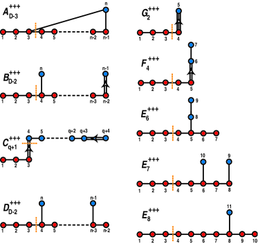
Figure 9.1: The nodes labelled 1,2,3 define the Kac–Moody extensions of the Lie algebras. The horizontal line starting at 1 defines the ‘gravity line’, which is the Dynkin diagram of a $A_{D-1}$ subalgebra.

The signatures found in the analysis of references [113, 114] and in the context of $S_{{\cal G}^{++}_{B}}$ in [69] match perfectly with the signature changing dualities and the exotic phases of M–theories discussed in [96, 97, 95].

In this context it is certainly interesting to extend to all ${\cal G}^{+++}$–theories the analysis of signature changing Weyl reflections. This is the purpose of the present chapter. We find for all the ${\cal G}^{++}_{B}$–theories all the possible signature $(T,S)$, where $T$ (resp. $S$) is the number of time–like (resp. space–like) directions, related by Weyl reflections of ${\cal G}^{++}$ to the signature $(1,D-1)$ associated to the theory corresponding to the traditional maximally oxidised theories. Along with the different signatures the signs of the kinetic terms of the relevant fields are also discussed. We start the analysis with $A_{D-3}^{++}$ corresponding to pure gravity in $D$ dimensions then we extend the analysis to the other ${\cal G}^{++}$, first to the simply laced ones and then to the non-simply laced ones. Each ${\cal G}^{++}$ algebra contains a $A_{D-3}^{++}$ subalgebra, the signatures of ${\cal G}^{++}$ should thus includes the one of $A_{D-3}^{++}$. This is indeed the case, but some ${\cal G}^{++}$ will contain additional signatures. If one want to restrict our focus on string theory, the special cases of $D_{24}^{++}$ and $B_{8}^{++}$ are interesting, the former being related to the low-energy effective action of the bosonic string (without tachyon) and the latter being related to the low-energy effective action of the heterotic string (restricted to one gauge field). The existence of signature changing dualities are related to the magnetic roots and suggests that these transformations correspond to a generalisation of the S–duality existing in these two theories [106, 161, 162].

9.1 The signatures of ${\cal G}^{++}_{B}$–theories

We will characterise the different signatures of ${\cal G}^{++}_{B}$ in terms of ${\cal G}^{+++}$, namely we will determine all the signatures in the Weyl orbit of $(1,D-1,\{\epsilon=+\})$ with the index 1 fixed to be a space–like coordinate. We first discuss in detail the ${\cal G}^{++}_{B}=A_{D-3}^{++}\subset A_{D-3}^{+++}$ case. The other ${\cal G}^{+++}$ contain as a subalgebra $A_{D-3}^{+++}$ (there is always a graviphoton present at some level) consequently the signatures of all ${\cal G}^{++}_{B}$ include at least those of $A_{D-3}^{++}$.

9.1.1 $A_{D-3}^{+++}$

$D>5$

Our purpose is to determine all $S_{{A}{}_{(i{}_{1}i{}_{2}\dots i{}_{t})}^{++}}^{(T,S,\varepsilon)}$ equivalent to $S_{A^{++}_{B}}$, i.e. all $\Omega^{\prime}$ related to $\Omega_{2}$ via a Weyl reflection of $A_{D-3}^{++}$ (see Eq.(6.18)). As explain above, the only Weyl reflections changing the signature in a non-trivial way are the ones generated by simple roots not belonging to the gravity line. Here there is only one such a simple root , namely $\alpha_{D}$ (see Figure 9.1). The Weyl reflection $W_{\alpha_{D}}$ exchanges the following roots,

$$\alpha_{D-1} \leftrightarrow \alpha_{D-1}+\alpha_{D}$$ (9.1)

$$\alpha_{3} \leftrightarrow \alpha_{3}+\alpha_{D}.$$ (9.2)

One can express this Weyl reflection as a conjugaison by a group element $U_{W_{\alpha_{D}}}$ of $A_{D-3}^{+++}$. The non-trivial action of $U_{W_{\alpha_{D}}}$, on the step operators is given by,

$$K^{D-1}{}_{D} \leftrightarrow \sigma R^{4...D,D-1}$$ (9.3)

$$K^{3}{}_{4} \leftrightarrow \rho R^{35...D,D},$$ (9.4)

where $\sigma$ and $\rho$ are +1 or -1 and the tensor $R^{a_{4}...a_{D},a_{D+1}}$ is in the representation $[1,0,\dots 1,0,0]$ of $A_{D-1}$ that occurs at level one [122]. $R^{4...D,D-1}$ is the generator of $A_{D-3}^{+++}$ associated to the root $\alpha_{D-1}+\alpha_{D}$ and $R^{35...D,D}$ the one associated to $\alpha_{3}+\alpha_{D}$.

In order to obtain a change of signature, we need generically $\Omega K^{3}{}_{4}\neq\Omega^{\prime}K^{3}{}_{4}$ and/or $\Omega K^{D-1}{}_{D}\neq\Omega^{\prime}K^{D-1}{}_{D}$. Using Eqs.(9.3), (9.4) and Eq.(6.20), these conditions are equivalent to $\mathrm{sign}(\Omega K^{3}{}_{4})\neq\mathrm{sign}(\Omega R^{35...D,D})$ and/or $\mathrm{sign}(\Omega K^{D-1}{}_{D})=\mathrm{sign}(\Omega R^{4...D,D-1})$. The following equalities,

$$\mathrm{sign}(\Omega R^{4...D,D}) = -\mathrm{sign}(\Omega R^{35...D,D}).\mathrm{sign}(\Omega K^{3}{}_{4})$$ (9.5)

$$= -\mathrm{sign}(\Omega R^{4...D,D-1}).\mathrm{sign}(\Omega K^{D-1}{}_{D}),$$

imply that we have only $\Omega K^{3}{}_{4}\neq\Omega^{\prime}K^{3}{}_{4}$ and $\Omega K^{D-1}{}_{D}\neq\Omega^{\prime}K^{D-1}{}_{D}$. These inequalities lead to four different possibilities summarised in Table 9.1.

Table 9.1: Conditions on $\Omega$’s leading to non-trivial signature changes under the Weyl reflection $W_{\alpha_{D}}$

	$\mathrm{sign}(\Omega K^{3}{}_{4}$)	$\mathrm{sign}(\Omega R^{35...D,D})$	$\mathrm{sign}(\Omega K^{D-1}{}_{D})$
a.	+	-	+
b.	+	-	-
c.	-	+	+
d.	-	+	-

Note that by Eq. (9.5) the sign of $\Omega R^{4...D,D-1}$ is deduced from the signs of $\Omega K^{3}{}_{4}$, $\Omega R^{35...D,D}$ and $\Omega K^{D-1}{}_{D}$. All the signatures in the orbit of $(1,D-1,+)$, where $+$ is the sign associated to the generator $R^{a_{4}...a_{D},a_{D+1}}$ defined by Eq.(6.21), are now derived.

• Step 1: Let us first consider a $\Omega$ characterised by a signature $(T,S,+)$ where $T$ is odd. We consider this set of signatures because it contains our starting point $(1,D-1,+)$ and also because other signatures of this type will be useful for the recurrence, i.e. the signature obtained from $(1,D-1,+)$ will lead in some cases to new signatures of the general type $(T,S,+)$ where $T$ is odd. We analyse the different possibilities of Table 9.1.

  • a. The coordinates $3$ and $4$ are of different nature as well as the coordinates $D-1$ and $D$. Moreover they are an even number of time coordinates in the set $\{3,5,...,D-1\}$ as a direct consequence of the sign $-$ in the second column of Table 9.1 and the fact that $R^{a_{4}...a_{D},a_{D+1}}$ satisfy Eq.(6.21) . So they are an odd number of time coordinates in the complementary subset $\{1,2,4,D\}$, i.e 1 or 3. These conditions lead to the possibilities given in Table 9.2.

    Table 9.2: $\Omega$’s leading to signature changes under the Weyl reflection $W_{\alpha_{D}}$. Space–like (resp. time–like) coordinate are denoted by s (resp. t)

    	1	2	3	4	…	D-1	D
    a.1.	s	t	t	s	…	t	s
    a.2.	s	s	s	t	…	t	s
    a.3.	s	s	t	s	…	s	t
    a.4.	s	t	s	t	…	s	t

    The nature of the coordinates 1, 2, 3 and $D$ (resp. 4,…,$D-1$) does not (resp. does) change under the action of the Weyl reflection generated by $\alpha_{D}$ on $\Omega$’s satisfying the conditions a given in Table 3. We must also determine which sign Eq.(6.21) or Eq.(6.22) characterises $R^{a_{1}...a_{D-3},a_{D-2}}$ under the action of the conjugated involution $\Omega^{\prime}$ given by Eq.(6.18). Using Eq.(6.23) one has $\mathrm{sign}(\Omega^{\prime}R^{4...D,D})=\mathrm{sign}(\Omega R^{4...D,D})=-1$ because there is an odd number of time coordinates in $\{4,...,D-1\}$ before Weyl reflection. The nature of all these coordinates changes under the action of $W_{\alpha_{D}}$. Therefore if $D$ is even, we have an odd number of time coordinates in this subset and $\mathrm{sign}(\Omega^{\prime}R^{4...D,D})$ satisfies Eq.(6.21). If $D$ is odd we get an even number of time coordinates yielding to the other sign Eq.(6.22). Therefore, the action of $W_{\alpha_{D}}$ on the $\Omega$’s characterised by the signatures of Table 9.2 yields $\Omega^{\prime}$’s characterised by the signatures given in Table 9.3.

    Table 9.3: $\Omega^{\prime}$’s obtained by the Weyl reflection $W_{\alpha_{D}}$ from $\Omega$’s given in Table 9.2

    	signature $\Omega^{\prime}$	conditions on $\Omega$
    a.1.	$(S,T,(-)^{D})$	$T\geq 3$ and $S\geq 3$
    a.2.	$(S-4,T+4,(-)^{D})$	$T\geq 3$ and $S\geq 4$
    a.3.	$(S,T,(-)^{D})$	$T\geq 3$ and $S\geq 4$
    a.4.	$(S,T,(-)^{D})$	$T\geq 3$ and $S\geq 3$

  • b. We get the same possibilities as those of case a (see Table 9.2) except for the coordinate $D-1$ which is different. Therefore the new signatures will be the same. Only the conditions on $S$ and $T$ can differ. These conditions are given in Table 9.4.

    Table 9.4: $\Omega^{\prime}$’s obtained by the Weyl reflection $W_{\alpha_{D}}$ from $\Omega$’s given in Table 9.2 with the nature of the coordinate $D-1$ changed

    	signature $\Omega^{\prime}$	conditions on $\Omega$
    b.1.	$(S,T,(-)^{D})$	$T\geq 3$ and $S\geq 4$
    b.2.	$(S-4,T+4,(-)^{D})$	$T\geq 1$ and $S\geq 5$
    b.3.	$(S,T,(-)^{D})$	$T\geq 3$ and $S\geq 3$
    b.4.	$(S,T,(-)^{D})$	$T\geq 5$ and $S\geq 2$

  • c. The coordinates $3$ and $4$ are of the same nature, $D-1$ and $D$ are of different nature. Moreover there are an odd number of time coordinates in $\{3,5,...,D-1\}$ and therefore an even number of time coordinates in the complementary subset $\{1,2,4,D\}$, i.e 0, 2 (1 being always space–like in ${\cal G}^{++}_{B}$). These conditions lead to the possibilities given in Table 9.5. The new signatures are given in Table 9.6 (the sign for $R^{a_{1}...a_{D-3},a_{D-4}}$ is determined by applying a similar reasoning as the one developed in case a).

    Table 9.5: $\Omega$’s leading to signature changes under the Weyl reflection $W_{\alpha_{D}}$ in case c. There is an odd number of time coordinates in the subset $\{4,...,D-1\}$

    	1	2	3	4	…	D-1	D
    c.1.	s	s	s	s	…	t	s
    c.2.	s	t	t	t	…	t	s
    c.3.	s	t	s	s	…	s	t
    c.4.	s	s	t	t	…	s	t

    Table 9.6: $\Omega^{\prime}$’s obtained by the Weyl reflection $W_{\alpha_{D}}$ from $\Omega$’s given in Table 9.5

    	signature $\Omega^{\prime}$	conditions on $\Omega$
    c.1.	$(S-4,T+4,(-)^{D})$	$T\geq 1$ and $S\geq 5$
    c.2.	$(S,T,(-)^{D})$	$T\geq 5$ and $S\geq 2$
    c.3.	$(S,T,(-)^{D})$	$T\geq 3$ and $S\geq 4$
    c.4.	$(S,T,(-)^{D})$	$T\geq 3$ and $S\geq 3$

  • d. We get the same signature as those of case c (see Table 9.5) except for the nature of the coordinate $D-1$. Again, only the conditions on $T$ and $S$ can differ. The new signatures are given in Table 9.7.

    Table 9.7: $\Omega^{\prime}$’s obtained by the Weyl reflection $W_{\alpha_{D}}$ from $\Omega$’s given in Table 9.5 with the nature of the coordinate $D-1$ changed

    	signature $\Omega^{\prime}$	conditions on $\Omega$
    d.1.	$(S-4,T+4,(-)^{D})$	$T\geq 1$ and $S\geq 6$
    d.2.	$(S,T,(-)^{D})$	$T\geq 3$ and $S\geq 3$
    d.3.	$(S,T,(-)^{D})$	$T\geq 3$ and $S\geq 3$
    d.4.	$(S,T,(-)^{D})$	$T\geq 5$ and $S\geq 2$

  Summary: From a signature $(T,S,+)$ with $T$ odd, we can reach the signatures

  $$(S-4,T+4,(-)^{D})\ \ \mathrm{if}\ \ \{\ T\geq 3\ \mathrm{and}\ S\geq 4\}\ \mathrm{or}\ \{T\geq 1\ \mathrm{and}\ S\geq 5\}$$

  $$(S,T,(-)^{D})\ \ \mathrm{if}\ \ \{T\geq 5\ \mathrm{and}\ S\geq 2\}\ \mathrm{or}\ \{T\geq 3\ \mathrm{and}\ S\geq 3\}.$$ (9.6)

  In order to find the Weyl orbits of $(1,D-1,+)$ we need to distinguish between $D$ even and $D$ odd.

  $D$ even: The conditions given by Eq. (9.6) simplify to

  $$(S-4,T+4,+)\ \ \mathrm{if}\ \ \{T\geq 1\ \mathrm{and}\ S\geq 5\}$$

  $$(S,T,+)\ \ \mathrm{if}\ \ \{T\geq 3\ \mathrm{and}\ S\geq 3\}.$$ (9.7)

  If we start from $(1,D-1,+)$, after the action of $W_{\alpha_{D}}$ one gets $(D-5,5,+)$ which is of the generic type $(T,S,+)$ with $T$ odd furthermore all the other signatures that we reach given by Eq.(9.7) are of this type. Therefore we can use the above analysis and taking into account the conditions Eq.(9.7) we conclude that when $D$ is even, the signatures in the $W_{\alpha_{D}}$ orbit of $(1,D-1,+)$ for ${\cal G}^{++}_{B}=A_{D-3}^{++}$ are given by ($n$ is an integer)

  $$(1,D-1,+)$$

  $$(1+4n,D-1-4n,+)\ 3\leq 4n+1\leq D-3$$

  $$(D-1-4n,1+4n,+)\ 5\leq 4n+1\leq D-1.$$ (9.8)

  $D$ odd: After the action of $W_{\alpha_{D}}$ the signature $(D-5,5,-)$ is not of the type $(T,S,+)$ with $T$ odd. To determine the orbit of $(1,D-1,+)$, we have thus to analyse the signatures of the form $(T,S,-)$ with $T$ even and $S$ odd.

• Step 2: Let us consider an involution $\Omega$ characterised by a signature $(T,S,-)$ where $T$ is even and $S$ is odd ($D$ is odd). The discussion of the different possible cases of signature change is similar to the ones discussed in step 1. Indeed, the even number of time coordinates balances the minus sign for the kinetic term of $R^{a_{1}...a_{D-3},a_{D-4}}$ (see Eq.(6.22)). We must be careful as far as the conditions on $T$ and $S$ are concerned. The only difference with the Tables 9.3, 9.4, 9.6, 9.7 is that we have for $D$ odd the opposite parity for the number of times in the coordinates $\{4,...,D-1\}$. Therefore, starting with $(T,S,-)$ we will reach the signature $(S,T,+)$ under the following conditions,

  $$(S,T,+)\ \ \mathrm{if}\ \ \{T\geq 2\ \mathrm{and}\ S\geq 5\}\ \mathrm{or}\ \{T\geq 4\ \mathrm{and}\ S\geq 3\}.$$ (9.9)

  The sign + given by Eq.(6.21) for $\Omega^{\prime}R^{a_{1}...a_{D-3},a_{D-4}}$ is obtained by a reasoning similar to the one given below Table 9.2 taking into account the fact that the number of dimensions is odd.

  The new signature Eq.(9.9) is of the type considered in step 1. The conditions for getting new signatures by acting again with $W_{\alpha_{D}}$ on this signature can thus be deduced from Eq.(9.6). Starting from $(1,D-1,+)$ the step 1 gives us $(D-5,5,-)$, then step 2 gives us $(5,D-5,+)$, step 1 can be used again to obtain $(D-9,9,-)$. Repeating the argument, all the new signatures are obtained using “step 1” or “step 2”.

  We conclude that when $D$ is odd, the following signatures can be reach,

  $$(1+4n,D-1-4n,+)\ 1\leq 4n+1\leq D-2$$

  $$(D-1-4n,1+4n,-)\ 1<4n+1\leq D.$$ (9.10)

We can rewrite Eq.(9.8) and Eq.(9.10) in a more concise way and conclude that for all $D$ (odd and even) the signatures of ${\cal G}^{++}_{B}$ in the Weyl orbit of $(1,D-1,+)$ are given by

$$(1+4n,D-1-4n,+)\ 0\leq n\leq[\frac{D-3}{4}]$$

$$(D-1-4n,1+4n,(-)^{D})\ 1<n\leq[\frac{D-1}{4}],$$ (9.11)

where $n$ is an integer and $[x]$ is the integer part of $x$.

$D=5$

The reasoning of the previous section cannot apply for $D=5$ because the conditions on $\Omega$ to obtain new signatures $\Omega^{\prime}$ given in Table 9.1 assumed $4<D-1$. These conditions give in this case $\mathrm{sign}(\Omega K^{3}{}_{4})\neq\mathrm{sign}(\Omega R^{35,5})$ and $\mathrm{sign}(\Omega K^{4}{}_{5})\neq\mathrm{sign}(\Omega R^{45,4})$. Starting from a signature $(1,4,+)$, this implies that the coordinate 4 must be the time. We get by acting with the Weyl reflection generated by $\alpha_{5}$ the signature $(0,5,-)$. Consequently all the possible signatures for $D=5$ are

$$(1,4,+)\ (0,5,-).$$ (9.12)

$D=4$

The Dynkin diagram of $A_{1}^{+++}$ is depicted in Fig.9.2.

Figure 9.2: Dynkin diagram of $A_{1}^{+++}$

To get a signature change due to the action of the Weyl reflection generated by $\alpha_{4}$ we need sign($\Omega K^{3}{}_{4}$) $\neq$ sign($\Omega R^{3,4}$) which is not possible since we started from $(1,3,+)$. The symmetric tensor $R^{a,b}$ is the representation [2,0,0] of $A_{3}$ that occurs at level one. The only possible signature is the Minkowskian one,

$$(1,3,+).$$ (9.13)

9.1.2 $D_{D-2}^{+++}$

$D>6$

They are two simple roots not belonging to the gravity line, namely $\alpha_{D}$ and $\alpha_{D+1}$ (see Figure 9.1). Given a signature $(T,S,\varepsilon)$, the first sign in the set $\varepsilon$ is associated to the generator $R^{a_{1}a_{2}}$ and the second one to the generator $R^{a_{5}...a_{D}}$ (see Eqs. (6.21) and (6.22)). We will analyse the possible signature changes due to $W_{\alpha_{D}}$ and $W_{\alpha_{D+1}}$.

1) The Weyl reflection generated by the root $\alpha_{D}$ will never non trivially change the signature. Indeed, its action on the simple root $\alpha_{D-2}$ and the corresponding action of $U_{W_{\alpha_{D}}}$ on the simple generator $R^{D-2\,D}$ are,

$W_{D}$:

$\alpha_{D-2}$

$\leftrightarrow$

$\alpha_{D-2}+\alpha_{D}$

$U_{W_{D}}$:

$K^{D-2}{}_{D-1}$

$\leftrightarrow$

$\sigma R^{D-2D}.$

Therefore to obtain a change of signature one needs (see Eq.(6.18)): $\mathrm{sign}(\Omega K^{D-2}{}_{D-1})\neq\mathrm{sign}(\Omega R^{D-2D})$. We have

$$\mathrm{sign}(\Omega R^{D-1D})=-\mathrm{sign}(\Omega R^{D-2D}).\mathrm{sign}(\Omega K^{D-2}{}_{D-1}),$$

thus $\mathrm{sign}(\Omega R^{D-1D})=+$ implies that the coordinates $D-1$ and $D$ are of different nature because $R^{D-1\,D}$ satisfies Eq.(6.21). So even if $\Omega^{\prime}K^{D-2}{}_{D-1}\neq\Omega K^{D-2}{}_{D-1}$ we will not have a non trivial signature change but just an exchange between the nature of the coordinates $D-1$ and $D$.

2) We now consider the action of the Weyl reflection generated by the root $\alpha_{D+1}$. Its action on $\alpha_{4}$ is

$W_{D+1}$:

$\alpha_{4}$

$\leftrightarrow$

$\alpha_{4}+\alpha_{D+1}$

$U_{W_{D+1}}$:

$K^{4}{}_{5}$

$\leftrightarrow$

$\rho R^{46...D}.$

In order to have a signature change, we need sign($\Omega K^{4}{}_{5})\neq$ sign($\Omega R^{46...D})$. This leads to two possibilities explicitly given in Table 9.8. The condition A means that the nature of the coordinates 4 and 5 are different and that if we start from $(T,S,\pm,+)$ (resp. $(T,S,\pm,-)$) there is an even (resp. odd) number of times in $\{4,6,...,D\}$ . Whereas condition B means that that the nature of the coordinates 4 and 5 are the same and that if we start from $(T,S,\pm,+)$ (resp. $(T,S,\pm,-)$) there is an odd (resp. even) number of times in $\{4,6,...,D\}$.

Table 9.8: Conditions on $\Omega$’s leading to non-trivial signature change under the Weyl reflection $W_{\alpha_{D}}$ for $S_{D_{D-2}^{++}}$

	sign($\Omega K^{4}{}_{5}$)	sign($\Omega R^{46...D}$)
A	+	-
B	-	+

• By analogy with the $A_{D-3}^{+++}$ case, we start from the signature $(T,S,+,+)$ where $T$ is an odd number.

  A. There is an odd number of times in $\{1,2,3,5\}$, i.e 1 or 3. These time coordinates can be distributed as in Table 9.9. The new signatures $\Omega^{\prime}$, also given in Table 9.9, are deduced from the fact that the action of the Weyl reflection generated by $\alpha_{D+1}$ will change the nature of the coordinates greater than 4.

  Table 9.9: $\Omega$’s leading to signature changes under the Weyl reflection $W_{\alpha_{D+1}}$ and the related new signatures $\Omega^{\prime}$’s (in the case A).

  	1	2	3	4	5	$\Omega^{\prime}$	$T\geq$	$S\geq$
  i.	s	s	t	t	s	$(S,T,+,(-)^{D})$	3	3
  ii.	s	s	s	s	t	$(S-4,T+4,+,(-)^{D})$	1	4
  iii.	s	t	t	s	t	$(S,T,+,(-)^{D})$	3	2

  B. There is an even number of times in $\{1,2,3,5\}$ i.e 0, 2 or 4. 4 is excluded here because we want that 1 is space–like. These time coordinates can be distributed as in Table 9.10. The new signatures are also given in Table 9.10.

  Table 9.10: $\Omega$’s leading to signature changes under the Weyl reflection $W_{\alpha_{D+1}}$ and the related new signatures $\Omega^{\prime}$’s (in the case B).

  	1	2	3	4	5	$\Omega^{\prime}$	$T\geq$	$S\geq$
  i.	s	s	s	s	s	$(S-4,T+4,+,(-)^{D})$	1	5
  ii.	s	s	t	t	t	$(S,T,+,(-)^{D})$	3	2
  iii.	s	t	t	s	s	$(S,T,+,(-)^{D})$	3	3

  $\Rightarrow$ if $D$ is even, from a signature $(T,S,+,+)$ we can reach the signatures $(S,T,+,+)$ (if $T\geq 3$ and $S\geq 3$) and $(S-4,T+4,+,+)$ (if $T\geq 1$ and $S\geq 5$ ).

  $\Rightarrow$ if $D$ is odd, from a signature $(T,S,+,+)$ we can reach the signatures $(S,T,+,-)$ (if $T\geq 3$ and $S\geq 2$) and $(S-4,T+4,+,-)$ (if $T\geq 1$ and $S\geq 4$).

• From the signature $(T,S,+,-)$ where $T$ is an even number and $S$ odd ($D$ is odd). By the same procedure, we can conclude that the signatures $(S,T,+,+)$ can be reached (if $T\geq 2$ and $S\geq 3$) and the signatures $(S-4,T+4,+,+)$ (if $S\geq 5$).

Summary: We get the same signatures as the ones of pure gravity as expected since $W_{\alpha_{D}}$ does not change the signature and only $W_{\alpha_{D+1}}$ has a non-trivial action,

$$(1+4n,D-1-4n,+,+)\ 0\leq n\leq[\frac{D-3}{4}]$$

$$(D-1-4n,1+4n,+,(-)^{D})\ 1<n\leq[\frac{D-1}{4}],$$ (9.14)

where $[x]$ is the integer part of $x$. We could have acted with the Weyl reflection generated by the graviphoton lying at level $(1,1)$ instead of acting with $W_{\alpha_{D+1}}$ and we would have obtained the same results. The sign of the kinetic term of the graviphoton agrees with Eq.(9.11).

$D=6$

They are two simple roots out of the gravity line, namely $\alpha_{6}$ and $\alpha_{7}$ (see Figure 9.3).

Figure 9.3: Dynkin diagram of $D_{4}^{+++}$

Given a signature $(T,S,\varepsilon)$, the first sign in the set $\varepsilon$ is associated to the generator $R^{a_{1}a_{2}}$ and the second one to the generator $\tilde{R}^{a_{1}a_{2}}$.

We can immediately conclude that no signature changes are possible. Indeed the Weyl reflections generated by the two simple roots not belonging to the gravity line cannot change the signature in the same way as the Weyl reflection $W_{\alpha_{D}}$ cannot do it in the previous section.

9.1.3 $E_{6}^{+++}$

They are two simple roots not belonging to the gravity line, $\alpha_{8}$ and $\alpha_{9}$ (see Figure 9.1). The non trivial actions of the corresponding Weyl reflections $W_{8}$, $W_{9}$ are

$W_{8}$:	$\alpha_{5}$	$\leftrightarrow$	$\alpha_{5}+\alpha_{8}$	$U_{W_{8}}$:	$K^{5}{}_{6}$	$\leftrightarrow$	$\rho R^{578}$
	$\alpha_{9}$	$\leftrightarrow$	$\alpha_{9}+\alpha_{8}$		$R$	$\leftrightarrow$	$\sigma\tilde{R}^{678}$
$W_{9}$:	$\alpha_{8}$	$\leftrightarrow$	$\alpha_{8}+\alpha_{9}$	$U_{W_{9}}$:	$R^{678}$	$\leftrightarrow$	$\delta\tilde{R}^{678}$.

The tensor $R^{abc}$ is the representation $[0,0,1,0,0,0,0]$ of $A_{7}$ that occurs at level $(1,0)$, the tensor $R$ is the representation [0,0,0,0,0,0,0] of $A_{7}$ that occurs at level $(0,1)$ and $\tilde{R}^{abc}$ is the representation $[0,0,1,0,0,0,0]$ of $A_{7}$ that occurs at level $(1,1)$ [122]. The sign of the kinetic term of $\tilde{R}^{abc}$ can be deduced from the ones of $R^{abc}$ and $R$, it is the product of these two signs.

The Weyl reflection generated by $\alpha_{9}$ exchanges the signs of $R^{abc}$ and $\tilde{R}^{abc}$.

To obtain a signature change from $(1,7,+,+)$, we must act with the Weyl reflection generated by $\alpha_{8}$ and there must be an odd number of time coordinates in the following subset: 6,7,8. In all of this cases, the new signature is $(2,6,-,-)$. Now we can start from this new signature and act with the Weyl reflection generated by $\alpha_{9}$ to get the signature $(2,6,+,-)$ or with the one generated by $\alpha_{8}$ to get $(5,3,+,+)$. Acting again with the Weyl reflections generated by $\alpha_{8}$ (vertical arrows) and $\alpha_{9}$ (horizontal arrows) on these signatures, we can conclude that all the signatures are

$(1,7,+,+)$
$\downarrow$
$(2,6,-,-)$	$\rightarrow$	$(2,6,+,-)$
$\downarrow$		$\downarrow$
$(5,3,+,+)$		$(3,5,-,+)$
$\downarrow$		$\downarrow$
$(6,2,-,-)$	$\rightarrow$	$(6,2,+,-).$

Theses signatures are the expected ones from the gravity, i.e. $(1,7,+,+)$, $(3,5,-,+)$ and $(5,3,+,+)$, plus new ones.

9.1.4 $E_{7}^{+++}$

They are two simple roots not belonging to the gravity line, $\alpha_{9}$ and $\alpha_{10}$. The non trivial actions of the Weyl reflections $W_{9}$, $W_{10}$ are

$W_{9}$:	$\alpha_{8}$	$\leftrightarrow$	$\alpha_{8}+\alpha_{9}$	$U_{W_{9}}$:	$K^{8}{}_{9}$	$\leftrightarrow$	$\rho R^{8}$
$W_{10}$:	$\alpha_{6}$	$\leftrightarrow$	$\alpha_{6}+\alpha_{10}$	$U_{W_{10}}$:	$K^{6}{}_{7}$	$\leftrightarrow$	$\delta R^{689}.$

The tensor $R^{a}$ is the representation $[1,0,0,0,0,0,0,0]$ of $A_{8}$ that occurs at level $(1,0)$, the tensor $R^{abc}$ is the representation [0,0,1,0,0,0,0,0] of $A_{8}$ that occurs at level $(0,1)$.

The Weyl reflection generated by the root $\alpha_{9}$ will change the signature if $\mathrm{sign}(\Omega K^{8}{}_{9})\neq\mathrm{sign}(\Omega R^{8})$. The Weyl reflection generated by the root $\alpha_{10}$ will change the signature if $\mathrm{sign}(\Omega K^{6}{}_{7})\neq\mathrm{sign}(\Omega R^{689})$. With these rules we get the following signatures (a horizontal arrow represents the action of the Weyl reflection generated by $\alpha_{10}$ and a vertical one the action of the Weyl reflection generated by $\alpha_{9}$),

$(1,8,+,+)$	$\rightarrow$	$(2,7,-,-)$	$\rightarrow$	$(5,4,+,+)$	$\rightarrow$	$(6,3,-,-)$
$\downarrow$		$\downarrow$		$\downarrow$		$\downarrow$
$(0,9,-,-)$	$\rightarrow$	$(3,6,+,+)$	$\rightarrow$	$(4,5,-,-)$	$\rightarrow$	$(7,2,+,+).$

The signs in the above signatures refer to the kinetic terms of $R^{a}$ and $R^{abc}$ (see Eqs.(6.21) and (6.22)).

9.1.5 $E_{8}^{+++}$

The signatures are given in [69]. To be complete, we recall them here,

$$(1,10,+)\ \rightarrow\ (2,9,-)\ \rightarrow\ (5,6,+)\ \rightarrow(6,5,-)\ \rightarrow(9,2,+).$$ (9.15)

The sign refers to the sign of the kinetic term of $R^{abc}$ which is the representation [0,0,1,0,0,0,0,0,0,0] of $A_{10}$ that occurs at level 1.

9.2 Non simply laced algebras

9.2.1 $B_{D-2}^{+++}$

The only non trivial action of the Weyl reflection generated by the short root $\alpha_{D}$ is

$W_{D}$: $\alpha_{D-1}$

$\leftrightarrow$

$\alpha_{D-1}+2\alpha_{D}$

$U_{W_{D}}$: $K^{D-1}{}_{D}$

$\leftrightarrow$

$\sigma R^{D-1D}.$

The tensor $R^{ab}$ is the representation $[0,1,0,,\dots,0]$ of $A_{D-1}$ that occurs at level $(2,0)$ [122]. To get a signature change with this Weyl reflection we need $\mathrm{sign}(\Omega K^{D-1}{}_{D})\neq\mathrm{sign}(\Omega R^{D-1D})$ which is impossible since the sign of the kinetic term of $R^{ab}$ is given by Eq.(6.21).

We are therefore left with one simple long root, namely $\alpha_{D+1}$. The Weyl reflection $W_{\alpha_{D+1}}$ will clearly produce the same signature changes as $W_{\alpha_{D+1}}$ does for $D_{D-2}^{+++}$. Therefore all possible signatures are the ones found for $D_{D-2}^{+++}$, i.e the signatures of pure gravity.

$$(1+4n,D-1-4n,+,+)\ 0\leq n\leq[\frac{D-3}{4}]$$

$$(D-1-4n,1+4n,+,(-)^{D})\ 1<n\leq[\frac{D-1}{4}],$$ (9.16)

where $[x]$ is the integer part of $x$. The first sign refers to the kinetic term of $R^{a}$ and the second to the one of $R^{a_{5}...a_{D}}$. $R^{a}$ is the representation [1,0,…,0] of $A_{D-1}$ that occurs at level $(1,0)$ and $R^{a_{5}...a_{D}}$ the representation [0,…,0,1,0,0,0] that occurs at level (0,1) [122].

9.2.2 $C_{q+1}^{+++}$

Clearly, if the Weyl reflections associated to $\alpha_{4}$ and $\alpha_{5}$ do not change the signature, there will be no signature changes. Let us first have a look at $\alpha_{5}$,

$W_{5}$:	$\alpha_{4}$	$\leftrightarrow$	$\alpha_{4}+\alpha_{5}$	$U_{W_{5}}$:	$R^{4}$	$\leftrightarrow$	$\rho\tilde{R}^{4}$
	$\alpha_{6}$	$\leftrightarrow$	$\alpha_{6}+\alpha_{5}$		$\tilde{R}$	$\leftrightarrow$	$\sigma\tilde{\tilde{R}}.$

The tensor $R^{a}$ is the representation $[1,0,0]$ of $A_{3}$ that occurs at level $(1,0,...,0)$, the tensor $\tilde{R}^{a}$ is the representation [1,0,0] of $A_{3}$ that occurs at level $(1,1,0,...,0)$, the tensor $\tilde{R}$ is the representation $[0,0,0]$ of $A_{3}$ that occurs at level (0,0,1,0,…,0) and $\tilde{\tilde{R}}$ is the representation $[0,0,0]$ of $A_{3}$ that occurs at level $(0,1,1,0,...,0)$. Because we started with a signature where all the generators have the sign of their kinetic term positive, we will not reach new signatures (i.e. here meaning new signs for the kinetic term of $R^{a}$ or $\tilde{R}$) with this reflection.

Let us now look at $\alpha_{4}$,

$W_{4}$:	$\alpha_{5}$	$\leftrightarrow$	$\alpha_{4}+\alpha_{5}$	$U_{W_{4}}$:	$R$	$\leftrightarrow$	$\tilde{R}^{4}$
	$\alpha_{3}$	$\leftrightarrow$	$\alpha_{3}+2\alpha_{4}$		$K^{3}{}_{4}$	$\leftrightarrow$	$R^{34}.$

The tensor $R$ is the representation [0,0,0] of $A_{3}$ that occurs at level (0,1,0,…,0), $R^{ab}$ is the representation [0,1,0] of $A_{3}$ that occurs at level (2,0,…,0). To get a signature change we need $\Omega(K^{3}{}_{4})\neq\Omega(R^{34})$ which is impossible because we have Eq.(6.21) for $R^{34}$.

9.2.3 $F_{4}^{+++}$

There are two short simple roots not belonging to the gravity line, namely $\alpha_{6}$ and $\alpha_{7}$. The generators associated to these simple roots are given in Table 9.11 respectively at level (1,0) and (0,1) [122].

Table 9.11: Level decomposition of $F_{4}^{+++}$

$(l_{1},l_{2})$	$A_{5}$ weight	Tensor
(0,1)	[0,0,0,0,0]	$R$
(1,0)	[1,0,0,0,0]	$R^{a}$
(1,1)	[1,0,0,0,0]	$\tilde{R}^{a}$
(2,0)	[0,1,0,0,0]	$R^{ab}$

The non trivial action of the Weyl reflection $W_{\alpha_{6}}$ (and of the corresponding conjugaison by a group element $U_{W_{\alpha_{6}}}$) on the simple roots (and on the corresponding simple generators) are,

$W_{6}$:	$\alpha_{5}$	$\leftrightarrow$	$\alpha_{5}+2\alpha_{6}$	$U_{W_{6}}$:	$K^{5}{}_{6}$	$\leftrightarrow$	$R^{56}$
	$\alpha_{7}$	$\leftrightarrow$	$\alpha_{7}+\alpha_{6}$		$R$	$\leftrightarrow$	$\tilde{R}^{6}.$

$W_{\alpha_{6}}$ can not change the signature because it needs sign($\Omega K^{5}{}_{6})\neq$ sign$(\Omega R^{56}$) which is impossible since the sign of the kinetic term for $R^{ab}$ is always positive. Moreover $W_{\alpha_{6}}$ can neither change the sign of the kinetic term of $R$ because we start from a signature such that all kinetic terms are characterised by Eq.(6.21). The action of $W_{\alpha_{7}}$ on the simple roots is,

$W_{7}$:

$\alpha_{6}$

$\leftrightarrow$

$\alpha_{6}+\alpha_{7}$

$U_{W_{7}}$:

$R^{6}$

$\leftrightarrow$

$\tilde{R}^{6}.$

This reflection can only a priori change the sign of the kinetic term for $R^{a}$. This sign can change if sign($\Omega R^{6}$) $\neq$ sign($\Omega\tilde{R}^{6}$) which is impossible since we started from a signature with all the signs given by Eq.(6.21). Therefore the only possible signature is

$$(1,5,+,+),$$ (9.17)

where the first sign refers to $R^{a}$ and the second to $R$.

9.2.4 $G_{2}^{+++}$

There is only one simple root not belonging to the gravity line, namely $\alpha_{5}$.

Table 9.12: Level decomposition of $G_{2}^{+++}$

$l$	$A_{4}$ weight	Tensor
1	[1,0,0,0]	$R^{a}$
3	[1,1,0,0]	$\tilde{R}^{abc}$

The only non trivial action of the Weyl reflection generated by $\alpha_{5}$ on the simple roots is (see Table 13)

$W_{5}$:$\alpha_{4}$

$\leftrightarrow$

$\alpha_{4}+3\alpha_{5}$

$U_{W_{5}}$:

$K^{4}{}_{5}$

$\leftrightarrow$

$\tilde{R}^{455}.$

To get a signature change we need sign($\Omega K^{4}{}_{5}$) $\neq$ sign($\Omega(\tilde{R}^{455}$), i.e. 5 is a time coordinate (because we start with the sign of $\tilde{R}^{abc}$ given by Eq.(6.21)). The new signature is the euclidian one $(0,5,-)$. These are the only signatures we can reach in agreement with pure gravity in $D=5$,

$$(1,4,+)\ \ (0,5,-),$$ (9.18)

where the sign refers to the kinetic term of $R^{a}$.

Conclusion

This thesis deals with recent aspects in the investigation of the symmetry structure of gravity. First, we addressed questions within the framework of the Cosmological Billiards. The billiard picture is derived within General Relativity, in studying the dynamics of the gravitational field (and other fields) in the vicinity of a space–like singularity. Of course, a satisfactory study of the gravitational field in this regime would require the knowledge of a quantum theory of gravity. In the quest for such a theory, it is however natural to examine General Relativity close to the regime where it breaks down. Moreover, the symmetries exhibited in a classical analysis might be also symmetries of the full quantum theory, even if the BKL analysis breaks down. The study of Cosmological Billiards suggests that Kac–Moody algebras might play an important role in a more fundamental theory of gravity. This observation deserves a more in–depth analysis. In this perspective, we obtained the following results:

– Our study of homogeneous cosmologies confirms the restoration of chaos when non–diagonal elements of the metric are kept in $5\leq D\leq 10$ [55]. When considering particular initial conditions, we found some Lorentzian Kac–Moody subalgebras of the algebras relevant in the generic, i.e. non homogeneous, context. We stressed the importance of having a better understanding of the momentum constraints in the generic case since in the very particular case of some empty $D=4$ homogeneous cosmologies, the billiard shape might depend on a gauge choice [but the finiteness, or infiniteness, of the billiard volume is not affected by a gauge choice]. We hope that these simplified models could provide a laboratory for the proof of the BKL conjecture in the chaotic cases.

– The shape of the billiards contains rather “coarse–grained” information about gravitational theories: it is invariant under dimensional reduction, it is not sensitive to Chern–Simons terms and it does not depend on the complete field content of the theories. From the billiard shape, we were able to derive information about the oxidation endpoint of the $D=3$ cosets of non–split groups coupled to gravity [50]. More precisely, we gave the highest dimensions for all cases and showed how to find the field content of these oxidation endpoints.

– We next turned to hyperbolic Kac–Moody algebras. These algebras are of particular interest since they characterise chaotic Kac–Moody billiards. For any Kac–Moody algebra, we addressed the questions of the existence of a Lagrangian reproducing this algebra and the maximal dimension in which such a Lagrangian exists. We completely answered these questions and gave explicitly the minimal field content of the Lagrangians in the highest dimensions [56]. The maximal rank for hyperbolic algebras is 10 (and only four hyperbolic algebras do exist); we confirmed the oxidation endpoint for $CE_{10}$ (spacetime dimension, field content and Lagrangian) that is the only rank 10 hyperbolic algebra a priori not related to a string/M–theories. Our analysis restricts to the Weyl groups of hyperbolic algebras, but the search for Lagrangians invariant under these algebras [which are not over–extended algebras] has not been considered. Non–linear realisations based on these algebras might give a hint on how to handle this problem.

As stated above, one of most attractive features of Cosmological Billiards lies in the beautiful symmetric structure of gravitational theories they reveal and which is believed to be preserved in a quantum regime, although the BKL behaviour might be destroyed. Attempts to make this symmetry manifest and to go beyond this billiard picture have been suggested by the construction of actions invariant under Kac–Moody algebras. Reference [43] proposed an action invariant under $E_{8(8)}^{++}$ —which is the case relevant to $D=11$ supergravity— that describes a geodesic motion on the coset space $E_{8(8)}^{++}/K(E_{8(8)}^{++})$. The equations of motion resulting from this action have been compared, level by level, to the equations of motion of the (bosonic sector of the) $D=11$ supergravity. The matching is perfect up to level $3^{-}$ or equivalently height 30 (which is much better than the height 1 roots accessed in the billiard picture). The inclusion of fermions was however lacking in this construction but we filled this gap in [52]. In the meanwhile, we showed that:

– The Dirac field is compatible with the hidden symmetries that emerge upon toroidal dimensional reduction to three dimensions, provided one appropriately fixes its Pauli couplings to the $p$–forms [51]. We have only considered the split real form for the symmetry (duality) group in three dimensions, but similar conclusions would apply to the non–split forms. We have also indicated that the symmetry considerations reproduce some well known features of supersymmetry when supersymmetry is available.

– The Dirac field is compatible with the conjectured infinite–dimensional symmetry ${\cal G}^{++}$ and a perfect matching was found with the non–linear $\sigma$–model equations minimally coupled to a $(1+0)$ Dirac field, up to the levels where the bosonic matching works [51].

– The Dirac fermions get frozen à la limite BKL. Moreover when the fermionic currents are treated as ordinary classical fields, chaos will be destroyed —whenever it is present in the bosonic theory— in agreement with the findings of [8]. A direct group theoretical interpretation of this result is that the motion in the Cartan subalgebra becomes time–like [51].

– The gravitino field of 11–dimensional supergravity is compatible with the conjectured hidden $E_{10(10)}$ symmetry up to the level reached in the bosonic sector. In $\sigma$–model terms, the supergravity action is given by the (first terms of the) action for a spinning particle on the symmetric space $E_{10(10)}/K(E_{10(10)})$, with the internal degrees of freedom in the ‘spin 3/2’ representation of $K(E_{10(10)})$ (modulo the 4–fermion terms) [52]. This action takes the same form as the action for a Dirac spinor but with the appropriate ‘spin 3/2’ representation. We can thus analyse its dynamics in terms of the conserved $K(E_{10(10)})$ currents along the same lines as for the spin 1/2 case and conclude that the BKL limit holds. We have treated explicitly the case of $D=11$ supergravity, but a similar analysis applies to the other supergravities, described also by infinite–dimensional Kac–Moody algebras (sometimes in non–split forms [89, 78]). The inclusion of fermions in the ${\cal G}^{+++}$–invariant actions could be considered along the same lines.

Actions invariant under ${\cal G}^{+++}$ have been proposed in [71] that encompass two non equivalent actions invariant under ${\cal G}^{++}$, $S_{{\cal G}^{++}_{B}}$ and $S_{{\cal G}^{++}_{C}}$ [69]. The action $S_{E_{8(8)\,B}^{++}}$ has been shown to possess “extremal brane” solutions that form orbits under the Weyl group identifiable with the U–duality orbits existing in M–theory [71, 72]. This strongly suggests a general group–theoretical origin of ‘dualities’ for all $S_{{\cal G}^{++}_{B}}$ –theories transcending string theories and supersymmetry [71, 72, 73]. One aspect of the dualities is that they can change the spacetime signature [96, 97, 95]. In this context, we extended to all $S_{{\cal G}^{++}_{B}}$–theories the analysis of signature changing Weyl reflections [53]. We found for all the $S_{{\cal G}^{++}_{B}}$–theories all the possible signatures $(T,S)$ —where $T$ (resp. $S$) denotes the number of time–like (resp. space–like) directions— related by Weyl reflections of ${\cal G}^{++}$ to the Lorentzian $(1,D-1)$ signature. Along with the different signatures the signs of the kinetic terms of the relevant fields have been discussed. In the context of string theory, the special cases of $D_{24}^{++}$ and $B_{8}^{++}$ are interesting.

The attempts to reformulate “M–theories” as non–linear realisations are very instructive. They do not include space(time) as a basic ingredient, rather it is hoped to be encoded in the dynamics. To understand how, a proof of the conjecture that certain infinite “tower” of representations encode the spatial derivatives the (supergravity) fields [43] would be illuminating. But it seems that a better knowledge of Kac–Moody algebras is needed to tackle this statement. A first step in this direction could be to seek solutions to the Kac–Moody invariant actions that are identifiable as supergravity solutions that depend on two spacetime coordinates. A better understanding of infinite–dimensional subalgebras might be of great important in that context. More generally, difficulties arise in the interpretation of fields of increasing level (for instance, for $E_{10(10)}$, no dictionary has been established for fields of level $\ell>3^{-}$). Various interesting propositions have been put forward for how to understand the structure of these higher level fields. First, the conjecture mentioned above about the spatial derivatives. Furthermore, these higher level fields may also be interpreted as candidates for higher spin fields because of their index structure (see for instance [54] and references therein). Recently, some very promising results have also been obtained regarding the incorporation of quantum corrections into the structure of the Kac–Moody algebras related to string and M–theory [48, 125, 38]. More precisely, for M–theory the leading contribution of the 8th derivative correction is associated with the fundamental weight $\Lambda_{10}$ conjugate to the exceptional simple root of $\mathfrak{e}_{10(10)}$. Subdominant terms at the same order in derivatives then contributes by the addition of positive roots to this weight. This opens up the tantalising possibility that M–theoretical corrections are encoded in (non–integrable) representations of $e_{10(10)}$. Since the dominant weights, appearing as lowest weights in the representations, correspond to negative levels these results indicate that the original $E_{10(10)}$–invariant action [based on a Borel–type decomposition] is probably insufficient to incorporate the full structure of M–theory. Reference [19] also deals with imaginary roots.

Whatever M–theory will be, we believe that it will reflect the deep connections between dimensional reduction, asymptotic dynamics of the gravitational field in the vicinity of a space–like singularity, hidden symmetries, dualities, non–local transformations and infinite–dimensional Lie algebras.

Appendix A Simple Lie Algebras

This appendix is based on [79] and [99]. For more details and examples, see [16].

A.1 Structure of Simple Lie Algebras

Basic Definitions

A complex Lie algebra ${\mathfrak{g}}$ is a vector space equipped with a binary operation $[\ ,\ ]$ called a commutator, mapping ${\mathfrak{g}}\times{\mathfrak{g}}$ into ${\mathfrak{g}}$ with the following properties; $\forall\ x,y,z\ \in{\mathfrak{g}}$ and $\forall\ \alpha,\beta\in\mathbb{C}$,

$$1. \mathrm{Antisymmetry}:[x,y]=-[y,x]\,;$$

$$2. \mathrm{Bilinearity}:[\alpha x+\beta y,z]=\alpha[x,z]+\beta[y,z]\,;$$

$$3. \mathrm{Jacobi\ identity}:[[x,y],z]+[z,[x,y]]+[y,[z,x]]=0\,.$$

A Lie algebra $\mathfrak{g}$ can be specified by a set of generators $\{J^{b}\}$ and their commutations relations

$$[J^{b},J^{c}]=f^{bc}_{\hskip 8.5359ptd}J^{d}\,.$$

The dimension of the algebra is the dimension of the underlying vector space. The constants $f^{bc}_{\hskip 8.5359ptd}$ are the structure constants.

Simple Lie algebras are non-abelian Lie algebras that contain no proper ideal. An ideal $\mathfrak{i}$ of ${\mathfrak{g}}$ is a subspace of ${\mathfrak{g}}$ such that $\ [\mathfrak{i},\mathfrak{g}]\subset\mathfrak{i}\,$.

Semi-simple Lie algebras are Lie algebras that contain no abelian ideal and that are not empty. Every semi-simple Lie algebra can be decomposed into the direct sum of its simple ideals (see theorem in Section 5.2 of [99]).

Levi theorem: Every Lie algebra can be decomposed into the direct sum of simple Lie algebras and solvable algebras (a solvable algebra is a Lie algebra such that the series $\ L^{(0)}=L,\ L^{(1)}=[L^{(0)},L^{(0)}],\ L^{(k)}=[L^{(k-1)},L^{(k-1)}]$ stops for some $k$).

A linear representation $\Gamma$ of a Lie algebra ${\mathfrak{g}}$ in the vector space $V$ is an homomorphism

$$\Gamma:\ {\mathfrak{g}}\rightarrow\mathfrak{gl}(V):x\rightarrow\Gamma(x)\,,\quad\Gamma(x):V\rightarrow V:v\rightarrow\Gamma(x)\cdot v\,.$$ (A.1)

The linear operator $\Gamma(x)$ is sometimes simply denoted by $x\,$.

The Cartan-Weyl Basis and Roots

Only semi-simple complex Lie algebras are treated. In the Cartan-Weyl basis, the generators are constructed as follows. We first find the maximal set of commuting generators $H^{i}\,$, $i=1,...,r\,$, such that $ad_{H^{i}}$ is semi-simple for all $i$ (an endomorphism is called semi-simple if in a suitable basis it can be expressed by means of a diagonal matrix). This set of operators forms the Cartan subalgebra $\mathfrak{g}_{\circ}$. The rank of $\mathfrak{g}$ is defined to be the dimension $r$ of its Cartan subalgebra.

Because the matrices $ad_{H^{i}}$ can be simultaneously diagonalized, the remaining generators are chosen to be those particular combinations $E^{\alpha}$ of the $J^{a}$’s that satisfy the following eigenvalue equations

$$ad_{H^{i}}E^{\alpha}=[H^{i},E^{\alpha}]=\alpha(H^{i})E^{\alpha}$$

where the $\alpha(H^{i})$, also noted $\alpha^{i}$, are the (not all vanishing) components of elements of $\mathfrak{g}_{\circ}^{\star}$, the dual of the Cartan subalgebra $\mathfrak{g}_{\circ}\,$. The non-zero elements $\alpha$ of $\mathfrak{g}_{\circ}^{\star}$ such that the set

$${\mathfrak{g}}_{\alpha}=\{~{}X\in{\mathfrak{g}}~{}~{}\arrowvert~{}~{}[H^{i},X]=\alpha^{i}\,X~{}~{}~{}\forall~{}H^{i}\in\mathfrak{g}_{\circ}\ \}$$

is not empty are called roots. The set of all roots of $\mathfrak{g}$ is denoted $\Delta$ and is called the root system of $\mathfrak{g}$. $E^{\alpha}$ is the corresponding ladder operator. To get the commutation relations between the ladder operators, one observes that the Jacobi identity implies

$$\ [H^{i},[E^{\alpha},E^{\beta}]]=(\alpha^{i}+\beta^{i})[E^{\alpha},E^{\beta}]\ .$$

If $\alpha+\beta\ \in\ \Delta$, the commutator $\ [E^{\alpha},E^{\beta}]$ must be proportional to $E^{\alpha+\beta}$. It certainly must vanish if $\alpha+\beta$ is not a root. When $\alpha=-\beta$, the commutator $[E^{\alpha},E^{-\alpha}]$ commutes with all $H^{i}$, which is possible only if it is a linear combination of the generators of the Cartan subalgebra (see Eq.(A.18) for precise relation). Therefore, the full set of commutation relations in the Cartan-Weyl basis is

(A.9)

The Killing Form and Properties of Roots

In order to know the Cartan-Weyl basis more explicitly, more must be said about the root system $\Delta$. The Killing form plays an important role in this perspective.

A bilinear and symmetric form on $\mathfrak{g}$, called the Killing form, can be defined by

$K(x,y):=\mathrm{tr}(\mathrm{ad}_{x}\ \mathrm{ad}_{y})\hskip 42.67912pt\forall x,\ y\in{\mathfrak{g}}$ .

The Killing form possesses important properties: (i) its invariance (under the adjoint action) $K(x,[y,z])=K([x,y],z)~{}~{}\forall~{}x,y,z\in{\mathfrak{g}}$; (ii) it is non-degenerate (Cartan’s criterion); (iii) the restriction of the Killing form to $\mathfrak{g}_{\circ}$ is non-degenerate.

The fundamental role of the Killing form is to establish an isomorphism between $\mathfrak{g}_{\circ}$ and $\mathfrak{g}_{\circ}^{\star}\,$. To every $\gamma\in\mathfrak{g}_{\circ}^{\star}$ corresponds, up to a normalization factor $c_{\gamma}$, an element $H^{\gamma}\in\mathfrak{g}_{\circ}$ through

$$\gamma(h)=c_{\gamma}K(h,H^{\gamma})\hskip 28.45274pt\forall\;h\in\mathfrak{g}_{\circ}\,.$$ (A.10)

To avoid the normalization factor, we also define $h_{\gamma}:=c_{\gamma}H^{\gamma}\,$. With this isomorphism, the Killing form can be transferred into a (non-degenerate) inner product on $\mathfrak{g}_{\circ}^{\star}\,$:

(A.14)

Using the Killing form, the commutation relation between $E^{\alpha}$ and $E^{-\alpha}$ can be established. One can show that,

(A.18)

Here are listed some important results concerning the root system $\Delta$ of (finite-dimensional) semi-simple complex Lie algebras.

• The roots span all $\mathfrak{g}_{\circ}^{\star}\,$: span${}_{\mathbb{C}}(\Delta)=\mathfrak{g}_{\circ}^{\star}\,$

• The root spaces $\mathfrak{g}_{\alpha}$ are one-dimensional ($\mathfrak{g}_{\alpha}=$ span${}_{\mathbb{C}}\{E^{\alpha}\}$), i.e. the roots are non-degenerate;

• The only multiples of $\alpha\in\Delta$ which also belong to $\Delta$ are $\pm\alpha\;$;

• On $\mathfrak{g}_{\circ}(\mathbb{R})$, the real vector space with basis $\{H^{i}\}_{i=1}^{r}$ (or $\{h_{\beta_{i}}\}_{i=1}^{r}$), we have $\alpha(H^{i})\in\mathbb{R}$ $\;\forall\;i$ and $\forall\;\alpha\in\Delta$.

• $K(h,h^{\prime})$ is real for all $h$, $h^{\prime}\in\mathfrak{g}_{\circ({\mathbb{R}})}$. Moreover, for all $h\in\mathfrak{g}_{\circ}(\mathbb{R})$, $K(h,h)\geqslant 0$ and $K(h,h)=0$ implies $h=0$.

The Killing form thus provides an Euclidean metric on the root space $\mathfrak{g}^{\star}_{\circ}(\mathbb{R})$, so that we have $\mathfrak{g}^{\star}_{\circ}(\mathbb{R})\cong\mathbb{R}^{\mbox{r}}$. This highly non-trivial fact is one of the key ingredients in the classification of all finite-dimensional simple Lie algebras.

Simple Roots, Cartan Matrix and Dynkin Diagram

Let $h_{\beta_{1}}$, $h_{\beta_{2}}$, $\ldots h_{\beta_{r}}$ be a set of $r$ linearly independent elements of $\mathfrak{g}_{\circ}$, where $\beta_{i}\in\Delta$, $1\leqslant i\leqslant r\,$. It can be shown that every non-zero root $\alpha$ of $\Delta$ can be written in the form $\alpha=\sum_{j=1}^{r}k_{i}\beta_{j}\,,\quad k_{i}\in\mathbb{Q}\,,\quad i=1,\ldots,r$. A non-zero root of $\Delta$ is said to be positive (with respect to this basis) if the first non-vanishing coefficient of the set $\{k_{i}\}_{i=1}^{r}$ is positive. One then writes $\alpha>0$. The set of all positive (resp. negative) roots is denoted $\Delta_{+}$ (resp. $\Delta_{-}$). A simple root is a positive root that cannot be written as the sum of two positive roots. If ${\mathfrak{g}}$ has rank $r$ then ${\mathfrak{g}}$ possesses precisely $r$ simple roots $\{\alpha^{(i)}\}_{i=1}^{r}$. They form a basis of the dual space $\mathfrak{g}_{\circ}^{\star}\,$ such that every positive root $\alpha$ can be written as $\alpha=\sum_{i=1}^{r}k_{i}\alpha^{(i)}\in\Delta_{+}$ where the $k_{i}$’s are non negative integers. The level or height of $\alpha$ is the positive integer $k=\sum_{i=1}^{r}k_{i}\,$.

A lexicographic ordering of roots can be introduced: let $\alpha$ and $\beta$ be any two roots of $\Delta\,$, then if $\alpha-\beta$ is positive, $(\alpha-\beta)>0\,$, one writes $\alpha>\beta\,$.

The Cartan matrix $\mathbf{A}$ of ${\mathfrak{g}}$ is an $r\times r$ matrix whose elements $A^{ij}$ are defined in terms of the simple roots $\{\alpha^{(i)}\}_{i=1}^{r}$ of ${\mathfrak{g}}$ by

(A.22)

The Cartan matrix A possesses the following properties: $A^{ii}=2$ $\forall$ $i\in\{1,\ldots,r\}$; for $i\neq j$ the only possible values of $A^{ij}$ are $0$, $-1$, $-2$ or $-3$; $A^{ij}=0$ if and only if $A^{ji}=0\,$.

The coroot of the simple root $\alpha^{(i)}$ is

$$\alpha^{(i)\vee}:={2\alpha^{(i)}\over(\alpha^{(i)},\alpha^{(i)})}\,.$$

There is a highest root $\Theta$, the unique root for which, in the expansion $\sum m_{i}\alpha^{(i)}$, the height (or level) $\sum m_{i}$ is maximized.

One depicts a so-called Dynkin diagram for each simple complex Lie-algebra ${\mathfrak{g}}$ where each simple root $\alpha^{(i)}$ of ${\mathfrak{g}}$ is assigned a point (a vertex) and max$\{|A^{ij}|,|A^{ji}|\}$ lines are drawn between the vertices corresponding to $\alpha^{(i)}$ and $\alpha^{(j)}$ with an arrow towards the shortest root, i.e. if $\sqrt{\alpha_{(i)},\alpha_{(i)}}<\sqrt{\alpha_{(j)},\alpha_{(j)}}$ the arrow is directed toward $\alpha_{(i)}$.

Remaining Commutation Relations

If $\alpha,\ \beta,\ \gamma,\ \delta,\ \alpha+\beta\in\Delta$, and $p,\ q$ are such that the $\alpha$-string containing $\beta$ is $\beta-p\,\alpha$, $\ldots$, $\beta$, $\ldots$, $\beta+q\,\alpha$ it can be shown that the $N_{\alpha,\beta}$’s of Eq.(A.9) are such that

• $N_{\alpha,\beta}\neq 0\,$ ;

• $N_{\beta,\alpha}=-N_{\alpha,\beta}$ ;

• if $\alpha+\beta+\gamma=0$, $N_{\alpha,\beta}K_{\gamma}=N_{\beta,\gamma}K_{\alpha}=N_{\gamma,\alpha}K_{\beta}$ where $K_{\alpha}=K(E^{\alpha},E^{-\alpha})$;

• if $\alpha,\,\beta,\,\gamma,\,\delta$ are such that the sum of two of them is never zero, and if $\alpha+\beta+\gamma+\delta=0$, then $N_{\alpha,\beta}N_{\gamma,\delta}K_{\alpha+\beta}+N_{\beta,\gamma}N_{\alpha,\delta}K_{\beta+\gamma}+N_{\gamma,\alpha}N_{\beta,\delta}K_{\alpha+\gamma}=0$

• $N_{\alpha,\beta}N_{-\alpha,-\beta}=-\frac{1}{2}(\alpha,\alpha)\frac{K_{\alpha}K_{\beta}}{K_{\alpha+\beta}}q(p+1)$;

• with $K(E^{\alpha},E^{-\alpha})$ taking any assigned value $K_{\alpha}$ for each pair of roots $\alpha$, $-\alpha\in\Delta$, the basis elements of ${\mathfrak{g}}$ may be chosen so that either $N_{\alpha,\beta}=N_{-\alpha,-\beta}$ $\forall$ $\alpha$, $\beta$ $\in\Delta$ or $N_{\alpha,\beta}=-N_{-\alpha,-\beta}$ $\forall$ $\alpha$, $\beta$ $\in\Delta$.

To fix the commutations relations (A.9, A.18) up to signs, one can for instance take

1. $K_{\alpha}=1\ \forall\ \alpha\in\Delta$ (one denotes the ladder operators normalised accordingly by $e_{\alpha}$) and
2. $N_{-\alpha,-\beta}=-N_{\alpha,\beta}\ \forall\alpha,\beta\ \in\Delta$. With these conventions, all $N_{\alpha,\beta}$ are real and obey

$$N_{\alpha,\beta}{}^{2}={1\over 2}(\alpha,\alpha)q(p+1)\ .$$

3. Moreover, one chooses the Cartan generators chosen to be the $h_{\alpha}$ such that $\alpha(h)=K(h,h_{\alpha})\ \forall\ h\in\mathfrak{g}_{\circ}$.

With these normalisations, the commutation relations write

$$\ [h_{\alpha},h_{\beta}] = 0\ ,$$

$$\ [h_{\alpha},e_{\beta}] = \beta(h_{\alpha})e_{\beta}\ ,$$

$$\ [e_{\alpha},e_{\beta}] = \pm\sqrt{{1\over 2}(\alpha,\alpha)q(p+1)}e_{\alpha+\beta}\ \ \ \mathrm{if}\ \alpha+\beta\in\Delta\ ,$$ (A.23)

$$= h_{\alpha}\ \ \hskip 102.43008pt\mathrm{if}\ \beta=-\alpha\ ,$$

$$= 0\ \ \hskip 108.12054pt\mathrm{ortherwise}\ .$$

Two other choices are often used in the literature, the Chevalley basis and the orthonormal basis.

The Chevalley Basis and Serre Relations

The Chevalley basis is a particular case of Cartan-Weyl basis which is the one most useful for studying representations. In this section, a construction of finite dimensional simple Lie algebras based on Cartan matrices and called the Chevalley–Serre construction is presented. A Cartan matrix $A\,$ is an $r\times r$ matrix such that (i) $A_{ii}=2$, (ii) $A_{ij}=0,-1,-2,-3$ for $i\neq j$, (iii) $A_{ij}=0\iff A_{ji}=0$ for $i\neq j$, (iv) det($A)>0$, (v) $A$ is indecomposable, i.e. there is no renumbering of the indices which would bring $A$ to a block diagonal form. Any finite dimensional simple Lie algebra $\mathfrak{g}(A)$ can be built out of a Cartan matrix $A$, see e.g. [99]. The algebra $\mathfrak{g}(A)$ is generated by 3 $r$, $\{e_{i},\,f_{i},\,h_{i}\}_{i=1,...,r}$ obeying the following commutation relations,

$[h^{i},h^{j}]$	$=\ 0\,,$
$[h^{i},e^{j}]$	$=\ A^{ji}e^{j}\,,$
$[h^{i},f^{j}]$	$=-\ A^{ji}f^{j}\,,$
$[e^{i},f^{j}]$	$=\ \delta^{ij}h^{i}\,.$

Moreover, their multi-commutators (the remaining generators) are subject to the so-called Serre relations,

$${(\mathrm{ad}_{e^{i}})}^{1-A^{ji}}e^{j} = 0\,,$$

$${(\mathrm{ad}_{f^{i}})}^{1-A^{ji}}f^{j} = 0\,.$$

It can be shown that the algebra $\mathfrak{g}(A)$ admits a triangular decomposition,

$$\mathfrak{g}(A)=n_{-}\oplus\mathfrak{g}_{\circ}\oplus n_{+}\,,$$

where $\mathfrak{g}_{\circ}$ is the Cartan subalgebra generated by the $h_{i}$, $n_{-}$ is nilpotent and generated by the multicommutators of the $f_{i}$ (elements of the form $\ [f_{i},[f_{j},[...,[f_{k},f_{l}]]]]$) and $n_{+}$ is generated by multicommutators of the $e_{i}$. As mentioned above, the roots are not degenerate therefore to each multicommutator $e_{\alpha}$ of the $e_{i}$ correspond one positive root $\alpha$ and to each multicommutator $f_{\alpha}$ of the $f_{i}$ correspond one negative root $-\alpha$.

This choice of basis corresponds to the following normalisation choices,

1. The $h^{i}$ are equal to the $H^{(\alpha^{i})}$ of Eq.(A.10) with $c_{\alpha^{i}}=(\alpha^{(i)},\alpha^{(i)})/2$, i.e. they are normalised such that the equation $\alpha^{(i)}(h)=1/2\ (\alpha^{(i)},\alpha^{(i)})K(h,h^{i})$ is satisfied.
2. The $e^{i}$ and $f^{i}$ are the previously introduced $E^{\alpha^{(i)}}$ and $E^{-\alpha^{(i)}}$ generators normalised such that $K_{\alpha^{(i)}}=K(E^{\alpha^{(i)}},E^{-\alpha^{(i)}})=2/(\alpha^{(i)},\alpha^{(i)})$. They obey Eq.(A.18) which, with these normalisations, rewrites $\ [e_{i},f_{i}]=h_{i}$.
3. The normalisation of the multicommutators $e_{\alpha}$ is chosen such that $K(e_{\alpha},f_{\alpha})=2/(\alpha,\alpha)$.

Remark : The Cartan-Chevalley involution $\tau$ reads

$$\tau(h_{i})=-h_{i},\hskip 28.45274pt\tau(e_{i})=-f_{i}\hskip 14.22636ptand\hskip 14.22636pt\tau(e_{\alpha})=(-1)^{ht(\alpha)}f_{\alpha}\,.$$ (A.24)

Chevalley Basis up to signs

A slightly different convention is the same as here above except that we take the “negative” generators $f_{i}$ with the opposite sign. The only relation that is modified is $[e_{i},f_{j}]=-\delta_{ij}\,h_{i}$. The sign convention for $f_{i}$ simplifies somewhat the form of the generators of the maximal compact subalgebra . The Cartan-Chevalley involution reads $\tau(h_{i})=-h_{i}$, $\tau(e_{i})=f_{i}$, $\tau(f_{i})=e_{i}$ and extends to the higher height root vectors as $\tau(e_{\alpha})=f_{\alpha}$, $\tau(f_{\alpha})=e_{\alpha}$. A basis of the maximal compact subalgebra is given by $k_{\alpha}=e_{\alpha}+f_{\alpha}$. It is convenient to define $g^{T}=-\tau(g)$ for any Lie algebra element $g$. The invariant bilinear form on the Lie algebra is given for the Chevalley-Serre generators by

$$K(h_{i},h_{j})=\frac{2\,A_{ji}}{(\alpha_{i}|\alpha_{i})}=\frac{2\,A_{ij}}{(\alpha_{j}|\alpha_{j})},\;\;K(h_{i},e_{j})=K(h_{i},f_{j})=0,\;\;K(e_{i},f_{j})=-\frac{2\delta_{ij}}{(\alpha_{i}|\alpha_{i})}$$ (A.25)

and is extended to the full algebra by using the invariance relation $K(x,[y,z])=K([x,y],z)$. Here, the $\alpha_{i}$’s are the simple roots. The induced bilinear form in root space is denoted by $(\cdot|\cdot)$ and given by $(\alpha_{i}|\alpha_{j})=\frac{2A_{ij}}{(\alpha_{i}|\alpha_{i})}$. The numbers $(\alpha_{i}|\alpha_{i})$ are such that the product $A_{ij}\,(\alpha_{i}|\alpha_{i})$ is symmetric and they are normalized so that the longest roots have squared length equal to $2$. One gets

$$K(h_{i},e_{\alpha})=K(h_{i},f_{\alpha})=0=K(e_{\alpha},e_{\beta})=K(f_{\alpha},f_{\beta}),\;\;K(e_{\alpha},f_{\beta})=-N_{\alpha}\delta_{\alpha\beta},$$ (A.26)

where the coefficient $N_{\alpha}$ in front of $\delta_{\alpha\beta}$ in the last relation depends on the Cartan matrix (and on the precise normalization of the root vectors corresponding to higher roots – e.g., $N_{\alpha}=\frac{2}{(\alpha|\alpha)}$ in the Cartan-Weyl-Chevalley basis).

Orthonormal Basis

The Killing form of ${\mathfrak{g}}$ provides an inner product for the real vector space $\mathfrak{g}_{\circ}(\mathbb{R})$. Consequently a basis may be set up in $\mathfrak{g}_{\circ}(\mathbb{R})$ that is orthonormal with respect to the Killing form, and this basis is also a basis $\mathfrak{g}_{\circ}(\mathbb{R})$. Thus there exist $r$ elements $H_{i}$, $i=1,\ldots,r$ of $\mathfrak{g}_{\circ}(\mathbb{R})$ such that

$$K(H_{i},H_{j})=2\delta_{ij}\,,\quad i,j=1,2,\ldots,r\,.$$ (A.27)

It follows that $K(\vec{a},\vec{b})=2\vec{a}.\vec{b}$ for $\vec{a}$, $\vec{b}$ in $\mathfrak{g}_{\circ}$ ($\vec{a}=\sum_{i}a^{i}H_{i}$, $\vec{b}=\sum_{i}b^{i}H_{i}$) and $(\vec{\alpha}|\vec{\beta})=\frac{1}{2}\vec{\alpha}.\vec{\beta}$ for $\vec{\alpha}$, $\vec{\beta}$ in the dual space. Here, $\vec{a}.\vec{b}=\sum_{i}a^{i}b^{i}$ and $\vec{\alpha}.\vec{\beta}=\sum_{i}\alpha_{i}\beta_{i}$ (and $\alpha_{i},\beta_{i}$ components of $\vec{\alpha}$, $\vec{\beta}$ in the dual basis).

A.2 Highest Weight Representations

The key idea in the analysis of finite-dimensional representations of simple Lie algebras is to reduce the problem to the representation theory of the algebra ${\mathfrak{sl}}(2)$. This is possible because each $H^{\alpha}$ together with $E^{\alpha}$ and $E^{-\alpha}$ span a ${\mathfrak{sl}}(2)$ subalgebra in the Chevalley basis. Note that we will only be interested in finite dimensional representations of simple Lie algebras. In this section, we use the Chevalley basis.

Representations of ${\mathfrak{sl}}(2)$

The generators $h,\ e$ and $f$ of ${\mathfrak{sl}}(2)$ satisfy the relations

$$[h,e]=2e\hskip 28.45274pt[h,f]=-2f\hskip 28.45274pt[e,f]=h$$ (A.28)

For all integer $p\geqslant 0$ there exists a unique, up to isomorphism, irreducible representation of dimension $p+1$ of maximal weight $p$. One can always choose a basis $\{v_{0},...,v_{p}\}$ of the representation space such that $e$, $f$ and $h$ acts as in Eq.(A.29) with $j=0,...,p$.

$$h\ v_{j}=(p-2j)\ v_{j}\hskip 28.45274pte\ v_{j}=j(p-j+1)\ v_{j-1}\hskip 28.45274ptf\ v_{j}=v_{j+1}\,.$$ (A.29)

Weights of a Representation

For any simple Lie algebra ${\mathfrak{g}}$, with the convention corresponding to the Chevalley basis, each $H^{\alpha}$ together with $E^{\alpha}$ and $E^{-{\alpha}}\equiv F^{\alpha}$ span an ${\mathfrak{sl}}_{2}$ subalgebra. These generators obey the ${\mathfrak{sl}}(2)$ commutation relation given by Eqs. (A.28) with the following identifications,

$$H^{\alpha}\rightarrow h\hskip 28.45274ptE^{\alpha}\rightarrow e\hskip 28.45274ptE^{-\alpha}\rightarrow f\,$$ (A.30)

One learns therefore that for an arbitrary representation $V$ of ${\mathfrak{g}}$, a basis $\{\arrowvert\lambda\rangle\}$ can always be found such that the whole Cartan subalgebra acts diagonally on it. Indeed, ${\mathfrak{sl}}(2)$ acts on $V$ and the representation theory of this algebra tell us that there exists a basis of $V$ such that $H^{\alpha}$ acts diagonally on it. The $h^{i}$’s (= $H^{\alpha^{(i)}}$’s) spanning the Cartan subalgebra all commute and therefore the whole Cartan subalgebra acts diagonally on a well chosen basis of $V$

$$h^{i}\arrowvert\lambda\rangle=\lambda^{i}\arrowvert\lambda\rangle\,.$$ (A.31)

The eigenvalues $\lambda^{i}$ can be collected into an $r$-dimensional vector which is called a weight. This weight can be seen as an element of $\mathfrak{g}_{\circ}^{\star}$, $\lambda(h^{i})=\lambda^{i}$.

Moreover, the weight $\lambda^{i}$ are integers. Indeed, the representation $V$ provides a representation of the $\mathfrak{sl}_{\alpha^{(i)}}(2)$ subalgebra spanned by the Chevalley generators $\{H^{\alpha^{(i)}},E^{\pm\alpha^{(i)}}\}\,$. The latter representation of $\mathfrak{sl}_{\alpha^{(i)}}(2)$ can be decomposed into a direct sum of irreducible representations of $\mathfrak{sl}_{\alpha^{(i)}}(2)$ discussed in the previous section. Thus the diagonal elements of $H^{\alpha^{(i)}}$ must all be integers, which means that $\lambda(H^{\alpha^{(i)}})$ is an integer. We have $\lambda^{i}=\lambda(h^{i})=\lambda(H^{\alpha^{(i)}})\,$. From this, one concludes that $(\lambda,\alpha^{\vee})$ is an integer for any $\alpha\in\Delta$. One just repeats the previous argument for any subalgebra $\mathfrak{sl}_{2}(\alpha)$ of $\mathfrak{g}$, $\alpha\in\Delta\,$, and by noting that $\lambda(H^{\alpha})=\frac{2}{(\alpha,\alpha)}\lambda(h_{\alpha})=\frac{2(\lambda,\alpha)}{(\alpha,\alpha)}=(\lambda,\alpha^{\vee})\,$.

Suppose that $\alpha$ is a root of ${\mathfrak{g}}$ and $\lambda$ is a weight of some representation of ${\mathfrak{g}}$, then the “$\alpha$-string of weights containing $\lambda$” is the set of all weights of that representation of the form $\lambda+k\alpha$, where $k$ is an integer.

Let $\alpha$ be a non-zero root of ${\mathfrak{g}}$ and $\lambda$ a weight of some representation $V$ of ${\mathfrak{g}}$. Then there exist two non-negative integers $p$ and $q$ (which depend on $\alpha$ and $\lambda$) such that $\lambda+k\alpha$ is in the $\alpha$-string containing $\lambda$ for every integer $k$ that satisfies the relations $-p\leqslant k\leqslant q$. Moreover, $p$ and $q$ are such that

$$p-q=\frac{2(\lambda,\alpha)}{(\alpha,\alpha)}=(\lambda,\alpha^{\vee})\,.$$ (A.32)

Fundamental Weights

The dual basis of the coroot basis is denoted $\{\Lambda_{(i)}\}_{i=1}^{r}$ and its elements obey

$$(\Lambda_{(i)},\alpha^{(j)\vee})=\delta_{i}^{j}\,.$$ (A.33)

The $\Lambda_{(i)}$ are called fundamental weights.

One defines the quadratic form matrix $G=(G_{ij})$ with lower indices by $G_{ij}:=(\Lambda_{(i)},\Lambda_{(j)})$. In terms of the Cartan matrix $A^{ij}$, ${(G)}_{ij}={(A^{-1})}_{ij}\frac{(\alpha^{(j)},\alpha^{(j)})}{2}$. It inverse $G^{-1}$ is written $G^{ij}$ in components and is called the symmetrized Cartan matrix, $G^{ij}=(\alpha^{(i)\vee},\alpha^{(j)\vee})$. The symmetrized Cartan matrix coincides with the restriction of the Killing form to the Cartan subalgebra $\mathfrak{g}_{\circ}$.

In order to describe the inner products on the root and weight spaces explicitly, one expresses roots and weights through their components with respect to the basis of simple coroots and the Dynkin basis ${\cal B}^{\star}:=\{\Lambda_{(i)}\;|\;i=1,2,\ldots,r\}$, respectively. Thus one writes

$$\lambda=\sum_{i=1}^{r}\lambda_{i}\alpha^{(i)\vee}=\sum_{j=1}^{r}\lambda^{j}\Lambda_{(j)}\quad\mbox{with}\quad\lambda_{i}=(\lambda,\Lambda_{(i)})\,,\quad\lambda^{i}=(\lambda,\alpha^{(i)\vee})\,.$$ (A.34)

The coefficients $\lambda^{i}$ are called Dynkin labels. As a consequence of $(\Lambda_{(i)},\alpha^{(j)\vee})=\delta_{i}^{j}$ one has

$${(\alpha^{(j)\vee})}_{i}=\delta_{i}^{j}={(\Lambda_{(i)})}^{j}\,,\quad{(\alpha^{(j)})}_{i}=\frac{(\alpha^{(j)},\alpha^{(j)})}{2}\delta_{i}^{j}\,.$$ (A.35)

The quadratic form matrix and the symmetrized Cartan matrix serve to lower and raise indices, respectively:

$$\lambda_{i}=\sum_{j=1}^{r}G_{ij}\lambda^{j}\,,\quad\lambda^{i}=\sum_{j=1}^{r}G^{ij}\lambda_{j}\,.$$ (A.36)

The matrix $G^{ij}$ provides an inner product on the weight space; for simple Lie algebras, this product is in fact euclidean, i.e. its signature is $(r,0)$. Combining (A.35) and the expression of $G^{ij}$ in terms of the Cartan matrix, it follows that

$${(\alpha^{(i)})}^{j}\equiv\sum_{k=1}^{r}{(\alpha^{(i)})}_{k}G^{kj}={(A)}^{ij}\,.$$ (A.37)

In words: the components of the simple roots in the Dynkin basis coincide with the rows of the Cartan matrix.

The Dynkin labels are the eigenvalues of the Chevalley generators of the Cartan subalgebra in the basis were Eq. (A.31) holds. Indeed

$$h^{i}\arrowvert\lambda\rangle = \lambda(h^{i})|\lambda\rangle$$

$$= \sum_{j}\lambda^{j}\Lambda_{(j)}(h^{i})\arrowvert\lambda\rangle$$

$$= \sum_{j}\lambda^{j}\frac{2}{|\alpha^{(i)}|^{2}}\Lambda_{(j)}(h_{\alpha^{(i)}})\arrowvert\lambda\rangle$$

$$= \lambda^{i}\arrowvert\lambda\rangle\,.$$

Recall that the eigenvalues $\lambda^{i}$ of $h$ are integers. They can be computed by using Eq. (A.32).

Weights and their Multiplicities

A weight $\Lambda$ of a representation of ${\mathfrak{g}}$ is said to be a Highest weight $\Lambda$ if $\Lambda$ is such that $\Lambda>\lambda$ for every other weight $\lambda$.

Any finite-dimensional irreducible representation has a unique highest weight state $|\Lambda\rangle$ which is completely determined by its Dynkin labels. The importance of the highest weight of a representation stems from the fact that each irreducible representation is uniquely and completely specified by its highest weight, all of its properties, such as its dimension and the other weights being easily deducible from it. Moreover, there is a straightforward procedure for constructing every possible highest weight. The highest weight state is such that $E^{\alpha}|\Lambda\rangle=0,\quad\forall\alpha>0$. The existence of such a highest weight state is obvious (for finiteness of the representation) but the uniqueness is not trivial.

More precisely, for every irreducible representation $\mathbf{\Gamma}$ of a semi-simple complex Lie algebra ${\mathfrak{g}}$ the highest weight $\Lambda$ can be written as

$$\Lambda=\sum_{i=1}^{r}n^{i}\Lambda_{(i)}\,,\quad n^{i}\in\mathbb{Z}_{+}\,,\quad 1\leqslant i\leqslant r$$ (A.38)

where $\{\Lambda_{(i)}\}_{i=1}^{r}$ is the set of fundamental weights of ${\mathfrak{g}}$. Moreover, to every set of non-negative integers $\{n^{i}\}_{i=1}^{r}$ there exists an irreducible representation of ${\mathfrak{g}}$ with highest weight $\Lambda$ given by Equation (A.38), and this representation is unique up to equivalence. This highest weight can be encoded into a Young Tableau. A Young tableau is set of boxes that encodes the Dynkin labels. For example, the representation of $A_{10}=\mathfrak{sl}(11,{\mathbb{C}})$ the weight $\Lambda=\sum_{i=1}^{10}\lambda^{i}\Lambda_{(i)}$ such that $\lambda^{i}=[0,\ 0,\ 1,\ 0,\ 0,\ 0,\ 0,\ 0,\ 0,\ 1]$ is encoded in the following Young tableau (the first column contains 8 boxes),

The dimension $d$ of such a representation is given by the following “Weyl’s dimensionality formula”

$$d=\prod_{\alpha\in\Delta_{+}}{(\Lambda+\rho,\alpha)\over(\rho,\alpha)}\,,\quad\quad\rho=\sum_{i}^{r}\Lambda_{(i)}\ ,$$ (A.39)

where

$$\rho=\sum_{i}\Lambda_{(i)}={1\over 2}\sum_{\alpha\in\Delta_{+}}\alpha\,.$$

For any simple complex Lie algebra ${\mathfrak{g}}$, Weyl’s formula (A.39) can be rewritten as

$$d=\prod_{\alpha\in\Delta_{+}}\Big{[}\Big{(}\sum_{i=1}^{r}n^{i}k_{i}^{\alpha}w_{i}/\sum_{j=1}^{r}k_{j}^{\alpha}w_{j}\Big{)}+1\Big{]}\,,$$ (A.40)

where $\alpha=\sum_{i=1}^{r}k_{i}^{\alpha}\alpha^{(i)}\,$, $\Lambda=\sum_{i=1}^{r}n^{i}\Lambda_{(i)}\,$, and $w_{i}$ is the “weight”. Although less concise, Eq.(A.40) is much easier to apply than Eq.(A.39).

The set of eigenvalues of all the states in $V_{\Lambda}$ is called the weight system and denoted $\Omega_{\Lambda}\,$. All the states in the representation space $V_{\Lambda}$ are obtained by the action of the lowering operators of $\mathfrak{g}$ as

$$E^{-\beta}E^{-\gamma}\cdots E^{-\eta}|\Lambda\rangle\,,~{}~{}\mathrm{where}~{}~{}\beta,\gamma,\ldots,\eta\ \mathrm{~{}~{}~{}are~{}~{}simple~{}~{}roots}\,.$$

As one can learn from the representation theory of $\mathfrak{sl}(2)$, each weight $\lambda\in\Omega_{\Lambda}$ is necessarily of the form $\Lambda-\sum n_{i}\alpha^{(i)}$ with $n_{i}\in\mathbb{Z}_{+}$. The sum $\sum n_{i}$ is called the level of $\lambda$ and an analysis level by level can be done. Let us focus on the action of a specific simple root $\alpha^{(i)}\,$. As $E^{\alpha^{(i)}}|\Lambda\rangle=0$ and $h^{i}|\Lambda\rangle=\Lambda^{i}|\Lambda\rangle$, the representation theory of $\mathfrak{sl}(2)$ tells us that $E^{-\alpha^{(i)}}|\Lambda\rangle$ is non vanishing iff $\Lambda^{i}\geqslant 1$, more precisely one can act $\Lambda^{i}$ times with $E^{-\alpha^{(i)}}$ on $|\Lambda\rangle$. With this criterion, the systematic construction of all weights in the representation can be done by means of the following algorithm. We start with the highest weight $\Lambda=(\Lambda^{1},...,\Lambda^{r})$ in the Dynkin basis. For each positive Dynkin label $\Lambda^{i}>0$ we construct the sequence of weights $\Lambda-\alpha^{(i)}$, …, $\Lambda-\Lambda^{i}\alpha^{(i)}$ which belong to $\Omega_{\Lambda}$. The process is repeated with $\Lambda$ replaced by each of the weights just obtained.

The Freudenthal recursion formula gives the multiplicity of the weight $\lambda$ in the representation $\Lambda$

$$\framebox{$\displaystyle[(\Lambda+\rho,\Lambda+\rho)-(\lambda+\rho,\lambda+\rho)]\mathrm{mult}_{\Lambda}(\lambda)=2\sum_{\alpha>0}\sum_{k=1}^{\infty}(\lambda+k\alpha,\alpha)\mathrm{mult}_{\Lambda}(\lambda+k\alpha)$}\ .$$ (A.41)

Appendix B Real forms of complex semi–simple Lie algebras

Let us recall some definitions,

$V^{\mathbb{C}}$: Let $V$ be a vector space over ${\mathbb{R}}$. $V^{{\mathbb{C}}}:=V\otimes_{\mathbb{R}}{\mathbb{C}}$ is called the complexification of $V$. One has dim${}_{\mathbb{R}}V=$ dim${}_{\mathbb{C}}V^{{\mathbb{C}}}$.
$W^{\mathbb{R}}$: Let $W$ be a vector space over ${\mathbb{C}}$. Restricting the definition of scalars to ${\mathbb{R}}$ then leads to a vector space $W^{\mathbb{R}}$ over ${\mathbb{R}}$ and dim${}_{\mathbb{C}}W=1/2$ dim${}_{\mathbb{R}}W^{\mathbb{R}}$.

Real form of $\mathfrak{g}$ : Let $\mathfrak{g}$ be a Lie algebra over ${\mathbb{C}}$. A real form of $\mathfrak{g}$ is a subalgebra $\mathfrak{g}_{\circ}$ of the real Lie algebra $\mathfrak{g}^{\mathbb{R}}$ such that

$$\mathfrak{g}^{\mathbb{R}}=\mathfrak{g}_{\circ}\oplus i\mathfrak{g}_{\circ}\hskip 56.9055pt\mathrm{(direct\,sum\,of\,vector\,spaces)}\,.$$

In the rest of the appendix, only real forms of semi–simple complex Lie algebras are considered. There are two special real forms, the split real form and the compact real form:

• Let $\Delta$ be the root system of $\mathfrak{g}$. Then for each $\alpha\in\Delta$ it is possible to choose generators $e_{\alpha}\in\mathfrak{g}_{\alpha}$ such that $\forall\alpha,\ \beta\in\Delta$:

  • $\ [e_{\alpha},e_{-\alpha}]=h_{\alpha}$

  • $\ [e_{\alpha},e_{\beta}]=N_{\alpha,\beta}e_{\alpha+\beta}$ if $\alpha+\beta\in\Delta$ with $N_{\alpha,\beta}$ real

  • $\ [e_{\alpha},e_{\beta}]=0$ if $\alpha+\beta\neq 0$ and $\alpha+\beta\notin\Delta$ .

  Defining $\mathfrak{h}_{\circ}=\{H\in\mathfrak{h}|\ \alpha(H)\in{\mathbb{R}}\ \forall\alpha\in\Delta\}$, the split real form is

  $$\mathfrak{g}_{\circ}^{split}=\mathfrak{h}_{\circ}\oplus_{\alpha\in\Delta}{\mathbb{R}}e_{\alpha}\ .$$

• The compact real form $\mathfrak{u}_{\circ}$ is constructed from the split real one,

  $$\mathfrak{u}_{\circ}=\sum_{\alpha\in\Delta}{\mathbb{R}}\ ih_{\alpha}+\sum_{\alpha\in\Delta}{\mathbb{R}}(e_{\alpha}-e_{-\alpha})+\sum_{\alpha\in\Delta}{\mathbb{R}}\ i(e_{\alpha}+e_{-\alpha})\ .$$ (B.1)

Cartan Decomposition

An automorphism $\sigma:\mathfrak{g}\rightarrow\mathfrak{g}$ such that $\sigma^{2}=1$ is called an involution. A Cartan involution $\theta$ of a real semi-simple Lie algebra is an involution such that $K_{\theta}$ is positive define. $K_{\theta}$ is defined by $K_{\theta}(Z,Z^{\prime}):=-K(Z,\theta Z^{\prime})$ for all $Z,\,Z^{\prime}\in\mathfrak{g}$ and $K$ is the Killing form of $\mathfrak{g}$. It can be shown that every real semi-simple Lie algebra has a Cartan involution.

A vector space decomposition

$$\mathfrak{g}_{\circ}=\mathfrak{k}_{\circ}\oplus\mathfrak{p}_{\circ}$$ (B.2)

of $\mathfrak{g}_{\circ}$ is called Cartan decomposition if  (i) the following bracket laws are satisfied $\ [\mathfrak{k}_{\circ},\mathfrak{k}_{\circ}]\subseteq\mathfrak{k}_{\circ}$, $\ [\mathfrak{k}_{\circ},\mathfrak{p}_{\circ}]\subseteq\mathfrak{p}_{\circ}$, $\ [\mathfrak{p}_{\circ},\mathfrak{p}_{\circ}]\subseteq\mathfrak{k}_{\circ}$ and (ii) the Killing form $K$ is negative definite on $\mathfrak{k}_{\circ}$ and positive definite on $\mathfrak{p}_{\circ}$.

Let $\theta$ be a Cartan involution of $\mathfrak{g}_{\circ}$. Then the eigenspace $\mathfrak{k}_{\circ}$ of eigenvalue +1 and the eigenspace $\mathfrak{p}_{\circ}$ of eigenvalue -1 correspond to a Cartan decomposition. Conversely, one can associate a Cartan involution in a natural way to any Cartan decomposition.

Iwasawa Decomposition

Let $\mathfrak{a}_{\circ}$ be a maximal abelian subspace of $\mathfrak{p}_{\circ}$. For $\lambda\in\mathfrak{a}_{\circ}^{\star}$, let

$$\mathfrak{g}_{\circ,\lambda}:=\{X\in\mathfrak{g}_{\circ}|\mathrm{ad}_{H}(X)\ =\ \lambda(H)X\ \ \forall H\in\mathfrak{a}_{\circ}\}\ .$$

If $\mathfrak{g}_{\circ,\lambda}\neq 0$ and $\lambda\neq 0$, $\lambda$ is called a restricted root of $\mathfrak{g}_{\circ}$. $\Sigma$ denotes the set of restricted roots. The restricted roots and restricted root spaces have the following properties: (i) $\mathfrak{g}_{\circ}=\mathfrak{g}_{\circ,0}\oplus_{\lambda\in\Sigma}\mathfrak{g}_{\circ,\lambda}$ is an orthogonal sum, (ii) $\ [\mathfrak{g}_{\circ,\lambda},\mathfrak{g}_{\circ,\mu}]\subseteq\mathfrak{g}_{\circ,\lambda+\mu}$, (iii) $\theta\mathfrak{g}_{\circ,\lambda}=\mathfrak{g}_{\circ,-\lambda}$, (iv) $\lambda\in\Sigma\ \Rightarrow\ -\lambda\in\Sigma$, (v) $\mathfrak{g}_{\circ,0}=\mathfrak{a}_{\circ}\oplus\mathfrak{m}_{\circ}$ orthogonally, where $\mathfrak{m}_{\circ}=Z_{\mathfrak{k}_{\circ}}(\mathfrak{a}_{\circ})$.

A notion of positivity can be introduced on $V$, the vector space containing an abstract reduced root system $\Delta$. A positivity notion is introduced on $\mathfrak{a}_{\circ}^{\star}$ and the set of positive restricted roots is denoted $\Sigma^{+}$. The subalgebra $\mathfrak{n}_{\circ}=\oplus_{\lambda\in\Sigma^{+}}\mathfrak{g}_{\circ,\lambda}$ is such that $\mathfrak{n}_{\circ}$ is nilpotent, $\ [\mathfrak{a}_{\circ},\mathfrak{n}_{\circ}]=\mathfrak{n}_{\circ}$ and $\mathfrak{a}_{\circ}\oplus\mathfrak{n}_{\circ}$ is a solvable algebra. Every $\mathfrak{g}_{\circ}$ possesses an Iwasawa decomposition, i.e. $\mathfrak{g}_{\circ}$ can be decomposed into a direct sum of vector space directs as follows,

$$\mathfrak{g}_{\circ}=\mathfrak{k}_{\circ}\oplus\mathfrak{a}_{\circ}\oplus\mathfrak{n}_{\circ}\ .$$ (B.3)

The rank of $\mathfrak{g}_{\circ}$ is defined to be the dimension of any Cartan subalgebra $\mathfrak{h}_{\circ}\equiv\mathfrak{g}_{\circ,0}$ of $\mathfrak{g}_{\circ}$. This is well defined since $\mathfrak{h}_{\circ}$ is a Cartan subalgebra of $\mathfrak{g}_{\circ}$ iff $\mathfrak{h}_{\circ}^{\mathbb{C}}$ is a Cartan subalgebra of $\mathfrak{g}$. Let $t_{\circ}$ be a maximal abelian subset of $\mathfrak{m}_{\circ}$, then it can be shown that $\mathfrak{h}_{\circ}=t_{\circ}\oplus\mathfrak{a}_{\circ}$.

Using $\mathfrak{h}_{\circ}=t_{\circ}\oplus\mathfrak{a}_{\circ}$ as a Cartan subalgebra of $\mathfrak{g}_{\circ}$, we built the set $\Delta(\mathfrak{g},\mathfrak{h})$ of roots of $\mathfrak{g}$ with respect to the Cartan subalgebra $\mathfrak{h}$. It is possible to introduce a notion of positivity compatible with the one of $\Sigma$.

An Iwasawa decomposition is unique up to conjugation by internal automorphisms $Int(\mathfrak{g}_{\circ})$ of $\mathfrak{g}_{\circ}$. But a Cartan subalgebra $\mathfrak{h}_{\circ}$ is conjugate via $Int(\mathfrak{g}_{\circ})$ to a $\theta$ stable Cartan subalgebra. Therefore, it is sufficient to study stable Cartan subalgebras. Let $\mathfrak{h}_{\circ}$ be a $\theta$ stable Cartan subalgebra of $\mathfrak{g}_{\circ}$. Then $\mathfrak{h}_{\circ}=t_{\circ}\oplus\mathfrak{a}_{\circ}$ with $t_{\circ}\subseteq\mathfrak{k}_{\circ}$ and $\mathfrak{a}_{\circ}\subseteq\mathfrak{p}_{\circ}$. One can show that all roots of $(\mathfrak{g},\mathfrak{h})$ are real valued on $it_{\circ}\oplus\mathfrak{a}_{\circ}$. The roots taking real (resp. purely imaginary) values on $\mathfrak{h}_{\circ}$ are called real (resp. imaginary). dim $t_{\circ}$ is called compact dimension and dim $\mathfrak{a}_{\circ}$ non compact dimension.

A $\theta$ stable Cartan subalgebra is called maximally noncompact if its noncompact dimension is maximal. It can be shown that $\mathfrak{h}_{\circ}$ is maximally compact iff $t_{\circ}$ is maximally abelian in $\mathfrak{t}_{\circ}$. The action of $\theta$ on a root $\alpha$ is given by

$$(\theta(\alpha))(h)=\alpha(\theta(h))\,.$$

Satake Diagram

A Satake diagram of the real simple Lie algebra $\mathfrak{g}_{\circ}$ with maximally non compact Cartan subalgebra $\mathfrak{h}_{\circ}=t_{\circ}\oplus\mathfrak{a}_{\circ}$ consists in the Dynkin diagram of $\mathfrak{g}$ (the root lattice of $\mathfrak{g}$ is denoted $\Delta$) with additional decoration:

• Black nodes stand for roots invariant under the Cartan involution $\theta$, i.e. if the root $\alpha_{i}$ is attached to a black node, one has $\theta(\alpha_{i})=\alpha_{i}$. This condition is equivalent to ask that $\alpha_{i}$ vanishes on $\mathfrak{a}_{\circ}$, indeed $\theta(\alpha)(x)=\alpha(x)$ for $x\in\mathfrak{a}_{\circ}$ gives $\alpha(\theta(x))=-\alpha(x)=\alpha(x)$.

• White nodes stand for roots not invariant under the Cartan involution $\theta$.

• White nodes can be connected by arrows. If the node $\alpha_{i}$ is connected to the node $\alpha_{j}$ it means that $\alpha_{i}-\theta(\alpha_{i})=\alpha_{j}-\theta(\alpha_{j})$. This condition is equivalent to ask that $\alpha_{i}$ and $\alpha_{j}$ take the same value on $\mathfrak{a}_{\circ}$.

Note that (i) the restricted root system $\Sigma$ is the set of roots $\Delta_{1}=\Delta-\Delta_{0}$ where $\Delta_{0}=\{\alpha\in\Delta\arrowvert\theta(\alpha)=\alpha\}$ (ii) the set of roots $\Delta_{s}$ anti–invariant under $\theta$ is orthogonal to $\Delta_{0}$.

Let $\sigma$ be the involution determining the real form $\mathfrak{g}_{\circ}$. It can be shown that $\sigma=\theta\cdot\tau$ where $\tau$ is the involution fixing the maximally compact real form $\mathfrak{u}_{\circ}$ given by (A.24). In order to determine the real form $\mathfrak{g}_{\circ}$, the action of $\theta$ on the generators of $\mathfrak{g}$ is needed: if $\alpha\in\Delta_{0}$, the involution $\theta$ acts on $e_{\alpha},\,f_{\alpha},\,h_{\alpha}$ as $\theta(h_{\alpha})=h_{\alpha},\,\theta(e_{\alpha})=e_{\alpha}$ and $\theta(f_{\alpha})=f_{\alpha}$, i.e. $\theta=+1$; if $\alpha\in\Delta_{s}$, $\theta$ acts on $e_{\alpha},\,f_{\alpha},\,h_{\alpha}$ as $\theta(h_{\alpha})=-h_{\alpha}$, $\theta(e_{\alpha})=-f_{\alpha}$; finally if $\alpha\in\Delta_{1}-\Delta_{s}$, then $\theta(E_{\alpha})=\rho E_{\theta(\alpha)}$ where $E_{\alpha}=e_{\alpha}$ if $\alpha$ is a positive root and $E_{\alpha}=f_{-\alpha}$ is $\alpha$ is a negative root. The sign $\rho$ is fixed by the fact that $\sigma(e_{\alpha})=+e_{\beta}$ for some positive root $\beta\in\Delta_{1}-\Delta_{s}$.

Example 1.: The most simple examples are the real forms of $\mathfrak{a}_{1}=\mathfrak{sl}(2,{\mathbb{C}})$, where the two different Satake diagrams are shown in Figure B.1.

Figure B.1: Satake diagrams for the real forms of $\mathfrak{sl}(2,{\mathbb{C}})$.

For $AI$, since $\alpha_{1}$ is not black and therefore not invariant under $\theta$, one concludes that $\theta(\alpha_{1})=-\alpha_{1}$. It follows that $\sigma(f_{1})=\theta(-e_{1})=f_{1}$, $\sigma(e_{1})=\theta(-f_{1})=e_{1}$ and $\sigma(h_{1})=h_{1}$. Therefore $AI$ is generated by $e_{\alpha_{1}},\,f_{\alpha_{1}}$ and $h_{\alpha_{1}}$ and $AI=\mathfrak{sl}(2,{\mathbb{R}})$. For $AII$, the only node is black therefore the involution fixing the real Lie algebra is $\tau$ and $AII=\mathfrak{su}(2)$.

Example 2.: The Satake diagram depicted in the Figure B.2 encodes one real form of the complex simple Lie algebra $\mathfrak{a}_{2}$.

Figure B.2: Satake diagram of type $AIII$ for $\mathfrak{a}_{2}$ The involution $\theta$ acting on the roots can be read from this diagram: $\alpha_{1}-\theta(\alpha_{1})=\alpha_{2}-\theta(\alpha_{2})$. As $\theta(\alpha_{1})$ is not $\alpha_{1}$ (not a black node) nor in $\{-\alpha_{1},\,\alpha_{2},\,\alpha_{1}+\alpha_{2},\,-\alpha_{1}-\alpha_{2}\}$ since this would imply that $\theta(\alpha_{2})$ is not a root, one concludes that $\theta(\alpha_{1})=-\alpha_{2}$. At the level of the generators, one has therefore $\theta(e_{1})=\rho f_{2}$, $\theta(e_{2})=\rho^{\prime}f_{1}$, … and finally $\sigma(e_{1})=e_{2}$, $\sigma(f_{1})=f_{2}$ and $\sigma(h_{1})=h_{2}$. The generators of $\mathfrak{g}_{\circ}$ are those invariant under $\sigma$, i.e.

$$h_{1}+h_{2}\,,\hskip 28.45274pti(h_{1}-h_{2})\,\hskip 28.45274pte_{1}+e_{2}\,\hskip 28.45274pti(e_{1}-e_{2})\,,$$

$$f_{1}+f_{2}\,,\hskip 28.45274pti(f_{1}-f_{2})\,,\hskip 28.45274ptie_{3}\,,if_{3}\,.$$

The subalgebra $\mathfrak{a}_{\circ}$ is generated by $h_{1}+h_{2}$ and the restricted root system is : $\alpha$ with multiplicity 2 and $2\alpha$ with multiplicity 1 (where $\alpha$ is such that $\alpha(h_{1}+h_{2})=1$) and the corresponding negative roots.

Appendix C Kac–Moody Algebras

This appendix is mainly inspired by [54]. We refer to [109] for more details.
Let us define a Kac–Moody algebra $\mathfrak{g}$ via its Dynkin diagram, with $n$ nodes and links between these nodes, that encodes a generalised Cartan matrix $A$. The algebra is a Lie algebra with Chevalley generators $h_{i},\ e_{i},\ f_{i}$ ($i=1,\ldots,n$) obeying the following relations

$$\ [e_{i},f_{j}] = \delta_{ij}h_{i}$$

$$\ [h_{i},e_{j}] = A_{ij}e_{j}$$

$$\ [h_{i},f_{j}] = -A_{ij}f_{j}$$

$$\ [h_{i},h_{j}] = 0$$ (C.1)

where $A_{ii}=2$ and $-A_{ij}$ ($i\neq j$) is a non-negative integer related to the number of links between the $i^{\mathrm{th}}$ and $j^{\mathrm{th}}$ nodes. The so-called Cartan matrix $A$ in addition satisfies $A_{ij}=0\Leftrightarrow A_{ji}=0$. The generators must also obey the Serre relations,

$$(\mathrm{ad}\,e_{i})^{1-A_{ij}}e_{j} = 0$$

$$(\mathrm{ad}\,f_{i})^{1-A_{ij}}f_{j} = 0$$ (C.2)

A root $\alpha$ of the algebra is a non-zero linear form on the Cartan subalgebra $\mathfrak{h}$ (= the subalgebra generated by the $\{h_{i}\ \arrowvert\ i=1,...,n\}$) such that

$$\mathfrak{g}_{\alpha}=\{x\in\mathfrak{g}\ \arrowvert[h,x]=\alpha(h)x\ \forall h\in\mathfrak{h}\}$$

is not empty. $\mathfrak{g}$ can be decomposed in the following triangular form,

$$\mathfrak{g}=\mathfrak{n}_{-}\oplus\mathfrak{h}\oplus\mathfrak{n}_{+}$$ (C.3)

or according to the root spaces,

$$\mathfrak{g}=\oplus_{\alpha\in\Delta}\mathfrak{g}_{\alpha}\oplus\mathfrak{h}$$

where $\mathfrak{n}_{-}$ is the direct sum of the negative roots spaces, $\mathfrak{n}_{+}$ of the positive ones and $\mathfrak{h}$ is the Cartan subalgebra. The dimension of $\mathfrak{g}_{\alpha}$ is called the multiplicity of $\alpha$. These multiplicities obey the Weyl–Kac character formula

$$\Pi_{\alpha\in\Delta_{+}}(1-e^{\alpha})^{\mathrm{mult}\alpha}=\sum_{w\in W}\epsilon(w)e^{w(\rho)-\rho}$$

The sum is over the Weyl group which in the case of interest here is infinite. $\epsilon(w)$ is the parity of $w$ and $\rho$ is the Weyl vector. This formula cannot be solved in closed form in general.

Our interest is focussed here on a class of Kac–Moody algebras called very-extensions of simple Lie algebras. They are the natural extension of the over-extended algebras which are themselves extensions of the affine algebras. The procedure for constructing an affine Lie algebra $\mathfrak{g}^{+}$ from a simple one $\mathfrak{g}$ consist in the addition of a node to the Dynkin diagram in a certain way which is related to the properties of the highest root of $\mathfrak{g}$. One may also further increase by one the rank of the algebra $\mathfrak{g}^{+}$ by adding to the Dynkin diagram a further node that is attached to the affine node by a single line. The resulting algebra $\mathfrak{g}^{++}$ is called the over–extension of $\mathfrak{g}$. The very-extension, denoted $\mathfrak{g}^{+++}$, is found by adding yet another node to the Dynkin diagram that is attached to the over-extended node by one line [80].

The algebras $\mathfrak{g}$ build on a symmetrisable Cartan matrix $A$ have been classified according to properties of their eigenvalues

• if $A$ is positive definite, $\mathfrak{g}$ is a finite dimensional Lie algebra;

• if $A$ admits one null eigenvalue and the others are all strictly positive, $\mathfrak{g}$ is an Affine Kac–Moody algebra;

• if $A$ admits one negative eigenvalue and all the others are strictly positive, $\mathfrak{g}$ is a Lorentzian Kac–Moody algebra.

A Kac–Moody algebra such that the deletion of one node from its Dynkin diagram gives a sum of finite or affine algebras is called an hyperbolic Kac–Moody algebra. These algebras are all known; in particular, there exists no hyperbolic algebra with rang higher than 10.

Appendix D Hamiltonian Formulation of General Relativity

The Hamiltonian formulation of General Relativity requires a breakup of spacetime into space and time. This can be achieved by foliating spacetime by Cauchy hypersurfaces $\Sigma_{t}$ parametrised by a global time function $t$.

Figure D.1: Slicing of spacetime by hypersurfaces $\Sigma_{t}$.

Let $n_{\mu}$ be the unit normal vector field to $\Sigma_{t}$ (this vector is therefore proportional to $\nabla_{\mu}t$, $n_{\mu}=\alpha\nabla_{\mu}t$). The spacetime metric $g_{\mu\nu}$ induces, on each $\Sigma_{t}$, a spatial metric $h_{\mu\nu}$:

$$h_{\mu\nu}=g_{\mu\nu}+n_{\mu}n_{\nu}\ .$$ (D.1)

Let $t^{\mu}$ be a vector field such that the covariant derivative of the time function $t$ along its direction equals one, $t^{\mu}\nabla_{\mu}t=1$. This vector field may be interpreted as the “flow of time”. It is useful to decompose $t^{\mu}$ into two vectors, one perpendicular and one tangent to $\Sigma_{t}$, $t^{\mu}=Nn^{\mu}+N^{\mu}$. This defines respectively the lapse function $N$ and the shift vector $N_{\mu}$, through

$$N = -t^{\mu}n_{\mu}=(n^{\mu}\nabla_{\mu}t)^{-1}\ ,$$ (D.2)

$$N_{\mu} = h_{\mu\nu}t^{\nu}\ .$$

$d$–dimensional tensors

It is natural to choose coordinates appropriate to the $d$+1 dimensional breakup and to introduce $d$–tensors. Let the spacetime indices $\mu$ decompose as $\mu=\{0,a\}$ where $\{a\}$ label coordinates on the surfaces $\Sigma_{t}$ and the $0$th index refers to $t$. Instead of considering the induced metric $h_{\mu\nu}$ as a spacetime tensor, the $d$–dimensional metric ${}^{{\scriptscriptstyle(d)}}h_{ab}\equiv g_{ab}$ ($a=1,\dots,d$) can be used. Since $n_{a}=0$ where $a\in$ $\{1,...,d-1\}$, the relationship between these two tensors is given by

$$h_{\mu\nu}=\left(\begin{array}[]{cc}0&0\\ 0&{}^{{\scriptscriptstyle(d)}}h_{ab}\end{array}\right)\,.$$ (D.5)

For notational convenience, we will simply denote ${}^{{\scriptscriptstyle(d)}}h_{ab}$ by $h_{ab}$. More generally, a spacetime tensor $T^{\mu_{1}...\mu_{m}}{}_{\nu_{1}...\nu_{n}}$ which satisfies

$$h^{\rho_{1}}{}_{\mu_{1}}...h^{\rho_{m}}{}_{\mu_{m}}h^{\nu_{1}}{}_{\sigma_{1}}...h^{\nu_{n}}{}_{\sigma_{n}}T^{\mu_{1}...\mu_{m}}{}_{\nu_{1}...\nu_{n}}=T^{\rho_{1}...\rho_{m}}{}_{\sigma_{1}...\sigma_{n}}\ ,$$

has its components with one temporal index that vanish. Therefore, one can express it as a spatial tensor and in this case one will denote it ${}^{{\scriptscriptstyle(d)}}T^{m_{1}...m_{m}}{}_{n_{1}...n_{n}}$, or more simply $T^{m_{1}...m_{m}}{}_{n_{1}...n_{n}}$. As we have seen, $h_{\mu\nu}$ is such a tensor. Note that the given of $g_{\mu\nu}$ is equivalent to that of $\{g_{ab},\ N,\ N_{a}\}$,

$$g_{\mu\nu}=\left(\begin{array}[]{cc}N_{a}N^{a}-N^{2}&N_{b}\\ N_{a}&g_{ab}\end{array}\right)\$$ (D.8)

and that $N_{\mu}$ is also a spatial tensor in this sense explained above.

Extrinsic curvarture

An important notion, illustrated by Fig.(D.2), is the extrinsic curvature because it is related to the “time derivative” of $h_{\mu\nu}$.

Figure D.2: The extrinsic curvature measures the variation of the unit normal vector to $\Sigma_{t}$ projected on $\Sigma_{t}$.

If the hypersurfaces $\Sigma_{t}$ are flat, the extrinsic curvature clearly vanishes. More formally, the extrinsic curvature $K_{\mu\nu}$ is,

$$K_{\mu\nu}=h_{\nu}{}^{\rho}\nabla_{\rho}n_{\mu}$$

where $h_{\nu}{}^{\rho}=g^{\rho\mu}h_{\nu\mu}$ ensures that $K_{\mu\nu}$ is purely spacelike, i.e. $K_{\mu 0}=0$ and $K_{0\nu}=0$, so that one can naturally define ${}^{{\scriptscriptstyle(}d)}K_{ab}\equiv K_{ab}$. To derive other expressions of the extrinsic curvature, it is easier to keep spacetime tensors. In particular, one is interested to know its expression in terms of the “time derivative” of $h_{\mu\nu}$,

$$\dot{h}_{\mu\nu}\equiv h_{\mu}{}^{\alpha}h_{\nu}{}^{\beta}{\cal L}_{t}h_{\alpha\beta}\ ,$$

where ${\cal L}_{t}$ stands for the Lie derivative along $t^{\mu}$. In this vain, an important property of the extrinsic curvature is its symmetry, $K_{\mu\nu}=K_{\nu\mu}$ which can be shown using the Frobenius theorem (see Appendix B of [168]). Using the symmetry of $K_{\mu\nu}$, it is easy to show that

$$K_{\mu\nu}=\frac{1}{2}{\cal L}_{n}h_{\mu\nu}\,.$$

Starting from this expression, one get

$$K_{\mu\nu} = \frac{1}{2}{\cal L}_{n}h_{\mu\nu}$$ (D.9)

$$= {1\over 2}(n^{\rho}\nabla_{\rho}h_{\mu\nu}+h_{\mu\rho}\nabla_{\nu}n^{\rho}+h_{\rho\nu}\nabla_{\mu}n^{\rho})$$

$$= {1\over 2\,N}(Nn^{\rho}\nabla_{\rho}h_{\mu\nu}+h_{\mu\rho}\nabla_{\nu}(Nn^{\rho})+h_{\rho\nu}\nabla_{\mu}(Nn^{\rho}))$$

$$= {1\over 2\,N}h_{\mu}{}^{\rho}h_{\mu}{}^{\sigma}({\cal L}_{t}h_{\rho\sigma}-{\cal L}_{N}h_{\rho\sigma})$$

$$= \frac{1}{2}N^{-1}(\dot{h}_{\mu\nu}-D_{\mu}N_{\nu}-D_{\nu}N_{\mu})\ ,$$

where $D_{\mu}$ stands for the covariant derivative on $\Sigma$. The covariant derivative on $\Sigma$ of a tensor $T$ is given by

$$D_{\mu}T^{\alpha_{1}...\alpha_{i}}{}_{\beta_{1}...\beta_{j}}=h^{\alpha_{1}}{}_{\gamma_{1}}...h^{\alpha_{i}}{}_{\gamma_{i}}h^{\delta_{1}}{}_{\beta_{1}}...h^{\delta_{j}}{}_{\beta_{j}}\nabla_{\mu}T^{\gamma_{1}...\gamma_{i}}{}_{\delta_{1}...\delta_{j}}\ ,$$

see chapter 10 of [168]. Note that the expression (D.9) is purely spatial, therefore one has

$$K_{ab}=\frac{1}{2}N^{-1}(\dot{h}_{ab}-D_{a}N_{b}-D_{b}N_{a})\ .$$ (D.10)

Einstein–Hilbert Lagrangian

General Relativity possesses gauge symmetries therefore not all variables are dynamical. The set $\{h_{ab},\ N,\ N_{a}\}$ is very convenient because the equations of motion for $h_{ab}$ contain second order derivatives with respect to time; those for $N$ and $N_{a}$ contain only first order derivatives with respect to time and are constraints. Moreover, the time derivative of $h_{ab}$ appears in the Einstein-Hilbert Lagrangian only through $K_{ab}$. The time derivatives of $N$ and $N_{a}$ do not appear since they are not dynamical (they just describe how to pass from one hypersurface to the next).

In order to introduce the Hamiltonian formalism, one needs the expression of the Einstein-Hilbert Lagrangian density $L=\sqrt{-g}R$ in terms of $N,\ N_{a},\ h_{ab}$ and their derivatives. It is easy to show that $\sqrt{-g}=\sqrt{h}N$. To get the spacetime scalar curvature $R$ in appropriate variables it is a less trivial. One uses the fact that

$$\frac{1}{2}R_{\mu\nu\alpha\beta}h^{\mu\alpha}h^{\nu\beta} = R+2R_{\mu\nu}n^{\mu}n^{\nu}$$ (D.11)

$$= {}^{(d)}R+K^{2}-K_{\mu\nu}K^{\mu\nu}$$

where $R_{\mu\nu\alpha\beta}$ and $R_{\mu\nu}$ are the spacetime Riemann and Ricci tensors; $K=K^{\mu}{}_{\mu}$; ${}^{(d)}R$ is the spatial scalar curvature. Then one evaluates $R_{\mu\nu}n^{\mu}n^{\nu}$,

$$R_{\mu\nu}n^{\mu}n^{\nu} = R_{\mu\gamma\nu}{}^{\gamma}n^{\mu}n^{\nu}$$ (D.12)

$$= -n^{\mu}(\nabla_{\mu}\nabla_{\gamma}-\nabla_{\beta}\nabla_{m})n^{\gamma}$$

$$= (\nabla_{\mu}n^{\mu})(\nabla_{\gamma}n^{\gamma})-(\nabla_{\gamma}n^{\mu})(\nabla_{\mu}n^{\gamma})-\nabla_{\mu}(n^{\mu}\nabla_{\gamma}n^{\gamma})+\nabla_{\gamma}(n^{\mu}\nabla_{\mu}n^{\gamma})$$

$$= K^{2}-K_{\mu\nu}K^{\mu\nu}-\nabla_{\mu}(n^{\mu}\nabla_{\nu}n^{\nu})+\nabla_{\mu}(n^{\nu}\nabla_{\nu}n^{\mu})\ .$$

With total derivatives neglected, the Einstein-Hilbert Lagrangian density is,

$$L=\sqrt{h}N(^{(d)}R+K_{ab}K^{ab}-K^{2})\ .$$ (D.13)

Hamiltonian Formalism

All ingredients are now in order to get the Hamiltonian. One just needs the momentum canonically conjugate to $h_{\mu\nu}$, which is

$$\pi^{ab}={\partial L\over\partial\dot{h}_{ab}}=\sqrt{h}(K^{ab}-Kh^{ab})\ .$$ (D.14)

The Hamiltonian density is

$$H = \pi^{ab}\dot{h}_{ab}-L$$

$$= \sqrt{h}\{N(-^{(d)}R+h^{-1}\pi^{ab}\pi_{ab}-\frac{1}{d-1}h^{-1}\pi^{2})$$

$$- 2N_{a}(D_{b}(h^{-1/2}\pi^{ba}))$$

$$+ 2D_{a}(h^{-1/2}N_{b}\pi^{ab})\}$$

where $\pi=\pi^{a}{}_{a}$. Variation of $H$ with respect to $N$ and $N_{a}$ yields respectively the Hamiltonian and momentum constraints,

$$H = {}^{(d)}R+h^{-1}\pi^{ab}\pi_{ab}-\frac{1}{d-1}h^{-1}\pi^{2}\approx 0\ ,$$

$$H^{a} = D_{b}(h^{-1/2}\pi^{ab})\approx 0\ .$$

Hamiltonian Formalism and the Iwasawa Decomposition

This section is a complement to the section 2.4 (to which we refer for the notations) and is devoted to derive the Hamiltonian formalism after the Iwasawa decomposition of the spatial metric and the choice a spacetime slicing such that $N^{\mu}=0$. One needs the Einstein-Hilbert Lagrangian density expressed in terms of $\{{\cal N}^{a}{}_{b},\ \beta^{a},\ N,\ \dot{{\cal N}}^{a}{}_{b},\ \dot{\beta}^{a}\}$. The extrinsic curvature $K$ (D.10) in these variables, and in matricial notation, is

$$K=\frac{1}{2}N^{-1}({}^{T}\dot{{\cal N}}{\cal A}^{2}{\cal N}+2{}^{T}{\cal N}\dot{{\cal A}}A{\cal N}+{}^{T}{\cal N}{\cal A}^{2}\dot{{\cal N}})\ .$$

The Einstein-Hilbert Lagrangian density (D.13) is

$$L = \sqrt{g}N(^{(d)}R+\mathrm{tr}(\mathrm{g}^{-1}K)^{2}-(\mathrm{tr}(\mathrm{g}^{-1}K))^{2})$$

$$= \sqrt{g}N(^{(d)}R+\frac{1}{4}N^{-2}\mathrm{tr}({\cal N}^{-1}{\cal A}^{-2}{}^{T}{\cal N}^{-1}({}^{T}\dot{{\cal N}}{\cal A}^{2}{\cal N}+2{}^{T}{\cal N}\dot{{\cal A}}{\cal A}{\cal N}+{}^{T}{\cal N}{\cal A}^{2}\dot{{\cal N}}))^{2}$$

$$- \frac{1}{4}N^{-2}(\mathrm{tr}({\cal N}^{-1}{\cal A}^{-2}{}^{T}{\cal N}^{-1}({}^{T}\dot{{\cal N}}{\cal A}^{2}{\cal N}+2{}^{T}{\cal N}\dot{{\cal A}}A{\cal N}+{}^{T}{\cal N}{\cal A}^{2}\dot{{\cal N}})))^{2})\ ,$$

where $g$ is the determinant of the spatial metric and g is the spatial metric. After expending the above expressing and noticing that the tr$(\dot{{\cal N}}{\cal N})$ vanishes due to the form (2.18) of the $N$’s, one finds

$$L = {\sqrt{g}\over N}(N^{2}{}^{(d)}R+(\mathrm{tr}({\cal A}^{-1}\dot{{\cal A}})^{2}-(\mathrm{tr}\dot{{\cal A}}{\cal A}^{-1})^{2}+\frac{1}{2}\mathrm{tr}({\cal N}^{-1}{\cal A}^{-2}{}^{T}{\cal N}^{-1}{}^{T}\dot{{\cal N}}{\cal A}^{2}\dot{{\cal N}})$$

$$= {\sqrt{g}\over N}(N^{2}{}^{(d)}R+(\sum_{a}(\dot{\beta}^{a})^{2}-(\sum_{a}\dot{\beta}^{a})^{2}+\frac{1}{2}\sum_{b<d}e^{2(\beta^{b}-\beta^{d})}{\cal N}^{-1a}{}_{b}{\cal N}^{-1c}{}_{b}\dot{{\cal N}}^{d}{}_{c}\dot{{\cal N}}^{d}{}_{a})\ .$$

One can compute the momenta conjugated to the $\beta$’s and ${\cal N}$’s, they are

$${P^{i}}_{{\scriptscriptstyle(a)}} = \frac{\partial\mathcal{L}}{\partial\dot{{\cal N}}^{{\scriptscriptstyle(a)}}{}_{i}}=\sum_{b<a}e^{2(\beta^{b}-\beta^{a})}{\dot{\cal N}}^{{\scriptscriptstyle(a)}}{}_{j}{{\cal N}^{-1j}}_{{\scriptscriptstyle(b)}}{{\cal N}^{-1i}}_{{\scriptscriptstyle(b)}}$$ (D.15)

$$\pi_{{\scriptscriptstyle(a)}} = 2\ \tilde{N}^{-1}G_{{{\scriptscriptstyle(a)}}{{\scriptscriptstyle(b)}}}\dot{\beta}^{{\scriptscriptstyle(b)}}$$ (D.16)

where $G^{{{\scriptscriptstyle(a)}}{{\scriptscriptstyle(b)}}}$ is the inverse of the auxiliary space metric $G_{{{\scriptscriptstyle(a)}}{{\scriptscriptstyle(b)}}}$,

$$G^{{{\scriptscriptstyle(a)}}{{\scriptscriptstyle(b)}}}\pi_{{\scriptscriptstyle(a)}}\pi_{{\scriptscriptstyle(b)}}=\sum_{a}\pi_{{\scriptscriptstyle(a)}}^{2}-{1\over d-1}(\sum_{a}\pi_{{\scriptscriptstyle(a)}})^{2}\ .$$

The Hamiltonian density is

$$H[\beta,{\cal N},\pi,P] = \pi_{{\scriptscriptstyle(a)}}\dot{\beta}^{{\scriptscriptstyle(a)}}+P^{i}{}_{{\scriptscriptstyle(a)}}\dot{{\cal N}}^{{\scriptscriptstyle(a)}}{}_{i}-L$$

$$H[\beta,{\cal N},\pi,P] = {\tilde{N}\over 4}G^{{{\scriptscriptstyle(a)}}{{\scriptscriptstyle(b)}}}\pi_{{\scriptscriptstyle(a)}}\pi_{{\scriptscriptstyle(b)}}$$ (D.17)

$$+{1\over 4\tilde{N}}\mathrm{Tr}(PA^{-2}{}^{T}P{}^{T}NA^{2}N)$$

$$-g\tilde{N}^{(d)}R\ .$$

Appendix E The Cartan Formalism

This appendix is inspired essentially from [154] and [20]. Usually, one uses a coordinate basis on spacetime $M$. However, it is often useful to consider a non-coordinate basis. Instead of choosing in the tangent space $T_{p}$ at each point $p$, a basis which is $e_{\mu}=\partial_{\mu}$, one can take a basis $e_{{\scriptscriptstyle(\mu)}}$. This basis $e_{{\scriptscriptstyle(\mu)}}$ is numbered by a index in brackets to emphasize the fact that this is a general basis, i.e. not a coordinate basis. Of course one can express the new basis in terms of the old one,

$$e_{{\scriptscriptstyle(\mu)}}=e_{{{\scriptscriptstyle(\mu)}}}{}^{\nu}e_{\nu}$$

and vice-versa,

$$e_{\nu}=e_{\nu}{}^{{\scriptscriptstyle(\mu)}}e_{{\scriptscriptstyle(\mu)}}\ .$$

The inner product of the vector basis give the components of the metric with respect to this basis,

$$g_{{\scriptscriptstyle(\mu)(\nu)}}=g(e_{{\scriptscriptstyle(\mu)}},e_{{\scriptscriptstyle(\nu)}})\ .$$

It is in particular possible to choose the basis such that $g_{{\scriptscriptstyle(\mu)(\nu)}}=\eta_{\mu\nu}$. In these cases, the $e_{{\scriptscriptstyle(\mu)}}$’s are called vielbeins. Here we will consider the general case. Similarly, one can introduce a basis $\theta^{{\scriptscriptstyle(\mu)}}$ of one forms in $T^{\star}_{p}$ dual to $e_{{\scriptscriptstyle(\mu)}}$,

$$\theta^{{\scriptscriptstyle(\mu)}}e_{{\scriptscriptstyle(\nu)}}=\delta^{\mu}{}_{\nu}\ .$$

It is obvious that this basis is related to the basis $\theta^{\mu}=dx^{\mu}$ (which is dual to $e_{\mu}$) through $\theta^{{\scriptscriptstyle(\mu)}}=e^{\scriptscriptstyle(\mu)}{}_{\mu}\theta^{\mu}$. Let $T$ be any tensor in $\underbrace{T_{p}\times...\times T_{p}}_{i}\times\underbrace{T_{p}^{\star}...\times T_{p}^{\star}}_{j}$. In the coordinate basis, one has $T=T^{\mu_{1}...\mu_{i}}{}_{\nu_{1}...\nu_{j}}e_{\mu_{1}}...e_{\mu_{i}}\theta^{\nu_{1}}...\theta^{\nu_{j}}$. One can of course express this tensor in the new basis $T=T^{{\scriptscriptstyle(\mu_{1})}...{\scriptscriptstyle(\mu_{i})}}{}_{{\scriptscriptstyle(\nu_{1})}...{\scriptscriptstyle(n_{j})}}e_{{\scriptscriptstyle(\mu_{1})}}...e_{{\scriptscriptstyle(\mu_{i})}}\theta^{{\scriptscriptstyle(\nu_{1})}}...\theta^{{\scriptscriptstyle(\nu_{j})}}$. The components of $T$ in the two basis are related by

$$T^{{\scriptscriptstyle(\mu_{1})}...{\scriptscriptstyle(\mu_{i})}}{}_{{\scriptscriptstyle(\nu_{1})}...{\scriptscriptstyle(n_{i})}}=e^{{\scriptscriptstyle(\mu_{1})}}{}_{\mu_{1}}...e^{{\scriptscriptstyle(\mu_{i})}}{}_{\mu_{i}}e_{{\scriptscriptstyle(\nu_{1})}}{}^{\nu_{1}}...e_{{\scriptscriptstyle(n_{i})}}{}^{\nu_{i}}T^{\mu_{1}...\mu_{i}}{}_{\nu_{1}...\nu_{j}}\ .$$

The commutator $\ [\ ,\ ]$ of two vector fields $U$ and $V$ is defined to be

$$\ [U,V]=UV-VU\ .$$

The Lie derivative $\pounds_{U}$ of a vector field $V$ along $U$ is

$$\pounds_{U}V=[U,V].$$

The structure constants $C^{\scriptscriptstyle(\mu)}{}_{{\scriptscriptstyle(\nu)}{\scriptscriptstyle(\rho)}}$ in a given basis are defined to be the components of the Lie derivative of $e_{{\scriptscriptstyle(\nu)}}$ along $e_{{\scriptscriptstyle(\mu)}}$,

$$\pounds_{e_{{\scriptscriptstyle(\mu)}}}e_{{\scriptscriptstyle(\nu)}}=C^{\scriptscriptstyle(\rho)}{}_{{\scriptscriptstyle(\mu)}{\scriptscriptstyle(\nu)}}e_{{\scriptscriptstyle(\rho)}}\ .$$

It can be shown that they are also the components of the two form $d\theta^{{\scriptscriptstyle(\mu)}}$,

$$d\theta^{{\scriptscriptstyle(\mu)}}=-\frac{1}{2}C^{\scriptscriptstyle(\mu)}{}_{{\scriptscriptstyle(\nu)}{\scriptscriptstyle(\rho)}}\theta^{{\scriptscriptstyle(\nu)}}\wedge\theta^{{\scriptscriptstyle(\rho)}}\ .$$ (E.1)

In the special case of a coordinate basis, the structure constants therefore vanish.

Covariant Derivative

The covariant derivative $\nabla_{U}$ maps a tensor field $T$ into another tensor field $\nabla_{U}T$ of the same rank. The covariant derivative of any tensor along any vector field is given once one knows $\nabla_{e_{{\scriptscriptstyle(\mu)}}}e_{{\scriptscriptstyle(\nu)}}$. The connection coefficients $\Gamma^{{\scriptscriptstyle(\rho)}}{}_{{\scriptscriptstyle(\mu)}{\scriptscriptstyle(\nu)}}$ are the components of $\nabla_{e_{{\scriptscriptstyle(\mu)}}}e_{{\scriptscriptstyle(\nu)}}$,

$$\nabla_{e_{{\scriptscriptstyle(\mu)}}}e_{{\scriptscriptstyle(\nu)}}=\Gamma^{\scriptscriptstyle(\rho)}{}_{{\scriptscriptstyle(\mu)}{\scriptscriptstyle(\nu)}}e_{{\scriptscriptstyle(\rho)}}\ .$$ (E.2)

In order to make this connection unique, one requires $\nabla_{U}g=0$. With the definition of the connection forms

$$\omega^{\scriptscriptstyle(\mu)}{}_{\scriptscriptstyle(\nu)}=\Gamma^{\scriptscriptstyle(\mu)}{}_{{\scriptscriptstyle(\nu)}{\scriptscriptstyle(\rho)}}\theta^{{\scriptscriptstyle(\rho)}}\,,$$ (E.3)

this condition reads

$$\nabla_{U}g=0\ \ \Leftrightarrow\ \ dg_{{\scriptscriptstyle(\mu)}{\scriptscriptstyle(\nu)}}=\omega_{{\scriptscriptstyle(\mu)}{\scriptscriptstyle(\nu)}}+\omega_{{\scriptscriptstyle(\nu)}{\scriptscriptstyle(\mu)}}\ .$$ (E.4)

One also requires no torsion. It can be shown that the no torsion condition is equivalent to $C^{\scriptscriptstyle(\mu)}{}_{{\scriptscriptstyle(\nu)}{\scriptscriptstyle(\rho)}}=\Gamma^{\scriptscriptstyle(\mu)}{}_{{\scriptscriptstyle(\rho)}{\scriptscriptstyle(\nu)}}-\Gamma^{\scriptscriptstyle(\mu)}{}_{{\scriptscriptstyle(\nu)}{\scriptscriptstyle(\rho)}}$. This last relation implies the first Cartan equation,

$$d\theta^{{\scriptscriptstyle(\mu)}}=\omega^{{\scriptscriptstyle(\mu)}}{}_{{\scriptscriptstyle(\nu)}}\wedge\theta^{{\scriptscriptstyle(\nu)}}\ .$$ (E.5)

Using three times the first Cartan equation (E.5)

$$C_{{\scriptscriptstyle(\mu)}{\scriptscriptstyle(\nu)}{\scriptscriptstyle(\rho)}} = \Gamma_{{\scriptscriptstyle(\mu)}{\scriptscriptstyle(\rho)}{\scriptscriptstyle(\nu)}}-\Gamma_{{\scriptscriptstyle(\mu)}{\scriptscriptstyle(\nu)}{\scriptscriptstyle(\rho)}}$$

$$C_{{\scriptscriptstyle(\nu)}{\scriptscriptstyle(\rho)}{\scriptscriptstyle(\mu)}} = \Gamma_{{\scriptscriptstyle(\nu)}{\scriptscriptstyle(\mu)}{\scriptscriptstyle(\rho)}}-\Gamma_{{\scriptscriptstyle(\nu)}{\scriptscriptstyle(\rho)}{\scriptscriptstyle(\mu)}}$$

$$C_{{\scriptscriptstyle(\rho)}{\scriptscriptstyle(\mu)}{\scriptscriptstyle(\nu)}} = \Gamma_{{\scriptscriptstyle(\rho)}{\scriptscriptstyle(\nu)}{\scriptscriptstyle(\mu)}}-\Gamma_{{\scriptscriptstyle(\rho)}{\scriptscriptstyle(\mu)}{\scriptscriptstyle(\nu)}}\,,$$

where three of the $\Gamma$’s are replaced by $\Gamma_{{\scriptscriptstyle(\mu)}{\scriptscriptstyle(\nu)}{\scriptscriptstyle(\rho)}}=-\Gamma_{{\scriptscriptstyle(\nu)}{\scriptscriptstyle(\mu)}{\scriptscriptstyle(\rho)}}+e_{{\scriptscriptstyle(\rho)}}g_{{\scriptscriptstyle(\mu)}{\scriptscriptstyle(\nu)}}$ (equality implied by the condition (E.4)) gives

$$C_{{\scriptscriptstyle(\mu)}{\scriptscriptstyle(\nu)}{\scriptscriptstyle(\rho)}} = -\Gamma_{{\scriptscriptstyle(\rho)}{\scriptscriptstyle(\mu)}{\scriptscriptstyle(\nu)}}+e_{{\scriptscriptstyle(\nu)}}g_{{\scriptscriptstyle(\mu)}{\scriptscriptstyle(\rho)}}-\Gamma_{{\scriptscriptstyle(\mu)}{\scriptscriptstyle(\nu)}{\scriptscriptstyle(\rho)}}$$

$$C_{{\scriptscriptstyle(\nu)}{\scriptscriptstyle(\rho)}{\scriptscriptstyle(\mu)}} = -\Gamma_{{\scriptscriptstyle(\mu)}{\scriptscriptstyle(\nu)}{\scriptscriptstyle(\rho)}}+e_{{\scriptscriptstyle(\rho)}}g_{{\scriptscriptstyle(\nu)}{\scriptscriptstyle(\mu)}}-\Gamma_{{\scriptscriptstyle(\nu)}{\scriptscriptstyle(\rho)}{\scriptscriptstyle(\mu)}}$$

$$C_{{\scriptscriptstyle(\rho)}{\scriptscriptstyle(\mu)}{\scriptscriptstyle(\nu)}} = -\Gamma_{{\scriptscriptstyle(\nu)}{\scriptscriptstyle(\rho)}{\scriptscriptstyle(\mu)}}+e_{{\scriptscriptstyle(\mu)}}g_{{\scriptscriptstyle(\rho)}{\scriptscriptstyle(\nu)}}-\Gamma_{{\scriptscriptstyle(\rho)}{\scriptscriptstyle(\mu)}{\scriptscriptstyle(\nu)}}\ ,$$

Substracting the frist equation to the two last ones, one get the connection coefficients in a general basis,

$$\Gamma^{\scriptscriptstyle(\mu)}{}_{{\scriptscriptstyle(\nu)}{\scriptscriptstyle(\rho)}} = \frac{1}{2}g^{{\scriptscriptstyle(\mu)}{\scriptscriptstyle(\delta)}}(g_{{\scriptscriptstyle(\delta)}{\scriptscriptstyle(\nu)},{\scriptscriptstyle(\rho)}}+g_{{\scriptscriptstyle(\delta)}{\scriptscriptstyle(\rho)},{\scriptscriptstyle(\nu)}}-g_{{\scriptscriptstyle(\nu)}{\scriptscriptstyle(\rho)},{\scriptscriptstyle(\delta)}})$$ (E.6)

$$+ \frac{1}{2}(-C^{\scriptscriptstyle(\mu)}{}_{{\scriptscriptstyle(\nu)}{\scriptscriptstyle(\rho)}}+g_{{\scriptscriptstyle(\nu)}{\scriptscriptstyle(\delta)}}g^{{\scriptscriptstyle(\mu)}{\scriptscriptstyle(\sigma)}}C^{{\scriptscriptstyle(\delta)}}{}_{{\scriptscriptstyle(\sigma)}{\scriptscriptstyle(\rho)}}+g_{d{\scriptscriptstyle(\rho)}}g^{{\scriptscriptstyle(\mu)}{\scriptscriptstyle(\sigma)}}C^{\scriptscriptstyle(\delta)}{}_{{\scriptscriptstyle(\sigma)}{\scriptscriptstyle(\nu)}})\ ,$$

where $g_{{\scriptscriptstyle(\mu)}{\scriptscriptstyle(\nu)},{\scriptscriptstyle(\rho)}}=e_{{\scriptscriptstyle(\rho)}}g_{{\scriptscriptstyle(\mu)}{\scriptscriptstyle(\nu)}}$.

Curvature

The curvature operation $R$ on two vector fields $U$ and $V$ is defined by

$$R(U,V)=\nabla_{U}\nabla_{V}-\nabla_{V}\nabla_{U}-\nabla_{[U,V]}\ .$$ (E.7)

$R(U,V)$ is a tensor of covariant rank one and contravariant rank one. One defines a tensor of covariant rank three and contravariant rank one which operates on three vector fields $U,\ V,\ W$ and one differential form $\omega$ to produce a function,

$$R(U,V,W,\omega)=\omega(R(U,V)W)\ .$$

Consider $R(e_{{\scriptscriptstyle(\mu)}},e_{{\scriptscriptstyle(\nu)}})$ acting on $e_{{\scriptscriptstyle(\rho)}}$, the components of the Riemann curvature tensor $R^{\scriptscriptstyle(\delta)}{}_{{\scriptscriptstyle(\rho)}{\scriptscriptstyle(\mu)}{\scriptscriptstyle(\nu)}}$,

$$R(e_{{\scriptscriptstyle(\mu)}},e_{{\scriptscriptstyle(\nu)}})e_{{\scriptscriptstyle(\rho)}}=R^{\scriptscriptstyle(\delta)}{}_{{\scriptscriptstyle(\rho)}{\scriptscriptstyle(\mu)}{\scriptscriptstyle(\nu)}}e_{{\scriptscriptstyle(\delta)}}\ .$$

It is a direct computation to show that,

$$R^{\scriptscriptstyle(\delta)}{}_{{\scriptscriptstyle(\rho)}{\scriptscriptstyle(\mu)}{\scriptscriptstyle(\nu)}}=\Gamma^{\scriptscriptstyle(\delta)}{}_{{\scriptscriptstyle(\rho)}{\scriptscriptstyle(\nu)},{\scriptscriptstyle(\mu)}}-\Gamma^{\scriptscriptstyle(\delta)}{}_{{\scriptscriptstyle(\rho)}{\scriptscriptstyle(\mu)},{\scriptscriptstyle(\nu)}}+\Gamma^{\scriptscriptstyle(\sigma)}{}_{{\scriptscriptstyle(\rho)}{\scriptscriptstyle(\nu)}}\Gamma^{\scriptscriptstyle(\sigma)}{}_{{\scriptscriptstyle(\sigma)}{\scriptscriptstyle(\mu)}}-\Gamma^{\scriptscriptstyle(\sigma)}{}_{{\scriptscriptstyle(\rho)}{\scriptscriptstyle(\mu)}}\Gamma^{\scriptscriptstyle(\delta)}{}_{{\scriptscriptstyle(\sigma)}{\scriptscriptstyle(\nu)}}-C^{\scriptscriptstyle(\sigma)}{}_{{\scriptscriptstyle(\mu)}{\scriptscriptstyle(\nu)}}\Gamma^{\scriptscriptstyle(\delta)}{}_{{\scriptscriptstyle(\rho)}{\scriptscriptstyle(\sigma)}}\$$ (E.8)

where $\Gamma^{\scriptscriptstyle(\delta)}{}_{{\scriptscriptstyle(\rho)}{\scriptscriptstyle(\nu)},{\scriptscriptstyle(\mu)}}=e_{{\scriptscriptstyle(\mu)}}\Gamma^{\scriptscriptstyle(\delta)}{}_{{\scriptscriptstyle(\rho)}{\scriptscriptstyle(\nu)}}$.

The Second Cartan Equation

The curvature forms are defined by

$$\theta^{\scriptscriptstyle(\mu)}{}_{\scriptscriptstyle(\nu)}=d\omega^{\scriptscriptstyle(\mu)}{}_{\scriptscriptstyle(\nu)}+\omega^{\scriptscriptstyle(\mu)}{}_{\scriptscriptstyle(\rho)}\wedge\omega^{\scriptscriptstyle(\rho)}{}_{\scriptscriptstyle(\nu)}\ ,$$

and possess the nice property to obey the second Cartan equation,

$$\theta^{\scriptscriptstyle(\mu)}{}_{\scriptscriptstyle(\nu)}={1\over 2}R^{\scriptscriptstyle(\mu)}{}_{{\scriptscriptstyle(\nu)}{\scriptscriptstyle(\rho)}{\scriptscriptstyle(\delta)}}\theta^{\scriptscriptstyle(\rho)}\wedge\theta^{\scriptscriptstyle(\delta)}\ .$$ (E.9)

Appendix F Dimensional Reduction

This appendix, based on [150], reviews the dimensional reduction procedure. Firstly by reducing gravity from $D+1$ dimensions to $D$ dimensions in great details. Next, the one–dimensional reduction of a $p$–form is considered. Repeating the procedure, general formulas to reduce gravity coupled to a $p$–form from $D+n$ to $D$ dimensions can be deduced. These formulas are summarised and can be easily used to reduce in dimension actions of the general form (2.1). Here, we consider only toroidal dimensional reduction.

Dimensional Reduction of Gravity: from $D+1$ to $D$

The basic idea of the dimensional reduction on a circle is that one of the coordinates no longer lives on ${\mathbb{R}}$ but rather takes its values on a circle $S^{1}$. The main assumption of dimensional reduction is that the reduced fields are supposed to be independent of the compactified coordinate. This assumption is equivalent to throwing away the massive modes of the fields appearing in the Fourier decomposition of the $(D+1)$–dimensional fields along the compactified coordinate [150]. If the $D$–dimensional coordinates are $\{x^{\hat{\mu}}\}_{\mu=0,...,d}$ and one compactifies on $x^{d}=z$, this singles out the latter coordinate. Naively, one is tempted to reinterpret the $D$–dimensional metric $\hat{g}_{\hat{\mu}\hat{\nu}}$ as the following $D-1$ fields, a metric $g_{\mu\nu}=\hat{g}_{\mu\nu}$, a one–form ${\cal A}_{\mu}=\hat{g}_{\mu z}$ and a scalar field $\phi=\hat{g}_{zz}$ where $\mu,\nu=0,...,d-1$. However, these fields do not have the right transformation properties to be interpreted as suggest here above: the ”metric” do not the right transformation properties under $D$–dimensional general coordinate transformations, the ”one—form” do not possess $U(1)$ gauge invariance. As shown in [150], a clever ansatz for the metric is

$$d\hat{s}^{2} = e^{\alpha\phi}ds^{2}+e^{\beta\phi}(dz+{\cal A})^{2}\,,$$

$$\hat{g}_{\mu\nu} = e^{\alpha\phi}g_{\mu\nu}+e^{\beta\phi}{\cal A}_{\mu}{\cal A}_{\nu}$$

$$\hat{g}_{\mu z} = e^{\beta\phi}{\cal A}_{\mu}$$

$$\hat{g}_{zz} = e^{\beta\phi}\,,$$

or at the vielbein level,

$$\hat{e}^{a} = e^{{\alpha\over 2}\phi}e^{a}$$

$$\hat{e}^{z} = e^{{\beta\over 2}\phi}(dz+{\cal A})\,.$$

With this choice, $g_{\mu\nu}$, ${\cal A}_{\mu}$ and $\phi$ possess the right transformation properties under $D$–dimensional general coordinate transformations and local $U(1)$ gauge transformations to be interpreted as notations suggest. The rest of this section is devoted to obtain the Einstein–Hilbert Lagrangian,

$${\cal L}=\sqrt{-\hat{g}}\hat{R}\,,$$

in terms of the reduced fields $g_{\mu\nu},\ {\cal A}_{\mu}$ and $\phi$. In order to compute the Ricci scalar $\hat{R}$ one needs the structure constants (E.1) which can be directly read here under,

$$d\hat{e}^{a} = {\alpha\over 2}d\phi\wedge\hat{e}^{a}+e^{{\alpha\over 2}\phi}(-{1\over 2}C^{a}{}_{bc}e^{b}\wedge e^{c})$$

$$= -{1\over 2}e^{-{\alpha\over 2}\phi}(-\alpha\partial_{b}\phi\delta^{a}{}_{c}+C^{a}{}_{bc})\hat{e}^{b}\wedge\hat{e}^{c}$$

$$d\hat{e}^{z} = {\beta\over 2}d\phi\wedge e^{z}+e^{{\beta\over 2}\phi}d{\cal A}$$

$$= {\beta\over 2}e^{-{\alpha\over 2}\phi}\partial_{b}\phi\hat{e}^{b}\wedge\hat{e}^{z}+{1\over 2}e^{({\beta\over 2}-\alpha)\phi}{\cal F}_{bc}\hat{e}^{b}\wedge\hat{e}^{c}\,,$$

where $\partial_{b}\phi\equiv\theta_{b}\phi=e^{-{\alpha\over 2}\phi}\hat{\theta}_{b}\phi$, $\theta_{b}$ and $\hat{\theta}_{\hat{b}}$ are the inverse $D$– and $(D+1)$–dimensional vielbeins. ${\cal F}_{ab}=(\partial_{a}{\cal A}_{b}-\partial_{b}{\cal A}_{a})$ are the components of ${\cal F}=d{\cal A}={1\over 2}{\cal F}_{ab}e^{a}\wedge e^{b}$. Therefore the structure constants are

$$\hat{C}^{a}{}_{bc} = e^{-{\alpha\over 2}\phi}(-{\alpha\over 2}(\partial_{b}\phi\delta^{a}{}_{c}-\partial_{c}\phi\delta^{a}{}_{b})+C^{a}{}_{bc})$$

$$\hat{C}^{z}{}_{bz} = -{\beta\over 2}e^{-{\alpha\over 2}\phi}\partial_{b}\phi$$

$$\hat{C}^{z}{}_{bc} = -e^{({\beta\over 2}-\alpha)\phi}{\cal F}_{bc}\,.$$

The connection coefficients (E.2) are straightforwardly obtained by using (E.6) where $g_{ab}=\eta_{ab}$,

$$\hat{\Gamma}^{a}{}_{bc} = e^{-{\alpha\over 2}\phi}(\Gamma^{a}_{bc}+{\alpha\over 2}(\partial_{b}\phi\delta^{a}{}_{c}-\partial^{a}\phi\eta_{bc}))$$

$$\hat{\Gamma}^{a}{}_{bz} = -{1\over 2}e^{({\beta\over 2}-\alpha)\phi}{\cal F}^{a}{}_{b}$$

$$\hat{\Gamma}^{a}{}_{zb} = {1\over 2}e^{({\beta\over 2}-\alpha)\phi}{\cal F}^{a}{}_{b}$$

$$\hat{\Gamma}^{z}{}_{bz} = {1\over 2}\beta e^{-{\alpha\over 2}\phi}\partial_{b}\phi\,.$$

The connection forms (or spin connections) are then deduced,

$$\hat{\omega}^{a}{}_{b} = \omega^{a}{}_{b}+{\alpha\over 2}e^{-{\alpha\over 2}\phi}(\partial_{b}\phi\,\hat{e}^{a}-\partial^{a}\phi\eta_{bc}\,\hat{e}^{c})-{1\over 2}e^{({\beta\over 2}-\alpha)\phi}{\cal F}^{a}{}_{b}\,\hat{e}^{z}$$

$$\hat{\omega}^{a}{}_{z} = {1\over 2}\beta e^{-{\alpha\over 2}\phi}\partial^{a}\phi\,\hat{e}^{z}+{1\over 2}e^{({\beta\over 2}-\alpha)\phi}{\cal F}^{a}{}_{b}\,\hat{e}^{b}\,.$$

Using the second Cartan equation (E.9), one gets the components of the Riemann tensor (E.8). The Ricci scalar is then easily obtained and the Einstein–Hilbert Lagrangian rewrites,

$${\cal L}=\sqrt{-\hat{g}}\hat{R}=\sqrt{-g}(R-{1\over 2}\partial_{\mu}\phi\partial^{\mu}\phi-{1\over 4}e^{-(D-1)\alpha\phi}{\cal F}_{\mu\nu}{\cal F}^{\mu\nu})\,,$$

where $\beta$ is chosen to be $\beta=-2(D-2)\alpha$ in order to get the Einstein–Hilbert Lagrangian in $D$ dimensions and $\alpha$ is chosen such that $\alpha^{2}=2/((D-1)(D-2))$ to normalise the dilaton as usual [150].

Gravity coupled to a $p$–form: from $D$ to $D-1$

One considers now the $p$–form Lagrangian,

$${\cal L}_{p}=-{\sqrt{-\hat{g}}\over 2p!}\hat{F}^{{\scriptscriptstyle(p)}\,2}\,,$$

where $\hat{F}^{{\scriptscriptstyle(p)}}=d\hat{A}^{{\scriptscriptstyle(p-1)}}$. The ansatz for the reduction of the potential $A^{{\scriptscriptstyle(p-1)}}$ is

$$\hat{A}^{{\scriptscriptstyle(p-1)}}(x^{\hat{\mu}})=A^{{\scriptscriptstyle(p-1)}}(x^{\mu})+A^{{\scriptscriptstyle(p-2)}}(x^{\mu})\wedge dz\,,$$

and the ”clever” one for the field strength $F^{{\scriptscriptstyle(p)}}$ [150] is,

$$\hat{F}^{{\scriptscriptstyle(p)}}=F^{{\scriptscriptstyle(p)}}+F^{{\scriptscriptstyle(p-1)}}\wedge(dz+{\cal A})\,,$$

where

$$F^{{\scriptscriptstyle(p)}} = dA^{{\scriptscriptstyle(p-1)}}-dA^{{\scriptscriptstyle(p-2)}}\wedge{\cal A}\,$$

$$F^{{\scriptscriptstyle(p-1)}} = dA^{{\scriptscriptstyle(p-2)}}\,.$$

In the vielbein basis, the components of $\hat{F}^{{\scriptscriptstyle(p)}}$ are

$$\hat{F}^{{\scriptscriptstyle(p)}}_{{\scriptscriptstyle(a_{1})}\dots\scriptscriptstyle(a_{p})} = e^{-p{\alpha\over 2}\phi}F^{{\scriptscriptstyle(p)}}_{{\scriptscriptstyle(a_{1})}\dots\scriptscriptstyle(a_{p})}\,,$$

$$\hat{F}^{{\scriptscriptstyle(p)}}_{{\scriptscriptstyle(a_{1})}\dots\scriptscriptstyle(a_{p-1})(z)} = e^{(D-p-2){\alpha\over 2}\phi}F^{{\scriptscriptstyle(p-1)}}_{{\scriptscriptstyle(a_{1})}\dots\scriptscriptstyle(a_{p-1})}\,.$$

Therefore the Lagrangian re–expresses as

$${\cal L}_{p}=-{\sqrt{-g}\over 2p!}e^{-(p-1)\alpha\phi}F^{{\scriptscriptstyle(p)}\,2}-{\sqrt{-g}\over 2(p-1)!}e^{(D-p-1)\alpha\phi}F^{{\scriptscriptstyle(p-1)}\,2}\,.$$

General Formula for Dimensional Reduction

The $(\hat{D}=D+n)$–dimensional Lagrangian is

$${\cal L}_{\hat{{\scriptscriptstyle D}}}=\sqrt{-\hat{g}}\,R-{1\over 2\,p!}\hat{F}^{{\scriptscriptstyle(p)}\,2}\ .$$ (F.1)

The metric will be reduced using the standard Kaluza–Klein ansatz which, in the notation of [150, 28], is

$$ds_{\hat{{\scriptscriptstyle D}}}^{2}=e^{\vec{s}\cdot\vec{\phi}}\,ds_{{\scriptscriptstyle D}}^{2}+\sum_{i=1}^{n}e^{2\vec{\gamma}_{i}\cdot\vec{\phi}}\,(h^{i})^{2}\ ,$$ (F.2)

where

$$h^{i} = dz^{i}+{\cal A}^{i}_{{{\scriptscriptstyle(0)}}j}\,dz^{j}+{\cal A}_{{\scriptscriptstyle(1)}}^{i}=\tilde{\gamma}^{i}{}_{j}\,(dz^{j}+\bar{\cal A}_{{\scriptscriptstyle(1)}}^{j})\,,$$

$$\tilde{\gamma}^{i}{}_{j} = \delta^{i}_{j}+{\cal A}^{i}_{{{\scriptscriptstyle(0)}}j}\,,$$

$$\bar{\cal A}_{{\scriptscriptstyle(1)}}^{i} = \gamma^{i}{}_{j}{\cal A}_{{\scriptscriptstyle(1)}}^{j}\,.$$ (F.3)

We define also $\gamma^{i}{}_{j}=(\tilde{\gamma}^{-1})^{i}{}_{j}$, as in [28]. The constant vectors $\vec{s}$ and $\vec{\gamma}_{i}$ are given by

$$\vec{s}=(s_{1},s_{2},\ldots,s_{n})\ ,\qquad\vec{\gamma}_{i}={1\over 2}\vec{s}-{1\over 2}\vec{f}_{i}\,,$$

where

$$s_{i}=\sqrt{{2\over(\hat{D}-1-i)(\hat{D}-2-i)}}\ ,\qquad\vec{f}_{i}=\Big{(}\underbrace{0,0,\ldots,0}_{i-1},(\hat{D}-1-i)s_{i},s_{i+1},s_{i+2},\ldots,s_{n}\Big{)}\ .$$ (F.4)

The potential $A^{{\scriptscriptstyle(p-1)}}$ is reduced according to the standard procedure

$$A^{{\scriptscriptstyle(p-1)}}\longrightarrow A^{{\scriptscriptstyle(p-1)}}+A^{{\scriptscriptstyle(p-2)}}{}_{i}\,dz^{i}+{1\over 2}A^{{\scriptscriptstyle(p-3)}}{}_{ij}\,dz^{i}\wedge dz^{j}\cdots\ .$$ (F.5)

After reduction on the $n$–torus, the Lagrangian in $D$ dimensions is given by

$${\cal L} = R\,{*\hbox to0.0pt{1\hss}\mkern 4.0mu{\rm l}}-{1\over 2}{*d\vec{\phi}}\wedge d\vec{\phi}-{1\over 2}e^{\vec{a}\cdot\vec{\phi}}\,{*F^{{\scriptscriptstyle(p)}}}\wedge F^{{\scriptscriptstyle(p)}}-{1\over 2}\sum_{i}e^{\vec{a}_{i}\cdot\vec{\phi}}\,{*F^{{\scriptscriptstyle(p-1)}}{}_{i}}\wedge F^{{\scriptscriptstyle(p-1)}}{}_{i}$$ (F.6)

$$-{1\over 2}\sum_{i<j}e^{\vec{a}_{ij}\cdot\vec{\phi}}\,{*F^{{\scriptscriptstyle(p-2)}}{}_{ij}}\wedge F^{{\scriptscriptstyle(p-2)}{}_{ij}}-\cdots$$

$$-{1\over 2}\sum_{i_{1}<i_{2}<\cdots<i_{p-1}}e^{\vec{a}_{i_{1}i_{2}\cdots i_{p-1}}\cdot\vec{\phi}}\,{*F^{{\scriptscriptstyle(1)}}{}_{i_{1}i_{2}\cdots i_{p-1}}}\wedge F^{{\scriptscriptstyle(1)}}{}_{i_{1}i_{2}\cdots i_{p-1}}$$

$$-{1\over 2}\sum_{i}e^{\vec{b}_{i}\cdot\vec{\phi}}\,{*{\cal F}_{{\scriptscriptstyle(2)}}^{i}}\wedge{\cal F}_{{\scriptscriptstyle(2)}}^{i}-{1\over 2}\sum_{i<j}e^{\vec{b}_{ij}\cdot\vec{\phi}}\,{*{\cal F}^{i}_{{{\scriptscriptstyle(1)}}j}}\wedge{\cal F}^{i}_{{{\scriptscriptstyle(1)}}j}.$$

The dilaton vectors are given by

$$\vec{a}=-(p-1)\,\vec{s}\ ,\qquad\vec{a}_{i}=\vec{f}_{i}-(p-1)\,\vec{s}\ ,\qquad\vec{a}_{ij}=\vec{f}_{i}+\vec{f}_{j}-(p-1)\,\vec{s}\ ,\cdots$$

$$\vec{a}_{i_{1}\cdots i_{p-1}}=\vec{f}_{i_{1}}+\vec{f}_{i_{2}}+\cdots+\vec{f}_{i_{p-1}}-(p-1)\,\vec{s}\ ,$$

$$\vec{b}_{i}=-\vec{f}_{i}\ ,\qquad\vec{b}_{ij}=-\vec{f}_{i}+\vec{f}_{j}\ .$$ (F.7)

The field strengths are given by

$$F^{{\scriptscriptstyle(q)}}{}_{i_{1}i_{2}\cdots i_{p-q}} = \gamma^{j_{1}}{}_{i_{1}}\,\gamma^{j_{2}}{}_{i_{2}}\cdots\gamma^{j_{p-q}}{}_{i_{p-q}}\,\bar{F}^{{\scriptscriptstyle(q)}}{}_{j_{1}j_{2}\cdots j_{p-q}}$$

$${\cal F}^{i} = \tilde{\gamma}^{i}{}_{j}\bar{{\cal F}}^{j}_{{\scriptscriptstyle(2)}}\$$

$${\cal F}^{i}{}_{j} = \gamma^{k}{}_{j}d{\cal A}^{i}{}_{k}\,,$$

with

$$\bar{F}^{{\scriptscriptstyle(p)}} = dA^{{\scriptscriptstyle(p-1)}}-dA^{{\scriptscriptstyle(p-2)}}{}_{i}\,\bar{\cal A}_{{\scriptscriptstyle(1)}}^{i}+{1\over 2}dA^{{\scriptscriptstyle(p-3)}}{}_{ij}\,\bar{\cal A}_{{\scriptscriptstyle(1)}}^{i}\,\bar{\cal A}_{{\scriptscriptstyle(1)}}^{j}$$

$$-{1\over 6}dA^{{\scriptscriptstyle(p-4)}}{}_{ijk}\,\bar{\cal A}_{{\scriptscriptstyle(1)}}^{i}\,\bar{\cal A}_{{\scriptscriptstyle(1)}}^{j}\,\bar{\cal A}_{{\scriptscriptstyle(1)}}^{k}+\cdots\ ,$$

$$\bar{F}^{{\scriptscriptstyle(p-1)}}{}_{i} = dA^{{\scriptscriptstyle(p-2)}}+dA^{{\scriptscriptstyle(p-3)}}{}_{ij}\,\bar{\cal A}_{{\scriptscriptstyle(1)}}^{j}+{1\over 2}dA^{{\scriptscriptstyle(p-4)}}{}_{ijk}\,\bar{\cal A}_{{\scriptscriptstyle(1)}}^{j}\,\bar{\cal A}_{{\scriptscriptstyle(1)}}^{k}$$

$$+{1\over 6}dA^{{\scriptscriptstyle(p-5)}}{}_{ijk\ell}\,\bar{\cal A}_{{\scriptscriptstyle(1)}}^{j}\,\bar{\cal A}_{{\scriptscriptstyle(1)}}^{k}\,\bar{\cal A}_{{\scriptscriptstyle(1)}}^{\ell}+\cdots\ ,$$

$$\cdots\cdots$$

$$\bar{F}^{{{\scriptscriptstyle(1)}}}{}_{i_{1}\ldots i_{p-1}} = dA^{{\scriptscriptstyle(0)}}{}_{i_{1}\ldots i_{p-1}}\ .$$ (F.8)

and

$$\bar{{\cal F}}_{{\scriptscriptstyle(2)}}^{i} = d\bar{{\cal A}}_{{\scriptscriptstyle(1)}}^{i}\ ,$$

$$\bar{\cal A}_{{\scriptscriptstyle(1)}}^{i} = \gamma^{i}{}_{j}{\cal A}_{{\scriptscriptstyle(1)}}^{i}\ .$$

Dualisation

If we take the case where $D=n+3$, so that the reduction goes down to three dimensions, the Lagrangian will be simply

$${\cal L}_{3} = R\,{*\hbox to0.0pt{1\hss}\mkern 4.0mu{\rm l}}-{1\over 2}{*d\vec{\phi}}\wedge d\vec{\phi}-{1\over 2}\sum_{i}e^{\vec{b}_{i}\cdot\vec{\phi}}\,{*{\cal F}}_{{\scriptscriptstyle(2)}}^{i}\wedge{\cal F}_{{\scriptscriptstyle(2)}}^{i}$$ (F.9)

$$-{1\over 2}\sum_{i<j}e^{\vec{b}_{ij}\cdot\vec{\phi}}\,{*{\cal F}^{i}_{{{\scriptscriptstyle(1)}}j}}\wedge{\cal F}^{i}_{{{\scriptscriptstyle(1)}}j}-{1\over 2}\sum_{i_{1}<\cdots<i_{p-2}}e^{\vec{a}_{i_{1}\cdots i_{p-2}}\cdot\vec{\phi}}\,{*F}^{{\scriptscriptstyle(2)}}_{i_{1}\cdots i_{p-2}}\wedge F^{{\scriptscriptstyle(2)}}_{i_{1}\cdots i_{p-2}}$$

$$-{1\over 2}\sum_{i_{1}<\cdots<i_{p-1}}e^{\vec{a}_{i_{1}\cdots i_{p-1}}\cdot\vec{\phi}}\,{*F}^{{\scriptscriptstyle(1)}}_{i_{1}\cdots i_{p-1}}\wedge F^{{\scriptscriptstyle(1)}}_{i_{1}\cdots i_{p-1}}\ .$$

This is obtained from (F.6) by dropping all field strengths associated with forms of degree higher than 2. We may then follow the standard procedure for dualising the 1–form potentials ${\cal A}_{{\scriptscriptstyle(1)}}^{i}$ and $A^{{\scriptscriptstyle(1)}}_{i_{1}\cdots i_{p-2}}$ to axionic scalars $\chi_{i}$ and $\psi^{j_{1}\cdots j_{p-2}}$, by introducing the axions as Lagrange multipliers for the Bianchi identities for the 2–form field strengths (see, for example, [28]). Upon doing so, we arrive at the purely scalar three-dimensional Lagrangian

$${\cal L}_{3} = R\,{*\hbox to0.0pt{1\hss}\mkern 4.0mu{\rm l}}-{1\over 2}{*d\vec{\phi}}\wedge d\vec{\phi}-{1\over 2}\sum_{i}e^{-\vec{b}_{i}\cdot\vec{\phi}}\,{*{\cal G}}_{{{\scriptscriptstyle(1)}}\,i}\wedge{\cal G}_{{{\scriptscriptstyle(1)}}\,i}$$ (F.10)

$$-{1\over 2}\sum_{i<j}e^{\vec{b}_{ij}\cdot\vec{\phi}}\,{*{\cal F}^{i}_{{{\scriptscriptstyle(1)}}j}}\wedge{\cal F}^{i}_{{{\scriptscriptstyle(1)}}j}-{1\over 2}\sum_{i_{1}<\cdots<i_{p-2}}e^{-\vec{a}_{i_{1}\cdots i_{p-2}}\cdot\vec{\phi}}\,{*G}^{{{\scriptscriptstyle(1)}}\,i_{1}\cdots i_{p-2}}\wedge G^{{{\scriptscriptstyle(1)}}\,i_{1}\cdots i_{p-2}}$$

$$-{1\over 2}\sum_{i_{1}<\cdots<i_{p-1}}e^{\vec{a}_{i_{1}\cdots i_{p-1}}\cdot\vec{\phi}}\,{*F}^{{\scriptscriptstyle(1)}}_{i_{1}\cdots i_{p-1}}\wedge F^{{\scriptscriptstyle(1)}}_{i_{1}\cdots i_{p-1}}\ ,$$

where

$$F^{{\scriptscriptstyle(1)}}_{i_{1}\cdots i_{p-1}} = \gamma^{j_{1}}{}_{i_{1}}\cdots\gamma^{j_{p-1}}{}_{i_{p-1}}\,dA^{{\scriptscriptstyle(0)}}_{j_{1}\cdots j_{p-1}}\ ,$$

$$G^{{{\scriptscriptstyle(1)}}\,i_{1}\cdots i_{p-2}} = \tilde{\gamma}^{i_{1}}{}_{j_{1}}\cdots\tilde{\gamma}^{i_{p-2}}{}_{j_{p-2}}\,d\psi^{j_{1}\cdots j_{p-2}}\ ,$$

$${\cal G}_{{{\scriptscriptstyle(1)}}i} = \gamma^{j}{}_{i}(d\chi_{j}-\sum_{k_{1}<\cdots<k_{p-2}}A^{{\scriptscriptstyle(0)}}_{k_{1}\cdots k_{p-2}j}\,d\psi^{k_{1}\cdots k_{p-2}})\ ,$$

$${\cal F}^{i}_{{{\scriptscriptstyle(1)}}j} = \gamma^{k}{}_{j}\,d{\cal A}^{i}_{{{\scriptscriptstyle(0)}}k}\ .$$ (F.11)

Appendix G Notations and Conventions

fdjkmq

$\star 1=\sqrt{-g}d^{D}x$

$F^{{\scriptscriptstyle(}p)}=dA^{{\scriptscriptstyle(}p)}$

${}^{{\scriptscriptstyle(}p)}F={1\over(p+1)!}F_{\mu_{1}\dots\mu_{p+1}}dx^{\mu_{1}}\wedge\dots\wedge dx^{\mu_{p+1}}\,\,$

$\star^{{\scriptscriptstyle(}p)}F={1\over(p+1)!(D-p-1)!}\epsilon_{\nu_{1}\dots\nu_{D-p-1}}{}^{\mu_{1}\dots\mu_{p+1}}F_{\mu_{1}\dots\mu_{p+1}}dx^{\nu_{1}}\dots dx^{\nu_{D-p-1}}$

$r$ rank of an algebra

$n$ number of dilatons

$d$ spatial dimension

$D$ spacetime dimensions

$g$ determinant of the spatial metric

g matrix of the spatial metric

$N$ lapse

$N_{a}$ shift

$a,b,c$ curved spatial indices in a coordinate basis OR indices for reduced dimensions

$\mu\nu...$ curved spacetime indices in a coordinate basis

$(a),\,(b),\ ...$ flat spatial indices in a general basis

$(\mu),\,(\nu),\,...$ flat spacetime indices in a general basis

BKL Belinsky, Khalatnikov and Lifshitz

$A_{n}^{++}=A_{n}^{\wedge\wedge}=EA_{n}$ as well as for the B, C, D.

$E_{n}^{++}=E_{n}^{\wedge\wedge}$ for $n=6,7,8$; $E_{8}^{++}=E_{10}$, $E_{8}^{+++}=E_{11}$

$G_{2}^{++}=G_{2}^{\wedge\wedge}$, $F_{4}^{++}=F^{\wedge\wedge}_{4}$

${\cal G}$ finite dimensional simple Lie Group

${\cal G}^{+}$ Affine Lie group

${\cal G}^{++}$ Overextended simple Lie Group

${\cal G}^{+++}$ Very extended simple Lie Group

$\mathfrak{g}$ Complex Lie algebra

$\mathfrak{g}_{\circ}$ Real form of the complex Lie algebra $\mathfrak{g}$

$\mathfrak{h}$ Cartan subalgebra of $\mathfrak{g}$

$\mathfrak{h}_{\circ}=\mathfrak{g}_{\circ,0}$ Cartan subalgebra of $\mathfrak{g}_{\circ}$

Bibliography

[1]
L. Andersson and A. D. Rendall.
Quiescent cosmological singularities.
Commun. Math. Phys., 218:479–511, 2001.
[2]
R. Argurio.
Brane physics in M-theory.
1998.
PhD Thesis.
[3]
R. Argurio, F. Englert, and L. Houart.
Intersection rules for p-branes.
Phys. Lett., B398:61–68, 1997.
[4]
R. Arnowitt, S. Deser, and C. W. Misner.
The dynamics of general relativity.
1962.
[5]
T. Banks, W. Fischler, and L. Motl.
Dualities versus singularities.
JHEP, 01:019, 1999.
[6]
J. D. Barrow and M. P. Dabrowski.
String cosmology and chaos.
1998.
[7]
J. D. Barrow and J. Stein-Schabes.
Kaluza-Klein mixmaster universes.
Phys. Rev., D32:1595–1596, 1985.
[8]
V. A. Belinsky and I. M. Khalatnikov.
Effect of scalar and vector fields on the nature of the cosmological
singularity.
Sov. Phys. JETP, 36:591–597, 1973.
[9]
V. A. Belinsky and I. M. Khalatnikov.
On the influence of matter and physical fields upon the nature of
cosmological singularities.
Sov. Sci. Rev., A3:555, 1981.
[10]
V. A. Belinsky, I. M. Khalatnikov, and E. M. Lifshitz.
Oscillatory approach to a singular point in the relativistic
cosmology.
Adv. Phys., 19:525–573, 1970.
[11]
V. A. Belinsky, I. M. Khalatnikov, and E. M. Lifshitz.
Construction of a general cosmological solution of the Einstein
equation with a time singularity.
Sov. Phys. JETP, 35:838, 1972.
[12]
V. A. Belinsky, I. M. Khalatnikov, and E. M. Lifshitz.
A general solution of the Einstein equations with a time
singularity.
Adv. Phys., 31:639–667, 1982.
[13]
V. A. Belinsky and V. E. Zakharov.
Integration of the Einstein equations by the inverse scattering
problem technique and the calculation of the exact soliton solutions.
Sov. Phys. JETP, 48:985–994, 1978.
[14]
E. Bergshoeff, M. de Roo, B. de Wit, and P. van Nieuwenhuizen.
Ten-dimensional Maxwell-Einstein supergravity, its currents, and
the issue of its auxiliary fields.
Nucl. Phys., B195:97–136, 1982.
[15]
E. Bergshoeff, M. de Roo, M. B. Green, G. Papadopoulos, and P. K. Townsend.
Duality of type ii 7-branes and 8-branes.
Nucl. Phys., B470:113–135, 1996.
[16]
N. Boulanger and S. de Buyl.