SU-4252-835
IISc/CHEP/5/06 QED on the Groenewold-Moyal Plane

Abstract

We investigate a version of noncommutative QED where the interaction term, although natural, breaks the spin-statistics connection. We calculate $e^{-}+e^{-}\rightarrow e^{-}+e^{-}$ and $\gamma+e^{-}\rightarrow\gamma+e^{-}$ cross-sections in the tree approximation and explicitly display their dependence on $\theta^{\mu\nu}$. Remarkably the zero of the elastic $e^{-}+e^{-}\rightarrow e^{-}+e^{-}$ cross-section at $90^{\circ}$ in the center-of-mass system, which is due to Pauli principle, is shifted away as a function of $\theta^{\mu\nu}$ and energy.

1 Introduction

Although the defining relations

$$[x^{\mu},x^{\nu}]=i\theta^{\mu\nu}\ ,\ \ \theta^{\mu\nu}=const$$ (1.1)

of the GM or noncommutative plane are not invariant under naive Lorentz transformations, they are so under the so-called twisted action of the Poincaré group [1, 2]. This observation makes it possible for one to study tensorial objects like scalars, spinors, vector fields, and so on, and in quantum theory, regain the use of Wigner’s classification of particles in $3+1$-dimensions according to the unitary irreducible representations (UIRs) of the Poincaré group. Indeed, quantum fields that respect this twisted action (“twisted quantum fields”) can be used to study quantum field theories (QFTs) on the noncommutative plane [3]. Twisted quantum fields deviate from the usual spin-statistics connection at high energy, and it is precisely this deviation that provides simple interacting theories with immaculate high energy behaviour: there is no UV-IR mixing [4].

New gauge theories on the GM plane that are compatible with twisted Poincaré symmetry can now be constructed [5]. This construction works for arbitrary gauge groups (and not just $U(N)$), with matter fields in any representation of the gauge group. As a result, it is possible to do realistic model-building for extensions of the Standard Model, and look for new phenomenological signals. This formulation takes advantage of the fact that there is a representation of the commutative algebra ${\cal A}_{0}({\mathbb{R}}^{N})$ on ${\cal A}_{\theta}({\mathbb{R}}^{N})$ where ${\cal A}_{\theta}({\mathbb{R}}^{N})$ is the algebra generated by $x^{\mu}$’s subject to the relation (1.1). We can thus take the group of gauge transformations ${\cal G}$ to be based in ${\cal A}_{0}({\mathbb{R}}^{N})$. The covariant derivative of matter fields respects the module property and Poincaré covariance, as it should.

Since the gauge group is based in ${\cal A}_{0}({\mathbb{R}}^{N})$, the quantum Hamiltonian for pure gauge theory is the same as the corresponding commutative one. It is the matter-gauge Hamiltonian that is different, and remarkably, scattering processes that involve these two types of interactions break Lorentz invariance [5], and carry signals for deviations from the spin-statistics connection. However, this breakdown of Lorentz invariance is a very controlled one, in the sense that it can be described as a manifest quasi-Hopf Lorentz symmetry of the full Hamiltonian of the theory [6].

Such effects are expected to persist even in models which display spontaneous symmetry breaking of a non-Abelian gauge group, and in particular the Standard Model. To illustrate the kind of phenomenological consequences one might see, we will examine a model of quantum electrodynamics (QED) on the GM plane, where the gauge-invariant interaction term, although natural, does not respect spin-statistics. [This model differs from the ones we have formulated elsewhere. We will indicate the differences later.] We explicitly establish that $\theta^{\mu\nu}$ has physical effects in the interaction of gauge and matter fields by calculating $e^{-}+e^{-}\rightarrow e^{-}+e^{-}$ and $\gamma+e^{-}\rightarrow\gamma+e^{-}$ cross-sections and showing their dependence on $\theta^{\mu\nu}$.

In $e^{-}-e^{-}$ scattering (with all electron spins identical) in the centre-of-mass frame, the amplitude (and hence the cross-section) vanish for $90^{\circ}$ scattering angle for $\theta^{\mu\nu}=0$. This zero is due to Pauli principle. It is moved from $90^{\circ}$ when noncommutativity is introduced (There is dependence of $O(\theta)$ on energy and momentum variables.). Such a movement of zero shows violation of Pauli principle.

This article is organized as follows. After a brief review of twisted symmetry in section 2, we will specialize in section 3 to the case of QED, where the interaction term does not respect spin-statistics connection. Implications to Möller and Compton scattering will be elaborated, and the we will show that the scattering cross-section depends on $\theta_{\mu\nu}$.

A final and important fact is brought out in section 4. The perturbative $S$-matrix is not Lorentz invariant despite all our elaborate efforts to preserve it. (However it is unitary, consistently with [7].) It is not difficult to understand the origin of such non-covariance. The density $H_{I}$ of the interaction Hamiltonian is not a local field in the sense that

$$[H_{I}(x),H_{I}(y)]\neq 0,\quad x\sim y$$ (1.2)

where $x\sim y$ means that $x$ and $y$ are space-like separated. But $S$ involves time-ordered products of $H_{I}$ and the equality sign in (1.2) is needed for Lorentz invariance. This condition on $H_{I}$, known as Bogoliubov causality [8], has been reviewed and refined by Weinberg [9, 10]. The nonperturbative LSZ formalism [10] also leads to the time-ordered product of relatively non-local fields and is not compatible with Lorentz invariance. Such a breakdown of Lorentz invariance is very controlled. For this reason, such Lorentz non-invariance may provide unique signals for non-commutative spacetimes, a point which has been elaborated in [11].

2 Review of Twisted Quantum Fields

The algebra ${\cal A}_{\theta}({\mathbb{R}}^{N})$ consists of smooth functions on ${\mathbb{R}}^{N}$ with the multiplication map

$$m_{\theta}:{\cal A}_{\theta}({\mathbb{R}}^{N})\otimes{\cal A}_{\theta}({\mathbb{R}}^{N}) \rightarrow {\cal A}_{\theta}({\mathbb{R}}^{N})$$

$$\alpha\otimes\beta \rightarrow \alpha\;e^{\frac{i}{2}\overleftarrow{\partial}_{\mu}\theta^{\mu\nu}\overrightarrow{\partial}_{\nu}}\;\beta\equiv\alpha\ast\beta$$ (2.1)

where $\theta^{\mu\nu}$ is a constant antisymmetric tensor.

Let

$$F_{\theta}=e^{\frac{i}{2}\partial_{\mu}\otimes\theta^{\mu\nu}\partial_{\nu}}=``{\rm Twist\;element}^{\prime\prime}.$$ (2.2)

Then

$$m_{\theta}(\alpha\otimes\beta)=m_{0}[F_{\theta}\alpha\otimes\beta]$$ (2.3)

where $m_{0}$ is the point-wise multiplication map, also defined by (2.1).

The algebra ${\cal A}_{\theta}({\mathbb{R}}^{N})$, regarded as a vector space, is a module for ${\cal A}_{0}({\mathbb{R}}^{N})$. We can show this as follows.

For any $\alpha\in{\cal A}_{\theta}({\mathbb{R}}^{N})$, we can define two operators $\hat{\alpha}^{L,R}$ acting on ${\cal A}_{\theta}({\mathbb{R}}^{N})$:

$$\hat{\alpha}^{L}\xi=\alpha*\xi,\quad\hat{\alpha}^{R}\xi=\xi*\alpha\quad{\rm for}\quad\xi\in{\cal A}_{\theta}({\mathbb{R}}^{N})\ ,$$ (2.4)

where $*$ is the GM product defined by Eq.(2.1) (or, equivalently, by Eq.(2.3)). The maps $\alpha\rightarrow\hat{\alpha}^{L,R}$ have the properties

$$\hat{\alpha}^{L}\hat{\beta}^{L} = (\hat{\alpha}\hat{\beta})^{L},$$ (2.5)

$$\hat{\alpha}^{R}\hat{\beta}^{R} = (\hat{\beta}\hat{\alpha})^{R},$$ (2.6)

$${[}\hat{\alpha}^{L},\hat{\beta}^{R}] = 0.$$ (2.7)

The reversal of $\hat{\alpha},\hat{\beta}$ on the right-hand side of (2.6) means that for position operators,

$${[}\hat{x}^{\mu L},\hat{x}^{\nu L}]=i\theta^{\mu\nu}=-[\hat{x}^{\mu R},\hat{x}^{\nu R}].$$ (2.8)

Hence in view of (2.7),

$$\hat{x}^{\mu c}=\frac{1}{2}\left(\hat{x}^{\mu L}+\hat{x}^{\mu R}\right)$$ (2.9)

generates a representation of the commutative algebra ${\cal A}_{0}({\mathbb{R}}^{N})$:

$${[}\hat{x}^{\mu c},\hat{x}^{\nu c}]=0.$$ (2.10)

Then it is easy to show that for any $\alpha\in{\cal A}_{\theta}({\mathbb{R}}^{N})$ one has

$$(\hat{x}^{\mu c}\alpha)(\xi)=\xi^{\mu}\alpha(\xi)$$ (2.11)

and so $\hat{x}^{\mu c}$ generates the commutative algebra ${\cal A}_{0}({\mathbb{R}}^{N})$ acting by point-wise multiplication on ${\cal A}_{\theta}({\mathbb{R}}^{N})$.

This result is implicit in the work of Calmet and coworkers [12, 13]. Let us express ${\rm ad}\hat{x}^{\mu}$ in terms of the momentum operator $\hat{p}_{\mu}=-i\partial_{\mu}$. This is easily done using explicit expression for the star-product, Eq.(2.1):

$${\rm ad}\hat{x}^{\mu}\alpha=x^{\mu}*\alpha-\alpha*x^{\mu}=i\theta^{\mu\nu}\partial_{\nu}\alpha=-\theta^{\mu\nu}\hat{p}_{\nu}\ .$$ (2.12)

Hence

$$\hat{x}^{\mu c}=\hat{x}^{\mu L}-\frac{1}{2}{\rm ad}\hat{x}^{\mu}=\hat{x}^{\mu L}+\frac{1}{2}\theta^{\mu\nu}\hat{p}_{\nu}.$$ (2.13)

This result is the starting point of the work of Calmet et al [12, 13].

The connected Lorentz group ${\cal L}_{+}^{\uparrow}$ acts on functions $\alpha\in{\cal A}_{\theta}({\mathbb{R}}^{N})$ in just the usual way in the approach with the coproduct-twist:

$$[U(\Lambda)\alpha](x)=\alpha(\Lambda^{-1}x)$$ (2.14)

for $\Lambda\in{\cal L}_{+}^{\uparrow}$ and $U:\Lambda\rightarrow U(\Lambda)$ its representation on functions. Hence the generators $M_{\mu\nu}$ of ${\cal L}_{+}^{\uparrow}$ have the representatives

$$M_{\mu\nu}=\hat{x}_{\mu}^{c}p_{\nu}-\hat{x}_{\nu}^{c}p_{\mu},\quad p_{\mu}=-i\partial_{\mu}$$ (2.15)

on ${\cal A}_{\theta}({\mathbb{R}}^{N})$.

The twist is exactly what is required by the coproduct $\Delta_{\theta}\equiv F_{\theta}^{-1}\Delta_{0}F_{\theta}$ [1]:

$$\Delta_{\theta}(M_{\mu\nu}) = \Delta_{0}(M_{\mu\nu})-\frac{1}{2}\big{[}(p\cdot\theta)_{\mu}\otimes p_{\nu}-p_{\nu}\otimes(p\cdot\theta)_{\mu}-\mu\leftrightarrow\nu\big{]}\,,$$ (2.16)

$$\Delta_{0}(M_{\mu\nu}) = M_{\mu\nu}\otimes{\bf 1}+{\bf 1}\otimes M_{\mu\nu}\,.$$ (2.17)

Thus

$$m_{\theta}[\Delta_{\theta}(M_{\mu\nu})\alpha\otimes\beta]=M_{\mu\nu}(\alpha*\beta).$$ (2.18)

3 A Model for Noncommutative Quantum Electrodynamics

In [5], we argued that the group of gauge transformations should be based in the commutative algebra ${\cal A}_{0}({\mathbb{R}}^{N})$. An immediate consequence of this requirement is that the gauge fields $A^{\mu}$ depend on commutative coordinates $x^{c}_{\mu}$ only. In addition, we also required that the quantum covariant derivative $D_{\mu}$ of quantized matter field $\phi(x)$ transform correctly under twisted (anti-)symmetrization.

It is an interesting exercise to investigate the consequences of dropping this requirement on the covariant derivative. In other words, what kind of phenomenological signals can be expected if we work with gauge fields that depend only on $x^{c}$’s but do not insist on twisted covariance for the covariant derivatives?

Not surprisingly, we find that this leads to a loss of the connection between spin and statistics, which we will demonstrate explicitly in the case of Möller scattering, and Compton effect. For example, in the center-of-mass frame, the scattering amplitude ${\cal T}_{\theta}$ for electrons with their spin states identical no longer vanishes for $90^{o}$ scattering angle, violating Pauli principle.

The standard QED in ordinary commutative space is based on the interaction Hamiltonian

$$H_{I}=e\int d^{3}x\bar{\psi}(x)A^{\mu}(x)\gamma_{\mu}\psi(x).$$ (3.1)

We will work with its simplest generalization

$$H_{I}(t)=e\int d^{3}x\bar{\psi}(\hat{x})*\big{(}\not\!\!A(\hat{x}^{c})\psi(\hat{x})\big{)}$$ (3.2)

3.1 $e^{-}-e^{-}$ scattering for general $\theta^{\mu\nu}$

The Dirac fields are expanded as

$$\psi(\hat{x}) = \int d\mu(k)\sum_{s}\big{[}a^{(s)}(k)u^{(s)}(k)e^{-ik\cdot\hat{x}}+b^{\dagger(s)}(k)v^{(s)}(k)e^{ik\cdot\hat{x}}\big{]},$$ (3.3)

$$\bar{\psi}(\hat{x}) = \int d\mu(k)\sum_{s}\big{[}b^{(s)}(k)\bar{v}^{(s)}(k)e^{-ik\cdot\hat{x}}+a^{\dagger(s)}(k)\bar{u}^{(s)}(k)e^{ik\cdot\hat{x}}\big{]}$$ (3.4)

while for the gauge field $A_{\mu}$, we have the expansion

$$\not\!\!A(\hat{x}^{c})=\int d\mu(k)\sum_{r}\big{[}\alpha^{(r)}(k)\not\!\epsilon^{(r)}(k)e^{-ik\cdot\hat{x}^{c}}+\alpha^{(r)\dagger}(k)\not\!\bar{\epsilon}^{(r)}(k)e^{ik\cdot\hat{x}^{c}}\big{]}\ .$$ (3.5)

We work in the Lorentz gauge.

The Dirac fields are functions of noncommutative coordinates and its creation and annihilation operators satisfy twisted (anti) commutation relations [3]:

$$a^{(s_{1})}(p_{1})a^{(s_{2})}(p_{2}) = -e^{ip_{1}\wedge p_{2}}a^{(s_{2})}(p_{2})a^{(s_{1})}(p_{1}),$$ (3.6)

$$a^{(s_{1})}(p_{1})a^{(s_{2})\dagger}(p_{2}) = -e^{-ip_{1}\wedge p_{2}}a^{(s_{2})\dagger}(p_{2})a^{(s_{1})}(p_{1})+2p_{10}\delta(\vec{p}_{1}-\vec{p}_{2}),$$ (3.7)

$$a^{(s_{1})\dagger}(p_{1})a^{(s_{2})\dagger}(p_{2}) = -e^{ip_{1}\wedge p_{2}}a^{(s_{2})\dagger}(p_{2})a^{(s_{1})\dagger}(p_{1}).$$ (3.8)

Using the map

$$a^{(s)}(p)=c^{(s)}(p)e^{-\frac{i}{2}p\wedge P},\quad p\wedge P:=p_{\mu}\theta^{\mu\nu}P_{\nu},$$ (3.9)

the twisted commutation relations can be realized in terms of the usual operators $c^{(s)}(p)\equiv a^{(s)}(p)\mid_{\theta^{\mu\nu}=0}$. Here

$$P_{\nu}=\int d\mu(k)k_{\nu}\sum_{s=1,2}(a^{\dagger(s)}(k)a^{(s)}(k)-b^{\dagger(s)}(k)b^{(s)}(k))$$ (3.10)

is the energy-momentum operator of just the electron field in Fock space.

Similar relations exist for the positron creation and annihilation operators $b^{(s)\dagger}(k)$ and $b^{(s)}(k)$.

The gauge field $A_{\mu}$ is a function of $\hat{x}_{\mu}^{c}$ which generates the commutative substructure in ${\cal A}_{\theta}({\mathbb{R}}^{4})$. Its creation/annihilation operators satisfy the usual commutation relations:

$$[\alpha^{(r_{1})}(k_{1}),\alpha^{(r_{2})\dagger}(k_{2})]=-\eta^{r_{1}r_{2}}2k_{10}\delta(\vec{k}_{1}-\vec{k}_{2}).$$ (3.11)

The $S$-matrix for this theory in the interaction representation is

$$T\Big{[}\exp-i\int H_{I}(t)\Big{]}$$ (3.12)

which, as usual, may be expanded in powers of the coupling constant $e$.

We are interested in $e^{-}-e^{-}$ scattering, so the incident and outgoing state vectors are, respectively

$$|p_{1},s_{1};p_{2},s_{2}\rangle = a^{(s_{1})\dagger}(p_{1})a^{(s_{2})\dagger}(p_{2})|0\rangle=e^{\frac{i}{2}p_{1}\wedge p_{2}}c^{(s_{1})\dagger}(p_{1})c^{(s_{2})\dagger}(p_{2})|0\rangle,$$ (3.13)

$$|p^{\prime}_{1},s^{\prime}_{1};p^{\prime}_{2}s^{\prime}_{2}\rangle = \langle 0|a^{(s^{\prime}_{1})}(p^{\prime}_{1})a^{(s^{\prime}_{2})}(p^{\prime}_{2})=e^{-\frac{i}{2}p^{\prime}_{1}\wedge p^{\prime}_{2}}\langle 0|c^{(s^{\prime}_{1})}(p^{\prime}_{1})c^{(s^{\prime}_{2})}(p^{\prime}_{2}).$$ (3.14)

The first non-trivial contribution to scattering comes from terms second order in $e$ (or equivalently, first order in the fine structure constant $\alpha$):

$${\cal T}_{\theta}=\frac{(-ie)^{2}}{2}\int d^{4}x_{1}d^{4}x_{2}\Big{(}\theta(x_{10}-x_{20})\bar{\psi}(x_{1})*\big{(}\not\!\!A(x_{1}^{c})\psi(x)\big{)}\bar{\psi}(x_{2})*\big{(}\not\!\!A(x_{2}^{c})\psi(x_{2})\big{)}+x_{1}\leftrightarrow x_{2}\Big{)}$$ (3.15)

Since positron fields do not contribute to $e^{-}-e^{-}$ scattering at this order, we will ignore them henceforth.

A long but straightforward calculation then gives us

$${\cal T}_{\theta} = e^{\frac{i}{2}(p_{1}\wedge p_{2}-p^{\prime}_{1}\wedge p^{\prime}_{2})}\left(\frac{\bar{u}^{(s^{\prime}_{1})}(p^{\prime}_{1})\gamma^{\mu}u^{(s_{1})}(p_{1})\bar{u}^{(s^{\prime}_{2})}(p^{\prime}_{2})\gamma_{\mu}u^{(s_{2})}(p_{2})}{(p_{1}-p^{\prime}_{1})^{2}}e^{-\frac{i}{2}(p^{\prime}_{1}\wedge p_{1}+p^{\prime}_{2}\wedge p_{2})}\right.$$ (3.16)

$$- \left.\frac{\bar{u}^{(s^{\prime}_{2})}(p^{\prime}_{2})\gamma^{\mu}u^{(s_{1})}(p_{1})\bar{u}^{(s^{\prime}_{1})}(p^{\prime}_{1})\gamma_{\mu}u^{(s_{2})}(p_{2})}{(p_{1}-p^{\prime}_{2})^{2}}e^{\frac{i}{2}(p^{\prime}_{1}\wedge p_{1}+p^{\prime}_{2}\wedge p_{2})}\right)$$

$$= e^{\frac{i}{2}(p_{1}\wedge p_{2}-p^{\prime}_{1}\wedge p^{\prime}_{2})}({\cal T}_{1}e^{-i\lambda}-{\cal T}_{2}e^{i\lambda}).$$ (3.17)

Here the first and second terms in correspond to (A) and (B) respectively of Fig. 1.

Figure 1: Feynman diagrams for Möller scattering

Notice that we recover the usual answer for Möller scattering in the limit $\theta^{\mu\nu}\rightarrow 0$. Also, there is now a $\theta^{\mu\nu}$-dependent relative phase between the two terms, and that will have an observable effect in cross-sections. Secondly, we anticipate that because of the presence of this relative phase factor, UV-IR mixing may reappear at higher loops, but this needs to be checked explicitly.

Let us study the behavior of $\cal T_{\theta}$ in the center-of-mass system when the incoming electrons, call them 1,2, have their spins aligned. We will use the chiral basis. The simplest way to obtain the electron wave functions is to start with electrons at rest and boost them along direction $\vec{p}_{i}=p\hat{p}_{i}$ and $\vec{p}_{i}=-p\hat{p}_{i}$ for electrons 1 and 2 respectively. Here the index $i$ stands for initial and, later, $f$ will denote final. In the rest frame, let the wavefunction of electron 1 be

$$u_{rest}(m,\xi^{(1)}_{i})=\left(\begin{array}[]{c}\xi_{i}\\ \xi_{i}\end{array}\right)$$ (3.18)

For concreteness, we choose $\xi^{(1)}_{i}$ to be the spin-up state along the axis $\hat{p}_{i}$:

$$\xi^{(1)}_{i}=D^{\frac{1}{2}}(\hat{p}_{i})\left(\begin{array}[]{c}1\\ 0\end{array}\right)$$ (3.19)

where $D^{\frac{1}{2}}(\hat{p}_{i})$ is the rotation matrix corresponding to rotation from $z$-axis to direction $\hat{p}_{i}$.

Then applying the boost

$$\Lambda^{(1/2)}(\eta)=\exp\left[-\frac{\eta}{2}\left(\begin{array}[]{cc}\vec{\sigma}\cdot\hat{p}_{i}&0\\ 0&-\vec{\sigma}\cdot\hat{p}_{i}\end{array}\right)\right]$$ (3.20)

to $u_{rest}(m,\xi^{(1)}_{i})$, we get

$$u(p_{1},\xi^{(1)}_{i})=\left(\begin{array}[]{c}e^{-\eta/2}\xi^{(1)}_{i}\\ e^{\eta/2}\xi^{(1)}_{i}\end{array}\right)$$ (3.21)

where of course $m\sinh\eta=|\vec{p}|$.

Similarly,

$$u(p_{2},\xi^{(2)}) = \left(\begin{array}[]{c}e^{-\eta/2}\xi^{(2)}\\ e^{\eta/2}\xi^{(2)}\end{array}\right)$$ (3.24)

$$u(p^{\prime}_{1},\xi^{(1)}_{f}) = \left(\begin{array}[]{c}e^{-\eta/2}\xi^{(1)}_{i}\\ e^{\eta/2}\xi^{(1)}_{i}\end{array}\right)$$ (3.27)

$$u(p^{\prime}_{2},\xi^{(2)}_{f}) = \left(\begin{array}[]{c}e^{-\eta/2}\xi^{(2)}_{i}\\ e^{\eta/2}\xi^{(2)}_{i}\end{array}\right)$$ (3.30)

where

$$\xi^{(2)}_{i}=D^{\frac{1}{2}}(\hat{p}_{i})\left(\begin{array}[]{c}0\\ 1\end{array}\right)$$ (3.31)

Also, in the center-of-mass system, the relative phase $\lambda$ in (3.17) is

$$\lambda = \frac{1}{2}(p^{\prime}_{1}\wedge p_{1}+p^{\prime}_{2}\wedge p_{2})\theta_{ij}{p^{\prime}}_{1}^{i}p_{1}^{j}$$ (3.32)

$$= \frac{1}{2}\theta_{ij}\epsilon^{ijk}(\hat{p}_{f}\times\hat{p}_{i})^{k}(E^{2}-m^{2})$$ (3.33)

$$\equiv \frac{1}{2}m^{2}(\vec{T}\cdot\hat{n})\sin\Theta_{M}\left(\frac{E^{2}}{m^{2}}-1\right)$$ (3.34)

where $T^{i}=\theta_{ij}\epsilon^{ijk}$, $\hat{n}$ is the unit vector normal to the plane spanned by $\hat{p}_{i}$ and $\hat{p}_{f}$, and $\Theta_{M}$ is the scattering angle. Thus in the center-of-mass system, all information about noncommutativity is encapsulated in the scalar product $T\cdot\hat{n}$.

Using the identities

$$|\xi^{(1)\dagger}_{f}\xi^{(2)}_{i}|^{2} = \frac{1}{2}(1-\hat{p}_{f}\cdot\hat{p}_{i}),$$ (3.35)

$$\xi^{(1)\dagger}_{f}\xi^{(1)}_{i}\xi^{(2)\dagger}_{f}\xi^{(2)\dagger}_{i} = \frac{1}{2}(1+\hat{p}_{f}\cdot\hat{p}_{i}),$$ (3.36)

it is easy to see that the scattering amplitude for noncommutative Möller scattering (upto an overall numerical factor coming from normalization of the Dirac spinors) is

$${\cal T}_{\theta}=\frac{2(\hat{p}_{f}\cdot\hat{p}_{i})\cosh 2\eta\cos\lambda-i\sin\lambda[2(\hat{p}_{f}\cdot\hat{p}_{i})^{2}\cosh 2\eta+1-(\hat{p}_{f}\cdot\hat{p}_{i})^{2}]}{-2m^{2}\sinh^{2}\eta[1-(\hat{p}_{f}\cdot\hat{p}_{i})^{2}]}$$ (3.37)

${\cal T}_{\theta}$ is complex in general, and has no real roots. We can instead look at $|{\cal T}_{\theta}|^{2}$. For this, we define dimensionless quantities $x=E/m$ and $t=m^{2}(\vec{T}\cdot\hat{n})$. Then

$$|{\cal T}_{\theta}|^{2} = \frac{4((2x^{2}-1)^{2}\csc^{2}\Theta_{M}+(2x^{4}-3x^{2}+1)\cos(t(x^{2}-1)\sin\Theta_{m})-1)\cot^{2}\Theta_{M}}{4(x^{2}-1)^{2}}$$ (3.38)

$$+ \frac{\sin^{2}(\frac{1}{2}t(x^{2}-1)\sin\Theta_{M})}{4(x^{2}-1)^{2}}.$$

For fixed energy $E$, the minimum of $|{\cal T}_{\theta}|^{2}$ (as a function of $\Theta_{M}$) is still at $\Theta_{M}=\pi/2$. This minimum value is

$$|{\cal T}_{\theta}|^{2}_{(\Theta_{M}=\pi/2)}=\frac{1-\cos(t(x^{2}-1))}{8(x^{2}-1)^{2}}$$ (3.39)

Let us define

$$|{\cal F}|^{2}=|{\cal T}_{\theta}(t,\Theta_{M},x)|^{2}/|{\cal T}_{\theta}(0,\Pi/4,x)|^{2}$$ (3.40)

to rid us of normalization-related ambiguities, and plot $|{\cal F}|^{2}$ as a function of the scattering angle $\Theta_{M}$.

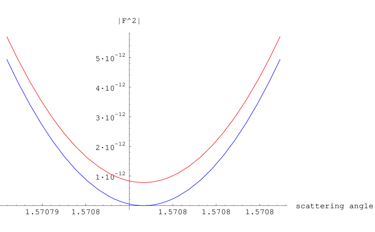
Figure 2: $|{\cal F}|^{2}$ for $t=10^{-5}$ and $x=100$.

The mod of the squares of the amplitudes are plotted for the noncommutative and the ordinary cases in Fig 2, where we see that the noncommutative amplitude does not vanish at $\Theta_{M}=\pi/2$.

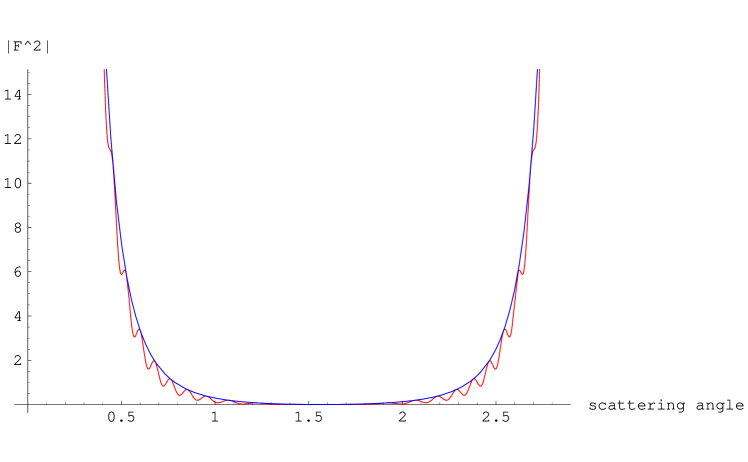
Figure 3: $|{\cal F}|^{2}$ for $t=10^{-2}$ and $x=100$.

Fig 3 shows the same process for larger values of the scattering angle. We have chosen a much larger value of $t$ to demonstrate that the noncommutative Möller scattering has characteristic modulations.

3.2 $e^{-}-e^{-}$ and Compton scattering when $\theta^{0i}=0$

In this subsection, we analyze noncommutative QED using a slightly different approach which can be efficient in the case of just space-space noncommutativity, i.e. when $\theta^{0i}=0$. In this case the only Moyal star present in Eq.(3.2) can be removed so that the interaction Hamiltonian becomes

$$H_{I}(t)=e\int d^{3}x\bar{\psi}(x)\not\!\!A(x)\psi(x)\ .$$ (3.41)

Though this looks like the interaction Hamiltonian in the commutative case, there is still the effect of noncommutativity hidden in the twisted commutation relations (3.6).

Using the map (3.9), we can map noncommutative fermionic fields to the commutative ones,

$$\psi(x) = \psi_{0}(x)e^{\frac{1}{2}\overleftarrow{\partial}_{x}\wedge{P}}\ ,$$ (3.42)

$$\overline{\psi}(x) = \overline{\psi}_{0}(x)e^{\frac{1}{2}\overleftarrow{\partial}_{x}\wedge{P}}\ ,$$

where $\psi_{0}(x)$ and $\overline{\psi}_{0}(x)$ are defined as in (3.3) for $\theta^{\mu\nu}=0$. We will need one important property which holds for any two twisted fermionic fields $a(x)=a_{0}(x)e^{\frac{1}{2}\overleftarrow{\partial}_{x}\wedge{P}}$ and $b(x)=b_{0}(x)e^{\frac{1}{2}\overleftarrow{\partial}_{x}\wedge{P}}$ (they can be $\psi$ and/or $\bar{\psi}$) which is a trivial consequence of (3.42):

$$a(x)b(x)=\big{(}(a_{0}\star b_{0})(x)\big{)}e^{\frac{1}{2}\overleftarrow{\partial}_{x}\wedge{P}}\ ,$$ (3.43)

where $\star:=*_{-\theta}$ is the “inverse Moyal star”. Using (3.43) we can write the interaction Hamiltonian as follows

$$H_{I}(t)=e\int d^{3}xA_{\mu}(x)\big{\{}\big{(}\bar{\psi}_{0}\star\gamma^{\mu}\psi_{0}(x)\big{)}e^{\frac{1}{2}\overleftarrow{\partial}_{x}\wedge{P}}\big{\}}\ .$$ (3.44)

In the same way, we have for $H_{I}(t_{x})H_{I}(t_{y})$

$$H_{I}(t_{x})H_{I}(t_{y})=$$ (3.45)

$$e^{2}\int d^{3}xd^{3}yA_{\mu}(x)A_{\nu}(y)\big{\{}\big{(}\bar{\psi}_{0}(x)\star\gamma^{\mu}\psi_{0}(x)\star_{xy}\bar{\psi}_{0}(y)\star\gamma^{\nu}\psi_{0}(y)\big{)}e^{\frac{1}{2}(\overleftarrow{\partial}_{x}+\overleftarrow{\partial}_{y})\wedge{P}}\big{\}}$$

where $\star_{xy}:=e^{-\frac{i}{2}\overleftarrow{\partial}_{x}\wedge\overrightarrow{\partial}_{y}}$ (so $\star\equiv\star_{xx}$).

Let us sketch how this approach works in the two cases of $e^{-}-e^{-}$ scattering and Compton effect.

A. $e^{-}-e^{-}$ scattering. The first observation we make is that the factor $e^{\frac{1}{2}(\overleftarrow{\partial}_{x}+\overleftarrow{\partial}_{y})\wedge{P}}$ does not contribute to the result. For the case of $e^{-}-e^{-}$ scattering the relevant term in $H_{I}(t_{x})H_{I}(t_{y})$ is hence

$$e^{2}\int d^{3}xd^{3}yA_{\mu}(x)A_{\nu}(y)\big{[}\bar{\psi}_{0}^{(+)}(x)\star\gamma^{\mu}\psi_{0}^{(-)}(x)\star_{xy}\bar{\psi}_{0}^{(+)}(y)\star\gamma^{\nu}\psi_{0}^{(-)}(y)\big{]}\ ,$$ (3.46)

where $(\pm)$ denote the positive and negative frequency modes. Using the definition of $\star$, we see that in momentum space, the overall effect of noncommutativity is the phase

$$e^{-\frac{i}{2}k_{1}\wedge k_{3}-\frac{i}{2}q_{1}\wedge q_{3}+\frac{i}{2}(k_{1}-k_{3})\wedge(q_{1}-q_{3})}\ ,$$ (3.47)

where $k_{i},q_{i}$ are integration variables.

Due to momentum conservation at every vertex, one immediately has $(k_{1}-k_{3})\wedge(q_{1}-q_{3})=0$.

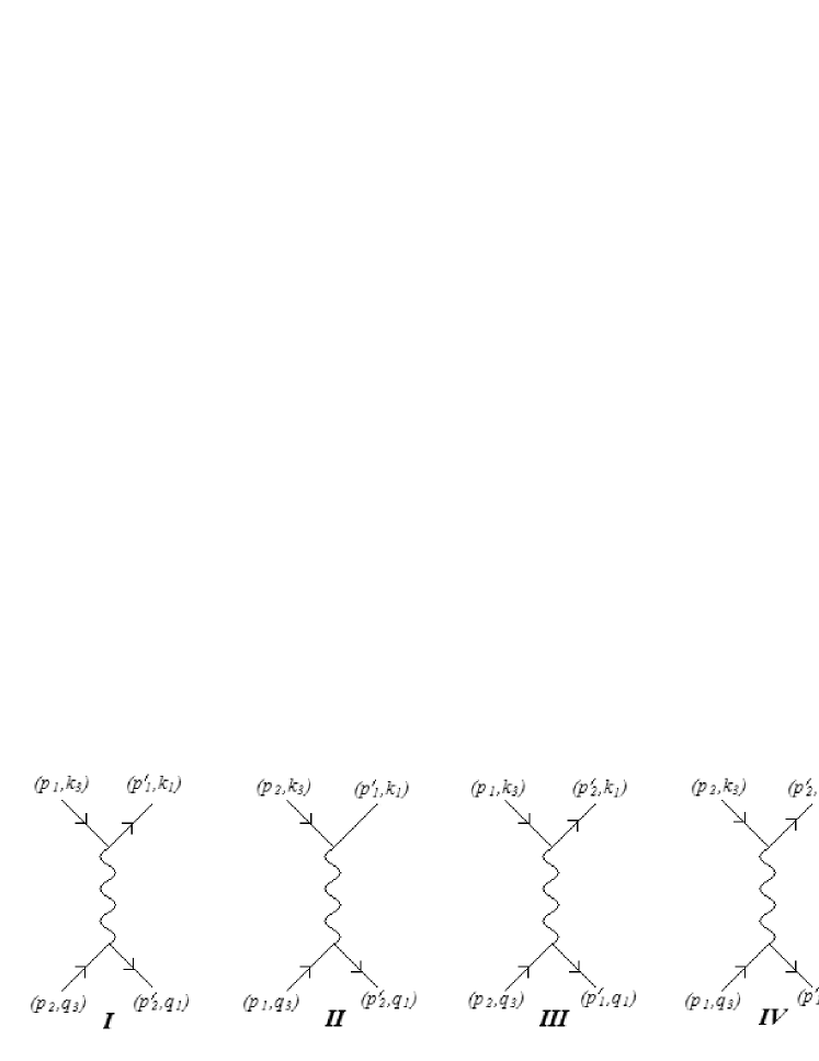
Figure 4: Feynman diagrams relevant for $e-e$ scattering.

There four different ways to assign external momenta $p_{i},p^{\prime}_{i}$. They correspond to four Feynman diagrams (see Fig 4):

$$(I) p_{1}=k_{3},\ p_{2}=q_{3},\ p^{\prime}_{1}=k_{1}\ ,p^{\prime}_{2}=q_{1}$$

$$(II) p_{2}=k_{3},\ p_{1}=q_{3},\ p^{\prime}_{1}=k_{1}\ ,p^{\prime}_{2}=q_{1}$$

$$(III) p_{1}=k_{3},\ p_{2}=q_{3},\ p^{\prime}_{2}=k_{1}\ ,p^{\prime}_{1}=q_{1}$$

$$(IV) p_{2}=k_{3},\ p_{1}=q_{3},\ p^{\prime}_{2}=k_{1}\ ,p^{\prime}_{1}=q_{1}$$

In the commutative case, diagrams (I) and (IV) are equal. The same is true for the diagrams (II) and (III). One can easily see that this is also the case in the presence of noncommutativity, but now two different diagrams have a relative phase. Including the trivial phase factor $e^{\frac{i}{2}(p_{1}\wedge p_{2}-p^{\prime}_{1}\wedge p^{\prime}_{2})}$ (this factor comes from the twisted statistics of ingoing and outgoing states), we recover the result (3.17).

B. Compton Effect. The main difference from the previous case is that we cannot get rid of the factor $e^{\frac{1}{2}(\overleftarrow{\partial}_{x}+\overleftarrow{\partial}_{y})\wedge{P}}$ in Eq.(3.45). This is due to the fact that now instead of the photon propagator, we have a spinorial one, which comes from the pairing of fields with twisted statistics. Nevertheless using the approach developed in [14], one can show that the propagator is the same as in the commutative case and enters all calculations without star products. In particular this means that all noncommutative phases will be independent of the momenta of the fields that form the propagator. Bearing this in mind, one can easily write all phases. As in the case of $e^{-}-e^{-}$ scattering, we have four different possibilities (see Fig 5):

$$(I) p_{1}=q_{3},\ p_{2}=k_{2},\ p^{\prime}_{1}=k_{1}\ ,p^{\prime}_{2}=q_{2},$$

$$(II) p_{2}=q_{2},\ p_{1}=q_{3},\ p^{\prime}_{1}=k_{1}\ ,p^{\prime}_{2}=k_{2},$$

$$(III) p_{2}=q_{2},\ p_{1}=k_{3},\ p^{\prime}_{2}=k_{2}\ ,p^{\prime}_{1}=q_{1},$$

$$(IV) p_{1}=k_{3},\ p_{2}=k_{2},\ p^{\prime}_{2}=q_{2}\ ,p^{\prime}_{1}=q_{1}.$$

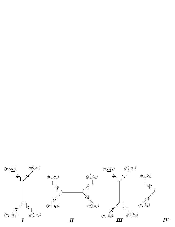
Figure 5: Feynman diagrams relevant for Compton scattering.

($k_{2},q_{2}$ are the photon momenta. This is why they were absent for the $e^{-}-e^{-}$ scattering.) In the commutative case, diagrams (I) and (III) are equal. The same is true for the diagrams (II) and (IV). Here the similarities with the case of $e^{-}-e^{-}$ scattering end. Whereas in that case before the integration over $k_{i},q_{i}$ the phases were equal to Eq.(3.47) for all four diagrams, here the situation is different:

$$\mbox{Phases for }(I)\mbox{ and }(II): e^{-\frac{i}{2}k_{1}\wedge q_{3}}e^{\frac{i}{2}(k_{1}-q_{3})\wedge p_{1}}$$

$$\mbox{Phases for }(III)\mbox{ and }(IV): e^{-\frac{i}{2}k_{3}\wedge q_{1}}e^{\frac{i}{2}(-k_{3}+q_{1})\wedge p_{1}}$$

The second factor in both cases comes when $e^{\frac{1}{2}(\overleftarrow{\partial}_{x}+\overleftarrow{\partial}_{y})\wedge{P}}$ picks up the momentum $p_{1}$ of the incoming electron. As a result, in the case of Compton scattering, the effect of the interference between two commutative diagrams is not present. One rather has that the commutative amplitude $\mathcal{T}_{com}$ gets multiplied by the overall $\theta$-dependent factor:

$$\mathcal{T}_{nc}=\frac{1+e^{-ip_{1}\wedge p^{\prime}_{1}}}{2}\mathcal{T}_{com}\ .$$ (3.48)

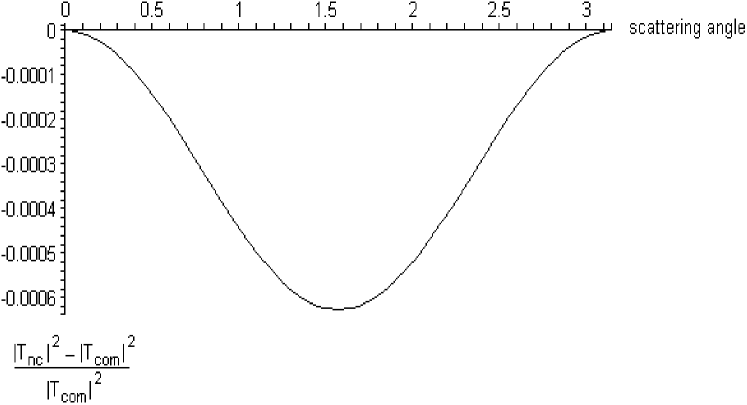
Figure 6: $\frac{|\mathcal{T}_{nc}|^{2}-|\mathcal{T}_{com}|^{2}}{|\mathcal{T}_{com}|^{2}}$ as a function of the scattering angle for Compton scattering, for $t=10^{-5}$ and $x=100$

Fig. 6 plots the relative deviation of the scattering cross-section between the noncommutative and commutative cases for Compton scattering.

4 Causality and Lorentz Invariance

For the purposes of our discussion, causality will have the meaning it takes in standard local quantum field theories. Thus if $\rho(\xi)$ is an observable local field $\rho$ like the electric charge density localized at a spacetime point $\xi$, and $x$ and $y$ are spacelike separated points ($x\sim y$), then (local) causality states that

$$[\rho(x),\rho(y)]=0.$$ (4.1)

It means that they are simultaneously measurable.

Causal set theory (see for example [15] for a recent review) uses a sense of causality which differs from (4.1). There is also a criticism of the conceptual foundations of (4.1) by Sorkin [16].

Let $H_{I}$ be the interaction Hamiltonian density in the interaction representation. The interaction representation $S$-matrix is

$$S=T\exp\left(-i\int d^{4}xH_{I}(x)\right).$$ (4.2)

Bogoliubov and Shirkov [8] long ago deduced from causality and relativistic invariance that $H_{I}$ is a local field:

$$[H_{I}(x),H_{I}(y)]=0,x\sim y$$ (4.3)

Later Weinberg discussed [9, 10] discussed the fundamental significance of (4.3): if (4.3) fails, $S$ is not relativistically invariant. He argued as follows.

Let us assume the conventional transformation law for $H_{I}$ under Lorentz transformation $\Lambda$:

$$H_{I}(x)\rightarrow H_{I}(\Lambda^{-1}x).$$ (4.4)

Then we can argue that $S$ is Lorentz invariant provided time-ordering $T$ does not spoil it.

We can see this as follows. In the absence of time-ordering $T$, the second order term in $H_{I}$ in (4.2) is

$$\frac{(-i)^{2}}{2!}\int d^{4}xd^{4}yH_{I}(x)H_{I}(y)=-\frac{1}{2}\tilde{H}_{I}(0)\tilde{H}_{I}(0)$$ (4.5)

where $\tilde{H}_{I}(0)$ is the zero four-momentum component of $H_{I}(x)$:

$$\tilde{H}_{I}(p)=\int\frac{d^{4}x}{(2\pi)^{4}}e^{ip\cdot x}H_{I}(x)$$ (4.6)

We must transform (4.5) according to (2.16). As zero four-momentum states are both translation- and Lorentz-invariant, we see that (4.5) is Lorentz invariant under the twisted coproduct. This argument extends to all orders in $H_{I}$ (assuming that long-range (infrared) effects do not spoil it).

Consider next the second order term $S^{(2)}$ in $S$. It is the leading term influenced by time-ordering:

$$S^{(2)}=\frac{(-i)^{2}}{2!}\int d^{4}xd^{4}yT(H_{I}(x)H_{I}(y)).$$ (4.7)

Now

$$T(H_{I}(x)H_{I}(y)) = \theta(x_{0}-y_{0})H_{I}(x)H_{I}(y)+x\leftrightarrow y$$ (4.8)

$$= H_{I}(x)H_{I}(y)-\theta(y_{0}-x_{0})[H_{I}(x),H_{I}(y)]\,.$$ (4.9)

Under a Lorentz transformation $\Lambda$,

$$U(\Lambda)T(H_{I}(x)H_{I}(y))U(\Lambda)^{-1}=H_{I}(\Lambda^{-1}x)H_{I}(\Lambda^{-1}y)-\theta(y_{0}-x_{0})[H_{I}(\Lambda^{-1}x),H_{I}(\Lambda^{-1}y)].$$ (4.10)

We exclude the anti-unitary time-reversal from our discussion. Then we see that $S$ is Lorentz-invariant if

$$\theta(y_{0}-x_{0})[H_{I}(\Lambda^{-1}x),H_{I}(\Lambda^{-1}y)]=\theta[\Lambda^{-1}(y-x)_{0}][H_{I}(\Lambda^{-1}x),H_{I}(\Lambda^{-1}y)].$$ (4.11)

For time- (and light-) like separated $x$ and $y$, $\theta(y_{0}-x_{0})$ is Lorentz-invariant:

$$\theta(y_{0}-x_{0})=\theta(\Lambda^{-1}(y-x)_{0}),\quad x\not\sim y\,,$$ (4.12)

and in that case, (4.11) is fulfilled. But if $x\sim y$, time ordering can be reversed by a suitable Lorentz transformation. Hence Lorentz invariance of $S$ suggests locality:

$$[H_{I}(x),H_{I}(y)]=0\quad x\sim y\,.$$ (4.13)

[A generalized form of (4.13) may be enough. See [11].] Incidentally, we cannot say that (4.3) [together with (4.4)] is enough for Lorentz invariance. $H_{I}$ may fulfill (4.3), but $[H_{I}(x),H_{I}(y)]$ may contain derivative terms, such as happens in a charged massive vector meson theory, which spoil Lorentz invariance [9].

The interaction density in the electron-photon system for $\theta^{\mu\nu}\neq 0$ is

$$H_{I}(x)=ie(\bar{\psi}*\gamma^{\rho}A_{\rho}\psi)(x)\,.$$ (4.14)

For simplicity we consider the case where

$$\theta^{0i}=0,\quad\theta^{ij}\neq 0$$ (4.15)

and show that (4.3) is violated. Hence $S$ is not Lorentz-invariant. It can be checked that (4.13) is violated if $\theta^{0i}\neq 0$ even if $\theta^{ij}=0$. We can also directly see from the explicit formula for $e^{-}-e^{-}$ scattering amplitude in Section 8 that it is not Lorentz-invariant if $\theta^{\mu\nu}\neq 0$.

With (4.15),

$$S=T\exp\left(-i\int d^{3}xH_{I}(x)\right)=T\exp\left(-i\int\hat{H}_{I}(x)\right),\quad\hat{H}_{I}(x)=ie(\bar{\psi}\gamma^{\rho}A_{\rho}\psi)(x)$$ (4.16)

We have used the property of the Moyal product to remove the $*$ from $H_{I}$. That is possible although $H_{I}$ is integrated only over spatial variables because of (4.15). But there is still the effect of $\theta^{\mu\nu}$ in the oscillator modes of $\psi$ and $\bar{\psi}$. Let $\psi_{0}$ be the limit of $\psi$ for $\theta^{\mu\nu}=0$ and $P_{\mu}$ be the momentum operator for $\psi$ (which is the same as for $\psi_{0}$). Then using (3.9),

$$\hat{H}_{I}(x) = J^{\lambda}(x)A_{\lambda}(x)$$ (4.17)

$$J^{\lambda}(x) = J^{(0)\lambda}(x)e^{\frac{1}{2}\overleftarrow{\partial}_{\mu}\theta^{\mu\nu}P_{\nu}}\,,$$ (4.18)

$$J^{(0)\lambda}(x) = ie\bar{\psi}_{0}\gamma^{\lambda}\psi_{0}.$$ (4.19)

As $A_{\lambda}$ is not affected by twisting, $[A_{\lambda}(x),A_{\rho}(y)]$ is zero for $x\sim y$. The entire effect of $\theta^{\mu\nu}$ is in $J^{\lambda}$. But

$$J^{\lambda}(x)J^{\rho}(y)\neq J^{\rho}(y)J^{\lambda}(x),x\sim y,$$ (4.20)

because of the exponential following $J^{(0)\lambda}$. One can check (4.20) by retaining just a pair of distinct momentum modes in $J^{\lambda}(x)$ and another such pair in $J^{\rho}(y)$.

Thus $S$ is not Lorentz invariant.

Acknowledgments: It is a pleasure to thank T. R. Govindarajan for suggesting that we look for zeroes of $e^{-}-e^{-}$ scattering. The work of APB, AP and BQ is supported in part by DOE under grant number DE-FG02-85ER40231.

References

• [1] M. Chaichian, P. P. Kulish, K. Nishijima and A. Tureanu, Phys. Lett.B 604, 98 (2004); [arXiv:hep-th/0408069].
• [2] J. Wess, arXiv:hep-th/0408080.
• [3] A.P. Balachandran, G. Mangano, A. Pinzul, S. Vaidya, Int. J. Mod. Phys. A 21, 3111 (2006); [arXiv:hep-th/0508002].
• [4] A. P. Balachandran, A. Pinzul and B. Qureshi, Phys. Lett. B 634, 434 (2006); [arXiv:hep-th/0508151].
• [5] A. P. Balachandran, A. Pinzul, B. A. Qureshi and S. Vaidya, Phys. Rev.  D 76, 105025 (2007) [arXiv:0708.0069 [hep-th]].
• [6] A. P. Balachandran and B. A. Qureshi, arXiv:0903.0478 [hep-th].
• [7] D. Bahns, S. Doplicher, K. Fredenhagen and G. Piacitelli, Phys. Lett. B 533, 178 (2002) [arXiv:hep-th/0201222].
• [8] N. N. Bogoliubov and D. V. Shirkov, “Introduction to the Theory of Quantized Fields” Interscience Publishers, New York, 1959.
• [9] S. Weinberg, Phys. Rev.  133, B1318 (1964).
• [10] S. Weinberg, “The Quantum theory of fields. Vol. 1: Foundations,” Cambridge University Press, Cambridge, 1995.
• [11] A. P. Balachandran, A. Pinzul, B. A. Qureshi and S. Vaidya, Phys. Rev.  D 77, 025020 (2008); [arXiv:0708.1379 [hep-th]].
• [12] X. Calmet, Phys. Rev. D 71, 085012 (2005) [arXiv:hep-th/0411147].
• [13] X. Calmet and A. Kobakhidze, Phys. Rev. D 72, 045010 (2005) [arXiv:hep-th/0506157].
• [14] A. Pinzul, Int. J. Mod. Phys. A 20, 6268 (2005).
• [15] F. Dowker, “Causal sets and the deep structure of spacetime”, [arXiv:gr-qc/0508109].
• [16] R. D. Sorkin, [arXiv:gr-qc/9302018].