Stabilization of the Extra Dimensions in Brane Gas Cosmology with Bulk Flux

Abstract

We consider the anisotropic evolution of spatial dimensions and the stabilization of internal dimensions in the framework of brane gas cosmology. We observe that the bulk RR field can give an effective potential which prevents the internal subvolume from collapsing. For a combination of $(D-3)$-brane gas wrapping the extra dimensions and 4-form RR flux in the unwrapped dimensions, it is possible that the wrapped subvolume has an oscillating solution around the minimum of the effective potential while the unwrapped subvolume expands monotonically. The flux gives a logarithmic bounce to the effective potential of the internal dimensions.

I Introduction

There has been considerable effort during the past decade in the area of higher dimensional gravity where the four-dimensional gravity can be recovered as an effective theory. In the theory of general relativity, the dimensionality of the universe is an assumption. It is not derived dynamically from a fundamental theory. However, unifying gravity with other forces of nature strongly suggests that there may be more than three spatial dimensions. One plausible explanation can be given by string theory, which is higher dimensional. A mechanism to generate three spatial dimensions was proposed in Refs. bv and tv . This is a mechanism to generate dynamically the spatial dimensionality of spacetime and to explain the problem of initial singularity. The key ingredient of this model is based on the symmetry of string theory, called T-duality. With this symmetry, spacetime has a topology of a nine-dimensional torus, and its dynamics is driven by a gas of fundamental strings. Since strings have (1+1)-dimensional world volumes, they can intersect in 2(1+1) spacetime dimensions or less from the topological point of view. The winding modes can annihilate the anti-winding modes if they meet. Once the windings are removed from the dimensions, these dimensions can expand into the large directions that we observe today. Thus, with a gas of strings, three spatial dimensions can become large.

With the realization of D-branes in string theory polch , there had been attempts to study string cosmology with a gas of D-branes including strings magrio ; psl . The mechanism of Brandenberger and Vafa (BV) in Refs. bv ; tv was reconsidered in this new framework of string theory. Authors of Ref. abe argued that when branes are included, strings still dominate the evolution of the universe at late times. This model of brane gas cosmology was studied extensively bgextended ; cbbc ; kayarador ; egjk1 ; jykim ; modulstab ; campos ; Cheungwatsonbran (see also bW0510022 for comprehensive reviews). In the picture of brane gas cosmology, the universe starts from a hot, dense gas of D-branes in thermal equilibrium. The winding modes of branes prevent the spatial dimensions from growing. Branes with opposite winding numbers can annihilate if their world volumes intersect. Thus, a hierarchy of scales can be achieved between wrapped and unwrapped dimensions. Though the BV mechanism can trigger the onset of cosmological evolution based on string theory, this does not guarantee the answer to the question why there are three large spatial dimensions while others remain small. There have been attempts to yield the anisotropic expansion based on certain wrappings of the brane gases egjk1 ; jykim .

It is well known that the stability of internal dimensions cannot be achieved with string or brane gases of purely winding modes. Stabilizing the extra dimensions is an important issue in string or brane gas cosmology modulstab ; campos ; Cheungwatsonbran ; patil1 ; patil2 . For a particular configuration of brane gas in eleven dimensional supergravity, Campos campos has shown the importance of fluxes in stabilizing the internal dimensions through numerical computations of the evolution equations for wrapped and unwrapped dimensions. It is shown that all internal dimensions, except the dilaton, are dynamically stabilized in the presence of two-form flux with a gas of long strings Cheungwatsonbran . In certain string theories patil2 , special string states can stabilize the extra dimensions for fixed dilaton. Massless string modes at self-dual radius play a crucial role for the radion stabilization.

In this work we will focus on the anisotropic evolution of spatial dimensions and the stabilization of internal dimensions based on a certain configuration of branes and bulk background field. We consider the possible stabilization of internal dimensions with bulk Ramond-Ramond (RR) field. We observe that the bulk RR field can give an effective potential which prevents the internal volume from collapsing. The flux gives a logarithmic bounce to the effective potential of the internal volume.

In Sec. II, we consider the brane universe in the frame of Einstein gravity. We present a formalism for anisotropic expansion of brane universe and show that it is impossible to stabilize the internal volume with brane gases only. In Sec. III, we set up a supergravity formalism with brane gas and bulk RR field. For the anisotropic expansion, we consider the global rotational symmetry is broken down to $SO(p)\times SO(D-p)$ by $(D-p)$-brane gas. We decouple the equations of motion for each subvolumes of $SO(p)$ and $SO(D-p)$ and argue the possible stabilization. In Sec. IV, we conclude and discuss.

II Anisotropic expansion of brane universe

In the previous work of us jykim , we have shown that the extra dimensions should be wrapped with three- or higher-dimensional branes for the observed three large spatial dimensions. However, it is not guaranteed that the compact dimensions can be stabilized with these branes. We start, after the thermal equilibrium of brane gas is broken, from the case when three dimensions are unwrapped and $D-3$ dimensions are wrapped by gas of branes whose dimensions are less than or equal to $D-3$. We assume that each type of brane gases makes a comparable contribution to the energy momentum density. Then, we can study the evolution of a universe based on the following form of metric

$$g_{MN}={\rm diag}(-1,a^{2}\delta_{ij},b^{2}\delta_{mn}),$$ (1)

where $a^{2}$ is the scale factor of the $3$-dimensional space and $b$ is the scale factor of the internal $(D-3)$-dimensional subspace.

The evolution of the universe with the above setting is equivalent to the asymmetric inflation in the brane world scenario adkmr . We will consider a universe which can be described by the effective action

$$S=\int d^{D+1}x\sqrt{g}\Big{[}\frac{R}{2\kappa^{2}}-V_{D+1}(g_{\mu\nu})\Big{]},$$ (2)

where $\kappa^{2}=1/M^{D-1}_{*}$, $M_{*}$ being the $(D+1)$-dimensional unification scale, and $V_{D+1}(g_{\mu\nu})$ is the effective potential for the metric generated by the breakdown of the Poincare invariance. Considering the spatial section to be a $D$-dimensional torus $T^{D}$, we write the metric as

$$ds^{2}=-n^{2}dt^{2}+\sum_{k}a^{2}_{k}(t)(dx_{k})^{2}.$$ (3)

Technically, we retain the lapse $n$ because we work on the action to reduce the action to a one-dimensional effective action. When we vary the reduced action with respect to the lapse, we obtain the Hamiltonian constraint. Later, we will set $n=1$. Also we use the metric (3) instead of metric (1) to produce the correct combinational factors when the partial derivatives are taken over different scale factors. After all the derivatives are evaluated, we will take the identities $a_{1}=\cdots=a_{3}=a$ and $a_{4}=\cdots=a_{D}=b$.

The effective potential $V_{D+1}$ arising from the brane tensions can be written as

$$\sqrt{g}V_{D+1}(g_{\mu\nu})=n\Big{[}\Lambda_{D}\prod_{k=1}^{D}a_{k}+\sum_{\{p\}}T_{\{p\}}\prod_{\{p\}}a_{k}+\prod_{k=1}^{D}a_{k}U(a_{k})\Big{]},$$ (4)

where $\Lambda_{D}$ is the tension of a $D$-dimensional space-filling brane which can be considered as a bulk cosmological constant, $T_{\{p\}}$ is the tension of $p$-brane averaged over space, and $U(a_{k})$ parameterizes all contributions to the potential other than branes. For example, Fluxes, curvatures, and brane-brane interactions can give non-zero terms to $U(a_{k})$. We will show that $U(a_{k})$ plays an important role for the internal dimensions from collapsing to zero. In the summation over the brane tension, the notation $\{p\}$ refers to the fact that there may be branes with the same $p$ oriented along different directions. For example, 2-brane can wrap (12) cycle, (23) cycle et cetera.

Now, we evaluate the Ricci scalar in Eq. (3) and reduce the problem to the motion of a particle in $D$ dimensions. The one-dimensional effective action for the scale factors $a_{k}$ is

$$S_{\rm eff} =-{\cal V}_{D}\int dt~{}n\prod_{k=1}^{D}a_{k}\Big{[}\frac{1}{2\kappa^{2}}\Big{\{}(\sum_{j=1}^{D}\frac{\dot{a}_{j}}{na_{j}})^{2}-\sum^{D}_{j=1}(\frac{\dot{a}_{j}}{na_{j}})^{2}\Big{\}}$$ (5)

$$~{}~{}~{}~{}~{}~{}~{}~{}~{}~{}~{}~{}~{}~{}~{}~{}~{}~{}~{}~{}~{}~{}~{}~{}~{}~{}+\Lambda_{D}+\frac{1}{\prod_{n=1}^{D}a_{n}}\sum_{\{p\}}T_{\{p\}}{\prod_{\{p\}}a_{k}}+U(a_{k})\Big{]},$$

where ${\cal V}_{D}=\int d^{D}x$ is the coordinate spatial volume, which contains the branes, and is dimensionless. In these units, the scale factors $a_{k}$ are dimension-full quantities, with dimension $M^{-1}_{*}$. If we vary this action with respect to $n$ and $a_{k}$, we obtain the following set of equations of motion after some straightforward algebra and setting $n=1$ at the end,

$$(\sum_{j=1}^{D}\frac{\dot{a}_{j}}{a_{j}})^{2}-\sum_{j=1}^{D}(\frac{\dot{a}_{j}}{a_{j}})^{2}=2\kappa^{2}\{\Lambda_{D}+U(a_{k})\}+\frac{2\kappa^{2}}{\prod_{k=1}^{D}a_{k}}\sum_{\{p\}}T_{\{p\}}\prod_{\{p\}}a_{k},$$ (6)

$$\frac{\ddot{a}_{n}}{a_{n}}+\sum_{l\neq n}\frac{\dot{a}_{n}\dot{a}_{l}}{a_{n}a_{l}} = \frac{2\kappa^{2}}{D-1}\{\Lambda_{D}+U(a_{k})\}+\frac{\kappa^{2}}{(D-1)\prod_{k=1}^{D}a_{k}}\sum_{\{p\}}T_{\{p\}}\prod_{\{p\}}a_{k}$$ (7)

$$+ \frac{\kappa^{2}}{(D-1)\prod_{k=1}^{D}a_{k}}\sum_{l=1}^{D}\sum_{\{p\}}T_{\{p\}}a_{l}\frac{\partial}{\partial a_{l}}\prod_{\{p\}}a_{k}$$

$$- \frac{\kappa^{2}}{\prod_{k=1}^{D}a_{k}}\sum_{\{p\}}T_{\{p\}}a_{n}\frac{\partial}{\partial a_{n}}\prod_{\{p\}}a_{k}-\kappa^{2}a_{n}\frac{\partial U}{\partial a_{n}}+\frac{\kappa^{2}}{D-1}\sum_{k=1}^{D}a_{k}\frac{\partial U}{\partial a_{k}}.$$

We emphasize here that the partial derivatives are meant to be taken over different scale factors, even if some of the scale factors may coincide on the background. Note that the derivative operator $a_{l}\frac{\partial}{\partial a_{l}}$ behaves like a counting operator acting on $\prod_{\{p\}}a_{k}$. If $\prod_{\{p\}}a_{k}$ depends on $a_{l}$, the operator produces $1$; otherwise, it gives $0$. Hence, the operator $\sum_{l}a_{l}\frac{\partial}{\partial a_{l}}$ simply counts the dimension of the brane.

Now, we consider the special case when the global rotational symmetry is broken down to $SO(3)\times SO(D-3)$ by effective $(D-3)$-branes whose tension we denote $T_{D-3}$. We ignore the stabilizing potential $U(a_{k})$ for simplicity. In this case, the equations of motion in Eqs. (6) and (7) are simplified to, taking units in which $2\kappa^{2}=1$,

$$6(\frac{\dot{a}}{a})^{2}+(D-3)(D-4)(\frac{\dot{b}}{b})^{2}+6(D-3)\frac{\dot{a}\dot{b}}{ab}=\Lambda_{D}+\frac{T_{D-3}}{a^{3}},$$ (8)

$$\frac{\ddot{a}}{a}+2(\frac{\dot{a}}{a})^{2}+(D-3)\frac{\dot{a}\dot{b}}{ab}=\frac{\Lambda_{D}}{D-1}+\frac{D-2}{2(D-1)}\frac{T_{D-3}}{a^{3}},$$ (9)

$$\frac{\ddot{b}}{b}+(D-4)(\frac{\dot{b}}{b})^{2}+3\frac{\dot{a}\dot{b}}{ab}=\frac{\Lambda_{D}}{D-1}-\frac{1}{2(D-1)}\frac{T_{D-3}}{a^{3}}.$$ (10)

The largest difference between the sizes $a$ and $b$ can be induced if $a$ grows faster than $b$, as dictated by Eqs. (9) and (10). The key parameters for controlling the relative rates of growth of $a$ and $b$ are their accelerations, not their velocities. To ensure that $a$ exceeds $b$ by many orders of magnitude, the sources in Eqs. (9) and (10) must produce the slow-roll conditions for $b$, making its acceleration small or negative while keeping the acceleration of $a$ positive.

If the volumes of wrapped and unwrapped subspaces are defined as

$$\zeta\equiv a^{3},~{}~{}~{}~{}\xi\equiv b^{D-3},$$ (11)

the second derivative terms in Eqs. (9) and (10) can be written as

$$\frac{\ddot{\zeta}}{\zeta}+\frac{\dot{\zeta}\dot{\xi}}{\zeta\xi} = 3\Big{\{}\frac{\Lambda_{D}}{D-1}+\frac{D-2}{2(D-1)}\frac{T_{D-3}}{\zeta}\Big{\}},$$ (12)

$$\frac{\ddot{\xi}}{\xi}+\frac{\dot{\zeta}\dot{\xi}}{\zeta\xi} = (D-3)\Big{\{}\frac{\Lambda_{D}}{D-1}-\frac{1}{2(D-1)}\frac{T_{D-3}}{\zeta}\Big{\}}.$$ (13)

The above equations of motion reduce to a simple form by removing the coupled first-derivative terms:

$$\frac{\ddot{\xi}}{\xi}-\frac{D-6}{D-1}\Lambda_{D}=\frac{\ddot{\zeta}}{\zeta}-\frac{4D-9}{2(D-1)}\frac{T_{D-3}}{\zeta}.$$ (14)

Since the left-hand side of Eq. (14) is a function of $\xi$ while the right-hand side is a function of $\zeta$, each side should be the same constant. Taking the constant as the parameter $E$, we have the following set of decoupled equations for $\zeta$ and $\xi$:

$$\frac{\ddot{\zeta}}{\zeta} = E+\frac{4D-9}{2(D-1)}\frac{T_{D-3}}{\zeta},$$ (15)

$$\frac{\ddot{\xi}}{\xi} = E+\frac{D-6}{D-1}\Lambda_{D}.$$ (16)

Note that the constant $E$ is not an independent parameter. For the given configuration of branes, it is related to brane tension $T_{D-3}$ and cosmological constant $\Lambda_{D}$. The constant $E$ can be found by putting the solutions of (15) and (16) into the original equation (12) and (13).

To make the unwrapped subvolume $\zeta$ expand forever, we require the constant $E$ to be a positive definite. Then, the solution for the subspace $\zeta$ is

$$\zeta=(\zeta_{0}+C_{1})e^{\gamma t}-C_{1},$$ (17)

where $\zeta_{0}$ is the volume of unwrapped subspace at $t=0$, $\gamma=\sqrt{E}$, and $C_{1}=\frac{4D-9}{2(D-1)}\frac{T_{D-3}}{E}$. For given $E$, three types of solution for $\xi$ are possible depending on the bulk cosmological constant $\Lambda_{D}$. First, for $\Lambda_{D}>0$, we have

$$\xi=\xi_{0}e^{\gamma_{1}t},~{}~{}\gamma_{1}=\sqrt{E+\frac{D-6}{D-1}\Lambda_{D}}.$$ (18)

Since $\gamma_{1}>\gamma$, $\xi$ expands faster than $\zeta$. This means that the wrapped dimensions expand faster than the unwrapped dimensions. To determine the constant $E$, we put the solutions (17) and (18) into (12)

$$\gamma^{2}(1+\frac{C_{1}}{\zeta})+\gamma\gamma_{1}(1+\frac{C_{1}}{\zeta})=3\Big{\{}\frac{\Lambda_{D}}{D-1}+\frac{D-2}{2(D-1)}\frac{T_{D-3}}{\zeta}\Big{\}}.$$ (19)

This gives the following relation between the constant $E$ and other parameters in the unit of $2\kappa^{2}=1$,

$$\gamma^{2}+\gamma\gamma_{1} = 3\frac{\Lambda_{D}}{D-1},$$ (20)

$$(\gamma^{2}+\gamma\gamma_{1})C_{1} = \frac{3(D-2)}{2(D-1)}T_{D-3}.$$ (21)

There is no positive value of $E$ which can suffice both of the above equations. This means that the solutions of the types (17) and (18) are not possible.

Second, for $\Lambda_{D}=-|\Lambda_{D}|<0$ and $E-\frac{D-6}{D-1}|\Lambda_{D}|>0$, the possible solution for $\xi$ is of the form

$$\xi=\xi_{0}e^{\gamma_{2}t},~{}~{}\gamma_{2}=\sqrt{E-\frac{D-6}{D-1}|\Lambda_{D}|}.$$ (22)

In this case, $\xi$ expands slower than $\zeta$. Repeating the same procedure as in the previous case, to check whether this solution can be realized, we have

$$\gamma^{2}+\gamma\gamma_{2} = -3\frac{|\Lambda_{D}|}{D-1},$$ (23)

$$(\gamma^{2}+\gamma\gamma_{2})C_{1} = \frac{3(D-2)}{2(D-1)}T_{D-3}.$$ (24)

Since $E>0$ is a strict condition for the expansion of the unwrapped dimensions, it is obvious that the first condition cannot be satisfied.

Finally, for $\Lambda_{D}=-|\Lambda_{D}|<0$ and $E-\frac{D-6}{D-1}|\Lambda_{D}|<0$, we have

$$\xi=\xi_{0}\cos(\omega t),~{}~{}\omega=\sqrt{-E+\frac{D-6}{D-1}|\Lambda_{D}|}.$$ (25)

In this case, the wrapped internal subvolume $\xi$ oscillates while the unwrapped volume $\zeta$ expands monotonically. The solution seems quite similar to the one found by Patil and Brandenberger patil1 in string gas cosmology in five dimensional spacetime without dilaton. They found that an oscillating type of solution, where the radius of extra dimension oscillates at the self-dual radius, is one of the possible trajectories. To check whether there is any constant $E$ which gives this possibility, we substitute (17) and (25) into (12)

$$\gamma^{2}(1+\frac{C_{1}}{\zeta})+\omega\gamma(1+\frac{C_{1}}{\zeta})\tan\omega t=3\Big{\{}\frac{-|\Lambda_{D}|}{D-1}+\frac{D-2}{2(D-1)}\frac{T_{D-3}}{\zeta}\Big{\}}.$$ (26)

It obvious that there is no nontrivial solution. We conclude, from the results for the three cases, that it is not possible to stabilize the internal dimensions with only branes.

The above analysis with effective $(D-3)$-branes is a special case of the dynamics described by Eq. (7). Other distributions of brane sources can give different possibilities. However, to have three large observed dimensions, we cannot neglect the potential $U(a_{k})$ which represents the potential other than branes. Considering the motion of two subvolumes $\zeta$ and $\xi$ as motion of particles in one-dimension effective potentials, the crucial point is that there is no bouncing potential for small $\xi$ for the third case in which we are interested. So the size of the internal subvolume is not bounded from below. This means that the internal subvolume can shrink to zero and can have even negative value, violating the assumption of the late-time brane gas approximation.

III Brane gas cosmology with bulk RR field

Having established the formalism and shown that it is not possible to stabilize the internal volume with only brane gas, let us consider a model where the potential $U(a_{k})$ comes from bulk flux. The model we will consider is type II string theory compactified on $T^{9}$. Also we consider the late stage of the BV scenario where the radii and curvature scales are grown larger than the ten-dimensional Planck length. Since winding numbers are topologically conserved, only branes with opposite orientations can cause unwinding. This unwinding interactions are very short ranged since this happens when the world volumes of branes and antibranes physically intersect as in BV scenario bv . When the radii of the unwound directions have grown enough, the brane and antibrane densities will be diluted so that they cannot find each other to intersect. Then we can neglect the brane-antibrane annihilation since this term will be turned off as the transverse dimensions expand kayarador ; egjk1 ; jykim . Supergravity is a good approximation with the growing radii and falling temperature. In brane gas cosmology it is assumed that brane mode fluctuations are small and only winding modes dominate the cosmological evolution. So we consider the wrapped D-branes, which do not interact with each other, for the matter part of the Einstein equation. This corresponds to a classical approximation of the brane dynamics. Assuming that the brane gases are homogeneous, we can take the average of the contributions of all kinds of branes to the energy-momentum tensor.

In the point of string theory, the gravitational interaction is described by the coupled system of the metric and dilaton. Dilaton plays an important role in the large-small symmetry of string theory called T-duality. The initial big-bang singularity can be resolved in terms of T-duality bv ; tv . We start from the following bulk effective action of type II string theory

$$S_{\rm b}=\frac{1}{2\kappa^{2}}\int d^{D+1}x\sqrt{-g}\Bigl{[}e^{-2\phi}\{R+4(\nabla\phi)^{2}\}-\frac{1}{2l!}F_{l}^{2}-V(\phi)\Bigr{]},$$ (27)

where $\phi$ is the dilaton field, $F_{l}$ is an RR $(l)$-form field strength and $V(\phi)$ is the dilaton potential. The dilaton potential is a product of nonperturbative effects. For simplicity, we consider only flat potential which equivalently is a cosmological constant.

The matter contribution of a single brane to the action is represented by the Dirac-Born-Infeld (DBI) action of $p$-brane

$$S_{\rm p}=-T_{p}\int d^{p+1}\xi e^{-\phi}\sqrt{-{\rm det}({\hat{g}}_{\mu\nu}+{\hat{B}}_{\mu\nu}+2\pi\alpha^{\prime}{F}_{\mu\nu})},$$ (28)

where ${\hat{g}}_{\mu\nu}$ is the induced metric to the brane

$${\hat{g}}_{\mu\nu}=g_{MN}\frac{\partial x^{M}}{\partial\xi^{\mu}}\frac{\partial x^{N}}{\partial\xi^{\nu}}.$$ (29)

Here $M,N$ are the indices of bulk spacetime and $\mu,\nu$ are those of brane. ${\hat{B}}_{\mu\nu}$ is the induced antisymmetric tensor field and ${F}_{\mu\nu}$ is the field strength tensor of gauge fields $A_{\mu}$ living on the brane. The fluctuations of the brane coordinates and other fields within the brane are negligible when the temperatures are low enough. So we neglect ${\hat{B}}_{\mu\nu}$ and ${F}_{\mu\nu}$ terms below. The total action can be written as

$$S_{\rm tot}=S_{\rm b}+\sum_{\{p\}}S_{\{\rm p\}}.$$ (30)

Since we are interested in the late time cosmology, we have to work in the Einstein frame defined by $g_{MN}^{\rm S}=e^{\frac{4}{D-1}\phi}g_{MN}^{\rm E}$. The formalism and physical picture for the investigation of metric perturbations have been developed in the Einstein frame where one can use the standard simple Einstein equations. Since the weak coupling limit (i.e. $g_{s}=e^{\phi}<<1$) is one of the basic assumptions of string/brane gas cosmology, we ignore the running of dilaton assuming that dilaton can be stabilized. When the dilaton is not running, the two frames are equivalent since the contribution of constant dilaton can be absorbed in the redefinition of brane tension and RR field. Then, the action can be written as

$$S_{\rm b}^{E}=\frac{1}{2\kappa^{2}}\int d^{D+1}x\sqrt{-g^{E}}\Bigl{[}R-\frac{1}{2l!}F_{l}^{2}-\Lambda_{D}\Bigr{]},$$ (31)

$$S_{\rm p}=-T_{p}\int d^{p+1}\xi\sqrt{-{\rm det}{\hat{g}}_{\mu\nu}^{E}}.$$ (32)

We drop the superscript $E$ from now on.

In the point of bulk theory, the energy momentum tensor of a single D$p$-brane has a delta function singularity at the position of the brane along the transverse directions

$$\sqrt{-g}T_{p}^{MN}=-T_{p}\int d^{p+1}\xi\sqrt{-{\hat{g}}}{\hat{g}}^{\mu\nu}\partial_{\mu}x^{M}\partial_{\nu}x^{N}\delta[x-x(\xi)].$$ (33)

In cosmological setting, it seems natural to take a gas of such branes in a continuum approximation and this smooths the singularity by integrating over the transverse dimensions kayarador .

The induced metric on the $p$-brane follows from its embedding in the bulk. We choose the static gauge $\xi^{\mu}=x^{\mu}$ ($\mu=0,1,\dots,p$) and suppose the simple embedding $x^{i}=x^{i}(t)$ for $i=p+1,\dots,D$. The induced metric on the brane is,

$${\hat{g}}_{\mu\nu}={\rm diag}\{-(1-v^{2}),a_{1}^{2},a_{2}^{2},\dots,a_{p}^{2}\},$$ (34)

where $v^{2}=\sum_{i=p+1}^{D}{\dot{x}}^{i}{\dot{x}}_{i}\geq 0$. Note that the brane time, defined by $d\tau=dt\sqrt{1-v^{2}}$, is not the same as the bulk time if the brane is moving. For the RR field we take the ansatz

$$F_{N_{1},\cdots,N_{l}}=n\sqrt{l}\epsilon_{N_{1},\cdots,N_{l-1}}\nabla_{0}A_{\{l\}}(t),$$ (35)

where $N_{1},\cdots,N_{l-1}\neq 0$. Then the Bianchi identity

$$\nabla_{[N}F_{N_{1},\cdots,N_{l}]}=0,$$ (36)

is automatically satisfied since $A_{l}(t)$ is a function of $t$ only.

If we consider the static brane, i.e., consider the brane does not move in the transverse direction ($v=0$), the brane time is the same as the bulk time. Then the one-dimensional effective action for the scale factors can be written as

$$S_{\rm eff}=-{\cal V}_{D}\int dt~{}n\prod_{k=1}^{D}a_{k}\Bigl{[}\frac{1}{2\kappa^{2}} \Bigl{\{}(\sum_{j=1}^{D}\frac{\dot{a}_{j}}{na_{j}})^{2}-\sum^{D}_{j=1}(\frac{\dot{a}_{j}}{na_{j}})^{2}\Bigr{\}}$$ (37)

$$+\Lambda_{D}+\frac{1}{\prod_{n=1}^{D}a_{n}}\sum_{\{p\}}T_{\{p\}}{\prod_{\{p\}}a_{k}}+\frac{1}{2}\sum_{\{l\}}\frac{{\dot{A}}_{\{l\}}^{2}}{\prod_{j=1}^{l-1}a_{j}^{2}}\Bigr{]}.$$

We take variation of this action with respect to $n$, $a_{k}$, and ${\dot{A}}_{\{l\}}$. After some straightforward algebra setting $n=1$ and $2\kappa^{2}=1$ at the end, we obtain the following set of equations of motion:

$$(\sum_{j=1}^{D}\frac{\dot{a}_{j}}{a_{j}})^{2}-\sum_{j=1}^{D}(\frac{\dot{a}_{j}}{a_{j}})^{2}=\Lambda_{D}+\frac{1}{\prod_{k=1}^{D}a_{k}}\sum_{\{p\}}T_{\{p\}}\prod_{\{p\}}a_{k}+\frac{1}{2}\sum_{\{l\}}\frac{{\dot{A}}_{\{l\}}^{2}}{\prod_{j=1}^{l-1}a_{j}^{2}},$$ (38)

$$\frac{\ddot{a}_{n}}{a_{n}}+\sum_{l\neq n}\frac{\dot{a}_{n}\dot{a}_{l}}{a_{n}a_{l}}=\frac{1}{2(D-1)}\Bigl{\{}2\Lambda_{D}+\frac{1}{\prod_{k=1}^{D}a_{k}}\sum_{\{p\}}T_{\{p\}}\prod_{\{p\}}a_{k}+\sum_{\{l\}}\frac{{\dot{A}}_{\{l\}}^{2}}{\prod_{j=1}^{l-1}a_{j}^{2}}\Bigr{\}}$$

$$+\frac{1}{2(D-1)}\Bigl{\{}\frac{1}{\prod_{k=1}^{D}a_{k}}\sum_{m=1}^{D}\sum_{\{p\}}T_{\{p\}}a_{m}\frac{\partial}{\partial a_{m}}\prod_{\{p\}}a_{k}+\frac{1}{2}\sum_{m=1}^{D}a_{m}\frac{\partial}{\partial a_{m}}\sum_{\{l\}}\frac{{\dot{A}}_{\{l\}}^{2}}{\prod_{j=1}^{l-1}a_{j}^{2}}\Bigr{\}}$$

$$-\frac{1}{2}\Bigl{\{}\frac{1}{\prod_{k=1}^{D}a_{k}}\sum_{\{p\}}T_{\{p\}}a_{n}\frac{\partial}{\partial a_{n}}\prod_{\{p\}}a_{k}+\frac{1}{2}a_{n}\frac{\partial}{\partial a_{n}}\sum_{\{l\}}\frac{{\dot{A}}_{\{l\}}^{2}}{\prod_{j=1}^{l-1}a_{j}^{2}}\Bigr{\}},$$ (39)

$$\frac{d}{dt}\Bigl{\{}\prod_{k=1}^{D}a_{k}\frac{{\dot{A}}_{\{l\}}}{\prod_{j=1}^{l-1}a_{j}^{2}}\Bigr{\}}=0.~{}~{}~{}~{}~{}~{}~{}~{}~{}~{}~{}~{}~{}~{}~{}~{}~{}~{}~{}~{}~{}~{}~{}~{}~{}~{}~{}~{}~{}~{}~{}~{}~{}~{}~{}~{}~{}~{}~{}~{}~{}~{}~{}~{}$$ (40)

Note that, comparing Eqs. (38) and (39) with Eqs. (6) and (7), the potential $U$ comes from the ${\dot{A}}_{\{l\}}$ term originated from bulk RR field.

The solution of (40) is given by

$${\dot{A}}_{\{l\}}=\frac{Q_{\{l\}}\prod_{j=1}^{l-1}a_{j}^{2}}{\prod_{k=1}^{D}a_{k}},$$ (41)

with an integration constant $Q_{\{l\}}$. Substituting (41), the equations of motion (38)-(39) can be written as

$$(\sum_{j=1}^{D}\frac{\dot{a}_{j}}{a_{j}})^{2}-\sum_{j=1}^{D}(\frac{\dot{a}_{j}}{a_{j}})^{2}=\Lambda_{D}+\frac{1}{\prod_{k=1}^{D}a_{k}}\sum_{\{p\}}T_{\{p\}}\prod_{\{p\}}a_{k}+\frac{1}{2}\sum_{\{l\}}Q_{\{l\}}^{2}\frac{\prod_{j=1}^{l-1}a_{j}^{2}}{\prod_{k=1}^{D}a_{k}^{2}},$$ (42)

$$\frac{\ddot{a}_{n}}{a_{n}}+\sum_{l\neq n}\frac{\dot{a}_{n}\dot{a}_{l}}{a_{n}a_{l}}$$

$$=\frac{1}{2(D-1)}\Bigl{\{}2\Lambda_{D}+\frac{1}{\prod_{k=1}^{D}a_{k}}\sum_{\{p\}}T_{\{p\}}\prod_{\{p\}}a_{k}+\sum_{\{l\}}Q_{\{l\}}^{2}\frac{\prod_{j=1}^{l-1}a_{j}^{2}}{\prod_{k=1}^{D}a_{k}^{2}}\Bigr{\}}$$

$$+\frac{1}{2(D-1)}\Bigl{\{}\frac{1}{\prod_{k=1}^{D}a_{k}}\sum_{m=1}^{D}\sum_{\{p\}}T_{\{p\}}a_{m}\frac{\partial}{\partial a_{m}}\prod_{\{p\}}a_{k}+\frac{1}{2}\sum_{m=1}^{D}a_{m}\frac{\partial}{\partial a_{m}}\sum_{\{l\}}Q_{\{l\}}^{2}\frac{\prod_{j=1}^{l-1}a_{j}^{2}}{\prod_{k=1}^{D}a_{k}^{2}}\Bigr{\}}$$

$$-\frac{1}{2}\Bigl{\{}\frac{1}{\prod_{k=1}^{D}a_{k}}\sum_{\{p\}}T_{\{p\}}a_{n}\frac{\partial}{\partial a_{n}}\prod_{\{p\}}a_{k}+\frac{1}{2}a_{n}\frac{\partial}{\partial a_{n}}\sum_{\{l\}}Q_{\{l\}}^{2}\frac{\prod_{j=1}^{l-1}a_{j}^{2}}{\prod_{k=1}^{D}a_{k}^{2}}\Bigr{\}},$$ (43)

For the anisotropic expansion of dimensions, we consider the global rotational symmetry is broken down to $SO(p)\times SO(D-p)$ by $(D-p)$-brane gas. What we are interested is the case with $p=3$. But we consider the general case to see the dependence of dimensionality on branes and fluxes. For simplicity, we introduce two kinds of bulk RR potential and brane which are characterized by $Q_{p}$, $Q_{D-p}$, $T_{p}$ and $T_{D-p}$. Taking the scale factor for $p$ subspace as $a$ and $D-p$ subspace as $b$, the equations of motion are given by

$$p(p-1)(\frac{\dot{a}}{a})^{2}+(D-p)(D-p-1)(\frac{\dot{b}}{b})^{2}+2p(D-p)\frac{\dot{a}\dot{b}}{ab}$$

$$=\Lambda_{D}+\frac{T_{p}}{b^{D-p}}+\frac{T_{D-p}}{a^{p}}+\frac{1}{2}\frac{Q_{p}^{2}}{b^{2(D-p)}}+\frac{1}{2}\frac{Q_{D-p}^{2}}{a^{2p}},$$ (44)

$$\frac{\ddot{a}}{a}+(p-1)(\frac{\dot{a}}{a})^{2}+(D-p)\frac{\dot{a}\dot{b}}{ab}=\frac{\Lambda_{D}}{D-1}-\frac{D-p-2}{2(D-1)}\frac{T_{p}}{b^{D-p}}+\frac{D-p+1}{2(D-1)}\frac{T_{D-p}}{a^{p}}$$

$$+\frac{p(D-p+1)+1}{2(D-1)}\frac{Q_{D-p}^{2}}{a^{2p}}-\frac{(D-p)^{2}-1}{2(D-1)}\frac{Q_{p}^{2}}{b^{2(D-p)}},$$ (45)

$$\frac{\ddot{b}}{b}+(D-p-1)(\frac{\dot{b}}{b})^{2}+p\frac{\dot{a}\dot{b}}{ab}=\frac{\Lambda_{D}}{D-1}+\frac{p+1}{2(D-1)}\frac{T_{p}}{b^{D-p}}-\frac{p-2}{2(D-1)}\frac{T_{D-p}}{a^{p}}$$

$$+\frac{(D-p)(p-1)+1}{2(D-1)}\frac{Q_{p}^{2}}{b^{2(D-p)}}-\frac{p^{2}-1}{2(D-1)}\frac{Q_{D-p}^{2}}{a^{2p}}.$$ (46)

If we define the two volumes of $SO(p)$ and $SO(D-p)$ as

$$\zeta\equiv a^{p},~{}~{}~{}~{}\xi\equiv b^{D-p},$$ (47)

the second derivative terms in Eqs. (45) and (46) can be written as

$$\frac{\ddot{\zeta}}{\zeta}+\frac{\dot{\zeta}\dot{\xi}}{\zeta\xi}=p\Big{\{}\frac{\Lambda_{D}}{D-1} + \frac{D-p+1}{2(D-1)}\frac{T_{D-p}}{\zeta}-\frac{D-p-2}{2(D-1)}\frac{T_{p}}{\xi}$$ (48)

$$+ \frac{p(D-p-1)+1}{2(D-1)}\frac{Q_{D-p}^{2}}{\zeta^{2}}-\frac{(D-p)^{2}-1}{2(D-1)}\frac{Q_{p}^{2}}{\xi^{2}}\Big{\}},$$

$$\frac{\ddot{\xi}}{\xi}+\frac{\dot{\zeta}\dot{\xi}}{\zeta\xi}=(D-p)\Big{\{}\frac{\Lambda_{D}}{D-1} + \frac{p+1}{2(D-1)}\frac{T_{p}}{\xi}-\frac{p-2}{2(D-1)}\frac{T_{D-p}}{\zeta}$$ (49)

$$+ \frac{(D-p)(p-1)+1}{2(D-1)}\frac{Q_{p}^{2}}{\xi^{2}}-\frac{p^{2}-1}{2(D-1)}\frac{Q_{D-p}^{2}}{\zeta^{2}}\Big{\}}.$$

Decoupling the variables by introducing a constant $E$ as in the previous section, we have

$$\frac{\ddot{\zeta}}{\zeta}=E + \frac{p(D-p+1)+(D-p)(p-2)}{2(D-1)}\frac{T_{D-p}}{\zeta}$$ (50)

$$+ \frac{p^{2}(D-p-1)+p+(D-p)(p^{2}-1)}{2(D-1)}\frac{Q_{D-p}^{2}}{\zeta^{2}},$$

$$\frac{\ddot{\xi}}{\xi}=E+\frac{D-2p}{D-1}\Lambda_{D} + \frac{(D-p)(p+1)+p(D-p-2)}{2(D-1)}\frac{T_{p}}{\xi}$$ (51)

$$+ \frac{(D-p)^{2}(p-1)+D-p+p((D-p)^{2}-1)}{2(D-1)}\frac{Q_{p}^{2}}{\xi^{2}}.$$

As a consistency check, one can recover Eqs (15) and (16) by taking $p=3$ and $T_{p}=Q_{D-p}=Q_{p}=0$. Note that the constant $E$ is not an independent parameter. For given configuration of branes and RR fields, it is related to $\Lambda_{D}$, $T_{p}$’s and $Q_{p}$’s by putting the solution obtained from the decoupled equations (50) and (51) into the original ones (48) and (49).

Since Eqs (50) and (51) are non-linear because of the $Q^{2}$ terms, finding a closed form of analytic solution seems very difficult. So we search the possibilities of the solutions. We analyze the behavior of the two subvolumes by considering the effective potential ${\ddot{\zeta}}=-\frac{dV_{\rm eff}(\zeta)}{d\zeta}$, ${\ddot{\xi}}=-\frac{dV_{\rm eff}(\xi)}{d\xi}$. The effective potentials are obtained as

$$V_{\rm eff}(\zeta) = -\frac{c_{0}}{2}\zeta^{2}-c_{1}\zeta-c_{2}\ln\zeta,$$ (52)

$$V_{\rm eff}(\xi) = -\frac{d_{0}}{2}\xi^{2}-d_{1}\xi-d_{2}\ln\xi,$$ (53)

where

$$c_{0} = E,$$

$$c_{1} = \frac{p(D-p+1)+(D-p)(p-2)}{2(D-1)}T_{D-p},$$ (54)

$$c_{2} = \frac{p^{2}(D-p-1)+p+(D-p)(p^{2}-1)}{2(D-1)}Q_{D-p}^{2},$$

$$d_{0} = E+\frac{D-2p}{D-1}\Lambda_{D},$$

$$d_{1} = \frac{(D-p)(p+1)+p(D-p-2)}{2(D-1)}T_{p},$$ (55)

$$d_{2} = \frac{(D-p)^{2}(p-1)+D-p+p((D-p)^{2}-1)}{2(D-1)}Q_{p}^{2}.$$

Now let us examine the possible combinations of brane gas and background RR flux. To see the contribution of RR potential to the evolution of brane universe, consider the simple case when $T_{D-p}$ and $Q_{p}$ are nonzero with $p=3$. This corresponds to the case that we considered in Sec. II with the inclusion of 4-form RR flux in the unwrapped dimensions. For effective potential of the observed subvolume $V_{\rm eff}(\zeta)$, we have

$$c_{0} = E,$$

$$c_{1} = \frac{4D-9}{2(D-1)}T_{D-3},$$ (56)

$$c_{2} = 0.$$

The shape of the effective potential for $E>0$ is given in Fig. 1. In this case the equation of motion for $\zeta$ (Eq. (50)) is the same as Eq. (15). So $\zeta$ expands forever as far as $E$ is positive.

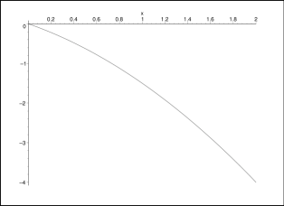
Figure 1: Typical shape of effective potential $V_{\rm eff}(\zeta)$ for unwrapped subvolume for $E>0$. The plot is for $c_{0}=1$, $c_{1}=1$, and $c_{2}=0$.

For effective potential of the internal subvolume $V_{\rm eff}(\xi)$, we have

$$d_{0} = E+\frac{D-6}{D-1}\Lambda_{D},$$

$$d_{1} = 0,$$ (57)

$$d_{2} = \frac{5(D-3)^{2}+D-6}{2(D-1)}Q_{3}^{2}.$$

We need the condition $\Lambda_{D}=-|\Lambda_{D}|<0$ and $E-\frac{D-6}{D-1}|\Lambda_{D}|<0$ as in Sec. II to have the confining behavior for large $\xi$. To have a bouncing potential for small $\xi$, we need $d_{2}>0$ and this condition is automatically is satisfied. The shape of the effective potential for this case is given in Fig. 2. The wrapped subvolume $\xi$ will oscillate around the minimum of the effective potential $\xi_{\rm min}=\sqrt{-d_{2}/d_{0}}=\sqrt{d_{2}/|d_{0}|}$.

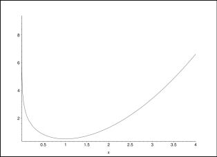
Figure 2: Typical shape of effective potential $V_{\rm eff}(\xi)$ for wrapped subvolume for $\Lambda_{D}=-|\Lambda_{D}|<0$ and $E-\frac{D-6}{D-1}|\Lambda_{D}|<0$. The plot is for $d_{0}=-1$, $d_{1}=0$, and $d_{2}=1$.

The existence of (3+1)-form RR field induces a logarithmic bounce on the effective potential of the subvolume perpendicular to it. This bounce prevents the internal subvolume from collapsing to zero size. Similarly, the existence of ($D-3+1$)-form RR field in the internal dimensions can induce nonzero logarithmic bounce for $\zeta$. However, as far as the condition $E>0$ is satisfied, the overall behavior of $\zeta$ is essentially the same (see Fig. 3).

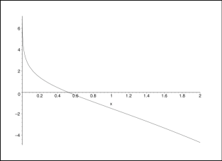
Figure 3: Typical shape of effective potential $V_{\rm eff}(\zeta)$ for unwrapped subvolume when there exists ($D-3+1$)-form RR field in the internal dimensions. The plot is for $c_{0}=1$, $c_{1}=1$, and $c_{2}=1$

IV Conclusion

In the framework of brane gas cosmology, we considered the asymmetric evolution of the universe. We showed that, provided the dilaton is stabilized by some mechanism, brane gas and RR potential can stabilize the internal dimensions. For a combination of $(D-3)$-brane gas wrapping the extra dimension and 4-form RR flux in the unwrapped dimensions, it is possible that the wrapped internal subvolume has an oscillating solution around the minimum of the effective potential while the unwrapped subvolume expands monotonically.

One key point of this paper is bulk RR field. The role of this field is to prevent the internal subvolume from collapsing to zero. It gives a logarithmic bounce to the effective potential for small values of internal subvolume. Another is the decoupling of the observed and internal dimensions by introducing an integration parameter. With this decoupling, we could treat the problem analytically in terms of two subvolumes rather than scale factors.

In our analysis we considered only brane gases for the matter part of the Einstein equation. However, there can be supergravity particles corresponding to bosonic and fermionic degrees of freedom. One can ignore the massive modes since these will decay quickly. For the massless supergravity particles, if we assume they are homogeneous and isotropic, we can take a perfect fluid form of energy momentum tensor

$$T^{M}_{N}={\rm diag}(-\rho_{\rm S},p_{\rm S},\cdots,p_{\rm S}).$$ (58)

It is well known that this term always tends to drive uniform expansion. So the main result of our analysis will not be changed even if we include the massless supergravity particles. To have more complete stabilization like the one in patil2 , where the extra dimensions are stabilized at the self-dual radius, one can include the effect of other sources. For example, including the effect of momentum modes or running dilaton may give damped oscillatory solution in which $\xi$ is driven to the minimum of the potential.

We would like to point out that the configuration in this work is just one of the possibilities to achieve the anisotropic expansion. To make anisotropic expansion between the scale factors of the observed $SO(3)$ and those of $SO(D-3)$, we considered the configuration where a gas of positive-tension $(D-3)$-branes wrap the internal dimension. An alternative way to achieve the same anisotropic expansion is to use a gas of negative-tension 3-branes wrapping the observed dimensions. Other combinations of brane gas and RR flux may give more desirable result.

References

• (1) R. Brandenberger and C. Vafa, Nucl. Phys. B 316, 391 (1989).
• (2) A. A. Tseytlin and C. Vafa, Nucl. Phys. B 372, 443 (1992); A. A. Tseytlin, Class. Quant. Grav. 9, 979 (1992).
• (3) J. polchinski, Phys. Rev. Lett. 75, 4724 (1995); E. Witten, Nucl. Phys. B 443, 85 (1995); J. polchinski, String theory (Cambridge University Press, Cambridge, England, 1998).
• (4) M. Maggiore and A. Riotto, Nucl. Phys. B 548, 427 (1999).
• (5) C. Park, S. J. Sin, and S. Lee, Phys. Rev. D 61, 083514 (2000); S. Lee and S. J. Sin, J. Korean Phys. Soc. 32, 102 (1998); C. Park and S. J. Sin, Phys. Rev. D 57, 4620 (1998); J. Korean Phys. Soc. 34, 463 (1999).
• (6) S. Alexander, R. Brandenberger, and D. Easson, Phys. Rev. D 62, 013509 (2000).
• (7) R. Brandenberger, D. A. Easson, and D. Kimberly, Nucl. Phys. B 623, 421 (2002); D. A. Easson, Int. J. Mod. Phys. A 18, 4295 (2003); M. F. Parry and D. A. Steer, J. High Energy Phys. 0202, 032 (2002); R. Easther, B. R. Greene, and M. G. Jackson, Phys. Rev. D 66, 023502 (2002); S. Watson and R. H. Brandenberger, Phys. Rev. D 67, 043510 (2003); T. Boehm and R. Brandenberger, J. Cosmol. Astropart. Phys. 0306, 008 (2003); S. H. S. Alexander, J. High Energy Phys. 0310, 013 (2003); B. A. Bassett, M. Borunda, M. Serone, and S. Tsujikawa, Phys. Rev. D 67, 123506 (2003); R. Brandenberger, D. A. Easson, and A. Mazumdar, Phys. Rev. D 69, 083502 (2004); R. Easther, B. R. Greene, M. G. Jackson, and D. Kabat, J. Cosmol. Astropart. Phys. 0401, 006 (2004).
• (8) A. Campos, Phys. Rev. D 68, 104017 (2003); R. Brandenberger, D. A. Easson, and A. Mazumdar, Phys. Rev. D 69, 083502 (2004); A. Campos, Phys. Lett. B 586, 133 (2004).
• (9) A. Kaya and T. Rador, Phys. Lett. B 565, 19 (2003); A. Kaya, Class. Quant. Grav. 20, 4533 (2003); T. Biswas, J. High Energy Phys. 0402, 039 (2004).
• (10) R. Easther, B. R. Greene, M. G. Jackson, and D. Kabat, Phys. Rev. D 67, 123501 (2003).
• (11) J. Y. Kim, Phys. Rev. D 70, 104024 (2004).
• (12) Ali Kaya, J. Cosmol. Astropart. Phys. 0408, 014 (2004); S. Arapoglu and A. Kaya, Phys. Lett. B 603, 107 (2004); T. Rador, Phys. Lett. B 621, 176 (2005); J. High Energy Phys. 0506, 001 (2005); A. Kaya, Phys. Rev. D 72, 066006 (2005); D. A. Easson and M. Trodden, Phys. Rev. D 72, 026002 (2005); A. Berndsen, T. Biswas, and J. M. Cline, J. Cosmol. Astropart. Phys. 0508, 012 (2005); S. Kanno and J. Soda, Phys. Rev. D 72, 104023 (2005); O. Corradini and M. Rinaldi, J. Cosmol. Astropart. Phys. 0601, 020 (2006); A. Nayeri, R. H. Brandenberger, and C. Vafa, Phys. Rev. Lett. 97, 021302 (2006); N. Shuhmaher and R. Brandenberger, Phys. Rev. Lett. 96, 161301 (2006); T. Biswas, R. Brandenberger, D. A. Easson, and A. Mazumdar, Phys. Rev. D 71, 083514 (2005); A. Chatrabhuti, Int. J. Mod. Phys. A 22 165 (2007); M. Borunda and L. Boubekeur, J. Cosmol. Astropart. Phys. 0610, 002 (2006).
• (13) A. Campos, Phys. Rev. D 71, 083510 (2005).
• (14) Y. K. Cheung, S. Watson, and R. Brandenberger, J. High Energy Phys. 0605, 025 (2006).
• (15) T. Battefeld and S. Watson, Rev. Mod. Phys. 78, 435 (2006).
• (16) S. P. Patil and R. Brandenberger, Phys. Rev. D 71, 103522 (2005).
• (17) S. P. Patil and R. Brandenberger, J. Cosmol. Astropart. Phys. 0601, 005 (2006).
• (18) N. Arkani-Hamed, S. Dimopoulos, N. Kaloper, and J. March-Russell, Nucl. Phys. B 567, 189 (2000); A. Riotto, Phys. Rev. D 61, 123506 (2000).