String Gas Cosmology and Structure Formation
Abstract
It has recently been shown that a Hagedorn phase of string gas cosmology may provide a causal mechanism for generating a nearly scale-invariant spectrum of scalar metric fluctuations, without the need for an intervening period of de Sitter expansion. A distinctive signature of this structure formation scenario would be a slight blue tilt of the spectrum of gravitational waves. In this paper we give more details of the computations leading to these results.
pacs:
98.80.CqI Introduction
String gas cosmology (SGC) BV ; TV (see also Perlt for early work, rbr1 ; rbr2 for recent overviews, and str for a critical review) is an approach to string cosmology, based on adding minimal but crucial inputs from string theory, namely new degrees of freedom - string oscillatory and winding modes - and new symmetries - T-duality - to the now standard hypothesis of a hot and small early universe (see others for other work on string gas cosmology, and in particular ABE for a discussion of the role which D-branes play in this scenario). One key aspect of SGC is that the temperature cannot exceed a limiting temperature, the Hagedorn temperature Hagedorn . This immediately provides a qualitative reason which leads us to expect that string theory can resolve cosmological singularities BV . From the equations of motion of string gas cosmology TV ; Ven it in fact follows that if we follow the radiation-dominated Friedmann-Robertson-Walker (FRW) phase of standard cosmology into the past, a smooth transition to a quasi-static Hagedorn phase will occur. In this phase, the string metric is quasi-static while the dilaton is time-dependent. Reversing the time direction in this argument, we can set up the following new cosmological scenario BV : the universe starts out in a quasi-static Hagedorn phase during which thermal equilibrium can be established over a large scale (a scale sufficiently large for our current universe to grow out of it following the usual non-inflationary cosmological dynamics). The quasi-static phase, however, is not a stable fixed point of the dynamics, and eventually a smooth transition to a radiation-dominated FRW phase will occur, after which point the universe evolves as in standard cosmology. This transition is connected to the decay of string winding modes into string oscillatory degrees of freedom, as described initially in BEK and studied later in more depth in Col ; Frey .
Recently Ali1 ; Ali3 it was discovered that, under certain assumptions which will be detailed below, string thermodynamic fluctuations during the Hagedorn phase lead to scalar metric fluctuations which are adiabatic and nearly scale-invariant at late times, thus providing a simple alternative to slow-roll inflation for establishing such perturbations. It is to be emphasized that this mechanism for the generation of the primordial perturbations is intrinsically stringy - particle thermodynamic fluctuations would lead to a spectrum with a large and phenomenologically unacceptable blue tilt Ali3 . As discussed in Ali2 , the stringy thermal fluctuations also generate an almost scale-invariant spectrum of gravitational waves (tensor metric fluctuations). Whereas the spectrum of scalar modes has a slight red tilt (like the fluctuations generated in most inflationary models), the gravitational wave spectrum has a slight blue tilt. This is a prediction which distinguishes our string gas cosmology scenario from standard inflationary models. In inflationary models, a slight red tilt of the spectrum is expected since the amplitude of gravitational waves is set by , and is decreasing in time, leading to lower values of when scales with larger values of the comoving wavenumber exit the Hubble radius.
In this paper, we review the analyses of our previous results Ali1 ; Ali3 ; Ali2 and present more details. The outline of this paper is as follows. We begin with a discussion of the background string gas cosmology, emphasizing the smooth transition between the initial quasi-static Hagedorn phase and the later radiation-dominated period. Next, we describe how the scalar and tensor metric fluctuations are related to correlation functions of the string gas energy-momentum tensor. In Section 4 we then discuss the computation of the string gas correlation functions. Sections 5 and 6 describe the evolution of scalar and tensor metric fluctuations, respectively. In the final section we discuss our results, point out unresolved issues and future directions for research.
In the following, we assume that our three spatial dimensions are already large (sufficiently large such that expansion according to standard cosmology beginning at a temperature of the string scale can produce our observed universe today - if the string scale is of the order GeV, then the initial size needs to be of the order of 1mm) during the Hagedorn phase (for a possible mechanism to achieve this see Natalia1 ), while the extra spatial dimensions are confined to the string scale. For a mechanism to achieve the separation into three large and six small compact dimensions in the context of SGC see BV (see however Col ; Frey for caveats), and for a natural dynamical mechanism arising from SGC to stabilize all of the moduli associated with the extra spatial dimensions see Watson ; Patil1 ; Patil2 ; Patil3 ; Edna ; shiggs (see also other2 ).
To be specific, we take our three dimensions to be toroidal. The existence of one cycles results in the stability of string winding modes - and this is a key ingredient in our calculations.
II The Background
String gas cosmology BV ; TV is based on coupling an ideal gas of strings to a dilaton-gravity background, and on focusing on the consequences which follow from the existence of new stringy degrees of freedom and new stringy symmetries, namely degrees of freedom and symmetries which are not present in point particle theories.
In the case of a homogeneous and isotropic background given by
| (1) |
the three resulting equations of motion of dilaton-gravity (the generalization of the two Friedmann equations plus the equation for the dilaton) in the string frame are TV (see also Ven )
| (2) | |||||
| (3) | |||||
| (4) |
where and denote the total energy and pressure, respectively, is the number of spatial dimensions, and we have introduced the logarithm of the scale factor
| (5) |
and the rescaled dilaton
| (6) |
If we take the spatial topology to be that of a torus with radius , the new stringy degrees of freedom are string winding modes whose energies are quantized in units of , and oscillatory modes, whose energies are independent of . The number of oscillatory modes of a string increases exponentially with energy, thus leading to a maximal temperature (the Hagedorn temperature Hagedorn ) for a gas of strings.
Since the energies of the momentum modes of a string are quantized in units of , where is the string length, the spectrum of mass states of the free string is symmetric under the interchange , the T-duality transformation. String vertex operators are also invariant under this transformation, and assuming that the symmetry extends to non-perturbative string theory leads to the existence of D-branes as new fundamental objects in string theory Pol .
In thermal equilibrium at the string scale (), the self-dual radius, the number of winding and momentum modes will be equal. Since winding and momentum modes give an opposite contribution to the pressure, the pressure of the string gas in thermal equilibrium at the self-dual radius will vanish. From the above equations of motion it then follows that a static phase will be a fixed point of the dynamical system. This phase is called the “Hagedorn phase”.
On the other hand, for large values of in thermal equilibrium the energy will be exclusively in momentum modes. These act as usual radiation. Inserting the radiative equation of state into the above equations (2 - 4) it follows that the source in the dilaton equation of motion
| (7) |
where is the equation of state parameter, vanishes and the dilaton approaches a constant as a consequence of Hubble damping. Consequently, the scale factor expands as in the usual radiation-dominated universe.
The transition between the Hagedorn phase and the radiation-dominated phase with fixed dilaton is achieved via the annihilation of winding modes, as studied in detail in BEK . The main point is that, starting in a Hagedorn phase, there will be a smooth transition to the radiation-dominated phase of standard cosmology with fixed dilaton. It is in this cosmological background that we will study the generation of fluctuations.
It is instructive to compare the background evolution of string gas cosmology with the background of inflationary cosmology Guth ; Sato , the current paradigm of early Universe evolution. Figure 1 is a sketch of the space-time evolution in string gas cosmology. For times , we are in the quasi-static Hagedorn phase, for we have the radiation-dominated period of standard cosmology. To understand why string gas cosmology can lead to a causal mechanism of structure formation, we must compare the evolution of the physical wavelength corresponding to a fixed comoving scale (fluctuations in early universe cosmology correspond to waves with a fixed wavelength in comoving coordinates) with that of the Hubble radius , where is the expansion rate. The Hubble radius separates scales on which fluctuations oscillate (wavelengths smaller than the Hubble radius) from wavelengths where the fluctuations are frozen in and cannot be effected by microphysics. Causal microphysical processes can generate fluctuations only on sub-Hubble scales (see e.g. RHBrev for a concise overview of the theory of cosmological perturbations and MFB for a comprehensive review).
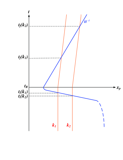
In string gas cosmology, the Hubble radius is infinite deep in the Hagedorn phase. As the universe starts expanding near , the Hubble radius rapidly decreases to a microscopic value (set by the temperature at which will be close to the Hagedorn temperature), before turning around and increasing linearly in the post-Hagedorn phase. The physical wavelength corresponding to a fixed comoving scale, on the other hand, is constant during the Hagedorn era. Thus, all scales on which current experiments measure fluctuations are sub-Hubble deep in the Hagedorn phase. In the radiation period, the physical wavelength of a perturbation mode grows only as . Thus, at a late time the fluctuation mode will re-enter the Hubble radius, leading to the perturbations which are observed today.
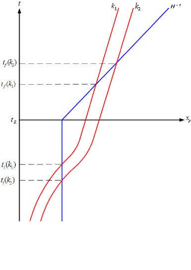
In contrast, in inflationary cosmology (Figure 2) the Hubble radius is constant during inflation (, where here is the time of inflationary reheating), whereas the physical wavelength corresponding to a fixed comoving scale expands exponentially. Thus, as long as the period of inflation is sufficiently long, all scales of interest for current cosmological observations are sub-Hubble at the beginning of inflation.
In spite of the fact that both in inflationary cosmology and in string gas cosmology, scales are sub-Hubble during the early stages, the actual generation mechanism for fluctuations is completely different. In inflationary cosmology, any thermal fluctuations present before the onset of inflation are red-shifted away, leaving us with a quantum vacuum state, whereas in the quasi-static Hagedorn phase of string gas cosmology matter is in a thermal state. Hence, whereas in inflationary cosmology the fluctuations originate as quantum vacuum perturbations Mukh ; Press , in string gas cosmology the inhomogeneities are created by the thermal fluctuations of the string gas.
As we have shown in Ali1 ; Ali3 ; Ali2 , string thermodynamics in the Hagedorn phase of string gas cosmology yields an almost scale-invariant spectrum of both scalar and tensor modes. This is an intrinsically stringy result: thermal fluctuations of a gas of particles would lead to a very different (namely very “blue” spectrum). Since the primordial perturbations in our scenario are of thermal origin (and there are no non-vanishing chemical potentials), they will be adiabatic.
III Scalar and Tensor Metric Fluctuations
In this section, we show how the scalar and tensor metric fluctuations can be extracted from knowledge of the energy-momentum tensor of the string gas.
Working in conformal time (defined via ), the metric of a homogeneous and isotropic background space-time perturbed by linear scalar metric fluctuations and gravitational waves can be written in the form
| (8) |
Here, and describe the scalar metric fluctuations. Both are functions of space and time. The tensor is transverse and traceless and contains the two polarization states of the gravitational waves. In the above, we have fixed the coordinate freedom by working in the so-called “longitudinal” gauge in which the scalar metric fluctuation is diagonal. Note that to linear order in the amplitude of the fluctuations, scalar and tensor modes decouple, and the tensor modes are gauge-invariant. Note also that in the absence of non-adiabatic stress, the two degrees of freedom and for scalar metric fluctuations coincide (see MFB for a comprehensive review of the theory of cosmological perturbations and RHBrev for a pedagogical introduction).
Inserting the above metric into the Einstein equations, subtracting the background terms and truncating the perturbative expansion at linear order leads to the following system of equations
| (9) | |||||
where , , a prime denotes the derivative with respect to conformal time , and is Newton’s gravitational constant.
In the Hagedorn phase, these equations simplify substantially and allow us to extract the scalar and tensor metric fluctuations individually. First of all, since there is no anisotropic stress at late times, and hence . Replacing comoving by physical coordinates, we obtain from the equation
| (10) |
and from the equation
| (11) |
The above equations (10) and (11) allow us to compute the power spectrum of scalar and tensor metric fluctuations in terms of correlation functions of the energy-momentum tensor. Since the metric perturbations are small in amplitude we can consistently work in Fourier space.
Our approximation scheme for computing the cosmological perturbations and gravitational wave spectra from string gas cosmology is as follows (the analysis is similar to how the calculations were performed in BST ; BK in the case of inflationary cosmology). For a fixed comoving scale we follow the matter fluctuations until the time shortly before the end of the Hagedorn phase when the scale exits the Hubble radius. At that time, we use (10) and (11) to compute the values of and ( is the amplitude of the gravitational wave tensor), and, since we are working in Fourier space, we replace the operator by .
The expectation value of the metric fluctuations is thus given in terms of correlation functions of the string energy-momentum tensor. Specifically,
| (12) |
where the pointed brackets indicate expectation values, and
| (13) |
where on the right hand side of (13) we mean the average over the correlation functions with .
After the modes exit the Hubble radius, we follow the evolution of both scalar and tensor fluctuations by means of the usual equations of cosmological perturbation theory. Apart from small corrections which arise in the time interval , this technique is justified since the dilaton is fixed after the end of the Hagedorn phase.
In the following section, we describe in a bit more detail than in our previous letters how to compute the string matter correlation functions from string thermodynamics. After that, we return to the computation of the spectrum of scalar and tensor modes.
IV Energy-Momentum Tensor Correlation Functions for Closed Strings
In the following we will denote the space-time metric by . Unlike what was done in Ali2 , we will in this paper be working with a Minkowski signature metric. The starting point for our considerations is the free energy of a string gas in thermal equilibrium
| (14) |
where is the inverse temperature and the canonical partition function is given by
| (15) |
where the sum runs over the states of the string gas, and is the energy of the state. The action of the string gas is given in terms of the free energy via
| (16) |
Note that the free energy depends on the spatial components of the metric because the energy of the individual string states does. The energy-momentum tensor of the string gas is determined by varying the action with respect to the metric:
| (17) |
Consider now the thermal expectation value
| (18) |
where and are the energy momentum tensor and the energy of the state labeled by , respectively. Making use of (17) and (16) we immediately find that
| (19) |
and hence
| (20) |
To extract the fluctuation tensor of for long wavelength modes, we take one additional variational derivative of (20), using (18) to obtain
| (21) | |||||
As we saw in the previous section, the scalar metric fluctuations are determined by the energy density correlation function
| (22) |
We will read off the result from the expression (21) evaluated for . The derivative with respect to can be expressed in terms of the derivative with respect to . After a couple of steps of algebra we obtain
| (23) |
where
| (24) |
is the specific heat, and
| (25) |
is the internal energy. Also, is the volume of the three compact but large spatial dimensions.
The gravitational waves are determined by the off-diagonal spatial components of the correlation function tensor, i.e.
| (26) |
with .
Our aim is to calculate the fluctuations of the energy-momentum tensor on various length scales . For each value of , we will consider string thermodynamics in a box in which all edge lengths are . From (21) it is obvious that in order to have non-vanishing off-diagonal spatial correlation functions, we must consisted a twisted torus. Let us focus on the component of the correlation function. We will consider the spatial part of the metric to be
| (27) |
with . The spatial coordinates run over a fixed interval, e.g. ), The generalization of the spatial part of the metric to three dimensions is obvious. At the end of the computations, we will set .
From the form of (21), it follows that all space-space correlation function tensor elements are of the same order of the magnitude, namely
| (28) |
where the string pressure is given by
| (29) |
In the following, we will compute the two correlation functions (23) and (28) using tools from string statistical mechanics. Specifically, we will be following the discussion in Deo (see also Deo1 ; Deo2 ; mb ; mt ). The starting point is the formula
| (30) |
for the entropy in terms of , the density of states. The density of states of a gas of closed strings on a large three-dimensional torus (with the radii of all internal dimensions at the string scale) was calculated in Deo (see also Ali3 ) and is given by
| (31) |
where comes from the contribution to the density of states (when writing the density of states as a Laplace transform of , which involves integration over ) from the closest singularity point to in the complex plane. Note that , and is real. From Deo ; Ali3 we have
| (32) |
In the above, is a (constant) number density of order and is the ‘Hagedorn Energy density’ of the order , and
| (33) |
To ensure the validity of Eq. (31) we demand that
| (34) |
by assuming .
Combining the above results, we find that the entropy of the string gas in the Hagedorn phase is given by
| (35) |
and therefore the temperature will be
| (36) | |||||
In the above, we have dropped a term which is negligible since (see (34)). Using this relation, we can express in terms of and via
| (37) |
In addition, we find
| (38) |
Note that to ensure that and , one should demand
| (39) |
The results (35) and (37) now allow us to compute the correlation functions (23) and (28). We first compute the energy correlation function (23). Making use of (38), it follows from (24) that
| (40) |
from which we get
| (41) |
Note that the factor in the denominator is responsible for giving the spectrum a slight red tilt. It comes from the differentiation with respect to .
Next we evaluate (29). From the definition of the pressure it follows that (to linear order in )
| (42) |
where the final partial derivative is to be taken at constant energy. In taking this partial derivative, we insert the expression (37) for and must keep careful account of the fact that depends on the radius . In evaluating the resulting terms, we keep only the one which dominates at high energy density. It is the term which comes from differentiating the factor . This differentiation brings down a factor of , which is then substituted by means of (38), thus introducing a logarithmic factor in the final result for the pressure. We obtain
| (43) |
which immediately yields
| (44) |
Note that since no temperature derivative is taken, the factor remains in the numerator. This is one of the two facts which leads to the slight blue tilt of the spectrum of gravitational waves. The second factor contributing to the slight blue tilt is the explicit factor of in the logarithm. Because of (39), we are on the large side of the zero of the logarithm. Hence, the greater the value of , the larger the absolute value of the logarithmic factor.
V Power Spectrum of Scalar Metric Fluctuations
Let us recall the philosophy behind our computation of the spectrum of scalar metric fluctuations. For a fixed comoving scale labeled by its wavenumber , we follow the energy-momentum tensor of the string matter fluctuations until the time when the scale exits the Hubble radius. At that point, we use the Einstein constraint equation (12) to determine the corresponding metric fluctuations. On super-Hubble scales for we use the usual equations for cosmological perturbations to evolve the fluctuations.
The dimensionless power spectrum of the cosmological perturbations (scalar metric fluctuations) is defined by (see e.g. Peebles )
| (45) |
where we are using the convention of defining the Fourier transform of a function including a factor of the square root of the volume of space. Thus, the dimension of is .
Making use of (12) to replace the expectation value of in terms of the correlation function of the energy density, we obtain
| (46) |
The Fourier space expectation value of is related to the position space root mean square density contrast in a region of radius via
| (47) |
and hence (46) becomes
where in the second step we have replaced the mass fluctuation by the position-space density fluctuation. According to (23), the density correlation function is given by the specific heat via , and hence (V) becomes
| (49) |
Inserting the expression from (40) for the specific heat of a string gas on a scale yields our final result
| (50) |
for the power spectrum of cosmological fluctuations.
During the Hagedorn phase, the temperature is close to the Hagedorn temperature , which in turn is given by the string scale. Thus, to a first approximation, when evaluating the spectrum (50) at the time , the temperature is independent of . Thus, the spectrum of scalar metric fluctuations is scale-invariant, with an amplitude given by
| (51) |
The last factor yields a small red tilt of the spectrum since is a slowly decreasing function of (modes with larger values of are exiting the Hubble radius later, i.e. at a slightly lower value of ).
As long as the time-dependence of the dilaton is negligible, then on super-Hubble scales the quantity which corresponds to the curvature perturbation in comoving gauge is constant (modulo effects which come from the decaying mode of at Liddle ). The quantity is defined by BST ; BK ; Lyth
| (52) |
where is the equation of state parameter.
Unlike in inflationary cosmology, where the factor changes by many orders of magnitude during reheating, in string gas cosmology makes a very mild transition between an initial value of and a final value of between the Hagedorn phase and the radiation-dominated phase. Thus, up to a factor of order unity, the conservation of on super-Hubble scales in our case leads to the conservation of .
It is important to realize, however, that in spite of the fact that the amplitude of is constant on super-Hubble scales, the fluctuation mode is evolving non-trivially - it is being highly squeezed by the expansion of the background. One way to see this is to realize that when the fluctuations cross the Hubble radius, is comparable to (since the fluctuations are thermal in origin). However, for the amplitude of decreases proportionally to . The fluctuation mode approaches the form of a standing mode at rest. This squeezing is analogous to what happens in inflationary cosmology. The only difference is that in inflationary cosmology, the squeezing takes place both during and after inflation, whereas in string gas cosmology the squeezing happens only during the period of radiation-domination.
Another way to understand the squeezing of cosmological fluctuations is in terms of canonical variables (variables characterizing the cosmological fluctuations in terms of which the action for the perturbations has canonical kinetic term). One of the key results of the quantum theory of cosmological fluctuations MFB ; RHBrev is that the variable in terms of which the action for fluctuations (for ideal gas matter) has the canonical form
| (53) |
is the so-called Sasaki-Mukhanov variable Sasaki ; Mukh2
| (54) |
where is the velocity potential of the ideal fluid, is the speed of sound, and is a function of the background given by
| (55) | |||||
The action (53) is that of a free scalar field with a time-dependent negative square mass. The mass term dominates on super-Hubble scales and leads to the squeezing of the wave function for , squeezing which is proportional to .
The squeezing of fluctuations is crucial in order to obtain the “acoustic” oscillations in the angular power spectrum of the cosmic microwave background (CMB) anisotropies SZ . If all modes enter the Hubble radius at late times as standing waves and then begin to oscillate, then at the time of last scattering the wave which is entering the Hubble radius at that time will lead to maximal redshift fluctuations, whereas a mode which has entered the Hubble radius earlier and has had time to perform oscillation will have zero amplitude and maximal velocity at , and on the corresponding angular scale the redshift contribution to the CMB anisotropies will vanish. Models without squeezing of fluctuations on super-Hubble scales do not yield this pattern of acoustic oscillations, even if they, such as in the case of topological defect models of structure formation CS , generate a scale-invariant spectrum of fluctuations.
VI Power Spectrum of Tensor Metric Fluctuations
In this section we estimate the dimensionless power spectrum of gravitational waves. First, we make some general comments. In slow-roll inflation, to leading order in perturbation theory matter fluctuations do not couple to tensor modes. This is due to the fact that the matter background field is slowly evolving in time and the leading order gravitational fluctuations are linear in the matter fluctuations. In our case, the background is not evolving (at least at the level of our computations), and hence the dominant metric fluctuations are quadratic in the matter field fluctuations. At this level, matter fluctuations induce both scalar and tensor metric fluctuations. Based on this consideration we expect that in our string gas cosmology scenario, the ratio of tensor to scalar metric fluctuations will be larger than in simple slow-roll inflationary models.
The method for calculating the spectrum of gravitational waves is similar to the procedure outlined in the last section for scalar metric fluctuations. For a mode with fixed comoving wavenumber , we compute the correlation function of the off-diagonal spatial elements of the string gas energy-momentum tensor at the time when the mode exits the Hubble radius and use (13) to infer the amplitude of the power spectrum of gravitational waves at that time. We then follow the evolution of the gravitational wave power spectrum on super-Hubble scales for using the equations of general relativistic perturbation theory.
The power spectrum of the tensor modes is given by (13):
| (56) |
for . Note that the factor multiplying the momentum space correlation function of gives the position space correlation function, namely the root mean square fluctuation of in a region of radius (the reader who is skeptical about this point is invited to check that the dimensions work out properly). Thus,
| (57) |
The correlation function on the right hand side of the above equation was computed in Section 4. Inserting the result (44) into (56) we obtain
| (58) |
which, for temperatures close to the Hagedorn value reduces to
| (59) |
This shows that the spectrum of tensor modes is - to a first approximation, namely neglecting the logarithmic factor and neglecting the -dependence of - scale-invariant. The corrections to scale-invariance will be discussed at the end of this section.
On super-Hubble scales, the amplitude of the gravitational waves is constant. The wave oscillations freeze out when the wavelength of the mode crosses the Hubble radius. As in the case of scalar metric fluctuations, the waves are squeezed. Whereas the wave amplitude remains constant, its time derivative decreases. Another way to see this squeezing is to change variables to one
| (60) |
in terms of which the action has canonical kinetic term. The action in terms of becomes
| (61) |
from which it immediately follows that on super-Hubble scales . This is the squeezing for gravitational waves.
Since there is no -dependence in the squeezing factor, the scale-invariance of the spectrum at the end of the Hagedorn phase will lead to a scale-invariance of the spectrum at late times.
Note that in the case of string gas cosmology, the squeezing factor does not differ substantially from the squeezing factor for gravitational waves. In the case of inflationary cosmology, and differ greatly during reheating, leading to a much larger squeezing for scalar metric fluctuations, and hence to a suppressed tensor to scalar ratio of fluctuations. In the case of string gas cosmology, there is no difference in squeezing between the scalar and the tensor modes. This supports our expectation that the tensor to scalar ratio will be larger in our scenario than in typical single field inflationary models. We do find a relative suppression of tensor modes, but its origin comes from string thermodynamics in the Hagedorn phase.
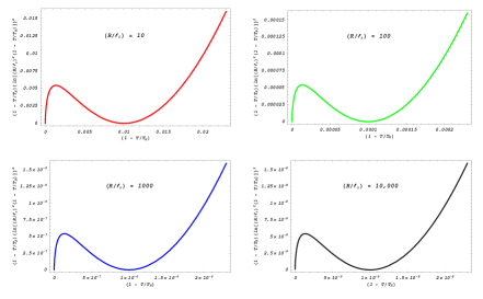
Let us return to the discussion of the spectrum of gravitational waves. The result for the power spectrum is given in (59), and we mentioned that to a first approximation this corresponds to a scale-invariant spectrum. As realized in Ali2 , the logarithmic term and the -dependence of both lead to a small blue-tilt of the spectrum. This feature is characteristic of our scenario and cannot be reproduced in slow-roll inflationary models.
To study the tilt of the tensor spectrum, we first have to keep in mind that our calculations are only valid in the range (39), i.e. to the large side of the zero of the logarithm. Thus, in the range of validity of our analysis, the logarithmic factor contributes an explicit blue tilt of the spectrum. The second source of a blue tilt is the factor multiplying the logarithmic term in (59). Since modes with larger values of exit the Hubble radius at slightly later times , when the temperature is slightly lower, the factor will be larger. Figure 3 shows the spectrum in the example of an instantaneous transition between the Hagedorn phase and the radiation-dominated period (i.e. no -dependence of ).
Note that in the result for the amplitude of the scalar metric fluctuations, the prefactor appears in the denominator and hence leads to a slight red tilt of the spectrum. In addition, the logarithmic factor is absent.
A heuristic way of understanding the origin of the slight blue tilt in the spectrum of tensor modes is as follows. The closer we get to the Hagedorn temperature, the more the thermal bath is dominated by long string states, and thus the smaller the pressure will be compared to the pressure of a pure radiation bath. Since the pressure terms (strictly speaking the anisotropic pressure terms) in the energy-momentum tensor are responsible for the tensor modes, we conclude that the smaller the value of the wavenumber (and thus the higher the temperature when the mode exits the Hubble radius, the lower the amplitude of the tensor modes. In contrast, the scalar modes are determined by the energy density, which increases at as decreases, leading to a slight red tilt.
VII Discussion
In this paper we have presented more details of the derivation of the power spectra for scalar and tensor metric fluctuations. Here we summarize the main results.
First of all, we have found that our string gas cosmology background leads to a new way of obtaining a roughly scale-invariant spectrum of cosmological perturbations. Our mechanism relies on string theory in two crucial ways. Firstly, the cosmological background is the result of a new symmetry of string theory which is not present in ordinary quantum field theory, namely T-duality. The background equations of motion which are consistent with the T-duality symmetry, namely those of dilaton gravity, predict that the radiation-dominated phase of standard cosmology was preceded by a phase - the Hagedorn phase - during which the scale factor in the string frame is static, the pressure vanishes, and the temperature is close to the limiting temperature, the Hagedorn temperature. As we have shown, string thermodynamical fluctuations in the Hagedorn phase lead to an almost scale-invariant spectrum of cosmological perturbations. This is the second point where string theory plays a crucial role. Point particle fluctuations would have given a completely different spectrum.
We have shown that the spectrum of the scalar metric fluctuations has a slight red tilt, whose value depends on how fast the transition between the Hagedorn phase and the radiation-dominated period occurs.
Our model makes a unique prediction: the spectrum of gravitational waves has a slight blue tilt, unlike the slight red tilt which is predicted in scalar field-driven inflationary models. It would be interesting to investigate how hard it would be to observationally identify this signature. One factor which will help in this regard is the fact that the tensor to scalar ratio in our scenario is not suppressed by slow-roll parameters. As can be seen immediately by comparing our results for the amplitude of the tensor and scalar power spectra, respectively, the ratio at a scale is given by
| (62) |
In principle (if the dynamical evolution from the Hagedorn phase to the radiation-dominated FRW phase were under complete analytical control) this quantity would be calculable. If the string length were known, the factor could be determined from the normalization of the power spectrum of scalar metric fluctuations. Since the string length is expected to be a couple of orders larger than the Planck length, the above factor does not need to be very small. Thus, generically we seem to predict a ratio larger than in simple slow-roll inflationary models.
We close by mentioning some limitations of our analysis. Since the dilaton is evolving until the beginning of the radiation phase, the gravitational perturbations should be determined and evolved using the complete dilaton gravity background, not using the equations of general relativity. The time dependence of the dilaton will thus lead to correction terms. We are currently in the process of calculating the magnitude of these effects. This calculation will also be crucial in order to give a correct estimate of the amplitude of the slight tilt in our spectra. These calculations are also currently in progress.
We should also emphasize that, at least in the framework presented in this paper, our cosmological scenario does not solve the entropy and flatness problems of standard cosmology. In other words, we need to start with three spatial dimensions which at the time are much larger than the string scale (the entropy problem), and we can provide no explanation for why the current universe is so close to being spatially flat. Inflationary cosmology, in addition to providing a causal mechanism for structure formation, has the potential of solving the entropy and flatness problems. On the other hand, scalar field-driven inflationary cosmology is singular, whereas string gas cosmology has the potential of providing a non-singular cosmology.
Acknowledgements.
The work of R.B. and S.P. is supported by funds from McGill University, by an NSERC Discovery Grant and by the Canada Research Chairs program. The work of A.N. and C.V. is supported in part by NSF grant PHY-0244821 and DMS-0244464.References
- (1) R. H. Brandenberger and C. Vafa, “Superstrings In The Early Universe,” Nucl. Phys. B 316, 391 (1989).
- (2) A. A. Tseytlin and C. Vafa, “Elements of string cosmology,” Nucl. Phys. B 372, 443 (1992) [arXiv:hep-th/9109048].
- (3) J. Kripfganz and H. Perlt, “Cosmological Impact Of Winding Strings,” Class. Quant. Grav. 5, 453 (1988).
- (4) R. H. Brandenberger, “Moduli stabilization in string gas cosmology,” arXiv:hep-th/0509159.
- (5) R. H. Brandenberger, “Challenges for string gas cosmology,” arXiv:hep-th/0509099.
- (6) T. Battefeld and S. Watson, “String gas cosmology,” arXiv:hep-th/0510022.
-
(7)
G. B. Cleaver and P. J. Rosenthal,
“String cosmology and the dimension of space-time,”
Nucl. Phys. B 457, 621 (1995)
[arXiv:hep-th/9402088];
M. Sakellariadou, “Numerical Experiments in String Cosmology,” Nucl. Phys. B 468, 319 (1996) [arXiv:hep-th/9511075];
D. A. Easson, “Brane gases on K3 and Calabi-Yau manifolds,” Int. J. Mod. Phys. A 18, 4295 (2003) [arXiv:hep-th/0110225];
R. Easther, B. R. Greene and M. G. Jackson, “Cosmological string gas on orbifolds,” Phys. Rev. D 66, 023502 (2002) [arXiv:hep-th/0204099];
S. Watson and R. H. Brandenberger, “Isotropization in brane gas cosmology,” Phys. Rev. D 67, 043510 (2003) [arXiv:hep-th/0207168];
T. Boehm and R. Brandenberger, “On T-duality in brane gas cosmology,” JCAP 0306, 008 (2003) [arXiv:hep-th/0208188];
R. Easther, B. R. Greene, M. G. Jackson and D. Kabat, “Brane gas cosmology in M-theory: Late time behavior,” Phys. Rev. D 67, 123501 (2003) [arXiv:hep-th/0211124];
S. Alexander, “Brane gas cosmology, M-theory and little string theory,” JHEP 0310, 013 (2003) [arXiv:hep-th/0212151];
A. Kaya and T. Rador, “Wrapped branes and compact extra dimensions in cosmology,” Phys. Lett. B 565, 19 (2003) [arXiv:hep-th/0301031];
B. A. Bassett, M. Borunda, M. Serone and S. Tsujikawa, “Aspects of string-gas cosmology at finite temperature,” Phys. Rev. D 67, 123506 (2003) [arXiv:hep-th/0301180];
A. Kaya, “On winding branes and cosmological evolution of extra dimensions in string theory,” Class. Quant. Grav. 20, 4533 (2003) [arXiv:hep-th/0302118];
A. Campos, “Late-time dynamics of brane gas cosmology,” Phys. Rev. D 68, 104017 (2003) [arXiv:hep-th/0304216];
R. Brandenberger, D. A. Easson and A. Mazumdar, “Inflation and brane gases,” arXiv:hep-th/0307043;
R. Easther, B. R. Greene, M. G. Jackson and D. Kabat, “Brane gases in the early Universe: Thermodynamics and cosmology,” arXiv:hep-th/0307233;
T. Biswas, “Cosmology with branes wrapping curved internal manifolds,” arXiv:hep-th/0311076;
A. Campos, “Late cosmology of brane gases with a two-form field,” arXiv:hep-th/0311144;
S. Watson and R. Brandenberger, “Linear perturbations in brane gas cosmology,” arXiv:hep-th/0312097;
S. Watson, “UV perturbations in brane gas cosmology,” Phys. Rev. D 70, 023516 (2004) [arXiv:hep-th/0402015];
T. Battefeld and S. Watson, “Effective field theory approach to string gas cosmology,” JCAP 0406, 001 (2004) [arXiv:hep-th/0403075];
F. Ferrer and S. Rasanen, ‘Dark energy and decompactification in string gas cosmology,” JHEP 0602, 016 (2006) [arXiv:hep-th/0509225];
M. Borunda and L. Boubekeur, “The effect of alpha’ corrections in string gas cosmology,” arXiv:hep-th/0604085. - (8) S. Alexander, R. H. Brandenberger and D. Easson, “Brane gases in the early universe,” Phys. Rev. D 62, 103509 (2000) [arXiv:hep-th/0005212].
- (9) R. Hagedorn, “Statistical Thermodynamics Of Strong Interactions At High-Energies,” Nuovo Cim. Suppl. 3, 147 (1965).
- (10) G. Veneziano, “Scale factor duality for classical and quantum strings,” Phys. Lett. B 265, 287 (1991).
- (11) R. Brandenberger, D. A. Easson and D. Kimberly, “Loitering phase in brane gas cosmology,” Nucl. Phys. B 623, 421 (2002) [arXiv:hep-th/0109165].
- (12) R. Easther, B. R. Greene, M. G. Jackson and D. Kabat, “String windings in the early universe,” JCAP 0502, 009 (2005) [arXiv:hep-th/0409121].
- (13) R. Danos, A. R. Frey and A. Mazumdar, “Interaction rates in string gas cosmology,” Phys. Rev. D 70, 106010 (2004) [arXiv:hep-th/0409162].
- (14) A. Nayeri, R. H. Brandenberger and C. Vafa, “Producing a scale-invariant spectrum of perturbations in a Hagedorn phase of string cosmology,” Phys. Rev. Lett. 97, 021302 (2006) [arXiv:hep-th/0511140].
- (15) A. Nayeri, “Inflation free, stringy generation of scale-invariant cosmological fluctuations in D = 3 + 1 dimensions,” arXiv:hep-th/0607073.
- (16) R. H. Brandenberger, A. Nayeri, S. P. Patil and C. Vafa, “Tensor modes from a primordial Hagedorn phase of string cosmology,” arXiv:hep-th/0604126.
- (17) R. Brandenberger and N. Shuhmaher, “The Confining Heterotic Brane Gas: A Non-Inflationary Solution to the Entropy and Horizon Problems of Standard Cosmology,” arXiv:hep-th/0511299.
- (18) S. Watson and R. Brandenberger, “Stabilization of extra dimensions at tree level,” JCAP 0311, 008 (2003) [arXiv:hep-th/0307044].
- (19) S. P. Patil and R. Brandenberger, “Radion stabilization by stringy effects in general relativity,” Phys. Rev. D 71, 103522 (2005) [arXiv:hep-th/0401037].
- (20) S. P. Patil and R. H. Brandenberger, “The cosmology of massless string modes,” JCAP 0601, 005 (2006) [arXiv:hep-th/0502069].
- (21) S. P. Patil, “Moduli (dilaton, volume and shape) stabilization via massless F and D string modes,” arXiv:hep-th/0504145.
- (22) R. Brandenberger, Y. K. Cheung and S. Watson, “Moduli stabilization with string gases and fluxes,” JHEP 0605, 025 (2006) [arXiv:hep-th/0501032].
-
(23)
S. Watson,
“Moduli stabilization with the string Higgs effect,”
Phys. Rev. D 70, 066005 (2004)
[arXiv:hep-th/0404177];
S. Watson, “Stabilizing moduli with string cosmology,” arXiv:hep-th/0409281. -
(24)
A. Kaya,
“Volume stabilization and acceleration in brane gas cosmology,”
JCAP 0408, 014 (2004)
[arXiv:hep-th/0405099];
A. J. Berndsen and J. M. Cline, “Dilaton stabilization in brane gas cosmology,” Int. J. Mod. Phys. A 19, 5311 (2004) [arXiv:hep-th/0408185];
S. Arapoglu and A. Kaya, “D-brane gases and stabilization of extra dimensions in dilaton gravity,” Phys. Lett. B 603, 107 (2004) [arXiv:hep-th/0409094];
T. Rador, “Intersection democracy for winding branes and stabilization of extra dimensions,” Phys. Lett. B 621, 176 (2005) [arXiv:hep-th/0501249];
T. Rador, “Vibrating winding branes, wrapping democracy and stabilization of extra dimensions in dilaton gravity,” JHEP 0506, 001 (2005) [arXiv:hep-th/0502039];
T. Rador, “Stabilization of extra dimensions and the dimensionality of the observed space,” arXiv:hep-th/0504047;
A. Kaya, “Brane gases and stabilization of shape moduli with momentum and winding stress,” Phys. Rev. D 72, 066006 (2005) [arXiv:hep-th/0504208];
D. A. Easson and M. Trodden, “Moduli stabilization and inflation using wrapped branes,” Phys. Rev. D 72, 026002 (2005) [arXiv:hep-th/0505098];
A. Berndsen, T. Biswas and J. M. Cline, “Moduli stabilization in brane gas cosmology with superpotentials,” JCAP 0508, 012 (2005) [arXiv:hep-th/0505151];
S. Kanno and J. Soda, “Moduli stabilization in string gas compactification,” ys. Rev. D 72, 104023 (2005) [arXiv:hep-th/0509074];
S. Cremonini and S. Watson, “Dilaton dynamics from production of tensionless membranes,” Phys. Rev. D 73, 086007 (2006) [arXiv:hep-th/0601082];
A. Chatrabhuti, “Target space duality and moduli stabilization in string gas cosmology,” arXiv:hep-th/0602031. - (25) J. Polchinski, String Theory, Vols. 1 and 2, (Cambridge Univ. Press, Cambridge, 1998).
- (26) A. H. Guth, “The Inflationary Universe: A Possible Solution To The Horizon And Flatness Problems,” Phys. Rev. D 23, 347 (1981).
- (27) K. Sato, “First Order Phase Transition Of A Vacuum And Expansion Of The Universe,” Mon. Not. Roy. Astron. Soc. 195, 467 (1981).
- (28) R. H. Brandenberger, “Lectures on the theory of cosmological perturbations,” Lect. Notes Phys. 646, 127 (2004) [arXiv:hep-th/0306071].
- (29) V. F. Mukhanov, H. A. Feldman and R. H. Brandenberger, “Theory Of Cosmological Perturbations. Part 1. Classical Perturbations. Part 2. Quantum Theory Of Perturbations. Part 3. Extensions,” Phys. Rept. 215, 203 (1992).
- (30) V. F. Mukhanov and G. V. Chibisov, “Quantum Fluctuation And ’Nonsingular’ Universe. (In Russian),” JETP Lett. 33, 532 (1981) [Pisma Zh. Eksp. Teor. Fiz. 33, 549 (1981)].
- (31) W. Press, Phys. Scr. 21, 702 (1980).
- (32) J. M. Bardeen, P. J. Steinhardt and M. S. Turner, “Spontaneous Creation Of Almost Scale - Free Density Perturbations In An Inflationary Universe,” Phys. Rev. D 28, 679 (1983).
-
(33)
R. H. Brandenberger and R. Kahn,
“Cosmological Perturbations In Inflationary Universe Models,”
Phys. Rev. D 29, 2172 (1984);
R. H. Brandenberger, “Quantum Fluctuations As The Source Of Classical Gravitational Perturbations In The Inflationary Universe,” Nucl. Phys. B 245, 328 (1984). - (34) N. Deo, S. Jain, O. Narayan and C. I. Tan, “The Effect of topology on the thermodynamic limit for a string gas,” Phys. Rev. D 45, 3641 (1992).
- (35) N. Deo, S. Jain and C. I. Tan, “Strings At High-Energy Densities And Complex Temperature,” Phys. Lett. B 220, 125 (1989).
- (36) N. Deo, S. Jain and C. I. Tan, “String Statistical Mechanics Above Hagedorn Energy Density,” Phys. Rev. D 40, 2626 (1989).
- (37) M. J. Bowick, “Finite temperature strings,” arXiv:hep-th/9210016.
- (38) D. Mitchell and N. Turok, “Statistical Properties Of Cosmic Strings,” Nucl. Phys. B 294, 1138 (1987).
- (39) P.J.E. Peebles, “The Large-Scale Structure of the Universe” (Princeton Univ. Press, Princeton, 1980).
- (40) S. M. Leach, M. Sasaki, D. Wands and A. R. Liddle, “Enhancement of superhorizon scale inflationary curvature perturbations,” Phys. Rev. D 64, 023512 (2001) [arXiv:astro-ph/0101406].
- (41) D. H. Lyth, “Large Scale Energy Density Perturbations And Inflation,” Phys. Rev. D 31, 1792 (1985).
- (42) M. Sasaki, “Large Scale Quantum Fluctuations In The Inflationary Universe,” Prog. Theor. Phys. 76, 1036 (1986).
- (43) V. F. Mukhanov, “Quantum Theory Of Gauge Invariant Cosmological Perturbations,” Sov. Phys. JETP 67, 1297 (1988) [Zh. Eksp. Teor. Fiz. 94N7, 1 (1988)].
- (44) R. A. Sunyaev and Ya. B. Zeldovich, “Small-Scale Fluctuations of Relic Radiation,” Astrophysics and Space Science 7, 3 (1970).
-
(45)
A. Vilenkin and E.P.S. Shellard, “Cosmic Strings and Other
Topological Defects,” (Cambridge Univ. Press, Cambridge, 1994);
M. B. Hindmarsh and T. W. B. Kibble, “Cosmic strings,” Rept. Prog. Phys. 58, 477 (1995) [arXiv:hep-ph/9411342];
R. H. Brandenberger, “Topological defects and structure formation,” Int. J. Mod. Phys. A 9, 2117 (1994) [arXiv:astro-ph/9310041].