Heisenberg honeycombs

solve Veneziano puzzle

                                                                  

A.L. Kholodenko

375 H.L.Hunter Laboratories, Clemson University, Clemson,

SC 29634-0973, USA

Abstract

In this (expository) paper and its (more technical) companion we reformulate some results of the Nobel Prize winning paper by Werner Heisenberg into modern mathematical language of honeycombs. This language was recently developed in connection with complete solution of the Horn problem (to be defined and explained in the text). Such a reformulation is done with the purpose of posing and solving the following problem: is by analyzing the (spectroscopic) experimental data it possible to recreate the underlying microscopic model generating these data? Although in the case of Hydrogen atom positive answer is known, to obtain an affirmative answer for spectra of other quantum  mechanical systems is much harder task. Development of Heisenberg’s ideas happens to be the most useful for this purpose. It supplies needed  tools to solve the Veneziano and other puzzles. The meaning of the word ”puzzle” is two-fold. On one hand, it means (in the case of Veneziano amplitudes) to find a physical model reproducing these amplitudes. On another, from the point of view of combinatorics of honeycombs, it means to find explicitly fusion rules for such amplitudes. Solution of these tasks is facilitated by our earlier developed string-theoretic formalism. In this paper only qualitative arguments are presented (with few exceptions). These arguments provide enough evidence that the underlying model compatible with Veneziano amplitudes is the standard (i.e. non supersymmetric!) QCD. In addition, usefulness of  the proposed formalism is illustrated on numerous examples such as physically motivated solution of the saturation conjecture (to be defined in the text), derivation of the Yang-Baxter and Knizhnik-Zamolodchikov equations,Verlinde and Hecke algebras, computation of the Gromov-Witten invariants for small quantum cohomology ring, etc. Finally, we discuss possible uses of these ideas in condensed matter physics

PACS: 11.25.-w; 02.20 Sv; 02.20 Uw; 02.40 Gh

MSC: 81S99; 05A17; 81R50

Subj Class.: String theory; noncommutative geometry and analysis

Keywords: honeycombs; puzzles; hives; combinatorics of complex Grassmannians; additive and multiplicative Horn problems; Littlewood-Richardson  coefficients, Gromov-Witten invariants; Knizhnik-Zamolodchikov equations; symmetric and affine symmetric groups; Hecke and Verlinde algebras;  Kashivara crystals

1 Introduction

1.1 Some general facts about Veneziano condition and its CFT analog

To avoid repetitions, we refer our readers to earlier  papers, Refs.[1-3], which shall be called Parts I-III respectively. In particular, in Part I we noticed that for the 4-particle scattering amplitude the Veneziano condition is given by

$$\alpha(s)+\alpha(t)+\alpha(u)=-1,$$ (1.1)

where $\alpha(s)$, $\alpha(t),\alpha(u)$ $\in\mathbf{Z}$ . Eq.(1.1) is a simple statement about the energy -momentum conservation. Although the numerical entries in this equation can be changed to make them more suitable for theoretical treatments, actual physical values can be subsequently re obtained by appropriate coordinate shift. Such a procedure is not applicable to amplitudes in conformal field theories (CFT) where the periodic (antiperiodic, etc.) boundary conditions cause energy and momenta to become a quasi -energy and a quasi- momenta in terminology taken from the solid state physics. Noticed differences between the  combinatorial properties of CFT and high energy physics amplitudes the major theme of this work.

To explain things better, we would like  to rewrite Eq.(1.1) in a more convenient form. Following Ref.[4], without loss of generality, the homogenous equation

$$\alpha(s)m+\alpha(t)n+\alpha(u)l+k\cdot 1=0$$ (1.2)

where $m,n,l,k$ are some integers can be added to Eq.(1.1) thus producing  the Veneziano-type equation:

$$\alpha(s)\tilde{m}+\alpha(t)\tilde{n}+\alpha(u)\tilde{l}=\tilde{k}.\text{ \ \ \ \ \ }(\text{Veneziano})$$ (1.3a)

This equation is equivalent to

$$n_{1}+n_{2}+n_{3}=\hat{N},$$ (1.3b)

where by design all entries are nonnegative integers. For the case of multiparticle scattering we anticipate that this equation is to be replaced by

$$n_{0}+\cdot\cdot\cdot+n_{k}=N$$ (1.4)

as discussed in Part II. Combinatorially, the task lies in finding all nonnegative integer combinations of $n_{0},...,n_{k}$ satisfying Eq.(1.4). It should be noted that such a task makes sense as long as $N$ is assigned. But the actual value of $N$ is not fixed and, hence, can be chosen quite arbitrarily. As explained in Part I, the value of $N$ should coincide with the exponent of the Fermat (hyper)surface if (in contrast with traditional string-theoretic treatments) we interpret Veneziano amplitudes as periods of the Fermat (hyper) surfaces living in the complex projective space. This requirement is not too rigid, however, in view of Eq.(I.3.29). Indeed, the mathematical statement of the type given by Eq.(1.4)  should be considered before the bracket operation $<$…$>$ defined in Part I is applied. This means that we shall be working mainly with the precursors of the period integrals and, therefore, we can choose any non negative integer value for $N$.Physically correct value of $N$ can then be reobtained by the appropriate coordinate shift.

In CFT such shift looses its meaning due to periodicity. In this case since the Veneziano condition, Eq.(1.3a), should be replaced by the Kac-Moody-Bloch-Bragg (K-M-B-B) condition (e.g. see Eq.(I.3.22)):

$$\alpha(s)\tilde{m}+\alpha(t)\tilde{n}+\alpha(u)\tilde{l}=mN+nN+lN\text{,\ \ \ \ (}K-M-B-B\text{)}$$ (1.5)

where $N$ is the same as before but $m,n,l$ are arbitrary integers. This circumstance  causes the energy (in free space) to become a quasi-energy (in solids). Eq.(1.5) is the most fundamental equation in X-ray crystallography [5] where it is known as the Bragg condition. In solid state physics essentially the same equation is known as the Bloch equation. As it follows from monographs by Kac [7] and, much earlier, by Bourbaki [8], the affine Lie groups and the associated with them Lie algebras are generalizations of the Weyl-Coxeter reflection groups made by analogy with crystallographic groups in solid state physics. In the language of solid state physics, the Weyl-Coxeter reflection groups are ”point” groups while the affine groups are made of semidirect products of translation groups and point groups are ”spatial” groups. Unlike the solid state physics, in the present case translations can be performed in the Euclidean, hyperbolic or spherical spaces. These spaces need not be 3 dimensional. To make a comparison with the existing literature, we shall be concerned only with the Euclidean-type translations. For a quick concise review of all these concepts we refer our readers to the Appendix A of Part II.

The arbitrariness of choosing $N$ in Eq.(1.4) represents a kind of gauge freedom. As in gauge theories, we can fix the gauge by using some physical considerations. These include, for example, an observation made in Part I that the 4-particle amplitude is zero if any two entries into Eq.(1.1) (or, which is the same, into Eq.(1.3b)) are the same. This  fact prompts us to arrange the entries in Eq.(1.3b) in accordance with their magnitudes, e.g. $n_{1}\geq n_{2}\geq n_{3}.$ More generally (in view of Eq.(1.4)), we can write: $n_{0}\geq n_{1}\geq\cdot\cdot\cdot\geq n_{k}\geq 1$. Provided that Eq.(1.4) holds, we shall call such a sequence a partition and denote it as $\mathit{\lambda}\mathit{\equiv}(n_{0},...,n_{k})$. If $\lambda$ is a partition of $N$,then we shall write $\lambda\vdash N$. It is well known from combinatorics [4,9] that there is one-to-one correspondence between the Young diagrams and partitions. We used this observation in Part II for designing new partition function capable of reproducing the Veneziano (and Veneziano-like) amplitudes. Now we would like to look at the same problem from a different angle.

1.2 The additive Horn problem

Consider some $k\times k$ Hermitian matrix $\mathcal{H}$ whose spectrum $\lambda=\{\lambda_{1}\geq...\geq\lambda_{k}\}$ can be written as a partition made of weakly decreasing sequence of $k$ real numbers. Conversely, for every spectrum $\lambda$ there is a set $\mathcal{O}_{\lambda}$ of Hermitian matrices whose spectrum   is $\lambda.$ Suppose that we are given 3 such spectra: $\lambda,\mu$ and $\nu,$ then there should be matrices $\mathcal{H}_{\lambda}\in\mathcal{O}_{\lambda},\mathcal{H}_{\mu}\in\mathcal{O}_{\mu}$ and $\mathcal{H}_{\nu}\in\mathcal{O}_{\nu}$ such that $\mathcal{H}_{\lambda}+\mathcal{H}_{\mu}=\mathcal{H}_{\nu}.$ More precisely, according to Hermann Weyl [10], the following problem can be formulated.

Problem 1.1. Assuming the eigenvalues of two $k\times k$ Hermitian matrices $\mathcal{H}_{\lambda}$ and $\mathcal{H}_{\mu}$  to be known, how does one determine all possible sets of eigenvalues for the sum $\mathcal{H}_{\lambda}+\mathcal{H}_{\mu}?$

For $k=1$ the answer is obvious but for $k>1$ the answer is much less obvious. Since $tr[\mathcal{H}_{\lambda}+\mathcal{H}_{\mu}]=tr[\mathcal{H}_{\nu}]$ we always have the trace condition:

$$\nu_{1}+...+\nu_{k}=\lambda_{1}+...+\lambda_{k}+\mu_{1}+...+\mu_{k}.$$ (1.6)

Clearly, in addition, we can expect that $\nu_{1}\leq\lambda_{1}+\mu_{1}$ since the largest eigenvalue of $\mathcal{H}_{\lambda}+\mathcal{H}_{\mu}$  is at most the sum of $\mathcal{H}_{\lambda}$ and $\mathcal{H}_{\mu}$ individual eigenvalues.

Let now I, J and K be subsets of $\{1,...,k\}$ then, what can be said about the validity of the inequality

$$\mathop{\displaystyle\sum}\limits_{i\in\mathbf{I}}\nu_{i}\leq\mathop{\displaystyle\sum}\limits_{j\in\mathbf{J}}\lambda_{j}+\mathop{\displaystyle\sum}\limits_{k\in\mathbf{K}}\mu_{k}\text{ ?}$$ (1.7)

Such type of inequalities  were analyzed by Horn [13] who formulated the following.

Conjecture 1.2. (Horn) A triple $\lambda,\mu$ and $\nu$ can represent the eigenvalues of the $\tilde{k}\times\tilde{k}$ Hermitian matrices $\mathcal{H}_{\lambda},\mathcal{H}_{\mu}$ and $\mathcal{H}_{\nu},$ where $\mathcal{H}_{\lambda}+\mathcal{H}_{\mu}=\mathcal{H}_{\nu},$ if and only if the trace condition, Eq.(1.6), holds and, in addition, the inequality given by Eq.(1.7) holds  for all sets $\{\mathbf{I},\mathbf{J}$ $and$ $\mathbf{K\}}\in T_{r}^{\tilde{k}}$ , $r<\tilde{k}.$ $T_{r}^{\tilde{k}}$ is defined recursively as follows. For each positive integer $k$ and $r\leq\tilde{k}$, let

$$U_{r}^{\tilde{k}}=\{(\mathbf{I},\mathbf{J},\mathbf{K})\mid\sum\limits_{i\in\mathbf{I}}i+\sum\limits_{j\in\mathbf{J}}j=\sum\limits_{k\in\mathbf{K}}k+r(r+1)/2\}.$$ (1.8)

In this case for $r=1$, let $T_{1}^{\tilde{k}}=U_{1}^{\tilde{k}}$ while for $r>1,$ let

$$T_{r}^{\tilde{k}} = \left\{(\mathbf{I},\mathbf{J},\mathbf{K)}\in U_{r}^{\tilde{k}}\mid\text{ \ for all }p<r\text{ and for all }(\mathbf{F},\mathbf{G},\mathbf{H})\in T_{p}^{\tilde{k}},\right.$$

$$\left.\mathop{\displaystyle\sum}\limits_{f\in\mathbf{F}}i_{f}+\mathop{\displaystyle\sum}\limits_{g\in\mathbf{G}}j_{g}\leq\mathop{\displaystyle\sum}\limits_{h\in\mathbf{H}}k_{h}+p(p+1)/2\right\}.$$

The above conjecture in principle can be checked directly using the above described recurrence. In reality, for not too large $k^{\prime}s$ the above recurrence becomes impractical. Hence, the conjecture remained unproven for about 36 years since its formulation. A complete solution was found independently by Klyachko [14] and Knutson, Tao and Woodward [15, 16] (KTW). Moreover, the infinite dimensional generalization of Klyachko results was recently obtained also by Friedland [17]. In this work we shall discuss some results of KTW since, in our opinion, they have some physical appeal. In particular, they can be used for solution of the following problem.

Problem 1.3. Is it possible to design a diagrammatic method for description of fusion algebra for the Veneziano and Veneziano-like amplitudes ?                   Stated differently, suppose we have the Veneziano (or Veneziano-like) amplitides $F(\lambda)$, $F(\mu)$ and $F(\nu),$ can we represent the product $F(\lambda)F(\mu)$ as

$$F(\lambda)\cdot F(\mu)=\mathop{\displaystyle\sum}\limits_{\nu}C_{\lambda\mu}^{\nu}F(\nu)\text{ }$$ (1.9)

with coefficients $C_{\lambda\mu}^{\nu}$  whose calculation can be completely described ? Using results by KTW we shall provide an affirmative answer to this question.

1.3 Organization of the rest of the paper

In addition to the topics already mentioned we would like to provide a summary of the content of this paper. In Section 2 we compare KTW results with those obtained much earlier by Heisenberg [18]. Although not present in textbooks on quantum mechanics, Heisenberg’s original formulation of quantum mechanics is very much in accord with that developed by KTW (who had different purposes in mind). For this reason we decided to name the KTW honeycombs ( to be introduced in Section 2) as Heisenberg honeycombs. The whole discussion of this section is motivated by the observation that the honeycomb condition(s) and Veneziano condition(s) are mathematically the same. In Section 3 we review some results from Parts II and III in order to formulate additional problems to be discussed in this (expository) paper and later, in its more technical companion, Ref.[19]. In particular, in this section we formulate problem about the fusion rules for the Veneziano amplitudes. Our discussion is not limited to these amplitudes however since combinatorially all scattering processes of high energy physics have many things in common. In the same section we argue (in accord with Parts II and III) that combinatorial considerations alone are sufficient for recovering the microscopic model leading to Veneziano and Veneziano-like amplitudes. We provide a qualitative evidence that such a model should coincide with the standard QCD leaving all details to [19]. In Section 4 we discuss actual calculations of the Littlewood-Richardson (fusion) coefficients using KTW formalism of honeycombs and puzzles. Although highly nontrivial in their design and mathematical justification, these computational tools make calculation of fusion coefficients as simple as possible and can be compared in their simplicity with Feynman’s diagrams. The advantage of utilization of such methods of calculation becomes especially apparent after we introduce and discuss the saturation conjecture and its solution in Section 5. In short, the solution of the saturation conjecture allows us to significantly enlarge number of fusion coefficients using as an input just few. Moreover, the mathematical proof of this conjecture imposes some unexpected extra constraints on fusion coefficients which can be checked experimentally. Section 6 provides necessary background for the multiplicative Horn problem to be discussed in Section 7. Section 6 is also of independent interest since it provides the most economical and physically convincing way to arrive at the classical and quantum Yang-Baxter equations, Knizhnik-Zamolodchikov equations, Dunkl operators and Hecke algebra. The multiplicative Horn problem discussed in Section 7 emerges in various physical contexts. For instance, it emerges in connection with study of solutions of Knizhnik-Zamolodchikov equations, study of spectra of quantum spin chains, study of band structure of solids, etc. Although these problems are of no immediate use for develpment of our string-theoretic formalism, they are logically compatible with this formalism and are of independent interest as we explain in Section 7. The treatment of these physically interesting problems depends upon computation of the 3-point Gromov-Witten (G-W) invariants which are structure constants of small ”quantum” cohomology ring. We enclose the word ”quantum” in quotation marks since, actually, it should be called ”double quantum” or, better, the ”deformed quantum” as we shall explain in the text. Computation of these invariants in Section 7 is non traditional in the sence that it is made for people with standard physical education (that is for people who are experts in fields other than string theory). It is hoped, that the provided background should be sufficient for proper understanding of current physical and mathematical literature on these subjects thus leading to their further uses in condensed matter physics. To keep the main text focused, some computations are presented in Appendices A through C.

2 Heisenberg Honeycomb and Veneziano condition

Following Knutson and Tao [15,16,20] (KT), we would like to describe  the construction of a honeycomb graph-a precursor of the Veneziano puzzle-which is used for calculation of $C_{\lambda\mu}^{\nu}$. In addition,  the main mathematical purpose of such a honeycomb is to provide constructive solution of the Horn conjecture. In this paper we mainly keep focus on the physical task of calculating $C_{\lambda\mu}^{\nu}$. By doing so we provide a sketch of how the Horn conjecture was solved with help of honeycombs. Details can be found in the literature already cited.

To begin, we need to work out the one dimensional example (a 1-honeycomb) in some detail in order to proceed inductively. It is helpful to replace the equation $\mathcal{H}_{\lambda}+\mathcal{H}_{\mu}=\mathcal{H}_{\nu}$ by the analogous equation $\mathcal{H}_{\lambda}+\mathcal{H}_{\mu}+\mathcal{H}_{\nu}=0,$ provided that $\lambda+\mu+\nu=0.$ Under such circumstances the inequality $\nu_{1}\leq\lambda_{1}+\mu_{1}$ is replaced by $\ 0\leq\lambda_{1}+\mu_{1}+\nu_{1}.$  Although these results are sufficient for construction of 1-honeycomb, before doing so we would like to put them in some historical perspective.

In his Nobel Prize winning paper [18] Werner Heisenberg made the following observation. Influenced by Bohr’s ideas, he looked at the famous equation for the energy levels difference:

$$\omega(n,n-\alpha)=\frac{1}{h}(E(n)-E(n-\alpha)),$$ (2.1)

where both $n$ and $n-\alpha$ are some integers. He noticed that this definition allows him to write the following  fundamental composition law

$$\omega(n-\beta,n-\alpha-\beta)+\omega(n,n-\beta)=\omega(n,n-\alpha-\beta),$$ (2.2)

or, since $\omega(k,n)=-\omega(n,k),$ the above equation can be rewritten in a more symmetric form

$$\omega(n,m)+\omega(m,k)+\omega(k,n)=0$$ (2.3)

which explains its relevance to the KT results. Most likely, being aware of Heisenberg’s unpublished letter to Krönig, Dirac in his paper, Ref.[21], of October 7th 1925 noticed that using the above combinatorial law for the frequencies in the Fourier expansions of observables leads to the multiplication rule for the Fourier amplitudes:

$$a(nm)b(mk)=ab(nk).$$ (2.4)

By noticing that, in general,

$$ab(nk)\neq ba(nk),$$ (2.5)

he concluded (in accord with Heisenberg’s  earlier cited letter) that the above multiplication rule is characteristic for matrices. Hence, the Fourier amplitudes are actually matrices! After this observation, to arrive formally at the famous quantization condition

$$[\hat{x},\hat{p}]=i\hbar$$ (2.6)

using Eq.s (2.4) and (2.5) is quite straightforward. For instance, by using the famous Dirac prescription, e.g. see Eq.(11) of his paper or his book, Ref.[22, page 86],

$$i\hbar\{x,p\}_{P.B.}=[\hat{x},\hat{p}],$$ (2.7)

where { , }_P.B. is the classical Poisson bracket. Such quantization prescription is very formal as Dirac freely admits in his paper, Ref.[21], Section 4. Its correctness is based on the historical curiosity which we discuss in detail in Section 5 in connection with physical (Heisenberg-style) solution of the saturation conjecture. In the meantime, we would like to return to Eq.(2.3) in order to analyze it from the point of view of modern mathematics.

Having in mind the KT results [15,16,20], we would like to discuss briefly some earlier efforts by Lidskii, Ref.[23], aimed at solution of the Horn conjecture. Lidskii considered $3n-1$ dimensional real vector space whose coordinates ($x_{1},...,x_{n};y_{1},...,y_{n};z_{1},...,z_{n})$ are constrained by the equation

$$\mathop{\textstyle\sum}\limits_{j=1}^{n}(x_{j}+y_{j}-z_{j})=0.$$ (2.8)

Let $W_{n}$ be a subspace of  R³ⁿ determined by the following inequalities: $x_{1}$ $\geq x_{2}\cdot\cdot\cdot\geq x_{n};y_{1}$ $\geq y_{2}\cdot\cdot\cdot\geq y_{n};z_{1}$ $\geq z_{2}\cdot\cdot\cdot\geq z_{n}.$ Furthermore, let $S_{n}$ be a subset of $W_{n}$ determined by the additional conditions. If $x=(a_{1},...,a_{n};b_{1},...,b_{n}$ ; $c_{1},...,c_{n})$ and $x\in S_{n}$, then this is possible if and only if there are linear Hermitian operators  $A,B$ and $C$ acting in $n-$dimensional complex space whose eigenvalues are $(a_{1},...,a_{n}),(b_{1},...,b_{n})$ and ($c_{1},...,c_{n})$ respectively, provided that, in addition, $A+B=C$. The problem lies in describing $S_{n}.$ Lidskii proves that $S_{n}$ is described by the inequalities given by Eq.(1.7) supplemented by the ordering requirements on $x_{i},y_{i}$ and $z_{i}$ and the Horn conditions, Eq.(1.8). According to Zelevinsky [24], Lidskii actually have not supplied a complete proof. Nevertheless, his results apparently have a stimulating effect on the KT work.

Knutson and Tao solved this problem differently in ingenious geometric way by replacing $3n-1$ space with specially chosen 2 dimensional plane in $\mathbf{R}^{3}$ defined by

$$\mathbf{R}_{\sum=0}^{3}:=\{\{x,y,z\}\in\mathbf{R}^{3}:x+y+z=0\}.$$ (2.9)

The rationale for this plane can be understood using method of induction. In one dimensional case the condition $\lambda+\mu+\nu=0$ corresponds to some particular point in $\mathbf{R}_{\sum=0}^{3}$ (which we shall  temporarily denote as $(\lambda,\mu,\nu)$ ). In their original work, Ref.[15], KT introduce both the honeycomb tinkertoys and honeycombs. The tinkertoy is some abstract directed graph placed in $\mathbf{R}_{\sum=0}^{3}$ plane whose configuration is determined by (encoded by) the honeycomb. In order to illustrate these concepts we need to establish several additional rules defining honeycombs. For instance, with each tinkertoy in $\mathbf{R}_{\sum=0}^{3}$ plane we associate another 2 dimensional (honeycomb) plane (2-plane for short) where lines can be drawn only in 3 possible directions: northeast-southwest (Ne-Sw), north-south (N-S) and northwest–southeast (Nw-Se) directions. On such 2-plane we can place a Y-shaped tripod made of nonoriented labeled semiinfinite edges as depicted in Fig.1a).The topological information encoded in such 1-honeycomb is used for construction of 1-honeycomb tikertoy, Fig.1b). The location of the vertex on such tikertoy $\mathbf{R}_{\sum=0}^{3}$ plane is determined by the condition $\bar{\lambda}+\bar{\mu}+\bar{\nu}=0$ imposed on the vectors $\bar{\lambda},\bar{\mu}$ and $\bar{\nu}$ in accord with Eq.(2.9).

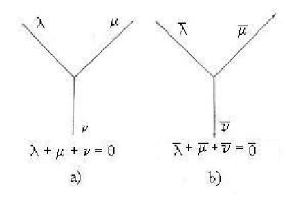
Figure 1: The 1-honeycomb a) and its 1-honeycomb tinkertoy b)

Looking at this figure more general rules for $n-$honeycombs can be developed. These are:

a) there is one-to-one correspondence between the points in $\mathbf{R}_{\mathop{\textstyle\sum}=0}^{3}$  plane

and the vertices in 2-plane;

b) there should be only finitely many vertices inside the honeycomb diagram;

c) the semiinfinite lines at the boundary of the honeycomb’s boundary are

allowed to go only in the Ne, Nw and S directions in the 2-plane.

Remark 2.1. To make sense out of the defining rules for honeycombs, our readers are encouraged to look at the following web site:

http://www.math.ucla.edu/~tao/java/Honeycomb.html
from which they can get an idea of how rules just described are implemented.

Remark 2.2 By comparing the Veneziano condition, Eq.(1.3b), with the definition of $\mathbf{R}_{\mathop{\textstyle\sum}=0}^{3}$ plane, Eq.(2.9), it is clear that the condition, Eq.(1.3b), can be brought to the form given in Eq.(2.9). Since the Heisenberg frequency condition, Eq.(2.3), is exactly the same as condition in Eq.(2.9) and since it historically was formulated much earlier, we shall call just described  honeycombs as Heisenberg honeycombs.

Assuming that our readers looked at the suggested web site, we still would like to describe some details about how these honeycombs are constructed in order to provide some sketch of KT way of solving the Horn conjecture.

Although the case of 1-honeycomb is seemingly trivial, already description of 2-honeycombs provides much more information useful for inductive analysis. The suggested web link allows our readers to recreate a 2-honeycomb and the associated with it 2-honeycomb tinkertoy. Fig.2 provides additional details.

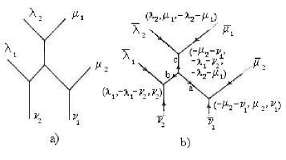
Figure 2: The 2-honeycomb a) and its 2-honeycomb tinkertoy b). The euclidean coordinates (x,y,z) of the vertices of such tinkertoy are shown explicitly

By discussing these details the rationale for keeping both the  honeycomb tinkertoys and honeycombs should become apparent. In particular, both the tinkertoy and honeycomb are uniquely determined by their boundary values, i.e. by the prescribed set ($\lambda,\mu,\nu)\equiv(\lambda_{1},\lambda_{2};\mu_{1},\mu_{2};\nu_{1},\nu_{2})$ for which the equality like that given by Eq.(1.6) is satisfied.That is we must have

$$\lambda_{1}+\lambda_{2}+\mu_{1}+\mu_{2}+\nu_{1}+\nu_{2}=0.$$ (2.10)

In addition, however, for the tinkertoy, the length of the inner edges (determined as the Euclidean distance in $\mathbf{R}_{\mathop{\textstyle\sum}=0}^{3}$ plane between the adjacent vertices) matters too. For instance, the Euclidean length of the vector b (may be, up to irrelevant factor of $\sqrt{2})$ is given by $\lambda_{1}+\mu_{2}+\nu_{1}\geq 0$ thus providing us with the 1st new nontrivial inequality. Clearly, the Euclidean lengths of vectors $\mathbf{a}$ and $\mathbf{c}$  are obtained in the same way and are given respectively by $\lambda_{2}+\mu_{1}+\nu_{1}\geq 0$ and $\lambda_{1}+\mu_{1}+\nu_{2}\geq 0.$ In view of Eq.(2.10) these inequalities can be restated as triangle inequality for the triangle made of sides whose lengths are $\lambda_{2}-\lambda_{2},\mu_{1}-\mu_{2}$ and $\nu_{1}-\nu_{2}$ respectively. Thus, the Horn conjecture in this case is solved completely by simple geometrical means. For $n>2$ the $n-$honeycomb is determined by its $3n$ boundary values ($\lambda,\mu,\nu)\equiv(\lambda_{1},...,\lambda_{n};\mu_{1},...,\mu_{n};\nu_{1},...,\nu_{n})$ subject to the constraint analogous to Eq.(2.10). In this case, however, the boundary values do not determine the $n-$honeycomb uniquely. Even though they do not determine the $n-$honeycomb uniquely, there is only finite number of different honeycombs still. Evidently, each of these more complex honeycombs will look like that depicted in Fig.3

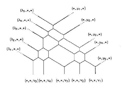
Figure 3: A typical 5-honeycomb

Already in Part I we noticed that the multiparticle Veneziano amplitude can be factorized into product of 4-particle amplitudes, e.g. see Eq.(I.3.28). Since with each such factorized amplitude we can associate a 1-honeycomb, it is only natural to expect that the higher order honeycombs can be built from an assembly of 1-honeycombs. This indeed happens to be the case and provides a compelling reason for our use of honeycombs for description of the combinatorics of Veneziano (and Veneziano-like) amplitudes.

To explain how this happens we need to pay attention to the labeling pattern , e.g. that for the 5-honeycomb depicted in Fig.3. One notices that numeration of external indices in the Ne-Sw direction goes from the bottom-up while in the Nw-Se direction-from the top-down. In the S direction the numeration goes from the right to left. This observation is essential for designing honeycombs. We would like to illustrate it by designing, say, a 4-honeycomb. For this purpose we have to assemble 4 1-honeycombs in the way depicted in Fig.4.

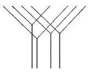
Figure 4: A precursor of a typical 4-honeycomb is made of an assembly of 4 1-honeycombs

What is depicted in this figure is still a precursor of the honeycomb. To convert this precursor into the honeycomb we need to resolve each 4-vertex into two 3-vertices as depicted in Fig.5.

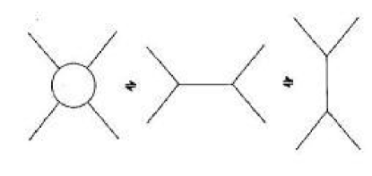
Figure 5: Resolution of a typical 4-vertex into 3-vertices

Everybody familiar with string theory at this point will be able to recognize the famous duality property depicted diagrammatically, e.g. read Ref.[25], page 265. Unlike known particle physics case, such a resolution must be performed in accord with the rules  for honeycombs defined earlier. It is also evident that the existence of such a resolution is primary cause  for the higher order honeycombs not to be determined only by the boundary values.

To illustrate these ideas we apply the rules just discussed to Fig.4 (but adopted to 2-honeycombs). In this case to make the duality of Fig.5 compatible with the rules defining honeycombs we have to give preference to only one type of resolution of 4-vertex. This fact explains why 2-honecomb is determined uniquely by its boundary data. This also explains why the higher order honeycombs are not determined by their boundary data uniquely. The honeycomb rules, although quite natural, still  are not too physically illuminating. To bring some physics into this discussion requires several steps. These are described below.

3 Complex Grassmannians  and their relation to the Veneziano-like amplitudes

3.1 Designing partition function reproducing Veneziano (and Veneziano-like) amplitudes

In Parts II and III we constructed the partition function reproducing Veneziano amplitudes. In this paper and its companion we would like to provide additional details needed for establishing firm links  between this partition function and the microscopic model, e.g. QCD.  In  Part II we used the one-to-one correspondence between partitions and the Young tableaux in order to arrive at correct result for the partition function. These simple arguments were reinforced by much deeper results taken from the theory of group invariants for pseudo-reflection groups.  In this paper we follow the same philosophy by providing simple qualitative arguments prior to more sophisticated ones.

We would like to recall some facts from Part II since they will be used later, in Section 7, when we shall discuss details of computation of the Gromov-Witten invariants. For this purpose we choose a square lattice and place on it the Young diagram (tableaux) related to some partition $\lambda$ such that $\lambda\vdash N$. To do so, we choose some $\tilde{n}\times\tilde{m}$ rectangle so that the Young diagram occupies the left part of this rectangle. We choose the upper left vertex of the rectangle as the origin of the $xy$ coordinate system whose $y$ axis (south direction) is directed downwards and $x$ axis is directed eastwards. Then, the south-east boundary of the Young diagram can be interpreted as directed (that is without self-intersections) random walk which begins at $(0,-\tilde{m})$ and ends at $(\tilde{n},0).$ Clearly, such a walk completely determines the diagram. The walk can be described by a sequence of $0^{\prime}$s and $1^{\prime}$s, say, $0$ for the $x-$step move and $1$ for the $y-$step move. We shall use a notation $\omega(\lambda)$ for such a walk so that $\omega(\lambda):=(\omega_{1}$ $,...,\omega_{N})$ where the random ”occupation” numbers $\omega_{i}=0,1$ are analogous to those used in the Fermi statistics. Evidently $\omega_{1}$ +$\omega_{2}+\cdot\cdot\cdot+\omega_{N}=\tilde{m}$. The totality $\mathcal{N}$ of Young diagrams which can be placed into rectangle is in one-to-one correspondence with the number of arrangements of 0’s and 1’s whose number $N$ is $\tilde{m}+\tilde{n}$. The logarithm of the number $\mathcal{N}$ of possible combinations of 0’s and 1’s  is just the entropy associated with the Fermi statistic (or, equivalently, the entropy of mixing for the binary mixture) used in physics literature. The number $\mathcal{N}$ is given by $\mathcal{N}=(\tilde{m}+\tilde{n})!/\tilde{m}!\tilde{n}!$. It can be represented in two equivalent ways

(3)

In Part I, Eq-s (I.1.21)-(I. 1.23)  explain how the factor $\mathcal{N}$ is entering the Veneziano amplitude. Additional significance of this number in connection with Veneziano amplitudes is discussed at length in both in Parts II and III.

Let now $p(N;\tilde{k},\tilde{m})$ be the number of partitions of $N$ into $\leq\tilde{k}$  non negative parts, each not larger than $\tilde{m}$. Consider the generating function of the following type:

$$\mathcal{F}(\tilde{k},\tilde{m}\mid q)=\mathop{\displaystyle\sum}\limits_{N=0}^{S}p(N;\tilde{k},\tilde{m})q^{N},$$ (3.2)

where the upper limit $S$ will be determined shortly below. It is shown in Refs.[3-5,9] that $\mathcal{F}(\tilde{k},\tilde{m}\mid q)=\left[\begin{array}[]{c}\tilde{k}+\tilde{m}\\ \tilde{m}\end{array}\right]_{q}$

$\equiv\left[\begin{array}[]{c}\tilde{k}+\tilde{m}\\ \tilde{k}\end{array}\right]_{q}$ where, for instance,$\left[\begin{array}[]{c}\tilde{k}+\tilde{m}\\ \tilde{m}\end{array}\right]_{q=1}=\left(\begin{array}[]{c}\tilde{k}+\tilde{m}\\ \tilde{m}\end{array}\right).$ The expression $\left[\begin{array}[]{c}\tilde{k}+\tilde{m}\\ \tilde{m}\end{array}\right]_{q}$ is a $q-$analog of the binomial coefficient $\left(\begin{array}[]{c}\tilde{k}+\tilde{m}\\ \tilde{m}\end{array}\right).$ In the literature [3-5,9] this $q-$ analog is known as the Gaussian coefficient. Explicitly,

$$\left[\begin{array}[]{c}k\\ m\end{array}\right]_{q}=\frac{(q^{k}-1)(q^{k-1}-1)\cdot\cdot\cdot(q^{k-m+1}-1)}{(q^{m}-1)(q^{m-1}-1)\cdot\cdot\cdot(q-1)}.$$ (3.3)

From this definition it should be intuitively clear that the sum defining generating function $\mathcal{F}(\tilde{k},\tilde{m}\mid q)$ in Eq.(3.2) should have only finite number of terms. Eq.(3.3) allows easy determination of the upper limit $S$ in the sum, Eq.(3.2). It is given by $\tilde{k}\tilde{m}$. This is just the area of $\tilde{k}\times\tilde{m}$ rectangle. Evidently, in view of the definition of $p(N;\tilde{k},\tilde{m})$, the number $\tilde{m}=N-\tilde{k}$. Using this fact, Eq.(3.2) can be rewritten as: $\mathcal{F}(N,N-\tilde{k}\mid q)=\left[\begin{array}[]{c}N\\ \tilde{k}\end{array}\right]_{q}.$ This expression happens to be the Poincare^′ polynomial for the complex Grassmannian $Gr(\tilde{m},\tilde{k})$. This can be found on page 292 of the famous book by Bott and Tu, Ref.[26]. From this point of view the numerical coefficients, i.e. $p(N;\tilde{k},\tilde{m}),$ in the $q$ expansion of Eq.(3.2) should be interpreted as Betti numbers of this Grassmannian. They can be determined recursively using the following property of the Gaussian coefficients [9, page 26]

$$\left[\begin{array}[]{c}n+1\\ k+1\end{array}\right]_{q}=\left[\begin{array}[]{c}n\\ k+1\end{array}\right]_{q}+q^{n-k}\left[\begin{array}[]{c}k\\ m\end{array}\right]_{q}$$ (3.4)

and taking into account that $\left[\begin{array}[]{c}n\\ 0\end{array}\right]_{q}=1.$ To connect this result with partition function reproducing Veneziano (and Veneziano-like) amplitudes we notice that, in view of relation $\tilde{m}=N-\tilde{k},$ it is more advantageous  for us to use parameters $\tilde{m}$ and $\tilde{k}$ than $N$ and $\tilde{k}$. With this in mind we obtain,

$$\left[\begin{array}[]{c}k+m\\ k\end{array}\right]_{q}$$

$$= \frac{(q^{k+m}-1)(q^{k+m-1-1}-1)\cdot\cdot\cdot(q^{m+1}-1)}{(q^{k}-1)(q^{k-1}-1)\cdot\cdot\cdot(q-1)}$$

$$= \mathop{\displaystyle\prod}\limits_{i=1}^{k}\frac{1-q^{m+i}}{1-q^{i}}\equiv\mathcal{F}(k,m\mid q).\TCItag{3.5}$$ (38)

This result is of central importance since it represents the partition function capable of reproducing the Veneziano and Veneziano-like amplitudes as we have explained at length in Parts II and III of our work. In the limit : $q\rightarrow 1,$ Eq.(3.2) reduces to the number $\mathcal{N}$ as required. To use this information in the context of honeycombs we need to remind our readers some basic facts about the Schubert calculus

3.2 Representation theory, Grassmannians, Schubert calculus and physics of orthogonal polynomials

The irreducible polynomial representations of general linear group $GL(k,\mathbf{C})$ are parametrized by the integer partitions $\lambda$ with at most $k$ parts. Given any two such polynomial representations $V^{\lambda}$ and $V^{\mu}$ one can construct the tensor product $V^{\lambda}\otimes V^{\mu}$ which is expected to be decomposable according to the rule

$$V^{\lambda}\otimes V^{\mu}=\mathop{\textstyle\sum}\limits_{\nu}C_{\lambda\mu}^{\nu}V^{\nu}$$ (3.6)

into irreducible representations $V^{\nu}$ of $GL(k,\mathbf{C}).$ Evidently, since in Eq.(1.9) the combinatorics is the same as in Eq.(3.6), the coefficients $C_{\lambda\mu}^{\nu}$ (known in literature as the Littlewood-Richardson  (L-R) coefficients) should  also be the same.

Let $\left|\lambda\right|=\lambda_{1}+...+\lambda_{k}$ then, it is known [27] that the sum in the r.h.s. of Eq.(3.6) is over partitions $\nu$ for which $\left|\lambda\right|+\left|\mu\right|=\left|\nu\right|.$ Consider the standard flag $\mathcal{F}$ of complex subspaces $\mathcal{F}$: $\mathbf{C}^{1}\subset\mathbf{C}^{2}\subset\cdot\cdot\cdot\subset\mathbf{C}^{N}$, where $N$ is related to $k$ via $k=N-m$ as before. The Schubert cell $\ \Omega_{\lambda}$ is made out of $\ k-$dimensional subspaces  $V\subset\mathbf{C}^{N}$ with prescribed dimensions of intersections with elements of $\mathcal{F}$ . More accurately, they can be described as subspaces for which $\dim(V\cap\mathbf{C}^{i})=\omega_{N}+\omega_{N-1}+\cdot\cdot\cdot+\omega_{N-i+1}$ for $i=1,2,...,m.$ Since the notion of the closure $\bar{\Omega}_{\lambda}$ for the Schubert cell is a bit technical (e.g. read page 122 of Ref.[28]) we shall skip it without much damage to physics . Such closures are called Schubert varieties. It happens, that the fundamental cohomology classes $\sigma_{\lambda}=[\bar{\Omega}_{\lambda}]$ of such varieties form a Z-basis of the cohomology ring H^∗($Gr(m,k))$ of the complex Grassmannian $Gr(m,k)$ [28-30]. The dimension of such a ring was determined in the previous subsection as $\left(\begin{array}[]{c}N\\ k\end{array}\right)$ and the multiplication rule for the product of two cohomology classes given by

$$\sigma_{\lambda}\cdot\sigma_{\mu}=\mathop{\textstyle\sum}\limits_{\nu}C_{\lambda\mu}^{\nu}\sigma_{\nu},$$ (3.7)

provided that $\left|\lambda\right|+\left|\mu\right|=\left|\nu\right|.$

The obtained correspondence can be explained based on ”physically intuitive” arguments. Indeed, if the Veneziano (and Veneziano-like) amplitudes are periods of the Fermat hypersurfaces (varieties), as explained in Part I, they should be naturally associated with the differential forms generating the cohomology ring for these varieties. When these varieties are embedded into complex projective space, where the complex Grassmannian is also embedded (via the Plücker embedding as explained in Part II), the cohomology ring for both of these varieties become interrelated. Mathematical details supporting such nonrigorous ”physical” arguments can be found in the paper by Tamvakis, Ref.[31].

The results presented above are pretty standard. We would like now to inject some physics into them.To do so, we notice that combinatorially the fusion rule, Eq.(3.7), is described with help of the Schur polynomials $s_{\lambda}(\mathbf{x})$ [32], that is (omitting the $x-$dependence) by

$$s_{\lambda}\cdot s_{\mu}=\mathop{\textstyle\sum}\limits_{\nu}C_{\lambda\mu}^{\nu}s_{\nu}.$$ (3.8)

These functions are orthogonal polynomials. That is for partitions $\mu$ and $\lambda$ and for the appropriately defined scalar product $<,>$ we obtain:

$$\left\langle s_{\lambda},s_{\mu}\right\rangle=\delta_{\lambda,\mu}.$$ (3.9)

By combining Eq.s(3.8),(3.9) we obtain as well

$$C_{\lambda\mu}^{\nu}=\left\langle s_{\lambda}\cdot s_{\mu},s_{\nu}\right\rangle,$$ (3.10a)

which, in view of Eq.(3.7), is equivalent to

$$C_{\lambda\mu}^{\nu}=\left\langle\sigma_{\lambda}\cdot\sigma_{\mu},\sigma_{\nu}\right\rangle.$$ (3.10b)

Although this result is very important from the point of view of algebraic geometry (since it describes intersection of Schubert cycles), to use it physically requires more work as we would like to explain now.

In Sections 7 and 8 of Part II we discussed why the Schur polynomials associated with KdV hierarchy (and, hence, with the Virasoro algebra (through method of coadjoint orbits) are not relevant for Veneziano amplitudes. At this point we are ready to provide additional explanation why this is so.

First, we would like to recall the definition of  one of the basic symmetric function $m_{\lambda}$ [32]. For this we have to define the monomials, e.g. x${}^{\lambda}=x_{1}^{\lambda_{1}}x_{2}^{\lambda_{2}}\cdot\cdot\cdot,$ associated with partition $\lambda.$ With thus defined monomials, $m_{\lambda}$ is just the sum of these monomials made of all possible permutations of $x^{\prime}s$. When this definition is combined with the results of Part I desribing Veneziano amplitudes as period of Fermat varieties, it should become clear that the fully symmetrized Veneziano amplitude can be obtained by using $m_{\lambda}$ in the numerator of the period integral.

Remark.3.1. It is known that $m_{\lambda}$ are eigenfunctions of the Calogero-Sutherland (C-S) model [33]. It is also known that 2 dimensional QCD is reducible to the C-S model [$34,35$]. Thus, it should be not too surprising that Veneziano amplitudes had been successful in describing scattering of mesons.

Second, since we are interested not only in Veneziano amplitudes but in general combinatorial properties of the scattering amplitudes of high energy physics, we would like to develop things a bit further. For instance, in the next subsection we shall demonstrate that combinatorial data contained in Veneziano amplitudes are quite sufficient for calculation of $C_{\lambda\mu}^{\nu}$. From this fact it is easy to make a mistake and to use the Schur polynomials $s_{\lambda}(\mathbf{x})$ in the subsequent developments. This is known and well developed pathway to the traditional string theory formalism. One should keep in mind however that, like in ordinary quantum mechanics, any symmetric function can be Fourier decomposed into Fourier series whose basis is made of orthogonal polynomials. In view of Eq.(3.9), the Schur polynomials provide a basis for such an expansion but this basis is not unique. There are other orthogonal polynomials which can be used for such a purpose [36,37]. Very much like in quantum mechanics, where all exactly solvable problems possess a complete orthogonal set of eigenfunctions, different for different problems, one can think of the corresponding exactly solvable (many-body) problems associated with orthogonal polynomials,  also different for different problems. More interesting, however, is to be able to solve the inverse problem.

Problem 3.2. For a given  set of orthogonal polynomials find the corresponding many-body operator for which such a set of orthogonal polynomials forms a complete set of eigenfunctions.

In view of the Remark 3.1., this task can be solved completely in the case of Veneziano amplitudes. In this paper and its companion we make an attempt at providing  more general outlook at solution of the Problem 3.2. We hope, that by rasing these issues more works will follow enabling to solve this problem completely.

4 Designing and solving Veneziano puzzles

4.1 General remarks

With the background just provided we are ready to connect the combinatorics of honeycombs with computation of the L-R coefficients $C_{\lambda\mu}^{\nu}$. As a by product we shall introduce another honeycomb-related construction for calculating these coefficients which KTW call a ”puzzle”[16]. Combinatorics of honeycombs is connected with the L-R coefficients in view of the following theorem, Ref.[15], page 1053.

Theorem 4.1. Let $\lambda,\mu$ and $\nu$ be three pre assigned (boundary) partitions (e.g. like those depicted in Fig.3 for the 5-honeycomb) for the $k-$honeycomb. Then the number of different honeycombs with such pre assigned boundary conditions is given by the L-R coefficient $C_{\lambda\mu}^{\nu}$

Although the above theorem hints at physical relevance of honeycombs, e.g. for practical calculation of the L-R coefficients, actual use of honeycombs for such a purpose based on the information provided is somewhat problematic. We would like to correct this deficiency now. Firstly, following KT [15], we would like to illustrate general principles by using a simple example. In particular, in the case of 3-honeycomb the decomposition of the tensor product

$$V_{(2,1,0)}\otimes V_{(2,1,0)}=V_{(4,2,0)}\oplus V_{(3,2,1)}^{\otimes 2}\oplus V_{(4,1.1)}\oplus V_{(3,3,0)}\oplus V_{(2,2,2)}$$

is graphically depicted in Fig.6.

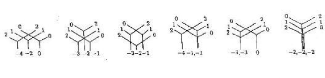
Figure 6: A typical example of a graphical calculation of the L-R coefficients with help of 3-honeycombs

Evidently, the L-R coefficients can be read off from such a decomposition straightforwardly. Moreover, as Fig.6 indicates, in actual calculations of these coefficients it is sufficient to use the precursor, e.g. see Fig.4, rather than the full blown $n-$honeycomb. This observation is especially helpful for the Veneziano (and Veneziano-like) amplitudes in view of already noticed factorization property provided by Eq.(I.3.28). It is more questionable if we are interested in the most general form of multiparticle scattering amplitude compatible with the energy-momentum conservation laws.

For the sake of such generality, we would like to discuss yet another method of computation of the L-R coefficients. This method requires designing and solving puzzles associated with honeycombs. The simplest puzzle associated with 3-honeycomb is depicted in Fig.7.

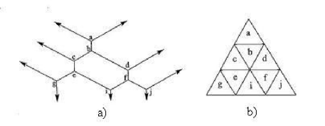
Figure 7: The labeling order of vertices of the 3-honeycomb tinkertoy a) is in one-to one correspondence with labeling of triangles (precursors of) in a puzzle b) associated with such a tinkertoy

This picture only provides a hint that honeycombs and puzzles are interconnected but not much insight into rationale for switching from honeycombs to puzzles. We would like to discuss this rationale now. For this purpose, we need to use the correspondence between the partitions and directed random walks already discussed. For each partition triple $\lambda,\mu$ and $\nu$ there is its realization in terms of such walks$:\omega(\lambda),\omega(\mu)$ and $\omega(\nu).$ Consider a particular directed random walk. It is described by the Fermi-type variable $\omega_{i}(\lambda)$ such that the constraint $\mathop{\textstyle\sum}\nolimits_{i=1}^{N}\omega_{i}(\lambda)=m=N-k$ holds. Consider now an equilateral  triangle whose sides are divided into $N$ segments of equal length. Furthermore, let  us put these segments  in correspondence with $\omega_{i}(\lambda),\omega_{i}(\mu)$ and $\omega_{i}(\nu)$, respectively for each side of the triangle. Finally, consider the set of puzzle pieces depicted in Fig.8.

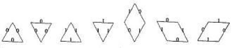
Figure 8: Basic building blocks of a puzzle

They are made of equilateral triangles and rhombi whose sides all have the same lengths equal to that of the segment on the side of the larger triangle. Since these puzzle pieces are labeled, the task is to fill in the large equilateral triangle with the puzzle pieces provided that these pieces can be rotated but not reflected when they are used to solve the puzzle. The final result looks like that depicted in Fig.9.

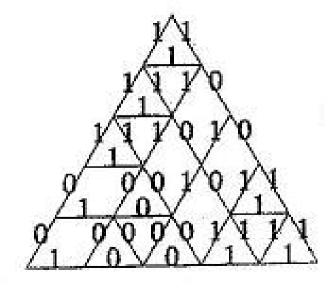
Figure 9: A typical assembled puzzle

By analogy with Theorem 4.1. it is possible to prove the following theorem.

Theorem 4.2. (Knutson-Tao-Woodward [16]) Let partitions $\lambda,\mu$ and $\nu$ be encoded by random walks $\omega(\lambda),\omega(\mu)$ and $\omega(\nu)$ whose particular realization is described in terms of 0’s and 1’s on the sides of  the equilateral triangle encoded from left to right on each of its sides in a clockwise order. Then, the number of puzzles constructed with such boundary data equals to the L-R coefficient $C_{\lambda\mu}^{\nu}$.

The easiest way to prove this theorem is through graphical bijection between the honeycombs and puzzles which we would like now to describe. At this point, in view of Fig.7, we know already that such a bijection does exist. Using results of KTW [16], it can be made more accurate now. For this purpose, the following steps should be made:

a) one should place a solved puzzle on the $\mathbf{R}_{\mathop{\textstyle\sum}=0}^{3}$ plane in such a way that the bottom right corner is at the origin. Next one should rotate this puzzle around origin by $30^{0}$ counterclockwise;

b) at each boundary segment, which is labeled by 1(1-region), attach a rhombus (outside the puzzle), then another (parallel to fist) and so on ad infimum. Fill in the rest of the plane with 0-trianges (see Fig.10);

c) deflate thus obtained extended puzzle, while keeping the right corner at the origin. The result will be the honeycomb whose vertices originate from such deflated 1-regions  and whose edges are labeled  by the thickness of the original rhombus region.

Fig.10 illustrates such described reduction procedure.

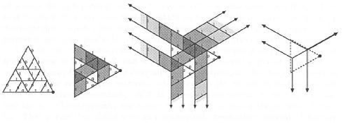
Figure 10: Successive stages of conversion of a puzzle into honeycomb

This completes our description of KTW puzzles and the associated with them Heisenberg honeycombs.

4.2 Some comments about solution of the Horn conjecture

The results described  previously are incomplete without further discussion of the Horn and saturation conjectures. In this subsection we would like to discuss some additional details related to the Horn conjecture. These may be of some importance in organizing experimental data for the mass spectrum of hadrons.

Since the case of 2-honeycombs can be solved completely, the following problem emerges.

Problem 4.3. To what extent can one use methods developed for 2-honeycombs to obtain similar type inequalities for more complex honeycombs?

We can develop our intuition by looking at Fig.4 and asking a question: is it permissible to make, say, 3-honeycomb out of 2 and 1-honeycombs as depicted in Fig.11.

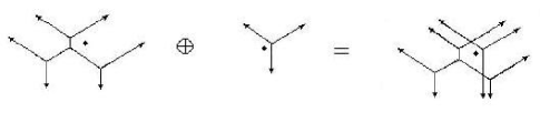
Figure 11: Designing larger honeycombs (honeycomb tinkertoys) from the smaller ones. The origin (0,0,0) is marked for each case by the black dot

Stated more formally, suppose we have $h$ and $h^{\prime}$ honeycombs what is the meaning of their direct sum $h\oplus h^{\prime}?$ If we are talking about $n-$honeycomb $h$ and $m-$honeycomb $h^{\prime},$ then the direct sum $h\oplus h^{\prime}$ must evidently correspond to the direct sum of $n\times n$ and $m\times m$ matrices combined together to form an $(m+n)\times(m+n)$ block-diagonal matrix. With such clarifications, it is possible, following KT, to give a purely geometric proof (involving $n$-honeycomb) of the inequality $\lambda_{i}+\mu_{j}+\nu_{k}\geq 0$ (known already to Weyl, Ref.[10]) provided that $i+j+k=n+2.$ For $n=1$ this inequality is obviously correct. For $n>1,$ the requirement $\ i+j+k=n+2$ should hold while in order to prove that $\lambda_{i}+\mu_{j}+\nu_{k}\geq 0,$ the ”physical” arguments can be used as follows. Consider some vertex $P$ inside the $n-$honeycomb as depicted in Fig.12.

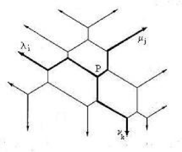
Figure 12: Using honeycomb for proving Weyl’s inequality

Next, we connect this vertex with the boundary lines marked respectively as $\lambda_{i},\mu_{j}$ and $\nu_{k}.$ Assume that our honeycomb is made of wire and assume that constant currents with intensity $\lambda_{i},\mu_{j}$ and $\nu_{k}$ are applied at the boundary lines while the rest of the boundary lines serve as sinks (i.e. they are grounded). Remembering the Kirkhoff’s rule for each vertex (that the total algebraic sum of all currents entering a given vertex must be zero) we apply this rule to the selected vertex $P$. If now the edges emanating from $P$ are labeled respectively by $\lambda_{i}^{\prime},\mu_{j}^{\prime}$ and $\nu_{k}^{\prime}$ then, the Kirkhoff rule requires: $\lambda_{i}^{\prime}+\mu_{j}^{\prime}+\nu_{k}^{\prime}=0.$ At the same time, since the current goes to other vertices too, it should be clear that: $\lambda_{i}\geq\lambda_{i}^{\prime},$ $\mu_{j}\geq\mu_{j}^{\prime}$ and $\nu_{k}\geq\nu_{k}^{\prime}.$  From here  we obtain: $\lambda_{i}+\mu_{j}+\nu_{k}\geq 0,$  in accord with Weyl. Since we would like to stay focused on our immediate (physical) tasks, we refer our readers to the already cited literature for additional details on solution of the Horn problem.

5 Solution of the saturation conjecture: from Heisenberg to Knutson and Tao and beyond

5.1 Statement of the problem

Before providing exact definitions, following KT we would like to discuss some general issues for the sake of presenting them subsequently in a proper physical context. In particular, if there exist Hermitian matrices $A,B$ and $C$ with eigenvalue sets $\lambda,\mu,$ and $\nu$ respectively, one can associate to the matrix equation $A+B+C=0$ the symbolic relation of the type

$$\lambda\boxplus\mu\boxplus\nu\sim_{c}0\Longleftrightarrow\lambda+\mu+\nu=0.$$ (5.1a)

Here the subscript $c$ means ”classical”. Although the hermiticity of matrices $A$,$B$ and $C$ makes them suitable for quantum mechanical interpretation, KT introduce another relation

$$\lambda\boxplus\mu\boxplus\nu\sim_{q}0\Longleftrightarrow\lambda+\mu+\nu=0$$ (5.1b)

where the subscript $q$ means ”quantum”. KT consider ”classical” problems as those involving Hermitian matrices with real spectrum while they consider problems as ”quantum” if the spectrum involves only integral $\lambda,\mu,$ and $\nu^{\prime}s.$ Based on these definitions, KT formulate and solve the following theorem.

Theorem 5.1. (Knutson-Tao [20]) Let $\lambda,\mu,$ and $\nu$ be weakly decreasing sequences of $n$ integers. Then, if Eq.(5.1b) holds, Eq.(5.1.a) holds as well. On another hand, if Eq.(5.1a) holds, then, there exists an integer $\ N>0$ such that $N\lambda\boxplus N\mu\boxplus N\nu\sim_{q}0\Longleftrightarrow\lambda\boxplus\mu\boxplus\nu\sim_{c}0$. (That is asymptotically, i.e. for some large $N^{\prime}s$, quantum and classical results coincide)

Based on this result KT formulate and prove the following

Conjecture 5.2. (Saturation conjecture) The above classical-quantum equivalence persist even for $N=1$.

Remark 5.3. The above conjecture can be restated in terms of the L-R coefficients $C_{\lambda\mu}^{\nu}.$ Following Fulton, Ref.[38], page 238, we expect that if $\lambda,\mu,$ and $\nu$ are a triple of partitions and $C_{N\lambda N\mu}^{N\nu}\neq 0,$ then $C_{\lambda\mu}^{\nu}\neq 0$ as well. In particular, if $C_{\lambda\mu}^{\nu}=1$ we should expect $C_{N\lambda N\mu}^{N\nu}=1$.

It should be noted, however, that in the case if $C_{\lambda\mu}^{\nu}\neq 1$ there is no reason to expect that $C_{N\lambda N\mu}^{N\nu}=$ $C_{\lambda\mu}^{\nu}.$ Since such an observation can be checked experimentally, it makes sense to discuss it in some detail in this section. Mathematically, the proof of saturation conjecture was made not only by KT but by several other authors as well . They are listed on page 238 of Ref.[38]. In this section we would like to discuss the physics of this proven conjecture based on arguments used by Heisenberg in his key paper on quantum mechanics, Ref.[18]. Some auxiliary results are presented in Appendix A.

5.2 Heisenberg’s proof of the saturation conjecture

We begin by noticing that use of Hermitian operators in quantum mechanics is motivated by the requirements that the observables which these operators represent are real numbers. In particular, for isolated stable physical system the spectrum of its eigenvalues should be real. This fact is in apparent contradiction with the KT definition of  what is ”classical” and what is ”quantum”. For instance, the famous Hydrogen atom energy spectrum is known to behave as $E_{n}\sim 1/n^{2},n=1,2,...$  The contradiction, nevertheless is only apparent. Before going into detailed explanations, we recall that famous semiclassical approximation of quantum mechanics  relates quantum results to classical in the limit of large quantum numbers. This fact can be taken as physical proof of Theorem 5.1. This makes sense only if we accept that the Hermitian operators producing real spectra have something in common with the ”classical” world.  Alternatively, we can try to prove that such a spectra cannot belong to any quantum mechanical system. Clearly, such a proof will still be insufficient to place such type of spectra into ”classical” world since in classical world there are no operators and everything commutes. Hence, we would like to approach the saturation conjecture somewhat pragmatically using physical arguments.

For this purpose, we would like to bring  to attention of our readers some important quotations from the classical book by Dirac, Ref.[22]. On page 177 of this book one reads: ” In fact it was the idea of replacing classical Fourier components by matrix elementswhich lead Heisenberg to the discovery of quantum mechanics in 1925. Heisenberg assumed that the formulas describing the interaction with radiation of a system in the quantum theory can be obtained from the classical formulas by substituting for the Fourier components of the total electric displacement of the system  the corresponding matrix elements”. Further in the text Dirac elaborates on this quantum-classical correspondence. Specifically, on pages 245-246 we read: ” Thus, the elementary theory…in which the radiation is treated as an external perturbation, gives the correct value for the absorption coefficient. This agreement between the elementary theory and the present theory could be inferred from general arguments. The two theories differ only in that the field quantities all commute with one another in the elementary theory and satisfy definite commutation relations in the present theory, and this difference becomes unimportant for strong fields. Thus the two theories must give the same absorption and emission when strong fields are concerned. Since both theories give the rate of absorption proportional to the intensity of the incident beam, the agreement must hold also for the weak fields in the case of adsorption. In the same way the stimulated part of emission in the present theory must agree with the emission in the elementary theory”.

We brought such extensive quotations from Dirac only to emphasize that, actually, at least in some cases, the quantum-classical correspondence can be pushed way down into the  seemingly quantum domain thus providing a ”proof” of the saturation conjecture. Since the existing literature on quantum mechanics (including Dirac’s book) for some reason does not discuss these issues in sufficient detail, we would like to provide such details in this section.

Following the logic of Heisenberg’s original paper, Ref.[18], Eq.(2.1), when it is treated classically, can be rewritten as

$$\omega(n,\alpha)=\alpha\omega(n)\simeq\alpha\frac{1}{\hbar}\frac{\partial E}{\partial n}.$$ (2.1a)

Next, Heisenberg notices that, actually, the famous Bohr-Sommerfeld (B-S) quantization rule

$$\oint pdq=nh,\text{ }n=0,1,2,...,$$ (5.2)

is not exact ! It is determined only with accuracy up to some constant (unknown at the time of  his writing). He argues, that if such a constant would be known, this rule would become exact, that is valid for any $n$’s. From the point of view of our present understanding of quantum mechanics his intuition was correct: the old fashioned Bohr-Sommerfeld rule is valid rigorously in the limit of large $n$’s while the calculation of the constant can be done, for instance, with help of either the WKB or of  much more sophisticated  theory of Maslov index [39]. These arguments although plausible are superficial nevertheless as can be found from the book by Arnold, Ref.[40], page 246. From it we find that already at the classical level the adiabatic invariant $\oint pdq$ is determined only with accuracy up to some constant. This observation makes Heisenbeg’s arguments less convincing.

In particular, following Heisenberg we claim that if the B-S quanization rule, when corrected, makes sense fully quantum mechanically, one can get, in principle, the additional information out of it. For this purpose Heisenberg introduces the Fourier decomposition of the generalized coordinate $q$, i.e.

$$q(n,t)=\sum\limits_{\alpha=-\infty}^{\infty}a_{\alpha}(n)\exp(i\omega(n,\alpha)t)$$ (5.3)

where we used Eq.(2.1a) thus causing us to keep our calculations with respect to the some pre assigned energy level $n$ (e.g. see Appendix A). The velocity can be readily obtained now as

$$\dot{q}(n,t)=\sum\limits_{\alpha=-\infty}^{\infty}ia_{\alpha}(n)\omega(n,\alpha)\exp(i\omega(n,\alpha)t)$$ (5.4a)

so that calculation of the velocity square averaged over the total period is given by

$$\oint\left[\dot{q}(n,t)\right]^{2}dt=2\pi\sum\limits_{\alpha=-\infty}^{\infty}\left|a_{\alpha}(n)\right|^{2}\omega(n,\alpha)^{2}.$$ (5.4b)

At this point it should be noted that the original of Heisenberg’s paper, Ref.[18], contains (perhaps) a typographical error: instead of having $\omega(n,\alpha)^{2}$ Heisenberg writes $\omega(n,\alpha).$ This fact was noticed by the editors of his collected papers, Ref.[18]. Now we use this result in the B-S quantization rule, i.e. we have

$$\oint pdq=\oint m\dot{q}dq=\oint m\dot{q}^{2}dt=2\pi m\sum\limits_{\alpha=-\infty}^{\infty}\left|a_{\alpha}(n)\right|^{2}\omega(n,\alpha)^{2}=nh+const.$$ (5.5)

Next, Heisenberg argues as follows. Since the const is unknown, it is of interest to obtain results which are constant-independent. At the same time, since the result, Eq.(5.5), is assumed to be exact, we have to use instead of scalars $\left|a_{\alpha}(n)\right|^{2}$ the matrices in accord with Eq.(2.4). This would lead us to matrices of the type $\left|a(n,n+\alpha)\right|^{2}$ and $\left|a(n,n-\alpha)\right|^{2}$ depending on the actual sign of $\alpha.$ In addition, he silently  had assumed that the $n-$dependence of the amplitudes is much weaker than that for the frequencies $\ \omega(n,n+\alpha)$ and $\omega(n,n-\alpha)$ so that it can neglected completely. Under such conditions he treats $n$ as continuous variable and differentiates both sides of Eq.(5.5) with respect to $n$ thus obtaining (recall that $\omega(mn)=-\omega(nm)):$

$$h=4\pi m\sum\limits_{\alpha=0}^{\infty}\{\left|a(n,n+\alpha)\right|^{2}\omega(n,n+\alpha)-\left|a(n,n-\alpha)\right|^{2}\omega(n,n-\alpha)\}.$$ (5.6)

The validity of this result depends upon the additional assumption about the ground state energy. If $n_{0}$ represents such a state, then one must require that

$$a(n_{0},n_{0}-\alpha)=0\text{ \ }\forall\alpha>0.$$ (5.7)

In Ref.[18] Heisenberg acknowledges that this result was inspired by the earlier result of Kramers who calculated the induced dipole moment of electrons in atom assuming rules of quantum mechanics (in fact before it was officially inaugurated !), e. g. see Appendix A. Results of the Appendix A then lead us directly to the famous commutation rule

$$[\hat{x},\hat{p}]=i\hbar.$$ (5.8)

Heisenberg argues that his reasonings are correct since the frequency of the incoming (scattered) light is much higher than that for characteristic ”rotational” frequencies in the atom so that the electrons can be treated as ”free” and independent.

The discussion we just presented is aimed to underscore the differences between physical reality and mathematical correctness. It can be considered as the Heisenberg-style proof  of the saturation conjecture and provides us with rationale for discussion of an alternative formulation of quantum mechanics (to be presented in the next section). Before doing so we would like to discuss the saturation conjecture and its proof in connection with results of our earlier published Parts II and III. This will enable us to make some physical sense out of recently obtained mathematically interesting results.

5.3 Combinatorics of L-R coefficients and the Ehrhart polynomial

In this subsection we would like to address the following problem: suppose we are given a L-R coefficient $C_{\lambda\mu}^{\nu}$, can this information be used for calculation of $C_{N\lambda N\mu}^{N\nu}?$ Although calculations of L-R coefficients have a rather long history [41], the full answer to this question was obtained only quite recently in connection with positive solution of the saturation conjecture. It should be noted that although the attempts in this direction were made a bit earlier by Berenstein and Zelevinsky [42], the actual numerical results were obtained much later by King et al [43]. These authors were inspired by the results of KT, Refs.[15,16], where, in addition to the honeycomb model, the hive model was introduced which we have not discussed thus far. An n-hive is a triangular array of numbers $a_{ij}$ with $0\leq i,j\leq n$. Say, for $n=4$ a typical arrangement looks as follows

$\begin{array}[]{ccccccccc}&&&&a_{00}&&&&\\ &&&a_{10}&&a_{01}&&&\\ &&a_{20}&&a_{11}&&a_{02}&&\\ &a_{30}&&a_{21}&&a_{12}&&a_{03}&\\ a_{40}&&a_{31}&&a_{22}&&a_{13}&&a_{04}\end{array}$

Such an $n-$hive is an integer hive if all of its entries are non-negative integers. The numbers $a_{ij}$ in the hive are subject to the hive conditions given symbolically  by R1: $\begin{array}[]{ccc}a&b&\\ &c&d\end{array};$ R2: $\begin{array}[]{ccc}&a&\\ b&&c\\ &d&\end{array}$ and R3: $\begin{array}[]{ccc}&b&d\\ a&c&\end{array}$ implying $b+c\geq a+d$ for $a,b,c$ and $d$ being the neighboring entries in the $n-$hive. We shall call such type of inequalities the hive condition (HC). Based  on these results, the following definition can be made

Definition 5.4. A L-R hive is an integer hive satisfying the HC for all constituent rhombi R1-R3. For such a hive the border entries are determined by partitions $\lambda,\mu$ and $\nu$ in such a way that $a_{00}=0,a_{0j}=\lambda_{1}+\lambda_{2}+...+\lambda_{j\text{ }},j=1,2,...,n,a_{i0}=\nu_{1}+\nu_{2}+...+\nu_{i},i=1,2,...,n,a_{k,n-k}=a_{0n}+\mu_{1}+\mu_{2}+...+\mu_{k}$ , $k=1,2,...,n$, provided that $\left|\lambda\right|+\left|\mu\right|=\left|\nu\right|$ and the number of parts ${l}$($\lambda),{l}(\mu)$ and l($\nu)$in partitions $\lambda,\mu$ and $\nu$ is bounded by $n$.

Based on this definition, and motivated by Theorems 4.1. and 4.2. Fulton [44] proved the following theorem

Theorem 5.5. The L-R coefficient $C_{\lambda\mu}^{\nu}$ is the number of LR hives with border labels determined by $\lambda,\mu$ and $\nu.$

Alternative (simpler) proof of this theorem as well as many other useful results can be found in the recent paper by Pak and Vallejo [45]. In both cases the proof is based on careful solution of the rhombus constraints (or HC) for the integer hives. In the case of $n$-hive there are $m=(n-1)(n-2)/2$ interior vertex labels for $a_{ij}$.The corresponding set of linear constraints with integer coefficients defines a convex rational (not integral! as in Part III) (hive) polytope $\mathcal{P}$ living in R${}^{m}.$ As in Part III we can define the Ehrhart polynomial $\mathfrak{P}$($N$, m) for such polytope and the associated with it generating (partition) function $\mathcal{F}(\mathcal{P},x)$ via

$$\mathcal{F}(\mathcal{P},x)=\mathop{\textstyle\sum}\limits_{N=0}^{\infty}\mathfrak{P}\mathit{(}N\mathit{,\ m)x}^{N}.$$ (5.9)

In the present case, $\mathfrak{P}\mathit{(}N\mathit{,\ m)=}C_{N\lambda N\mu}^{N\nu}$ . Unlike the integral polytope $\mathcal{P}$ for which the generating function $\mathcal{F}(\mathcal{P},x)$ can be written in closed form given by Eq.(III.1.14), in the present case, since the polytope is only rational (that is not all of its vertices lie at the nodes of Z${}^{m})$, such closed form universal result for $\mathcal{F}(\mathcal{P},x)$ cannot be used. Using method of quivers, Derksen and Weyman [46] were able to prove that, nevertheless, the universal form given by Eq.(III.1.14) still holds (provided that the dimensionality $m$ of the lattice Z^m is replaced by m̃ and the indeterminate $x$ is replaced by $x^{\alpha}$ where both $\tilde{m}$ and $\alpha$ are some known (in principle) nonnegative integers.

In view of such an interpretation of stretched L-R coefficients, the whole chain of arguments of Part III can be used practically unchanged. This makes Eq.(III.4.30) especially relevant demonstrating that combinatorics of the L-R coefficients can be obtained field-theoretically in the spirit of earlier treated Witten-Kontsevich model [47]. These results will be extended further in Section 7 in which we discuss (among other things) the Gromov-Witten invariants.

Remark 5.6. Obtained connections between the L-R coefficients $C_{\lambda\mu}^{\nu}$ and their inflated counterparts $C_{N\lambda N\mu}^{N\nu}$ is very important from the experimental point of view. Indeed, by looking at Eq.(1.4) and recalling its relevance to Veneziano amplitudes described in Parts II and III, one would naively expect that for any $N$ one should have $C_{\lambda\mu}^{\nu}=C_{N\lambda N\mu}^{N\nu}$ . Mathematics tells us that this may happen only if $C_{\lambda\mu}^{\nu}=1.$ It remains to check experimentally if the constraint $C_{\lambda\mu}^{\nu}=1$ is a valid physical constraint. These arguments clearly not restricted to the Veneziano-type amplitudes and should be taken into account for any amplitude of high energy physics.

Problem 5.7. In the case if the hypothetical scattering processes requires use of supersymmetric QCD, how supersymmetry can be detected through study of  combinatorics of experimental data, say, of the LR fusion coefficients ?

6 From Heisenberg back to Maxwell,Tait and Kelvin

6.1 General remarks

In view of the results of previous section and those of the Appendix A we would like to formulate the following problem

Problem 6.1. Given the experimental origin (discussed in Appendix A) and the associated with it inevitable computational approximations leading to the basic commutation rule, Eq.(5.8), is it possible to develop quantum mechanics without this rule being put at its foundation? Alternatively said, can we recover this basic rule without use of light scattering experiments and the B-S quantization rule?

Remark 6.2. Since all experimental data for any quantum mechanical system (atom, molecule, solid, etc.) are spectroscopic in nature we know about the system as much as the combinatorics of experimental data provides. From such point of view there is not much difference between, say, biological problems, computer science problems, astrophysical problems, etc. and those in the high energy physics.

A superficial answer to just posed problem can be made like this: should the above rule be wrong we would not be able to recover the spectrum of Hydrogen atom with such an amazing accuracy using established methods of quantum mechanics. This remarkable agreement between theory and experiment is possible only if such commutation rule is correct. Clearly, it is correct! Nevertheless, we can still argue against its up-front use as follows. Heisenberg uses the  B-S quanization rule (perhaps adjusted) to obtain his results. This rule makes sense only if classically there is a complete separation of variables done with help of the Hamilton-Jacobi formalism. When this happens, the system is considered to be completely integrable. Hence, any completely integrable system is just the set of independent harmonic oscillators. The Hydrogen atom is surely a good candidate for such procedures but what about the Helium ? The B-S rule cannot be applied strictly speaking already to the Helium so that Heisenberg’s chain of reasoning leading to the commutator, Eq.(5.8), formally breaks down. Besides, since the B-S quantization cannot be used for spin quantization (since formally there is no classical analog of spin, i.e. B-S rule does not account for the half integers), the spin has no place in the Schrödinger’s formalism. Since Schrödinger have demonstrated the equivalence of his formalism to that developed by Heisenberg as described in Dirac’s book, Ref.[22], apparently, there is no room for the spin in the Heisenberg formalism as well. Surely, this happens to be only apparently true as we would like to explain now. In doing so we do not need to use the relativistic formalism developed by Dirac.

6.2 Heisenberg’s paper revisited

We begin with discussion of some consequences of Heisenberg’s results following  the1925 paper by Dirac, Ref.[21]. We selected this paper in view of its remarkable completeness: all quantum mechanical formalism used today can be traced back to this paper. Dirac acknowledges, though, that his paper was written as consequence of Heisenberg’s results. In particular, the famous Dirac quantization rule, Eq.(2.7), is just restatement of the results by Heisenberg. As good as it is, its use is questionable in general. Indeed, in comments to his Eq.(11) Dirac states that the difference of Heisenberg’s products of two quantum observables $x$ and $y$ is equal to the (classical!) Poisson bracket of their classical counterparts multiplied by $\frac{ih}{2\pi}$ or, symbolically,

$$\hat{x}\hat{y}-\hat{y}\hat{x}=\frac{ih}{2\pi}\{x,y\}_{p.b.}$$ (6.1)

This expression makes sense for $x\leftrightarrows\hat{x}$ and $y\leftrightarrows\hat{p}$ . But, in general, for arbitrary classical observables $x$ and $y$  we are dealing with the Lie algebra which requires this Poisson bracket to be expanded into linear combinations of classical obseravbles so that the l.h.s and the r.h.s of Eq.(6.1) do not match. Hence, we come back to the Heisenberg-Kramers result presented in the Appendix A as the only justification. This difficulty was recently noticed and discussed in the book by Adler who suggests to treat classical Poisson bracket quantum mechanically in the style of Heisenberg, e.g. see Eq.(1.13b) of Ref.[52].

In this paper, we choose another way to by pass the Heisenberg-Dirac quantization prescription. For this purpose, we would like to make few additional comments regarding traditional formulations. Following Dirac we introduce the evolution operator $U(t)$ bringing the initial state wave function $\psi_{0}$ to its final state $\psi(t),$ i.e. $\psi(t)=U(t)\psi_{0}.$ For the time-independent Hamiltonian $\hat{H}$ the formal solution of the Schrödinger-type equation

$$i\hbar\frac{d}{dt}\hat{U}^{-1}(t)=\hat{H}\hat{U}^{-1}(t)$$ (6.2)

is known to be given by $\hat{U}^{-1}(t)=\exp(-\frac{i}{\hbar}\hat{H}t).$ Now, Heisenberg considered the quantum Fourier transform by replacing the usual Fourier amplitudes by matrices, i.e. he used quantities like $a(mn)exp(\frac{i}{\hbar}\omega(mn)t).$ In the modern language this can be rewritten as follows. Let $\hat{O}$ be some quantum mechanical operator whose evolution is described by $\hat{U}(t)\hat{O}\hat{U}^{-1}(t)=\hat{O}(t).$ This operator leads to the matrix elements : $<m\mid\hat{O}\mid n>exp(\frac{i}{\hbar}\omega(mn)t)$ with $\omega(mn)$ defined by Eq.(2.1) with $<m\mid$ and $\mid n>$ being time-independent wave functions of the Hamiltonian $\hat{H}$. Clearly, if the observable $\hat{O}(t)$ is an identity element in the algebra of observables, we obtain : $<m(t)\mid$ $n(t)>=<m\mid n>,$ where $\mid n(t)>=U(t)\mid n>.$ The requirement for the observables to be real leads to the Hermitian type operators whose eigenfunctions are mutually orthogonal.  Under such conditions we may or may not require these mutually orthogonal functions to be normalized to 1. By doing so we do not insist on the probabilistic interpretation of quantum mechanics. Such an interpretation emerges anyway within quantum statistical mechanics.

In view of earlier posed Problem 6.1. it makes sense to replace the Dirac quantization rule, Eq.(6.1), by the requirement of orthogonality for the wave functions. Under such a rule we need to have a supply of orthogonal functions (if the spectrum is countably infinite) or orthogonal basis in some complex finite dimensional vector space. In the case of orthogonal functions, it is known that all one variable orthogonal functions used in quantum mechanical exactly solvable problems are obtainable from the one variable Gauss-type hypergeometric functions [53]. These functions are expressible in the form of period integrals. The Veneziano and Veneziano-like scattering amplitudes considered in Part I belong to the same family of hypergeometric- type period integrals  initially considered by Aomoto [54] and subsequently by many others [55]. The cohomological meaning of such integrals is explained in detail in Ref.[56]. By the  principle of complementarity all many-body exactly solvable quantum mechanical problems should be related to the hypergeometric functions of multiple arguments. More importantly for us is that these hypergeometric functions produce sets of all known orthogonal polynomials replacing one-variable orthogonal functions of usual quantum mechanics. Hence, they are also period integrals. A nice summary of developments in this area can be found in Refs.[57,58].  The finite dimensional cases (including spin)  technically present no difficulties under such circumstances.

At this stage we are ready to provide additional  arguments in support of our point of view on quantum mechanics. These arguments will be also of use in the next section. Traditionally, in the Heisenberg interpretation of quantum mechanics equations of motion for the operators $\hat{O}_{i}(t)$ can be obtained by simple differentiation of $\hat{U}(t)\hat{O}_{i}\hat{U}^{-1}(t)=\hat{O}_{i}(t)$. This procedure formally leads to the Heisenberg’s equation of motion

$$i\hbar\frac{\partial\hat{O}}{\partial t}=[\hat{O},\hat{H}]$$ (6.3)

for the operator $\hat{O}$. The rationale for such writing comes from the analogy of this equation with that known in classical Hamiltonian mechanics. This makes sense only if the Dirac quantization prescription makes sense. But it does not as we just discussed! Instead of repairing this situation using known mathematical methods of geometric quantization [60,61], we follow Heisenberg’s philosophy based on careful analysis of spectroscopic data. From his point of view we have the set of classical observables $\{O_{i}(t)\}$ which is supposedly complete. This means that treating the Poisson brackets as Lie brackets we have

$$\{O_{i},O_{j}\}=\sum\limits_{k}C_{ij}^{k}O_{k}.$$ (6.4)

Accordingly, quantum mechanically, instead of Eq.(6.3) we need to consider the result

$$[\hat{O},\hat{H}]=\sum\limits_{k}\tilde{C}_{oh}^{k}\hat{O}_{k}$$ (6.5)

valid for any $t$! So that under such circumstances (quantum) dynamics formally disappears! This observation can be strengthened due to the following chain of arguments. In mathematics (see Part III, Section 3.2) expression like $\hat{U}(t)\hat{O}_{i}\hat{U}^{-1}(t)=\hat{O}_{i}(t)\equiv Ad_{\hat{U}}\hat{O}_{i}$ defines an orbit for the operator $\hat{O}_{i}$ in the Lie algebra (made of operators $\{\hat{O}_{i}\})$ caused by the action of elements $\hat{U}$ from the associated with it Lie group. At the same time, the mathematics of Lie groups and Lie algebras produces for $[\hat{O},\hat{H}]$= $\mathit{ad}_{\hat{H}}\hat{O}$ where both $\hat{O}$ and $\hat{H}$ are in the Lie algebra $\{\hat{O}_{i}\}.$Evidently, we can obtain the same (or even greater) information working with $Ad$ operators instead of $ad$. In particular, we would like to consider the trace, i.e. tr{$Ad_{U}\hat{O}_{i}\}=\chi(\hat{O}_{i}),$ which is just the character for $\hat{O}_{i}$. Clearly, it is time-independent. If this is so, then, what is the meaning of an orbit ? This  topic was discussed at length in Parts II and III of our work. To avoid repetitions we refer our readers to these papers.  If there is no time evolution for the character, superficially, nothing happens. This is not true, however as was recognized already by Dirac, Ref.[22]. In Chapter 9 he writes: ” The Hamiltonian is a symmetrical function of the dynamic variables and thus commutes with every permutation. It follows that each permutation is a constant of motion. This happens even if the Hamiltionian is not constant.” Hence, the orbit $Ad_{\hat{U}}\hat{O}_{i}$ is caused by permutations. These can be analyzed with help of the torus action thus leading to the Weyl-Coxeter reflection group $W=N/T$ described in Section 3.1 of Part III and to the associated with them Lie algebras discussed in section 3.2. of Part III. Representations of these Lie algebras  (including the affine Lie algebras) produce all known quantum mechanical results as well as those of conformal field theories (CFT). This was explained in Part III. At this point we would like to do more.

6.3 Symmetric group and its relatives

As is well known, the symmetric group $S_{n}$ has the following presentation in terms of generators $s_{i}$ and (Coxeter) relations

$$s_{i}^{2} = 1$$

$$s_{i}s_{j} = s_{j}s_{i\text{ }}\text{for }\left|i-j\right|\geq 2,$$

$$s_{i}s_{i+1}s_{i} = s_{i+1}s_{i}s_{i+1}.\TCItag{6.6}$$ (53)

If there is a set of $n$ elements (say, the Weyl roots arranged in a certain order) the generator $s_{i}$ interchanges an element $i$ with $i+1$ so that $s_{1},...,s_{n-1}$ generate $S_{n.}$Clearly, there are $n!$ permutations in the set of $n$ elements. If we assign the initial ordered state, then any other state can be reached by successful application of permutational generators to this state so that the word $w=s_{a_{1}}s_{a_{2}}\cdot\cdot\cdot s_{a_{l}}$ (where the indices $a_{1},...,a_{l}$ represent a subset of the set of $n-1$ elements) can be identified with such a state. Since one can reach this state in many ways, it makes sense to introduce the reduced word $w$ whose length $\mathit{l(w)}$ is minimal. With these definitions, we would like to complicate matters a bit. We would like the generators of $S_{n}$ to act on monomials $\mathbf{x}^{\mathbf{a}}=x_{1}^{a_{1}}x_{2}^{a_{2}}\cdot\cdot\cdot x_{n}^{a_{n}}.$ Following Lascoux and Scützenberger (L-S), Ref.[63], we introduce an operator $\partial_{i}$ via rule

$$\partial_{i}:=\frac{(1-s_{i})}{x_{i}-x_{i+1}}.$$ (6.7)

It acts on monomials such as x^a in such a way that the generator $s_{i}$ acting on the combination $x_{i}^{a_{i}}x_{i+1}^{a_{i+1}}$ converts it into $x_{i}^{a_{i+1}}x_{i+1}^{a_{i}}.$ By design an action of this operator on monomial is zero if $a_{i}=a_{i+1}$, otherwise it diminishes the degree of the monomial by $1$. In addition, these authors introduce the operators $\bar{\pi}_{i}$

$$\bar{\pi}_{i}=\frac{(1-s_{i})}{x_{i}-x_{i+1}}x_{i+1}$$ (6.8a)

and

$$\pi_{i}=1+\bar{\pi}_{i}=x_{i}\frac{(1-s_{i})}{x_{i}-x_{i+1}}.$$ (6.8b)

Evidently, in view of Eq.(6.8b), it is sufficient to use just one of these operators. Because of this, following Ref.[63], we introduce an operator $D_{i}(p,q.r)=p\partial_{i}+q\bar{\pi}_{i}+rs_{i}$ with $p,q,r$ being some numbers. L-S demonstrated that such an operator obeys the braid-type relations (the 2nd and third of Eq.s(6.6)) while the relation $s_{i}^{2}=1$ in Eq.(6.6) is replaced by

$$D_{i}^{2}=qD_{i}+r(q+r).$$ (6.9a)

As is well known, the last relationship (with constants $q$ and $r$ properly chosen) defines the Hecke algebra  $H_{n}$ of the symmetric group $S_{n}.$ For the future use we shall rewrite it in the commonly used form as

$$D_{i}^{2}=(1-Q)D_{i}+Q.$$ (6.9b)

$H_{n}$ should be considered as a deformation of $S_{n}$. To be precise, such defined Hecke algebra is of the $A_{n-1}$ type in the Coxeter -Dynkin classification scheme. Since connection of Hecke algebra with knot theory  is well known [64], we are not discussing it in this work. Instead, we would like to connect these results with traditional quantum mechanics thus bringing back the spirit of old ideas of Maxwell, Kelvin and Tait [65]. From such point of view the differences between quantum mechanics, quantum field theory and string theory practically disappear.

Following Kirillov [58], we begin with relabeling previously defined operator $\partial_{i}$ as $b_{ij}.$ Next, let $\partial_{i}$ be the usual operator of differentiation, i.e. $\partial_{i}=\frac{\partial}{\partial x_{i}},$ then we define the Dunkl operator $\mathcal{D}_{i}$ by

$$\mathcal{D}_{i}=\partial_{i}+k\sum\limits_{j\neq i}b_{ij},$$ (6.10)

where $k$ is some (known) constant. Such an operator acts on monomials (polynomials). It possess the property $w\mathcal{D}_{i}w^{-1}=\mathcal{D}_{w(i)}$ $\forall w\in S_{n}.$Consider now the commutator $[\mathcal{D}_{i},\mathcal{D}_{j}]$. It can be rather easily demonstrated [58] that such a commutator is zero if $b_{ij}$ satisfy the classical Yang-Baxter equations (CYBE)

$$[b_{12},b_{13}]+[b_{12},b_{23}]+[b_{13},b_{23}]=0.$$ (6.11)

Conversely, Eq.(6.11) can be taken as a definition of $b_{ij}$. In such a case we no longer need its explicit form given by Eq.(6.7).This is facilitated by the designing of the so called degenerate affine Hecke algebra. Such an algebra is made as a semidirect product of $S_{n}$ with the familiar commutator algebra

$$x_{i+1}s_{i}-s_{i}x_{i}=h,\text{ \ \ }x_{i}s_{j}=s_{j}x_{i\text{ \ }}\forall i\neq j,j+1$$ (6.12)

where $h$ is some constant analogous to $\hbar$. It should be clear at this point that Eq.s (6.12) are discrete analogs of the Heisenberg commutaton rule, Eq.(5.8). Let us introduce yet another operator $\hat{s}_{i}=s_{i}+hb_{i,i+1}.$ It is designed in such a way that it obeys the braid relations:

$$\hat{s}_{1}\hat{s}_{2}\hat{s}_{1}=\hat{s}_{2}\hat{s}_{1}\hat{s}_{2}.$$ (6.13)

Moreover, if we define $R_{12}=s_{1}\hat{s}_{1},R_{23}=s_{2}\hat{s}_{2},R_{13}=s_{1}R_{23}s_{1}=s_{2}R_{12}s_{2},$ then the above Eq.(6.13) becomes equivalent to the standard Yang-Baxter (Y-B) equation for $R_{ij}=1+hb_{ij}$ ( or $R_{ij}\simeq\exp(hb_{ij})$  for $h\rightarrow 0)$, i.e.

$$R_{12}R_{13}R_{23}=R_{23}R_{13}R_{12}.$$ (6.14)

Based on this logic, it follows, that the quantum Y-B equation, Eq.(6.14) for $R_{ij}$ implies the classical Y-B Eq.(6.11).

All this discussion looks a bit formal. Indeed, why to introduce the operator $\mathcal{D}_{i}?$ Why to be concerned about the commutator $[\mathcal{D}_{i},\mathcal{D}_{j}]?$ What the Yang-Baxter equations have to do with all results of earlier sections? We would like to provide answers to these questions now and in the next section.

First, consider an equation $\mathcal{D}_{i}f=0.$ It can be written alternatively as

$$\varkappa\frac{\partial}{\partial z_{i}}f(\mathbf{z})=\sum\limits_{j\neq i}\frac{\Omega_{ij}}{z_{i}-z_{j}}f(\mathbf{z})$$ (6.15)

which is just the celebrated Knizhnik-Zamolodchikov (K-Z) equation. This means that: a) the operator $\mathcal{D}_{i}$ is effectively a covariant derivative (the Gaus-Manin connection [53] in the formalism of fiber bundles) and b) that the vanishing of the commutator $[\mathcal{D}_{i},\mathcal{D}_{j}]$ is just the zero curvature condition [53,67]. The question still remains : how $\Omega_{ij}$ in Eq.(6.15) is related to $b_{ij}$ ? The answer was found by Belavin and Drinfeld [68] and summarized in Ref.[69], page 46. In the simplest ”rational” case we have $b_{ij}(z)=\frac{\Omega_{ij}}{z}$ as expected. More complicated trigonometric and elliptic cases were found in Ref.[68] and summarized in Ref.[69].  From these references it should be clear that since solutions to the K-Z equations are expressible in terms of hypergeometric functions of single and multiple arguments, all examples of exactly solvable quantum mechanical problems (including those involving the Dirac equation) found in textbooks on quantum mechanics are covered by the formalism just described.

At this point it is legitimate to ask: all this is interesting but not new. How these results are related to the honeycombs and puzzles discussed in earlier sections? We provide an answer to this question below.

7 Back to fusion

7.1 Motivation

In this subsection we would like to study the following.

Problem 7.1. To what extent the fusion rule, Eq.(3.7), valid for characters $s_{\lambda}$ of symmetric group $S_{n}$ should be modified if instead of this group we consider its deformation caused by our use of  the Hecke algebra $H_{n}$?

We provide an answer to this problem  having the following goal in mind. Almost simultaneously with publications of KT  honeycomb papers there appeared a publication by Gleizer and Postnikov (G-P), Ref.[70], where graphical methods alternative to those developed by KT were used, essentially for the same purpose of calculating the L-R coefficients. These alternative graphical methods involve braids, the Y-B and the tetrahedron equations. Since these equations play only an auxiliary role in G-P’s work, many things where left unexplained. For instance, as soon as one introduces these equations one leaves the domain of symmetric group $S_{n}$ and enters the domain of Hecke algebra for this group. From G-P work it follows that the fusion rule, Eq.(3.7), is expected to remain the same. This happens to be the case most of the time but not always! The proof can be found in the paper by Wenzl, Ref.[71], Theorem 2.2. In the case if $Q$ in Eq.(6.9) is the $m$-th root of unity the fusion  rule, Eq.(3.7), should be replaced by more elaborate fusion rule to be discussed in the subsection 7.4. The diagrammatical methods developed in G-P work provide no clues regarding  the possibility of such an alternative. It should be noted though that the KT graphical methods also fail under the same circumstances. In the following subsections we provide evidence that the ”anomalous” case corresponds to the situation when already familiar L-R coefficients should be replaced by the Gromov-Witten (G-W) coefficients (invariants).  In some cases (to be specified) the fusion algebra, Eq.(3.7), is replaced by  the Verlinde-type algebra. Nevertheless, since the L-R coefficients obtained with help of KT  diagrammatic methods can be used as an input into more complicated expressions for the G-W invariants, e.g. read Appendix B, this justifies their place in this work.

Remark 7.2. In view of Eq.(6.9) and the fact that $R_{ij}=1+hb_{ij},$ it should be clear that representations for both the Hecke algebra and Yang-Baxter equations are interrelated (and even coincide!). This is indeed the case as demonstrated by Jimbo, Ref.[72]. Alternative derivations can be found in the pedagogically written paper by Ram, Ref.[73]. For non exceptional (generic) Q’s calculation of characters of Hecke algebra is nicely explained in the paper by King and Wybourne, Ref.[75]. Since these are deformations of Schur functions $s_{\lambda}(\mathbf{x})$ that are smoothly dependent on Q, the fusion rule, Eq.(3.7), remains unchanged.

The information just described is sufficient to bring us to our next topic.

8 Mapping class group

To understand better what follows, some facts about the mapping class group are helpful at this time. We discuss them here using pedagogically written paper by Jones [76]. Consider some Riemann surface $\mathcal{R}_{g}$ of genus $g$.  Every orientation-preserving homeomorphism of $\mathcal{R}$  is isotopic to the product of Dehn twists [77]. As is well known, e.g. see [78], every $\mathcal{R}_{g}$ admits pants decomposition into collection of the trice punctured (holed) spheres. This decomposition can be made along $c_{1},...,c_{3g-1}$ simple (non intersecting) closed curves. Every Dehn twist can be represented as a combination of Dehn twists around just described set of ”basis” curves  as demonstrated by Dehn. Subsequently it was realized that it is sufficient to have just 2g+1 basic curves for this purpose [77]. The mapping class group $\mathcal{M}_{\mathcal{R}}\mathcal{(}g)$ is generated by the collection of Dehn twists around these basis curves modulo twists isotopic to identity. To understand properties of this group it is convenient to consider $\mathcal{R}_{g}$ as branched covering (2-to-1) of the sphere $S^{2}$ with branching done at $2g+2$ points as depicted in Fig.13.

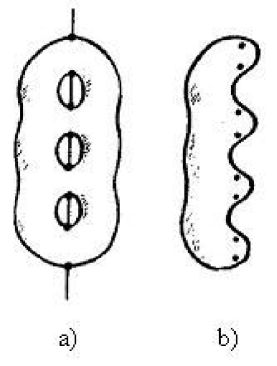
Figure 13: Riemann surface of genus g a) is a two-fold branched covering of a two sphere b)

Thus, $S^{2}=\mathcal{R}_{g}/i$, where ${i}$ is involution depicted in Fig.13. Let $Q_{g}=\{q_{1},...q_{2g+2}\}$ be the branching set of points on $S^{2}$ while $\tilde{Q}_{g}=\{\tilde{q}_{1},...\tilde{q}_{2g+2}\}$ the corresponding set of points on $\mathcal{R}_{g}$. From Birman, Ref.[77], page 182, one can find how the Dehn twists on $\mathcal{R}_{g}$ are related to the set $\tilde{Q}.$

In particular, to each Dehn twist on $\mathcal{R}_{g}$ one associates points $\tilde{q}_{2i-1}$ and $\tilde{q}_{2i}$ on $\mathcal{R}_{g}$  $(1\leq i\leq g)$ through which the $c_{i}$-th basis curve is passing. The Dehn twist on $\mathcal{R}_{g}$ is projected into $S^{2}$ in the form of the homeomorphism $\omega_{i}$ $(1\leq i\leq 2g+1)$ of $S^{2}$ resulting in exchange between the points $q_{2i-1}$ and $q_{2i}$ which leaves the rest of points fixed. If $\theta_{i}$ denotes the isotopy class of the Dehn twist about $c_{i}$, it can be demonstrated that such class obeys the braid group $\mathcal{B}_{n}$ relations given by $\theta_{i}\theta_{j}=\theta_{j}\theta_{i}$ if $\left|i-j\right|\geq 2$ and $\ \theta_{i}\theta_{i+1}\theta_{i}=\theta_{i+1}\theta_{i}\theta_{i+1}$ otherwise. In view of this, the mapping class group   of the $2g+2$ punctured sphere $\mathcal{M}_{S^{2}}(2g+2)$  is generated by a homomorphic image of these generators which can be represented by $2g+2$ strings (braids) generating the braid group. A presentation for $\mathcal{M}_{S^{2}}(2g+2)$  is given by the Theorem 4.5. of Birman’s book, Ref.[77]. Explicitly, it is given by

$$\begin{array}[]{c}\omega_{i}\omega_{j}=\omega_{j}\omega_{i}\text{ \ \ \ \ if }\left|i-j\right|\geq 2\text{ },\\ \omega_{i}\omega_{i+1}\omega_{i}=\omega_{i+1}\omega_{i}\omega_{i+1},\\ (\omega_{1},...,\omega_{2g+1})^{2g+2}=1,\\ \omega_{1}\cdot\cdot\cdot\omega_{2g}\omega_{2g+1}^{2}\cdot\cdot\cdot\omega_{1}=1.\end{array}$$ (7.1)

The  homomorphism just described sends $\theta_{i}$ to $\omega_{i}$. In view of the involution depicted in Fig.13, the kernel of this homomorphism is of order $2$. We are interested in finding out wether the Hecke algebra $H_{2g+1}$ can be associated with the presentation given by Eq.(7.1).

If $s_{i}$ is the generator for the symmetric group $S_{2g+1}$ (associated with exchange of  2 points on $S^{2})$ we are interested in mappings of   generators $T_{i}$ of Hecke algebra $H_{2g+1}$ into $s_{i}$ and $s_{i}$ into $\omega_{i}.$ This happens to be possible but nontrivial as discussed in the Jones paper, Ref.[76]. The nontriviality comes from the fact that representation $T_{i}^{\prime}s$ depends on $Q$ so that one has to satisfy the constraint $(\omega_{1},...,\omega_{2g+1})^{2g+2}=1$ for arbitrary $Q^{\prime}$s. Let $\pi_{Y}^{\prime}(s_{i})=\omega_{i}$ be the desired mapping (already from $T_{i}$ to $\omega_{i})$ with $Y$ indicating the Young tableaux associated with representation of the symmetric group. Lemma 9.2. by Jones allows us to make it in such a way that (irrespective to the actual value of $Q$) one obtains

$$\pi_{Y}^{\prime}(s_{1},...,s_{2g+1})^{2g+2}=1$$ (7.2a)

where the prime for $\pi_{Y}^{\prime}$ indicates  the needed ”adjustment” to make presentation Q-independent. Jones argues that the relation $\omega_{1}\cdot\cdot\cdot\omega_{2g}\omega_{2g+1}^{2}\cdot\cdot\cdot\omega_{1}=1$  in Eq.(7.1) is equivalent to $(\omega_{2},...,\omega_{2g+1})^{2g+1}=1.$ Accordingly, one obtains,

$$\pi_{Y}^{\prime}(s_{2},...,s_{2g+1})^{2g+1}=1.$$ (7.2b)

Based on this observation by Jones, one can continue this downsizing process thus obtaining the flag of Hecke algebras $\ H_{1}(Q)\subset H_{2}(Q)\subset\cdot\cdot\cdot H_{2g+1}(Q).$ The important theorem by Jones (to be used below) can be stated now as follows

Theorem 7.3.(Jones [76], page 361) Let Y be a Young diagram and let $\pi_{Y}^{\prime}$ be the corresponding representation of  $B_{2g+1}$ designed in such a way that Eq.(7.2a) holds (for any Q’s). Then $\pi_{Y}^{\prime}$ defines a representation of $M_{S^{2}}(2g+2)$ via $\omega_{i}\rightarrow\pi_{Y}^{\prime}(s_{i})$ if and only if Y is rectangular.

In other words, one begins with the rectangular Young tableaux of size $m\times n$ as discussed in Section 3 and obtains all Young tableaux which can fit into this rectangle by sequentially deleting boxes (one at the time).To finish this subsection we need to discuss difference between the mapping class group of the sphere $S^{2}$ and that of the disc $D^{2}.$  Since the disc can be viewed as a sphere with just one point deleted the generators $\omega_{i}$ described before can be used in the present case as well.  Thus we obtain the following theorem

Theorem 7.4. (Birman [77], page 32). Let M be a group of automorphisms of $\pi_{1}(D^{2}-Q_{n})$ which are induced by the homeomorphisms of $D^{2}-Q_{n}$ which keep the boundary of $D^{2}$ fixed poinwise. Then M is precisely the group $B_{n}.$

Remark 7.5. The fundamental group $\pi_{1}(D^{2}-Q_{n})$ is a free group of rank $n$. This group is made of loops anchored at some point in $D^{2}$ and such that each loop encloses only one puncture. In the next subsection this group will pay a role of monodromy group for the K-Z equation.

Remark 7.6. In the case of a sphere there is no boundary which is fixed pointwise. As result, one gets relations 3 and 4 in Eq.(7.1) which are simple consequences of rotational invariance of $S^{2}$ $($e.g. see Fig.13 of Ref.[77], page 157).

Being armed with these facts we are ready to discuss the next topic.

8.1 Monodromy  group of the Knizhnik-Zamolodchikov equations and the Riemann-Hilbert problem

The above discussion about the mapping class group seems to be detached from the rest of this paper. We would like to correct this deficiency now For this purpose, we need to remind to our readers about some basic facts from the theory of K-Z- type equations. According to Refs.[67,79] the K-Z Eq.(6.15) is equivalent to the following system of equations

$$\sum\limits_{i=1}^{n}\frac{\partial}{\partial z_{i}}f=0\text{ and }\kappa(\sum\limits_{i=1}^{n}z_{i}\frac{\partial}{\partial z_{i}})f=(\sum\limits_{i<j}\Omega_{ij})f.$$ (7.3)

The first of these equations comes from the fact that $\Omega_{ij}=\Omega_{ji}$. The second is obtained from Eq.(6.15) by multiplying both sides of this equation by $z_{i}$, summing over $i^{\prime}s$ and again taking into account that $\Omega_{ij}=\Omega_{ji}.$ The first of these equations indicates that solutions should be translationally invariant so that only differences of arguments must be used. The second implies that solutions must be homogenous. To extract this homogeneity we follow Ref.[69],page 37, and introduce new variables $\varsigma_{i}=\dfrac{z_{i+1}}{z_{i}}$, $i=1,...,n-1$, $\varsigma_{n}=z_{n}.$ In terms of these variables the K-Z equations acquire the following standard form

$$\varsigma_{i}\frac{\partial}{\partial\varsigma_{i}}f=A_{i}(\varsigma_{1},...,\varsigma_{n-1})f\text{ , }i=1,...,n,$$ (7.4)

where the $A_{i}^{\prime}s$ are holomorphic functions in the domain $D:=${$\left|\varsigma_{j}\right|<1,1\leq j\leq n\}.$ Such form of the K-Z equations allows us to use general local theory of linear differential equations of Fuchsian-type. In particular, the theorem  which is formulated and proved on page 121 of Ref.[80] provides the desired solution. It is given by

$$f=F_{0}(\varsigma_{1},...,\varsigma_{m})\varsigma_{1}^{A_{1}(0)}\cdot\cdot\cdot\varsigma_{m}^{A_{m}(0)},$$ (7.5)

where $F_{0}(\varsigma_{1},...,\varsigma_{m})$ is an $n\times n$ matrix- valued function holomorphic in the domain $\hat{D}:=\{\left|\varsigma_{j}\right|<1,1\leq j\leq m\}$ and such that $F_{0}(0)=Id.$These results allow us to mention about the Riemann-Hilbert (R-H) problem and by doing so to make a connection with previous subsection. The results which follow will bring us directly to the discussion of the G-W invariants.

To discuss the R-H problem in the domain $D$ we would like to rewrite Eq.s(7.4) in the following equivalent Fuchsian-type form [80]

$$\frac{\partial}{\partial\varsigma_{i}}f=\tilde{A}_{i}f,$$ (7.6)

where $\tilde{A}_{i}=A_{i}(\varsigma_{1},...,\varsigma_{n-1})/\varsigma_{i}.$ Consider now the limiting case: $\zeta_{i}\rightarrow 0$ for a subdomain $\bar{D}_{i}$ where presence of other singularities can be neglected. Without loss of generality we can subdivide $D$ into such subdomains so that the total (global) solution in $D$ is made of local solutions  in respective subdomains. The requirement that these solutions must agree in the overlapping regions is the essence of the R-H problem stated in simple terms. The $n=$ $2g+2$ punctured sphere discussed in the previous subsection can be looked upon as $2g+3$ punctured disc. Hence, we can initially develop our discussion for the disc $D$. In both cases: $D$ or $S^{2},$ the motion of subdomains $\bar{D}_{i}$  on these surfaces is controlled by the action of the respective braid groups as explained in the previous subsection.

Consider now a monodromy (holonomy) around given singularity. The existence of this monodromy is assured by the fact that Eq.(7.6) is linear equation whose solution is defined with accuracy up to a constant matrix which we shall call $T_{i}$. This matrix can be found by noticing that the matrix $\tilde{A}_{i}$ has only the first order (Fuchsian) pole as singularity. Going around this pole once  will pic up a phase resulting in the monodromy matrix $T_{i}$. It is given by $T_{i}=\exp(2\pi iA_{i}(0)).$ This can be easily understood with help of Eq.(7.5) taking into account the analytical properties of the logarithmic function. Consider now Eq.(7.5) in the overlap of two domains $\bar{D}_{i}$ and $\bar{D}_{j}.$ Evidently, in such domains we can use just one local coordinate so that at the overlap of these domains one has

$$F_{0}(\varsigma_{i})F_{0}^{-1}(\varsigma_{j})=\varsigma_{i}^{A_{i}(0)}\varsigma_{j}^{-A_{j}(0)}.$$ (7.7)

With help of Eq.(7.7) the R-H problem can be formulated now as a problem of finding  of a holomorphic vector function $\mathbf{f}(\varsigma)$ with good behavior at $\infty$  and such that in the complex plane C$\varsigma$ it obeys an equation $\mathbf{f}_{-}(\varsigma)=M(\varsigma)$ $\mathbf{f}_{+}(\varsigma)$ for some prescribed $n\times n$ matrix $M(\varsigma)$ and  for a contour (closed) $C$ in $\varsigma-$plane such that $\mathbf{f}_{+}(\varsigma)$ and $\mathbf{f}_{-}(\varsigma)$ lie respectively inside and outside of the domain enclosed by $C.$

This problem can be reformulated a bit differently as follows. Given a set of $n$ points $\{a_{1},...,a_{n}\}$ in $\mathbf{C}\varsigma$ and $n\times n$ matrices $A_{1},...,A_{n}$ representing the monodromy group $\mathcal{G}$ of these points find all equations of the type given by Eq.(7.6) which have the monodromy group $\mathcal{G}.$ We can complicate matters further by making the set of points to move in $\mathbf{C}\varsigma$ (or $S^{2}).$ This leads to the isomonodromic deformation problem. It can then be formulated as follows.

Problem 7.7. (Isomonodromy problem) For a given representation of the monodromy group $\mathcal{G}$ find dependence of matrices $\tilde{A}_{i}$ in Eq.(7.6) on location of poles given by the (moving) set $\{a_{1},...,a_{n}\}.$

This problem was solved by Schlesinger [81]. We would like to provide some needed details within the context of K-Z equations. In particular, taking into account that $\Omega_{ij}=\Omega_{ji}$ Eq.(6.15) can be rewritten as follows

$$df = \Gamma f,\text{ where}$$

$$\Gamma = \sum\limits_{1\leq i\leq j\leq n}\frac{\kappa^{-1}\Omega_{ij}}{z_{i}-z_{j}}(dz_{i}-dz_{j}).\TCItag{7.8}$$ (58)

The previously imposed requirement $[\mathcal{D}_{i},\mathcal{D}_{j}]=0$, e.g. see Eq.s(6.10),(6.11) can be now rewritten as $d(df-\Gamma f)=0$ implying the Frobenius- type equation $\Gamma\wedge\Gamma=0$ which holds only if

$$[\Omega_{ij},\Omega_{kl}]=0\text{ for }i\neq j\neq k\neq l$$ (7.9a)

and

$$[\Omega_{ij},\Omega_{ik}+\Omega_{jk}]=[\Omega_{ij}+\Omega_{ik},\Omega_{jk}].$$ (7.9b)

According to Kohno, Ref.[64], these are the infinitesimal pure braid relations. For $n=3$ they coincide with earlier obtained CYBE, Eq.s(6.11). Kohno, Ref.[64], demonstrated that, at least in the case of rational solutions of the CYBE’s, the results, Eq.s (7.9 a,b), can be brought into correspondence with the CYBE’s for $n>3$, i.e. for  $1\leq i\leq n.$ This result provides an independent support of earlier obtained Eq.(6.11) and connects us with the mapping class group presentation, Eq.(7.1). Evidently, the braid relations in Eq.(7.1) (adopted for $S^{2}$) become the YBE’s. Since the obtained isomorphism involves earlier discussed monodromy matrices we come to the conclusion that the monodromy representation for the K-Z equation is equivalent to the YBE representation. This is known as the Kohno-Drinfeld theorem,  Ref.[67], Thm 19.4.1. The introduced concepts even though being useful, play only an auxiliary role in this work. They were introduced mainly for the sake of the discussion presented in the next subsection.

8.2 The multiplicative Horn problem

8.2.1 Emergence of  Gromov-Witten invariants

In view of results we just obtained and, taking into account Eq.s(7.1), the monodromy matrices for the punctured sphere $S^{2}$ should be subjected to the following constraint

$$\prod\limits_{i=1}^{n}\exp(i2\pi A_{i})=\mathbf{I,}$$ (7.10)

where $\mathbf{I}$ is the unit matrix and $n=2g+1$.  Taking into account Remark 7.5., this equation has a simple geometrical meaning. It represents loops (holonomies or monodromies) around $n+1$ points, that is it represents the fundamental group $\pi$ of $S^{2}$ with points $\{a_{1},...,a_{n+1}\}$ deleted. As it is written, this equation suffers from the fact that it is not reflecting the differences between the topology of the disc D and that for the sphere S². Because of the Remark 7.5., this  equation cannot be used as such for the disc since the fundamental group $\pi_{1}(D^{2}-Q_{n})$ is free group of rank $n$. Even though it can be used for $S^{2}$ it does not reflect the constraint Eq.(7.2) adequately. Fortunately, this deficiency is easily correctable if we rewrite Eq.(7.10) in the alternative form  as follows

$$\prod\limits_{i=1}^{n}\exp(i2\pi A_{i})=\exp(i2\pi d\mathbf{I})$$ (7.11a)

with $d=0,1,2,..$. or, even more generally, as

$$\prod\limits_{i=1}^{n}\exp(i2\pi\frac{A_{i}}{d_{i}})=\exp(i2\pi\mathbf{I}).$$ (7.11b)

Matrices $\exp(i2\pi A_{i})$ are unitary by design and each of $A_{i}^{\prime}s$ is diagonalizable so that $\lambda(A_{i})=\{\lambda_{1}(A_{i}),...,\lambda_{k}(A_{i})\}$ represents the eigenvalue set for the matrix $A_{i}$. Since matrices $\exp(i2\pi A_{i})$ are unitary their determinant is 1. This leads to the requirement $\lambda_{1}(A_{i})+\cdot\cdot\cdot+\lambda_{k}(A_{i})=0(N\mathop{\mathrm{m}od}d_{i})$ $\forall i$ provided that $\sum\nolimits_{i}d_{i}=d.$ For the sake of comparison with earlier sections we would like to consider (without loss of generality) the case of $n=3$. Then, instead of Eq.(1.6), we obtain,

$$\lambda_{1}+\cdot\cdot\cdot\lambda_{k}+\mu_{1}+\cdot\cdot\cdot+\mu_{k}=\nu_{1}+\cdot\cdot\cdot+\nu_{k}+Nd_{1}+Nd_{2}+Nd_{3}$$ (7.12a)

which is essentially the K-M-B-B condition, Eq.(1.5). The same result can be rewritten as

$$\left|\lambda\right|+\left|\mu\right|=\left|\nu\right|+Nd.$$ (7.12b)

In view of this relation, the fusion rule, Eq.(3.7), should be modified accordingly. Following Ref.[$27$], we write

$$\sigma_{\lambda}\ast\sigma_{\mu}=\mathop{\textstyle\sum}\limits_{d,\nu}q^{d}C_{\lambda\mu}^{\nu}(d)\sigma_{\nu}.$$ (7.13)

The star symbol represents the product of ”quantum” cohomology classes. For $d=0$ this symbol becomes again the usual dot symbol  used in Eq.(3.7). The ”quantum”  L-R coefficients $C_{\lambda\mu}^{\nu}(d)$ are in fact the genus zero 3-point Gromov-Witten invariants which are structure  constants in the ”small” quantum cohomology ring [82].

The multiplication law, Eq.(7.13) takes place only if  Eq.(7.12b) holds. This equation replaces earlier equation $\left|\lambda\right|+\left|\mu\right|=\left|\nu\right|$ used for computations in Eq.(3.7). The r.h.s. of Eq.(7.13) is a polynomial in $q$ (where $q$ stays for ”quantum ”). Its physical role is clear from Eq.(7.13): it plays a role of fugacity associated with the degree of mapping $d$. More generally, in view of Eq.(7.11b), we should replace $q^{d}$ in Eq.(7.13) by $q^{d}=\mathop{\textstyle\prod}\limits_{i}q_{i}^{d_{i}}.$ To avoid unnecessary complications we shall be working just with $d$ from now on. Evidently, under such circumstances the $q$ indeterminate becomes an analog of $Q$ in the Hecke algebra, Eq.(6.9b), of the symmetric group. Connections with  the Hecke algebra are highly nontrivial. They are discussed  below and in Appendix C. In order to prepare our readers for this discussion we would like to proceed with actual computation of the G-W invariants.

There are many ways to compute these invariants. We would like to discuss only those which are logically compatible with results presented in previous sections.  In particular, we would like to connect the results presented in Section 5.3  with what has been discussed now. Following Walton, Ref.[83], we begin with the Weyl character formula, our (III.2.28). It is given by

$$\chi(\lambda)=\sum\limits_{w\in W}n_{w}(\lambda)e(w)$$ (7.14)

so that the fusion rule (Walton’s Eq.(1.5)) reads:

$$\chi(\lambda)\cdot\chi(\mu)=\sum\limits_{\nu\in\Delta_{+}}C_{\lambda\mu}^{\nu}\chi(\nu).$$ (7.15)

For the sake of space we refer to our Parts II (Appendix A) and Part III, Sections 1 and 2, for all definitions and notations. In Humphrey’s book, Ref. [84], on page 140 our readers can find (our) Eq.(7.15) with details of its derivation. Some of these details are discussed below. Clearly, since the constants $C_{\lambda\mu}^{\nu}$ will be different for different Weyl-Coxeter groups, the formulas above include the fusion rule, Eq.(3.8), as special case (for characters of symmetric group $S_{n}$ which  is of the type $A_{n-1\text{ }}$in Dynkin’s classification of the Weyl-Coxeter reflection groups). The Kostant multiplicity formula, Eq.(III.2.31), plays a very important role in Walton’s analysis. In particular, he uses it in order to arrive at the Steinberg’s formula for $C_{\lambda\mu}^{\nu}$

$$C_{\lambda\mu}^{\nu}=\sum\limits_{w,\mathfrak{v}\in W}\varepsilon(\mathfrak{v}w)P(w\lambda+\mathfrak{v}\mu-\nu).$$ (7.16)

In arriving at this result Eq.(III.2.31) for the Kostant multiplicity formula was used. Detailed derivation of the Steinberg’s formula can be found on page 141 of Ref.[84]. Explicit use of this formula is inconvenient though. It is given here to emphasize the combinatorial and symplectic nature of the L-R coefficients in accord with Section 5.3.. Since symplectic nature of $C_{\lambda\mu}^{\nu}$  was emphasized in Section 5.3., we brought  Eq.(7.16) to the attention of our readers  with additional purposes in mind. Specifically, Eq.(7.16) can be used not only for computations involving more traditional Weyl-Coxeter reflection groups but also for their affine extensions (e.g. see Appendix A for Part II for definitions). In this case Eq.(7.16) formally stays the same, except now the Weyl group $W$ is replaced by the affine Weyl group $W^{(k)}$ (or $W^{(m)})$ where $k$ (or $m$) have the same meaning as in our Eq.(3.3) (or (3.4)). This fact is not self-obvious and will be explained. Before doing so we note the following. Using Eq.(III.2.16) we know that $\varepsilon(\mathfrak{v}w)=(-1)^{l(\mathfrak{v}w)}=(-1)^{l(\mathfrak{v})}(-1)^{l(w)}.$ This observation allows us to rewrite the affine version of Eq.(7.16)  in equivalent form given by

$$C_{\lambda\mu}^{\nu(k)}=\sum\limits_{w\in W^{(k)}}\varepsilon(w)C_{\lambda\mu}^{w\cdot v}$$ (7.17)

with $C_{\lambda\mu}^{w\cdot v}$ representing standard L-R coefficient which can be calculated with help of honeycombs and puzzles as previously discussed. The fact that this is the case, unfortunately, is not sufficient for the efficient calculation of $C_{\lambda\mu}^{\nu(k)}.$ Hence, the task lies in finding the efficient scheme for such calculations. By doing so connections between the coefficients $C_{\lambda\mu}^{\nu(k)}$ and $C_{\lambda\mu}^{\nu}(d)$ will become apparent.

We begin with few definitions. In particular, in connection with the Young diagram defined by partition $\lambda,$ we define an $n$ rim- hook of this partition. It is a connected subset of $n$ boxes of $\lambda$ such that it does not contain a $2\times 2$ square. A rim-hook is legal if by removing it from the Young diagram $\lambda$ the remainder is still  be a valid Young diagram. Othervise, the $n$ rim- hook is considered to be illegal as depicted in Fig. 14.

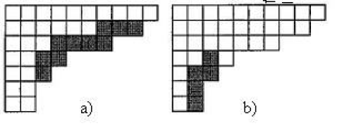
Figure 14: Legal a) and illegal b) rim hooks

An n-core for the partition $\lambda$ corresponds to a partition obtained by sequential removal of legal $n$-rim hooks till one obtains the configuration for which such removals are no longer possible. Let $\left|\lambda\right|$ be the weight of partition $\lambda,$ i.e. $\left|\lambda\right|=\lambda_{1}+\lambda_{2}+\cdot\cdot\cdot.$ Let then the weight of the resulting core partition be $\left|core_{n}\lambda\right|.$  The number $r_{n}(\lambda)$ =$\left(\left|\lambda\right|-\left|core_{n}\lambda\right|\right)/n$ is the number of $n-$ rim hooks removed in this process. Furthermore, define the width$\mathit{(R}_{i})$ of an $i$-th $n$-rim hook $R_{i}$ as the number of columns it occupies in the Young diagram. Let w_i=width$(R_{i})$ denote this number. As in Section 3.1, we place our original Young diagram into $m\times k$ rectangle so that $m+k=N$. Because of this, we write $C_{\lambda\mu}^{\nu}(d)=C_{\lambda\mu}^{\nu}(d;m,k)$ so that if, say, $\check{\lambda}$ is the partition conjugate to $\lambda,$ one can show  [86] that

$$C_{\lambda\mu}^{\nu}(d;m,k)=C_{\check{\lambda}\check{\mu}}^{\check{\nu}}(d;k,m)$$ (7.18)

in accord with the fact that $C_{\lambda\mu}^{\nu}=C_{\check{\lambda}\check{\mu}}^{\check{\nu}}$ for the ordinary L-R coefficients. To make actual computations using these definitions we need to use the following

Lemma 7.8. (Bertram, Ciocan-Fontanine, Fulton [86], page 733). If $\mu$ is the partition resulting from removing an n-rim hook from $\lambda$, then the (quantum) cohomology class $\sigma_{\lambda\text{ }}$is related to the (classical) cohomology class $\sigma_{\mu\text{ }}$ through the following relation

$$\sigma_{\lambda\text{ }}=(-1)^{k-w}q\sigma_{\mu\text{ }}$$ (7.19a)

where $w$ is the width of the n-rim hook and $k$ is the width of the Young tableaux containing partition $\lambda.$If $\lambda$ contains an illegal n-rim hook or if $\lambda_{m+1}>0$ and $\lambda$ contains no n-rim hooks or if $\lambda_{1}>k,$ then $\sigma_{\lambda\text{ }}=0.$

The above lemma allows us to use previously discussed fusion rule, Eq.(3.7), for calculation of the Gromov-Witten coefficients. We would like to show step-by -step how this is done. Let both partitions $\lambda$ and $\mu$ belong to the $m\times k$ rectangle and $R_{1},...,R_{r_{n}(\lambda)}$ be the respective $n-$rim hooks removed, then, instead of Eq.(7.19a), we obtain:

$$\sigma_{\lambda\text{ }}=\varepsilon(\lambda/\mu)q^{r_{n}(\lambda)}\sigma_{\mu\text{ }},$$ (7.19b)

where $\varepsilon(\lambda/\mu)=\prod\limits_{i=1}^{r_{n}(\lambda)}(-1)^{k-w_{i}}.$ If the partition $\mu$ is not contained in $m\times k$ rectangle, then $\sigma_{\mu\text{ }}=0.$ Next, we combine the fusion rule, Eq.(3.7), with just obtained result in order to obtain the prescription for calculation of the G-W invariants. Appendix B contains an example of calculation of G-W invariants in which the KT honeycombs are used for calculations of $C_{\lambda\mu}^{\nu}$ as an input. In actual  illustrative calculations done in Appendix B  we took into account that $d\equiv r_{N}(\lambda)$ and $n\rightarrow N$ in accord with Eq.(7.12b). Thus, in general, we obtain:

$$\sigma_{\lambda}\ast\sigma_{\mu}=\mathop{\textstyle\sum}\limits_{\nu\in k\times m}\mathop{\textstyle\sum}\limits_{d=0}q^{d}C_{\lambda\mu}^{\nu}(d;m,k)\sigma_{\nu}\text{,\ where }C_{\lambda\mu}^{\nu}(d;m,k)=\mathop{\textstyle\sum}\limits_{\rho}\varepsilon(\rho/\nu)C_{\lambda\mu}^{\rho}.$$ (7.20)

This result admits a somewhat different interpretation. For instance, let us introduce the ”quantum” cohomology class $\sigma_{\rho\text{ }}$ via

$$\sigma_{\rho\text{ }}=\mathop{\textstyle\sum}\limits_{d=0}q^{d}\mathop{\textstyle\sum}\limits_{\nu\in k\times m}\varepsilon(\rho/\nu)\sigma_{\nu},$$ (7.21)

then we can formally rewrite Eq.(7.20) as

$$\sigma_{\lambda}\ast\sigma_{\mu}=\mathop{\textstyle\sum}\limits_{\rho}C_{\lambda\mu}^{\rho}\sigma_{\rho\text{ }},$$ (7.22)

where $C_{\lambda\mu}^{\rho}$ is the classical L-R coefficient computable with help of KT honeycombs, puzzles or hives. This result is only in formal agreement with earlier obtained Eq.(3.7) since in Eq.(3.7) there is no restrictions on summation over $\rho$ while in the present case $C_{\lambda\mu}^{\rho}=$ $C_{\lambda\mu}^{\rho}(m,k)$ and is zero otherwise. Significance of such a restriction is discussed in the Appendix C. Obtained result is easy to understand using physical arguments. Indeed, using Eq.(7.12b) we notice that with $N\rightarrow\infty$ the only way to satisfy this equation is to let $d=0$. Hence, in view of the Theorem 5.1. Eq.(7.22) makes sense. Clearly, it  should be understood only as qualitative result since summation over $\rho$ is actually restricted.

We  have accumulated enough results enabling us to inject more physics into what was obtained thus far. This is done in the next subsection.

8.2.2 Verlinde algebra and Hecke algebra at the root of unity

While the mathematical meaning of G-W invariants, especially for small quantum cohomology ring, is discussed in many places, e.g. see Refs.[82,87,88], to our knowledge, this literature does not contain any information about physical significance of these invariants. We would like to correct this deficiency. By doing so we also will be able to sketch some missing links between these topics and those discussed in previous sections. We hope that our readers will use this material along with that of Appendix C as a point of departure for much deeper and thorough study.

We begin with observation that there are two ways to define the L-R coefficients: one is through the composition (fusion) law, Eq.(3.8), while the other through the Fourier series-type expansion of the skew Schur function $s_{\lambda/\mu}$ [37]. Specifically,

$$s_{\lambda/\mu}=\mathop{\textstyle\sum}\limits_{\nu}C_{\mu\nu}^{\lambda}s_{\nu}.$$ (7.23)

In view of Eq.(7.22) it is only natural to anticipate that there must be a ”quantum” analog of Eq.(7.23). Such an analog was indeed recently found by Postnikov [27]. We would like to connect his results with those in Ref.[86] using some results from the paper by McNamara [89].This will allow us to inject some physics into our discussion.

Recall that if $\lambda$ and $\mu$ are two partitions such that $\mu\subseteq\lambda$ if $\mu_{i}\leq\lambda_{i}$ $\forall i,$ then a pair $(\mu,\lambda)$ is called skew partition. For such a partition the Young diagram is made of diagram for $\lambda$ with $\mu$ removed. Traditionally used notation for such obtained diagram is given by $\lambda/\mu=(\lambda_{1},...,\lambda_{k})/(\mu_{1},...,\mu_{l}).$ Postnikov replaced the $m\times k$ rectangle used in calculations in Appendix B by the torus obtained from this rectangle by identification of its boundaries in a usual way. He considered skew partitions on such a torus and proved that Eq.(7.23), when adapted to this toroidal topology produces $C_{\lambda\mu}^{\nu}(d;m,k)$ as required. His derivation of this result  makes  the meaning of parameter $d$ especially transparent and suitable for potential physical applications (to be discussed below).

Remark 7.9. In view of Eq.s (7.11), (7.12) replacement of the rectangle by torus is completely natural. Moreover, in view of the fact that   in the most general case $q^{d}=\mathop{\textstyle\prod}\limits_{i}q_{i}^{d_{i}}$, it is surprising that instead of using the multidimensional torus the two dimensional torus is sufficient for reproduction of the G-W invariants. This peculiarity is explained below and in the Appendix C.

Following McNamara [89], for illustrative purposes we choose the basic rectangle $\boldsymbol{R}$ with parameters $k=3$ and $m=4.$The $\mu$ partition is chosen to be $\mu=(2,1)$ and the original $\lambda$ partition is chosen to be $\lambda=(4,4,4,4,2,1,1).$ Using the French style of writing of the Young tableaux (that is from the bottom-up) the skew tableaux $\lambda/\mu$ is depicted in Fig.15a).  Multiple copies of the same skew tableaux are depicted in the universal cover of the torus made of the basic rectangle in Fig.15b).  To recognize them in such setting one should pay attention to the vertical lines denoted as $V$ and the horizontal line denoted as $H$. The lower left corner of the original rectangle $\boldsymbol{R}$ coincides with the intersection of $H$ and $V$ lines. After that, the partition $\mu=(2,1)$ to be removed is easily recognizable. The boxes labeled by $x$ help us to identify the multiple copies of $\boldsymbol{R}$  so that the partition $\lambda$ can be readily identified

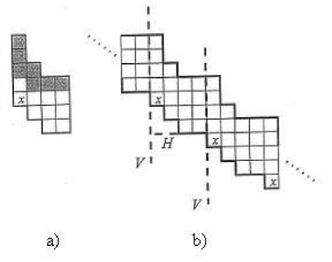
Figure 15: The skew tableaux a) and its torus equivalent b)

Next, we remove a shaded boxes from $\lambda$ which is equivalent of removal of one 7-rim hook (since in this example $k+m=7$). This leaves us with the partition $\lambda^{\prime}=(4,4,4,1).$ As it follows from the Fig.15, such a partition still does not fit the $\boldsymbol{R}$ so that we have to remove yet another 7-rim hook (just like in the Appendix B but in reverse). The resulting (core) partition $\lambda^{\prime\prime}=(3,3)$ does fit the rectangle $\boldsymbol{R}$.  Such obtained skew partition can be encoded by (3,3)/2/(2,1) or, more generally, $\lambda/d/\mu=(\lambda_{1},...,\lambda_{k})/d/(\mu_{1},...,\mu_{l}).$ Hence, $d=2.$

With such defined  toric skew partitions one can replace Eq.(7.23) by

$$s_{\lambda/d/\mu}=\mathop{\textstyle\sum}\limits_{\nu\in k\times m}C_{\mu\nu}^{\lambda}(d;m,k)s_{\nu}.$$ (7.24)

If in the $d-$sum in Eq.(7.20) only one term is nonzero, then $C_{\mu\nu}^{\lambda}(d;m,k)$ in Eq.(7.24) is the desired G-W invariant. In Ref.[90], page 379, Witten argued that  for dimensional reasons in the $d-$sum in Eq.(7.20) only one term should be nonzero. If this is the case, then $C_{\mu\nu}^{\lambda}(d;m,k)$ in Eq.(7.24) is the G-W invariant  and coincides with that given in Eq.(7.20). Moreover, if in Eq.(7.20)  we formally choose $q=1$ thus obtained fusion rule coincides exactly with that for the Hecke algebra, Eq.(6.9b), for which $Q$ is the $m$-th root of 1, i.e. $Q^{m}=1($recall that $N=m+k)$ as it was demonstrated by Goodman and Wenzl [91]. These authors noticed that under such circumstances the fusion coefficients coincide with those for the Verlinde algebra for $su(k)$ Wess-Zumino-Witten  (WZW) CFT model at the level $m$.

Remark.7.10. Since connections with representations of Hecke algebra are insured by previous stated Theorem 7.3. by Jones, while connections between the K-Z type equations and theWZW-type models were established by Knizhnik and Zamolodchikov [92], this explains (in view of Goodman-Wenzl results) why in calculations of G-W invariants presented above and in Appendix B the rectangular boxes are used.

Remark 7.11.  These facts are not sufficient for explanation of the mathematical meaning of the rim-hook removals (additions) in such calculations. This deficiency is corrected to a some extent in Appendix C.

Obtained results give us an opportunity to discuss some additional physical applications.

8.2.3 Possible applications to solid state physics

In Part I, Eq.(I,3.22), or in Eq.(1.5) of this work, we noticed that such an equation can be interpreted within a context of solid state physics. In view of earlier obtained results we would like to discuss this connection in some detail now. In solid state physics the Bloch theorem [5] reflects the difference between the wave function in the vacuum and that in the periodic solid. Account for periodicity requires the wave function to be written in the form $\Psi_{\mathbf{k}}(\mathbf{r})=e^{i\mathbf{k\cdot r}}u_{\mathbf{k}}(\mathbf{r}),$ where $u_{\mathbf{k}}(\mathbf{r})$ is some periodic function. The vector $\mathbf{k}$ is determined by the condition

$$e^{i\mathbf{k\cdot l}}=1,$$ (7.25)

where $\mathbf{l}$ is the minimal translation vector of the direct lattice. Since this type of equation we have encountered already in Part II, e.g. see Eq.(II.9.18), we know that solution is given by

$$\mathbf{k\cdot l=0\mathop{\mathrm{m}od}}\text{ }2\pi d$$ (7.26)

which implies that the vector $\mathbf{k}$  should belong to the reciprocal (or dual) lattice and $d$ should be some integer.  In Part I we called this equation as the Kac-Moody-Bloch-Bragg condition (K-M-B-B condition). Clearly, Eq.(7.11) is of the same type. This fact underscores its solid state physics relevance. In particular, it causes all physically interesting quantities to change accordingly so that, for instance, the momentum vectors for electrons are defined only with accuracy  up to some vectors of the reciprocal lattice. This causes energy of the electron not to be well defined (as explained below). Eq.(7.26) suggests strong links with number theory. The book by Terras, Ref.[93], especially Chr.10, provides an excellent starting point for development of theory of electronic band structures of solids (and also of molecules) using methods of number theory. Clearly, in doing so one has to use group theory in the number fields of characteristic other than zero as explained in Appendix C.

Some uses of the WZW-type models in solid state physics are mentioned in the book by Tsvelik [94]. Thus far they are restricted only to 1+1 dimensional models whose exact solutions can be obtained by other methods anyway. We would like to argue that all many -body problems of solid state physics in which lattice periodicity cannot be disregarded should employ mathematical formalism discussed in this paper.

That this is the case can be seen from the simplest example. Indeed, the existing band theory of solids [5] is essentially the theory one electron in the periodic 3d lattices, e.g. all known lattices  $\mathcal{L}$ are made as direct sum  $\mathcal{L}$=$\left(\boldsymbol{Z}/m_{1}\mathbf{Z}\right)\oplus\left(\boldsymbol{Z}/m_{2}\mathbf{Z}\right)\otimes\left(\boldsymbol{Z}/m_{3}\mathbf{Z}\right),$  where $m_{1},m_{2},m_{3}$ are respective lattice periods. All such lattices have 2 kinds of symmetry: point-like and spatial. The affine Weyl-Coxeter reflection groups are capable of describing these symmetries. The word ”affine” accounts for effects of translational symmetry of the lattice (as explained in Appendix A to Part II). This symmetry is so important that the presence of potential in the Schrödinger equation can be often ignored [95]. The band theory developed for the ”empty” lattice sometimes is sufficient for good reproduction of experimental data. For the empty lattice the energy $\mathcal{E}(\mathbf{k})$ of a single electron is known to be [96], Chr1.,

$$\mathcal{E}(\mathbf{k})=\frac{\hbar}{2m}\left|\mathbf{k}+\mathbf{K}\right|^{2},$$ (7.27)

where $\mathbf{K}$ is any vector of the reciprocal lattice.  In view of Eq.(7.25) the vector $\mathbf{k}$ can have only finite number of values [96]. Unlike the traditional band theory of solids dealing with one electron in periodic lattice $\mathcal{L,}$ we would like to place several electrons into such a lattice so that the total energy of noninteracting (except, due to the Pauli principle) is given by

$$\frac{2m}{\hbar}E^{T}=\mathop{\textstyle\sum}\limits_{i}\left|\mathbf{k}_{i}+\mathbf{K}\right|^{2}.$$ (7.28)

Since the vector $\mathbf{K}$ is arbitrary we choose it to be the same for all electrons. If this is the case, the above expression can be rewritten as

$$\frac{2m}{\hbar}E^{T}=\mathop{\textstyle\sum}\limits_{i}(\mathbf{k}_{i}^{2}+2\mathbf{k}_{i}\mathbf{\cdot K+K}^{2}).$$ (7.29)

Since the total momentum of such system of electrons should be conserved this requires us to write

$$\mathop{\textstyle\sum}\limits_{i}\mathbf{k}_{i}=0.$$ (7.30)

Finally, summing over all energy levels (whose number is finite), that is taking a trace of the corresponding matrix operator, brings us back to the equation analogous to Eq.(7.12a). The Pauli exclusion principle requires the total wave function to be antisymmetric. This requirement is satisfied by the factorized wave function made of product of spin and coordinate-dependent part. In the absence of lattice periodicity the procedure of constructing such antisymmetric total wave function for several electrons can be found in the book by Messiah, Ref.[97]. This procedure uses essentially the representation theory of symmetric group $S_{n}$. Presence of lattice periodicity replaces $S_{n}$ by its affine analog as discussed in Appendix C. The above picture can be complicated by accounting for effects of the constant magnetic field acting on electrons in periodic lattices. Rigorous mathematical treatment of this problem has been initiated in works by Novikov and his collaborators [98]. The small quantum cohomology ring discussed in earlier subsections becomes the Novikov ring under present circumstances [82].

Acknowledgement The author would like to thank Allen Knutson (U of California, Berkeley) for his kind permission to reproduce some figures from his papers (with T.Tao and C.Woodward) in this paper.

Appendix A. Details of Heisenberg’s derivation of the commutator identity $[\hat{x},\hat{p}]=i\hbar$

In this Appendix we would like to provide some details of Heisenberg’s reasoning leading to the discovery of $[\hat{x},\hat{p}]=i\hbar$.  We do this for several reasons. First, this would be unnecessary should his original Nobel Prize winning paper, Ref. [18], contain all details and would be free of typographical errors. Second, although in Section 5 we mentioned Dirac’s acknowledgement (on page 177 of his book, Ref.[22]) of the fact that light scattering experiments associated with measurement of the refractive index (or dielectric constant) and their theoretical interpretation had lead Heisenberg to his discovery of quantum mechanics, nowhere in the existing literature  on quantum mechanics were we able to find exposition using this historic fact as the starting point for  the development of quantum mechanical formalism.

At the classical level consider a gas of noninteracting atoms, better just one atom containing $N$ electrons which are assumed to scatter light independently. The interaction between the incoming light and such an electron is described with help of the combination d$=\beta$E where d is the dipole moment of the electron in the atom, E is the strength of the external electric field which is assumed to be time-dependent, and $\beta$ is the polarization tensor (in the simplest case it is assumed to be a scalar). In the medium the strength of the electric field changes as compared to the vacuum. By denoting it as D it is known that D=E +4$\pi\mathbf{P}$ where P=Nd. Since, at the same time, by definition, d=er we have to have an equation for r. It is given by

$$\mathbf{\ddot{r}}+\omega_{0}^{2}\mathbf{r+\gamma\dot{r}=}\frac{e}{m}\mathbf{E(}t\mathbf{),}$$ (A.1)

where $e$ is electron’s charge and $m$ is its mass. In writing this equation it is assumed that our electron is bound harmonically (with the basic frequency $\omega_{0}^{2})$ and that the friction is of  known (electromagnetic) nature and is assumed to be small. Using Fourier decomposition of r(t) we obtain,

$$\mathbf{r}(\omega)=\frac{e}{m}\frac{\mathbf{E}}{\omega_{0}^{2}-\omega^{2}+i\omega\gamma}.$$ (A.2)

This equation allows us to obtain P and, hence, D as follows :

$$\mathbf{D}=\mathbf{E}+4\pi\mathbf{P}=(1+4\pi N\text{ }\frac{e^{2}}{m}\frac{1}{\omega_{0}^{2}-\omega^{2}+i\omega\gamma})\mathbf{E}\equiv\varepsilon(\omega)\mathbf{E.}$$ (A.3)

This equation defines a complex frequency-dependent dielectric constant $\varepsilon(\omega).$ From electrodynamics it can be equivalently rewritten as $\varepsilon(\omega)=(n(\omega)-i\varkappa(\omega))^{2}$ where $n(\omega)$ is the refractive index while $\varkappa(\omega)$ is the coefficient of absorption. Using these facts we can write approximately

$$n(\omega)=1+2\pi N\text{ }\frac{e^{2}}{m}\frac{1}{\omega_{0}^{2}-\omega^{2}+i\omega\gamma}.$$ (A.4)

By ignoring friction in the high frequency limit we obtain,

$$n(\omega)=1-2\pi N\text{ }\frac{e^{2}}{m\omega^{2}}.$$ (A.5.)

To account for quantum mechanical effects, Thomas, Reich and Kuhn in 1925 (just before the quantum mechanics was born !) have suggested to replace Eq.(A.4) by

$$n(\omega)=1+2\pi N\text{ }\frac{e^{2}}{m}\sum\limits_{i}\frac{f_{i}}{\omega_{i0}^{2}-\omega^{2}},$$ (A.6)

where, following these authors, we ignored friction and introduced the oscillator strength $f_{i}.$To reconcile Eq.(A.6) with (A.5) we have to require $\sum\limits_{i}f_{i}=1.$ This requirement is known as the sum rule.  These facts were known to Kramers and Heisenberg, Ref.[99], where our readers can find additional details. To make our point and to save space, we would like to reobtain the result, Eq.(A.6), quantum mechanically  using modern formalism. We refer our reader to Ref.[100], pages 316-319], for additional details. Basically, we need to calculate quantum mechanically the dipole moment d, that is

$$\mathbf{d}_{m}=\int\psi_{m}^{\ast}e\mathbf{r}\psi_{m}d^{3}\mathbf{r.}$$ (A.7.)

In this expression the wave function $\psi_{m}$ is calculated with help of the stationary perturbation theory with accuracy up to the first order in perturbation (which is er$\cdot$E). A short calculation produces the following result for the oscillator strength:

$$f_{km}=\frac{2m\omega_{km}}{\hbar}\left|\left\langle k\mid\hat{x}\mid m\right\rangle\right|^{2}.$$ (A.8)

This result can be equivalently rewritten as

$$f_{km}=\frac{m\omega_{km}}{\hbar}\{\left\langle k\mid\hat{x}\mid m\right\rangle^{\ast}\left\langle k\mid\hat{x}\mid m\right\rangle+\left\langle k\mid\hat{x}\mid m\right\rangle^{\ast}\left\langle k\mid\hat{x}\mid m\right\rangle\}.$$ (A.9)

Since, however,

$$im\omega_{km}\left\langle k\mid\hat{x}\mid m\right\rangle=\left\langle k\mid\hat{p}_{x}\mid m\right\rangle$$ (A.10)

we can rewrite Eq.(A.9) as

$$f_{km}=\frac{1}{i\hbar}\{\left\langle m\mid\hat{x}\mid k\right\rangle\left\langle k\mid\hat{p}_{x}\mid m\right\rangle-\left\langle m\mid\hat{p}_{x}\mid k\right\rangle\left\langle k\mid\hat{x}\mid m\right\rangle\}$$ (A.11)

since $\omega_{km}=-\omega_{mk}$. Finally, we have to require $\sum\limits_{k}f_{km}=1.$ This is possible only if

$$\frac{1}{i\hbar}\left\langle m\mid\hat{x}\hat{p}_{x}-p_{x}\hat{x}\mid m\right\rangle=1,$$ (A.12)

QED.

Appendix B. An example of detailed computation of $C_{\lambda\mu}^{\nu,d}(m,k).$

In this appendix we  would like to work out an example of computation of the Gromov-Witten invariant $C_{\lambda\mu}^{\nu,d}(m,k)$ based on Example 1 taken from Ref.[86]. Our calculations differ however from those in Ref.[86] since we use the KT scheme for computation of the classical L-R coefficients.

In Example 1 the basic Young tableaux rectangle is taken as $m\times k=5\times 5$. From here we obtain: $m+k=N=10$  Hence, the length of the rim-hooks to be used is 10. Next, we are given partitions $\lambda=(5,4,4,2,2),\mu=(3,2,1)$ and $\nu=(2,1).$ Based on these data, we can calculate the weights. These are respectively $\left|\lambda\right|=17,\left|\mu\right|=6$ and $\left|\nu\right|=3.$ Since we know already that $N=10,$ the fundamental relation, Eq.(7.11b), that is $\left|\lambda\right|+\left|\mu\right|=\left|\nu\right|+dN$ now leaves us no choice for $d$. We obtain, $d=2$. But this number gives us the number of the 10-rim hooks to be used in our computations, that is 2. If we choose $\nu$ as the core partition then, indeed, only 2 rim hooks will fill in the rectangle as depicted in Fig.16 below

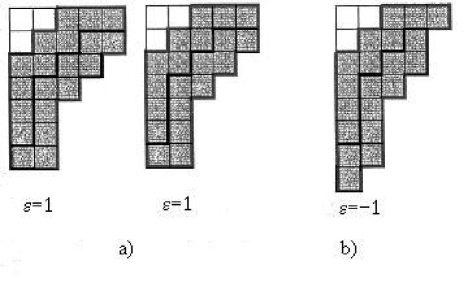
Figure 16: $\rho_{1}$ with its rim-hooks and phase factors a), the same for $\rho_{2}$ b)

The filling of the rectangle (in the present case- the square) is made in such a way that the added rim hooks must not be added beyond the pre assigned width of the rectangle but, at the same time, they are allowed to occupy more height space than the rectangle can provide. This results in two partitions $\rho_{1}=(5,5,4,3,2,2,2)$ and  $\rho_{2}=(5,4,4,3,2,2,2,1)$  which can be read off directly from Fig.16. The summation over $\rho$ in Eq.(7.20) in the present case takes place over $\rho_{1}$ and $\rho_{2}.$ The phase factor $\varepsilon(\rho/\nu)$ under this summation can be easily computed based on the information given in Fig.16. For this purpose we need to calculate the widths of the 10-rim hooks in both tableaux depicted in Fig.16. For the first tableaux the widths are $w_{1}=5$ and $w_{2}=5$ respectively. Hence, the overall phase factor $\varepsilon(\rho_{1}/\nu)=(-1)^{5-5}\cdot(-1)^{5-5}=1$. Analogously, for the second tableaux the phase factor $\varepsilon(\rho_{2}/\nu)=(-1)^{5-5}\cdot(-1)^{5-4}=-1.$To complete our calculation, we need the actual values for the classical L-R coefficients $C_{\mu\nu}^{\rho_{1}}$ and $C_{\mu\nu}^{\rho_{2}}.$ We calculate them graphically with help of the KT method using Fig.6 as an example. This example indicates that we have to make some adjustments in the initial data for partitions in order to be able to use the KT scheme.

Hence, let us begin with calculations of $C_{\mu\nu}^{\rho_{1}}$. The enlarged partitions having the same number of entries are $\lambda=(5,4,4,2,2,0,0),\mu=(3,2,1,0,0,0,0)$ and $\rho_{1}=(5,5,4,3,2,2,2)$. It should be noted that the locations of the added zeros are quite arbitrary and that their redundancy should be discarded in actual calculations (that is this redundancy should not affect the numerical value of $C_{\mu\nu}^{\rho_{1}}).$ With these remarks we need to make a set of Y-shaped tripods of the type depicted in Fig.1. By doing so we need to match together the numbers from $\lambda$ and $\mu$ partitions in such a way that the partition $\rho_{1}$ is obtained. Also, we must pay attention to the order  in which the labeling of the honeycomb is made, e.g. see Fig.3.  After that, the number of possibilities for such type of matching is $C_{\mu\nu}^{\rho_{1}}.$ If we disregard redundancy of added zeros, then we straightforwardly obtain $C_{\mu\nu}^{\rho_{1}}=2$ . To repeat this procedure for $\rho_{2}$ we need to use the following partitions $\lambda=(5,4,4,2,2,0,0,0),\mu=(3,2,1,0,0,0,0,0)$ and $\rho_{2}=(5,4,4,3,2,2,2,1).$ The result of matching now produces $C_{\mu\nu}^{\rho_{2}}=1$.Hence, altogether we obtain: $C_{\lambda\mu}^{\nu}(d;m,k)=2-1=1,$ in accord with Ref.[86].

Appendix C. Hecke algebra and Kashiwara crystals

The purpose of this Appendix is only to provide a list of key references needed in support of results of the main text. Obviously, the choice of references is subjective. Nevertheless, it  is hoped that it provides a sufficient background level needed for reading any other literature on these subjects.

We begin with Eq.(7.22). This result can be looked upon using theory of k-restricted (bounded) partitions recently developed by Lapointe and Morse [101]. These authors were looking at the following problem: how fusion, Eq.(3.8), is going to change if instead of standard Schur functions $s_{\lambda}$ one would use $k-$bounded Schur functions $s_{\lambda}^{(k)}$ indexed by partitions $\lambda$ whose first part (i.e. $\lambda_{1})$ is no larger than a fixed integer $k\geq 1?$ For such functions the L-R coefficient $C_{\lambda\mu}^{\nu}$ should be replaced by $C_{\lambda\mu}^{\nu,k}.$ These authors managed to prove (see their Theorem 18) that, in accord with our Eq.(7.22), for the appropriately chosen $\ k$  (actually for $k=N-1$) the coefficient $C_{\lambda\mu}^{\check{\nu},N-1}$ $=C_{\lambda\mu}^{\nu,d}(m,k)$ (with $N=k+m$). These results can be looked upon from broader perspective [102].To this purpose we introduce the affine symmetric group $\hat{S}_{k}$ generated by $k$ elements $\hat{s}_{0},\hat{s}_{1},,..,\hat{s}_{k-1}$ and satisfying the affine Coxeter relations

$$\begin{array}[]{c}\hat{s}_{i}^{2}=1,\\ \hat{s}_{i}\hat{s}_{j}=\hat{s}_{j}\hat{s}_{i}\text{ , }i-j=\pm\text{1}\mathop{\mathrm{m}od}k,\\ \hat{s}_{i}\hat{s}_{i+1}\hat{s}_{i}=\hat{s}_{i+1}\hat{s}_{i}\hat{s}_{i+1}.\end{array}$$ (C.1)

The generators $\hat{s}_{i}$ should be understood as $\hat{s}_{i\mathop{\mathrm{m}od}k}$ if $i>k.$The usual symmetric group $S_{k}$ embeds into $\hat{S}_{k}$ as a subgroup generated by $s_{0},s_{1},,..,s_{k-1}$ but this embedding is not unique: there are many embeddings among which one has to choose the most convenient [102]. The question arises: how $s_{\lambda}^{(k)}$ is connected with representations for $\ \hat{S}_{k}?$ We would like to give an answer in several steps. First, we recall that the Hecke algebra $H_{n}$ is the deformation of $S_{n}$ with the  deformation parameter $Q.$ Characters of symmetric group $s_{\lambda}$ and those for Hecke algebra have the same fusion algebra controlled by the L-R coefficients (as discussed in the main text), except for the case when Q is a nontrivial root of 1. In the last case the fusion algebra for the Hecke characters coincides with the Verlinde algebra as demonstrated by Goodman and Wenzl [91]. Lapointe and Morse [101] argue that the fusion algebra for $k-$bounded Schur functions $s_{\lambda}^{(k)}$ coincides with the Verlinde algebra for the WZW models.  Since generators $D_{i}$ in Eq.(6.9) for the Hecke algebra $H_{n}$ are deformations of the generators $s_{i}$ for symmetric group $S_{n},$ one can think about deformation of generators $\hat{s}_{i}$ for the affine symmetric group $\hat{S}_{n}.$ In Ref.[103] one can find that such a deformation is described by the affine Hecke algebra $\hat{H}_{n}(Q)$ which is the Weyl reflection group for the affine Lie algebra $\begin{array}[]{c}\widehat{\mathbf{sl}}_{n}.\end{array}$ Finally, according to Ref.s[104], [105] representations of $\widehat{\mathbf{sl}}_{n}$ and those for the Hecke algebra at root of unity are interrelated albeit  in a very nontrivial way (as explained below). Hence, $s_{\lambda}^{(k)}$ (up to a constant) may coincide with representation for the Hecke algebra at $\sqrt[n]{1}.$ $s_{\lambda}^{(k)}$ form a Schubert basis for the cohomology ring of the affine Grassmannian as it is explained by Lam [106]. Affine Grassmannian was recently discussed in works by Kapustin and Witten [107] and also, independently, by Frenkel [108]. In both cases it was discussed in connection with applications of  methods of number theory to string and CFT.

Because of this, we would like to explain how the number theory enters into previous discussion. For this purpose, we would like to discuss the notion of a crystal and a crystal base following Ref.[109]. A crystal is made of a set $B$ endowed with the maps $\tilde{e}_{i},\tilde{f}_{i}:B\sqcup\{0\}\rightarrow B\sqcup\{0\}$ ($i\in I),$ where $I$ is an index set. These maps satisfy the following conditions: a) $\tilde{e}_{i}0=\tilde{f}_{i}0=0;b)$ $\tilde{e}_{i}^{n}b=\tilde{f}_{i}^{n}b=0$ $\forall b\in B$ and $i\in I$ , c) $\exists b,b^{\prime}\in B$ and$\ i\in I$ such that $b^{\prime}=\tilde{f}_{i}b$ if and only if $b=\tilde{e}_{i}b^{\prime}.$

The above definition is too abstract to see the connection with crystals. This deficiency is easily correctable. Using results and notations of Appendix A (Part II) we introduce the weight lattice $P_{l}^{+}$ (typical for the affine reflection groups) by

$$P_{l}^{+}=\{\mathop{\textstyle\sum}\limits_{i=0}^{n}a_{i}\omega_{i}\mid a_{i}\geq 0,\text{ }a_{i}\in\mathbf{Z}\text{ }\forall i=1\div n;\mathop{\textstyle\sum}\limits_{i=0}^{n}a_{i}=l\}$$ (C.2)

so that $B=P^{+}=\mathop{\textstyle\bigcup}\nolimits_{l>0}P_{l}^{+}.$ At the same time, Eq.(C.2) has the number-theoretic meaning (e.g.see Ref.[110], Appendix) in the case if $a_{i}\in\mathbf{F}_{q}\equiv\mathbf{Z}/q\mathbf{Z}$ with $q$ being some prime number. In this case the expansion $\beta=$ $\mathop{\textstyle\sum}\limits_{i=0}^{n}a_{i}\omega_{i}$ can be interpreted as an expansion of a number $\beta$ which belongs to the field extension of the number field $\mathbf{F}_{q}.$ Since such an extension corresponds to a particular solution of the familiar (by now) equation $\mathop{\textstyle\sum}\limits_{i=0}^{n}a_{i}=l,$ different solutions of this equation represent different numbers $\beta$. This observation is sufficient for explanation of a role of the operators $\tilde{e}_{i}$ and $\tilde{f}_{i}$ in the emerging picture.  Indeed, by analogy with Section 3 we can associate with each solution of $\mathop{\textstyle\sum}\limits_{i=0}^{n}a_{i}=l$ the Young diagram. The new element in doing so lies in the fact that boxes in such Young tableaux should be filled with numbers which belong to the field $\mathbf{F}_{q}$. This is rather easy to do, e.g. see Ref.[105]. With this information, a crystal graph can be constructed as follows. We take a set of $\beta^{\prime}s$ as vertices of the graph (so that $\beta^{\prime}s\rightleftharpoons b^{\prime}s)$ then, the operators $\tilde{f}_{i}$ connect vertices related by $b^{\prime}=\tilde{f}_{i}b.$ The index $i$ represents a color so that the crystal graph is directed and colored by colors from the set $I$. The connections with representation theory and fusion can be figured out now based on the observation that different $\beta^{\prime}s$ are in one-to one correspondence with different Young diagrams. Each such diagram encodes a character for the respective group, e.g. in characteristic zero characters for $S_{n}$ are the Schur functions $s_{\lambda},$etc.Hence, as we just explained, the crystal graphs can be used instead of KT honeycombs (or puzzles) for calculation of fusion coefficients [111].

Finally, we would like to provide a few additional details regarding the actual role being played by the operators $\tilde{f}_{i}$ and $\tilde{e}_{i}$ in order to connect the results of this appendix to that of Appendix B and Section 7.4.2. In these sections we’ve noticed that different Young diagrams can be obtained from the set of core Young diagrams by adding(removing) the appropriate rim-hooks. The core Young diagrams can be looked upon as representing a vacuum state while the addition(removal) of the particular rim-hook is done by the raising (lowering) operator. In the simplest case we are dealing with addition(removal) of just one box of the Young diagram. Hence, we can associate the addition (removal) of just one box with the operator $\tilde{e}_{i}$ (with the operator $\tilde{f}_{i}).$ Clearly, if we need to remove(add) a rim-hook the appropriate combination of such raising (lowering) operators should be used. Interestingly enough, a systematic development of the formalism we just sketched leads to the Heisenberg commutation rule, Eq.(5.8). Details can be found in Ref.[112]. The same formalism for $q=1$ is used for description of representations of the Hecke algebra H${}_{m}(\sqrt[n]{1})$, Ref.[105], page 279.

Remark. We would like to mention that the concept of a crystal was developed by Kashiwara, e.g. see Ref.[113], in connection with obtaining the exact solution of XXZ model in the thermodynamic limit (that is in the limit of infinite spin chain). The same authors notice that the whole formalism of quantum groups, vertex operators, Virasoro algebra, etc. was developed and makes sense either for infinite chains or for finite chains with appropriately chosen boundary conditions. In the case of finite chains without specially chosen boundary conditions the whole apparatus of this Appendix fails. This observation is very important for development of our new string- theoretic formalism. It is totally consistent with results presented in Parts I-III and will be further discussed in Part IV, especially in connection to and comparison with recent alternative string-theoretic developments[114].

References

[1] A.Kholodenko, New strings for old Veneziano amplitudes I.

Analytical treatment,  J.Geom.Phys.55 (2005) 50-74.

[2] A.Kholodenko, New strings for old Veneziano amplitudes II.

Group-theoretic treatment, J.Geom.Phys.56 (2006) 1387-1432.

[3] A.Kholodenko, New strings for old Veneziano amplitudes III.

Symplectic treatment, J.Geom.Phys.56 (2006) 1433-1472.

[4] R.Stanley, Combinatorics and Commutative Algebra,

Birkhäuser, Boston, 1996.

[5] J.Ziman, Principles of the Theory of Solids,

Cambridge University Press, Cambridge, UK, 1972.

[6] S.Ghorpade,G.Lachaud, Hyperplane sections of Grassmannians

and the number of MDS linear codes,

Finite fields  Their Appl. 7 (2001) 468-506.

[7] V. Kac, Infinite Dimensional Lie Algebrs,

Cambridge University Press, Cambridge, UK, 1990.

[8] N.Bourbaki, Groupes at Algebres de Lie

(Chapitre 4-6), Hermann, Paris,1968.

[9] R.Stanley, Enumerative Combinatorics, Vol.I,

Cambridge University Press, Cambridge, UK, 1999.

[10] H.Weyl, Das asymptotische Verteiilungsgesetz der

Eigenwerte lineare partieller Differentialgleichungen,

Math.Ann. 71 (1912) 441-479.

[11] S.Daftuar, P. Hayden, Quantum state transformations and the

Schubert calculus, Ann. Physics 315 (2005) 80–122.

[12] A.Klyachko, Quantum marginal problem and representation

of the symmetric group, arxiv.org : quant-ph/0409113.

[13] A.Horn, Eigenvalues of sums of Hermitian matrices,

Pacific J.of Math. 12 (1962) 225-241.

[14] A. Klyachko, Stable vector bundles and Hermitian operators,

Selecta Math.(N.S.) 4 (1998) 419-445.

[15] A.Knutson,T.Tao, The honeycomb model of GL_n(C) tensor

producsts I: Proof of the saturation conjecture,

J.AMS 12 (1999) 1055-1090.

[16] A.Knutson,T.Tao, C.Woodward, The honeycomb model of GL_n(C)

tensor producsts II: Puzzles determine facets of the

Littlewood-Richardson cone, J.AMS 17 (2003) 19-48.

[17] S.Friedland, Finite and infinite dimensional generalizations of Klyachko’s

theorem, Linear Algebra Appl. 319 (2000) 3–22.

[18] W.Heisenberg, Collected Works, pages 382-396,

Springer-Verlag, Berlin, 1985.

[19] A.Kholodenko, New strings for old Veneziano amplitudes IV.

Connections with spin chains and

other stochastic systems, arXiv:0805.0113.

[20] A.Knutson, T.Tao, Honeycombs and sums of Hermitian matrices,

AMS Notices 48 (2001) 175-186.

[21] P.Dirac, Fundamental equations of quantum mechanics,

Proc.Roy.Soc.(Lond) A109 (1925) 642-653.

[22] P.Dirac, Principles of Quantum Mechanics,

Clarendon Press, Oxford, 1930.

[23] B.Lidskii, Spectral polytope for the sum of two Hermitian matrices,

Funct.Analysis Applic. (in Russian) 16 (1982) 76-77.

[24] A.Zelevinsky, Littlewood-Richardson semigroups. Math. Sci. Res. Inst.

Publ., 38, Cambridge Univ. Press, Cambridge, 1999.

[25] S.Mandelstam, Dual resonance models, Phys.Reports13 (1974) 259-353.

[26] R.Bott, L.Tu, Differential Forms in Algebraic Topology,

Springer-Verlag, Berlin, 1982.

[27] A.Postnikov, Affine approach to quantum Schubert calculus,

Duke Math.J. 128 (2005) 473-509.

[28] H.Hiller, Geometry of Coxeter Groups,

Pitman Advanced Publ.Program, Boston, 1982.

[29] W.Fulton, Young Tableaux, Cambridge U.Press,

Cambridge, 1997.

[30] L.Manivel, Symmetric Functions, Schubert Polynomials

and Degeneracy Loci, Soc. Math.de France, Paris, 1998.

[31] H.Tamvakis, The connection between representation theory

and Schubert calculus, Enseign. Math. 50 (2004) 267–286.

[32] I.Macdonald, Symmetric Functions and Orthogonal Polynomials,

AMS University Lecture Notes Vol.12, Providence, RI, 1998.

[33]  L.Lapointe, L.Vinet, Exact operator solution of the

Calogero-Sutherland model, Comm. Math. Phys. 178 (1996) 425–452.

[34]  J.Minahan, A. Polychronakos, Equivalence of two-dimensional QCD

and the c=1 matrix model, Phys. Lett. B 312 (1993) 155–165.

[35]  A. Gorsky, N. Nekrasov, Relativistic Calogero-Moser model

as gauged WZW theory. Nuclear Phys. B 436 (1995) 582–608.

[36]  I.Macdonald, Symmetric Functions and Hall Polynomials,

Clarendon Press, Oxford, 1995.

[37]  R.Stanley, Enumerative Combinatorics, Vol.II,

Cambridge University Press, Cambridge, UK, 1999.

[38]  W.Fulton, Eigenvalues, invariant factors, highest weights,

and Schubert calculus, Bull. Amer. Math. Soc.

(N.S.) 37 (2000) 209–249.

[39]  W.Dittrich, M.Reuter, Classical and Quantum Dynamics,

Springer-Verlag, Berlin, 1992.

[40]  V.Arnol’d, Mathematical Methods of Classical Mechanics,(in Russian)

Moscow, Nauka, 1974.

[41]  M.van Leeuwen, The Littlewood-Richardson rule and related

combinatorics, MSJ Memoirs 12 (2001) 95-145.

[42]  A.Berenstein, A. Zelevinsky, Tensor product multiplicities and

convex polytopes  in partition space. J. Geom. Phys. 5 (1988) 453–472.

[43]  R.King, C. Tollu, F. Toumazet, Stretched Littlewood-Richardson

and Kostka coefficients, CRM Proc. Lecture Notes, 34 (2004) 99–112,

AMS, Providence, RI, 2004.

[44]  A.Buch, The saturation conjecture (after A.Knutson and T.Tao,

with appendix by Fulton ), Enseign.Math.46(2000) 43-60.

[45]  I.Pak, E.Vallejo, Combinatorics and geometry of

Littlewood-Richardson cones,

European J. of Combinatorics, 26 (2005) 995-1008.

[46]  H.Derksen, J.Weyman, On the Littlewood-Richardson polynomials,

J.of Algebra 255 (2002) 247-297.

[47]  A.Kholodenko, Kontsevich-Witten model from 2+1 gravity:

new exact combinatorial solution, J. Geom.Physics 43 (2002) 45-91.

[48]  M.Born, Mechanics of Atom, (In German),

Springer-Verlag, Berlin, 1924.

[49]  W.Pauli, M.Born, Über die Quantelung gest örther mechanischer

Systeme, Z.Phys.10 (1922) 137-158.

[50]  E.Baly, Spectroscopy, Longmans,Green and Co, London, 1905.

[51]  M.Born, W.Heisenberg, P. Jordan, Zür Quantenmechanick II,

Z.Phys. 35 (1926) 557-615.

[52]  S.Adler, Quantum Theory as Emergent Phenomenon,

Cambridge University Press, Cambridge, 2004.

[53]  P.Orlik, H. Terao, Arrangements and Hypergeometric Integrals,

MSJ Memoirs, Vol.9, Tokyo, 2001.

[54]  K.Aomoto, Configurations and invariant Gauss-Manin connections

of integrals. I. Tokyo J. Math. 5 (1982) 249–287.

[55]  V.Vassiliev, Applied Picard-Lefschetz Theory, AMS,

Providence, RI, 2002.

[56]  M.Saito, B.Sturmfels, N.Takayama, Gröbner Deformations of

Hypergeometric Differential Equations, Springer-Verlag, Berlin, 2000.

[57]  E. Opdam, Multivariable hypergeometric functions,

European Congress of Mathematics, Vol. I (Barcelona, 2000), 491–508,

Progr. Math., 201, Birkhäuser, Basel, 2001.

[58]  A.Kirillov Jr., Lectures on affine Hecke algebras and Macdonald’s

conjectures, Bull. Amer. Math. Soc. (N.S.) 34 (1997) 251–292.

[59]  M.Rösler, M.Voit, Markov processes related with Dunkl operators,

Adv.Appl.Math. 21 (1998) 575-643.

[60]   J-M.Soriau, Structure of Dynamical Systems,

Birkhäuser, Boston, 1997.

[61]   S.Bates, A.Weinstein, Lectures on Geometry of Quantization,

AMS, Providence, RI,1997.

[62]   P.Diaconis, Group Representations in Probability and Statistics,

Inst.of Math.Statistics Lecture Notes, Vol.11, Hayward, Ca,1988.

[63]   A. Lascoux, M-P Schützenberger, Symmetry and flag manifolds,

LNM 996 (1980) 118-144.

[64]   T.Kohno, Linear representations of braid groups and classical

Yang-Baxter equations, Cont.Math. 78 (1988) 339-363.

[65]   M.Atiyah, The Geometry and Phyics of Knots,

Cambridge University Press, Cambridge, 1990.

[66]   C.K.Fan, Structure of a Hecke algebra quotient,

J.AMS 10 (1997) 139-167.

[67]   K.Kassel, Quantum Groups, Springer-Verlag, Berlin, 1995.

[68]   A.Belavin, V.Drinfel’d, Solutions of classical Yang-Baxter

equation and simple Lie algebras,  Funct.Anal.Appl.

16 (1982) 159-180.

[69]   P.Etingof, I.Frenkel, A.Kirillov Jr., Lectures on Representation

Theory and Knizhnik-Zamolodchikov Equations,

AMS, Providence, RI, 1998.

[70]   O.Gleizer, A. Postnikov, Littlewood-Richardson coefficients

via Yang-Baxter equation,

Internat. Math. Res. Notices  14 (2000) 741–774.

[71]    H.Wenzl, Hecke algebras of type $A_{n}$ and subfactors,

Inv.Math.92 (1988)349-383.

[72]     M.Jimbo, A q-analogue of $U(\mathfrak{g}l(N+1))$ Hecke algebra, and the

Yang-Baxter equation, Lett. Math. Phys. 11 (1986) 247–252.

[73]      A.Ram, A Frobenius formula for the characters of the Hecke algebras,

Invent. Math. 106 (1991) 461–488.

[74]     A.Lascoux, B. Leclerc, J-Y.Thibon, Flag varieties and the

Yang-Baxter equation, Lett. Math. Phys. 40 (1997) 75–90.

[75]     R.King,  B. Wybourne, Representations and traces of the Hecke

algebras $H_{n}(q)$ of type $A_{n-1},$ J. Math. Phys. 33 (1992) 4–14.

[76]     V. Jones, Hecke algebra representations of braid groups and link

polynomials, Ann.Math.126 (1987) 335-388.

[77]    J.Birman, Braids, Links , and Mapping Class Groups,

Princeton University Press, Princeton, 1975.

[78]     A.Kholodenko, Use of quadratic differentials for description of

defects and textures in liquid crystals and 2+1 gravity,

J. Geom. Phys. 33 (2000) 59–102.

[79]     B.Bakalov, A.Kirillov Jr., Lectures on Tensor Categories and

Modular Functors, AMS, Providence, RI, 2001.

[80]     D.Anosov, S.Aranson, V.Arnol’d, I.Bronshtein,V.Grines,

Yu.Ilyashenko, Ordinary Differential equations and Smooth

Dynamical Systems, Springer-Verlag, Berlin, 1997.

[81]     M.Ablowitz, P.Clarkson, Solitons, Nonlinear Evolution

Equations and Inverse Scattering,

Cambridge University Press, Cambridge, 1991.

[82]     D.McDuff, D.Salamon, J-Holomorphic Curves and

Symplectic Topology, AMS, Providence, RI, 2004.

[83]     M.Walton, Tensor products and fusion rules,

Canadian J.of Physics 72 (1994) 727-736.

[84]     J.Humphreys, Introduction to Lie Algebras and Representation

Theory, Springer-Verlag, Berlin, 1972.

[85]      V.Guillemin, E.Rassart, Signature quantization and representations

of compact Lie groups, Proc. Natl. Acad. Sci.

USA 101 (2004) 10884–10889.

[86]       A.Bertram, I. Ciocan-Fontanine, W. Fulton, Quantum multiplication

of Schur polynomials. J. Algebra 219 (1999) 728–746.

[87]      D.Cox, S. Katz, Mirror Symmetry and Algebraic Geometry,

Mathematical Surveys and Monographs, Vol. 68,

AMS, Providence, RI, 1999.

[88]     W.Fulton, R. Pandharipande, Notes on stable maps and quantum

cohomology, Proc. Sympos. Pure Math. Vol 62 (1995) 45-96.

[89]        P.McNamara, Cylindric skew Schur functions, arxiv: math.CO/0410301.

[90]      E.Witten, The Verlinde algebra and the cohomology

of the Grassmannian, in Geometry, Topology and Physics

for Raoul Bott, pp357-422., International Press Inc., Boston, 1995.

[91]      F.Goodman, H. Wenzl, Littlewood-Richardson coefficients for Hecke

algebras at roots of unity, Adv. Math. 82 (1990) 244–265.

[92]      V.Knizhnik, A. Zamolodchikov, Current algebra and Wess-Zumino

model in two dimensions, Nuclear Phys. B 247 (1984) 83–103.

[93]     A.Terras, Fourier Analysis on Finite Groups and Applications,

Cambridge University Press, Cambridge, 1999.

[94]     A.Tsvelik, Quantum Field Theory in Condensed Matter Physics,

Second edition, Cambridge University Press, Cambridge, 2003.

[95]     F.Herman, Theoretical investigation of the electronic energy band

structure of solids, rev.Mod.Phys. 30 (1958) 102-121.

[96]     J.Callaway, Energy Band Theory, Academic Press, New York, 1964.

[97]    A.Messiah, Quantum Mechanics, Vol.2, North Holland,

Amsterdam, 1962.

[98]     S.Novikov, A.Maltsev, Topological phenomena in normal metals,

arxiv: cond-mat/9709007.

[99]      H.Kramers, W.Heisenberg, On the dispersion of radiation by atoms

(In German), Z.fur.Phys.31 (1925) 681-708.

[100]      A.Davydov, Quantum Mechanics, Pergamon, Oxford, 1965.

[101]      L.Lapointe, J.Morse, Quantum cohomology and the k-Schur basis,

arxiv: math.CO/0501529.

[102]        T.Lam, Affine Stanley symmetric functions, arxiv:math.CO/0501335.

[103]      M. Kashiwara, T. Miwa, E.Stern, Decomposition of q-deformed

Fock spaces, arxiv: math.q-alg/9508006.

[104]      A.Lascoux, B.Leclerc, J-Y.Thibon, Hecke algebras at rooths of

unity and crystal bases of quantum affine algebras,

Comm.Math.Phys. 181 (1996) 205-263.

[105]     O.Foda, B.Leclerc, M.Okado, J-Y.Thibon, T.Welsch,

Combinatorics of solvable lattice models and modular

representation of Hecke algebras, in Geometric Analysis

and Lie Theory in Mathematical Physics, pp. 243-290,

Cambridge University Press, Cambridge, 1998.

[106]     T.Lam, Schubert polynomials and affine Grassmannian,

arxiv: math.CO/0603125.

[107]      A.Kapustin, E.Witten, Electric-magnetic duality and Langlands

program, arxiv: hep-th/0604151.

[108]      E.Frenkel, Lectures on the Langlands program and conformal

field theory, arxiv: hep-th/0512172.

[109]      S.Kang, M.Kashiwara, K.Misra,T.Miwa, T.Nakashima,

A.Nakayashiki, Perfect crystals of quantum affine Lie algebras,

Duke Math. Journal 68 (1992) 499-608.

[110]      A.Kholodenko, ”New” Veneziano amplitudes from ”Old” Fermat

(hyper) surfaces, in

Trends in Mathematical Physics Research, pp1-94,

Nova Science Publishers, New York, 2004.

[111]      G.Fourier, P.Littlemann, Weyl modules, Demazure modules,

K-R modules, crystals, fusion products and limit constructions,

arxiv: math.RT/0509276.

[112]      T.Lam, Ribbon tableaux and the Heisenberg algebra,

Math. Z. 250 (2005) 685–710.

[113]      B.Davies, O.Foda, M.Jimbo, T.Miwa, A.Nakayashiki,

Diagonalization of the XXZ Hamiltonian by vertex operators,

arxiv: hep-th/9204064.

[114]      A.Gorsky, Gauge theories as string theories: the first results,

Physics Uspekhi 175 (2005) 1145-1162.