hep-th/0608xxx
FIT HE - 06-02

Shear viscosity of Yang-Mills theory

in the confinement phase

Iver Brevik and Kazuo Ghoroku

^∗ Department of Energy and Process Engineering, Norwegian University of Science and Technology, N-7491 Trondheim, Norway
^†Fukuoka Institute of Technology, Wajiro, Higashi-ku
Fukuoka 811-0295, Japan

In terms of a simple holographic model, we study the absorption cross section and the shear viscosity of a pure Yang-Mills field at low temperature where the system is in the confinement phase. Then we expect that the glueball states are the dominant modes in this phase. In our holographic model an infrared cutoff $r_{m}$ is introduced as a parameter which fixes the lowest mass of the glueball. As a result the critical temperature of gluon confinement is estimated to be $T_{c}\sim 127$ MeV. For $T<T_{c}$, we find that both the absorption cross section and the shear viscosity are independent of the temperature. Their values are frozen at the values corresponding to the critical point, for $0<T<T_{c}$. We discuss this behavior by considering the glueball mass and its temperature dependence.

1 Introduction

Recently, Policastro, Son and Starinets [1] have given a nice application of holographic calculations for the shear viscosity. This viscosity could be observed in the hot QGP phase of QCD. The calculation is based on the gravity/gauge correspondence [2, 3, 4, 5], and assumes a strongly coupled 4d YM theory.

With regard to experiments the situation is however unfortunate, since the quark-gluon plasma one hopes to create in heavy-ion experiments has relatively low temperature at which the coupling constant is strong and the perturbation theory in QCD works poorly. So we expect that an approach in terms of holographic models, utilizing the gravity/gauge correspondence, would be very useful for the understanding of the various experimental result in this region.

Recently, we have found that the holographic model available at high temperature can be extended also to the low temperature quark confinement phase by introducing an infrared cutoff [6, 7]. This approximate model could give successful results for the thermal properties, masses of light mesons, decay constants etc, in the low temperature confinement phase of 4d YM theory. In the confinement phase, the physical states of QCD would be hadrons. Then we would be able to see the thermodynamical properties of the hadron gas by applying our approximate model to the 4d YM theory in the low temperature phase.

In the present paper we study the shear viscosity, which is related to the absorption cross section of gravitons [1]. We first study the absorption cross section of gravitons falling perpendicularly onto D3-branes in the confinement phase. The calculation is performed in a way similar to that of Refs. [8, 9]. Then we extend the calculation to the finite temperature case in order to see the temperature dependence of the shear viscosity of hadron gas, i.e. the glueball gas in the present case.

2 Absorption by deformed D3 Brane

The shear viscosity is related to the absorption cross section, so we firstly study this quantity at zero temperature to understand the situation in the confinement phase.

The D3-brane metric can be written as

$$ds^{2}=H^{-1/2}\left(-dt^{2}+dx_{1}^{2}+dx_{2}^{2}+dx_{3}^{2}\right)+H^{1/2}\left(dr^{2}+r^{2}d\Omega_{5}^{2}\right),$$

where

$$H=1+{R^{4}\over r^{4}}\ .$$

The s-wave of a minimally coupled massless scalar satisfies

$$\left[\rho^{-5}{d\over d\rho}\rho^{5}{d\over d\rho}+1+{(\omega R)^{4}\over\rho^{4}}\right]\phi(\rho)=0\ ,$$ (1)

where $\rho=\omega r$. For small $\omega R$ the absorption cross section was obtained by Klebanov [8] by solving the matching problem of an approximate solution in the inner region and the outer region. The following result was obtained,

$$\sigma_{\rm 3-brane}={\pi^{4}\over 8}\omega^{3}R^{8}\ .$$ (2)

And this is also precisely given from 4d $\cal{N}$=4 SYM theory as a three point vertex of the bulk field and the fields of SYM theory which are given by the Born-Infeld action.

In this case, the 4d $\cal{N}$=4 SYM theory is described by string theory or by supergravity near the horizon of the D3-branes. In this limit, the geometry is approximated by Ad$S_{5}\times S^{5}$ and the equation of motion for the dilaton ($\phi$) or for the graviton polarized parallel to the D3 brane is written as

$$\left(\partial_{r}^{2}+{5\over r}\partial_{r}+M_{g}^{2}[1+(R/r)^{4}]\right)\phi=0,$$ (3)

where $M_{g}$ denotes the 4d mass of the dilaton. However, for Ad$S_{5}\times S^{5}$, there is no finite $M_{g}$ which gives a normalizable wave function $\phi$ since $\cal{N}$=4 SYM is not a confining theory. To obtain a confining YM theory, the bulk geometry should be deformed to an appropriate form. In this case, however, the geometry has a complicated form especially in the infrared region.

A simple and tractable approximation for such a confining geometry can be given by introducing an infrared cutoff at an appropriate point of the coordinate $r$, say $r=r_{m}$. In this case, the geometry Ad$S_{5}\times S^{5}$ is used in the region $r_{m}<r<\infty$. This approximation would be justified since the main deformation of the geometry is in the infrared region, $r<r_{m}$, and this region is cut off now. In fact, we can obtain a discrete mass spectrum for the glueball by solving (3) and imposing the boundary condition $\partial_{r}\phi|_{r_{m}}=0$. When we adopt the lattice result for the glueball mass, $M_{g}\sim 1.5$ GeV, the IR cutoff is set at $r_{m}\sim 0.4$ in units where $R=1$. Here we used the data in [10] since the temperature dependence of the glueball mass is given in this reference. We see that it is consistent with our analysis given in Fig.1.

Now we turn to the absorption cross section for the deformed D3 branes, whose horizon limit background is given by the Ad$S_{5}\times S^{5}$ with IR cutoff. Then the background, which describes also off the horizon limit, can be written as (2) with the IR cutoff $r_{m}$. So the matching problem is solved in a similar way as that developed by Klebanov. The only difference is the existence of the IR cutoff, and the equation is restricted to the region $r_{m}<r<\infty$. We call the region near $r_{m}$ the inner region.

While the wave equation is solved in terms of Bessel functions at small $\rho$ [8], we here solve the equation at some small but finite $r$, namely at the IR cutoff $r_{m}(<R)$. To study the wave function in this region, Eq.(1) is solved by rewriting it according to [9] as

$$\left[\partial_{\tau}^{2}+\omega_{m}^{2}\right]\phi(\tau)=0\ ,\quad\tau=-{1\over 4\rho^{4}}\ ,$$ (4)

$$\omega_{m}=\rho_{m}^{5}\sqrt{1+(\omega R)^{4}/\rho_{m}^{4}},\quad\rho_{m}=\omega r_{m}$$

The solution of this form of equation can be matched to the outer solution. Then, near $r_{m}$, the incoming wave is given as

$$\phi(\tau)_{\rm~{}in}=e^{-i\omega_{m}\tau}$$ (5)

and this is approximated for small $\tau$ as

$$\phi(\tau)_{\rm~{}in}=1-i\omega_{m}\tau\,$$ (6)

In the outer region, (1) is estimated by substituting $\phi=\rho^{-5/2}\psi$. Then we get

$$[{d^{2}\over d\rho^{2}}-{15\over 4\rho^{2}}+1+{(\omega R)^{4}\over\rho^{4}}]\psi=0\ .$$ (7)

Now the last term is negligible for $\rho\gg(\omega R)^{2}$, where (7) is solved in terms of Bessel functions as

$$\phi_{\rm out}=A\rho^{-2}\left[J_{2}(\rho)+biN_{2}(\rho)\right]\ ,$$ (8)

$J$ and $N$ being the Bessel and Neumann functions.

From the matching of the solutions, (5) and (8), in the overlapping region of $r$, we obtain $A=1$ and $b=0$. Then

$$\phi_{\rm out}={1\over 8}\rho^{-2}J_{2}(\rho)\,.$$ (9)

In terms of the formula for the invariant flux $F$,

$$F={1\over 2i}\sqrt{-g}~{}g^{~{}rr}(\phi^{*}\partial_{r}\phi-c.c.),$$ (10)

the fluxes of the incoming wave are obtained as

$$F_{\rm inner}=\omega g_{m},$$ (11)

$$g_{m}=r_{m}^{5}\sqrt{1+(R/r_{m})^{4}}$$

near $r_{m}$, and

$$F_{\rm outer}={32\over\pi}\omega^{-4}.$$ (12)

for the outer region. Then the absorption probability at $r_{m}$ is given as

$${\cal{P}}=|{F_{\rm inner}\over F_{\rm outer}}|={\pi\over 32}\omega^{5}g_{m}\,.$$ (13)

We notice that the power of $\omega$ is different from the case of D3 background without the IR cutoff.

The absorption cross-section $\sigma$ is related to the s-wave absorption probability by [9]

$$\sigma={(2\pi)^{5}\over\omega^{5}\Omega_{5}}{\cal P}\ ,$$

where

$$\Omega_{D}={2\pi^{{D+1\over 2}}\over\Gamma\left({D+1\over 2}\right)}$$

is the volume of a unit $D$-dimensional sphere. Thus, for the 3-brane we find the following cross section at the infrared cutoff $r_{m}$,

$$\sigma_{\rm IR}={\pi^{3}g_{m}}\ .$$ (14)

We notice that this result is independent of $\omega$ contrary to the case of the background without the cutoff, and it is proportional to the area of the five dimensional sphere with radius $r_{m}$. So the situation is similar to the absorption by a black body in the six dimensional space.

In the case of background without the cutoff, the cross section is explained by the decay amplitude of the incoming scalar to two gluons or other fields included in the SYM theory [8, 11, 12]. In this case, the semiclassical calculation is useful because of the conformal invariance of the YM theory. And the gluons are not bounded to glueballs in spite of the interactions with a strong coupling constant. In the present case, however, the conformal invariance of the gauge theory is of course lost and the gluons are confined and bounded to glueball states. Then we expect that the incoming scalar of energy $\omega$, which is in the range $M_{g}<\omega<2M_{g}$, will form a glueball after it coupled to the gluon pair. For $\omega>2M_{g}$, there appears the possibility of pair production of glueballs, and it would be possible to calculate the pair production cross section as in the YM case. But the interaction between the glueballs is complicated and strong. It would be difficult to get some useful results from the 4d field theory side. This point will be discussed more in the future.

3 Extension to finite temperature

For the finite temperature gauge theory, the corresponding gravity background solution is given by the nonextremal black three-brane. It has the form [13, 14]

$$ds^{2} = H^{-1/2}(r)[-f(r)dt^{2}+d{\vec{x}}~{}^{2}]$$ (15)

$$+H^{1/2}(r)[f^{-1}(r)dr^{2}+r^{2}d\Omega_{5}^{2}]\,,$$

where as before $H(r)=1+R^{4}/r^{4}$ and $f(r)=1-r_{0}^{4}/r^{4}$. The Hawking temperature of this metric is

$$T={r_{0}\over\pi R^{2}}\ ,$$ (16)

and the metric of the previous section is obtained for $T=0$. It is well known that gravity under this background in the near-horizon limit of D3 branes describes the high temperature deconfinement phase of the YM theory. On the other hand, we have proposed that the low temperature confinement phase could be obtained by introducing the IR cutoff, $r_{m}$, in this holographic model as $r_{0}<r_{m}(<R)$ [6, 7]. When the two phases are separated at $r_{0}=r_{m}$, the critical temperature $T_{c}$ is given as

$$T_{c}={r_{m}\over\pi R^{2}}\sim 127~{}{\rm MeV}\ .$$ (17)

Next we consider the $s$-wave radial equation for a minimally coupled scalar (such as the graviton polarized parallel to the brane), $\partial_{\mu}(\sqrt{-g}g^{\mu\nu}\partial_{\nu}\phi)=0$. For the metric (15) this equation acquires the form

$$\partial_{\rho}(\rho^{5}f\partial_{\rho}\phi)+{H\rho^{5}\over f}\phi=0\ .$$ (18)

We solve this equation in two phases, one at low and one at high temperature, and give the absorption cross sections in each phase.

3.1 Low temperature phase $T<T_{c}$

By introducing the IR cutoff $r_{0}<r_{m}(<R)$, the low temperature phase is obtained for the range of $r_{m}<r<\infty$ in terms of the metric (15). Here, we consider $r_{m}$ to be independent of the temperature or of $r_{0}$. We estimate the absorption cross section at the IR cutoff as in the previous section. Near $r=r_{m}$, Eq.(18) is rewritten as

$$\left[\partial_{\tilde{\tau}}^{2}+{\omega}_{m}^{2}\right]\phi(\tilde{\tau})=0\ ,$$ (19)

$$\quad{\partial\tilde{\tau}\over\partial r}={1\over\rho^{5}f}\ ,$$ (20)

where we notice ${\omega}_{m}=\rho_{m}^{5}\sqrt{1+(\omega R)^{4}/\rho_{m}^{4}},\quad\rho_{m}=\omega r_{m}.$ Then at the IR cutoff, the incoming wave is given as

$$\phi(\tilde{\tau})_{\rm~{}in}=e^{-i{\omega}_{m}\tilde{\tau}},$$ (21)

and this is approximated for small $\tilde{\tau}$ as

$$\phi(\tilde{\tau})_{\rm~{}in}=1-i{\omega}_{m}\tilde{\tau}.\,$$ (22)

On the other hand, in the region of large $\rho$, we can approximate $H\sim 1$ and $f\sim 1$, then we arrive at the same form of solution as in the previous section,

$$\phi=\tilde{A}\rho^{-2}\left[J_{2}(\rho)+\tilde{b}iN_{2}(\rho)\right]\ .$$

As in the previous section, the outer solution is given as

$$\phi_{\rm out}={1\over 8}\rho^{-2}J_{2}(\rho)\,,$$

and this matches with (21) at an appropriate region near $r_{m}$. Then we arrive at the same result for the fluxes of the incoming wave as that obtained for $T=0$,

$$F_{\rm inner}=\omega g_{m},$$ (23)

where $g_{m}=r_{m}^{5}\sqrt{1+(R/r_{m})^{4}}$ as shown above. We should notice here that the factor $f(\rho)$ has disappeared in the final result of (23) due to the exact cancellation between the wave function and the measure in (10). As a result, $F_{\rm inner}$ is independent of the temperature.

Now, $F_{\rm outer}$ is the same as given in (12) at zero temperature. Then all other quantities are the same as in the zero temperature case. The absorption probability at $r_{m}$ is given as

$${\cal{P}}=|{F_{\rm inner}\over F_{\rm outer}}|={\pi\over 32}\omega^{5}g_{m}\,,$$ (24)

and we obtain the absorption cross section at low temperature,

$$\sigma_{\rm 3-brane}^{\rm lowT}={\pi^{3}g_{m}}\,.$$ (25)

This result is seen to be independent of the temperature and it has the same form as that obtained at zero temperature. This point can be understood as follows. Since $T<T_{c}<<M_{g}$, the thermal fluctuations of glueballs would be suppressed because we need large energy, at least $\omega>M_{g}$, to obtain a definite thermal effect, which should in principle be expressed by some kind of temperature dependence, according to a thermal field theory for the glueball gas.

In the above discussion we neglected the temperature dependence of the glueball mass $M_{g}(T)$, but it will be important. It is estimated here by solving the equation of motion of the dilaton near the D3 horizon limit of (15).

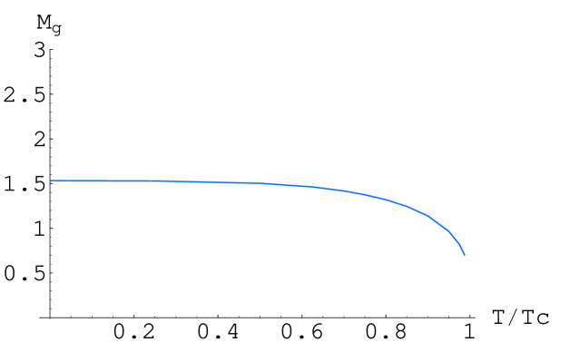
Fig. 1: Glueball mass vs temperature, for $r_{m}=0.4$ and $R=1$.

The equation to be solved is

$$\left(\partial_{r}^{2}+\partial_{r}\left(\log(r^{5}f(r))\right)\partial_{r}+M_{g}^{2}{1+(R/r)^{4}\over f^{2}}\right)\phi=0,$$ (26)

and the mass eigenvalue $M_{g}$ is obtained by finding the normalizable solutions of this equation. The numerical results are given in Fig.1 for $r_{m}=0.4$ and $R=1$. We observe its typical $T$-dependence, $M_{g}\to 0$ for $T\to T_{c}$, and this behavior can be understood by the last term in the equation. The similar behaviour has been seen also in [6, 7] and it is consistent with the lattice analysis [10] as pointed out above. From these results we can say that the above $T$-independence of (25) would be modified near $T_{c}$ since $M_{g}$ becomes small at this point and the probability of pair production of glueballs can not be neglected in this region.

It is obvious that the temperature dependence of the mass comes from the factor $f$ in the equation. On the other hand, the factor $f$ is absent in (25). Therefore, the temperature dependence has to be included in the parameter $r_{m}$ itself, when $\sigma_{\rm 3-brane}$ is temperature dependent. In other words, $r_{m}$ will vary with temperature, at least near $T=T_{c}$. This point will be discussed in the next sub-section.

3.2 High temperature phase

At high temperature, $r_{m}<r_{0}$, we consider the region of $r_{0}<r<\infty$ where we can see the deconfinement phase of the gauge theory. Here we estimate the absorption at the horizon $r_{0}$. Near $r=r_{0}$, Eq. (18) has the form

$$\phi^{\prime\prime}+{\phi^{\prime}\over r-r_{0}}+\left({\omega\over 4\pi T}\right)^{2}{\phi\over(r-r_{0})^{2}}=0\,.$$ (27)

The matching problem has been solved as in [1], and we obtain the absorption probability

$${\cal P}=|{F_{\rm near~{}horizon}\over F_{\rm outer}}|={\pi\over 32}\omega^{5}r_{0}^{3}R^{2}$$

and the cross section

$$\sigma_{\rm 3-brane}^{\rm highT}={\pi^{3}r_{0}^{3}R^{2}}\ .$$ (28)

Then the cross section increases like $T^{3}$ in the high temperature QGP phase.

On the other hand, the low temperature result Eq.(25) is rewritten for the case $R/r_{m}>>1$ as

$$\sigma_{\rm 3-brane}^{\rm lowT}\sim\pi^{3}r_{m}^{3}R^{2}\,,$$ (29)

and we see that this is equivalent to (28) for $r_{0}=r_{m}$. This implies that the thermal activity is frozen by the value at $T=T_{c}$ for $T<T_{c}$ since the glueball mass is much larger than $T_{c}$. All the degrees of freedom contribute to the thermal property for $T>T_{c}$ and we obtain the temperature dependence of (28).

As for the IR cutoff parameter $r_{m}$, it has been introduced by hand as a constant which is independent of $r_{0}$. However, it may have a temperature dependence. In such a case, we can refine the description and write $r_{m}=r_{m}(r_{0})$, imposing the following condition

$$r_{m}(T_{c})=r_{c},\quad T_{c}={r_{c}\over\pi R^{2}}.$$ (30)

Then the value of $T_{c}$ is also changed to a larger value than the 127 MeV given above. In fact, it is estimated as $T_{c}=270$ MeV in the lattice gauge theory [10]. When we take this larger value, we obtain $r_{c}\sim 2r_{m}(T=0)$. And we thus obtain the temperature dependence of $\sigma_{3}$

$$\sigma_{\rm 3-brane}^{\rm lowT}(T_{c})=8\sigma_{\rm 3-brane}^{\rm lowT}(0)\ .$$ (31)

However, this analysis should be studied in more detail and it is outside the scope of the present work.

4 Shear viscosity

We briefly review the notion of viscosity in the context of finite-temperature field theory. Consider a plasma slightly out of equilibrium, so that there is local thermal equilibrium everywhere but the temperature and the mean velocity slowly vary in space. We define, at any point, the local rest frame as the one where the three-momentum density vanishes: $T_{0i}=0$. The stress tensor, in this frame, is given by the constitutive relation,

$$T_{ij} = \delta_{ij}p-\eta\biggl{(}\partial_{i}u_{j}+\partial_{j}u_{i}-{2\over 3}\delta_{ij}\partial_{k}u_{k}\biggr{)}$$ (32)

$$-\zeta\delta_{ij}\partial_{k}u_{k}\,,$$

where $u_{i}$ is the flow velocity, $p$ is the pressure, and $\eta$ and $\zeta$ are, by definition, the shear and bulk viscosities respectively. In conformal field theories like the $\cal{N}$=4 SYM theory, the energy momentum tensor is traceless, ${T^{\mu}}_{\mu}=0$, so $\varepsilon\equiv T_{00}=3p$ and the bulk viscosity vanishes identically, $\zeta=0$.

All kinetic coefficients can be expressed, through Kubo relations, as the correlation functions of the corresponding currents [15]. For the shear viscosity, the correlator is that of the stress tensor,

$$\eta(\omega) = {1\over 2\omega}\int\!dt\,dx\,e^{i\omega t}<[T_{xy}(t,x),T_{xy}(0,0)]>$$ (33)

$$= {1\over 2\omega i}[G_{\rm A}(\omega)-G_{\rm R}(\omega)]\,,$$

where the average $<\ldots>$ is taken in the equilibrium thermal ensemble, and $G_{\rm A}$ and $G_{\rm R}$ are the advanced and retarded Green functions of $T_{xy}$, respectively. In Eq. (33), the Green functions are computed at zero spatial momentum. Though Eq. (33) can, in principle, be used to compute the viscosity in weakly coupled field theories, this direct method is usually very cumbersome, since it requires resummation of an infinite series of Feynman graphs. This calculation has been explicitly carried out only for scalar theories [17]. A more practical method is to use the kinetic Boltzmann equation, which gives the same results as the diagrammatic approach [16].

The static shear viscosity is defined in the limit of $\omega\to 0$ of the correlator of energy momentum tensor,

$$\eta(0) = \lim_{\omega\to 0}{1\over 2\omega}\int dt\,dx\,e^{i\omega t}\langle[T_{xy}(t,x),T_{xy}(0,0)]\rangle$$ (34)

$$= {1\over 2\kappa^{2}}\sigma(0)$$

In the high temperature phase, the viscosity is given from (28) as [1]

$$\eta_{\rm H}={\pi N^{2}\over 8}T^{3}\,.$$ (35)

On the other hand, in the low temperature phase, we obtain by using Eqs.(25) and (34),

$$\eta_{\rm L}={\pi N^{2}\over 8}\left({r_{m}\over\pi R^{2}}\right)^{3}\left({r_{m}\over R}\right)^{2}\sqrt{1+\left({R\over r_{m}}\right)^{4}}\,.$$ (36)

When we do not consider $z_{m}$ as the T-dependent parameter, this low temperature viscosity is independent of the temperature. When we restrict ourselves to the case $r_{m}/R<<1$, it is approximated as

$$\eta_{\rm L}\sim{\pi N^{2}\over 8}\left({r_{m}\over\pi R^{2}}\right)^{3}={\pi N^{2}\over 8}T_{c}^{3}\,.$$ (37)

It coinsides with (35) at $T=T_{c}$.

This result seems to be reasonable. Since the lowest state of the glueball has a large mass ($\sim$ 1.5 GeV) and its gas would not be thermodynamically active below $T_{c}\sim 127$ MeV, we expect its T-dependence to be negligible. When we adopt the critical temperature as $T_{c}\sim 270$ MeV [10], however, the cross section changes as given in (31). As a result, we expect the T-dependence of the viscosity for YM theory to be as shown in Fig.2.

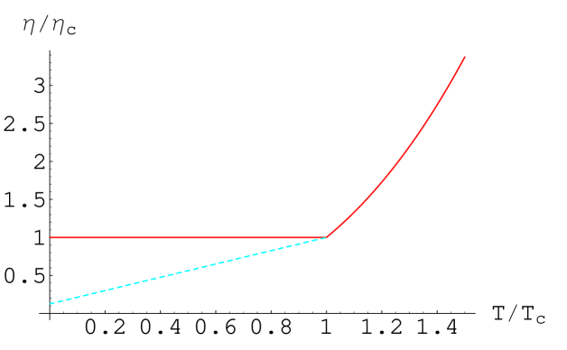
Fig. 2: $\eta/\eta_{c}$ is shown, where $\eta_{c}={\pi N^{2}\over 8}T_{c}^{3}$. Temperature is scaled by $T_{c}$. The dashed line shows the case of T-dependent $r_{m}$ with $T_{c}=270$ MeV.

5 Summary

In this paper we have studied the absorption cross section and viscosity of pure Yang-Mills theory at low temperature where the theory is in the confinement phase. The gluons are confined and we expect that the glueball states are the dominant modes in this phase. In our holographic model, the infrared cutoff $r_{m}$ is introduced as a parameter, and it is fixed by lowest mass of the glueball which is estimated to be about $M_{g}=$ 1.5 GeV. Using this $r_{m}$, the critical temperature of gluon confinement is estimated to be $T_{c}\sim 127$ MeV.

We expect that the thermal properties of the YM theory below $T_{c}$ will be determined by the glueball gas. However, for $T<T_{c}$ the glueball mass is much larger than the temperature, then the glueball gas will not show any active temperature dependence. As expected, we find that both the absorption cross section and the shear viscosity are independent of the temperature. The value of the shear viscosity for $T<T_{c}$ is frozen at the value corresponding to the critical point up to $T=0$. The only possible temperature dependence of the viscosity will be seen through the temperature dependence of the cutoff itself as $r_{m}=r_{m}(T)$. This is an interesting point, to which we will return in the future. But it is an open problem at the present stage.

We have not considered the light flavor quarks and the light mesons constructed by them. If we take into account those mesons, the thermal properties at low temperature will be changed due to the light flavored mesons [18]. This point is also an open problem at the moment.

Finally, let us make some remarks from a fundamental viewpoint on possible physical interpretations of the quantity $r_{m}$. From the above formalism it follows that $r_{m}$ can be looked upon in two different ways. First, $r_{m}$ can be considered to play the role of an extra horizon, in addition to the conventional horizon $r_{0}$ that is present at finite temperature. While Policastro et al. [1] got $\sigma(\omega)\sim\omega^{3}$ for small $\omega$ at $T=0$ and thus $\sigma(0)=0$, we got $\sigma_{\rm IR}$ to be finite at the infrared cutoff (Eq. (14)), at zero temperature. This is to be compared with the result $\sigma(0)=\pi^{3}r_{0}^{3}R^{2}$ in [1], which is finite at finite temperature. Secondly, our result for the shear viscosity at high and low temperature is given by Eqs.(35) and (36). Here, the behaviour of $\eta_{L}$ is seen to be influenced by $r_{m}$. It is of interest to compare also this result with that obtained in [1]: $\eta=f(g^{2}N)N^{2}T^{3}$, where $f(x)$ is a function satisfying $f(x)\sim x^{-2}\ln^{-1}(1/x)$ when $x\ll 1$ and $f(x)=\pi/8$ when $x\gg 1$. We thus see that the quantity $r_{m}$ can manifest itself in different ways physically. It hardly seems possible to associate $r_{m}$ simply with a unique conventional physical quantity.

References

- [1] G. Policastro, D.T. Son and A.O. Starinets, Phys. Rev. Lett. 87, 081601 (2001), hep-th/0104066.
- [2] J. Maldacena, Adv. Theor. Math. Phys. 2, 231 (1998).
- [3] S.S. Gubser, I.R. Klebanov, and A.M. Polyakov, Phys. Lett. B 428, 105 (1998).
- [4] E. Witten, Adv. Theor. Math. Phys. 2, 253 (1998).
- [5] O. Aharony, S.S. Gubser, J. Maldacena, H. Ooguri, and Y. Oz, Phys. Rep. 323, 183 (2000).
- [6] K. Ghoroku and M. Yahiro, Phys. Rev. D 73, 125010 (2006), hep-ph/0512289.
- [7] K. Ghoroku, A. Nakamura and M. Yahiro, Phys. Lett. B 638, 382 (2006), hep-ph/0605026.
- [8] I.R. Klebanov, Nucl. Phys. B496, 231 (1997).
- [9] S.R. Das, G. Gibbons and S.D. Mathur, Phys. Rev. Lett. 78, 417 (1997).
- [10] N. Ishii, H. Suganuma and H. Matsufuru, Phys. Rev. D 66 014507(2002).
- [11] S.S. Gubser, I.R. Klebanov, and A.A. Tseytlin, Nucl. Phys. B499, 217 (1997).
- [12] S.S. Gubser and I.R. Klebanov, Phys. Lett. B 413, 41 (1997).
- [13] G.T. Horowitz and A. Strominger, Nucl. Phys. B 360, 197 (1991).
- [14] M.J. Duff and J.X. Lu, Phys. Lett. B 273, 409 (1991); M.J. Duff, R.R. Khuri, and J.X. Lu, Phys. Rep. 259, 213 (1995).
- [15] A. Hosoya, M. Sakagami, and M. Takao, Ann. Phys. (N.Y.) 154, 229 (1984); see also E.M. Lifshitz and L.P. Pitaevskii, Statistical Physics (Pergamon Press, New York, 1980), Pt. 2, Sec. 90.
- [16] S. Jeon and L.G. Yaffe, Phys. Rev. D 53, 5799 (1996).
- [17] S. Jeon, Phys. Rev. D 52, 3591 (1995).
- [18] J.-W. Chen and E. Nakano, hep-ph/0604138.