Abstract

The role of higher derivative operators in 4D effective field theories is discussed in both non-supersymmetric and supersymmetric contexts. The approach, formulated in the Minkowski space-time, shows that theories with higher derivative operators do not always have an improved UV behaviour, due to subtleties related to the analytical continuation from the Minkowski to the Euclidean metric. This continuation is further affected at the dynamical level due to a field-dependence of the poles of the Green functions of the particle-like states, for curvatures of the potential of order unity in ghost mass units. The one-loop scalar potential in $\lambda\phi^{4}$ theory with a single higher derivative term is shown to have infinitely many counterterms, while for a very large mass of the ghost the usual 4D renormalisation is recovered. In the supersymmetric context of the O’Raifeartaigh model of spontaneous supersymmetry breaking with a higher derivative (supersymmetric) operator, it is found that quadratic divergences are present in the one-loop self-energy of the scalar field. They arise with a coefficient proportional to the amount of supersymmetry breaking and suppressed by the scale of the higher derivative operator. This is also true in the Wess-Zumino model with higher derivatives and explicit soft breaking of supersymmetry. In both models, the UV logarithmic behaviour is restored in the decoupling limit of the ghost.

1 Introduction

Low energy supersymmetry can provide a solution to the hierarchy problem, when this is softly broken at around the TeV scale, and future LHC experiments will be able to test some of the predictions associated with this. In general, low energy models such as Standard Model or its supersymmetric versions, are regarded as effective theories valid up to some high mass scale, at which footprints of a more fundamental theory can show up. These can be in the form of higher dimensional operators, and they can play an important role in clarifying the more fundamental theory valid beyond the high scale, which suppresses their effects at low energies. Usually only non-derivative higher dimensional operators are considered in 4D, while higher derivative ones are less studied or popular, due to many difficult issues involved: either (high scale) unitarity or causality violation, non-locality, the role of the additional ghost fields present in the context of field theories with higher derivative operators (see for example [1]-[25]), etc. Perhaps the most difficult issue in such theories is related to the analytical continuation from the Euclidean to the Minkowski space (or vice-versa) which are not necessarily in a one-to-one correspondence. In this work we attempt to address some of these problems.

Another motivation for studying higher dimension derivative operators in the 4D action comes from the compactification of higher dimensional gauge theories. If physics at low scales is the low-energy limit of a more fundamental such theory, higher derivative operators can be generated dynamically, even in the simplest (orbifold) compactifications. For example, higher derivative operators are generated by gauge (bulk) interactions in 6D at one-loop or 5D beyond one-loop [12, 13, 14, 15]. Brane-localised higher derivative operators are also generated at the loop level [11], by superpotential interactions in 5D or 6D orbifolds. Higher derivative interactions were also studied in the context of Randall-Sundrum models [16]. Therefore, clarifying the role of such operators can help a better understanding of compactification. Further, higher derivative operators are important in other studies: cosmology [17, 18], phase transitions and Higgs mechanism [19, 20, 21], supergravity/higher derivative gravity [22]-[31], string theory [32, 33], used as regularisation method [34], etc. We therefore consider it is worth investigating the role of higher derivative operators in a 4D effective field theory, be it supersymmetric or not.

One common problem in theories with higher derivative operators is that they are in many cases formulated and studied in the Euclidean space, and then it is assumed that there exists an analytical continuation to the Minkowski space. In some simple cases the results of such studies might hold true upon analytical continuation to the Minkowski space. However, in the presence of higher derivative operators, the dispersion relations change, new poles in the fields’ propagators are present, and the position of some of these can move in the complex plane and become field dependent. In this situation, the analytical continuation to Minkowski space becomes more complicated and possibly ambiguous, and one can be faced with difficult choices: different $\pm i\,\epsilon$ prescriptions in the Green functions can lead to different results upon continuation from the Euclidean to the Minkowski space. To avoid this, we start instead with a formulation in the Minkowski space, and pay special attention to this problem. We do so by making the simple observation that the partition function for the second order theory in the Minkowski space, should be well-defined and also recovered from the fourth order Minkowski action, in the decoupling limit of the higher derivative terms, when the scale suppressing these operators is taken to infinity. This is consistent with the finding [2] that a fourth order theory can make sense in Minkowski space if one treats it like a second order theory. Ensuring that the model without higher derivatives (or with their degrees of freedom integrated out) has a well defined partition function in the Minkowski space turns out to be enough to fix the ambiguities mentioned earlier. No special assumptions regarding analytical continuation are made, for this is fixed unambiguously, with some interesting results.

The plan of the paper is the following: we first consider a 4D scalar field theory with a higher derivative term in the action and study its Euclidean and Minkowski formulations and their relationship. Section 2.2 addresses the one-loop effects of higher derivative terms on the scalar field self-energy and scalar potential. We considered interesting to extend the analysis to the supersymmetric case (Section 2.3) and investigate the role of supersymmetric higher derivative terms in the case of O’Raifeartaigh model of spontaneous supersymmetry breaking. We analyse the role of these operators for the UV behaviour of the self-energy of the scalar field. Section 2.4 addresses the same problem in the case of a Wess-Zumino model with supersymmetric higher derivatives terms and explicit soft supersymmetry-breaking terms. In both models it was found that, despite the soft nature of supersymmetry breaking, UV quadratic divergences are generated for the scalar field self-energy, with a coefficient related to the amount of supersymmetry breaking and suppressed by the (high) scale of the higher derivative operator.

2 Effects of Higher Derivative Operators at the loop level.

2.1 A simple example: Higher derivative terms in scalar field theory.

Let us start with a simple 4D toy model with a higher derivative term in the $\lambda\phi^{4}$ theory and study its effects at the classical and quantum level. Our starting point is the 4D Lagrangian

$${\cal L}=-\frac{1}{2}\,\phi\,(\xi\,\Box^{2}+\Box)\,\phi-V(\phi),\qquad\quad V(\phi)\equiv V_{0}+\frac{1}{2}\,(m^{2}-i\,\epsilon)\,\phi^{2}+\frac{\lambda}{4!}\,\phi^{4}$$ (1)

with $\xi\equiv 1/M^{2}_{*}>0$ and $M_{*}$ is some high scale of “new physics” where the higher derivative term becomes important. Our metric convention is $(+,-,-,-)$ and $\Box\equiv\partial_{\mu}\partial^{\mu}$. Additional, higher order derivative terms can be added, but these are suppressed by higher powers of the scale $M_{*}$. In the limit $\xi\rightarrow 0$, the higher derivative terms decouple at the classical level.

The term $+i\,\epsilon\,\phi^{2}$ in ${\cal L}$ (we take $\epsilon>0$) is consistent with the requirement that the partition function for the particle state $\phi$ of the second-order theory (i.e. in the limit $\xi\!=\!0$), as defined in the Minkowski space-time $Z\sim\int D(\phi)\exp(i\int d^{4}x\,{\cal L})$, remains convergent at all momentum scales. The presence of $+i\epsilon\phi^{2}$ is not a choice, it is just the familiar prescription present in ${\cal Z}$ in second order theories. It is then natural to require that this prescription remain valid in our case too (i.e. for non-zero $\xi$) and at all scales, and this is the only assumption we make. This observation is important, for it fixes potential ambiguities present in some treatments of theories with higher order derivatives. Further, in (1) one can change the basis [2] to $\varphi_{1,2}$

$$\varphi_{1,2}=-\frac{(\Box+m_{\pm}^{2}\pm i\,\epsilon^{*}(0))\,\phi\,\sqrt{\xi}}{(m_{+}^{2}-m_{-}^{2}+2i\epsilon^{*}(0))^{1/2}},$$ (2)

where we introduced

$$m_{\pm}^{2}\equiv\frac{1}{2\xi}\Big{[}1\pm(1-4\,\xi\,m^{2})^{\frac{1}{2}}\Big{]}>0,\qquad\epsilon^{*}(0)\equiv\frac{\epsilon}{(1-4\xi m^{2})^{1/2}}>0$$ (3)

Then eq.(1) becomes

$${\cal L}=-\frac{1}{2}\varphi_{1}(\Box+m_{-}^{2}-i\epsilon^{*}(0))\,\varphi_{1}+\frac{1}{2}\varphi_{2}(\Box+m_{+}^{2}+i\,\epsilon^{*}(0))\,\varphi_{2}-\bigg{[}V_{0}+\frac{\lambda}{4!}\,\,\frac{(\varphi_{1}-\varphi_{2})^{4}}{1-4\,\xi\,m^{2}}\bigg{]}$$ (4)

Therefore $\varphi_{2}$ is a ghost, it has the “wrong” sign in front of the kinetic term. Note the presence in the interaction of a coupling between $\varphi_{1}$ and $\varphi_{2}$, which prevents one from ignoring the effects of $\varphi_{2}$. $\varphi_{1,2}$ are not independent degrees of freedom, since $\phi$ and $\Box\phi$ entering their definition are not. In fact only $\phi\propto\varphi_{2}-\varphi_{1}$ exists as an asymptotic state [2]. To conclude, our original field $\phi$ is a “mixing” of particle-like ($\varphi_{1}$) and ghost-like ($\varphi_{2}$) states, eq.(2).

In basis (4) the ghost’ presence is manifest, but for technical reasons it is easier to work in basis (1) where the presence of this degree of freedom is implicit in the propagator of $\phi$ alone, defined by (1). Note the emergence from (1) of $\pm i\epsilon^{*}(0)$ terms in (4), important later on. These are usually overlooked in the literature: if one started instead with action (4) without these prescriptions, one could face a choice ($\pm$) for the prescription in the ghost propagator. In our case these prescriptions are derived from the 4^th order action of (1) which is our starting theory. Further, for fixed $\epsilon\ll 1$, the condition $\epsilon^{*}(0)\ll 1$ requires $m^{2}\xi\ll 1/4$, which we assume to hold true. For model building one would prefer that effects associated with the mass of the ghost (unitarity violation, etc) be suppressed by a high scale, therefore we take $m_{+}^{2}\sim 1/\xi\gg m_{-}^{2}\sim m^{2}$.

In principle one could start with action (4) and insist to have a $-i\epsilon^{*}(0)$ prescription in its ghost term and study such theory; however, with (2) changed accordingly to reflect this, the relation of such theory to (1) is changed: one would obtain in (1) a momentum dependent pole prescription, of type $\epsilon\!\rightarrow\!\epsilon^{\prime}\!=\!\epsilon^{*}(0)(1+\xi\Box)$, unlike in our starting theory (1) where $\epsilon$ is momentum independent. At $p^{2}\!\ll\!1/\xi$ such theory would be similar to (4) (ghost being decoupled), but at $p^{2}\!\gg\!1/\xi$, its partition function for $\phi$ would not remain convergent in Minkowski space, without further assumptions. Such theory can be interesting but will not be discussed in this work.

Let us calculate the one-loop correction to the mass of $\phi$ using the “basis” of eq.(1)

$$-i\,\delta m^{2} = -i\lambda\,\mu^{4-d}\int\frac{d^{d}p}{(2\pi)^{d}}\frac{i}{-\xi p^{4}+p^{2}-m^{2}+i\epsilon}$$ (5)

$$= \frac{-i\lambda\,\mu^{4-d}}{\sqrt{1-4\xi m^{2}}}\int\frac{d^{d}p}{(2\pi)^{d}}\bigg{[}\frac{i}{p^{2}-m_{-}^{2}+i\epsilon^{*}(0)}-\frac{i}{p^{2}-m_{+}^{2}-i\epsilon^{*}(0)}\bigg{]}$$

$$= \frac{-i\lambda\,\mu^{4-d}}{\sqrt{1-4\xi m^{2}}}\int_{\bf E}\frac{d^{d}p}{(2\pi)^{d}}\bigg{[}\frac{1}{p^{2}+m_{-}^{2}}+\frac{1}{p^{2}+m_{+}^{2}}\bigg{]},$$

where the last integral is in the Euclidean space, showed by the index E, while $\mu$ is the standard non-zero finite mass scale introduced by the DR scheme with $d=4-\omega$, $\omega\rightarrow 0$. The above result written instead in a cutoff regularisation makes explicit the nature of (scale) divergence:

$$-i\,\delta m^{2} = \frac{-i\lambda}{(4\pi)^{2}\sqrt{1-4\,\xi\,m^{2}}}\bigg{[}\Big{[}\Lambda^{2}-m_{-}^{2}\ln\Big{(}1+\Lambda^{2}/m_{-}^{2}\Big{)}\Big{]}+\Big{[}\Lambda^{2}-m_{+}^{2}\ln\Big{(}1+\Lambda^{2}/m_{+}^{2}\Big{)}\Big{]}\bigg{]}.$$ (6)

In the formal limit $\xi\rightarrow 0$ i.e. $m_{+}^{2}\gg\Lambda^{2}$, the last two terms (i.e. the ghost correction) cancel against each other, to leave only the particle part, since then $m_{-}^{2}\rightarrow m^{2}$. Note that in any other case, the ghost contributes to the quadratic divergence of the correction. This is important and contradicts the common statement that theories with higher derivative operators have an improved UV regime, as naively expected from power-counting in Minkowski space, first line in eq.(5): this eq would instead suggest a $\ln\Lambda$ divergence only! The explanation of this difference is the plus sign in the last eq above, due to a Wick rotation to Euclidean space, and the two quadratic divergences add up rather than cancel between the two contributions in (5), (6).

As a separate remark, let us also note that if we considered the case of 2 dimensions ($d\rightarrow 2$) naive power counting applied to first line in (5) would suggest the integral is UV finite and yet, the integral is logarithmically divergent in the UV, see the last line in (5). Therefore, it is not only that diagrams that are already UV divergent can turn out to have a worse UV behaviour when Wick rotated to Euclidean space, but also diagrams that appear UV finite by power counting turn out to be UV divergent, with implications for the renormalisation algorithm.

The result also shows that in this simple case the ghost cannot trigger negative (mass)² for the scalar, to bring in an internal symmetry breaking, since here $\delta m^{2}>0$. However this remains a possibility in similar models, if one included additional gauge interactions, fermionic contributions of opposite sign, or other additional 6D operators (such as for example $\phi^{2}\Box\phi^{2}$ with a different coefficient) when more corrections are present and can trigger symmetry breaking.

Let us remark that one can also use a series expansions of the general propagator in the presence of the higher derivative term, and keep only a leading correction:

$$\frac{1}{-\xi\,p^{4}+p^{2}-m^{2}+i\epsilon}=\frac{1}{p^{2}-m^{2}+i\epsilon}+\frac{\xi\,p^{4}}{(p^{2}-m^{2}+i\,\epsilon)^{2}}+{\cal O}(\xi^{2}p^{4})$$ (7)

Here the first term in the rhs is the usual propagator, while the effect of the higher derivative contribution is, to the lowest order, just a small correction. Note however the different number of poles for $p_{0}$ of the lhs and rhs in (7) with implications for continuation from the Minkowski to the Euclidean space. The additional lhs pole, ultimately brings in an additional degree of freedom (ghost), and is present only upon re-summing all higher order terms in the rhs.

The expansion in (7), when performed under a loop integral such as (5), is restrictive for it assumes that one can neglect terms $\xi p^{2}\ll 1$ for any value of $p^{2}$, in particular for $1/\xi\gg p^{2}\sim\Lambda^{2}$ where $\Lambda$ is a UV cutoff of the integral. Using the above expansion in (5) one obtains an approximation (in $\xi$) of the previous result for $\delta m^{2}$, but will be valid only for a ghost mass ($\sim 1/\xi$) much larger than the cutoff scale. This situation is unlike the results of eq.(5), (6), which are more general, being valid for any value of the mass of the ghost ($m_{+}^{2}\sim 1/\xi$) relative to $\Lambda$, in particular for $m_{+}^{2}\sim\Lambda^{2}$, when (7) is not a good approximation since it would require many more terms of the series to be included. To conclude, for applications one should use the full propagator in the presence of higher derivative term and, after that, one can consider special cases such as the limit $m_{+}^{2}\sim 1/\xi\gg\Lambda^{2}$ of decoupling the ghost-like contribution. The advantage of this approach is that one will also be able to consider the case $m_{+}^{2}\sim\Lambda^{2}$ or $m_{+}^{2}<\Lambda^{2}$, (with $m_{+}^{2}$ assumed however much larger than a TeV scale, for phenomenological reasons).

Finally, let us now use the action in eq.(4) and the basis $\varphi_{1,2}$ (instead of $\phi,\Box\phi$), to recover $\delta m^{2}$ of (5). We thus compute at one-loop $\delta m_{\pm}^{2}$ given by interaction (4) proportional to $(\varphi_{1}-\varphi_{2})^{4}$. There are two one-loop diagrams of order $\lambda$ which contribute to $\delta m_{-}^{2}$: one has in the loop a propagator of $\varphi_{1}$, and a symmetry factor 12; the second Feynman diagram has $\varphi_{2}$ in the loop, with a symmetry factor of 2.

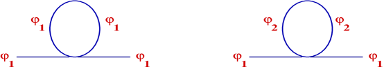
Figure 1: The Feynman diagrams which contribute to the self-energy $\delta m_{-}^{2}$ of the particle-like field $\varphi_{1}$.

The result for $\delta m_{-}^{2}$ is given below:

$$-\frac{i}{2}\,\delta m_{-}^{2}=\frac{-i\lambda}{2}\frac{\mu^{4-d}}{\xi^{2}(m_{+}^{2}-m_{-}^{2})^{2}}\int\frac{d^{d}p}{(2\pi)^{d}}\bigg{[}\frac{i}{p^{2}-m_{-}^{2}+i\epsilon^{*}(0)}+\frac{-i}{p^{2}-m_{+}^{2}-i\epsilon^{*}(0)}\bigg{]}$$ (8)

The minus in front of the last propagator (of $\varphi_{2}$) is explained by the kinetic term for the ghost field $\varphi_{2}$ in (4). The different propagators for $\varphi_{1,2}$ in Minkowski space-time turn out to become identical in Euclidean space-time, see last line in (5). Using that under differentiation of (3)

$$\delta m_{-}^{2}=\frac{\delta m^{2}}{\sqrt{1-4\xi m^{2}}}\,$$ (9)

we obtain a result for $\delta m^{2}$ identical to that in the second line of eq.(5). This confirms that the two descriptions, in terms of $\phi$ or of $\varphi_{1,2}$ are equivalent, as expected. When $\xi\rightarrow 0$, $\delta m_{-}^{2}\rightarrow\delta m^{2}$.

We conclude this section by analyzing what happens if instead of using the Lagrangian in eq.(1),(4), one insists to use instead its Euclidean version, given below

$${\cal L}_{E}=\frac{1}{2}\,\phi\,(\,\xi\Box_{E}^{2}-\Box_{E}+m^{2}\,)\,\phi+\bigg{(}V_{0}+\frac{\lambda^{\prime}}{4!}\,\phi^{4}\bigg{)}$$ (10)

The one-loop result for $\delta m^{2}$ computed with the Feynman rules derived from ${\cal L}_{E}$ gives:

$$-\,\delta m^{2} = -\lambda^{\prime}\,\mu^{4-d}\int_{\bf E}\frac{d^{d}p}{(2\pi)^{d}}\frac{1}{\xi p^{4}+p^{2}+m^{2}}$$ (11)

$$= \frac{-\lambda^{\prime}\,\mu^{4-d}}{\sqrt{1-4\xi m^{2}}}\int_{\bf E}\frac{d^{d}p}{(2\pi)^{d}}\bigg{[}\frac{1}{p^{2}+m_{-}^{2}}-\frac{1}{p^{2}+m_{+}^{2}}\bigg{]}$$

where all $p^{2}$ are evaluated in Euclidean metric, shown by the subscript ${\bf E}$. A similar result is found by working in the corresponding $\varphi_{1,2}$ basis. This result has no quadratic divergence but only a logarithmic one. This would suggest a better UV behaviour of $\delta m^{2}$ in the Euclidean formulation compared to that in (5). Also, eq.(11) with $\lambda^{\prime}\!\rightarrow\!\lambda$ is in contradiction with last line in (5) which has an opposite sign between the contributions from $m_{-}$ and $m_{+}$; this sign was due to two Wick rotations in opposite directions in (5), which brought in an extra (-1) relative sign. Therefore, the origin of this different result is ultimately due to the analytical continuation from the Minkowski to the Euclidean space-time, not captured by the Euclidean formulation alone.

The relation at the loop level, between theories formulated in Euclidean and Minkowski space-time respectively, is further complicated by the fact that if the theory is not renormalisable, a given set of operators (counterterms) in Minkowski space-time may correspond to a different set of operators in the Euclidean spacetime or to the same set but with different coefficients. Also, the Euclidean formulation itself is not always finite. To see these, add in eq.(10) the operator $\Delta{\cal L}_{E}=-z^{\prime}\phi^{2}\Box_{E}\phi^{2}$, ($z^{\prime}>0$) which is dimension 6, like $\phi\Box_{E}^{2}\phi$. Its effect on $\delta m^{2}$ is

$$-\delta m^{2}\Big{|}_{\Delta{\cal L}_{E}}=\frac{-16z^{\prime}\,\mu^{4-d}}{\sqrt{1-4\xi m^{2}}}\int_{\bf E}\frac{d^{d}p}{(2\pi)^{d}}\bigg{[}\frac{m_{+}^{2}}{p^{2}+m_{+}^{2}}-\frac{m_{-}^{2}}{p^{2}+m_{-}^{2}}\bigg{]}$$ (12)

This result shows that the Euclidean theory has quadratic divergences induced by an operator of same dimension as $\phi\Box_{E}^{2}\phi$. Since all operators with same mass dimension should be included for a comprehensive study, it turns out that even the Euclidean formulation of a theory with higher derivatives is not necessarily finite.

The sum of the radiative corrections of (11), (12) gives a result identical to that in (5) of the Minkowski Lagrangian, provided that $\lambda^{\prime}\!=\!\lambda/\sqrt{1-4\xi m^{2}}$ and $z^{\prime}\!=\!\xi\lambda/(16\sqrt{1-4\xi m^{2}})$. For $\xi\!=\!0$ these relations give $\lambda^{\prime}=\lambda$, $z^{\prime}=0$ and the two formulations have identical set of operators and couplings since then the contribution from $m_{+}^{2}\sim 1/\xi$ vanishes. Further, one can also consider the operator $\Delta{\cal L}=-z\phi^{2}\Box\phi^{2}$ in the Minkowski Lagrangian eq.(1) and evaluate its loop corrections to $m^{2}$; after doing so, one obtains similar one-loop corrections to $m^{2}$ in the two formulations from the same set of operators in Minkowski and Euclidean actions (up to a redefinition of their coefficients/couplings). This happens provided that $z^{\prime}=(\xi\lambda/16-z)/\sqrt{1-4\xi m^{2}}$ and $\lambda^{\prime}=(\lambda-64zm^{2})/\sqrt{1-4\xi\,m^{2}}$. This may even lead to $z^{\prime}<0$, for $z>0$, and cause instabilities in the Euclidean theory, present in some theories with higher derivatives.

To conclude, at the loop level the relation between the Euclidean and Minkowski formulations is more complicated in the presence of higher dimensional operators, and in particular higher derivative ones, due to additional poles induced by ghost fields, whose residue affect the analytical continuation. In the following, we restrict the analysis to studying the role of the higher derivative operator only, appearing in eq.(1). A full analysis including all dimension-six operators and their radiative corrections is beyond the goal of this paper.

2.2 The one-loop scalar potential in the presence of higher derivatives

The one-loop scalar potential (vacuum energy) in a 4D theory without higher derivatives is:

$$U(\phi)=V(\phi)-\frac{i\,\mu^{4-d}}{2}\int\frac{d^{d}p}{(2\pi)^{d}}\ln\,\frac{p^{2}-V^{\prime\prime}(\phi)}{p^{2}-V^{\prime\prime}(0)}$$ (13)

with $V(\phi)$ the tree level potential. In string theory the starting point for the vacuum energy is ultimately a somewhat similar formula, “upgraded” to respect string symmetries (world-sheet modular invariance, etc). In the presence of higher derivative terms, eq.(13) is not valid anymore.

Let us address the one-loop potential and its renormalisation in the presence of higher derivatives, using the action in eq.(1). In this case the one-loop potential in the Minkowski space is

$$U(\phi) = V(\phi)-\frac{i\,\mu^{4-d}}{2}\int\frac{d^{d}p}{(2\pi)^{d}}\,\ln\frac{p^{2}-\xi\,p^{4}-V^{\prime\prime}(\phi)+i\epsilon}{p^{2}-\xi\,p^{4}-V^{\prime\prime}(0)+i\epsilon}$$ (14)

$$= V(\phi)-\frac{i\,\mu^{4-d}}{2}\int\frac{d^{d}p}{(2\pi)^{d}}\,\ln\frac{(p^{2}-\alpha_{+}(\phi)-i\,\epsilon^{*}(\phi))}{(p^{2}-\alpha_{+}(0)-i\,\epsilon^{*}(0))}\frac{(p^{2}-\alpha_{-}(\phi)+i\,\epsilon^{*}(\phi))}{(p^{2}-\alpha_{-}(0)+i\,\epsilon^{*}(0))}$$ (15)

where, as usual $\epsilon>0$, and

$$\alpha_{\pm}(\phi)\equiv\frac{1}{2\xi}\Big{(}1\pm\sqrt{1-4\,\xi\,V^{\prime\prime}(\phi)}\,\Big{)},\quad m^{2}_{\pm}=\alpha_{\pm}(0);\quad\epsilon^{*}(\phi)\equiv\frac{\epsilon}{(1-4\,\xi\,V^{{}^{\prime\prime}}(\phi))^{\frac{1}{2}}}$$ (16)

If $\xi V^{{}^{\prime\prime}}(\phi)\ll 1$, $\alpha_{+}(\phi)\approx 1/\xi-V^{\prime\prime}(\phi)$ (ghost-like part), and $\alpha_{-}(\phi)\approx V^{\prime\prime}(\phi)$ (particle-like part).

Note the different $\pm i\epsilon^{*}$ that emerged under the logarithm when going from (14) to (15), with consequences for the analytical continuation to Euclidean space. In many studies, theories with higher derivative operators are studied in Euclidean space and at the end it is assumed that there exists a continuation to the Minkowski space. However, in that case ambiguities (regarding which choice of sign of $i\epsilon$ to take) or additional complications can emerge when going from Euclidean to Minkowski space (see discussion in the previous section). Such issues do not arise when starting with the Minkowski formulation eq.(1) and subsequent (4) and (14). In (1) the $+i\epsilon$ prescription is consistent with a well-defined partition function for the particle-like degree of freedom in Minkowski space, and similar to that for any scalar theory in the absence of higher derivatives ($\xi=0$), considered here a perturbation. Since $\phi$ contains a “piece” of ghost (being a “mixture” of $\varphi_{1,2}$), it is not surprising that this initial prescription implicitly fixes the prescription for the ghost-like part as well; this can be seen in the complex term under the “ghost-like” logarithm in eq.(15), which comes with a definite “prescription” ($-i\epsilon^{*}$).

An intriguing aspect that emerged is the $\phi$ dependence of $\epsilon^{*}$, telling us that the condition $\epsilon^{*}(\phi)$ be very small can be violated at the dynamical level. This should be avoided, at least because otherwise $\alpha_{\pm}(\phi)$ would have values closer to each other and the ghost and the particle reach masses of similar order of magnitude. Then the theory breaks unitarity at a mass scale close to that of the particle and this is not something one would want. One also needs $\alpha_{\pm}(\phi)$ be real, since otherwise the initial fourth order theory would have no particle-like degree of freedom. One would then prefer the ghost have a very large mass, so that effects associated with its mass scale are not present at low energies. Therefore the particle-like degree of freedom is light compared to the ghost-like one, requiring

$$V^{{}^{\prime\prime}}(\phi)\ll\frac{1}{4\,\xi},\qquad{\rm for\,\,\,any}\quad<\phi>$$ (17)

i.e. the curvature of the potential in ghost mass units be smaller than unity; this ensures $\epsilon^{*}\!\ll\!1$.

Let us now discuss the one-loop corrected $U(\phi)$ of (14) which is the sum of two contributions due to $\alpha_{\pm}(\phi)$, each similar to that of a 4D theory without the higher derivative term. Our initial problem of a higher derivative operator in the action is “unfolded” into two 4D copies, each with its own scalar potential(s) with second derivative(s) $\alpha_{\pm}(\phi)$. After a Wick rotation to the Euclidean space, eq.(14) gives

$$U(\phi) = V(\phi)+\frac{\,\mu^{4-d}}{2}\int_{\bf E}\frac{d^{d}p}{(2\pi)^{d}}\,\bigg{[}\ln\frac{(p^{2}+\alpha_{-}(\phi))}{(p^{2}+\alpha_{-}(0))}-\ln\frac{(p^{2}+\alpha_{+}(\phi))}{(p^{2}+\alpha_{+}(0))}\bigg{]}$$ (18)

Notice the minus sign above, consequence of the analytical continuation, and showing the difference between Minkowski and Euclidean spaces properties in higher order theories. If one started the analysis in an Euclidean setup instead, by computing $U(\phi)\sim\mbox{Tr}(\ln[\xi\Box^{2}+\Box+V^{\prime\prime}])$, one would have instead obtained a plus sign in front of the last term in (18)! This difference is due to additional counterterms associated with analytical continuation from Minkowski to Euclidean space, as discussed in the previous section. As a check of the correctness of our result, if one takes the first derivative of $U(\phi)$ with respect to $\phi^{2}$ at $\phi=0$ one recovers exactly $\delta m^{2}$ of eq.(5), (6) in both regularisation schemes. This is a good consistency check.

Eq.(18) tells us something more, when we consider only the field-dependent part of the integrals, involving $\alpha_{\pm}(\phi)$. Each of the integrals gives upon integration a quartic divergence in scale, which may be seen more easily in a cutoff regularisation of (18). From this equation, with a cutoff $\Lambda$ on the above integrals instead of the DR scheme, one has at large $p^{2}$

$$U(\phi) \sim \frac{1}{2}\int_{\bf E}^{\Lambda}\!\!{d^{4}p}\,\Big{[}\ln p^{2}+\alpha_{-}(\phi)\,p^{-2}+\alpha^{2}_{-}(\phi)\,p^{-4}+\cdots\Big{]}-\Big{(}\alpha_{-}\rightarrow\alpha_{+}\Big{)}$$ (19)

The familiar quartic divergence coming from the integration of $\ln p^{2}$ and present in the field dependent part of the particle-like contribution ($\alpha_{-}(\phi)$) is cancelled by the similar one due to its ghost counterpart, from $\alpha_{+}(\phi)$. This cancellation is due to the minus sign in (18), which is in turn due to the rotation from Minkowski to the Euclidean space with opposite prescriptions $\pm i\,\epsilon^{*}$ in (15). The cancellation is similar to that ensured in the presence of softly broken supersymmetry by equal bosonic and fermionic degrees of freedom ${\rm Str}M^{0}=0$. Note however the presence of a UV-finite, cutoff-independent correction, quartic in the mass of the ghost (i.e. in the scale of the higher derivative operators); this comes from $\alpha_{+}^{2}(\phi)\sim 1/\xi^{2}\equiv M_{*}^{4}$ in the limit of small $\xi$. This discussion shows that ultimately higher derivative terms play a role in addressing the cosmological constant problem. These observations and the results of eqs.(4), (15), (18), (19) have some similarities to the proposal in [36] for the cosmological constant.

We now proceed to address the renormalisation of $U(\phi)$. Eq.(18) gives in the DR scheme:

$$U(\phi) = V(\phi)+\Big{[}\Delta U_{1}(\phi)+\Delta U_{2}(\phi)\Big{]}-\Big{[}\Delta U_{1}(0)+\Delta U_{2}(0)\Big{]},$$ (20)

$$\Delta U_{1}(\phi) = c_{o}\,\bigg{[}\frac{1}{\omega}+c_{1}\bigg{]}\bigg{[}\alpha^{2}_{-}(\phi)-\alpha^{2}_{+}(\phi)\bigg{]},\qquad\omega\equiv 4-d\rightarrow 0;$$ (21)

$$\Delta U_{2}(\phi) = \frac{c_{o}}{2}\,\bigg{[}-\alpha_{-}^{2}(\phi)\ln\frac{\alpha_{-}(\phi)}{\mu^{2}}+\alpha_{+}^{2}(\phi)\ln\frac{\alpha_{+}(\phi)}{\mu^{2}}\bigg{]},$$ (22)

where $c_{o}\equiv-1/{2\,(4\pi)^{2}}$,   $c_{1}\equiv{1}/{4}\ln\big{[}(4\pi)^{2}e^{3-2\gamma}\big{]}$.

The contribution $\Delta U_{1}$ involves a square root of the fields, which will require us to introduce infinitely many counterterms, already at the one-loop level. This may be seen from the following equation, valid for $\xi V^{\prime\prime}(\phi)\!\ll\!1$:

$$\alpha^{2}_{-}(\phi)-\alpha^{2}_{+}(\phi)=\,\frac{-1}{\xi^{2}}\,\sqrt{1-4\,\xi\,V^{{}^{\prime\prime}}(\phi)}$$

$$\quad\quad=\,\,-\frac{(1-4\xi m^{2})^{\frac{1}{2}}}{\xi^{2}}+\frac{\lambda\phi^{2}}{\xi\,(1-4\xi m^{2})^{\frac{1}{2}}}+\frac{\lambda^{2}\,\phi^{4}}{2(1-4\xi m^{2})^{\frac{3}{2}}}+\frac{\lambda^{3}\,\xi\,\phi^{6}}{2(1-4\xi m^{2})^{\frac{5}{2}}}+{\cal O}(\xi^{2}\phi^{8})\quad$$ (23)

where we used $V(\phi)$ of (1). The series above requires one introduce higher dimensional counterterms. However, after renormalisation, under the condition $\xi V^{\prime\prime}(\phi)\!\ll\!1$, the usual 4D counterterms are sufficient and the theory “appears” as 4D renormalisable. This condition is respected when the scale of higher derivative operators, $M^{2}_{*}\equiv 1/\xi$ is high enough and when the vev of the field $<\phi>$ has no runaway to infinity. This is exactly our initial condition (17) imposed on physical arguments such as absence of unitarity violation at low scales, etc. In the approximation of neglecting the $\phi^{6}$ counterterm and higher ones, the renormalised potential $U_{r}$ is

$$U_{r}(\phi) = U(\phi)+\delta V_{0}+\frac{\delta m^{2}}{2}\,\phi^{2}+\frac{\delta\lambda}{4!}\,\phi^{4}$$ (24)

$$\frac{\delta\,m^{2}}{2} = -c_{o}\,\lambda\,\,\bigg{[}\frac{1}{\omega}+c_{1}\bigg{]}\,\frac{1}{\xi\,(1-4\,\xi\,m^{2})^{\frac{1}{2}}}+\frac{a_{0}}{2}\,m^{2},$$ (25)

$$\frac{\delta\lambda}{4!} = -c_{o}\,\lambda^{2}\bigg{[}\frac{1}{\omega}+c_{1}\bigg{]}\,\frac{1}{2\,(1-4\,\xi\,m^{2})^{\frac{3}{2}}}+\frac{\lambda}{4!}\,b_{0},\qquad\delta V_{0}=-V_{0}$$ (26)

The cosmological constant term $V_{0}$ only undergoes a finite renormalisation. The mass undergoes renormalisation from both the particle and the higher derivative term (the ghost), which are contributing to the quadratic divergence of the mass. This is seen from the $\xi$ dependence of $\delta m^{2}$; in ordinary $\phi^{4}$ theory, the $\xi$-dependent factor is replaced by $m^{2}$. The coupling constant is also renormalised, despite the presence of the higher derivative term in the action. The coefficients $a_{0}$ and $b_{0}$ account for any finite part of the counterterms, i.e. are regularisation scheme dependent constants, which can be fixed by suitable normalisation conditions. The result is

$$U_{r}(\phi)=\bigg{[}\lambda-\frac{\partial^{4}\Delta U_{2}}{\partial\phi^{4}}\bigg{|}_{\phi=0}\bigg{]}\frac{\phi^{4}}{4!}+\frac{1}{2}\bigg{[}m^{2}-\frac{\partial^{2}\Delta U_{2}}{\partial\phi^{2}}\bigg{|}_{\phi=0}\bigg{]}\phi^{2}+\Delta U_{2}(\phi)-\Delta U_{2}(0)$$ (27)

This is the one-loop scalar potential in the theory with higher derivative term (the derivatives are given in the Appendix eq.(Appendix)). In this very minimal case there is no spontaneous symmetry breaking, (first derivative vanishes only for $\phi=0$), but as mentioned, in models which include additional interactions, fermions, etc., this may be possible. The above form of the one-loop potential can be used in such models. Note that the $\alpha_{+}$ dependent part (ghost contribution) in the last two terms of $U_{r}$ is, at small $\xi$

$$\Delta U_{2}(\phi)-\Delta U_{2}(0)=\alpha^{2}_{+}(\phi)\ln\frac{\alpha_{+}(\phi)}{\mu^{2}}-\alpha^{2}_{+}(0)\ln\frac{\alpha_{+}(0)}{\mu^{2}}\!+\!{\cal O}(\xi^{0})=\frac{\lambda\phi^{2}}{2\,\xi}(2\ln\xi-1)\!+\!{\cal O}(\xi^{0})$$ (28)

where we ignored the $\alpha_{-}$ (particle-like) part which cannot introduce singular terms if $\xi\ll 1$. Note that the quartic mass dependence $1/\xi^{2}=M^{4}_{*}$ present in the field dependent part (from $\alpha^{2}_{+}(\phi)$) is cancelled by that from $\alpha_{+}(\phi=0)$. This leaves only a term proportional to $\phi^{2}/\xi$, which is only quadratic in the (high) mass of the ghost. At non-zero $\phi$ the ghost contribution does not decouple in the potential when $\xi\rightarrow 0$. For smaller $\xi$ the potential acquires a steeper dependence on $\phi$; at large $\xi$ the higher dimensional terms neglected so far become important.

2.3 O’Raifeartaigh supersymmetry breaking with higher derivatives.

We shall now address the implications of the higher derivative operators in a 4D N=1 supersymmetric context. We consider first the case of O’Raifeartaigh model with additional, supersymmetric higher derivative terms and spontaneous supersymmetry breaking. We compute the one-loop correction to the self-energy of a scalar field in the presence of higher derivative operators and investigate its UV behaviour. The action is:

$${\cal L} = \!\int d^{4}\theta\,\sum_{j=0}^{2}\Phi_{j}^{\dagger}\Big{(}1+\xi_{j}\,\Box\Big{)}\Phi_{j}+\bigg{\{}\int d^{2}\theta\bigg{(}\lambda\,\Phi_{0}\,\Phi_{2}+g\,(\Phi_{0}^{2}-M^{2})\,\Phi_{1}\bigg{)}+c.c.\bigg{\}}$$ (29)

$$= \sum_{j=0}^{2}F^{*}_{j}\Big{(}1+\xi_{j}{\Box}\Big{)}\,F_{j}-\varphi^{*}_{j}\Box\Big{(}1+\xi_{j}{\Box}\Big{)}\,\varphi_{j}+i\,\partial_{\mu}\bar{\psi}_{j}\,\bar{\sigma}^{\mu}\Big{(}1+\xi_{j}{\Box}\Big{)}\psi_{j}-\Big{(}g\,M^{2}F_{1}+c.c.\Big{)}$$

$$+ \Big{[}\lambda\Big{(}\varphi_{0}F_{2}+F_{0}\varphi_{2}-\psi_{0}\psi_{2}\Big{)}+g\Big{(}2\varphi_{1}\,\varphi_{0}\,F_{0}+F_{1}\,\varphi_{0}^{2}-2\,\varphi_{0}\,\psi_{1}\,\psi_{0}-\varphi_{1}\,\psi_{0}\,\psi_{0}\Big{)}+c.c.\Big{]}\quad$$

where the chiral superfield $\Phi_{j}$ has components $\Phi_{j}=(\varphi_{j},\psi_{j},F_{j})$. We use standard conventions and for any Weyl spinors $\psi\psi\equiv\psi^{A}\psi_{A}$, $\overline{\psi}\overline{\psi}\equiv\overline{\psi}_{\dot{A}}\overline{\psi}^{\dot{A}}$ and also $\overline{\psi}\,\overline{\sigma}^{\mu}\,\psi\equiv\overline{\psi}_{\dot{A}}\,(\overline{\sigma}^{\mu})^{\dot{A}B}\,\psi_{B}$. The terms involving the $\Box$ operator are manifest supersymmetric if we recall that $-1/16\,{\overline{D}}^{2}\,D^{2}\,\Phi_{j}=\Box\,\Phi_{j}$, for $\Phi_{j}$ a left chiral superfield, and where $D_{A},\,\overline{D}_{\dot{A}}$ are supersymmetric covariant derivatives.

If all $\xi_{j}=0$, $j=0,1,2$ one recovers the familiar O’Raifeartaigh model of supersymmetry breaking. We review this briefly, before returning to the case of non-zero $\xi_{j}$. In this model, take $g,M,\lambda$ all real and non-zero; then the model has spontaneous supersymmetry breaking, since the potential ${\cal V}$ cannot vanish under this assumption. Indeed, the potential is

$${\cal V}=\sum_{i=0,1,2}|F_{i}|^{2}=|\,\lambda\,\varphi_{2}+2\,g\,\varphi_{1}\,\,\varphi_{0}\,|^{2}+|\,g\,(\varphi_{0}^{2}-M^{2})\,|^{2}+\lambda^{2}\,|\,\varphi_{0}\,|^{2}$$ (30)

where $F_{0},F_{1},F_{2}$ are given by the three terms above, in this order. The condition ${\cal V}=0$ has no solution if all $g,M,\lambda$ are non-zero; the minimum conditions $\partial{\cal V}/\partial\varphi_{1,2}=0$ when satisfied, give an extremum value: ${\cal V}_{m}=\lambda^{2}\,|\,\varphi_{0}\,|^{2}+|\,g\,(\varphi_{0}^{2}-M^{2})\,|^{2}$; further, from $\partial{\cal V}_{m}/\partial\varphi_{0}=0$ one obtains that $\varphi_{0}$ is real and that $\varphi_{0}\,(\lambda^{2}+2g^{2}(\varphi_{0}^{2}-M^{2}))=0$. For this equation there are two possibilities: (a): if $\lambda^{2}\geq 2g^{2}M^{2}$ then $\varphi_{0}=0$ and then ${\cal V}_{m}(\varphi_{0}\!=\!0)=g^{2}M^{4}$ is the minimum of the potential and spontaneous supersymmetry breaking takes place. In this case $F_{0}=F_{2}=0$, $F_{1}=g\,M^{2}$. (b): if $\lambda^{2}<2g^{2}M^{2}$, one has two non-zero roots from: $2g^{2}\varphi_{0}^{2}=2g^{2}M^{2}-\lambda^{2}$ which correspond to the minimum of the potential, while ${\cal V}_{m}(\varphi_{0}=0)$ is now a local maximum. In this case ${\cal V}_{m}=g^{2}M^{4}+\varphi_{0}^{2}(\lambda^{2}-2g^{2}M^{2})+g^{2}\varphi_{0}^{4}$ and therefore, in addition to spontaneous supersymmetry breaking, there is internal (spontaneous) symmetry breaking with respect to $\varphi_{0}$ (negative “mass” $\lambda^{2}-2g^{2}M^{2}$). The symmetry of the potential which is broken is a $Z_{2}$ symmetry, $\varphi_{0}\rightarrow-\varphi_{0}$. In this case, $F_{0}=0$, $F_{1}=g(M^{2}-\varphi_{0}^{2})$, $F_{2}=-\lambda\varphi_{0}$ where $\varphi_{0}$ denotes the above non-zero roots. In both cases discussed above, one notices that the condition $gM^{2}=0$ restores supersymmetry and a vanishing ${\cal V}$. This concludes the review of the O’Raifeartaigh model.

We return now to the action in (29) and consider the presence of higher derivatives for some or all superfields. If $\xi_{j}\not\!=\!0$ for some $j$ the corresponding $F_{j}$ field is dynamical and has a ghost field partner ($\Box F_{j}$). The off-shell counting of the bosonic and fermionic real degrees of freedom works as in the absence of the higher derivatives, but now each field has a counterpart (ghost): $\varphi_{j}$ (2), $\Box\varphi_{j}$ (2), $F_{j}$ (2), $\Box F_{j}$ (2), $\psi_{j}$ (4), $\Box\psi_{j}$ (4), since $\Box f$, where $f$ is some field, is seen as an extra degree of freedom, although not independent of $f$ (see discussion around eq.(4)).

In the presence of the higher derivatives ($\xi_{j}\not=0$), the effective potential at the tree level has a minimum which is not affected by the fact that $F_{j}$ has now a dynamical nature. Indeed, the extremum condition $\partial{\cal V}/\partial F_{j}=0$, where ${\cal V}$ is obtained from (29), provides solutions for $F_{j}$, regardless of whether $F_{j}$ is dynamical or not. After inserting back these values of $F_{j}$ in the potential, one obtains for ${\cal V}$ at the extremum point, a result identical to (30), and with squared absolute values of $F_{0,1,2}$ respectively given by the three terms in (30), in this order. With this observation, the discussion of supersymmetry breaking (at the tree level) in the presence of higher derivatives follows identically that after eq.(30) in the absence of higher derivative terms. As before, if $gM^{2}=0$ then supersymmetry is restored.

In this framework we now investigate the UV behaviour of the self energy of scalar field $\varphi_{0}$ in the presence of the higher derivative terms. This is interesting since the supersymmetry breaking is spontaneous, and we would like to see the dependence of the quantum corrections to the mass of $\varphi_{0}$, on the scale of (supersymmetric) higher derivative terms ($1/\xi_{i}$) and on the UV cutoff ($\Lambda$). Does spontaneous supersymmetry breaking remain soft in the presence of higher derivative terms, and if so, under what conditions? These questions are addressed below.

To compute the loop corrections to the mass of $\varphi_{0}$ (see Fig. 2) we first need to replace in (29), $F_{1}\rightarrow\tilde{F}_{1}+gM^{2}$. After this, the new Lagrangian equals ${\cal L}^{\prime}(F_{1}\rightarrow\tilde{F}_{1})+\Delta{\cal L}$ where ${\cal L}^{\prime}$ is that of eq.(29) but without the linear term in $F_{1}$, and

$$\Delta{\cal L}=g^{2}M^{2}\varphi_{0}^{*2}+g^{2}M^{2}\varphi_{0}^{2}-g^{2}M^{4}$$ (31)

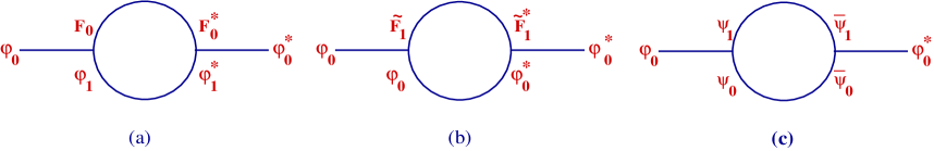
Figure 2: The Feynman diagrams (off-shell) which contribute to the self-energy of $\varphi_{0}$ in Section 2.3.

In the presence of higher derivative terms one must pay attention to the prescriptions for the propagators’ poles. It is easier to understand these by first considering a simpler case, of $\lambda=0,M=0$. In this case

$$<\tilde{F}_{1}\,\tilde{F}_{1}^{*}>=\frac{i}{\xi_{1}\,(\Box+1/\xi_{1}-i\,\tilde{\epsilon})},\qquad<F_{j}\,F_{j}^{*}>=\frac{i}{\xi_{j}\,(\Box+1/\xi_{j}-i\,\tilde{\epsilon})},\qquad j\equiv 0,2$$ (32)

Also

$$\qquad<\varphi_{j}\,\varphi_{j}^{*}> = \frac{-i}{\Box(1+\xi_{j}\Box)-i\epsilon}=\frac{-i}{(\Box-i\epsilon)(1+\xi_{j}\,\Box+i\,\epsilon\,\xi_{j})},\quad\quad j\equiv 0,1,2.$$ (33)

which can further be written as a difference of a particle-like and ghost-like propagators. Finally

$$<\psi^{A}_{j}\overline{\psi}^{\dot{B}}_{j}> = \,\sigma^{\mu\,\,A\dot{B}}\,\,\partial_{\mu}\,\frac{1}{\Box(1+\xi_{j}\,\Box)-i\tilde{\tilde{\epsilon}}},\qquad j=0,1,2.\quad$$ (34)

while $<\overline{\psi}_{\dot{A}}\psi_{B}>$ has a form similar to that of $<\psi^{A}\overline{\psi}^{\dot{B}}>$, but with $\sigma^{\mu\,\,A\dot{B}}$ replaced by $\overline{\sigma}_{\dot{A}B}^{\nu}$. Here we used the indices $A,B=1,2$, $\dot{A},\dot{B}=\dot{1},\dot{2}$. To obtain the momentum representations one replaces $\Box\equiv\partial_{\mu}\partial^{\mu}\rightarrow-p^{2}$ and $\partial^{\mu}\rightarrow-ip^{\mu}$.

The $i\,\epsilon$ prescription for the scalar fields is rather standard, as in the absence of higher derivative operators, and this was discussed in the previous section; the same must be true for fermions, and the prescription we took for their propagator is consistent with a $+i\tilde{\tilde{\epsilon}}\,\psi\,\psi$ shift present in the Minkowski partition function exponent, to ensure its convergence; therefore we have $\tilde{\tilde{\epsilon}}=\epsilon$ ($\epsilon>0$); this is also confirmed later by supersymmetry arguments; however, to be more general, let us keep the sign of $\tilde{\tilde{\epsilon}}$ arbitrary. For the auxiliary fields propagators, comparison of the higher derivative terms for $F_{j}$ in (29) against the second term in (4) suggests that $\tilde{\epsilon}=-\epsilon$ ($\epsilon>0$), but to keep track of its effects, let us keep the sign of $\tilde{\epsilon}$ arbitrary, too.

Returning to the general case of non-zero $\lambda$ and $M$, the propagators change now, due to mass-mixing terms, proportional to $\lambda$, $M$, see (29), (31). An exception is $<\tilde{F}_{1}\,\tilde{F}_{1}^{*}>$ which remains unchanged. For the new propagators that we need in Figure 2, the above prescriptions still apply and are used for the “diagonal entries” in the relevant matrices, as described below. More explicitly, $<F_{0}F_{0}^{*}>$ is now given by the element $({\cal N}^{-1})_{44}$ where ${\cal N}^{-1}$ is the inverse of matrix ${\cal N}$ defined by ${\cal L}\supset(1/2)\,\,\vec{w}\,{\cal N}\,{\vec{w}}^{*\,T}$ with $w$ the vector basis $w\equiv(\varphi_{2}^{*},\varphi_{2},F_{0}^{*},F_{0})$. Similarly, the new propagator $<\varphi_{0}\,\varphi_{0}^{*}>$ is given by the entry $({\cal M}^{-1})_{22}$, where the matrix ${\cal M}$ is read from ${\cal L}\supset(1/2)\,\,\vec{\gamma}\,{\cal M}\,{\vec{\gamma}}^{*\,T}$, with $\vec{\gamma}\equiv(\varphi_{0}^{*},\varphi_{0},F_{2}^{*},F_{2})$. Finally, $<\overline{\psi}_{0}\,\psi_{0}>$ is now given by the element $({\cal P}^{-1})_{11}$ of the inverse matrix ${\cal P}^{-1}$ where ${\cal P}$ can be read from ${\cal L}\supset(1/2)\,\,\vec{\delta}\,{\cal P}\,{\vec{\delta}}^{*\,T}$ with $\vec{\delta}\equiv(\overline{\psi}_{0},\psi_{0},\overline{\psi}_{2},\psi_{2})$. The detailed expressions of these propagators found as described here, are given in the Appendix, eqs.(A-2) to (A-4); these expressions recover, if $\lambda\rightarrow 0,M\rightarrow 0$, those quoted in eqs.(32) to (34), including the prescriptions for the poles.

Using eqs.(A-2) to (A-4), one can evaluate the diagrams which contribute to the mass of $\varphi_{0}$ (Figure 2). The results are

$$(a)\!\!\! = \!\!\!(2ig)^{2}\!\int\!\frac{d^{4}p}{(2\pi)^{4}}\frac{(-1)\,\,(p^{2}\,(1-\xi_{2}p^{2})+i\,\epsilon\,)}{(p^{2}\,(1-\xi_{1}\,p^{2})+i\epsilon)\,\Big{[}\,(1-\xi_{0}\,p^{2}-i\,\tilde{\epsilon}\,\xi_{0})\,\,(p^{2}(1-\xi_{2}\,p^{2})+i\epsilon)-\lambda^{2}\Big{]}}$$

$$(b)\!\!\! = \!\!\!\!\frac{4\,(i\,g)^{2}}{2}\!\!\int\!\!\frac{d^{4}p}{(2\pi)^{4}}\frac{-(1-\xi_{2}\,p^{2}-i\,\tilde{\epsilon}\,\xi_{2})}{(1-\xi_{1}\,p^{2}-i\,\tilde{\epsilon}\,\xi_{1})\,\Big{[}(1-\xi_{2}\,p^{2}-i\,\tilde{\epsilon}\,\xi_{2})\,\,(\,p^{2}\,(1-\xi_{0}\,p^{2})+\rho+i\,\epsilon)\!-\!\lambda^{2}\Big{]}}_{\!\rho=2g^{2}M^{2}}$$

$$\qquad\qquad\quad+\,(\rho\rightarrow-2g^{2}M^{2})$$

$$(c)\!\!\! = \!\!\!(2ig)^{2}\!\int\!\frac{d^{4}p}{(2\pi)^{4}}\frac{2\,p^{2}\,(p^{2}(1-\xi_{2}\,p^{2})+i\tilde{\tilde{\epsilon}})}{(\,p^{2}\,(1-\xi_{1}\,p^{2})+i\,\tilde{\tilde{\epsilon}})\,\,\Big{[}\,(p^{2}(1-\xi_{2}\,p^{2})\!+\!i\tilde{\tilde{\epsilon}})\,\,(p^{2}(1-\xi_{0}\,p^{2})\!+\!i\tilde{\tilde{\epsilon}})-\lambda^{2}\,p^{2}\,]\,\Big{]}}\quad\,\,$$ (35)

We used $tr\,\,[\sigma_{\mu}\,\bar{\sigma}_{\nu}]\partial_{\mu}\,\partial_{\nu}=2\,\Box$ and that diagram (b) has a symmetry factor of 4.

For simplicity consider in the following the case when $\xi_{0}=\xi_{2}=0$, so only the $\Phi_{1}$ superfield has a higher derivative term in (29). We also assume that $1/\xi_{1}\not=\lambda^{2}$, $1/\xi_{1}\not=\lambda^{2}-2g^{2}M^{2}$. (In fact one should take $\xi_{1}\lambda^{2}\ll 1$, $\xi_{1}g^{2}M^{2}\ll 1$ on grounds similar to those discussed in the non-supersymmetric case; here $\lambda$ and $g^{2}\,M^{2}$ play a role similar to $m$ in Section 2.1). One obtains

$$(a) = \,\frac{(2\,i\,g)^{2}}{1-\xi_{1}\,\lambda^{2}}\int\frac{d^{4}p}{(2\pi)^{4}}\,\,\bigg{[}\frac{1}{p^{2}-1/\xi_{1}-i\,\epsilon}-\frac{1}{p^{2}-\lambda^{2}+i\,\epsilon}\bigg{]}$$

$$(b) = \frac{(2\,i\,g)^{2}}{1-\xi_{1}\,\lambda^{{}^{\prime}\,2}}\int\frac{d^{4}p}{(2\pi)^{4}}\bigg{[}\frac{1}{p^{2}-1/\xi_{1}+i\,\tilde{\epsilon}}-\frac{1}{p^{2}-\lambda^{{}^{\prime}\,2}+i\,\epsilon}\bigg{]}\,\frac{1}{2}+\Big{(}\lambda^{{}^{\prime}2}\rightarrow\lambda^{{}^{\prime\prime}2}\Big{)},$$

$$(c) = \frac{(2\,i\,g)^{2}}{1-\xi_{1}\,\lambda^{2}}\int\frac{d^{4}p}{(2\pi)^{4}}\bigg{[}\frac{-2}{p^{2}-1/\xi_{1}-i\,\tilde{\tilde{\epsilon}}}-\frac{-2}{p^{2}-\lambda^{2}+2i\,\tilde{\tilde{\epsilon}}}\bigg{]}$$ (36)

where we introduced $\lambda^{{}^{\prime}\,2}\equiv\lambda^{2}-2g^{2}M^{2}$ and $\lambda^{{}^{\prime\prime}\,2}\equiv\lambda^{2}+2g^{2}M^{2}.$

If $\xi_{1}=0$ then the usual cancellations for spontaneously broken supersymmetry are present, with no quadratic divergences, and only logarithmic terms (in UV cutoff) present. To see this, note that in this limit the first term in every square bracket in (2.3) vanishes, and any contributions from corresponding ghost fields are decoupled. The second term in any of the above brackets represents the usual contribution in the absence of higher derivative terms, with overall $\xi_{1}$-dependent coefficients equal to unity when $\xi_{1}=0$. This supersymmetric cancellation is consistent with the prescription $\tilde{\tilde{\epsilon}}>0$ and $\tilde{\epsilon}<0$ as stated after eq.(34).

For non-zero $\xi$, the ghost-like fields contribute to the radiative corrections and to their UV behaviour; also, in this case the coefficients of the “normal” contributions (for $\xi_{1}=0$) are now multiplied by $\xi$-dependent factors, different from 1. In this case, and using the notation $\tilde{\epsilon}=v\,\epsilon$, $\tilde{\tilde{\epsilon}}=u\,\epsilon$, (where $v=-1,\,u=1$), the result of adding the (a), (b), (c) contributions is

$$\Delta m^{2}_{\varphi_{0}} = \frac{g^{2}}{4\pi^{2}}\,\bigg{\{}\bigg{[}\frac{2(1-2u)}{1-\xi_{1}\,\lambda^{2}}+\frac{1-v}{2(1-\xi_{1}\,\lambda^{{}^{\prime}\,2})}+\frac{1-v}{2(1-\xi_{1}\,\lambda^{{}^{\prime\prime}\,2})}\bigg{]}\,\Lambda^{2}+\frac{(1-2u)}{1-\xi_{1}\lambda^{2}}\,\,g(\Lambda^{2},\lambda^{2})$$ (37)

$$+ \bigg{[}\frac{1-2\,u}{1-\xi_{1}\lambda^{2}}-\frac{v/2}{1-\xi_{1}\,\lambda^{{}^{\prime}\,2}}-\frac{v/2}{1-\xi_{1}\,\lambda^{{}^{\prime\prime}\,2}}\bigg{]}\,g(\Lambda^{2},1/\xi_{1})+\bigg{[}\frac{g(\Lambda^{2},\lambda^{{}^{\prime}\,2})}{2\,(1-\xi_{1}\lambda^{{}^{\prime}\,2})}+(\lambda^{\prime}\rightarrow\lambda^{{}^{\prime\prime}})\bigg{]}\quad$$

with $g(\Lambda^{2},m^{2})=-m^{2}\ln(1+\Lambda^{2}/m^{2})$. The above expression becomes (with $v=-1,\,u=1$)

$$\Delta m^{2}_{\varphi_{0}} = \frac{g^{2}}{4\pi^{2}}\frac{2\,\xi_{1}^{2}\,(2g^{2}M^{2})^{2}}{(1-\xi_{1}\,\lambda^{2})\,(1-\xi_{1}\,\lambda^{{}^{\prime}2})\,(1-\xi_{1}\,\lambda^{{}^{\prime\prime}2})}\,\,\Lambda^{2}+{\cal O}(\ln\Lambda)$$ (38)

with the notation $\lambda^{{}^{\prime}\,2}\equiv\lambda^{2}-2g^{2}M^{2}$ and $\lambda^{{}^{\prime\prime}\,2}\equiv\lambda^{2}+2g^{2}M^{2}.$

Before addressing the result obtained, let us remind that the “prescriptions” we took $v=-1$, $u=1$ or equivalently $\tilde{\epsilon}=-\epsilon$ and $\tilde{\tilde{\epsilon}}=\epsilon$, are those stated in the text after eq.(34), and it is re-assuring to know that they are also consistent with supersymmetry arguments and cancellations that take place for exact supersymmetry, as discussed earlier. One may ask whether the other “possibilities” could be correct, such as $v=1,\,u=\pm 1$ or $v=-1,u=-1$? The answer is negative, and they can be easily ruled out; for example, if supersymmetry is exact ($M=0$) or only softly broken but without higher derivatives ($\xi_{1}=0$), the sum of quantum corrections would still have quadratic divergent terms for these “choices”, which is clearly not allowed.

According to (38), we find the interesting result that supersymmetry breaking, although spontaneous, can nevertheless bring in quadratic divergences at one-loop, if higher derivative supersymmetric terms are present in the initial action. This result is not in contradiction with soft supersymmetry breaking theorems [37], which do not include higher dimensional derivative supersymmetric terms.

The quadratic divergence found for $\Delta m_{\varphi_{0}}^{2}$ has a coefficient that is proportional to $g^{4}M^{4}$ which is related to the “amount” of supersymmetry breaking, and inverse proportional to the mass scale of the higher derivative operators $M_{1,*}^{2}\equiv 1/\xi_{1}$. If $\xi_{1}$ is small enough i.e. the scale of higher derivative operator is high (required in the end for model building, phenomenology, reasons of unitary, etc), the quadratic divergence has a smaller coefficient, but it is still present. In the special limit of decoupling the higher derivative operators ($\xi\,\Lambda^{2}\ll 1$) we recover the usual result that no quadratic divergences are present in spontaneous supersymmetry breaking, in the absence of higher derivative terms in the action.

Another case one can consider is $\xi_{0}=\xi_{1}=\xi_{2}\equiv\xi$, when all fields in the model have higher derivative operators, and all auxiliary fields are dynamical. The one-loop correction of eq.(2.3) becomes

$$(a) = \!(2ig)^{2}\int\frac{d^{4}p}{(2\pi)^{4}}\frac{-1}{\Big{(}1-\xi\,p^{2}-i\,\xi\,\tilde{\epsilon}\,\Big{)}\,\Big{(}\,p^{2}\,(1-\xi\,p^{2})+i\,\epsilon\Big{)}-\lambda^{2}}$$

$$(b)\!\! = \!\!\frac{(2i\,g)^{2}}{2}\!\!\int\frac{d^{4}p}{(2\pi)^{4}}\!\frac{-1}{\Big{(}1-\xi p^{2}-i\,\xi\,\tilde{\epsilon}\,\Big{)}\,\Big{[}(p^{2}\,(1-\xi\,p^{2})+i\epsilon)+\rho\,\Big{]}-\lambda^{2}}\bigg{|}_{\rho=2g^{2}M^{2}}\!\!\!\!+\Big{[}\rho\rightarrow-2g^{2}M^{2}\Big{]}$$

$$(c) = (2i\,g)^{2}\int\frac{d^{4}p}{(2\pi)^{4}}\frac{2}{p^{2}\,(1-\xi\,p^{2})^{2}+2\,i\tilde{\tilde{\epsilon}}\,(1-\xi\,p^{2})-\lambda^{2}}\,$$ (39)

The result of evaluating these integrals is given in Appendix, eqs.(A-5)-(A-12). We take into account that $\tilde{\epsilon}=-\epsilon<0$ and $\tilde{\tilde{\epsilon}}=\epsilon>0$ which are important for the UV behaviour, as they involve different Wick rotations and thus additional minus relative signs. We provide below the result in the limit when $\xi\lambda^{2}\ll 1$ and $\xi\,g^{2}\,M^{2}\ll 1$. After adding together the contributions above, one has

$$\Delta m_{\varphi_{0}}^{2}=\frac{5\,g^{2}}{\pi^{2}}\,\,\,(2g^{2}\,M^{2})^{2}\,\xi^{2}\,\Lambda^{2}+{\cal O}(\ln\Lambda)$$ (40)

Similar to the case of non-vanishing $\xi_{1}$, we found that in the presence of supersymmetric higher derivative operators, supersymmetry breaking - although spontaneous - brings in, nevertheless, a quadratic divergence to the one-loop self energy of the scalar field. In the limit of restoring supersymmetry ($gM=0$), the quadratic divergence is absent, as it should be the case. Also, in the special case of decoupling of the higher derivative operators when their scale is much larger then the UV scale (i.e. $\xi\Lambda^{2}\ll 1$) this divergence is again absent, as expected.

In conclusion and somewhat surprisingly, spontaneous supersymmetry breaking in the presence of higher derivative supersymmetric operators is no longer soft and quadratic divergences are present, with a coefficient equal to the ratio of the parameter related to the amount of supersymmetry breaking and the scale of higher derivative operators. The need for a high scale of the higher derivative operators discussed earlier, ensures ultimately a small value of the coefficient of the quadratic divergences. Moreover, the quadratic divergence has a coefficient which is suppressed by the power 4 of the scale $M_{*}\equiv 1/\sqrt{\xi}$ of the higher derivative operator.

2.4 Wess-Zumino model with soft breaking terms and higher derivatives.

In this section we investigate the extent to which our previous findings for the supersymmetric case remain true in the case of explicit breaking of supersymmetry, as opposed to the spontaneous breaking analysed. We consider the Wess-Zumino model with a soft breaking term and extended with supersymmetric higher derivative operators. We examine the one-loop self-energy of the scalar field. The action is

$${\cal L} = \int d^{4}\theta\,\Phi^{\dagger}\Big{(}1+\xi\,\Box\Big{)}\Phi+\bigg{\{}\int d^{2}\theta\bigg{(}\frac{1}{2}\,m\Phi^{2}+\frac{1}{3}\lambda\,\Phi^{3}\bigg{)}+c.c.\bigg{\}}-m^{2}_{0}\,\varphi\,\varphi^{*}$$ (41)

$$= F^{*}\Big{(}1+\xi{\Box}\Big{)}\,F-\varphi^{*}\Box\Big{(}1+\xi{\Box}\Big{)}\,\varphi+i\partial_{\mu}\bar{\psi}\,\bar{\sigma}^{\mu}\Big{(}1+\xi{\Box}\Big{)}\psi$$

$$+ \Big{(}\,\frac{1}{2}m\,\big{(}2\varphi\,F-\psi\psi\big{)}+\lambda\,\big{(}\varphi^{2}\,F-\varphi\,\psi^{2}\big{)}+c.c.\Big{)}-m^{2}_{0}\,\varphi\,\varphi^{*}$$

with $\Phi\equiv(\varphi,\psi,F)$ and a notation similar to that in the O’Raifeartaigh model.

The last term in (41) breaks supersymmetry softly. The field $F$ is dynamical and has a ghost field partner ($\Box F$). The off-shell counting of the bosonic and fermionic real degrees of freedom works as in the usual Wess-Zumino model, but now each field has a (ghost) counterpart: $\varphi$ (2), $\Box\varphi$ (2), $F$ (2), $\Box F$ (2), $\psi$ (4), $\Box\psi$ (4).

The relevant propagators in the presence of higher derivative term are found as in previous section. For example one writes the quadratic terms in the action in basis $\vec{\sigma}\equiv(\varphi,F^{*})$ as ${\cal L}=(1/2)\,\vec{\sigma}\,{\cal M}\,\vec{\sigma}^{*T}$ and then invert the matrix ${\cal M}$. One finds

$$<\varphi\,\varphi^{*}> = \frac{-i\,(1+\xi\Box-i\,\tilde{\epsilon}\,\xi)}{[\,\Box(1+\xi\Box)+m_{0}^{2}-i\epsilon]\,(1+\xi\Box-i\,\tilde{\epsilon}\,\xi)\,+m^{2}},$$

$$<F\,F^{*}> = \frac{i\,(\Box\,(1+\xi\Box)+m_{0}^{2}-i\,\epsilon)}{[\,\Box(1+\xi\Box)+m_{0}^{2}-i\epsilon]\,(1+\xi\Box-i\,\tilde{\epsilon}\,\xi)\,+m^{2}},$$ (42)

with our usual convention that $\epsilon>0$. In the above eqs, the $i\epsilon$-prescription is in agreement with that for $\xi=0$ and ultimately read from that of the propagator of $\varphi$ alone (with $m=0$), entering the mass mixing matrix; there is also a $i\tilde{\epsilon}$ prescription, which originates from the propagator for the $F$ field in the absence of any mixing by $m$. For the propagator of the field $F$, comparison of the higher derivative terms in Wess-Zumino model against the second term in (4) suggests that $\tilde{\epsilon}=-\epsilon$; let us however keep the sign of $\tilde{\epsilon}$ arbitrary, as we did in the O’Raifeartaigh model. Finally, eqs.(2.4) are written in the presence of the supersymmetry breaking term, while if supersymmetry is unbroken one simply sets $m_{0}=0$. For fermions one finds the propagator

$$<\psi^{A}\overline{\psi}^{\dot{B}}> = (1+\xi\,\Box)\,\sigma^{\mu\,\,A\dot{B}}\,\,\partial_{\mu}\,\frac{1}{\Box(1+\xi\,\Box)^{2}+m^{2}-2\,i\,\tilde{\tilde{\epsilon}}\,(1+\xi\,\Box)},$$ (43)

A similar expression exists for $<\overline{\psi}_{\dot{A}}\psi_{B}>$, but with the matrix $\sigma^{\mu\,\,A\dot{B}}$ replaced by $\overline{\sigma}_{\dot{A}B}^{\mu}$. For the fermionic propagators, the prescription is $\tilde{\tilde{\epsilon}}=\epsilon>0$, and is found similarly to the O’Raifeartaigh model. In the limit $\xi=0$ one recovers the usual propagator for Weyl fermions.

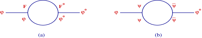
Figure 3: The one-loop Feynman diagrams (off-shell) which contribute to the scalar field self-energy for scalar field $\varphi$, in the Wess-Zumino model with higher derivative terms.

Using these propagators, one obtains the following one-loop contributions, see Figure 3, to the mass of the scalar field $\varphi$, for vanishing external momentum:

$$(a) = 4\,\,(i\lambda)^{2}\,\,\int\frac{d^{d}p}{(2\pi)^{d}}\frac{-(1-\xi\,p^{2}-i\,\tilde{\epsilon}\,\xi)\,[\,p^{2}(1-\xi\,p^{2})-m_{0}^{2}+i\,\epsilon\,]}{[\,(\,p^{2}(1-\xi\,p^{2})-m_{0}^{2}+i\,\epsilon)\,\,(1-\xi\,p^{2}-i\,\tilde{\epsilon}\,\xi)-m^{2}\,]^{2}}$$ (44)

$$(b) = -2\,\,(-i\lambda)^{2}\int\frac{d^{d}p}{(2\pi)^{d}}\frac{(1-\xi\,p^{2})^{2}\,\,tr(\sigma^{\mu}\overline{\sigma}^{\nu})(-p_{\mu}p_{\nu})}{[\,p^{2}\,(1-\xi\,p^{2})^{2}-m^{2}+2\,i\,\tilde{\tilde{\epsilon}}\,(1-\xi\,p^{2})]^{2}},$$ (45)

for bosons and fermions respectively, with $tr(\sigma^{\mu}\overline{\sigma}^{\nu})=2\,\eta^{\mu\nu}$.

For our purposes of investigating the UV behaviour of the self-energy correction, it is sufficient to consider the massless case, $m=0$, when the above loop integrals simplify considerably, without changing their UV behaviour. In that case we have,

$$(a) = 4\,\,(i\lambda)^{2}\,\,\int\frac{d^{d}p}{(2\pi)^{d}}\frac{-1}{(-\xi)\,\,[\,p^{2}(1-\xi\,p^{2})-m_{0}^{2}+i\,\epsilon]\,(p^{2}-1/\xi+i\,\tilde{\epsilon}\,\,)},\qquad(\tilde{\epsilon}=-\epsilon)$$

$$(b) = 2\,\,(-i\lambda)^{2}\int\frac{d^{d}p}{(2\pi)^{d}}\frac{2}{(-\xi)\,\,[\,p^{2}(1-\xi\,p^{2})+2\,i\,\tilde{\tilde{\epsilon}}]\,(p^{2}-1/\xi-2\,i\,\tilde{\tilde{\epsilon}}\,\,)},\qquad\quad(\tilde{\tilde{\epsilon}}=\epsilon)$$ (46)

One again observes that if supersymmetry is restored, one must have that $\tilde{\epsilon}=-\tilde{\tilde{\epsilon}}=-\epsilon$, which is consistent with our choice and as already encountered in the O’Raifeartaigh model.

Remembering that (a) and (b) are contributions to $-i\Delta m_{\varphi}^{2}$, we find

$$\Delta m^{2}_{\varphi} = \!\!\frac{\lambda^{2}}{4\pi^{2}}\,\,\bigg{\{}(3\,\xi\,m_{0}^{2})\,2\Lambda^{2}-m_{0}^{2}\,\,\Big{[}\ln(1+\xi\,\Lambda^{2})-\frac{\sigma}{2}\,(\sigma-4)\Big{]}-m_{0}^{2}\,(1+4\xi\,m_{0}^{2})\,\ln(1+\Lambda^{2}/m_{0}^{2})$$ (47)

$$\quad+\,\bigg{[}\,\frac{m_{0}^{2}\,\Lambda^{2}}{\Lambda^{2}+m_{0}^{2}}-\frac{m_{0}^{2}}{3}\Big{(}\sigma\,(18-6\,\sigma+\sigma^{3})+12\,\ln(1+\Lambda^{2}\,\xi)\Big{)}\bigg{]}\,\xi\,m_{0}^{2}+{\cal O}\Big{(}(\xi\,m_{0}^{2})^{2}\Big{)}\bigg{\}}$$

where $\sigma=\Lambda^{2}\xi/(1+\Lambda^{2}\xi)$. This result is valid for $\xi\,m_{0}^{2}\ll 1$, but for an arbitrary relation between $\Lambda$ and $\xi$. For the result without this approximation see the Appendix, eq.(A-13).

We therefore obtain, similar to the case of the O’Raifeartaigh model, that a quadratic divergence is present in the overall bosonic and fermionic contributions, equal to $(3\,\xi\,m_{0}^{2})\,2\Lambda^{2}$. All the remaining terms in (47) arise from expansions (for $\xi m_{0}^{2}\ll 1$) of logarithms of arguments involving ratios of $\Lambda^{2}$ and mass terms function of $\xi$ and $m_{0}^{2}$. The quadratic divergence is present despite the soft nature of supersymmetry breaking, and is due to the fact that we considered this breaking in the presence of higher derivative supersymmetric terms. In the limit of restoring supersymmetry, $m_{0}\rightarrow 0$ this divergence and in fact the entire quantum correction is absent, as expected. The coefficient of our quadratic divergence is proportional to the amount of supersymmetry breaking ($m_{0}$), and inverse proportional to the scale $M_{*}^{2}=1/\xi$ of the higher derivative operator. These results remain valid in the case of a non-zero mass shift $m$ for fermions/bosons.

It is worth noticing that, unlike the case of O’Raifeartaigh model, in the present case the coefficient of the quadratic divergence is less suppressed, by $M_{*}^{2}$ ($M^{2}_{*}=1/\xi$), rather than $M_{*}^{4}$. The origin of this difference can be traced back to the presence in the Wess Zumino-model of the soft breaking term $m_{0}^{2}\,\varphi\,\varphi^{*}$, while in the spontaneous breaking, its counterpart involved a bilinear term $g^{2}M^{2}\varphi_{0}^{2}+c.c.$ rather than $g^{2}M^{2}\varphi_{0}\varphi_{0}^{*}$, see (31).

Let us finally take the special limit $\xi\,\Lambda^{2}\ll 1$, which decouples the higher derivative operators in the classical action. In this case only a logarithmic correction (in the UV cutoff) survive in (47) of type $-m_{0}^{2}\ln(1+\Lambda^{2}/m_{0}^{2})$, the higher derivative operator and associated ghost fields contributions decouple, to recover that no quadratic divergences are present [37] in softly broken supersymmetry in an action without higher dimensional terms.

We conclude this section with a remark which applies to both O’Raifeartaigh and Wess-Zumino models. Our analysis is somewhat restrictive in that we considered only the role of one particular higher dimension (derivative) operator on the UV behaviour of the scalar field; however, other operators of same or lower mass dimension can be present and should be included for a complete study, with possibly different conclusions. For example one can have additional operators such as $\int d^{2}\theta\Phi\Box^{2}\Phi$ or $\int d^{4}\theta(\Phi^{\dagger}\Phi)^{2}$, suppressed by additional powers of a mass scale. Such new scale introduces additional parameters in the theory, unless this is taken equal to $M_{*}$. Such terms can change significantly our one-loop results and bring in additional, interesting effects.

3 Final Remarks and Conclusions

In this work we discussed the role that higher derivative operators play at the quantum level, and their implications, for both non-supersymmetric and supersymmetric 4D theories. Such operators are in general expected in effective theories, and in models of compactification and this motivated this study, despite the problems that theories with higher derivative operators may have.

We first considered a 4D scalar field theory with higher derivatives, and stressed the important role of a well-defined partition function in the Minkowski space at all momentum scales, for loop calculations and for analytical continuation to the Euclidean space to exist and be unambiguously defined. The loop corrections to the self-energy of the scalar field were computed in the presence of higher derivative terms, to show that these do not necessarily improve the UV behaviour of the theory, as usually considered. This is because Minkowski space-time power-counting criteria for convergence do not always remain true in higher order theories. The reason for this is the relation Minkowski-Euclidean analytical continuation, which involves Wick rotations in opposite senses, such that ultimately ghost-like and particle-like degrees of freedom contributions add up (rather than cancel) to the UV behaviour of the scalar field self-energy.

We also discussed the relation between a Minkowski and an Euclidean theory both with higher derivative terms, and similar action at the tree level, to show that their relation is complicated at loop level by the presence of higher derivative terms. This complication arises due to the additional poles that higher derivative terms induce in the Minkowski spacetime. As a result of their presence, the two theories can give similar result for the one-loop self energy, although they do not have an identical set of operators or these can come with different coefficients. It also turns out that not even the Euclidean theory with higher derivatives is finite or only logarithmic divergent. Instead, it can also have quadratic divergences in the case that other dimension six-operators are included, in addition to the higher derivative kinetic term.

The analytical continuation of our loop corrections derived in the Minkowski space-time is further affected at the dynamical level due to a field-dependence of the poles of the Green functions of the particle-like states, for curvatures of the potential of order unity in ghost mass units. The one-loop scalar potential in $\lambda\phi^{4}$ theory in the presence of a single higher derivative operator is shown to have infinitely many counterterms, while for a large mass of the ghost the usual 4D renormalisation is recovered. There exists an interesting cancellation of the quartic divergence in the (field dependent part of the) one-loop potential, between the scalar field and its ghost counterpart contributions, and this suggests that the higher derivative operators may play a role for the cosmological constant problem. The cancellation is a property specific to the Minkowski space-time formulation of the theory and its partition function convergence, and is absent in a counterpart Euclidean theory with higher derivatives.

Our study also considered supersymmetric models with higher derivative terms in the action. In the case of O’Raifeartaigh models with spontaneous supersymmetry breaking and (supersymmetric) higher derivative terms it was shown that, despite the soft nature of the breaking, quadratic divergences are nevertheless present. The coefficient of this divergence is given by the ratio of the amount of supersymmetry breaking to the scale of higher derivative operators, and thus vanishes when restoring supersymmetry or when decoupling the higher derivative terms. Similar results hold true in the case of Wess-Zumino model with higher derivative terms and soft (in the traditional sense), explicit supersymmetry breaking terms and this was investigated in detail. The emergence of these quadratic divergences is related to the presence of ghost fields in the loop corrections; these corrections vanish when such fields acquire a mass much larger than the UV cutoff scale (the decoupling limit) and then softly broken supersymmetry is restored.

Although our work considered toy-models only, it may be interesting to think of the implications of these findings for phenomenology and for the hierarchy problem in realistic models. Despite many problems that theories with higher derivative terms may have conceptually or phenomenologically (their stability, possible unitarity violation, etc) let us compare the leading correction $\xi\,m_{0}^{2}\,\Lambda^{2}$ found for the scalar field self-energy in Wess-Zumino model, against its counterpart in the supersymmetric versions of the Standard Model, equal to $m_{0}^{2}\ln\Lambda^{2}/m_{0}^{2}$, (we assume similar values for the soft mass $m_{0}$). The two corrections would be of similar order of magnitude provided that $\xi\Lambda^{2}\sim{\cal O}(10-100)$. This would set the scale of the higher derivative operator within a factor of 10 or so below the cutoff scale/Planck scale. Such scale can be high enough to remove any conceptual problems that higher derivative operators might bring. In the case of O’Raifeartaigh models of supersymmetry breaking, comparing the one-loop correction to the scalar field mass, which is $(\xi\,m_{0}^{2})^{2}\,\Lambda^{2}$ to $m_{0}^{2}\ln\Lambda^{2}/m_{0}^{2}$, gives $\xi\,\Lambda\sim{\cal O}(10^{-5}-10^{-4})\,GeV^{-1}$ after assuming a TeV-scale value for $m_{0}$. As a result, in this case the scale of higher derivative operators can be significantly lower, in the range of intermediate energies, ${\cal O}(10^{11}-10^{12})$ GeV.

The results obtained in this work may be extended to higher dimensional theories with various supersymmetry breaking mechanisms, in the presence of higher derivative operators on the “visible” brane or in the bulk. This is interesting since such operators can be generated dynamically during compactification, thus their effects need to be taken into account. It is likely that the supersymmetry breaking effects seen here are present in such theories too, with potentially interesting implications for theory and phenomenology.

Acknowledgements: D.G. thanks Hyun Min Lee (DESY) for many interesting and useful discussions on higher derivative theories and research collaboration on related topics. D.G. acknowledges the financial support from the RTN European Program MRTN-CT-2004-503369 “The Quest for Unification” to attend the “Planck 2006” conference (Paris, May 2006) where part of this work was completed. This work was supported in part by the European Commission under the RTN contracts MRTN-CT-2004-503369, MRTN-CT-2004-005104, the European Union Excellence Grant, MEXT-CT-2003-509661, CNRS PICS no. 2530 and 3059 and in part by the INTAS contract 03-51-6346.

Appendix

I. We have the following derivatives for the scalar potential obtained in the text, eq.(27)

$$\frac{\partial^{2}\Delta U_{2}(\phi)}{\partial\phi^{2}}\bigg{|}_{\phi=0} = \frac{-\lambda\,c_{o}}{2\xi(1-4\,\xi\,m^{2})^{1/2}}\bigg{[}2\,\xi\,m_{-}^{2}\ln\frac{m_{-}^{2}}{\mu^{2}}+2\,\xi\,m^{2}_{+}\ln\frac{m^{2}_{+}}{\mu^{2}}+1\bigg{]}$$

$$\frac{\partial^{4}\Delta U_{2}(\phi)}{\partial\phi^{4}}\bigg{|}_{\phi=0} = \frac{-3\,\lambda^{2}\,c_{o}}{(1-4\,\xi\,m^{2})^{3/2}}\bigg{[}1+\,\ln\frac{m^{2}}{\xi\,\mu^{4}}\bigg{]}$$ (A-1)

II. The propagators used in the case of the O’Raifeartaigh model, eqs.(2.3), are given below. For $\lambda=0$, $M=0$ one recovers the propagators in the absence of mass mixing terms, given in eqs.(32) to (34), together with their prescriptions for the poles. The results are:

$$<F_{0}\,F_{0}^{*}>=i\,\frac{\Box(1+\xi_{2}\,\Box)-i\epsilon}{\Big{(}\Box(1+\xi_{2}\,\Box)-i\,\epsilon\Big{)}\Big{(}1+\xi_{0}\Box-i\,\tilde{\epsilon}\,\xi_{0}\Big{)}+\lambda^{2}}$$ (A-2)

and

$$<\varphi_{0}\,\varphi_{0}^{*}>=\frac{-i\,(1+\xi_{2}\,(\Box-i\,\tilde{\epsilon}\,))\,\,[\lambda^{2}+(1+\xi_{2}\,(\Box-i\,\tilde{\epsilon}))\,\,(\Box(1+\xi_{0}\Box)-i\,\epsilon)\,]}{[\lambda^{2}+(1+\xi_{2}\,(\Box-i\,\tilde{\epsilon}))\,\,(\Box(1+\xi_{0}\,\Box)-i\,\epsilon)\,]^{2}-(2g^{2}M^{2})^{2}\,(1+\xi_{2}\,(\Box-i\,\tilde{\epsilon}))^{2}}$$ (A-3)

Finally

$$<\overline{\psi}_{0}\psi_{0}>=\frac{\partial\!\!/\,[\Box\,(1+\xi_{2}\,\Box)-i\,\tilde{\tilde{\epsilon}}\,]}{(\Box\,(1+\xi_{0}\,\Box)-i\,\tilde{\tilde{\epsilon}}\,)\,[\,\Box\,(1+\xi_{2}\,\Box)-i\,\tilde{\tilde{\epsilon}}\,]+\lambda^{2}\,\Box}$$ (A-4)

where $\not\!\!\partial\equiv\partial^{\mu}\sigma_{\mu}$. Above we used $<F_{0}F_{0}^{*}>=({\cal N}^{-1})_{44}$ where ${\cal N}^{-1}$ is the inverse of matrix ${\cal N}$ which can be read from the Lagrangian of eqs.(29), (31): ${\cal L}\supset(1/2)\,\,\vec{w}\,{\cal N}\,{\vec{w}}^{*\,T}$ with $w$ the vector basis $w\equiv(\varphi_{2}^{*},\varphi_{2},F_{0}^{*},F_{0})$. Further, $<\varphi_{0}\,\varphi_{0}^{*}>=({\cal M}^{-1})_{22}$, where the matrix ${\cal M}$ is read from ${\cal L}\supset(1/2)\,\,\vec{\gamma}\,{\cal M}\,{\vec{\gamma}}^{*\,T}$, with $\vec{\gamma}\equiv(\varphi_{0}^{*},\varphi_{0},F_{2}^{*},F_{2})$. Finally $<\overline{\psi}_{0}\,\psi_{0}>=({\cal P}^{-1})_{11}$, where ${\cal P}$ can be read from ${\cal L}\supset(1/2)\,\,\vec{\delta}\,{\cal P}\,{\vec{\delta}}^{*\,T}$ with $\vec{\delta}\equiv(\overline{\psi}_{0},\psi_{0},\overline{\psi}_{2},\psi_{2})$. The poles prescriptions are dictated by those in the absence of any mass mixing terms in the Lagrangian, and are discussed in the main text after eq.(34).

III. The integrals encountered in the text, eqs.(2.3), can be written

$${\cal I}=\int\frac{d^{d}p}{(2\pi)^{d}}\frac{1}{(p^{2}-m_{1}^{2})\,(p^{2}-m_{2}^{2})\,(p^{2}-m_{3}^{2})}=\sum_{i=1}^{3}\frac{1}{\delta_{ij}\delta_{ik}}\int\frac{d^{d}p}{(2\pi)^{d}}\frac{1}{p^{2}-m_{i}^{2}}\quad j\not=k\not=i\not=j\quad$$ (A-5)

where $m_{i}^{2}$ include the imaginary part of the propagator ($\epsilon$ prescription), needed for Wick rotations (clock-wise/anti-clockwise, depending on the sign). We denote the sign of this imaginary part of $m_{i}^{2}$ by $u_{i}$ and also introduce $\delta_{ij}=m_{i}^{2}-m_{j}^{2}$. In the cutoff regularisation, $d=4$, one has

$${\cal I}=\frac{i\pi^{2}}{(2\pi)^{4}}\sum_{i=1}^{3}\frac{u_{i}}{\delta_{ij}\delta_{ik}}\,f(\Lambda,m_{i});\quad j\not=k\not=i\not=j;\qquad f(\Lambda^{2},m_{i}^{2})=\Lambda^{2}-m_{i}^{2}\ln(1+\Lambda^{2}/m_{i}^{2})$$ (A-6)

For integral (b) of eqs.(2.3) we thus obtain

$$(b) = (2ig)^{2}\frac{1}{2}\int\frac{d^{4}p}{(2\pi)^{4}}\frac{-1}{(1-\xi p^{2}+i\epsilon\,\xi)\,[p^{2}\,(1-\xi\,p^{2})+\rho+i\epsilon]-\lambda^{2}}\bigg{|}_{\rho=2g^{2}M^{2}}+(\rho\rightarrow-2g^{2}M^{2})$$ (A-7)

$$= \frac{i\,g^{2}}{4\pi^{2}\xi^{2}}\frac{1}{2}\bigg{\{}\frac{-f(\Lambda^{2},m_{3}^{2})}{\delta_{31}\delta_{32}}\,+\frac{f(\Lambda^{2},m_{1}^{2})}{\delta_{31}\delta_{21}}\,-\frac{f(\Lambda^{2},m_{2}^{2})}{\delta_{32}\delta_{21}}\,\bigg{\}}_{\rho=2g^{2}M^{2}}+(\rho\rightarrow-2g^{2}M^{2})$$

where $m_{1,2,3}$ are given by the roots of

$$(1-\xi p^{2}+i\epsilon\,\xi)\,[p^{2}\,(1-\xi\,p^{2})+\rho+i\epsilon]-\lambda^{2}=\xi^{2}\,(p^{2}-m_{1}^{2})(p^{2}-m_{2}^{2})(p^{2}-m_{3}^{2}),$$ (A-8)

Notice that the lhs accounts for one particle-like propagator involving $p^{2}+i\epsilon$, and two ghost-like ones, which depend on $p^{2}-i\epsilon$. In the approximation $\xi\lambda^{2}\ll 1,\,\,\xi\,\rho^{2}\ll 1$ the roots $m_{1,2,3}$ are

$$m_{1,2}^{2} = \frac{1}{\xi}(1\pm\sqrt{\xi\,\lambda^{2}})+\frac{1}{2}\,(\rho-\lambda^{2})+i\epsilon\mp\frac{\xi^{\frac{1}{2}}}{8\sqrt{\lambda^{2}}}\,(6\lambda^{2}\rho-\rho^{2}-5\lambda^{4})+\frac{\xi}{2}\,(3\lambda^{2}\rho-\rho^{2}-2\lambda^{4})$$

$$\mp \frac{\xi^{\frac{3}{2}}\sqrt{\lambda^{2}}}{128\lambda^{4}}\,(-231\lambda^{8}+420\lambda^{6}\rho+\rho^{4}-210\lambda^{4}\rho^{2}+20\lambda^{2}\rho^{3})+{\cal O}(\xi^{2});$$

$$m_{3}^{2} = \lambda^{2}-\rho-i\,\epsilon+\xi\,(2\lambda^{4}-3\lambda^{2}\rho+\rho^{2})+{\cal O}(\xi^{3/2}),$$ (A-9)

where upper (lower) signs correspond to $m_{1}$ ($m_{2}$) respectively. From $m_{1,2}$ above we find $u_{3}=-1$, $u_{1}=u_{2}=1$, used in eq.(A-7), in agreement with our earlier observation of one particle-like and two ghost-like roots/propagators.

Further, integral (a) of eqs.(2.3) is given by (A-7) with $\rho=0$ in both terms. Integral (c) of (2.3) is equal to $(-2)$ times the result (a). Adding together (a), (b), (c) of (2.3) we obtain, with $(a)+(b)+(c)=-i\Delta m^{2}_{\varphi_{0}}$ that

$$\Delta m_{\varphi_{0}}^{2} = \frac{-g^{2}}{4\pi^{2}\xi^{2}}\frac{1}{2}\bigg{\{}\bigg{[}\frac{-f(\Lambda^{2},m_{3}^{2})}{\delta_{31}\delta_{32}}\,+\frac{f(\Lambda^{2},m_{1}^{2})}{\delta_{31}\delta_{21}}\,-\frac{f(\Lambda^{2},m_{2}^{2})}{\delta_{32}\delta_{21}}\,\bigg{]}\bigg{|}_{\rho=2g^{2}M^{2}}\!\!\!\!+(\rho\rightarrow-2g^{2}M^{2})\bigg{\}}$$ (A-10)

$$- \Big{\{}\rho\rightarrow 0\Big{\}}$$

The exact coefficient of the quadratic divergence can then be read from

$$\Delta m_{\varphi_{0}}^{2}=\frac{-g^{2}}{4\pi^{2}\,\xi^{2}}\,\bigg{\{}\frac{1}{\delta_{31}\delta_{32}}\bigg{|}_{\rho=0}-\frac{1}{2}\frac{1}{\delta_{31}\delta_{32}}\bigg{|}_{\rho=2g^{2}M^{2}}-\frac{1}{2}\frac{1}{\delta_{31}\delta_{32}}\bigg{|}_{\rho=-2g^{2}M^{2}}\bigg{\}}\,(2\,\Lambda^{2})+{\cal O}(\ln\Lambda)\qquad$$ (A-11)

The last two eqs can be simplified further in the limit $\xi\,\lambda^{2}\ll 1$, $\xi\,g^{2}\,M^{2}\ll 1$, by using (Appendix) up to ${\cal O}(\xi^{3/2})$ terms in $\delta_{31}$, $\delta_{32}$; in this approximation the UV quadratic term has a coefficient

$$\Delta m_{\varphi_{0}}^{2} = \frac{g^{2}}{4\pi^{2}}\,20\,\xi^{2}\,(2g^{2}M^{2})^{2}\,\Lambda^{2}+{\cal O}(\ln\Lambda)$$ (A-12)

The quadratic term received contributions from both values $\rho=\pm 2g^{2}M^{2}$, each contributing to half of its coefficient. This results was used in the text, eq.(40).

IV. Integral (a) in (2.4) is (here one can set $v=\pm 1$):

$$(a) = 4\,\,(i\lambda)^{2}\,\,\int\frac{d^{d}p}{(2\pi)^{d}}\frac{-1}{(-\xi)\,\,[\,p^{2}(1-\xi\,p^{2})-m_{0}^{2}+i\,\epsilon]\,(p^{2}-1/\xi+i\,\tilde{\epsilon}\,\,)},\qquad(\tilde{\epsilon}=v\,\epsilon,\,\,v=\pm 1)$$ (A-13)

$$= \frac{-i\lambda^{2}}{4\pi^{2}}\frac{1}{\xi^{2}\,(M_{+}^{2}-M_{-}^{2})}\,\bigg{\{}\,\,\Lambda^{2}\,\bigg{[}\frac{1-v}{M_{+}^{2}}+\frac{1+v}{M_{-}^{2}}\bigg{]}+\frac{v}{\xi}\bigg{[}\frac{1}{M_{+}^{2}}-\frac{1}{M_{-}^{2}}\bigg{]}\,\ln\Big{(}1+\Lambda^{2}\,\xi\Big{)}$$

$$\qquad\qquad\qquad\qquad\quad-\frac{M_{-}^{2}}{M_{+}^{2}}\,\ln\Big{(}1+\frac{\Lambda^{2}}{M_{-}^{2}}\Big{)}-\frac{M_{+}^{2}}{M_{-}^{2}}\,\ln\Big{(}1+\frac{\Lambda^{2}}{M_{+}^{2}}\Big{)}\bigg{\}}$$

where

$$M_{\pm}^{2}=\frac{1}{2\xi}\,\Big{(}1\pm\sqrt{1-4\,\xi\,m_{0}^{2}}\,\Big{)}$$ (A-14)

The exact coefficient of the quadratic term is read from the above eq with $v=-1$

$$(a)=\frac{-i\lambda^{2}}{4\pi^{2}}\frac{4}{1+\sqrt{1-4\xi\,m_{0}^{2}}}\frac{1}{\sqrt{1-4\xi\,m_{0}^{2}}}\,\,\Lambda^{2}+{\cal O}(\ln\Lambda)$$ (A-15)

The result quoted in (47) is derived by using the one above, for $v=-1$, $\xi\,m_{0}^{2}\ll 1$, but for an arbitrary value of $(\xi\,\Lambda^{2})$. In that case one obtains

$$\!\!\!(a) \!=\! \!\!\frac{-i\lambda^{2}}{4\pi^{2}}\,\,\bigg{\{}(1+3\,\xi\,m_{0}^{2})\,2\Lambda^{2}-m_{0}^{2}\,\,\Big{[}\ln(1+\xi\,\Lambda^{2})-\frac{\sigma}{2}\,(\sigma-4)\Big{]}-m_{0}^{2}\,(1+4\xi\,m_{0}^{2})\,\ln(1+\frac{\Lambda^{2}}{m_{0}^{2}})$$ (A-16)

$$- \!\!\frac{\sigma}{\xi}\,+\bigg{[}\,\frac{m_{0}^{2}\,\Lambda^{2}}{\Lambda^{2}+m_{0}^{2}}-\frac{m_{0}^{2}}{3}\Big{(}\sigma\,(18-6\,\sigma+\sigma^{3})+12\,\ln(1+\Lambda^{2}\,\xi)\Big{)}\bigg{]}\,\xi\,m_{0}^{2}+{\cal O}\Big{(}\xi\,m_{0}^{2})^{2}\Big{)}\bigg{\}}$$

where $\sigma=\Lambda^{2}\xi/(1+\Lambda^{2}\xi)$. To evaluate integral (b) in (2.4), one takes $m_{0}\!\rightarrow\!0$ on the above results, and multiplies them by -1. By adding the fermionic counterpart to (A-16), one obtains the result in (47).

References

• [1] S. W. Hawking, in “Quantum Field theory and Quantum Statistics: Essays in Honour of the 60 th Birthday of E.S. Fradkin”, eds. A.Batalin, C.J.Isham, C.A. Vilkovisky, Hilger, Bristol, UK (1987).
• [2] S. W. Hawking and T. Hertog, “Living with ghosts,” Phys. Rev. D 65 (2002) 103515 [hep-th/0107088].
• [3] J. Z. Simon, “Higher Derivative Lagrangians, Nonlocality, Problems And Solutions,” Phys. Rev. D 41 (1990) 3720.
• [4] A. V. Smilga, “Ghost-free higher-derivative theory,” hep-th/0503213; “Benign vs. malicious ghosts in higher-derivative theories,” Nucl. Phys. B 706 (2005) 598 [hep-th/0407231].
• [5] F. J. de Urries and J. Julve, “Ostrogradski formalism for higher-derivative scalar field theories,” J. Phys. A 31 (1998) 6949 [hep-th/9802115]; J. Barcelos-Neto, C.P. Natividade, “Hamiltonian path integral formalism with higher derivatives”, Z. Phys.C 51, 313, 1991.
• [6] P. D. Mannheim, A. Davidson, “Dirac quantization of the Pais-Uhlenbeck fourth order oscillator,” hep-th/0408104; “Fourth order theories without ghosts,” hep-th/0001115;
• [7] P. Gosselin and H. Mohrbach, “Renormalization of higher derivative scalar theory,” Eur. Phys. J. directC 4 (2002) 10.
• [8] V. O. Rivelles, “Triviality of higher derivative theories,” Phys. Lett. B 577 (2003) 137 [arXiv:hep-th/0304073].
• [9] G. B. Pivovarov, “Asymptotically free phi**4 in 3+1,” arXiv:hep-th/0510257.
• [10] T. Hamazaki, T. Kugo, “Defining the Nambu-Jona-Lasinio Model by higher derivative kinetic term” E-print: arXiv:hep-ph/9405375. E. Villaseñor, “Higher Derivative Fermionic theories” E-print: arXiv:hep-th/0203197.
• [11] D. M. Ghilencea, “Higher derivative operators as loop counterterms in one-dimensional field theory orbifolds” JHEP 0503 (2005) 009 [arXiv:hep-ph/0409214] D. M. Ghilencea and H. M. Lee, “Higher derivative operators from transmission of supersymmetry breaking on S(1)/Z(2),” JHEP 0509 (2005) 024 [hep-ph/0505187]; “Higher derivative operators from Scherk-Schwarz supersymmetry breaking on T**2/Z(2),” JHEP 0512 (2005) 039 [arXiv:hep-ph/0508221];
• [12] S. Groot Nibbelink and M. Hillenbach, “Renormalization of supersymmetric gauge theories on orbifolds: Brane gauge couplings and higher derivative operators,” Phys. Lett. B 616 (2005) 125 [arXiv:hep-th/0503153]; S. Groot Nibbelink and M. Hillenbach, “Quantum Corrections to Non-Abelian SUSY Theories on Orbifolds,” E-print: arXiv:hep-th/0602155.
• [13] D. M. Ghilencea, Hyun Min Lee, K. Schmidt-Hoberg ”Higher Derivatives and brane-localised kinetic terms in gauge theories on orbifolds.”, E-print: arXiv:hep-ph/0604215. D. M. Ghilencea, “Compact dimensions and their radiative mixing,” Phys. Rev. D 70 (2004) 045018 [arXiv:hep-ph/0311264].
• [14] J. F. Oliver, J. Papavassiliou and A. Santamaria, “Can power corrections be reliably computed in models with extra dimensions?,” Phys. Rev. D 67 (2003) 125004 [arXiv:hep-ph/0302083].
• [15] E. Alvarez and A. F. Faedo, “Renormalized Kaluza-Klein theories,” arXiv:hep-th/0602150.
• [16] A. Lewandowski, R. Sundrum, “RS1, Higher Derivatives and Stability” E-print: arXiv:hep-th/0108025.
• [17] A. Anisimov, E. Babichev and A. Vikman, “B-inflation,” JCAP 0506 (2005) 006 [arXiv:astro-ph/0504560].
• [18] G. W. Gibbons, “Phantom matter and the cosmological constant,” arXiv:hep-th/0302199.
• [19] V. Branchina, H. Mohrbach, J. Polonyi, “The antiferromagnetic Phi**4 model. I: The mean-field solution,” Phys. Rev. D 60 (1999) 045006 [hep-th/9612110]; “The antiferromagnetic phi**4 model. II: The one-loop renormalization,” Phys. Rev. D 60 (1999) 045007 [hep-th/9612111].
• [20] A.A.Slavnov, “Renormalisable electroweak model without fundamental scalar mesons”, E-print: arXiv:hep-th/0601125; “Higgs mechanism as a collective effect due to extra dimension,” arXiv:hep-th/0604052.
• [21] K. Jansen, J. Kuti and C. Liu, “The Higgs model with a complex ghost pair,” Phys. Lett. B 309 (1993) 119 [arXiv:hep-lat/9305003].
• [22] K.S. Stelle, “Renormalisation of Higher Derivative Quantum Gravity” Phys. Rev. D 16 (1977) 953.
• [23] R. C. Myers, “Higher Derivative Gravity, Surface terms and String Theory,” Phys. Rev. D 36 (1987) 392.
• [24] S. Ferrara, B. Zumino, “Structure of linearised supergravity and conformal supergravity”, Nucl. Phys.  B134 (1978), 301.
• [25] N.V. Krasnikov, A.B. Kyiatkin, E.R. Poppitz, “Structure of the effective potential in supersymmetric theories with higher order derivatives coupled to supergravity” Phys. Lett. B  222, (1989) 66.
• [26] I. Antoniadis, E.T. Tomboulis, “Gauge invariance and Unitarity in Higher Derivative Quantum Gravity”, Phys. Rev. D33, (1986) 2756.
• [27] E. T. Tomboulis, “Unitarity In Higher Derivative Quantum Gravity,” Phys. Rev. Lett.  52 (1984) 1173.
• [28] H. W. Hamber and R. M. Williams, “Higher Derivative Quantum Gravity On A Simplicial Lattice,” Nucl. Phys. B 248 (1984) 392 [Erratum-ibid. B 260 (1985) 747].
• [29] S. Nojiri and S. D. Odintsov, “Brane-world cosmology in higher derivative gravity or warped compactification in the next-to-leading order of AdS/CFT correspondence,” JHEP 0007 (2000) 049 [arXiv:hep-th/0006232].
• [30] S. L. Dubovsky, “Phases of massive gravity,” JHEP 0410 (2004) 076 [arXiv:hep-th/0409124].
• [31] I. G. Avramidi and A. O. Barvinsky, “Asymptotic Freedom In Higher Derivative Quantum Gravity,” Phys. Lett. B 159 (1985) 269.
• [32] D. A. Eliezer and R. P. Woodard, “The Problem Of Nonlocality In String Theory,” Nucl. Phys. B 325 (1989) 389.
• [33] A. M. Polyakov, “Fine Structure of Strings,” Nucl. Phys. B 268 (1986) 406.
• [34] A. A. Slavnov, The Pauli-Villars Regularization For Nonabelian Gauge Theories. (In Russian),” Teor. Mat. Fiz.  33 (1977) 210. “Invariant regularization of gauge theories,” Teor. Mat. Fiz.  13 (1972) 174; C. P. Martin and F. Ruiz Ruiz, “Higher Covariant Derivative Pauli-Villars Regularization Does Not Lead To A Consistent QCD,” Nucl. Phys. B 436 (1995) 545 [arXiv:hep-th/9410223]. M. Asorey and F. Falceto, “On the consistency of the regularization of gauge theories by high covariant derivatives,” Phys. Rev. D 54 (1996) 5290 [arXiv:hep-th/9502025]; T. D. Bakeyev and A. A. Slavnov, “Higher covariant derivative regularization revisited,” Mod. Phys. Lett. A 11 (1996) 1539 [arXiv:hep-th/9601092].
• [35] S. Weinberg, “High-energy behavior in quantum field theory,” Phys. Rev.  118 (1960) 838.
• [36] D. E. Kaplan and R. Sundrum, “A symmetry for the cosmological constant,” arXiv:hep-th/0505265.
• [37] L. Girardello, M.T. Grisaru, “Soft breaking of Supersymmetry”, Nucl. Phys. B194 (1982) 65