hep-th/0608076

MIT-CTP-3760

NSF-KITP-06-50

Dynamics and Stability of Black Rings

Henriette Elvang^a, Roberto Emparan^b, and Amitabh Virmani^c

^aCenter for Theoretical Physics,
Massachusetts Institute of Technology, Cambridge, MA 02139, USA
^bInstitució Catalana de Recerca i Estudis Avançats (ICREA)
and
Departament de Física Fonamental
Universitat de Barcelona, Diagonal 647, E-08028, Barcelona, Spain
^cDepartment of Physics, University of California, Santa Barbara, CA 93106-9530, USA

elvang@lns.mit.edu, emparan@ub.edu, virmani@physics.ucsb.edu

We examine the dynamics of neutral black rings, and identify and analyze a selection of possible instabilities. We find the dominating forces of very thin black rings to be a Newtonian competition between a string-like tension and a centrifugal force. We study in detail the radial balance of forces in black rings, and find evidence that all fat black rings are unstable to radial perturbations, while thin black rings are radially stable. Most thin black rings, if not all of them, also likely suffer from Gregory-Laflamme instabilities. We also study simple models for stability against emission/absorption of massless particles. Our results point to the conclusion that most neutral black rings suffer from classical dynamical instabilities, but there may still exist a small range of parameters where thin black rings are stable. We also discuss the absence of regular real Euclidean sections of black rings, and thermodynamics in the grand-canonical ensemble.

1 Introduction and Summary of Results

Black holes are much more interesting than what their image as spacetime sinks suggests. They are highly dynamical objects that can vibrate and pulsate, react to external action and interact with their environment. Thus black holes become rather similar to objects in other realms of physics — but still they are made only of curved spacetime.

A major tool in understanding the dynamics of four-dimensional black holes is the ordinary differential equation, derived by Teukolsky, that encodes the dynamics of linearized perturbations, in particular tensorial ones, around the Kerr solution [1]. The linear stability of the Kerr black hole is a main spinoff of this equation.

In higher dimensions, the larger number of degrees of freedom naturally gives gravity richer dynamics. A dramatic manifestation of the new possibilities is the existence of five-dimensional black rings, which bring in non-spherical horizon topologies and the absence of black hole uniqueness [2] (see [3] for a recent review). However, this richness also implies a much greater complexity in the equations governing their perturbations, and so, the five-dimensional analogue of Teukolsky’s ordinary differential equation, if it exists at all, has remained elusive so far for both the black rings and the topologically spherical Myers-Perry (MP) black holes [4] (see [5] for recent results). Since the problems appear to be of a technical rather than conceptual nature, numerical methods are presumably useful here.

For the time being, some qualitative and semi-quantitative analytical approaches have been advanced (e.g., [2, 6, 7, 8, 9, 10, 11]), and in this paper we provide further progress in this direction. As was the case with the analysis of the dynamics of rotating MP black holes in $D>5$ in [7], we hope that our results help to guide future studies of the instabilities of black rings.

Our purpose is to examine the dynamics of neutral black rings, and to identify and analyze a selection of possible instabilities. The methods involve approximations that are often crude, but we devote quite some effort to identify how far they can be reliably pushed. Putting things together, our results point to the conclusion that, over a very wide parameter range, neutral black rings suffer from classical instabilities, although for a small range of parameters close to the regime of non-uniqueness, thin black rings may be stable. Besides this, we also perform fairly detailed studies that have been lacking in the literature so far. We discuss the geometry of the neutral black ring — shapes and distortions — and the mechanical balance of forces that the black ring embodies. We consider possible real Euclidean sections of the black ring and show that they fail to be non-singular, and we discuss 5D black hole thermodynamics in the grand-canonical ensemble.

Up to an overall scale, the black rings of [2] and the MP black holes are conveniently parametrized by a single dimensionless parameter $j$, which represents the angular momentum for fixed mass. The phase diagram showing entropy versus $j$ for fixed mass has been discussed at length earlier [2, 3, 12, 13], and we reproduce it in fig. 1 for reference. When discussing black rings, we conveniently distinguish between the “thin black ring branch” (dominating entropically) and the “fat black ring branch”, see fig. 1.

Figure 1: Phase diagram of the five-dimensional black rings (solid) and MP black holes (dotted). We plot area (i.e., entropy) vs. angular momentum $j^{2}$, both in reduced units for fixed mass.

Our results can be summarized in simple physical terms:

• The shape of black rings (section 2):

  • A solution on the thin black ring branch has a horizon with an $S^{2}$ that is nearly round. On the fat black ring branch, horizons are highly distorted and, as they approach the singular limit $j\to 1$, they flatten out along the rotation plane, with the inner ring circle shrinking to zero and the outer circle becoming infinitely long.

• Black Ring Mechanics (section 3.1):

  • We study the physics of the equilibrium condition for black rings in the large-$j$ limit, i.e., very thin black rings. To leading order, the rings are balanced by a competition between a string-like tension and a centrifugal force. In fact, the balance of forces can be reproduced exactly by a Newtonian calculation. The gravitational attractive force appears only at subleading order. Hence the equilibrium of thin black rings is independent of the number of dimensions and can be expected also in $D>5$.

• Radial stability and the radial potential (sections 3.2 and 3.3):

  • We consider a family of off-shell black rings radially deformed away from equilibrium. This allows us to decide whether the black ring sits at a maximum or a minimum of a radial potential $V(R)$. We find that fat black rings are always at a maximum (hence radially unstable) while thin black rings sit at minima (hence radially stable). The black ring with minimal spin sits at an inflection point and so is also unstable to radial perturbations. We argue that the radial instability is the classical instability that ref. [8] argued to exist for fat black rings but not for thin black rings.

• Gregory-Laflamme instability and fragmentation (section 4): The Gregory-Laflamme (GL) instability [14, 15] of thin black rings to development of inhomogeneities along the circle of the ring was suggested early on [2], and was then subjected to closer study in [11]. We try to push the study to thicker black rings by using our detailed analysis of the properties of the ring.

  • It is possible to fit several GL instability modes on all thin black rings. Thus we recover the expectation [2, 11] that thin black rings with large $j$ are unstable to Gregory-Laflamme type instabilities, and suggest that this may extend down to moderate values $j\mathrel{\raisebox{-2.58334pt}{$\stackrel{{\scriptstyle\textstyle>}}{{\sim}}$}}O(1)$.

  • It is always entropically favorable for a black ring to fragment into two or more spherical black holes. This motivates a possible endstate for the GL instability.

• Instabilities via emission/capture of null particles (section 5):

  • Absorption of a counter-rotating null-particle by the black ring is always possible, and $j$ necessarily decreases in the process. This makes it possible to underspin the minimal-$j$ black ring. Since there are no black ring solutions with smaller $j$, this indicates that the slowest-spinning black ring is unstable and will most likely collapse to a MP black hole.

  • One cannot overspin the MP black hole nor fat black rings (and thus violate cosmic censorship), by throwing in a co-rotating null particle.

  • It is not possible for the MP black hole nor for the black ring to spontaneously decay by emitting null particles carrying away energy and angular momentum without violating the area law.

• Thermodynamics (section 6):

  • Real Euclidean metrics obtained by analytic continuation of the black ring suffer from either conical or naked singularities. Thus there is no candidate metric for a real Euclidean section of the neutral black ring.

  • We define a grand-canonical potential $W=W(T,\Omega)$. For given $\Omega$, there exist for any $T>0$ one Myers-Perry black hole and one black ring. Since $W_{\mathrm{MP}}<W_{\mathrm{BR}}$, in the grand canonical ensemble the MP black hole is the thermodynamically favored stable solution.

In the final section 7, we argue that these results point to the conclusion that neutral black rings can only be dynamically stable, if at all, over a narrow range of parameters, and we discuss the consequences.

2 The Geometry of the Neutral Black Ring

2.1 Metric and properties

The neutral black ring has been analyzed in detail elsewhere [2, 12, 13, 3]. For the purpose of reference, we collect here the results we need. The metric is [13]

$$ds^{2} = -\frac{F(y)}{F(x)}\left(dt-C\,R\,\frac{1+y}{F(y)}d\psi\right)^{2}$$ (2.1)

$$+\frac{R^{2}}{(x-y)^{2}}F(x)\left[-\frac{G(y)}{F(y)}d\psi^{2}-\frac{dy^{2}}{G(y)}+\frac{dx^{2}}{G(x)}+\frac{G(x)}{F(x)}d\phi^{2}\right]\,,$$

where

$$F(\xi)=1+\lambda\,\xi\,,\qquad G(\xi)=(1-\xi^{2})(1+\nu\xi)\,,\qquad C=\sqrt{\lambda(\lambda-\nu)\frac{1+\lambda}{1-\lambda}}\,.$$ (2.2)

The parameters $\lambda$ and $\nu$ take values $0<\nu\leq\lambda<1$. The coordinate ranges are $-1\leq x\leq 1$, $-\infty<y\leq-1$, with asymptotic infinity at $x,y=-1$. Regularity at infinity requires the angular coordinates to have periodicities

$$\Delta\psi=\Delta\phi=2\pi\frac{\sqrt{1-\lambda}}{1-\nu}\,.$$ (2.3)

Balancing the ring fixes the parameter $\lambda$ in terms of $\nu$ as

$$\lambda=\lambda_{c}\equiv\frac{2\nu}{1+\nu^{2}}\,,$$ (2.4)

which follows from requiring the absence of a conical singularity at $x=1$.

The ergosurface is located at $y=-1/\lambda$ and the event horizon is at $y=-1/\nu$; both have topology $S^{1}\times S^{2}$. The metric on a spatial cross-section of the horizon can be written

$$ds_{\mathrm{H}}^{2}=R^{2}\left(\frac{\nu^{2}(1+\lambda\,x)}{(1+\nu\,x)^{3}}\frac{dx^{2}}{(1-x^{2})}+\frac{\nu^{2}(1-x^{2})}{1+\nu\,x}\,d\phi^{2}+\frac{\lambda(1+\lambda)(1-\nu)^{2}}{\nu(1-\lambda)(1+\lambda\,x)}\,d\psi^{2}\right)\,.$$ (2.5)

The physical parameters for the black ring, mass, angular momentum, temperature, angular velocity and horizon area are

$$M = \frac{3\pi R^{2}}{4G}\frac{\lambda}{1-\nu}\,,$$ (2.6)

$$J = \frac{\pi R^{3}}{2G}\frac{\sqrt{\lambda(\lambda-\nu)(1+\lambda)}}{(1-\nu)^{2}}\,,$$ (2.7)

$$T = \frac{1}{4\pi R}\frac{1+\nu}{\sqrt{\nu}}\sqrt{\frac{1-\lambda}{\lambda(1+\lambda)}}\,,$$ (2.8)

$$\Omega = \frac{1}{R}\sqrt{\frac{\lambda-\nu}{\lambda(1+\lambda)}}\,,$$ (2.9)

$${\cal A_{\mathrm{H}}} = 8\pi^{2}R^{3}\frac{\nu^{3/2}\sqrt{\lambda(1-\lambda^{2})}}{(1-\nu)^{2}(1+\nu)}\,.$$ (2.10)

We fix a scale by fixing the mass and introduce the dimensionless ‘reduced’ angular momentum and horizon area as

$$j=\sqrt{\frac{27\pi}{32G}}\frac{J}{M^{3/2}}\,,~{}~{}~{}~{}~{}~{}~{}a_{\mathrm{H}}=\frac{3}{16}\sqrt{\frac{3}{\pi}}\frac{{\cal A_{\mathrm{H}}}}{(GM)^{3/2}}\,.$$ (2.11)

For balanced black rings (with $\lambda$ fixed according to (2.4)) one finds a parametric relation between them in the form

$$j^{2}=\frac{(1+\nu)^{3}}{8\nu}\,,~{}~{}~{}~{}~{}~{}~{}a_{\mathrm{H}}=2\sqrt{\nu(1-\nu)}\,.$$ (2.12)

Figure 1 shows $a_{\mathrm{H}}$ versus $j$. The plot illustrates the non-uniqueness of black rings and the Myers-Perry black hole. The cusp is located at $\nu=1/2$, where $j=\sqrt{27/32}$. Based on the plot it is natural to distinguish between the two branches of black rings:

• Thin black rings with $0<\nu<1/2$. This branch extends to arbitrarily large $j$ as $\nu\to 0$ (‘very thin’ rings).

• Fat black rings with $1/2<\nu<1$. This branch terminates at the singular solution with $\nu=1$.

Note that $\nu$ can be thought of as a ‘shape parameter’, giving a measure of the thickness of the ring.

         

Figure 2: Temperature (left) and angular velocity (right) vs. angular momentum $j$ for black rings (solid) and MP black holes (dotted) of fixed mass. Both $T$ and $\Omega$ have been rendered dimensionless by multiplying by $\sqrt{GM}$.

Figure 2 shows how the temperature and angular velocity change with $j$. In the regime of non-uniqueness, thin black rings are the hottest and slowest rotating objects, and MP black holes the coldest and most rapidly rotating ones. It is curious that, as the angular momentum of thin black rings grows, their angular velocity decreases and their temperature increases, in contrast to MP black holes. Both effects are actually easily understood. The angular velocity decreases because as we increase the ring radius, the rotation velocity required to maintain $J$ fixed (at constant $M$) becomes smaller. The increasing temperature is a consequence of the fact that a thin ring is roughly like a circular black string, and the temperature of black strings is inversely proportional to the radius of the $S^{2}$. This radius shrinks as the ring gets thinner, so its temperature grows.

2.2 Shape

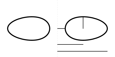
The topology of the horizon is $S^{1}\times S^{2}$, but metrically the geometry is not a simple product of an $S^{1}$ and a round $S^{2}$. Fig. 3 gives an idea of how much rings with the same mass can vary in shape. In this subsection we study in detail the shape of black rings, and we introduce measures for the radii that characterize the $S^{1}$ and $S^{2}$ of the horizon.

Figure 3: Black ring visuals. The azimuthal angle of the $S^{2}$ is suppressed. The plot shows the isometric embedding of the $S^{2}$ cross section (see fig. 4) with the size of the $S^{1}$ estimated as the inner radius of the horizon. All three rings shown have the same mass, and the black rings with $\nu=0.05$ and $\nu=0.95$ also have the same horizon area.

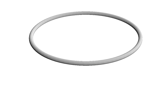
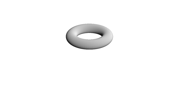
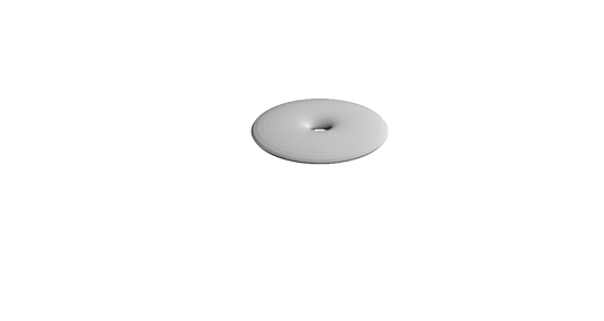
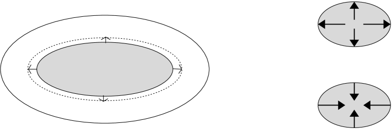
The $S^{2}$ can be highly distorted away from a round sphere, so that measures of the two-sphere radius convey little information about the actual geometry. A useful way of visualizing the shape of the ring, in particular the distortion of the $S^{2}$, is via an isometric embedding of the cross-section of the $S^{2}$ of the black ring horizon (see app. A). This is shown in fig. 4. We show black rings in pairs of equal horizon area: note that $a_{\mathrm{H}}$ in (2.12) is invariant under $\nu\to 1-\nu$.

$${\small~{}~{}~{}~{}~{}\begin{array}[]{r|r|r|r|r|r|r|r}\nu&0.005&0.05&0.2&0.5&0.8&0.95&0.995\\ \hline\cr j&5.04&1.70&1.04&0.92&0.95&0.988&0.999\\ \end{array}}$$

Figure 4: Isometric embedding of the cross-section of the black ring two-sphere for fixed mass $GM=1$. The azimuthal angle is suppressed. The table shows values of the reduced angular momentum $j$ for each $\nu$. The black ring with minimal spin $j^{2}=27/32$ ($\nu=1/2$) is shown in gray. Solutions on the thin black ring branch ($\nu<1/2$) have nearly round two-spheres. The spheres flatten out on the fat black ring branch ($1/2<\nu<1$) as $j\to 1$. A black ring with $\nu=\nu_{0}$ has the same horizon area as one with $\nu=1-\nu_{0}$.

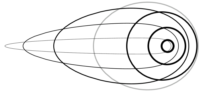
The distortion is particularly important for black rings on the fat ring branch. When $j$ approaches $1$ on the fat ring branch ($\nu\to 1$), the $S^{2}$ flattens out (for fixed mass) and at $j=1$ the horizon disappears and the solution is a singular ring. As $j\to 1$ for the MP black hole, its $S^{3}$ horizon also flattens out. At $j=1$ the (fat) black ring and the MP black hole become the same singular solution.

The radii of the ring circle, $R_{1}$, and two-sphere, $R_{2}$, on the horizon are unambiguously defined only for very thin rings ($\lambda,\nu\to 0$), for which $R_{1}\to R\sqrt{\lambda/\nu}$ and $R_{2}\to R\nu$ [13, 3]. In general the $S^{2}$ is distorted. Furthermore the size of the $S^{1}$ depends non-trivially on the polar angle $x\sim\cos\theta$ of the two-sphere. Several reasonable ways of characterizing $R_{1}$ and $R_{2}$ are possible, see fig. 5 for a sketch, and appendix B for precise definitions. Salient features of their behavior (for black rings of fixed mass) are:

Figure 5: Sketch of a diametrical cross section of the black ring horizon showing some definitions of radii characterizing the black ring horizon: the ‘equator’ radius $R_{2}^{\circ}$ of the $S^{2}$, the inner and outer $S^{1}$ radii, $R_{1}^{\mathrm{inner}}$ and $R_{1}^{\mathrm{outer}}$, and finally $R_{1}^{\circ}$ being the radius of the $S^{1}$ evaluated at the ‘equator’ of the $S^{2}$.

• The inner circle radius of the ring, $R_{1}^{\mathrm{inner}}$, decreases monotonically from the thin branch to the fat branch, and shrinks to zero at the limiting singular solution. The same behavior is shown by $R_{1}^{\circ}$.

• The outer circle radius of the ring, $R_{1}^{\mathrm{outer}}$, decreases along the thin branch until, close to the cusp between branches, it begins to grow. It then increases monotonically to diverge at the limiting singular solution.

Finally, we also note that the rotational velocity of the black ring results in relativistic Lorentz effects. For instance, in the limit of a black string there is a boost factor $\sqrt{\lambda/\nu}$ between the lengths measured at the horizon and the lengths measured at a large transverse distance [12, 13, 3]. We discuss in appendix B how to account for this effect for generic rings. Defining a boost velocity $v$ is mostly sensible for black rings in the thin branch, and the most important result is that in this branch $v$ always remains moderate and not too far from its value at infinite radius, $v\to 1/\sqrt{2}$.

3 Off-shell Probes of Radial Equilibrium

In order to better understand the conditions for equilibrium in a system it is often useful to study the effect of introducing external forces, i.e., probing the system off-shell. By taking it away from equilibrium one can obtain information about the potential that the equilibrium configuration extremizes.

In the case of black rings it is very easy to study the effect of an external radial force that preserves all the Killing symmetries of the system but which deforms the radius of the black ring away from its value at equilibrium. Simply drop the equilibrium condition (2.4), while still preserving (2.3) for asymptotic flatness. Then $\lambda$ is regarded as a parameter independent of $\nu$. In general, this creates a conical defect $\delta$ in the disk inside the ring. This ‘conical membrane’ creates a tension $\tau$ acting per unit length of the black ring circle,

$$\tau=\frac{3}{16\pi G}\;\delta=\frac{3}{8G}\left(1-\frac{1+\nu}{1-\nu}\sqrt{\frac{1-\lambda}{1+\lambda}}\right)\,,$$ (3.1)

which we can view as the force that keeps the off-balance system in a stationary configuration. The normalization factor in the definition of $\tau$ will be justified below. Absence of the conical membrane, $\tau=0$, is equivalent to the equilibrium condition (2.4).

We regard the tension as a function of the $S^{1}$ radius, $\tau(R_{1})$. Given a black ring, we take it out of equilibrium by having $R_{1}=R_{1}^{\mathrm{equil}}+\Delta R_{1}$ (fig. 6). There is obviously an ambiguity in the choice of $S^{1}$ radius $R_{1}$. We will find, however, that for reasonable choices of $R_{1}$ the final results are robust. For visualization purposes it is convenient to plot the radial potential

$$V(R_{1})=-\int^{R_{1}}\tau(R^{\prime}_{1})\,dR^{\prime}_{1}\,,$$ (3.2)

although we are only interested in its value around the equilibrium points ($V^{\prime}=\tau=0$).

Perturbing away from equilibrium, if we find

$$V^{\prime\prime}=-\frac{d\tau}{dR_{1}}\Big{|}_{\mathrm{equil}}>0\,,$$ (3.3)

(negative $\tau$ is pressure) then we infer that the equilibrium is stable: in order to keep the ring static at a larger radius $R_{1}^{\mathrm{equil}}+dR_{1}$, an outward-pushing pressure has to be applied, indicating that the ring wants to return to its original position.

Conversely,

$$V^{\prime\prime}=-\frac{d\tau}{dR_{1}}\Big{|}_{\mathrm{equil}}<0\,$$ (3.4)

is interpreted as the appearance of an inward-pulling tension needed to prevent the runaway increase of the ring radius away from equilibrium, i.e., instability.

Figure 6: Deform the ring away from equilibrium by increasing its (inner) radius, $\Delta R_{1}>0$. The backreaction creates a conical-defect membrane (gray disk) inside the ring. A stable ring tends to return to its original equilibrium radius, hence membrane pressure ($\tau<0$) is needed to keep it static at $R_{1}^{\mathrm{equil}}+\Delta R_{1}$. Instead, membrane tension ($\tau>0$) is required to halt the runaway increase of $R_{1}$ away from equilibrium: an unstable configuration.

Before proceeding to the more general analysis, we study the instructive regime of very thin rings, $\lambda,\nu\ll 1$, since in this limit we recover a Newtonian result for the equilibrium condition.

3.1 Mechanics of thin black rings

When $\lambda,\nu$ are very small we can approximate

$$M\simeq\frac{3\pi}{4G}R^{2}\lambda\,,\quad\Omega\simeq\frac{1}{R}\sqrt{1-\frac{\nu}{\lambda}}\,,\quad\tau\simeq\frac{3}{8G}(\lambda-2\nu)\,,\quad R_{1}\simeq R\sqrt{\frac{\lambda}{\nu}}\,.$$ (3.5)

In this limit there is no ambiguity in the definition of $R_{1}$. Eliminating $\lambda,\nu,R$ from these four equations, thus leaving only physical magnitudes, we find

$$2\pi R_{1}\tau=-\frac{M}{R_{1}}+M\Omega^{2}R_{1}\,.$$ (3.6)

This equation has a neat interpretation. First observe that since $\tau$ is the force that acts at each point along the circle of the ring, the total force acting on it is

$$F=2\pi R_{1}\tau\,.$$ (3.7)

Next, $M/2\pi R_{1}$ is the energy per unit length of the ring, so it is natural to define a string tension

$$\mathcal{T}=\frac{M}{2\pi R_{1}}\,.$$ (3.8)

(As a cautionary note, recall that tension equals energy per unit length only when there is boost-invariance along the string, which is not the case here). Finally, the last term $M\Omega^{2}R_{1}$ is obviously a centrifugal force. The equation (3.6)

$$F=-2\pi\mathcal{T}+M\Omega^{2}R_{1}\,$$ (3.9)

is then exactly the Newtonian result for the equilibrium of a rotating circular string of tension $\mathcal{T}$, total mass $M$, radius $R_{1}$ and angular velocity $\Omega$, under an external centripetal force $F$.

The condition for equilibrium in the absence of the external force fixes

$$\mathcal{T}=\frac{M\Omega^{2}R_{1}}{2\pi}\,.$$ (3.10)

Hence at equilibrium,

$$\Omega R_{1}=1\,,$$ (3.11)

which was observed early on [2].

Notice that the gravitational self-attraction of the ring is absent in (3.9). This force is proportional to $GM^{2}$ and therefore appears only if we expand to $O(\lambda^{2})$. So gravitational forces are only a subleading effect in the balance of very thin black rings. An important consequence of this is the plausibility of the existence of black rings in higher dimensions. The tension and centrifugal forces, being confined to the plane of rotation where the ring lies, are independent of the total number of dimensions — unlike the gravitational force, which is strongly dimension-dependent but negligible for very thin black rings. So we expect the existence of equilibrium configurations of thin rotating black rings in any dimension $D>5$.

A simple argument, based on the phase diagram of fig. 1, suggests that thin black rings should be radially stable. Consider, for fixed total mass and angular momentum, a slight increase in the radius $R_{1}$ away from the equilibrium value. For stationary equilibrium solutions, $j$ increases as the ring radius grows larger, so a ring at larger radius and the same mass requires larger angular momentum to balance itself. Therefore, the radially perturbed solution has less angular momentum than required for balancing the tension, and it would tend to be pulled back to equilibrium. I.e., the thin black ring should be radially stable. This is also the expectation from the Newtonian balance of forces.

3.2 Radial stability

We now apply the method of off-shell radial perturbations to study the stability of black rings, thin as well as fat.

Let us discuss first the practical implementation. First of all, we have to choose a measure for the circle radius. It seems appropriate to consider the inner ring radius $R_{1}^{\mathrm{inner}}=R_{1}^{x=1}$, since we intend to study whether the inner hole of the ring tends to open up or close in as we vary its radius. So we will choose (see (B.4))

$$R_{1}=R^{\mathrm{inner}}_{1}=R\sqrt{\frac{\lambda}{\nu}}\,.$$ (3.12)

As it turns out, qualitatively the results do not depend on the choice of $R_{1}$ as long as this radius behaves monotonically as we move from the thin to the fat ring branch (as is the case for $R^{\mathrm{inner}}_{1}$ and also for $R_{1}^{\circ}$).

We must also specify which quantities we should keep fixed while we take the ring out of equilibrium. These should be quantities that we regard as intrinsic to the black ring as a physical object. It seems natural to keep $J$ fixed: recall that, in a microscopic interpretation with quantized parameters, $J$ measures the number of units of momentum along the direction of the ring. One might also want to keep $M$ fixed. This is slightly tricky since the ADM mass $M$ measured at infinity receives a contribution from the conical disk membrane that is present away from equilibrium. A different possibility is to keep the horizon area fixed. This sounds sensible, since the area, i.e., entropy, is a measure of the number of ring microstates. Keeping it fixed amounts to an adiabatic change.

The adiabatic variation of the radius seems to be the most sensible choice, however, it is just as easy to study both possibilities, i.e., keeping fixed either area and spin, or mass and spin, and so we consider both in the following. Happily, our conclusions turn out not to depend on the choice.

If we vary the solution parameters $R$, $\lambda$ and $\nu$ in such a way that $J$ and ${\cal A}_{H}$, or $J$ and $M$, remain fixed, then there is only one independent variation parameter, say $\nu$. It is again convenient to work with reduced quantities, and to fix the scale of the black rings by fixing one physical magnitude. Since in any case we want to keep $J$ fixed, we introduce a reduced radius

$$r=\frac{R_{1}}{J^{1/3}}\,.$$ (3.13)

If we want to keep $J$ and $M$ fixed then the parameter to use is the reduced spin $j$ introduced in (2.11). Keeping it fixed, $dj=0$, yields

$$\left(\frac{d\lambda}{d\nu}\right)_{M,J}=-\frac{\partial j/\partial\nu}{\partial j/\partial\lambda}=\frac{1-\nu^{2}}{\nu(1+\nu^{2})^{2}}\,.$$ (3.14)

Since we are interested in perturbations around equilibrium configurations, we evaluate the derivatives at equilibrium, $\lambda=\lambda_{c}$ as given in (2.4).

For the purpose of keeping $J$ and ${\cal A}_{H}$ fixed we introduce a second reduced area,

$$\hat{a}_{H}=\frac{{\cal A}_{H}}{J}\,,$$ (3.15)

so that

$$\left(\frac{d\lambda}{d\nu}\right)_{{\cal A}_{H},J}=-\frac{\partial\hat{a}_{H}/\partial\nu}{\partial\hat{a}_{H}/\partial\lambda}=\frac{2(2-\nu)(1-\nu)}{(1+\nu^{2})^{2}}\,,$$ (3.16)

again evaluated at equilibrium.

We can now use these results to compute

$$\left(\frac{d\tau}{dr}\right)_{\ast,J}=\frac{\left(\frac{d\tau}{d\nu}\right)_{\ast,J}}{\left(\frac{dr}{d\nu}\right)_{\ast,J}}=\frac{\partial_{\nu}\tau+\left(\frac{d\lambda}{d\nu}\right)_{\ast,J}\partial_{\lambda}\tau}{\partial_{\nu}r+\left(\frac{d\lambda}{d\nu}\right)_{\ast,J}\partial_{\lambda}r}\,,$$ (3.17)

(with $\ast$ being $M$ or ${\cal A}_{H}$) whose sign will give us, according to the above discussion, the radial stability properties of the black ring.

To see what the sign is, first note that the numerator in (3.17),

$$\left(\frac{d\tau}{d\nu}\right)_{M,J}=\frac{3}{8G}\frac{1-2\nu}{\nu(1-\nu^{2})}\,,$$ (3.18)

or

$$\left(\frac{d\tau}{d\nu}\right)_{{\cal A}_{H},J}=\frac{3}{4G}\frac{1-2\nu}{(1-\nu)(1+\nu)^{2}}\,,$$ (3.19)

in both cases changes sign at $\nu=1/2$ (and only there), which corresponds to the minimally spinning ring at the cusp where the two branches meet.

Next, the denominator in (3.17),

$$\left(\frac{dr}{d\nu}\right)_{M,J}=-\frac{r}{2\nu(1-\nu)}\,,$$ (3.20)

or

$$\left(\frac{dr}{d\nu}\right)_{{\cal A}_{H},J}=-r\frac{1+5\nu-\nu^{2}+\nu^{3}}{3\nu(1-\nu^{2})(1+\nu)}\,,$$ (3.21)

is in both cases negative over the entire parameter range $0\leq\nu<1$.

So for this family of radial perturbations we conclude that

• $\displaystyle\left(-\frac{d\tau}{dr}\right)_{\ast,J}>0$ for $0\leq\nu<1/2$: thin black rings are radially stable.

• $\displaystyle\left(-\frac{d\tau}{dr}\right)_{\ast,J}<0$ for $1/2<\nu<1$: fat black rings are radially unstable.

The conclusion is independent of whether we fix $\ast=M$ or $\ast={\cal A}_{H}$.

Figure 7: Radial potential $V(r)$, for fixed values of the mass and the spin, i.e., for fixed $j$. Fat black rings correspond to unstable equilibrium at local maxima of the potential, and thin black rings to stable local minima. Observe that, in agreement with the phase diagram of fig. 1, the two branches exist when $\sqrt{27/32}<j<1$, and they merge at $j=\sqrt{27/32}$. When $j^{2}>1$ there is a minimum value of the radius for given $M,J$, hence the abrupt termination of the corresponding curves.

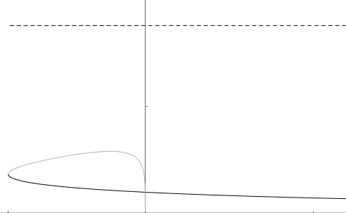
Figure 7 shows radial potentials for representative values of constant $j$. When $\sqrt{27/32}<j<1$, the potential has a local minimum corresponding to the (radially) stable thin black ring, and a local maximum at a smaller value of $r$ corresponding to the unstable fat black ring. When $j=\sqrt{27/32}$ the potential has an inflection point, so the black ring with minimal spin $j$ will also be unstable to radial perturbations. As $j\to 1$, the local maximum of the fat black ring goes to $\infty$, and disappears at $j=1$. Thus for $j\geq 1$, only the local minimum exists corresponding to a radially stable thin black ring with large angular momentum.

The potentials for fixed spin and area are qualitatively similar, with fat black rings sitting at maxima of the potential higher than the minima for thin black rings. Note that the difference in the potential is consistent with the fact that, for fixed spin and area, thin black rings have smaller mass than fat ones.

The shape of the potential suggests that fat black rings can either collapse into a MP black hole, or expand into a thin black ring. If the mass and spin are conserved during the evolution, both possibilities are allowed by the area law. Whether the corresponding MP black hole and thin black ring can themselves be the stable endpoint of the evolution under a generic perturbation is an open issue. A possibility suggested by the phase diagram, fig. 1, is that the final state is the solution that maximizes entropy globally. However, the classical dynamical evolution needs not conform to this expectation. Thin black rings very close to the cusp may be metastable configurations.

As for the minimally spinning ring, the only plausible evolution, also suggested by the shape of the potential, is the collapse into a MP black hole. This is also consistent with the instability found in [6], which we will rederive in sec. 5 below.

The existence of a classical instability for fat black rings, and the change of stability exactly at the cusp at $j=\sqrt{27/32}$, is in agreement with the results of [8]. We discuss this in more detail next.

3.3 Comparison to the ‘turning-point’ method

We have found that the radial stability of the black ring changes at the minimally spinning ring at the cusp at $\nu=1/2$. On this configuration, the radial perturbation can be said to have a zero-mode at linearized level. This feature could in fact have been anticipated without any calculations. To see this, let us discuss the perturbations with $M$ and $J$ fixed — the case with ${\cal A}_{H}$ and $J$ fixed will easily be seen to share the same features.

The configurations of black rings that we are studying correspond to points in the plane $(\nu,\lambda)$, with $\nu,\lambda\in[0,1]$. Equilibrium configurations lie on the curve $\lambda=\lambda_{c}(\nu)$ in eq. (2.4). In our analysis above, we move off-shell away from this curve to a point $(\nu+d\nu,\lambda_{c}+d\lambda)$ in such a way that $j$ remains fixed, $dj=0$. This determines the directional derivative $(d\lambda/d\nu)_{M,J}$, eq. (3.14), along which we move away from the equilibrium curve.

Now consider instead that we move along the on-shell, equilibrium curve. Then $j$ reaches a minimum at the cusp, so $(dj)_{\mathrm{equil}}=0$ at $\nu=1/2$. This means that, at the cusp, the radial deformation with fixed $j$ does not take the ring off-shell but instead moves it to another, infinitesimally nearby, equilibrium solution. So at $\nu=1/2$, $(d\lambda/d\nu)_{M,J}=d\lambda_{c}/d\nu$, i.e., we move tangentially to the equilibrium curve and not away from it, at least at linear order. Hence, there is a linearized marginal (zero-mode) deformation at the cusp. The same argument applies to variations with fixed ${\cal A}_{H}$ and $J$, since $\hat{a}_{H}$ in (3.15) also has an extremum at $\nu=1/2$.

This kind of reasoning is closely related to a previous analysis of black ring stability by Arcioni and Lozano-Tellechea in ref. [8]. It is illuminating to discuss in more detail the connections, and differences, between their approach and ours.

The analysis of ref. [8] uses rather generic arguments based on the ‘Poincaré (or ‘turning-point’) method’. This method only requires qualitative knowledge of the equilibrium curve in the phase diagram. This curve corresponds to extrema of some thermodynamic function, say the entropy in the microcanonical ensemble. By consideration of the possibility of perturbations away from equilibrium, one can conclude that the presence of ‘turning-points’ along the equilibrium curve implies the existence of (at least) one zero mode for some kind of perturbation. The argument is, in fact, exactly the same as we have just given above, only with the difference that we have provided an explicit kind of perturbations away from equilibrium, namely, those that occur when we vary $\lambda$ and $\nu$ independently. The analysis of [8] is more general than ours in that it does not need to specify the form of the perturbation (note that the argument we have given above does not actually use this information either, but is based exclusively on the fact that $j$ reaches a minimum along the equilibrium curve), but then it is more abstract since it does not allow to identify the nature of the instability. In our approach, we have not only specified a particular kind of off-equilibrium deformations, but also identified them as radial deformations. This is made particularly precise from (3.20), which implies that increasing $\nu$ with fixed $M$ and $J$ always results in decreasing $R_{1}$. Hence we can claim that we are perturbing the system by varying the (inner) radius of the ring.

Another difference between our approach and that of [8] concerns the way in which the direction of the change from stability to instability at the turning point is determined. Our arguments can be rephrased as follows. On the plane $(\lambda,\nu)$, on one side of the equilibrium curve $\tau$ is negative, and positive on the other side. So as we deform the ring away from equilibrium, the sign of $d\tau$ will depend on which of the two regions of the plane we are moving into. This direction is given by $(d\lambda/d\nu)_{M,J}$, which can be written as

$$\left(\frac{d\lambda}{d\nu}\right)_{M,J}=\frac{1}{2\nu}\;\lambda_{c}^{\prime}(\nu)\,.$$ (3.22)

We see that for $0<\nu<1/2$ this directional derivative is steeper than the slope of the tangent of the equilibrium curve $\lambda=\lambda_{c}(\nu)$, and therefore the directional derivative takes us to a point above the curve $\lambda_{c}$, where $\tau$ is negative. For $1/2<\nu<1$, the tangent of the equilibrium curve is steeper than the direction of the perturbation and therefore the latter takes us to the $\tau>0$ region below the equilibrium curve. Thus stability does change exactly at $\nu=1/2$ (and only there), where it is, to linear order, indifferent. To determine now which side of the curve is stable and which unstable, it only remains to correlate these directional derivatives to radial variations, using (3.20), and interpret $d\tau/dr$ as we have done above. Note that our analysis does require explicit knowledge of derivatives of $V(r)$ in directions away from the equilibrium curve, and hence of properties of the off-shell configurations.

The reasoning in [8], however, cannot use this off-shell information since the nature of the perturbation away from equilibrium remains unspecified. Instead, they (essentially) use the fact that if we move away from the turning point into the thin black ring branch, the entropy is larger than if we move into the fat branch. By continuity, the former corresponds to local maxima of the entropy (hence stable) and the latter to local minima (hence unstable).

Crucially, observe that the criteria for stability are actually different in the two approaches. In ref. [8] equilibrium configurations are regarded as maxima or minima of a microcanonical potential, i.e., the entropy. Our criterion, instead, determines equilibrium and stability using the (off-shell) radial potential $V(r)$. It is satisfying that these two approaches, one thermodynamical, the other mechanical, consistently yield the same results.

In conclusion, our analysis of radial stability confirms and gives a different, more mechanical perspective on the approach of [8]. Furthermore, it identifies the nature of the instability of the fat ring branch as due to radial perturbations.

4 Gregory-Laflamme Instability and Fragmentation

4.1 Gregory-Laflamme instability in black rings

A static compactified black string $S^{2}\times S^{1}$ suffers from a long-wavelength Gregory-Laflamme instability [14, 15] if the size the two-sphere is small compared with the size of the circle. Introducing the ratio of the radii $k=R_{2}/R_{1}$, the critical value is $k_{\mathrm{GL}}\approx 0.88$, so that for $k\leq k_{\mathrm{GL}}$ the black string is unstable.

We compare the sizes of the horizon $S^{2}$ and $S^{1}$ for the black rings. For large angular momenta $j$ (small $\nu$) the ratio of the $S^{2}$ and $S^{1}$ radii is small, since $R_{2}\sim\nu R$ while $R_{1}\sim\sqrt{2}R$. Hence we expect that black rings are unstable, at least in the thin ring regime, to a Gregory-Laflamme type perturbation. With the various radii defined in the previous section, we can estimate $k$ as a function of the ‘shape parameter’ $\nu$. However, we stress that this will only give a rough estimate. The distortion of the horizon makes the black ring different from the black string and we cannot expect to trust the results for general $\nu$. Based on the results of section 2.2, we would certainly not trust an estimate for fitting a black string Gregory-Laflamme mode on a black ring for $\nu$ beyond $\nu\sim 0.5$, i.e., we do not trust the estimates for fat black rings.

Since the black ring has angular momentum, we must correct for the effect of the velocity. Hovdebo and Myers [11] have shown that for a boosted black string the threshold wavelength can be computed from the static mode by simply including a relativistic contraction; the result is

$$k_{\mathrm{GL}}(v)=\frac{1}{\sqrt{1-v^{2}}}k_{\mathrm{GL}}(0)\,,$$ (4.1)

where $v=|\tanh\beta|$ is the velocity of the black string with boost parameter $\beta$. The boost increases the threshold, making ‘more’ black strings unstable.

Taking the velocity correction into account, we compare for black rings the ratio of $R_{2}/R_{1}$ at given $j$ to the appropriate threshold $k_{\mathrm{GL}}(v)$. We choose the radii measured at the ‘equator’ of the $S^{2}$ (eq. (B.1)), and we use eq. (B.8) to calculate the velocity $v$ (the results for thin black rings are very similar for all other choices of $R_{1}$, $R_{2}$). The practical implementation is most easily done by comparing

$$k_{\mathrm{BR}}\equiv\frac{R_{2}}{R_{1}}\sqrt{1-v^{2}}$$ (4.2)

with $\sqrt{1-v^{2}}\,k_{\mathrm{GL}}(v)\approx 0.88$. Figure 8 shows (4.2) plotted versus $j$. Thin black rings have $k_{\mathrm{BR}}$ smaller by a factor of three or more than the GL threshold $k_{\mathrm{GL}}(0)\simeq 0.88$, and hence they are expected to be unstable.

Figure 8: The ratio $k_{\mathrm{BR}}=\sqrt{1-v^{2}}R_{2}/R_{1}$ versus $j$ for black rings (solid curve) is always well below the Gregory-Laflamme threshold $k_{\mathrm{GL}}\simeq 0.88$ (dashed line), so we expect black rings to be unstable to GL-type modes. Here we use $R_{1}^{\circ}$ and $R_{2}^{\circ}$ for the radius of the $S^{1}$ and $S^{2}$. The plot includes the results for the fat black ring branch (gray), although we do not trust the results in this range.

Strikingly, there is always a very wide margin to accommodate unstable modes. This, together with our analysis of the shape of black rings (fig. 4), strongly suggests that the instability could extend down to values of $j$ very close to its minimum, hence covering most, if not all, of the branch of thin black rings.

4.2 Fragmentation into black holes

If the thin black rings are unstable to Gregory-Laflamme instabilities, then what is the endpoint of the decay? The answer hinges on the unresolved issue of the fate of the black string instability [16, 17, 18, 19]. For black rings, there is the additional effect that the growing inhomogeneities will rotate with the ring, causing a varying quadrupole moment and hence gravitational radiation. However, the timescales for the evolution of the GL instability of thin strings are very short: the inverse frequency of a typical GL unstable mode is of the order of

$$T_{GL}\sim\frac{GM}{R}\,$$ (4.3)

(which seems to remain valid at least insofar as the non-linear evolution has been followed [17]). On the other hand, gravitational radiation is a notoriously inefficient process. We can estimate the rate at which the black ring will lose energy through gravitational radiation by using a rough adaptation to five dimensions of the results from the quadrupole formula in [20] (sec. 36.2) . The timescale for a system to radiate a fraction of its mass is

$$T_{gw}\sim\Omega^{-1}L_{internal}^{-1}$$ (4.4)

where the black ring rotation velocity is $\Omega\sim R^{-1}$ and the dimensionless $L_{internal}$ characterizes the radiating power and can be estimated to be $\sim GM/R^{2}$. Hence

$$T_{gw}\sim\frac{R^{3}}{GM}\,.$$ (4.5)

Since $\sqrt{GM}\ll R$ for thin rings,

$$\frac{T_{GL}}{T_{gw}}\sim\frac{(GM)^{2}}{R^{4}}\ll 1\,,$$ (4.6)

so the effects of gravitational radiation take too long to become noticeable and hence are negligible — unless the black string enters a regime where the evolution of the instability dramatically slows down. Although some slowing-down is observed in the non-linear regime [17], there is no evidence that it will prevent the simplest possibility, i.e., that the black string continues to pinch down to Planck-scale necks in a finite time of order $T_{GL}$ (measured by late asymptotic observers), at which point, through quantum gravity effects, it fragments into black holes of spherical topology.

For the black ring, this implies that it will fragment into a number of black holes flying apart. The simplest way to relate this fragmentation to the GL instability follows the observation in [14, 15] that the unstable regime roughly coincides with the range of parameters where the entropy of split black holes is higher than that of the original black string. A similar argument was used in [7] to argue that higher-dimensional ultraspinning black holes may be unstable. In this section, proceeding along the same lines, we argue that fragmentation of the black ring is entropically possible and so indicates that a GL-like instability may exist for black rings.

The set up for the calculation is actually the same whether the initial black hole is a black ring or a Myers-Perry black hole. We consider as the initial state a black hole with mass $M$ and angular momentum $J$. The final state consists of $n$ black holes, each of mass $m$, infinitely far away from each other and moving in various directions, so that the total momentum is zero and the total angular momentum is $J$. We take the final black holes to be non-spinning, since this maximizes the area of the black holes.

Suppose the splitting occurs with an impact parameter ${\cal R}$. Then, in the center of mass frame, the magnitude of momentum of each of the final black holes is $J/(n{\cal R})$. Assuming, as is usual in these crude calculations, that no energy is lost to radiation in the process of the split-up, we have

$$M=n\sqrt{m^{2}+\frac{J^{2}}{n^{2}{\cal R}^{2}}}\,.$$ (4.7)

Solving for $m$ gives

$$m=\frac{1}{n}\sqrt{M^{2}-\frac{J^{2}}{{\cal R}^{2}}}\,.$$

The total area of the final state black holes is

$$\mathcal{A}_{\mathrm{split}}=2\pi^{2}\,n\,\left(\frac{8G}{3\pi}\,m\right)^{3/2}\,,$$ (4.8)

and so in terms of the dimensionless horizon area we find

$$a_{\mathrm{split}}=\frac{3}{16}\sqrt{\frac{3}{\pi}}\frac{\mathcal{A}_{\mathrm{split}}}{(GM)^{3/2}}=\frac{2\sqrt{2}}{\sqrt{n}}\left(1-\frac{J^{2}}{M^{2}\mathcal{R}^{2}}\right)^{3/4}\,.$$ (4.9)

The fragmentation of a $D$-dimensional highly spinning Myers-Perry black hole as the initial state was considered in [7]. For $D=5$, if for simplicity, we take $\mathcal{R}$ to be equal to the rotation parameter $a=3J/2M$, then the configuration of $n$ fragmented black holes dominates entropically for $j^{2}>1-5\sqrt{5}/(27n)$. For example, for $n=2$, the split two black hole system has $a_{\mathrm{split}}\approx 1.29$ and this is higher than the Myers-Perry black hole entropy when $j>0.89$ (compare with $a_{\mathrm{H}}^{\mathrm{MP}}$ vs. $j$ in figure 1). Note that all black rings have $a_{\mathrm{H}}\leq 1$. Although our approximations are rather crude and these numerical values are therefore not too reliable, the estimates suggest that for $j$ close to its maximum value, the Myers-Perry black hole becomes unstable, and rather than decaying to a black ring, it could fragment into two non-spinning black holes flying apart.

We now take as the initial state a balanced black ring parameterized by $\nu$ and $R$. It is natural to take the splitting radius (impact parameter) $\mathcal{R}$ to be close to the radius of the $S^{1}$ of the black ring. As discussed in section 2.2 and appendix B, this radius depends on $x$, and using $\mathcal{R}=R_{1}^{x}$ (eq. (B.4)) we find that the total horizon area (4.9) of the final state of $n$ black holes is

$$a_{\mathrm{split}}=\frac{2\sqrt{2}}{3\sqrt{3n}}\left(\frac{8-\nu\left(\nu^{2}+\nu+2x(\nu+1)+10\right)}{1-\nu}\right)^{3/4}\,.$$ (4.10)

Presumably, we can only apply this approach for thin black rings ($0<\nu<1/2$), where the horizon distortion is small and the results do not depend much on the choice of $x$ for the radius $R_{1}^{x}$.

Comparing $a_{\mathrm{split}}$ with the reduced area of the black ring $a_{\mathrm{H}}^{\mathrm{BR}}$ of (2.12), we find that fragmentation is always entropically possible. This is in agreement with what we have found from fitting GL modes inside a thin ring. The agreement between both models is in fact fairly good, since there is a nice correlation between the estimate that each of the models gives for the maximum number $n$ of black holes that a given black ring can split into. Taking the splitting radius to be $\mathcal{R}=R_{1}^{\circ}$, the maximum number $n_{\mathrm{split}}$ of black holes which a black ring can fragment into while increasing the entropy in the process is

$$n_{\mathrm{split}}=\left\lfloor\left(\frac{a_{\mathrm{split}}(x=x_{\circ},n=1)}{a_{\mathrm{H}}^{\mathrm{ring}}}\right)^{2}\right\rfloor\,,$$ (4.11)

where $a_{\mathrm{H}}^{\mathrm{ring}}$ is computed using (2.10) and (2.11). This can be compared to the maximum number of Gregory-Laflamme threshold modes $n_{\mathrm{GL}}$ that can be fit on the black ring

$$n_{\mathrm{GL}}=\left\lfloor\frac{R^{\circ}_{1}}{R^{\circ}_{2}}\frac{0.88}{\sqrt{1-v^{2}}}\right\rfloor\,.$$ (4.12)

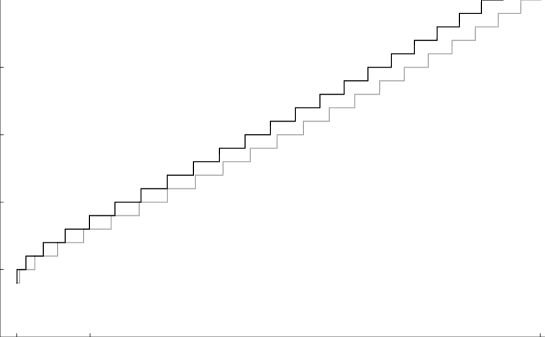
Figure 9 exhibits $n_{\mathrm{GL}}$ and $n_{\mathrm{split}}$ as functions of $j$ for thin black rings ($0<\nu<1/2$), and shows that they are fairly well correlated. The correlation is in fact not wholly unexpected, given that the fragmentation model for black strings already gives a good estimate for the wavelength of the threshold GL mode, and that, as we have seen, thin black rings are well approximated as black strings of finite length.

Figure 9: We see a strong correlation in the maximum number of black holes that a black ring can split into, as a function of $j$, estimated in the two models described in the text: $n_{\mathrm{split}}$ in the fragmentation model (gray) and $n_{\mathrm{GL}}$ (black) in the GL-instability model. The black ring radii are always estimated as $R_{1}^{\circ}$ and $R_{2}^{\circ}$.

It must be noted, though, that neither $n_{\mathrm{GL}}$ nor $n_{\mathrm{split}}$ are the expected number of black holes that the black ring splits into, even within the crudeness of the models involved. Physically, it makes sense to assume that the pinching-off of the black ring will be dominated by the fastest-growing GL modes, i.e., the modes with the largest imaginary frequency. The wavelength of these modes is slightly more than twice the wavelength of the threshold (zero-frequency) mode, so typically this will result in roughly half a number of pinches and therefore half the number of final black holes than $n_{\mathrm{GL}}$ above. In fact, the entropically-favored number of final black holes is not as many of them but instead as few as possible! This minimum number is obviously two. However, typically this requires a GL mode of longer wavelength than the fastest mode. So even if fragmentation into just two black holes may be entropically favored, it will be dynamically suppressed.

So, presumably, the black ring will fragment into a number of black holes dominated roughly by the fastest unstable mode, and this fragmentation will not maximize the final entropy. The split black holes will fly apart and probably will not have the chance to merge into only two black holes to maximize the entropy.

5 Emission/Absorption of Massless Particles

An oft-studied way to test the dynamical stability of black holes is via absorption or emission of small-energy particles [22]. A neutral particle carries away (or dumps in) an energy $\delta E$ and angular momentum $\delta J$, which we assume are small enough to treat it as a test particle moving on a geodesic. An initially stationary black hole is then expected to evolve into an infinitessimally nearby stationary solution with mass $M+\epsilon\,\delta E$ and angular momentum $J+\epsilon\,\delta J$ ($\epsilon=+1$ corresponds to absorption and $\epsilon=-1$ to emission of a particle with energy $\delta E>0$). This evolution is classically possible only if the area of the event horizon does not decrease. Then the first law,

$$\frac{\kappa}{8\pi G}\,\delta\mathcal{A}_{H}=\epsilon(\delta E-\Omega\,\delta J)$$ (5.1)

allows to discriminate between processes that are classically allowed or forbidden.

Consider the absorption of a test particle. It may happen that no infinitessimally nearby, stationary black hole solution is available as a final state (e.g., the solution with those final parameters could have naked singularities), at least not without violating the area law. In this case, the initial black hole cannot smoothly settle into a new stationary state, and the absorption of the particle must be followed by violent backreation — i.e., an instability.

It is often illuminating to also consider the reverse process in which spontaneous emission of test particles takes place — this is of course only a very simplistic model for radiation. Imagine that it is possible for a black hole to ‘emit’ a test particle carrying away $\delta E$ and $\delta J$ in such a way that the horizon area increases after emission. This would be a strong suggestion that the initial black hole is unstable, since it could increase its entropy through spontaneous decay.

When the emitted/absorbed particle is neutral, it is very easy to establish a criterion for these instabilities [7]. On general grounds, one expects a relation between the particle’s energy and spin of the form

$$\alpha\,\delta E=\Omega\,\delta J\,.$$ (5.2)

The dimensionless ‘efficiency coefficient’ $\alpha$ parameterizes the efficiency at which the angular momentum is increased (or decreased) in the process of absorbing/emitting a particle. Note that $\alpha$ is positive (negative) for co-(counter-)rotating geodesics, so that $\delta E>0$ in all cases. Plugging this into (5.1),

$$\frac{\kappa}{8\pi G}\,\delta\mathcal{A}_{H}=\epsilon(1-\alpha)\delta E$$ (5.3)

we see that iff $\alpha\geq 1$, the area law permits spontaneous emission ($\epsilon=-1$), and an instability is expected. Conversely, the absorption ($\epsilon=+1$) of such a particle cannot happen without violating the area law, again signalling the impossibility of smooth classical evolution.

For the purposes of this paper, there are three different kinds of situations where one is motivated to study emission and absorption of test particles:

The first one is as a simple model for an instability of very fastly rotating black objects, as in [7]. An arbitrarily large rotation suggests that the object might spontaneously radiate away angular momentum. This process may also be taken as a simple model for the evolution of the Gregory-Laflamme instability of sec. 4. We studied above the possibility of fragmentation, but another possible evolution is that the inhomogeneities along the ring cause radiation of gravitational waves, which slow down the ring. We may hope to model this crudely as spontaneous emission of massless test particles. Observe that the efficiency parameter $\alpha$ is maximized for a massless particle that tangentially skims the horizon’s edge in corotating sense, and therefore, below we will focus on this case.

The second unstable regime we envisage is in a certain sense the opposite, since we are now interested in minimizing the efficiency parameter. Consider the black ring at the cusp between branches, with $j=j_{min}$. Imagine dropping into it a particle with the effect that $\delta j<0$. Since there are no black rings with $j<j_{min}$, we are in one of the situations considered above, where the system must backreact violently. We will show that there do exist null geodesics with the required properties. Actually, there are many classes of such geodesics (massive particles yield an even more negative $\delta j$), but it will suffice for us to restrict ourselves to null counter-rotating trajectories in the equatorial plane.

Finally, a third possibility is to try to overspin either the MP black hole or the fat black ring beyond their maximal value of $j=1$. This would imply a violation of cosmic censorship.

Thus motivated we study null geodesics in the equatorial plane of a black ring. The geodesic equation is simplified using the conserved energy $\delta E$ and $\delta J$ associated with the Killing vectors $(\partial/\partial t)^{\mu}$ and $(\partial/\partial\psi)^{\mu}$,

$$\delta E=-g_{\mu\nu}(\partial/\partial t)^{\mu}\dot{x}^{\nu}\,,~{}~{}~{}~{}~{}\delta J=\,g_{\mu\nu}(\partial/\partial\psi)^{\mu}\dot{x}^{\nu}\,.$$ (5.4)

The sign in the definition of $\delta J$ is chosen such that positive $\delta J$ gives a co-rotating geodesic and $\delta J$ is negative for a counter-rotating geodesic.

5.1 Black ring geodesics

We study null geodesics in the plane of the ring, restricted to the region outside the ring, $x=-1$. From $g_{\mu\nu}\dot{x}^{\mu}\dot{x}^{\nu}=0$ we obtain

$$\dot{y}^{2}=\xi(y)\equiv A(y,\nu,R)(\delta E)^{2}+2B(y,\nu,R)(\delta J)(\delta E)+D(y,\nu,R)(\delta J)^{2}\,,$$ (5.5)

where

$$A(y,\nu,R) = -g^{tt}\,g^{yy}\Big{|}_{x=-1}=-(1+y)^{2}\frac{(1+y)^{4}C^{2}+(1-\lambda)^{2}G(y)}{R^{2}(1-\lambda)^{2}F(y)}\,,$$

$$B(y,\nu,R) = \frac{2\pi}{\Delta\psi}\,g^{t\psi}\,g^{yy}\Big{|}_{x=-1}=\frac{2\pi}{\Delta\psi}\frac{(1+y)^{5}C}{R^{3}(1-\lambda)^{2}}\,,$$

$$D(y,\nu,R) = -\left(\frac{2\pi}{\Delta\psi}\right)^{2}\,g^{\psi\psi}\,g^{yy}\Big{|}_{x=-1}=-\frac{4\pi^{2}}{\left(\Delta\psi\right)^{2}}\frac{(1+y)^{4}F(y)}{R^{4}(1-\lambda)^{2}}\,.$$

The analysis is done for the equilibrium black rings, so it is here understood that $\lambda=\lambda_{c}$ as given by (2.4). The factors of $\frac{\Delta\psi}{2\pi}$ are required in order to make the angle $\psi$ canonically normalized at infinity.

Finding the efficiency coefficient $\alpha$ is the problem of simultaneously solving $\xi(y)=0$ and $\xi^{\prime}(y)=0$. Making a coordinate transformation $y=y(r)$, eq. (5.5) becomes $\dot{r}^{2}=U(r)$, where $U(r)=\xi(y(r))/(y^{\prime}(r))^{2}$. A solution to the problem $U(r)=0=U^{\prime}(r)$ is also a solution to the original problem, provided that $1/y^{\prime}(r)$ does not vanish for the solution. Now define

$$r=-R\frac{1-\nu}{\nu(1+y)}\,.$$ (5.6)

Asymptotically, $y\to-1$, we have $r\to\infty$, and the normalization is chosen such that $r=R$ at the horizon $y=-1/\nu$. Next set $\delta J=\alpha\,\delta E/\Omega$, with $\Omega$ given in (2.9). We are assuming that the ring is balanced, so that in all expressions $\lambda$ is eliminated using (2.4).

It is now easy to see that $U(r)$ has a maximum at $r=r_{c}$ with

$$r_{c}^{2}=\frac{R^{2}(1+\nu)(1-2\alpha+\nu)^{2}}{2\nu\,(1-\nu)^{2}}\,.$$ (5.7)

Next, $U(r_{c})=0$ reduces to

$$1+3\nu^{2}-2\alpha^{2}(1+\nu)+2\sqrt{2\nu\,(1+\nu)}|1-2\alpha+\nu|=0\,.$$ (5.8)

There are two solutions,

$$\alpha=-\sqrt{\nu}\pm\frac{(1+\sqrt{\nu})^{2}}{\sqrt{2}\sqrt{1+\nu}}\,,$$ (5.9)

corresponding to co-rotating ($+$) and counter-rotating ($-$) geodesics. In both cases, $|\alpha|\to 1/\sqrt{2}$ in the limit $\nu\to 0$.

The analysis for the Myers-Perry black hole with a single angular momentum was done in [7] (for arbitrary dimension), and can also be recovered from our results above by taking the limit to the MP bh as described in [3, 13]. The efficiency coefficient for MP black holes is

$$\alpha=\frac{a}{m}\left(\pm 2\sqrt{m}-a\right)$$ (5.10)

with “$+$” for co-rotating and “$-$” for counter-rotating geodesics.

Figure 10 shows $|\alpha|$ versus $j$ for the black ring and the Myers-Perry black hole for the co-rotating and counter-rotating null geodesics. It is curious that for thin black rings, the efficiency of shedding off angular momentum via emission of null particles decreases with the angular momentum of the ring, contrary to what happens for MP black holes. This is related to the property that, for a thin black ring of fixed mass, the angular velocity decreases with angular momentum (see figure 2).

     

Figure 10: The efficiency parameter $\alpha$ for co-rotating (left) and counter-rotating (right) null geodesics in the equatorial plane plotted versus the angular momentum $j$. For the counter-rotating case, $\alpha$ is negative so the plot actually shows $-\alpha$. The dashed curves shows $\alpha$ for the Myers-Perry black hole, the full curve is $\alpha$ for the black ring.

We consider now the four cases of absorbing/emitting co-(counter-)rotating null particles in the equatorial plane, and the possible associated instabilities mentioned above (the last fourth case is included for completeness):

Absorption of co-rotating null particles: Impossibility of overspinning the MP black hole and fat black ring.

It is clearly possible to spin up a generic Myers-Perry black hole or black ring by throwing in a co-rotating null particle: according to eq. (5.1), this requires $0<\alpha<1$, which holds for both the MP black hole and the black ring. It is easy to check that in both cases the effect is that the reduced angular momentum increases, $\delta j>0$. However, in the singular limit of $j\to 1$ ($\nu\to 1$ for the fat black ring), one finds that $\delta j\to 0$, so cosmic censorship is not violated in the process.

Absorption of counter-rotating null particles: Destabilizing the minimally spinning black ring by slowing it down.

The counter-rotating null geodesics have $\alpha<0$, and hence again $\delta\mathcal{A}_{H}$ will be positive. It is therefore possible to decrease the angular momentum, and hence $j$, of the MP black hole or the black ring by absorption of a null particle. For the black ring with minimal angular momentum, $j=\sqrt{27/32}$, there is no other black ring it can evolve into. We expect it to collapse to a Myers-Perry black hole, which, for that value of $j$, has (much) higher entropy.

Emission of co-rotating null particles: No spontaneous decay by radiation.

The spontaneous emission ($\epsilon=-1$) of a null particle with energy $\delta E$ and $\delta J>0$ requires $\alpha\geq 1$. However, we always have $\alpha\leq 1$ for both the MP black hole and the black ring have, with equality only for the singular solution with $j=1$ (see figure 10). So the Myers-Perry black hole and the black ring are not unstable to the spontaneous emission of null particles carrying away energy and angular momentum.

Emission of counter-rotating null particles: No spontaneous spin-ups.

It is impossible to increase the angular momentum of the black hole by spontaneously radiating away a null particle in the equatorial plane: with $\epsilon=-1$ and $\delta J<0$ (so $\alpha<0$) we always have $\delta\mathcal{A}_{H}<0$.

6 Thermodynamics and Euclidean Black Rings

Fig. 1 can be regarded as a microcanonical phase diagram, where the thermodynamic potential is the entropy $S[M,J]$. It is interesting to study other thermodynamical ensembles, in particular the grand-canonical ensemble where the variables are the temperature $T$ and angular velocity $\Omega$ at the horizon. A previous related study can be found in [21].

A frequently used method derives the grand potential $W[\Omega,T]$ from the saddle-point approximation to the Euclidean black hole partition function, in terms of the action of a real Euclidean regular section of the solution, as $I_{Euc}=W[\Omega,T]/T$ (recall that, without any other boundary terms, the Einstein-Hilbert-Gibbons-Hawking action is extremized at fixed $T$ and $\Omega$). For the black ring, such a real, non-singular Euclidean metric does not seem to exist.

To see this, recall first that for generic spinning black holes the Euclidean rotation $t\to-i\tau$ does not give a real Euclidean metric, due to the presence of off-diagonal time-space metric components. To obtain a real Euclidean solution the angular velocity parameter needs to be analytically continued to imaginary values. In the case of the Kerr or Myers-Perry solutions this is achieved by continuing $a\to ia$. In the parametrization above we would take $0<\lambda<\nu<1$ and $-1/\nu\leq y\leq-1$, and then take the limit to the MP black hole.

If we try to do the same for the black ring, we find that the range of values $0<\lambda<\nu<1$ is incompatible with the balance condition (2.4) and therefore the instanton will possess a naked conical singularity. Instead we may try to maintain the condition (2.4) in order to eliminate the conical singularity, but then change the range of values of $\nu$ to make $C$ purely imaginary so as to obtain a real solution. For real $\nu$ this requires $|\nu|>1$. It is then easy to see that if the instanton is to be Euclidean, real, and asymptotically flat, it will have a naked curvature singularity. So it does not seem possible to construct a non-singular real Euclidean metric from the black ring.

However, the use of complex Euclidean geometries, where only time and not the parameters of the solution is Wick-rotated, was advocated in [23]. These solutions can still yield a real Euclidean action, and the resulting grand potential coincides with the conventional thermodynamics definition

$$W[\Omega,T]=M-TS-\Omega J$$ (6.11)

where the entropy is given by the area law $S=\frac{\mathcal{A}_{H}}{4G}$ and the temperature by the surface gravity $T=\kappa/2\pi$ (see also [21]). Using the Smarr relation $\frac{2}{3}M=TS+\Omega J$,

$$W[\Omega,T]=\frac{M}{3},$$ (6.12)

which is actually valid for both the Myers-Perry black hole and the black ring.

Figure 11: Grand-canonical potential $W[T,\Omega]$ as a function of $T$, for fixed $\Omega$. Black ring is solid curve, MP black hole is dotted curve.

Fig. 11 is a plot of the grand-canonical potential in which we have fixed the scale by fixing $\Omega$, and then vary $T$. I.e., we plot $\Omega^{2}W$ vs. $T/\Omega$. This shows some significant differences with respect to the microcanonical ensemble. There is always one black ring (and only one) and one MP black hole with the same values of $\Omega$ and $T$. Both kinds of solutions exist for all possible values of $\Omega$ and $T$. The global thermodynamic stability in the grand-canonical ensemble is determined by minimizing the potential $W$: the MP black hole always has lower potential than the black ring. So in this ensemble the MP black hole is always thermodynamically favored over the black ring.

Of course it is not unusual that the phase structure and global thermodynamical stability of black holes depend on the ensemble considered, since some ensembles possess conserved charges that others do not. For the system at hand, other ensembles may be studied, which result in curious differences. In the canonical ensemble, the free energy $F[T,J]=M-TS$ exhibits a ‘swallowtail’ structure, but different than the microcanonical one. Fixing $T$, there is a range of $J$ for which there are two MP black holes and only one black ring, i.e., opposite to the microcanonical phase diagram. At small $J$ one of the MP black holes minimizes $F$ and so is preferred, then at a certain value of $J$ we cross the swallowtail and the black ring is preferred, and for large $J$ only the black ring exists. The ‘enthalpy’ $H[M,\Omega]=M-\Omega J$ gives yet a different phase structure. In this case, the solutions exist only in a finite range of parameters, and there are always one MP black hole and one black ring for each value of parameters. But now the enthalpy is always minimized by the black ring, and so in this ensemble the black ring is always preferred.

7 Discussion

We have found evidence that

• Fat black rings are unstable to radial perturbations, while thin black rings are radially stable.

• Most thin black rings also suffer from GL instabilities.

• The minimally spinning ring is unstable.

As discussed in sec. 3.3, the first instability result in this list (although not the nature of the instability) actually follows from general considerations studied in [8]. The possible appearance or disappearance of unstable modes along the curve of equilibrium states comes from the existence of turning points or bifurcations, and the current phase diagram allows us to identify only the cusp as a point where unstable modes appear. It must be noted, though, that it is possible that only axisymmetric modes are accounted for by the Poincaré method [8]. In this case the GL instability would likely be invisible to it, and it can possibly switch off at some value of $j$ along the thin black ring branch. This would allow the existence of absolutely stable thin black rings for moderate values of $j$, perhaps within a range roughly coincident with the range where non-uniqueness happens. Evidently this requires the absence of any unstable modes besides those we have studied. This problem clearly deserves further study.

It does not seem probable that additional neutral black hole solutions with a single connected horizon and as many as three Killing symmetries exist in $D=5$. On the other hand, black hole phases with broken axial symmetry along $\phi$ have been conjectured [24]. They may play a role if the MP black hole actually becomes unstable near $j=1$.

The conclusions above apply to neutral black rings with a single angular momentum. The addition of a second angular momentum along the $S^{2}$ may change the behavior of some of the instabilities we have analyzed. However, doubly-spinning black rings are likely to suffer from superradiant instabilities peculiar to extended black objects with a rotating sphere [25].

It is therefore likely that neutral black rings, with one or two angular momenta, are dynamically unstable to some kind of perturbation over a wide range of parameters. If they are actually unstable for all parameter values, then black rings may be difficult, perhaps impossible, to produce in physical processes. However, does this imply that these black rings are irrelevant as physical objects?

The answer, of course, depends on the relative value between the time scale for the evolution of the instabilities and the time scales of the physical processes considered. Slow instabilities may become essentially negligible for many purposes.

The information we have at the moment about the time scales for instabilities is rather scarce. We have argued in sec. 4.2 that the time scale for the Gregory-Laflamme instability of thin rings is very quick, eq. (4.3), although it could turn into a much slower one, eq. (4.5), if the GL instability of black strings slows down, and possibly halts, as suggested in [16]. The superradiant instabilities of black rings with two angular momenta are expected to be very slow too [25].

As for the time scale for radial instabilities, we do not really know. Naively, the curvature $V^{\prime\prime}$ of the radial potential around the equilibrium point gives the square of the imaginary frequency of the unstable mode. However, it is not quite clear whether the potential (3.2) (even if properly normalized) can be used for this purpose, since the time evolution of the system presumably happens through highly-dynamical geometries that have little to do with the conically-deformed ones that we have studied.

Given the uncertainty about many dynamical aspects of higher-dimensional gravity, one should also be cautious when speculating about the evolution of these instabilities. It seems natural to expect that the radial instabilities of fat black rings follow the evolution suggested by the potential in fig. 7. Less clear is the evolution of the GL instability. The break-up into black holes flying apart gives a simple physical picture. However, it would not be unprecedented in this field if wholly new phenomena were at play.

The inclusion of charges does improve stability: supersymmetric black rings [26] are expected to be stable, and near-supersymmetric ones [27] probably too. There also exist black rings with dipole charges but no conserved charges [13]. We have performed the analysis of radial stability for these dipole rings (see appendix C), and the conclusions are similar to what we have found for neutral rings: when the dipole charge is fixed, in addition to the area and spin, thin rings appear to be radially stable, fat rings unstable. This also applies, in particular, for the extremal dipole rings (which are not supersymmetric) with a regular horizon. One expects that close to the extremal limit the GL instability switches off. So it is very well possible that thin dipole rings close to extremality are dynamically stable.

It might be possible to gain more insight on the dynamics of higher-dimensional black holes using their string theory description. Supersymmetric and near-supersymmetric black holes can be understood as excited D-brane systems in string theory. D-branes are highly dynamical objects that can move and ripple, so from the point of view of string theory it comes as no surprise that black holes are also dynamical objects. Picturing neutral black holes as brane-antibrane systems [28, 29] — the branes and antibranes entering with equal and opposite charges thus leaving no net charge (nor any higher moments of charge) — there are even microscopic indications of phenomena such as the GL instability [29]. String models for black rings with dipole charges have been suggested [13]. In these models, strings (or branes) wind around the circle of the ring. With this in mind it is perhaps noteworthy that at leading order we have found the balance of (thin) black rings to be dominated by a string-like tension rather than a gravitational force. A better understanding of the microscopics of black rings may therefore give valuable hints about their macroscopic dynamics.

Appendix A Isometric Embedding

The idea of isometric embedding is to visualize a curved geometry in flat Euclidean space in a way that preserves the distances. Not all 2d surfaces can be embedded isometrically in 3d euclidean space, but the two-sphere of the black ring can be embedded in $\mathbb{E}^{3}$.

Consider a surface H with metric

$$ds_{\mathrm{H}}^{2}=g_{\theta\theta}\,d\theta^{2}+g_{\phi\phi}\,d\phi^{2}\,,$$ (A.1)

where the metric functions depend on $\theta$ only and $0\leq\theta\leq\pi$. We wish to embed this into a non-physical 3d euclidean space

$$ds^{2}(\mathbb{E}^{3})=dx^{2}+dy^{2}+dz^{2}\,.$$ (A.2)

Let

$$x=f(\theta)\,\cos\phi\,,~{}~{}~{}~{}~{}~{}y=f(\theta)\,\sin\phi\,,~{}~{}~{}~{}~{}~{}z=g(\theta)\,.$$ (A.3)

Then from $ds_{\mathrm{H}}^{2}=ds^{2}(\mathbb{E}^{3})$ we get

$$f=\sqrt{g_{\phi\phi}}\,,~{}~{}~{}~{}~{}~{}~{}{g^{\prime}}^{2}=g_{\theta\theta}-{f^{\prime}}^{2}\,.$$ (A.4)

The necessary condition for the embedding of the surface H into $\mathbb{E}^{3}$ is then that

$$g_{\theta\theta}\geq\left(\partial_{\theta}\sqrt{g_{\phi\phi}}\right)^{2}\,.$$ (A.5)

The embedding condition (A.5) is satisfied for the two-sphere of the black ring horizon. Fig. 4 shows the cross-section of the black ring two-sphere for various values of $j$ ($\nu$) with the mass $GM$ fixed. The figure is produced as a parametric plot of $f(\theta)$ versus $g(\theta)$, suppressing the azimuthal angle $\phi$. Fig. 3 was made using the isometric embedding of the $S^{2}$ cross section of fig. 4, but with the $S^{1}$ fixed to match the inner radius of the $S^{1}$. Thus fig. 3 is simply a cartoon of the black ring geometry.

Appendix B Ring Radii and Rotation Velocity

Since in general the black ring horizon is distorted, the definitions of the radii of the circle and the two-sphere are ambiguous. In the following, we introduce different definitions. For definitions of the $S^{2}$ radii, we shall assume the balancing condition (2.4), but in applications is useful to also define the $S^{1}$ radii for black rings away from mechanical equilibrium.

B.1 Radius of $S^{2}$: $R_{2}$

One possibility is to define the radius $R_{2}^{\circ}$ at the ‘equator’ where the sphere is fattest, namely at

$$x_{\circ}=\frac{-1+\sqrt{1-\nu^{2}}}{\nu}\,,$$ (B.1)

as can be seen from the horizon metric (2.5). This gives the ‘equator radius’ of the $S^{2}$,

$$R_{2}^{\circ}=R\,\sqrt{\frac{2-2\sqrt{1-\nu^{2}}}{1+\nu^{2}}}\,.$$ (B.2)

Another option is to use the area of the $S^{2}$ on the horizon (at constant $t$ and $\psi$) to define the radius as

$$R_{2}^{\mathrm{area}}=\sqrt{\frac{\mathcal{A}_{S^{2}}}{4\pi}}=\left(\frac{1}{2}\frac{\Delta\phi}{2\pi}\int_{-1}^{1}dx\,\sqrt{g_{xx}\,g_{\phi\phi}}\Big{|}_{y=-1/\nu}\right)^{1/2}\ .$$ (B.3)

The definitions $R_{2}^{\circ}$ and $R_{2}^{\mathrm{area}}$ agree well for black rings on the thin ring branch, as can be seen in fig. 12(a). The agreements is expected, since the $S^{2}$ is nearly round for thin black rings (see fig. 4). As $\nu\to 0$ both $R_{2}^{\circ}$ and $R_{2}^{\mathrm{area}}$ tend to the value $R\nu$ equal to the area radius of the $S^{2}$ for the boosted black string.

In the singular limit $\nu\to 1$, both $R_{2}^{\circ}$ and $R_{2}^{\mathrm{area}}$ go to zero. The effect is that the horizon flattens out before finally disappearing for $\nu=1$.

B.2 Radius of $S^{1}$: $R_{1}$

The radius of the circle measured at a given polar angle on the $S^{2}$, specified by $x$, is

$$R_{1}^{x}=\frac{\Delta\psi}{2\pi}\sqrt{g_{\psi\psi}(y=-\nu^{-1},x)}=R\,\sqrt{\frac{\lambda(1+\lambda)}{\nu(1+\lambda x)}}\,.$$ (B.4)

For very thin rings, $\lambda,\nu\to 0$, the $S^{1}$ radius goes to $R\sqrt{\lambda/\nu}$ independently of $x$. We will see below that the factor $\sqrt{\lambda/\nu}$ is a relativistic boost effect.

There are several values of $x$ of particular interest: inside of the ring at $x=1$, on the outside at $x=-1$, or at the $S^{2}$ ‘equator’ at $x=x_{\circ}$. Assuming, for illustration, the condition for equilibrium (2.4) one finds

$$R_{1}^{\mathrm{inner}}=R\,\sqrt{\frac{2}{1+\nu^{2}}}\,,~{}~{}~{}~{}~{}R_{1}^{\mathrm{outer}}=R\,\frac{1+\nu}{1-\nu}\sqrt{\frac{2}{1+\nu^{2}}}\,,~{}~{}~{}~{}~{}R_{1}^{\circ}=R\,\frac{\sqrt{2}\,(1+\nu)}{\sqrt{(1+\nu^{2})\big{(}2\sqrt{1-\nu^{2}}+\nu^{2}-1\big{)}}}\,.$$ (B.5)

Another useful measure for the $R_{1}$ is based on the horizon area $\mathcal{A}_{\mathrm{H}}$:

$$R_{1}^{\mathrm{area}}=\frac{\mathcal{A}_{\mathrm{H}}}{8\pi^{2}(R_{2}^{\circ})^{2}}\,.$$ (B.6)

For $\nu\to 1$, $R_{1}^{\mathrm{inner}}$ and $R_{1}^{\circ}$ go to zero while $R_{1}^{\mathrm{outer}}$ and $R_{1}^{\mathrm{area}}$ diverge: as the black ring approaches the singularity, the hole inside the ring shrinks to zero size while the outer radius goes to infinity.

Figure 12(b) compares for fixed mass the four definitions of the circle radii plotted as functions of the reduced angular momentum $j$. For black rings on the thin ring branch ($\nu<1/2$) the area-radius and $R_{1}^{\circ}$ agree fairly well, especially for large angular momenta. In fact, at large angular momenta one finds that, for fixed mass, the $S^{1}$ radius grows linearly with $j$.

(a) Radii for the $S^{2}$.

(b) Radii for the $S^{1}$.

Figure 12: For fixed mass, $GM=1$, the various definitions of radii of the two-sphere (figure 12(a)) and of the circle (figure 12(b)) are plotted vs. the reduced angular momentum $j$.

We can also define an $S^{2}$ radius $R_{2}^{\mathcal{A}_{\mathrm{H}}}$ based on the total area $\mathcal{A}_{\mathrm{H}}$ of the black ring. Using $R_{1}^{\circ}$ for the radius of the circle to extract $R_{2}^{\mathcal{A}_{\mathrm{H}}}$ from the total area $\mathcal{A}_{\mathrm{H}}$, this definition agrees well with the other two definitions for thin black rings, see figure 12(a).

B.3 Rotation velocity

Since the black ring has angular momentum, it experiences effects of Lorentz contraction. For our purposes in section 4 it is desirable to have a way to account for this effect. This requires making some judicious estimate for the boost velocity $v$ of the black ring.

In the limit of infinite radius the balanced black ring becomes a boosted black string with velocity $v=\sqrt{1-\nu/\lambda}$ [13]. So we require that our definition of $v$ for the black ring reproduces this limit for $\lambda,\nu\to 0$. It is natural to base the definition of $v$ on the angular velocity $\Omega$ of the black ring. Indeed for the boosted black string, $v=\Omega\,R_{1}(\infty)$, where $R_{1}(\infty)$ is the radius of the circle at infinity. For the black ring there is of course no circle at infinity, so we have to base the definition on the radius of the $S^{1}$ of the horizon. Note that for the boosted black string, the radius of the $S^{1}$ of the horizon is $R_{1}(\mathrm{horizon})=R_{1}(\infty)/\sqrt{1-v^{2}}$. Thus motivated we define $v$ for the black ring by

$$v=\Omega R_{1}\sqrt{1-v^{2}}$$ (B.7)

i.e.,

$$v=\frac{\Omega R_{1}}{\sqrt{1+(\Omega R_{1})^{2}}}\,,$$ (B.8)

for some choice $R_{1}$ of the $S^{1}$ radius. If we use $R_{1}=R_{1}^{x}$, then (B.4) gives

$$v=\sqrt{\left(1-\frac{\nu}{\lambda}\right)\frac{1}{1+\nu x}}\,.$$ (B.9)

Note that we recover $v=\sqrt{1-\nu/\lambda}$ as $\lambda,\nu\to 0$.

Appendix C Radial stability of dipole rings

The analysis of radial stability in sec. 3.2 can be extended to black rings with dipoles. The same result is obtained as for neutral rings: fat black rings are radially unstable, thin black rings are radially stable. That the minimally spinning ring separates the two stability regimes follows from a general argument as in sec. 3.3. The general analysis is rather tedious, so for the purpose of illustration here we only provide details for a case of particular significance: dipole rings with extremal (maximal) dipole charge, and with a regular horizon.

These are black ring solutions of non-dilatonic Einstein-Maxwell theory (with, possibly, an additional Chern-Simons term, as required by minimal 5D supergravity) with a dipole $q$ [13]. They can be regarded as intersections of three stacks of M5-branes over a ring, with equal numbers of branes in each stack. In the extremal limit the horizon is degenerate (zero-temperature) but still is non-singular and has finite area.

Fixing the scale, the solutions are characterized by a single dimensionless parameter $\mu$, in terms of which we can express the reduced spin, area, and dipole as [13]

$$j^{2}=\frac{(1+\mu)^{6}(3+\mu^{2})^{2}}{128\mu(1+\mu^{2})^{3}}\,,\quad{a_{H}}=\sqrt{\frac{\mu(1-\mu^{2})^{3}(3+\mu^{2})}{4(1+\mu^{2})^{3}}}\,,\quad{\hat{q}}=\sqrt{\frac{\mu(1-\mu)^{2}}{\pi(1+\mu^{2})}}\,,$$ (C.1)

which are valid for the equilibrium configurations. The spin $j$ reaches a minimum value at the real root of

$$\mu_{c}(3+\mu_{c}+\mu_{c}^{2})=1\,,$$ (C.2)

(i.e., $\mu_{c}\simeq 0.296$) which separates the branches of thin rings, $0\leq\mu<\mu_{c}$, and fat rings $\mu_{c}<\mu<1$.

Following the analysis in sec. 3.2, we now perturb these configurations by varying the inner radius $R_{1}^{\mathrm{inner}}$ away from its equilibrium value. This generates a membrane disk with tension

$$\tau=\frac{3}{8G}\left(1-\sqrt{\frac{1-\lambda}{1+\lambda}}\left(\frac{1+\mu}{1-\mu}\right)^{3/2}\right)$$ (C.3)

where, at equilibrium, $\lambda=\mu(3+\mu^{2})/(1+3\mu^{2})$.

We have to choose whether we keep fixed the spin and the area, or the spin and the dipole. We have checked both cases and found analytically that they yield the same conclusions for radial stability. In particular, if we fix the spin and dipole we find

$$\left(-\frac{d\tau}{dr}\right)_{J,q}=\frac{9}{4G}\frac{1-\mu(3+\mu+\mu^{2})}{\big{(}5+\mu(3+3\mu+\mu^{2})\big{)}r}\,.$$ (C.4)

This is positive, hence stable, for thin rings, and as expected, changes sign precisely at the cusp $\mu=\mu_{c}$, (C.2), rendering fat rings radially unstable.

For the non-extremal case, the calculation of $\left(d\tau/dr\right)_{J,q,\ast}$ with $\ast=M,\mathcal{A}_{H}$, is straightforward, and one gets a polynomial in $\nu$ and $\mu$. The only complication is finding out, for fixed $q$, at which value of $\nu$ is the cusp separating the branches located. We have done this numerically, and checked again that fat rings are radially unstable, with stability changing at the cusp.

Finally, the results can also be extended to dilatonic dipole rings.

References

- [1] S. Chandrasekhar, “The Mathematical Theory Of Black Holes,” Oxford University Press (1983).
- [2] R. Emparan and H. S. Reall, “A rotating black ring in five dimensions,” Phys. Rev. Lett. 88, 101101 (2002) [arXiv:hep-th/0110260].
- [3] R. Emparan and H. S. Reall, “Black Rings,” arXiv:hep-th/0608012.
- [4] R. C. Myers and M. J. Perry, “Black Holes In Higher Dimensional Space-Times,” Annals Phys. 172, 304 (1986).
- [5] H. K. Kunduri, J. Lucietti and H. S. Reall, “Gravitational perturbations of higher dimensional rotating black holes,” arXiv:hep-th/0606076.
- [6] R. Emparan and H. S. Reall, “Essay: The End of Black Hole Uniqueness,” Gen. Rel. Grav. 34, 2057 (2002).
- [7] R. Emparan and R. C. Myers, “Instability of ultra-spinning black holes,” JHEP 0309, 025 (2003) [arXiv:hep-th/0308056].
- [8] G. Arcioni and E. Lozano-Tellechea, “Stability and critical phenomena of black holes and black rings,” Phys. Rev. D 72, 104021 (2005) [arXiv:hep-th/0412118]. G. Arcioni and E. Lozano-Tellechea, “Stability and thermodynamics of black rings,” arXiv:hep-th/0502121.
- [9] M. Nozawa and K. i. Maeda, “Energy extraction from higher dimensional black holes and black rings,” Phys. Rev. D 71, 084028 (2005) [arXiv:hep-th/0502166].
- [10] V. Cardoso, O. J. C. Dias and S. Yoshida, “Perturbations and absorption cross-section of infinite-radius black rings,” Phys. Rev. D 72, 024025 (2005) [arXiv:hep-th/0505209].
- [11] J. L. Hovdebo and R. C. Myers, “Black rings, boosted strings and Gregory-Laflamme,” Phys. Rev. D 73, 084013 (2006) [arXiv:hep-th/0601079].
- [12] H. Elvang and R. Emparan, “Black rings, supertubes, and a stringy resolution of black hole non-uniqueness,” JHEP 0311, 035 (2003) [arXiv:hep-th/0310008].
- [13] R. Emparan, “Rotating circular strings, and infinite non-uniqueness of black rings,” JHEP 0403, 064 (2004) [arXiv:hep-th/0402149].
- [14] R. Gregory and R. Laflamme, “Black strings and p-branes are unstable,” Phys. Rev. Lett. 70, 2837 (1993) [arXiv:hep-th/9301052].
- [15] R. Gregory and R. Laflamme, “The Instability of charged black strings and p-branes,” Nucl. Phys. B 428, 399 (1994) [arXiv:hep-th/9404071].
- [16] G. T. Horowitz and K. Maeda, “Fate of the black string instability,” Phys. Rev. Lett. 87, 131301 (2001) [arXiv:hep-th/0105111].
- [17] M. W. Choptuik, L. Lehner, I. Olabarrieta, R. Petryk, F. Pretorius and H. Villegas, “Towards the final fate of an unstable black string,” Phys. Rev. D 68, 044001 (2003) [arXiv:gr-qc/0304085].
- [18] D. Marolf, “On the fate of black string instabilities: An observation,” Phys. Rev. D 71, 127504 (2005) [arXiv:hep-th/0504045].
- [19] B. Kol, “The phase transition between caged black holes and black strings: A review,” Phys. Rept. 422, 119 (2006) [arXiv:hep-th/0411240]. T. Harmark and N. A. Obers, “Phases of Kaluza-Klein black holes: A brief review,” arXiv:hep-th/0503020.
- [20] C. W. Misner, K. S. Thorne and J. A. Wheeler, “Gravitation,” W. H. Freeman, San Francisco, 1973.
- [21] D. Astefanesei and E. Radu, “Quasilocal formalism and black ring thermodynamics,” Phys. Rev. D 73 (2006) 044014 [arXiv:hep-th/0509144].
- [22] R. M. Wald, “Gedanken experiments to destroy a black hole,” Annals Phys. 82 (1974) 548.
- [23] J. D. Brown, E. A. Martinez and J. W. York, “Complex Kerr-Newman geometry and black hole thermodynamics,” Phys. Rev. Lett. 66 (1991) 2281.
- [24] H. S. Reall, “Higher dimensional black holes and supersymmetry,” Phys. Rev. D 68 (2003) 024024 [arXiv:hep-th/0211290].
- [25] O. J. C. Dias, “Superradiant instability of large radius doubly spinning black rings,” Phys. Rev. D 73, 124035 (2006) [arXiv:hep-th/0602064].
- [26] H. Elvang, R. Emparan, D. Mateos and H. S. Reall, “A supersymmetric black ring,” Phys. Rev. Lett. 93, 211302 (2004) [arXiv:hep-th/0407065].
- [27] H. Elvang, R. Emparan and P. Figueras, “Non-supersymmetric black rings as thermally excited supertubes,” JHEP 0502, 031 (2005) [arXiv:hep-th/0412130].
- [28] G. T. Horowitz, J. M. Maldacena and A. Strominger, “Nonextremal Black Hole Microstates and U-duality,” Phys. Lett. B 383, 151 (1996) [arXiv:hep-th/9603109];
- [29] U. H. Danielsson, A. Güijosa and M. Kruczenski, “Brane-antibrane systems at finite temperature and the entropy of black branes,” JHEP 0109, 011 (2001) [arXiv:hep-th/0106201].