Worldline Green Functions for Arbitrary Feynman Diagrams

Abstract

We propose a general method to obtain the scalar worldline Green function on an arbitrary 1D topological space, with which the first-quantized method of evaluating 1-loop Feynman diagrams can be generalized to calculate arbitrary ones. The electric analog of the worldline Green function problem is found and a compact expression for the worldline Green function is given, which has similar structure to the 2D bosonic Green function of the closed bosonic string.

I I. Introduction

The first-quantized method for the calculation of particle scattering amplitudes was suggested and used by Feynman Feynman:1950ir , Nambu Nambu:1950rs and Schwinger Schwinger:1951nm in as early as the 1950’s. However, it was not developed much until string theory was invented and used first-quantization as a key method to calculate the string scattering amplitude Susskind:1970qz . Then, how to apply this method back to particles was studied in detail. From a certain limit of string theory, Bern and Kosower obtained a set of first-quantized rules for calculating the scattering amplitudes in Yang-Mills theory at the 1-loop level Bern:1991aq . This new method was shown to be equivalent to the ordinary second-quantized method and much more efficient when calculating 1-loop gluon-gluon scattering Bern:1991an . Later Strassler gave an alternative derivation of the same rules directly from the first-quantized formalism of the field theory Strassler:1992zr .

The generalization to the rules for scalar theory at multi-loop level was then studied by Schmidt and Schubert Schmidt:1994zj and later by Roland and Sato Roland:1996im . Green functions on multi-loop vacuum diagrams were obtained by considering these diagrams as one-loop diagrams with insertions of propagators. The Green function on any vacuum diagram containing a “Hamiltonian circuit” could be found by this method.

A natural hope of further generalization is to find the worldline Green function on an arbitrary one-dimensional topology, without the limitation that this topology must be one-loop with insertions. In this paper, we give such a general method to obtain the Green function for scalar field theory at arbitrary multi-loop level. We show that the electric circuit can be an analog in solving this problem.

On the other hand, Mathews Mathews:1959 and Bjorken Bjorken:1979dk , from the second-quantized method (usual field theory), gave a method with the electric circuit analogy to evaluate Feynman diagrams at arbitrary loop level. Their result of the Feynman parameter integral representation of scattering amplitudes was, in principle, the most general result, but because of the limitation of second-quantization, diagrams with the same topology except for different number or placement of the external lines were treated separately, and the analogy between the kinetic quantities on the Feynman diagram and the electric quantities on the circuit was not completely clear.

Fairlie and Nielsen generalized Mathews and Bjorken’s circuit analog method to strings, and obtained the Veneziano amplitude and 1-loop string amplitude Fairlie:1970tc . Although they didn’t use the term “Green function”, they in fact obtained the expression of the Green function on the disk and annulus worldsheets of the bosonic string with the help of the 2D electric circuit analogy.

These attempts indicate that the problem of solving for the Green function on a certain topological space and the problem of solving a circuit may be related. Indeed, we show that there is an exact analogy between the two kinds of problems in the 1D case.

In this paper, we first give an introduction to the first-quantized formalism in Section II. In Section III, we find that the differential equation the Green function should satisfy can be solved by an analogous method for solving the electric circuit. We give a complete analogy among the problems of finding the Green function, the static electric field and the electric circuit. In section IV, we derive a general method to solve the electric circuit and give a compact expression of the Green function,

$$\tilde{G}(\tau,\tau^{\prime})=-\frac{1}{2}s+\frac{1}{2}{\mathbf{v}}^{\mbox{T}}\Omega^{-1}{\mathbf{v}}$$

where the scalar $s$, vector $\mathbf{v}$, and matrix $\Omega$ are quantities depending only on the topological and geometrical properties of the 1D space and the position of the external sources $\tau$ and $\tau^{\prime}$. This expression is similar to that of the bosonic string D'Hoker:1988ta . In Section V, a calculation of the vacuum bubble amplitude is given to complete the discussion. The method is summarized in section VI. Examples of Green functions on topologies at the tree, 1-loop and 2-loop levels are given in Section VII. Section VIII contains the conclusions.

II II. First-quantization

The first-quantized path integral on the “worldline” of any given topology (graph) for a scalar particle interacting with a background potential can be written as

$$\mathscr{A}\left(\mbox{M}\right)=\int\frac{\mathscr{D}e\mathscr{D}X}{V_{\mbox{rep}}}\exp\left\{-\int_{\mbox{M}}d\tau\left[\frac{1}{2}\left(e^{-1}\dot{X}^{\mu}\dot{X}_{\mu}+em^{2}\right)+eV(X)\right]\right\}$$ (1)

where M means the particular topology of the worldline being considered and the potential $V(X)$ is specialized to a background consisting of a set of plane waves for our purpose to calculate the scattering amplitude

$$V\left(X\right)=\sum\limits_{i=1}^{N}{e^{ik_{i}\cdot X\left({\tau_{i}}\right)}}$$

$V_{\mbox{rep}}$ in (1) is the volume of the reparametrization group. The reparametrization symmetry of the worldline must be fixed to avoid overcounting.

The path integral (1) gives the sum of all graphs of a given topology with an arbitrary number of external lines. This can be seen by expanding the potential exponential. If we consider only graphs with a certain number of external lines, the amplitude can be written as

$$\mathscr{A}\left(\mbox{M},N\right)=\int{\frac{\mathscr{D}e\mathscr{D}X}{V_{\mbox{rep}}}\exp\left[{-\frac{1}{2}\int_{\mbox{M}}{d\tau\left({e^{-1}\dot{X}^{\mu}\dot{X}_{\mu}+em^{2}}\right)}}\right]\cdot\prod\limits_{i=1}^{N}{\int_{\mbox{M}}{d\tau_{i}e\left[e^{ik_{i}\cdot X\left({\tau_{i}}\right)}\right]}}}$$ (2)

where $N$ is the number of external lines.

To fix the reparametrization symmetry, we can simply set the vielbein $e$ to $1$. However, by doing this, we have left some part of the symmetry unfixed (the “Killing group”, like the conformal Killing group in string theory), as well as over-fixed some non-symmetric transformation (the “moduli space”, also like in string theory). To repair these mismatches by hand, we add integrals over the moduli space and take off some of the integrals over the topology. The general form of the amplitude (2) after fixing the reparametrization symmetry is (up to a constant factor from possible fixing of the discrete symmetry which arises due to the indistinguishable internal lines)

$$\mathscr{A}(\mbox{M},N)=\prod\limits_{a=1}^{\mu}\int_{\mbox{F}_{a}}dT_{a}\int\mathscr{D}{\rm X}\exp\left[-\frac{1}{2}\int_{\mbox{M}}d\tau\left(\dot{X}^{\mu}\dot{X}_{\mu}+m^{2}\right)\right]\int_{\mbox{M}}\left(\prod\limits_{c\notin\mbox{C}}d\tau_{c}\right)\prod_{i}e^{ik_{i}\cdot X_{i}(\tau_{i})}$$ (3)

where $C$ denotes the external lines whose position has to be fixed to fix the residual symmetry, and in the particle case the moduli $T_{a}$ are just the “proper times” represented by the lengths of the edges in the graph of topology M. Further evaluation by the usual method of 1D field theory gives the following expression (with the delta function produced by the zero mode integral suppressed since it trivially enforces the total momentum conservation in the calculation of the scattering amplitude),

$$\mathscr{A}(\mbox{M},N)=\prod\limits_{a=1}^{\mu}\int_{\mbox{F}_{a}}dT_{a}\,\mathscr{V}_{\mbox{M}}(T_{a})\int_{\mbox{M}}\left(\prod\limits_{c\notin\mbox{C}}d\tau_{c}\right)\exp\left[-\frac{1}{2}\sum\limits_{i,j}k_{i}\cdot k_{j}G_{\mbox{M}}(\tau_{i},\tau_{j})\right]$$ (4)

where $\mathscr{V}_{\mbox{M}}\left(T_{a}\right)$ is the amplitude of the vacuum bubble diagram,

$$\mathscr{V}_{\mbox{M}}\left(T_{a}\right)=\int{\mathscr{D}{\rm X}\exp\left[{-\frac{1}{2}\int_{\mbox{M}}{d\tau\left({\dot{X}^{\mu}\dot{X}_{\mu}+m^{2}}\right)}}\right]}$$ (5)

and $G_{\mbox{M}}$ is the Green function which satisfies the following differential equation on the worldline of topology M:

$$\ddot{G}_{\mbox{M}}\left({\tau,{\tau}^{\prime}}\right)=-\delta\left({\tau-{\tau}^{\prime}}\right)+\rho$$ (6)

where $\rho$ is a constant, of which the integral over the whole 1D space gives $1$, i.e., the inverse of the total volume (length) of the 1D space

$$\rho=\frac{1}{\int_{\mbox{M}}{d\tau}}$$

This constant is required by the compactness of the worldline space.

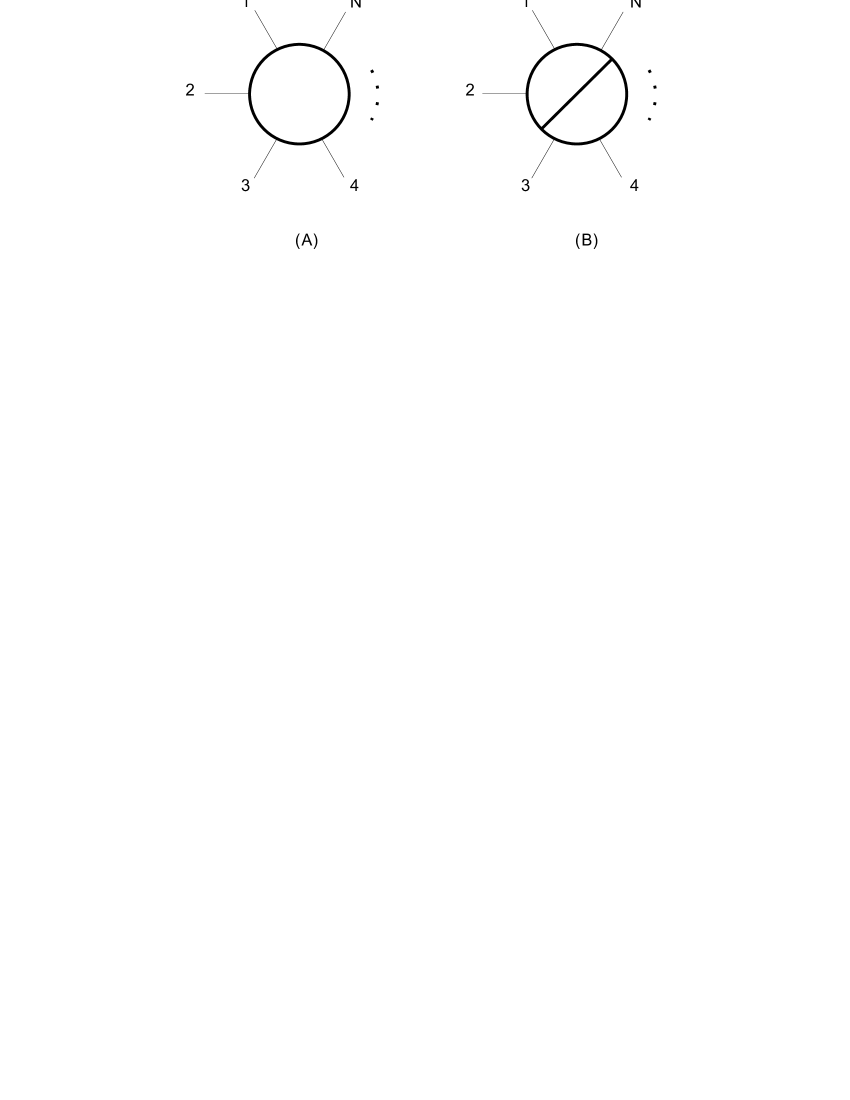
Figure 1: (A) One-loop diagram with $N$ external lines. The topology of a circle has one modulus, the circumference $T$ of the loop. Also there is one residual symmetry, which has to be fixed by taking off one of the proper-time integrals. (B) Two-loop diagrams with $N$ external lines. The topology of this kind has three moduli, the lengths $T_{1}$, $T_{2}$ and $T_{3}$ of the three edges. And there is no unfixed residual symmetry.

The scattering amplitude (4) is a general expression for a worldline of any topology with an arbitrary number of external lines. The form of the vacuum bubble amplitude and Green function depends on the topology. For example, the amplitude of the one-loop 1PI graph with $N$ external lines (Fig. 1(A)) is

$$\mathscr{A}\left({\bigcirc,N}\right)=\int_{0}^{\infty}dT\,\mathscr{V}_{\bigcirc}{\int_{\bigcirc}{\left(\prod\limits_{c=1}^{N-1}{d\tau_{c}}\right)\exp\left[{-\frac{1}{2}\sum\limits_{i,j}{k_{i}\cdot k_{j}G_{\bigcirc}\left({\tau_{i},\tau_{j}}\right)}}\right]}}$$

where

$$\mathscr{V}_{\bigcirc}\left(T\right)=\exp\left(-\frac{1}{2}Tm^{2}\right)T^{-D/2}$$

and

$$G_{\bigcirc}\left({\tau,{\tau}^{\prime}}\right)=-\frac{1}{2}\left[{\left|{\tau-{\tau}^{\prime}}\right|-\frac{\left({\tau-{\tau}^{\prime}}\right)^{2}}{T}}\right]$$

Another example is the amplitude of the two-loop 1PI graph with $N$ external lines (Fig. 1(B)),

$$\mathscr{A}\left({\ominus,N}\right)=\prod\limits_{a=1}^{3}{\int_{0}^{\infty}{dT_{a}}}\,\mathscr{V}_{\ominus}\left(T_{1},T_{2},T_{3}\right){\int_{\ominus}{\left(\prod\limits_{c=1}^{N}{d\tau_{c}}\right)\exp\left[{-\frac{1}{2}\sum\limits_{i,j}{k_{i}\cdot k_{j}G_{\ominus}\left({\tau_{i},\tau_{j}}\right)}}\right]}}$$

where $\mathscr{V}_{\ominus}$ and $G_{\ominus}$ will be determined in the following sections.

III III. Green function

We note that the differential equation (6) is just the Poisson equation the electric potential should satisfy when there is a unit positive charge at ${\tau}^{\prime}$ and a constant negative charge density of magnitude $\rho$ over the whole space. This suggests to us to consider the corresponding static electric problem where the Green function is just the electric potential at $\tau$ of the above setup.

To demonstrate the general solution of the Poisson equation, we solve for the Green function on the two-loop worldline as an example. Consider the 1D topological space as shown in Fig. 2(A) with a unit positive charge at $\tau^{\prime}$ and a unit negative charge uniformly distributed over the whole space. According to the above argument, the Green function $G\left(\tau,\tau^{\prime}\right)$ is the electric potential at $\tau$. Now we can use Gauss’ law and single-valuedness of the potential to write down equations and solve for the expression of the potential. The potential indeed gives a right form for the Green function, but it contains many terms that will be canceled out when calculating the scattering amplitude using equation (4), and hence can be further simplified.

Note that the setup of the static electric problem in Fig. 2(A) can be regarded as the superposition of the 2 setups in Fig. 2(B)(C).

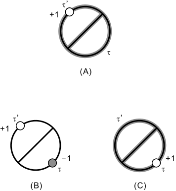
Figure 2: (A) Two-loop topological space with a unit positive charge at $\tau^{\prime}$ and a unit negative charge uniformly distributed over the whole space. (B) Two-loop topological space with a unit positive charge at $\tau^{\prime}$ and a unit negative charge at $\tau$. (C) Two-loop topological space with a unit positive charge at $\tau$ and a unit negative charge uniformly distributed over the whole space.

Let $G\left(\tau,\tau^{\prime}\right)$ denote the potential at $\tau$ of the setup shown in 2(A), and $\bar{G}\left(\tau,\tau^{\prime}\right)$ denote the potential at $\tau$ in Fig. 2(B). The potential at $\tau$ in Fig. 2(C) is then $G\left(\tau,\tau\right)$. Thus

$$G\left(\tau,\tau^{\prime}\right)=\bar{G}\left(\tau,\tau^{\prime}\right)+G\left(\tau,\tau\right)$$

We further define $\tilde{G}\left(\tau,\tau^{\prime}\right)$ as the symmetric part of $\bar{G}\left(\tau,\tau^{\prime}\right)$, i.e.,

$$\tilde{G}\left(\tau,\tau^{\prime}\right)\equiv\frac{1}{2}\left[\bar{G}\left(\tau,\tau^{\prime}\right)+\bar{G}\left(\tau,\tau^{\prime}\right)\right]=\left[\frac{1}{2}G\left(\tau,\tau^{\prime}\right)+\frac{1}{2}G\left(\tau^{\prime},\tau\right)\right]-\frac{1}{2}G\left(\tau,\tau\right)-\frac{1}{2}G\left(\tau^{\prime},\tau^{\prime}\right)$$ (7)

If we use $\tilde{G}\left(\tau,\tau^{\prime}\right)$ instead of $G\left(\tau,\tau^{\prime}\right)$ in equation (4), the sum can be rewritten as

$$-\frac{1}{2}\sum\limits_{i,j}{k_{i}\cdot k_{j}\tilde{G}\left({\tau_{i},\tau_{j}}\right)} = -\frac{1}{2}\sum\limits_{i,j}{k_{i}\cdot k_{j}\left\{\frac{1}{2}\left[G\left({\tau_{i},\tau_{j}}\right)+G\left({\tau_{j},\tau_{i}}\right)-G\left({\tau_{i},\tau_{i}}\right)-G\left({\tau_{j},\tau_{j}}\right)\right]\right\}}$$

$$= -\frac{1}{2}\sum\limits_{i,j}{k_{i}\cdot k_{j}\left\{\frac{1}{2}\left[G\left({\tau_{i},\tau_{j}}\right)+G\left({\tau_{j},\tau_{i}}\right)\right]\right\}}$$

$$= -\frac{1}{2}\sum\limits_{i,j}{k_{i}\cdot k_{j}G\left({\tau_{i},\tau_{j}}\right)}$$

We have used conservation of momentum $\sum{k_{i}}=0$ in the second step and rearranged the summands in the third step. This shows that using $\tilde{G}\left(\tau,\tau^{\prime}\right)$ in equation (4) is equivalent to using $G\left(\tau,\tau^{\prime}\right)$.

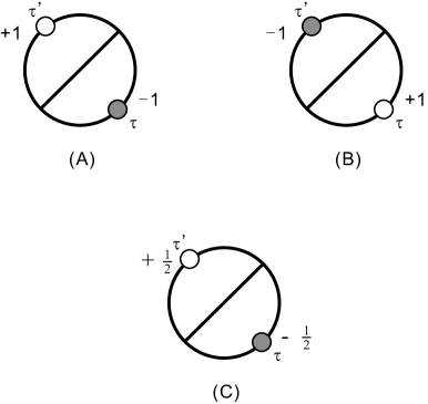
Figure 3: (A) Two-loop topological space with a unit positive charge at $\tau^{\prime}$ and a unit negative charge at $\tau$. (B) Two-loop topological space with a unit negative charge at $\tau^{\prime}$ and a unit positive charge at $\tau$. (C) Two-loop topological space with a half unit positive charge at $\tau^{\prime}$ and a half unit negative charge at $\tau$.

Note that same procedure is usually applied to construct the Green function for bosonic strings D'Hoker:1988ta ,

$$\tilde{G}\left(z,w\right)=G\left(z,w\right)-\frac{1}{2}G\left(z,z\right)-\frac{1}{2}G\left(w,w\right)$$

which is similar to equation (7).

Now we have to look for an electric field analog of $\tilde{G}\left(\tau,\tau^{\prime}\right)$. Since $\bar{G}\left(\tau,\tau^{\prime}\right)$ is the electric potential at $\tau$ of the setup shown in Fig. 3(A), it can be written as the potential at $\tau^{\prime}$ plus the potential difference from $\tau$ to $\tau^{\prime}$. And $\bar{G}\left(\tau^{\prime},\tau\right)$ is the potential at $\tau^{\prime}$ of the setup shown in Fig. 3(B). The sum of $\bar{G}\left(\tau,\tau^{\prime}\right)$ and $\bar{G}\left(\tau^{\prime},\tau\right)$ just gives the potential difference from $\tau$ to $\tau^{\prime}$ of Fig. 3(A) because the potential at $\tau^{\prime}$ of Fig. 3(A) cancels the potential at $\tau^{\prime}$ of Fig. 3(B). $\tilde{G}\left(\tau,\tau^{\prime}\right)$ is half that potential difference, and therefore is just the potential difference from $\tau$ to $\tau^{\prime}$ of Fig. 3(C).

It is now clear that, to write down the expression of the scattering amplitude, we only have to know the symmetric Green function $\tilde{G}$, and use the following formula:

$$\mathscr{A}(\mbox{M},N)=\prod_{a=1}^{\mu}\int_{\mbox{F}_{a}}dT_{a}\,\mathscr{V}_{\mbox{M}}\prod_{c\notin\mbox{C}}\int_{\mbox{M}}d\tau_{c}\exp\left[-\sum_{i<j}k_{i}\cdot k_{j}\tilde{G}(\tau_{i},\tau_{j})\right]$$ (8)

This simplifies the expression of the Green function.

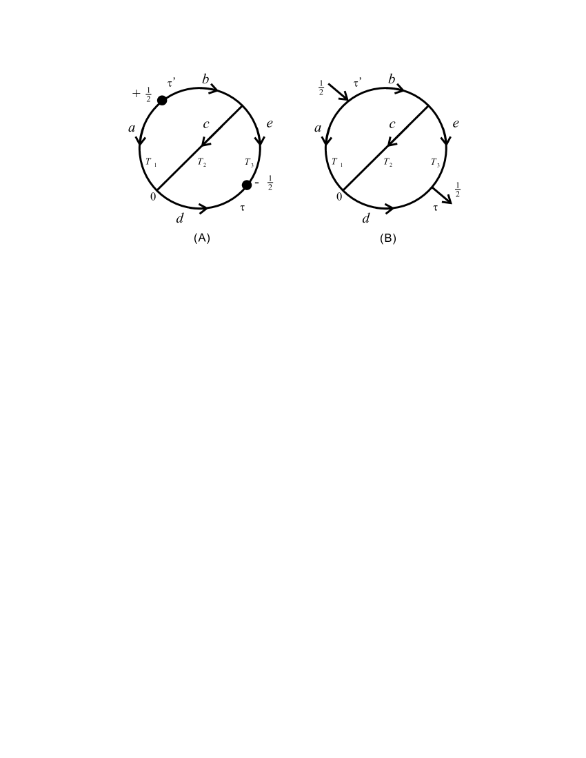
Figure 4: (A) Two-loop topological space with a half unit positive charge at $\tau^{\prime}$ and a half unit negative charge at $\tau$. The lengths of the three arcs are $T_{1}$, $T_{2}$, $T_{3}$. $\tau^{\prime}$ and $\tau$ are respectively on $T_{1}$ and $T_{3}$ and denote the lengths from the origin. The magnitudes of the electric field on each part of the space are denoted by $a$ - $e$ and the directions are chosen arbitrarily. (B) Two-loop circuit with a half unit current input at $\tau^{\prime}$ and withdrawn at $\tau$. The resistances of the three arcs are $T_{1}$, $T_{2}$, $T_{3}$. $\tau^{\prime}$ and $\tau$ are respectively on $T_{1}$ and $T_{3}$ and denote the resistance from the origin. The currents on the parts of the circuit are denoted by $a$ - $e$ and the directions are chosen arbitrarily.

Now that $\tilde{G}(\tau,\tau^{\prime})$ is the potential difference from $\tau$ to $\tau^{\prime}$ in Fig. 3(C), we can apply Gauss’ law (of 1D space) and single-valuedness of the potential to write down the equations the Green function (electric potential $\Phi$) and its first derivative (electric field $E$) should satisfy. We assume the direction and value of $E$ as shown in Fig. 4(A) and $\tau^{\prime}$ and $\tau$ are respectively on $T_{1}$ and $T_{3}$. According to Gauss’ law, we have the following equations:

$$a+b = +\frac{1}{2}$$

$$-a-c+d = 0$$

$$-b+c+e = 0$$

$$-d-e = -\frac{1}{2}$$

The single-valuedness of the potential requires

$$cT_{2}+b(T_{1}-\tau^{\prime}) = a\tau^{\prime}$$

$$cT_{2}+d\tau = e(T_{3}-\tau)$$

If we regard the electric field $E$ as the current $I$, the electric potential $\Phi$ as the voltage $V$, and the length on the 1D space $l$ as the resistance $r$, these equations are just the Kirchhoff equations of a circuit of the same shape as the worldline and with half unit current going into the circuit at $\tau^{\prime}$ and half unit current coming out at $\tau$, as shown in Fig. 4(B). It is easy to see that this equivalence between 1D static electric field and circuit is valid for an arbitrary 1D topological space. We have the following relations for 1D (note that there is no cross-sectional area in the 1D case):

$$\sigma E = I$$

$$\rho l = r$$

$$\Phi = V$$

where $\sigma$ and $\rho$ ($=1/\sigma$) are respectively the 1D conductivity and resistivity, and the relation $El=\Phi$ is equivalent to Ohm’s law $Ir=V$. In addition, Gauss’ law is equivalent to Kirchhoff’s current law, and the single-valuedness of the potential is equivalent to Kirchhoff’s voltage law. Thus the two problems are indeed equivalent. The Green function $\tilde{G}(\tau,\tau^{\prime})$ on a particular 1D topological space M can be understood as the voltage difference from $\tau$ to $\tau^{\prime}$ when a half unit current is input into the “circuit” (1D space) at $\tau^{\prime}$ and withdrawn at $\tau$.

Above we have shown that in the 1D case the problem of solving for the first-quantized particle Green function, the potential difference in a static electric field and the voltage difference in a circuit are analogous. Before we solve the circuit problem for the Green function, it is interesting to give a complete analogy among the quantities in these three kinds of problems (Table 1).

Table 1: Analogy among quantities in three kinds of problems

  Particle Static electric field Electric circuit Green function $\tilde{G}$ potential difference $\Delta\Phi$ voltage difference $\Delta V$ position $x$ electric potential $\Phi$ voltage $V$ momentum $p$ electric field $E$ current $I$ proper time $\tau$ length $l$ resistance $r$ action $S$ energy $U$ power $P$ external force $F$ electric charge $Q$ emf $\mathscr{E}$  

IV IV. Solving the circuit

The next thing we have to do is to find a general expression for the Green function, i.e., a method to obtain the voltage difference described above. A formula has already been given in graph theory (see, e.g., Bollobas:1979bq ). Here we summarize this result and develop it into a formula which is similar to the known form of the Green function on the 2D worldsheet of bosonic string theory D'Hoker:1988ta .

The voltage difference from $\tau$ to $\tau^{\prime}$ can be obtained by the following steps:

(1) Connect $\tau$ and $\tau^{\prime}$ by a wire with zero resistance.

(2) The resulting graph has vertices $V={v_{1},...,v_{n}}$ and edges $E={e_{1},...e_{m-1},e_{m}}$. Denote by $e_{m}$ the edge (wire) we have just added in. Set the directions of all the edges arbitrarily.

(3) Assign voltage, current and resistance on each edge; they can be written in the form of vectors:

$$\mathbf{U} = (U_{1},U_{2},...,U_{m})^{\mbox{T}}$$

$$\mathbf{I} = (I_{1},I_{2},...,I_{m})^{\mbox{T}}$$

$$\mathbf{r} = (r_{1},r_{2},...,r_{m})^{\mbox{T}}$$

Also define the external-force-driven voltage $\mathbf{u}$, which has, in our case, only one non-zero component (the last one). Assume it has magnitude $1$:

$$\mathbf{u}=(u_{1},u_{2},...,u_{m})^{\mbox{T}}=(0,0,...,1)^{\mbox{T}}$$ (9)

(4) Find all the “independent” loops in the graph: There should be $(m-n+1)$. These loops can be identified by the following method: Choose an arbitrary spanning tree (a connected subgraph that contains all the vertices and is a tree) of the graph. There are always $(m-n+1)$ chords (the edges not belonging to the spanning tree). Adding a chord to the spanning tree will generate a one-loop graph. Thus each chord gives a loop in the graph, and all the loops obtained by this way are independent of each other. Therefore there are $(m-n+1)$ loops. Assign an arbitrary direction to each loop.

(5) Define matrices $\mathcal{B}$, $\mathcal{C}$ and $\mathcal{R}$ as follows:

$${\mathcal{B}_{ij}} = \cases{1&if $v_{i}$ is the initial vertex of $e_{j}$\cr-1&if $v_{i}$ is the terminal vertex of $e_{j}$\cr 0&otherwise\cr}$$

$${\mathcal{C}_{ij}} = \cases{1&if $e_{i}$ is in the same direction of the loop $l_{j}$\cr-1&if $e_{i}$ is in the opposite direction of the loop $l_{j}$\cr 0&otherwise\cr}$$

$${\mathcal{R}_{ij}} = \cases{r_{i}&$i=j$\cr 0&$i\neq j$\cr}$$

(6) With the above definitions, we can write down Kirchhoff’s current law, Kirchhoff’s voltage law and Ohm’s law in compact forms as follows:

$$\mathcal{B}\mathbf{I} = \mathbf{0}$$

$$\mathcal{C}^{\mbox{T}}\mathbf{U} = \mathbf{0}$$

$$\mathbf{U} = \mathcal{R}\mathbf{I}+\mathbf{u}$$

The solution to the current on each edge is

$$\mathbf{I}=-\mathcal{C}\left({\mathcal{C}^{\mbox{T}}\mathcal{RC}}\right)^{-1}\mathcal{C}^{\mbox{T}}\mathbf{u}$$

(7) The total resistance between $\tau$ and $\tau^{\prime}$ (excluding the added [last] edge) is then minus the voltage on the last edge divided by the current on that edge, i.e.,

$$R(\tau,\tau^{\prime})=-\frac{U_{m}}{I_{m}}=-\frac{u_{m}}{I_{m}}=-\frac{1}{I_{m}}$$

The Green function is then minus this resistance times the current, one half, since it is the voltage difference from $\tau$ to $\tau^{\prime}$,

$$\tilde{G}(\tau,\tau^{\prime})=-\frac{1}{2}R(\tau,\tau^{\prime})=\frac{1}{2I_{m}}=-\frac{1}{2\mathbf{u}^{\mbox{T}}\mathcal{C}\left({\mathcal{C}^{\mbox{T}}\mathcal{RC}}\right)^{-1}\mathcal{C}^{\mbox{T}}\mathbf{u}}$$ (10)

where the last step comes from extracting the last component of $\mathbf{I}$ by using the vector $\mathbf{u}$ defined in equation (9).

We can further simplify equation (10), by considering the physical meaning of each part of the denominator:

(1) $\mathcal{C}^{\mbox{T}}\mathbf{u}$ and ${\mathbf{u}}^{\mbox{T}}\mathcal{C}$: Since $\mathbf{u}=\left({0,...,0,1}\right)^{\mbox{T}}$, $\mathcal{C}^{\mbox{T}}\mathbf{u}$ is an $\left({m-n+1}\right)$-component column vector whose $i$th component is the direction of the last ($m$th) edge on the $i$th loop ($1$ for “same”, $-1$ for “opposite”, and $0$ for “not on the loop”). If we appropriately choose our independent loops, we can achieve that the $m$th edge is only on the $\left({m-n+1}\right)$th (last) loop and has the same direction as this loop. This is always achievable in steps: (a) Choose the spanning tree in such a way that the $m$th edge doesn’t belong to the spanning tree, i.e., is a chord. (b) Define the loop generated by adding the $m$th edge to the spanning tree to be the $\left({m-n+1}\right)$th loop. (c) Define the direction of the $\left({m-n+1}\right)$th loop to be the same as the $m$th edge. By doing so, we find that $\mathcal{C}^{\mbox{T}}{\rm{\bf u}}$ is just a $\left({m-n+1}\right)$ component column vector with the last component non-vanishing and of value $1$.

$$\mathcal{C}^{\mbox{T}}\mathbf{u}=\left({0,...,0,1}\right)^{\mbox{T}}$$

And $\mathbf{u}^{\mbox{T}}\mathcal{C}$ is the transpose of $\mathcal{C}^{\mbox{T}}\mathbf{u}$. Define for convenience

$$\mathbf{P}\equiv\mathcal{C}^{\mbox{T}}\mathbf{u}$$

Note that $\mathbf{P}^{\mbox{T}}\mathcal{M}{\mathbf{P}}$ gives the $\left[{\left({m-n+1}\right),\left({m-n+1}\right)}\right]$ component of any matrix $\mathcal{M}$ with dimension $\left({m-n+1}\right)\times\left({m-n+1}\right)$.

(2) $\mathcal{C}^{\mbox{T}}\mathcal{RC}$: $\mathcal{C}^{\mbox{T}}\mathcal{RC}$ is an $\left({m-n+1}\right)\times\left({m-n+1}\right)$ matrix. The components can be interpreted as the sum of the “signed” resistances,

$$\left({\mathcal{C}^{\mbox{T}}\mathcal{RC}}\right)_{ij}=\sum\limits_{k\,\in\,\rm{all\,edges}}{f\left({k,i,j}\right)r_{k}}$$

where $r_{k}$ is the resistance on $k$th edge and $f$ is the “sign”:

$$f(n,i,j)=\cases{1&$n$th edge is on both loops $i$ and $j$ with the same orientation\cr-1&$n$th edge is on both loops $i$ and $j$ with opposite orientations\cr 0&$n$th edge is not on both loops $i$ and $j$\cr}$$ (11)

We define for convenience

$$\mathcal{M}\equiv\pmatrix{\Omega&{\mathbf{v}}\cr{\mathbf{v}^{\mbox{T}}}&s\cr}\equiv\mathcal{C}^{\mbox{T}}\mathcal{RC}$$ (12)

where $\Omega$ is an $\left({m-n}\right)\times\left({m-n}\right)$ matrix, $\mathbf{v}$ is an $\left({m-n}\right)$-component vector, and $s$ is a scalar.

Now the formula for the Green function (10) becomes

$$\tilde{G}=-\frac{1}{2\mathbf{P}^{\mbox{T}}\mathcal{M}^{-1}\mathbf{P}}$$

Since ${\mathbf{P}}^{\mbox{T}}\mathcal{M}^{-1}{\mathbf{P}}$ is just the $\left[{\left({m-n+1}\right),\left({m-n+1}\right)}\right]$ component of $\mathcal{M}^{-1}$, we have

$${\mathbf{P}}^{\mbox{T}}\mathcal{M}^{-1}{\mathbf{P}}=\frac{\det\Omega}{\det\mathcal{M}}$$

So, we have

$$\tilde{G}=-\frac{\det\mathcal{M}}{2\det\Omega}$$

Next we evaluate $\det\mathcal{M}$. By the usual matrix algebra (e.g., defining the determinant by a Gaussian integral and doing the “$m-n$” integrals first),

$$\det\mathcal{M}=\det\pmatrix{\Omega&{\mathbf{v}}\cr{\mathbf{v}^{\mbox{T}}}&s\cr}=({\det\Omega})\left[{s-{\mathbf{v}}^{\mbox{T}}\Omega^{-1}\mathbf{v}}\right]$$

So we have the following expression for the Green function:

$$\tilde{G}=-\frac{\det\mathcal{M}}{2\det\Omega}=-\frac{1}{2}s+\frac{1}{2}{\mathbf{v}}^{\mbox{T}}\Omega^{-1}{\mathbf{v}}$$ (13)

V V. Vacuum bubble

To complete this general method of writing down the scattering amplitude, we need to give the expression for the vacuum bubble amplitude with a given topology $\mathscr{V}_{\mbox{M}}\left(T_{a}\right)$ defined in equation (5). This can always be achieved by evaluating the bubble diagram by the second-quantized method, but here we give a derivation by direct calculation in first-quantization. Note that the path integral (5) is the sum over all possible momentum configurations of the product of the expectation values of the free evolution operator between two states at the ends of each edge:

$$\mathscr{V}_{\mbox{M}}\left(T_{a}\right)=\sum\limits_{\{p\}}\left\{\prod\limits_{a=1}^{\mu}{\left\langle p_{a}\left|e^{-T_{a}\left(p^{2}+m^{2}\right)/2}\right|p_{a}\right\rangle}\right\}=\sum\limits_{\{p\}}\left\{\exp\left[\sum\limits_{a=1}^{\mu}{-\frac{1}{2}T_{a}\left(p_{a}^{2}+m^{2}\right)}\right]\right\}$$

where $p_{a}$ is the momentum of the particle traveling on the $a$th edge. The sum over all the configurations of $p_{a}$ can be written as the the integration over all the possible values of $p_{a}$, but they are not independent from each other. Each of the $\mu$ $p_{a}$’s can be written as a linear combination of $L$ $k_{i}$’s where $L$ is the number of loops of the graph and $k_{i}$ is the loop momentum on the $i$th loop. So the amplitude $\mathscr{V}_{\mbox{M}}\left(T_{a}\right)$ can be written as

$$\mathscr{V}_{\mbox{M}}\left(T_{a}\right)=\exp\left[-\frac{1}{2}\left(\sum\limits_{a=1}^{\mu}{T_{a}}\right)m^{2}\right]\int{\left(\prod\limits_{i}^{L}{dk_{i}}\right)\exp\left[-\frac{1}{2}\underline{\sum\limits_{a=1}^{\mu}{T_{a}\left(\sum\limits_{i=1}^{L}{g_{ai}k_{i}}\right)^{2}}}\right]}$$ (14)

where

$$g_{ai}=\cases{1&edge $a$ has the same direction as loop $i$\cr-1&edge $a$ has the opposite direction to loop $i$\cr 0&edge $a$ is not on loop $i$\cr}$$

It is easy to see the following points: (a) If edge $a$ is on loop $i$, there is a $T_{a}k_{i}^{2}$ term in the underlined sum in equation (14), and vice versa. (b) If edge $a$ is on both loop $i$ and loop $j$, there is a term $2T_{a}k_{i}k_{j}$ in the sum, and vice versa. Further, if on edge $a$ both loops have the same (opposite) direction, there is a positive (negative) sign before the term, and vice versa. Thus if we use the factor $f(a,i,j)$ defined in equation (11), we can write the underlined part in equation (14) in a compact form, and further in terms of the period matrix according to the definition (12), or definition (17) below:

$$\sum\limits_{a=1}^{\mu}{T_{a}\left(\sum\limits_{i=1}^{L}{g_{ai}k_{i}}\right)^{2}}=\sum\limits_{a=1}^{\mu}{\sum\limits_{i,j=1}^{L}{f\left(a,i,j\right)T_{a}k_{i}k_{j}}}=\sum\limits_{i,j=1}^{L}{\left[\sum\limits_{a=1}^{\mu}{f\left(a,i,j\right)T_{a}}\right]k_{i}k_{j}}=\sum\limits_{i,j=1}^{L}{\Omega_{ij}k_{i}k_{j}}$$

The amplitude $\mathscr{V}_{\mbox{M}}\left(T_{a}\right)$ can then be calculated easily:

$$\mathscr{V}_{\mbox{M}}\left(T_{a}\right) = \exp\left[-\frac{1}{2}\left(\sum\limits_{a=1}^{\mu}{T_{a}}\right)m^{2}\right]\int{\left(\prod\limits_{i}^{L}{dk_{i}}\right)\exp\left[-\frac{1}{2}\sum\limits_{i,j=1}^{L}{\Omega_{ij}k_{i}k_{j}}\right]}$$ (15)

$$= \exp\left[-\frac{1}{2}\left(\sum\limits_{a=1}^{\mu}{T_{a}}\right)m^{2}\right]\left(\det\Omega\right)^{-D/2}$$

where $D$ is the dimension of the spacetime.

VI VI. Summary

We now summarize our results for general amplitudes. To find the Green function:

(1) Consider the “circuit” (topology M with two more vertices at $\tau$ and $\tau^{\prime}$ respectively) as a graph. Assign a number to each edge. Define arbitrarily the direction of each edge. Assign a number to each loop. Define arbitrarily the direction of each loop.

(2) Find the period matrix $\Omega$ by the following definition:

$$\Omega_{ij}=\sum\limits_{k\,\in\,\rm{all\,edges}}f(k,i,j)r_{k}$$ (16)

where

$$f(n,i,j)=\cases{1&$n$th edge is on both loops $i$ and $j$ with the same orientation\cr-1&$n$th edge is on both loops $i$ and $j$ with opposite orientations\cr 0&$n$th edge is not on both loop $i$ and $j$\cr}$$

Each $r_{k}$ may be $\tau$, $\tau^{\prime}$, a $T_{a}$ of the topological space M without external lines, $T_{a}-\tau$, or $T_{a}-\tau^{\prime}$. It is obvious that $\Omega$ does not depend on $\tau$ and $\tau^{\prime}$, and only depends on the properties of M: To see this, note that the graph of the circuit has just two more vertices (at positions $\tau$ and $\tau^{\prime}$) than the graph of M and each of them may seperate an edge in the graph of M into two “sub-edges”. But these changes on the graph do not affect the period matrix: They neither give new loops nor eliminate loops and the sub-edges will always be on or off a loop simultaneously. Thus the period matrix of the graph of the circuit is just the period matrix of the graph of M. And one only has to calculate it once for one certain topology,

$$\Omega_{ij}=\sum\limits_{a=1}^{\mu}f(a,i,j)T_{a}$$ (17)

(3) Find a path (call it “reference path”) connecting $\tau$ and $\tau^{\prime}$. Choose its direction arbitrarily. Define the scalar $s$ as the total resistance on the reference path.

(4) Find the vector $\mathbf{v}$ defined as follows:

$$\mathbf{v}_{i}=\sum\limits_{k\,\in\,\rm{all\,edges}}f(k,i,0)r_{k}$$

where “0” means the reference path.

(5) The Green function is given by

$$\tilde{G}=-\frac{1}{2}s+\frac{1}{2}{\mathbf{v}}^{\mbox{T}}\Omega^{-1}{\mathbf{v}}$$

The amplitude is then given by

$$\mathscr{A}\left({\mbox{M},N}\right)=\prod\limits_{a=1}^{\mu}{\int_{\mbox{F}_{a}}{dT_{a}}}\,\mathscr{V}_{\mbox{M}}\prod\limits_{c\notin\mbox{C}}{\int_{\mbox{M}}{d\tau_{c}\exp\left[-\sum\limits_{i<j}{k_{i}\cdot k_{j}\tilde{G}\left({\tau_{i},\tau_{j}}\right)}\right]}}$$

with the Green function as above, and the vacuum bubble amplitude is

$$\mathscr{V}_{\mbox{M}}\left(T_{a}\right)=\exp\left[-\frac{1}{2}\left(\sum\limits_{a=1}^{\mu}{T_{a}}\right)m^{2}\right]\left(\det\Omega\right)^{-D/2}$$

Although we have defined and derived all these quantities $s$, $\mathbf{v}$ and $\Omega$ in terms of the concepts in the circuit problem, it is easy to give the worldline geometric interpretation by noting that the resistance is an analog of the proper time, i.e., the length of the worldline (Table 1). $s$ is just the total proper time of the reference path, and the components of $\mathbf{v}$ are the sums of the “signed” proper time on the common edges of the reference path and each loop. Entries of $\Omega$ are sums of the “signed” proper time on the common edges of each pair of loops. (All the signs are given by $f$.) The components of $\mathbf{v}$ and entries of $\Omega$ can also be expressed as integrals of the “Abelian differentials” on the loops of the worldline,

$$v_{i} = \int_{\tau^{\prime}}^{\tau}{\omega_{i}}$$

$$\Omega_{ij} = \ointctrclockwise_{i}\ {\omega_{j}}$$

where $\omega_{i}$ is the line element on loop $i$ and the second integral is around loop $i$ along its direction. Then our expression for the particle amplitude has a similar structure to the bosonic string amplitude, with the Green function on the 2D worldsheet D'Hoker:1988ta :

$$\tilde{G}\left(w,z\right)=-2\ln\left|E\left(w,z\right)\right|+2\pi\ \text{Im}\int_{w}^{z}\mathbf{\omega}\left(\text{Im}\ \Omega\right)^{-1}\text{Im}\int_{w}^{z}\mathbf{\omega}$$

where $E$ is the prime form, the vector $\mathbf{\omega}$ contains the basis of the Abelian differentials and the matrix $\Omega$ is the period matrix.

VII VII. Examples

Here we give some examples of obtaining the Green functions on different topologies. For the finite line of length $T$ in Fig. 5, there is no loop, so there is no period matrix $\Omega$ nor vector $\mathbf{v}$. $s$ is just the total resistance between $\tau$ and $\tau^{\prime}$. So the Green function is

$$\tilde{G}_{-}\left(\tau,\tau^{\prime}\right)=-\frac{1}{2}s=-\frac{1}{2}\left|{\tau-\tau^{\prime}}\right|$$

and

$$\mathscr{V}_{-}\left(T\right)=\exp\left(-\frac{1}{2}Tm^{2}\right)$$

The amplitude is then given by equation (8). One just has to note that there is one modulus $T$ for this case and to fix the residual symmetry: Two of the external lines should be fixed at one end of the line and another two should be fixed at the other end.

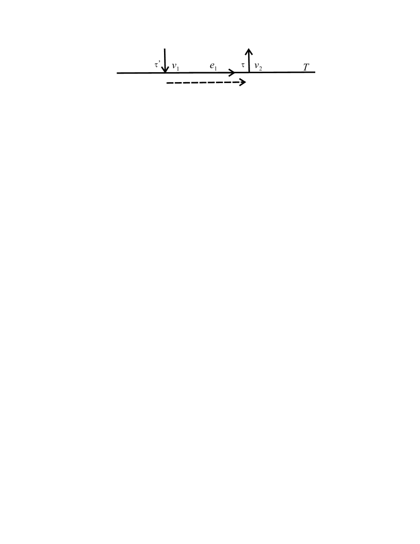
Figure 5: The topology of a line with length $T$. There is no loop and hence no period matrix nor vector $\mathbf{v}$. The only path between $\tau$ and $\tau^{\prime}$ is the edge connecting the two vertices $e_{1}$, so we choose it as the reference path.

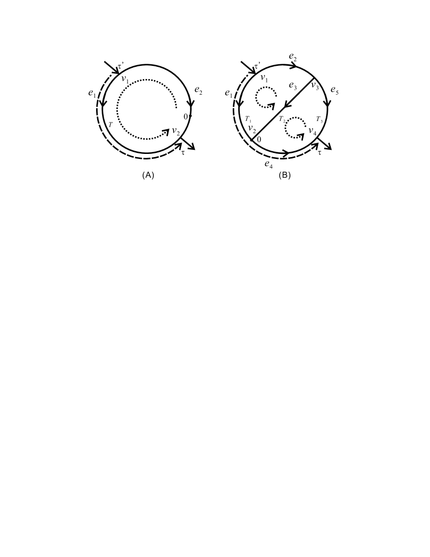
Figure 6: (A) The one-loop topology. $T$ is the circumference of the circle. There are two edges ($e_{1}$,$e_{2}$) and two vertices ($v_{1}$,$v_{2}$). $\tau$ and $\tau^{\prime}$ are the lengths from $v_{1}$ and $v_{2}$ to the origin though a counterclockwise path. The directions of the edges are chosen arbitrarily and marked in the figure. There is only one loop and it is marked by dotted lines. The reference path is marked by a dashed line. (B) A two-loop topology. $T_{1}$, $T_{2}$ and $T_{3}$ are the lengths of the three arcs. $\tau$ and $\tau^{\prime}$ are respectively the length on the 3rd and 1st arc from the origin. (If the Green function with $\tau$ and $\tau^{\prime}$ on different arcs is needed, simply repeat the steps for this special case.) There are 5 edges ($e_{1}$ to $e_{5}$) and 4 vertices ($v_{1}$ to $v_{4}$). The directions of the edges are chosen arbitrarily and marked in the figure. There are two independent loops and they are marked by dotted lines. The reference path is marked by a dashed line.

For the circle, there is one loop as shown in Fig. 6(A). So the period matrix is $1\times 1$. The only entry of $\Omega$ is then

$$\Omega=T$$

And according to the definition, $s$ and $\mathbf{v}$ are

$$s=\left|{\tau-\tau^{\prime}}\right|$$

$$\mathbf{v}=\left|{\tau-\tau^{\prime}}\right|$$

Thus the Green function on the circle is

$$\tilde{G}_{\bigcirc}\left(\tau,\tau^{\prime}\right)=-\frac{1}{2}s+\frac{1}{2}{\mathbf{v}}^{\mbox{T}}\Omega^{-1}{\mathbf{v}}=-\frac{1}{2}\left|{\tau-\tau^{\prime}}\right|+\frac{(\tau-\tau^{\prime})^{2}}{2T}$$

and the vacuum bubble amplitude is

$$\mathscr{V}_{\bigcirc}\left(T\right)=\exp\left(-\frac{1}{2}Tm^{2}\right)T^{-D/2}$$

For the Green function on the 2-loop graph shown in Fig. 6(B), the period matrix is $2\times 2$ and $\mathbf{v}$ is a two-component vector. $\Omega$, $s$ and $\mathbf{v}$ are

$$\Omega = \pmatrix{T_{1}+T_{2}&-T_{2}\cr-T_{2}&T_{2}+T_{3}\cr}$$

$$s = \tau^{\prime}+\tau$$

$$\mathbf{v} = (\tau^{\prime},\tau)^{\mbox{T}}$$

So the Green function is, by plugging all the above into equation (13),

$$\tilde{G}_{\ominus}\left(\tau,\tau^{\prime}\right)=-\frac{T_{1}\left({T_{2}+T_{3}-\tau}\right)\tau+T_{1}\left({T_{2}+T_{3}}\right){\tau}^{\prime}-T_{3}{\tau}^{\prime 2}+T_{2}\left({T_{3}-\tau-{\tau}^{\prime}}\right)\left({\tau+{\tau}^{\prime}}\right)}{2\left({T_{1}T_{2}+T_{2}T_{3}+T_{3}T_{1}}\right)}$$

and the vacuum bubble amplitude is

$$\mathscr{V}_{\ominus}\left(T_{1},T_{2},T_{3}\right)=\exp\left[-\frac{1}{2}\left(T_{1}+T_{2}+T_{3}\right)m^{2}\right]\left(T_{1}T_{2}+T_{2}T_{3}+T_{3}T_{1}\right)^{-D/2}$$

VIII VIII. Conclusions

Based on the first-quantized formalism, the discussion in this paper gives a new method to evaluate the scattering amplitude of scalar field theory at arbitrary loop level. (The procedure was given in section VI.) The form of the Green function is shown to be similar to that on the worldsheet in bosonic string theory. The method applies not only to 1PI graphs, but arbitrary graphs that might appear in S-matrices.

The amplitude obtained by the first-quantized method in this paper easily can be shown to be equivalent to the amplitude from second-quantization. Further, the singularities of general diagrams can be discussed and the Landau conditions can be obtained. The occurrence of a singularity on the physical boundary was shown to be related to a sequence of interactions connected by real particle paths by Coleman and Norton Coleman:1965xm . Here this same picture emerges more naturally: The Feynman diagram is interpreted as particle path (through background fields) and the integral over the proper time is introduced from the beginning.

The extension to diagrams with spinning particles will be the next thing to understand. It is expected to be parallel to Strassler’s discussion on various theories Strassler:1992zr , with the Green function on a circle replaced by those on other topologies. However, although the 2-loop Green function has been known for a long time, no full-fledged extension to even 2-loop Yang-Mills theory has yet been found, because of the complexity and difficulty entering at multi-loop level. Previous attempts include generalization from Bern and Kosower’s string approach DiVecchia:1995in DiVecchia:1996uq and Strassler’s particle approach Sato:1998sf Sato:2000cr .

It is now clear that scalar field theory can be seen as the limit of the bosonic string theory, by suppressing the length of the string. Can the bosonic string worldsheet be seen as the sum of all the Feynman diagrams of the scalar field theory that are random lattices of the worldsheet? This is another interesting question that may be related to the result in this paper.

References

- (1) R. P. Feynman, Phys. Rev. 80, 440 (1950).
- (2) Y. Nambu, Prog. Theor. Phys. 5, 82 (1950).
- (3) J. S. Schwinger, Phys. Rev. 82, 664 (1951).
- (4) Y. Nambu, Proc. of International conference on Symmetries and quark model, Detroit, USA, June 1969. L. Susskind, Phys. Rev. D 1, 1182 (1970), Nuo. Cim. 69A, 457 (1970). H.B. Nielsen, 15th international conference on high energy physics, Kiev, Ukraine, Sept. 1970.
- (5) Z. Bern and D. A. Kosower, Nucl. Phys. B 379, 451 (1992).
- (6) Z. Bern and D. C. Dunbar, Nucl. Phys. B 379, 562 (1992).
- (7) M. J. Strassler, Nucl. Phys. B 385, 145 (1992) [arXiv:hep-ph/9205205].
- (8) M. G. Schmidt and C. Schubert, Phys. Lett. B 331, 69 (1994) [arXiv:hep-th/9403158].
- (9) K. Roland and H. T. Sato, Nucl. Phys. B 480, 99 (1996) [arXiv:hep-th/9604152].
- (10) J. Mathews, Phys. Rev. 113, 381 (1959).
- (11) J. D. Bjorken, PhD thesis, Stanford University, 1959. J. D. Bjorken and S. D. Drell, Relativistic Quantum Field Theory, McGraw-Hill, 1965, p. 220-226
- (12) D. B. Fairlie and H. B. Nielsen, Nucl. Phys. B 20, 637 (1970).
- (13) E. P. Verlinde and H. L. Verlinde, Nucl. Phys. B 288, 357 (1987). E. D’Hoker and D. H. Phong, Rev. Mod. Phys. 60, 917 (1988).
- (14) B. Bollobas, Graph Theory, Springer-Verlag, 1979, p. 40.
- (15) S. Coleman and R. E. Norton, Nuovo Cim. 38, 438 (1965).
- (16) P. Di Vecchia, A. Lerda, L. Magnea and R. Marotta, Phys. Lett. B 351, 445 (1995) [arXiv:hep-th/9502156].
- (17) P. Di Vecchia, L. Magnea, A. Lerda, R. Russo and R. Marotta, Nucl. Phys. B 469, 235 (1996) [arXiv:hep-th/9601143].
- (18) H. T. Sato and M. G. Schmidt, Nucl. Phys. B 560, 551 (1999) [arXiv:hep-th/9812229].
- (19) H. T. Sato, M. G. Schmidt and C. Zahlten, Nucl. Phys. B 579, 492 (2000) [arXiv:hep-th/0003070].