Dynamical Generation of Non-Abelian Gauge Group
via the Improved Perturbation Theory

Abstract

It was suggested that the massive Yang-Mills-Chern-Simons matrix model has three phases and that in one of them a non-Abelian gauge symmetry is dynamically generated. The analysis was at the one-loop level around a classical solution of fuzzy sphere type. We obtain evidences that three phases are indeed realized as nonperturbative vacua by using the improved perturbation theory. It also gives a good example that even if we start from a trivial vacuum, the improved perturbation theory around it enables us to observe nontrivial vacua.

I Introduction

It is now widely believed that some gauge theories or matrix models would provide nonperturbative formulations of string theories in the large-$N$ limit Banks:1996vh ; Ishibashi:1996xs ; Maldacena:1997re . In such approaches, it is quite important to clarify how they quantize gravity, namely, how they reconcile the general relativity and quantum theory. It is also of great importance to confirm whether at a low energy regime they can be effectively described by quantum field theories of gauge fields with the non-Abelian gauge group of the standard model type. However, in the context of the matrix models it is not yet known how the gauge group of the standard model is dynamically generated. It is natural that it is embedded in the original ${\it U}(N)$ gauge group of a matrix model we start from and that it emerges dynamically in the large-$N$ limit Iso:1999xs via the Higgs mechanism or the confinement, for example. Therefore, it is interesting and necessary to construct matrix models that incorporate such a mechanism and to study them in a nonperturbative manner.

As a first step toward this program, the bosonic massive Yang-Mills-Chern-Simons (YMCS) matrix model was analyzed in Ref. Azuma:2005bj , which is obtained by the large-$N$ reduction Kawai:1982nm of the ${\it U}(N)$ Yang-Mills theory with the Chern-Simons term in three dimensions and by adding the mass term. Without the mass term, it was shown in Ref. Azuma:2004zq that the YMCS matrix model has two phases, namely, the Yang-Mills phase and the fuzzy sphere phase. In the former phase observables show qualitatively the same behavior as those in the pure Yang-Mills model without the Chern-Simons term, while in the latter a single fuzzy sphere is a stable and dominant configuration due to the Chern-Simons term. It was claimed in Ref. Azuma:2005bj that if the mass term is present there appears an interesting third phase (“5-brane phase”) in addition to these two phases, in which a dominant configuration is expected to be $\mathcal{O}(N)$ coincident fuzzy spheres of small size and thus a non-Abelian gauge group with rank of $\mathcal{O}(N)$ is dynamically generated as a subgroup of the original ${\it U}(N)$ gauge group Iso:2001mg . Although in the fuzzy sphere phase comparison between the one-loop calculation around a single fuzzy sphere configuration and the Monte Carlo data shows one-loop dominance, namely higher-loop corrections are suppressed in the large-$N$ limit as long as 1PI diagrams are concerned Azuma:2004zq , it is not a priori trivial whether the analysis at the one-loop level is sufficient even in the presence of mass term.

In order to examine whether the 5-brane phase found in Ref. Azuma:2005bj is indeed realized as a nonperturbative vacuum, we have to investigate the massive YMCS matrix model in a nonperturbative method. Toward this aim, we employ here the improved perturbation theory developed in Ref. Kawai:2002jk , which is motivated by the improved mean field approximation (IMFA). This concept is also called the Gaussian approximation or Gaussian expansion method and was introduced to a large-$N$ reduced model in Ref. Kabat:1999hp ; Oda:2000im , which has been further investigated in various manners Nishimura:2001sx ; Kawai:2002ub ; Nishimura:2002va . This technique is a sort of variational method Stevenson:1981vj to extract nonperturbative information on the vacuum of a theory. The IMFA is indeed reduced to the standard mean field approximation at the leading order, and the inclusion of higher-order contributions may be viewed as systematic improvement of the approximation. The IMFA has been applied successfully to a number of models to yield nonperturbative results Kawai:2002jk ; Kabat:1999hp ; Oda:2000im ; Nishimura:2001sx ; Kawai:2002ub ; Nishimura:2002va ; Zhong:2003xr ; Kawamoto:2003kn ; Aoyama:2006di ; Aoyama:2006je ; Aoyama:2005nd . In particular, the IMFA was applied to the IIB matrix model first in Ref. Nishimura:2001sx and provided the interesting nonperturbative observation that our four-dimensional space-time is realized in the IIB matrix model as the anisotropy of eigenvalue distribution of ten bosonic Hermitian matrices. This result was further confirmed in Refs. Kawai:2002jk ; Kawai:2002ub ; Aoyama:2006di ; Aoyama:2006je .

The improved perturbation theory was developed as such a reformulation of the IMFA that it is considered as a reorganization of a perturbative series. It opened a way to taking account of more general types of action than that had been treated in the IMFA or the Gaussian expansion method. Thus in the present article we examine the matrix model with Chern-Simons term that has a cubic interaction term in the framework of the improved perturbation theory. We expect that the observations obtained in this work would be instructive to future studies of more nontrivial and interesting nonperturbative phenomena via the improved perturbation theory, in particular, dynamical generation of gauge symmetry in the IIB matrix model.

In the prescription of the IMFA and the improved perturbation theory, a set of artificial parameters are introduced through a nominal deformation in the original action of the model. It leads to a sort of consistency conditions for these parameters that the original theory should not depend on them. In the space of these parameters, the conditions may be realized as a region in which physical quantities are least sensitive to the variation of the parameters Stevenson:1981vj . Such a region is called “plateau”. As stressed in Refs. Kawai:2002jk ; Kawai:2002ub , formation of a plateau provides an essential criterion to see whether or not the improved perturbation theory works. It is shown in Ref. Aoyama:2005nd that in a system which exhibits a phase transition, there may appear several plateaux. Therefore, it is interesting to discuss the phase structure of the massive YMCS matrix model in the framework of the improved perturbation theory through the patterns of emergence of plateaux that correspond to various phases.

Another motivation of applying the improved perturbation theory to the massive YMCS matrix model comes from the fact that even if we start from the perturbative vacuum, the improved perturbation theory can provide information on a nonperturbative vacuum which does not always correspond to a classical configuration. Therefore, in principle, even if we start from the trivial vacuum which corresponds to the Yang-Mills phase, we would be able to identify the fuzzy sphere phase and the 5-brane phase when they are realized as nonperturbative vacua. We will see that this is indeed the case. This is in contrast with previous analyses of fuzzy sphere type configurations based on the perturbation theory around them Azuma:2005bj ; Azuma:2004zq ; Imai:2003vr ; Azuma:2004yg .

The organization of this paper is as follows: in the next section we review the massive YMCS matrix model and its three phases. In Section III, we also give a review of the improved perturbation theory, which is applied to the massive YMCS matrix model in Section IV. The results are presented in Section V. Section VI is devoted to discussions. The tables are put collectively at the end of the paper.

II The model

The massive Yang-Mills-Chern-Simons matrix model is defined by the action

$$S=N{\rm tr}\left(-\frac{1}{4}[A_{\mu},A_{\nu}]^{2}+\frac{i}{3}\alpha\epsilon_{\mu\nu\lambda}A_{\mu}A_{\nu}A_{\lambda}+\frac{1}{2}m^{2}A_{\mu}^{2}\right),$$ (1)

where $A_{\mu}$ ($\mu=1\sim 3$) are $N\times N$ Hermitian matrices. We will consider this model in the large-$N$ limit. We can obtain this model by adding the mass term to the large-$N$ reduced model of the ${\it U}(N)$ Yang-Mills theory with the Chern-Simon term in three dimensions. This model has two parameters $\alpha$, $m$ and we are interested in the free energy of this model

$$F=-\frac{1}{N^{2}}\log Z,\qquad Z=\int dA_{\mu}\,e^{-S},$$ (2)

as a function of them, by which we can determine the phase structure of this model.

The equation of motion derived from Eq. (1) is

$$[A_{\lambda},[A_{\lambda},A_{\mu}]]+\frac{i}{2}\alpha\epsilon_{\mu\nu\lambda}[A_{\nu},A_{\lambda}]+m^{2}A_{\mu}=0.$$ (3)

Apart from a trivial solution $A_{\mu}=0$, this model admits a classical solution of fuzzy sphere type given by

$$A_{\mu}=\chi L_{\mu},\qquad\mu=1\sim 3,$$ (4)

where $L_{\mu}$’s is the $N$-dimensional representation of ${\it SU}(2)$ algebra satisfying

$$[L_{\mu},L_{\nu}]=i\epsilon_{\mu\nu\lambda}L_{\lambda},$$ (5)

and $\chi=(\alpha+\sqrt{\alpha^{2}-8m^{2}})/4$. If $m^{2}>\alpha^{2}/8$, this type of solution ceases to exist. Generically $L_{\mu}$ can be a reducible representation of the ${\it SU}(2)$ algebra which consists of the $n_{i}$-dimensional irreducible representations for $i=1\sim s$, where $\sum_{i=1}^{s}n_{i}=N$. In this case without loss of generality $A_{\mu}$ can be brought into the form

$$A_{\mu}=\chi\begin{pmatrix}L_{\mu}^{(n_{1})}&&&\\ &L_{\mu}^{(n_{2})}&&\\ &&\ddots&\\ &&&L_{\mu}^{(n_{s})}\\ \end{pmatrix},$$ (6)

where $L_{\mu}^{(n)}$ denotes the $n$-dimensional irreducible representation. Substituting this into the action (1), we obtain the classical action of this solution as

$$S_{\text{cl}}=Nf(\chi)\sum_{i=1}^{s}\frac{n_{i}(n_{i}^{2}-1)}{4},$$ (7)

where $f(\chi)=\chi^{4}/2-\alpha\chi^{3}/3+m^{2}\chi^{2}/2$. When $\alpha^{2}>9m^{2}$, $f(\chi)$ is always negative, thus Eq. (7) implies that a single fuzzy sphere ($s=1$, $n_{1}=N$) is the most dominant configuration as long as $\alpha^{2}$ and $m^{2}$ are not so small that $S_{\text{cl}}\sim\mathcal{O}(1)$. Then the system is in the fuzzy sphere phase. On the other hand, when $\alpha^{2}<9m^{2}$, $f(\chi)>0$ and the trivial solution $A_{\mu}=0$ becomes stable. Moreover, whenever $\alpha$ is so small, the one-loop analysis around a background

$$A_{\mu}=\text{diag}(x_{\mu}^{(1)},x_{\mu}^{(2)},\cdots,x_{\mu}^{(N)}),$$ (8)

shows that in general there is an attractive force between the eigenvalues of $A_{\mu}$, and it makes their distribution shrink until the perturbative calculation becomes no longer valid Hotta:1998en . Then they form a “solid ball” and the system is in the Yang-Mills phase. However, as shown in Ref. Azuma:2005bj , this is not the end of the story. So far we have discussed the phase of the model based on the classical action (7). If we take account of the one-loop contribution to the free energy, we can find the third phase for the moderate $\alpha$ and $m$ satisfying $8m^{2}<\alpha^{2}<9m^{2}$ in which $\mathcal{O}(N)$ copies of the small fuzzy sphere appear as the true vacuum. This phase is called “5-brane phase” in Ref. Azuma:2005bj because this configuration is analogous to the one that is interpreted Maldacena:2002rb as coinciding transverse 5-branes in the BMN matrix model Berenstein:2002jq . By considering configurations with fuzzy spheres of various sizes, the phase diagram was proposed in Ref. Azuma:2005bj at the one-loop level. The one-loop calculation is reliable in some parameter regions provided that the perturbative series around classical configurations are well-defined.

However, in a general parameter region it is not clear that the one-loop calculation is sufficient and even if so, the perturbative series would be asymptotic. Therefore, it is interesting to confirm that the phase diagram in Ref. Azuma:2005bj is true even at a nonperturbative level by a totally different method. As such, we employ the improved perturbation theory developed in Ref. Kawai:2002jk , which works well even for some asymptotic series.

III The improved perturbation theory

In order to describe the idea of the improved perturbation theory, we consider as an illustration a one-matrix model defined by the action

$$S=\frac{N}{4}{\rm tr}\phi^{4},$$ (9)

where $\phi$ is an $N\times N$ Hermitian matrix. Suppose we are interested in the free energy

$$N^{2}F=-\log\int d\phi\exp\left(-\frac{N}{4}{\rm tr}\phi^{4}\right),$$ (10)

which cannot be computed by the standard perturbation theory for lack of the mass term (quadratic term) in Eq. (9). Therefore, let us formally add and subtract the mass term in the action, one of which is regarded as a perturbation. Then we introduce a formal coupling constant $g$ and construct a perturbative series in terms of $g$. $g$ will be taken to be 1 in the end:

$$N^{2}F=\left.-\log\int d\phi\exp\left(-N{\rm tr}\left(\frac{g}{4}\phi^{4}-g\frac{m_{0}^{2}}{2}\phi^{2}+\frac{m_{0}^{2}}{2}\phi^{2}\right)\right)\right|_{g=1},$$ (11)

where $m_{0}$ is an artificially introduced parameter. It can be restated in the following way. If we define the free energy of a massive theory as

$$N^{2}F(m^{2})=-\log\int d\phi\exp\left(-N{\rm tr}\left(\frac{g}{4}\phi^{4}+\frac{m^{2}}{2}\phi^{2}\right)\right),$$ (12)

the prescription above is equivalent to calculating the free energy of the massless theory (10) from the massive theory with mass parameter replaced as

$$F(0)\bigl{|}_{g=1}=F(m_{0}^{2}-gm_{0}^{2})\bigr{|}_{g=1}.$$ (13)

The perturbative series in terms of $g$ obtained from the RHS of Eq. (13) is called the improved perturbative series. Note that if we can sum up this series at the full order, the free energy is completely independent of $m_{0}$ which is introduced artificially in order to make the perturbation theory feasible.

In practice, we can calculate the RHS in Eq. (13) only up to a finite order. Then the dependence on $m_{0}$ emerges in the improved perturbative series. In order to obtain the exact value of the free energy, we need to determine the value of $m_{0}$ somehow. Here we adopt the principle of minimal sensitivity Stevenson:1981vj as a guiding principle: the improved series should depend least on $m_{0}$. It is because the original theory does not depend on $m_{0}$ which was introduced through a nominal shift of parameter. If there exists a region in the parameter space of $m_{0}$ where the dependence on $m_{0}$ vanishes effectively, the exact value would be reproduced there. We call such a region as “plateau”. The principle of minimal sensitivity is realized as the emergence of plateau, in which the improved series stays stable against any variation of the artificial parameter.

As for the one-matrix model (10), we can identify a clear plateau even up to the 8th order, and there the improved perturbative series reproduces the exact value of the free energy with more than 99.5% accuracy Kawai:2002ub . It is a striking result that although the original perturbative series of the massive theory has a radius of convergence $g/m^{4}<1/12$ Brezin:1977sv , we have obtained a good approximate value at $m=0$ by this technique. The plausibility and applicability of the improved perturbation theory is not yet clear in the mathematically strict sense. Nevertheless it has been successfully used in various models. Some examples are also given in Ref. Kawai:2002jk .

Note that at the first order in $g$ if we require $\partial F_{1}^{\text{imp}}/\partial m_{0}=0$ as a “plateau” condition, this reduces to the self-consistency condition in the standard mean field approximation. In this sense, the improved perturbation series is a natural generalization of the mean field approximation.

The scheme presented so far can be generalized to a generic series that may have more than one parameter. Thus we arrive at the concept of the improved Taylor expansion Kawai:2002jk as follows. Let us assume that an observable of a theory would be exactly described by a function $F(\lambda,\xi)$. Here $\lambda$ is a coupling constant and $\xi$ collectively represents parameters of the model such as a mass. Perturbation theory provides an expansion of $F$ as a power series of $\lambda$ about $\lambda=0$, with $n$th coefficient denoted as $f_{n}(\xi)$:

$$F(\lambda,\xi)=\sum_{n=0}^{\infty}\,\lambda^{n}\,f_{n}(\xi)\,.$$ (14)

Next we consider a modification of the series according to the following prescriptions. First we perform a shift of parameters:

$$\lambda \longrightarrow g\,\lambda\,,$$

$$\xi \longrightarrow\xi_{0}+g(\xi-\xi_{0}),$$ (15)

where we have introduced $g$ as a formal expansion parameter, and $\xi_{0}$ as a set of artificial parameters. We deform the series by the substitution (15), and then we reorganize the series in terms of $g$ up to $g^{k}$ and drop the $\mathcal{O}(g^{k+1})$ terms, and finally set $g$ to 1. Thus we obtain the improved perturbative series $F^{\text{imp}}_{k}$ as

$$F(\lambda,\xi)\,\longrightarrow\,F^{\text{imp}}_{k}(\lambda,\xi;\xi_{0})=\left.F(g\lambda,\xi_{0}+g(\xi-\xi_{0}))\right|_{\text{up to}~{}\mathcal{O}(g^{k}),~{}g=1}.$$ (16)

Here, a notation $\bigr{|}_{\text{up to}~{}\mathcal{O}(g^{k}),~{}g=1}$ represents the operation that we disregard the $\mathcal{O}(g^{k+1})$ terms and then put $g$ to 1.

More concretely, the improved perturbative series up to $k$th order $F^{\text{imp}}_{k}$ is made by the procedure:

$$F_{k}(\xi) \equiv \sum_{n=0}^{k}\,\lambda^{n}\,f_{n}(\xi)$$ (17)

$$\longrightarrow \sum_{n=0}^{k}\,(g\lambda)^{n}\,f_{n}(\xi_{0}+g(\xi-\xi_{0}))$$ (18)

$$= \sum_{\ell=0}^{\infty}\,g^{\ell}\,\sum_{n=0}^{\min(k,\ell)}\,\lambda^{n}\,\frac{1}{(\ell-n)!}\,(\xi-\xi_{0})^{\ell-n}\,f_{n}^{(\ell-n)}(\xi_{0})$$ (19)

$$\longrightarrow \sum_{\ell=0}^{k}\,g^{\ell}\,\sum_{n=0}^{\ell}\,\lambda^{n}\,\frac{1}{(\ell-n)!}\,(\xi-\xi_{0})^{\ell-n}\,f_{n}^{(\ell-n)}(\xi_{0})$$ (20)

$$\longrightarrow \sum_{n=0}^{k}\,\lambda^{n}\,\sum_{\ell=0}^{k-n}\,\frac{1}{\ell!}\,(\xi-\xi_{0})^{\ell}\,f_{n}^{(\ell)}(\xi_{0})$$ (21)

$$\equiv F^{\text{imp}}_{k}(\lambda,\xi;\xi_{0})\,.$$ (22)

Here, $f_{n}^{(\ell)}$ is the $\ell$th derivative of $f_{n}(\xi)$ with respect to $\xi$. At first we apply the transformation (15) to the original $k$th order perturbative series in Eq. (18). Next the series is then reorganized in terms of $g$ in Eq. (19). At this stage, we must take into account the extra $g$-dependence as $\xi_{0}+g(\xi-\xi_{0})$ in the coefficient $f_{n}$. Then we drop the $\mathcal{O}(g^{k+1})$ terms in Eq. (20), and finally set $g$ to 1 in Eq. (21). In this way we obtain the improved series $F^{\text{imp}}_{k}$ (22).

It turns out that by the procedure of the improved perturbation theory, each coefficient of the original series $f_{n}(\xi)$ are replaced by a particular combination of the coefficients in its Taylor expansion about a shifted point $\xi_{0}$,

$$f_{n}(\xi)\longrightarrow\widetilde{f_{n}}(\xi;\xi_{0})=\sum_{\ell=0}^{k-n}\,\frac{1}{\ell!}\,(\xi-\xi_{0})^{\ell}\,f_{n}^{(\ell)}(\xi_{0}).$$ (23)

From this expression, we immediately find that even if $F_{k}(\xi)$ in Eq. (17) shows worse behavior, the improved perturbative series $F_{k}^{\text{imp}}(\xi;\xi_{0})$ in Eq. (22) often becomes mild as a function of $\xi$.

In this procedure, the foregoing example of one matrix model corresponds to a case of $\lambda=1$ and $\xi\equiv m^{2}=0$ where the improved perturbative series $F^{\text{imp}}_{k}$ boils down to the expression (13).

Because the emergence of a plateau is an essential criterion to see whether the improved perturbation theory works well, a main task is identification of plateau with respect to the artificial parameter $\xi_{0}$ at each value of the parameter $\xi$. Although we do not yet have a rigorous definition of plateaux, we could identify them by their properties investigated in Kawai:2002jk ; Kawai:2002ub ; Aoyama:2005nd ; Aoyama:2006je as follows. The ideal realization of the plateau may have such a property that the improved series is totally independent of the artificial parameters $\xi_{0}$ in a certain region. It involves a situation that all orders of derivatives of the improved series with respect to $\xi_{0}$ are zero in that region. However, such an ideal plateau is not realized in practical cases because we have series only of finite order. Typical profile of the improved series that forms plateau exhibits a flat region in which the series fluctuates bit by bit; it would consist of a number of local maxima and minima. Thus, we consider the accumulations of extrema as indications of plateau (or its candidates).

In some cases it occurs that there is a region in which $F^{\text{imp}}_{k}$ becomes stable but varies gently without forming extrema. We should also take into account this region as a plateau. However, we have to mention that we often exclude such an asymptotic behavior that the series becomes flat at large values of parameters $\xi_{0}$.

For each value of $\xi$, there may appear more than one plateau, each of which corresponds to either a stable physical state or an unstable or metastable state (local minimum). By comparing the values of the improved free energy at these plateaux in the parameter space of $\xi_{0}$, we are able to discuss which one is realized as a vacuum at the specified values of parameters $\xi$. The phase transition may also be argued on this basis in such a way that the state corresponding to the vacuum changes under the variation of the parameters $\xi$.

It should be noted that although the free energy is a generating function of all observables which are obtained as derivatives with respect to corresponding parameters $\xi$, analyses of the improved perturbation theory should be applied independently to each observable of interest. This is because the prescription of improvement does not commute with differentiation with respect to the parameters $\xi$ and thus the formation of plateau may occur in a different manner by observables especially at lower orders of perturbation.

IV Application to the massive Yang-Mills Chern-Simons matrix model

In this section we discuss how to apply the improved perturbation theory to the massive YMCS matrix model. In order to determine the phase structure, we concentrate on the free energy $F(\alpha,m^{2})$ given in Eq. (2) and the expectation value of the Chern-Simons term

$$A(\alpha,m^{2})\equiv\frac{\partial F(\alpha,m^{2})}{\partial\alpha}=\left\langle\frac{1}{N}{\rm tr}\left(\frac{1}{3}i\epsilon_{\mu\nu\lambda}A_{\mu}A_{\nu}A_{\lambda}\right)\right\rangle,$$ (24)

as functions of two parameters $\alpha$, $m$ appearing in Eq. (1). The reason we consider $A(\alpha,m^{2})$ is that it would be an order parameter of our model. Namely, discussion in Section II suggests that both $F(\alpha,m^{2})$ and $A(\alpha,m^{2})$ would be of $\mathcal{O}(1)$ or even smaller in the Yang-Mills phase, while they would become of $\mathcal{O}(1)$, and of $\mathcal{O}(N^{2})$ in the 5-brane phase, and the fuzzy sphere phase respectively, corresponding to the fuzzy sphere type configuration realized in each phase.

According to the general prescription given in the previous section, what we should do is first to introduce a coupling constant $\lambda$, which is set to be 1 in the end, into the original action (1) in order to define a perturbative series as

$$S=N{\rm tr}\left(-\frac{\lambda}{4}[A_{\mu},A_{\nu}]^{2}+\frac{i}{3}\sqrt{\lambda}\alpha\epsilon_{\mu\nu\lambda}A_{\mu}A_{\nu}A_{\lambda}+\frac{1}{2}m^{2}A_{\mu}^{2}\right),$$ (25)

then to calculate $F(\alpha,m^{2})$ or $A(\alpha,m^{2})$ up to a certain order of $\lambda$. Since we are interested in the large-$N$ limit of our model, we fix the ’t Hooft coupling $\lambda$ and consider only the planar diagrams. Next we make the replacement

$$\lambda \longrightarrow g\lambda,$$

$$\alpha \longrightarrow\alpha_{0}+g(\alpha-\alpha_{0}),$$

$$m^{2} \longrightarrow m_{0}^{2}+g(m^{2}-m_{0}^{2})$$ (26)

in $F(\alpha,m^{2})$ and $A(\alpha,m^{2})$ to construct the improved perturbative series $F^{\text{imp}}(\alpha,m^{2};\alpha_{0},m_{0}^{2})$ and $A^{\text{imp}}(\alpha,m^{2};\alpha_{0},m_{0}^{2})$ for them. By searching for the plateau with respect to both $\alpha_{0}$ and $m_{0}^{2}$ introduced artificially, we can determine the true values of $F(\alpha,m^{2})$ and $A(\alpha,m^{2})$ for each $\alpha$ and $m^{2}$.

In order to obtain the free energy, we have to count and calculate all diagrams up to an order we hope. In fact, there are many diagrams which contribute to the free energy even in lower orders. In order to avoid this difficulty, we follow the prescription given in Ref. Kawai:2002jk . Namely, the ordinary free energy is given by the Legendre transformation of the 2PI free energy given by the sum of diagrams in which there are no self-energy part and hence all propagators are the exact propagators. In general, the number of diagrams which contribute to the 2PI free energy is drastically reduced compared to that of the ordinary free energy. This fact enables us to calculate the free energy in higher orders. In fact, we have performed it to the fifth order with respect to $\lambda$.

For the purpose of calculating the 2PI free energy, we assume the form of the exact propagator as

$$\left\langle A_{\mu}{}^{i}{}_{j}A_{\nu}{}^{k}{}_{l}\right\rangle=C\delta_{\mu\nu}{\delta^{i}}_{l}{\delta_{j}}^{k}.$$ (27)

Then $C$ is the conjugate variable to $m^{2}$ in the sense of the Legendre transformation:

$$\frac{\partial F}{\partial m^{2}}=\frac{3}{2}C,\qquad\frac{\partial G}{\partial C}=-\frac{3}{2}m^{2},$$ (28)

where $G$ is the 2PI free energy which is a function of $\alpha$ and $C$: $G=G(\alpha,C)$, from which we can obtain the free energy $F=F(\alpha,m^{2})$ by the Legendre transformation with respect to $C$.

Here we make a remark on the assumption (27). If we allow the most generic form of the exact propagator

$$\left\langle A_{\mu}{}^{i}{}_{j}A_{\nu}{}^{k}{}_{l}\right\rangle=C_{\mu\nu}{}^{i}{}_{j}{}^{k}{}_{l},$$ (29)

it has $6N^{4}$ parameters which become infinite in the large-$N$ limit. Correspondingly, we have infinite number of parameters conjugate to them in the free energy. This is equivalent to introducing the most generic quadratic term in the action as a mean field. Evidently this seems intractable. Therefore we follow the same approach as in Refs. Nishimura:2001sx ; Kawai:2002jk . Namely, we impose appropriate symmetries on the exact propagator and assume its most generic form that is invariant under them. Then the number of the parameters in the exact propagator can be reduced to tractable one, and the free energy is written as a function of parameters allowed by the symmetries we have assumed. Thus we can find the most dominant configuration that respects them. In the present case let us assume the ${\it SO}(3)$ Lorentz symmetry and the $\underbrace{{\it U}(n)\times{\it U}(n)\times\cdots{\it U}(n)}_{m}\times S_{m}$ symmetry with $N=nm$. The latter symmetry reflects a “clustering” configuration Iso:1999xs in which there are $m$ clusters composed of $n$ eigenvalues and hence the ${\it U}(n)$ gauge symmetry is expected to be generated. $S_{m}$ is the permutation of these $m$ clusters corresponding to the diffeomorphism on the fuzzy sphere. More precisely, the action of an element of $S_{m}$ on $A_{\mu}$ is defined by

$${A_{\mu}}_{(ii^{\prime})(jj^{\prime})}\rightarrow{A_{\mu}}_{(i\sigma(i^{\prime}))(j\sigma(j^{\prime}))}\qquad\text{for}\ \sigma\in S_{m},$$ (30)

where $(ii^{\prime})$ denotes the index $i$ of the $i^{\prime}$-th ${\it U}(n)$ group in $\underbrace{{\it U}(n)\times{\it U}(n)\times\cdots{\it U}(n)}_{m}$. Then it is easy to see that the exact propagator is restricted to the form

$$C_{\mu\nu}{}^{(ii^{\prime})}{}_{(jj^{\prime})}{}^{(kk^{\prime})}{}_{(ll^{\prime})}=(C\delta_{\mu\nu}+D\delta_{\mu\nu}\delta_{i^{\prime}j^{\prime}}){\delta^{i}}_{l}{\delta_{j}}^{k}{\delta^{i^{\prime}}}_{l^{\prime}}{\delta_{j^{\prime}}}^{k^{\prime}},\qquad\text{not summed on}\ i^{\prime},j^{\prime}.$$ (31)

From this expression we see that contributions of diagrams containing the second term are in general suppressed by $1/m$. Therefore as long as $m$ is $\mathcal{O}(N)$, we do not have to take them into account in the large-$N$ limit and the exact propagator can be given by Eq. (27). In fact, this is the case in the fuzzy sphere phase in which there exists a single fuzzy sphere and hence $n=1$, $m=N$. On the other hand, the propagator should take the form in Eq. (27) also in the Yang-Mills phase, because the original ${\it U}(N)$ gauge symmetry remains intact. However, in the 5-brane phase it is expected that there exist $\mathcal{O}(N)$ coincident small fuzzy spheres, which corresponds to the case $n\sim\mathcal{O}(N)$, $m\sim\mathcal{O}(1)$. Therefore, from the viewpoint in Refs. Kawai:2002jk ; Nishimura:2001sx we have to include the parameter $D$ in Eq. (31) in calculating the 2PI free energy, then the free energy would become a function of 3 parameters including one conjugate to $D$ other than $\alpha$ and $m$. In order to avoid such a situation, we simply assume that the contribution of $D$ in Eq. (31) would be irrelevant and that even in the 5-brane phase the exact propagator would take the form in Eq. (27). Then we check consistency that the free energy $F(\alpha,m^{2})$ and the expectation value of the Chern-Simons term $A(\alpha,m^{2})$ derived from $G(\alpha,C)$ show behavior expected from the configuration in the 5-brane phase. Another reason we anticipate (27) even in the 5-brane phase is that from the standpoint of the noncommutative field theory, the original gauge symmetry is not broken, but is reinterpreted as the noncommutative gauge symmetry as shown in Refs. Aoki:1999vr ; Iso:2001mg . In this sense, it is reasonable to assume (27) in the Yang-Mills, 5-brane, and fuzzy sphere phases.

Moreover, it is worth noticing that the improved perturbation theory with the ansatz in (27) can investigate various vacua which are not restricted to three classical vacua as above as long as they satisfy the ansatz.

V Results

We calculate a perturbative series of the action (25) up to the fifth order. From this series we obtain the improved series according to the prescription presented in Section III. We identify plateaux as accumulations of extrema of observables with respect to artificial parameters. In the case of a model which exhibits phase transition, distribution of extrema and the value of observables in a plateau region change drastically around a phase transition point Aoyama:2005nd . Thus we examine the distributions of extrema of the improved series $F^{\text{imp}}(\alpha,m^{2};\alpha_{0},m_{0}^{2})$ and $A^{\text{imp}}(\alpha,m^{2};\alpha_{0},m_{0}^{2})$ with respect to $\alpha_{0}$ and $m_{0}^{2}$ for each $\alpha$ and $m^{2}$. In this paper we sweep $\alpha$ and $m^{2}$ from 0.0 to 10.0. This is because when these parameters are beyond 10.0 we do not observe a drastic change in the distributions of extrema and the value of observables around the extrema.

In the following, we begin with describing detailed examinations at four characteristic points in the parameter space $(\alpha,m^{2})$.

• $(\alpha,m^{2})=(0.0,0.0)$

  

  

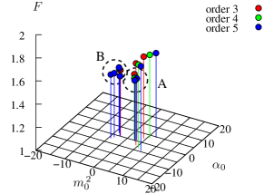
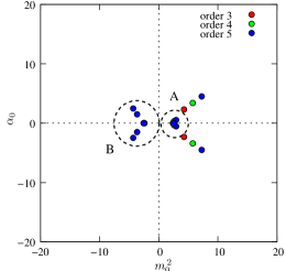
  Figure 1: Distribution of extrema of $F^{\text{imp}}(\alpha,m^{2};\alpha_{0},m_{0}^{2})$ with respect to $m_{0}^{2}$ and $\alpha_{0}$ at $\alpha=0.0$ and $m^{2}=0.0$. Vertical lines indicate the value of $F^{\text{imp}}$ at the extrema 1, and its 2-d plot in $(m_{0}^{2},\alpha_{0})$-plane 1.

  This corresponds to the pure Yang-Mills matrix model only with the four-point interaction terms.

  The distribution of extrema of $F^{\text{imp}}(\alpha_{0},m_{0}^{2})$ with respect to $m_{0}^{2}$, $\alpha_{0}$ and its value at each extremum are shown in Fig. 1. We can find two accumulations of extrema as shown by the dashed circles A, B. These two accumulations also appear for $A^{\text{imp}}(\alpha_{0},m_{0}^{2})$ and the improved series for the expectation value of the second moment of eigenvalues

  $$C(\alpha,m^{2})\equiv\frac{1}{3}\sum_{\mu}\left\langle\frac{1}{N}{\rm tr}\left(A_{\mu}^{2}\right)\right\rangle.$$ (32)

  Except for these accumulations, there are gentle plateaux in the regions where the value of $|m_{0}^{\,2}|$ is very large. However, we do not take into account these flat regions as plateaux because these are nothing but asymptotic behaviors. These asymptotic behaviors always appear and we neglect them hereafter. By comparing the values of the improved free energy, we regard the plateau of region A as the true vacuum. The concrete values of the extrema and those of $F^{\text{imp}}(\alpha_{0},m_{0}^{2})$ there are listed in Table 1, and those for $A^{\text{imp}}(\alpha_{0},m_{0}^{2})$ are listed in Table 2. Because $A^{\text{imp}}$ is zero (Table 2), this vacuum can be recognized as the Yang-Mills vacuum.

  Thus this parameter region corresponds to the Yang-Mills phase.

• $(\alpha,m^{2})=(10.0,0.0)$

  

  

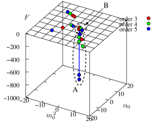
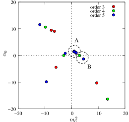
  Figure 2: Distribution of extrema of $F^{\text{imp}}(10.0,0.0;\alpha_{0},m_{0}^{2})$ with respect to $m_{0}^{2}$ and $\alpha_{0}$. Vertical lines indicate the value of $F^{\text{imp}}$ at the extrema 2, and its 2-d plot in $(m_{0}^{2},\alpha_{0})$-plane 2.

  The distribution of extrema of $F^{\text{imp}}(\alpha_{0},m_{0}^{2})$ with respect to $m_{0}$, $\alpha_{0}$ and its value at each extremum are shown in Fig. 2. From the Fig. 2 we find an accumulation of extrema. We point out that this accumulation is divided into two sets A and B by examining $F^{\text{imp}}$. As for the region A, the values of $F^{\text{imp}}$ at extrema go to large negative values as the order increases. On the other hand the values of $F^{\text{imp}}$ at extrema in the region B remain $\mathcal{O}(1)$. They also appear for $A^{\text{imp}}$. The concrete values of the extrema and those of $F^{\text{imp}}(\alpha_{0},m_{0}^{2})$ there are listed in Table 3, and those for $A^{\text{imp}}(\alpha_{0},m_{0}^{2})$ are listed in Table 4.

  One might think that the region A cannot be regarded as a plateau because the values of $F^{\text{imp}}$ are not stable against the increase of the order (Fig. 2). These values are all beyond $\mathcal{O}(1)$ and in particular, the values of $F^{\text{imp}}$ and $A^{\text{imp}}$ at the fifth order reach to about $\mathcal{O}(10^{3})$ and $\mathcal{O}(10^{4})$, respectively, as shown in Table 3 and Table 4. In general the improved perturbation theory is an approximation by polynomials of finite order and therefore the value of $\mathcal{O}(N^{2})$ which goes infinite as $N\to\infty$ is expected to be approximated as large amount of value. As we go to higher orders, the approximation would become better and would provide a larger value in such a case. In this sense, instability of an approximated value against an increase of order is not always problematic. Thus we identify the region A as a plateau. By comparing the values of $F^{\text{imp}}$ in the region A and B we regard the plateau of the region A as the true vacuum.

  Because the value of $A^{\text{imp}}$ in this plateau is $\mathcal{O}(10^{4})$ (Table 4), this vacuum can be recognized as the fuzzy sphere vacuum and this parameter region corresponds to the fuzzy sphere phase.

• $(\alpha,m^{2})=(4.0,1.5)$

  

  

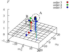
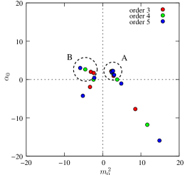
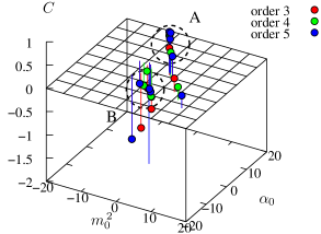
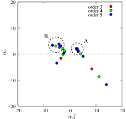
  Figure 3: Distribution of extrema of $F^{\text{imp}}(4.0,1.5;\alpha_{0},m_{0}^{2})$ with respect to $m_{0}^{2}$ and $\alpha_{0}$. Vertical lines indicate the value of $F^{\text{imp}}$ at the extrema 3, and its 2-d plot in $(m_{0}^{2},\alpha_{0})$-plane 3.

  

  

  Figure 4: Distribution of extrema of $C^{\text{imp}}(4.0,1.5;\alpha_{0},m_{0}^{2})$ with respect to $m_{0}^{2}$ and $\alpha_{0}$. Vertical lines indicate the value of $C^{\text{imp}}$ at the extrema 4, and its 2-d plot in $(m_{0}^{2},\alpha_{0})$-plane 4.

  The distribution of extrema of $F^{\text{imp}}(\alpha_{0},m_{0}^{2})$ with respect to $m_{0}$, $\alpha_{0}$ and its value at each extremum are shown in Fig. 3. We can find two accumulations of extrema. They also appear for $A^{\text{imp}}$. By comparing the values of $F^{\text{imp}}$, the region B is expected as the true vacuum. However the values of $C^{\text{imp}}$ at extrema in this plateau become negative (Fig. 4). Thus we determine this plateau is unphysical. Then the plateau in the region A is recognized as the true vacuum which has negative $\mathcal{O}(1)$ values of $F^{\text{imp}}$ and $A^{\text{imp}}$. The concrete values of the extrema and those of $F^{\text{imp}}(\alpha_{0},m_{0}^{2})$, $C^{\text{imp}}(\alpha_{0},m_{0}^{2})$, and $A^{\text{imp}}(\alpha_{0},m_{0}^{2})$ are listed in Table 5, 6, and 7, respectively.

  Because the value of $A^{\text{imp}}$ in the region A is negative $\mathcal{O}(1)$ value (Table 7) this parameter region corresponds to the 5-brane phase.

• $(\alpha,m^{2})=(2.0,10.0)$

  

  

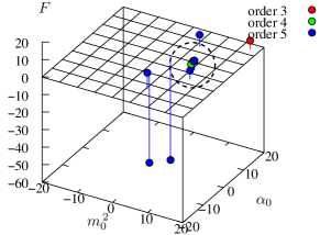
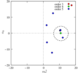
  Figure 5: Distribution of extrema of $F^{\text{imp}}(2.0,10.0;\alpha_{0},m_{0}^{2})$ with respect to $m_{0}^{2}$ and $\alpha_{0}$. Vertical lines indicate the value of $F^{\text{imp}}$ at the extrema 5, and its 2-d plot in $(m_{0}^{2},\alpha_{0})$-plane 5.

  The distribution of extrema of $F^{\text{imp}}(\alpha_{0},m_{0}^{2})$ with respect to $m_{0}$, $\alpha_{0}$ and its value at each extremum are shown in Fig. 5. We can find an accumulation of extrema. The concrete values of the extrema and those of $F^{\text{imp}}(\alpha_{0},m_{0}^{2})$ there are listed in Table 8, and those for $A^{\text{imp}}(\alpha_{0},m_{0}^{2})$ are listed in Table 9.

  Because the value of $A^{\text{imp}}$ in this plateau is around zero (Table 9), this vacuum corresponds to the Yang-Mills vacuum. Thus this parameter region corresponds to the Yang-Mills phase.

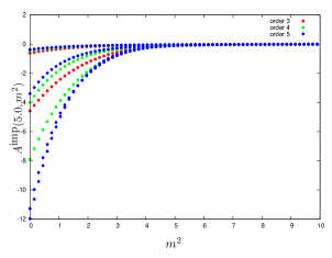
Now we proceed to discussion in the case of generic $\alpha$ and $m^{2}$. As an illustration we plot the values of $F^{\text{imp}}$ and $A^{\text{imp}}$ at their extrema with positive $m_{0}^{2}$ as functions of $\alpha$ when $m^{2}$ is zero (Fig. 6 and Fig. 7). From these figures we can divide the set of extrema into two branches: one branch consists of extrema for which the values of $F^{\text{imp}}$ and $A^{\text{imp}}$ remain of $\mathcal{O}(1)$ against the increase of $\alpha$, while the other branch is composed of extrema for which the values of $F^{\text{imp}}$ and $A^{\text{imp}}$ decrease far more than of $\mathcal{O}(10)$ as $\alpha$ increases. This property can be seen clearly in Fig. 7. We call the former as branch B and the latter as branch A. In fact each branch corresponds to an accumulation of extrema in $(\alpha_{0},m_{0}^{2})$-plane. The branch A, B corresponds to the plateau of the region A, B respectively at the above mentioned case $(\alpha,m^{2})=(10.0,0.0)$. These two branches join together for small $\alpha$, and thus we find only one accumulation at $(\alpha,m^{2})=(0.0,0.0)$.

Figure 6: Values of $F^{\text{imp}}(\alpha,0.0;\alpha_{0},m_{0}^{2})$ at extrema as functions of $\alpha$.

Figure 7: Values of $A^{\text{imp}}(\alpha,0.0;\alpha_{0},m_{0}^{2})$ at extrema 7 and its absolute value in logarithmic scale 7 as functions of $\alpha$.

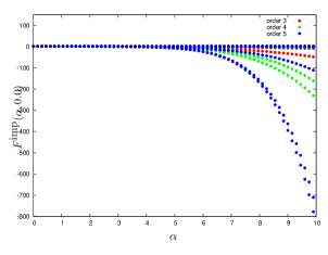
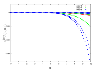
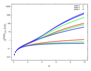
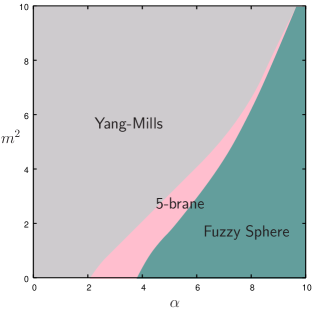
By comparing the values of $F^{\text{imp}}$ (Fig. 6), we identify the plateau corresponding to the branch A as the true vacuum as in the case of $(\alpha,m^{2})=(10.0,0.0)$. We take the expectation value of the Chern-Simons term as an order parameter. By examining the value of $A^{\text{imp}}$ in this branch we can determine what phase appears at each $(\alpha,m^{2})$. If it takes a value of $\mathcal{O}(N^{2})$, of $\mathcal{O}(1)$, and around zero, it corresponds to the fuzzy sphere phase, 5-brane phase, and Yang-Mills phase, respectively. Thus from Fig. 7 we conclude that there is the Yang-Mills phase in the region $0<\alpha<2$, the 5-brane phase in the region $2<\alpha<4$ and the fuzzy sphere phase in the region $\alpha>4$. We also note that if the set of extrema is divided into branches, it indicates that the behavior of the improved series and the distribution of extrema change drastically there. Then this would imply a phase transition there as mentioned in the beginning of this section. In fact, Fig. 7 shows this is the case with our model, namely around the phase transition points we can observe the branching of the extrema.

In the same manner, we observe the behavior of the value at extrema of $A^{\text{imp}}$ along an arbitrary path in $(\alpha,m^{2})$-plane. As an example, we show values of $A^{\text{imp}}(\alpha,m^{2};\alpha_{0},\alpha_{0}^{2})$ at extrema as functions of $m^{2}$ when $\alpha=5.0$ in Fig. 8.

Figure 8: Values of $A^{\text{imp}}(5.0,m^{2};\alpha_{0},m_{0}^{2})$ at extrema as functions of $m^{2}$.

From these investigations we can obtain a phase diagram of the massive YMCS matrix model in $(\alpha,m^{2})$-plane (Fig 9).

Figure 9: A proposed phase diagram of the massive Yang-Mills Chern-Simons matrix model.

VI Conclusions and Discussions

In this paper we applied the improved perturbation theory to the massive YMCS matrix model and calculated the free energy, and the expectation values of the second moment of eigenvalues and the Chern-Simons term up to the fifth order. Though the original perturbative series was obtained about the perturbative vacuum corresponding to the Yang-Mills vacuum, the improved perturbation theory reveals the information on the different vacua, namely the 5-brane vacuum and the fuzzy sphere vacuum.

As a result, we obtained the phase diagram of this model. The results are very similar to the previous work based on the one-loop calculation around the fuzzy sphere type background. Since the improved perturbation theory is expected to include nonperturbative effects, we can expect that a gauge symmetry is generated as a subgroup of the original ${\it U}(N)$ group even nonperturbatively in the 5-brane phase and the fuzzy sphere phase. In particular, dynamical generation of a non-Abelian gauge group occurs nonperturbatively in the 5-brane phase. However the precise positions of the critical lines in our phase diagram are somewhat ambiguous. For example, in our phase diagram there exists the 5-brane phase for $2<\alpha<4$ when $m^{2}=0$, which apparently contradicts with the Monte Carlo result in Ref. Azuma:2004zq . This is because our improved perturbative series is constructed from the standard perturbative series of lower order. It is obvious that in order to observe the phase transition clearly, a lower order analysis is not sufficient. As we proceed to higher orders, this ambiguity would decrease and we would find the phase transitions between the three phases more precisely. Then a precise comparison to the phase diagram proposed in Ref. Azuma:2005bj makes sense and we can discuss to what extent the perturbative analysis is valid in various parameter regions.

Another result of this paper is a confirmation of validity of the improved perturbation theory. It is accomplished by comparing our result in Fig. 7 with the precedent result of the Monte Carlo method Azuma:2004yg . Although we can not see clearly the first-order phase transition between the Yang-Mills phase and the fuzzy sphere phase, our result indicates a similar parameter region ($\alpha_{critical}\sim\mathcal{O}(1)$) as a critical point to that of the Monte Carlo method.

It is worthwhile to mention the accumulation which was regarded as an unphysical plateau when $(\alpha,m^{2})=(4.0,1.5)$. This accumulation of the extrema shows the lower value of the free energy than that of the other plateau. Therefore it would be the true vacuum if it corresponds to a physical state. It is interesting that it has a positive expectation value of the Chern-Simons term which is an opposite sign compared to that in the usual 5-brane or fuzzy sphere vacuum. We considered this plateau unphysical because the expectation value of the second moment of eigenvalues is negative there. However if it becomes positive when we go to a higher order or relax the ${\it SO}(3)$-symmetric assumption (27), then we would have a nontrivial phase and the phase diagram would change. We leave it to a future work.

order	$\alpha_{0}$	$m_{0}^{\,2}$	$F^{\text{imp}}$
3	$-4.68729\times 10^{9}$	$-8.30606\times 10^{7}$	$26.1027$
	$4.68729\times 10^{9}$	$-8.30606\times 10^{7}$	$26.1027$
	$0.0$	$-2.40953$	$1.5702$
	$0.0$	$2.40953$	$1.5702$
	$-2.31723$	$4.29037$	$1.70658$
	$2.31723$	$4.29037$	$1.70658$
4	$0.341271$	$2.59243$	$1.54085$
	$-0.341271$	$2.59243$	$1.54085$
	$3.40785$	$5.75606$	$1.71942$
	$-3.40785$	$5.75606$	$1.71942$
5	$-2.46938$	$-4.30854$	$1.54941$
	$2.46938$	$-4.30854$	$1.54941$
	$-1.49032$	$-3.65313$	$1.55424$
	$1.49032$	$-3.65313$	$1.55424$
	$0.0$	$-2.54153$	$1.51756$
	$0.0$	$2.54153$	$1.51756$
	$-0.524011$	$2.9491$	$1.5305$
	$0.524011$	$2.9491$	$1.5305$
	$-4.51448$	$7.27529$	$1.73146$
	$4.51448$	$7.27529$	$1.73146$

Table 1: The numerical data of extrema for $F^{\text{imp}}(0.0,0.0;\alpha_{0},m_{0}^{2})$

order	$\alpha_{0}$	$m_{0}^{\,2}$	$A^{\text{imp}}$
3	$0.0$	$-3.08221$	$0.0$
	$-0.138803$	$-2.94881$	$0.000320748$
	$0.138803$	$-2.94881$	$-0.000320748$
	$0.0$	$-2.82843$	$0.0$
	$0.0$	$2.82843$	$0.0$
	$0.0$	$3.08221$	$0.0$
4	$5.45504$	$-6.42054$	$0.116302$
	$-5.45504$	$-6.42054$	$-0.116302$
	$0.0$	$-3.7272$	$0.0$
	$-0.290656$	$-3.458$	$0.000734582$
	$0.290656$	$-3.458$	$-0.000734582$
	$0.629447$	$-3.26122$	$0.000832601$
	$-0.629447$	$-3.26122$	$-0.000832601$
	$0.0$	$-3.24237$	$0.0$
	$0.270866$	$-2.89579$	$0.00388426$
	$-0.270866$	$-2.89579$	$-0.00388426$
	$0.0$	$-2.66364$	$0.0$
	$0.0$	$2.66364$	$0.0$
	$0.0$	$3.24237$	$0.0$
	$0.0$	$3.7272$	$0.0$
5	$0.0$	$-4.42101$	$0.0$
	$0.445076$	$-4.03236$	$-0.000992029$
	$-0.445076$	$-4.03236$	$0.000992029$
	$0.0$	$-3.75696$	$0.0$
	$0.965698$	$-3.72636$	$0.000171623$
	$-0.965698$	$-3.72636$	$-0.000171623$
	$-1.00261$	$-3.69771$	$-0.000168316$
	$1.00261$	$-3.69771$	$0.000168316$
	$0.0787589$	$2.77319$	$-0.000243519$
	$-0.0787589$	$2.77319$	$0.000243519$
	$0.0$	$3.75696$	$0.0$
	$0.0$	$4.42101$	$0.0$

Table 2: The numerical data of extrema for $A^{\text{imp}}(0.0,0.0;\alpha_{0},m_{0}^{2})$

order	$\alpha_{0}$	$m_{0}^{\,2}$	$F^{\text{imp}}$
3	$9.43649$	$-7.60688$	$3.07945$
	$9.04356$	$-6.42828$	$3.06715$
	$-4.43165$	$-5.84631$	$1.67693$
	$1.43896$	$0.862241$	$-49.4706$
	$0.876274$	$1.6869$	$-9.32175$
	$-10.2822$	$9.45705$	$2.64061$
4	$10.5828$	$-9.79928$	$3.08573$
	$-0.00542322$	$-2.96341$	$7.73904$
	$1.53846$	$0.937571$	$-243.211$
	$1.32581$	$1.08363$	$-169.926$
	$0.00542358$	$2.95278$	$-4.62466$
	$-16.3116$	$13.527$	$2.75701$
5	$11.5522$	$-11.9498$	$3.08677$
	$-9.84509$	$-9.44094$	$1.5811$
	$0.791191$	$-2.37935$	$-14.4279$
	$1.42496$	$0.986792$	$-762.155$
	$1.58502$	$1.01745$	$-835.662$
	$1.06366$	$1.73127$	$-116.83$
	$-1.32478$	$4.47375$	$-2.3464$
	$-22.4794$	$17.6733$	$2.82902$

Table 3: The numerical data of extrema for $F^{\text{imp}}(10.0,0.0;\alpha_{0},m_{0}^{2})$

order	$\alpha_{0}$	$m_{0}^{\,2}$	$A^{\text{imp}}$
3	$9.94959$	$-7.34049$	$0.0901421$
	$-0.00271556$	$-2.95803$	$1.23634$
	$1.40096$	$0.995306$	$-106.684$
	$0.00271758$	$2.95805$	$-1.23634$
4	$-22.1864$	$-15.5176$	$-0.0340077$
	$11.4184$	$-9.11834$	$0.0886916$
	$0.798254$	$-2.2225$	$-8.76388$
	$1.501$	$0.998731$	$-519.979$
	$1.12189$	$1.54166$	$-73.7818$
	$-1.65882$	$4.95124$	$-0.637283$
5	$12.4504$	$-10.8361$	$0.0890299$
	$8.65517$	$-6.44966$	$0.101811$
	$-1.90908$	$-4.94843$	$1.46692$
	$1.1106$	$-2.05508$	$40.6892$
	$1.51445$	$1.01601$	$-1385.51$
	$1.42806$	$1.18735$	$-1840.99$
	$0.703556$	$2.33845$	$-37.6504$
	$-3.67883$	$7.04633$	$-0.431045$

Table 4: The numerical data of extrema for $A^{\text{imp}}(10.0,0.0;\alpha_{0},m_{0}^{2})$

order	$\alpha_{0}$	$m_{0}^{\,2}$	$F^{\text{imp}}$
3	$9.61196\times 10^{10}$	$-6.49178\times 10^{7}$	$25.8232$
	$-5.7603\times 10^{9}$	$-4.47955\times 10^{6}$	$22.5561$
	$-1.92635$	$-3.3072$	$-0.277788$
	$2.01317$	$-3.09678$	$1.21161$
	$1.71943$	$-2.35192$	$1.1326$
	$2.17535$	$2.25552$	$1.94668$
	$0.966819$	$2.85037$	$2.20386$
	$-7.70211$	$8.53538$	$2.99592$
	$1.82382\times 10^{12}$	$1.63535\times 10^{8}$	$8.64457$
4	$2.66644$	$-4.5446$	$1.27361$
	$-0.00980172$	$-2.38145$	$1.97284$
	$1.7947$	$2.42488$	$1.90002$
	$2.27369$	$2.50761$	$1.86237$
	$0.0104127$	$3.78695$	$2.27765$
	$-11.785$	$11.6617$	$3.04714$
5	$3.01798$	$-5.86682$	$1.29304$
	$-4.23407$	$-5.18175$	$-0.613976$
	$0.45086$	$-2.18319$	$-0.0677834$
	$2.00342$	$2.38336$	$1.82213$
	$2.2562$	$2.7082$	$1.82699$
	$1.20384$	$2.99017$	$1.95765$
	$-1.03239$	$4.86228$	$2.3355$
	$-15.9168$	$14.8553$	$3.08096$

Table 5: The numerical data of extrema for $F^{\text{imp}}(4.0,1.5;\alpha_{0},m_{0}^{2})$

order	$\alpha_{0}$	$m_{0}^{\,2}$	$C^{\text{imp}}$
3	$3.39189$	$-6.74048$	$-0.48585$
	$-3.47241$	$-5.02842$	$-1.38562$
	$3.80442$	$-4.2263$	$-0.560315$
	$2.58809$	$-4.03884$	$-0.497245$
	$3.1278$	$-3.50164$	$-0.581923$
	$-1.621$	$-3.47036$	$-1.18014$
	$1.0354$	$-2.03806$	$-0.841414$
	$2.12207$	$2.47803$	$0.786263$
	$2.04249$	$2.50236$	$0.873765$
	$2.07634$	$2.85198$	$0.859968$
	$0.919071$	$3.14954$	$0.586119$
	$1.21074$	$3.2149$	$0.766484$
	$-0.859116$	$5.0785$	$0.514263$
	$-5.67532$	$8.38804$	$0.292278$
	$-11.7333$	$13.9904$	$0.273057$
	$3.87597\times 10^{12}$	$4.55414\times 10^{8}$	$1.73042\times 10^{-8}$
	$-4.05022\times 10^{12}$	$3.90586\times 10^{9}$	$0.0$
4	$3.07677$	$-5.41897$	$-0.488433$
	$2.0976$	$-2.75252$	$-0.626686$
	$-0.0734577$	$-2.68203$	$-0.00223366$
	$1.25144$	$-2.16141$	$-0.5948$
	$2.12631$	$2.58726$	$0.829878$
	$1.79011$	$2.68894$	$0.811098$
	$0.0567346$	$4.05283$	$0.54443$
	$-8.67938$	$11.1616$	$0.280595$
	$-2.06462\times 10^{11}$	$5.2415\times 10^{7}$	$1.0194\times 10^{-6}$
	$2.78288\times 10^{11}$	$7.59018\times 10^{7}$	$2.4174\times 10^{-7}$
5	$3.39189$	$-6.74048$	$-0.48585$
	$-3.47241$	$-5.02842$	$-1.38562$
	$3.80442$	$-4.2263$	$-0.560315$
	$3.1278$	$-3.50164$	$-0.581923$
	$0.330493$	$-2.35159$	$-2.49497$
	$2.04249$	$2.50236$	$0.873765$
	$2.07634$	$2.85198$	$0.859968$
	$1.21074$	$3.2149$	$0.766484$
	$-0.859116$	$5.0785$	$0.514263$
	$-11.7333$	$13.9904$	$0.273057$
	$-1.2577\times 10^{11}$	$4.10542\times 10^{7}$	$2.22914\times 10^{-6}$
	$5.85754\times 10^{11}$	$1.06032\times 10^{8}$	$1.83291\times 10^{-6}$

Table 6: The numerical data of extrema for $C^{\text{imp}}(4.0,1.5;\alpha_{0},m_{0}^{2})$

order	$\alpha_{0}$	$m_{0}^{\,2}$	$A^{\text{imp}}$
3	$2.34863$	$-2.98275$	$0.344616$
	$-0.00869776$	$-2.30156$	$1.30642$
	$1.98521$	$2.40399$	$-0.679792$
	$0.00529296$	$3.80166$	$-0.198496$
4	$-8.43836$	$-7.87598$	$-0.122983$
	$3.58394$	$-4.43987$	$0.312971$
	$0.553466$	$-2.13643$	$-0.541593$
	$2.11319$	$2.50874$	$-0.812064$
	$1.33838$	$2.85121$	$-0.576061$
	$-1.28207$	$5.19139$	$-0.156768$
5	$4.11377$	$-5.56741$	$0.310493$
	$-1.1206$	$-3.34363$	$2.1189$
	$0.722978$	$-2.04584$	$2.72295$
	$1.04265$	$-2.01922$	$0.734287$
	$2.08655$	$2.54758$	$-0.866595$
	$1.93161$	$2.68347$	$-0.877446$
	$0.744671$	$3.4634$	$-0.504538$
	$-2.62651$	$6.65831$	$-0.133145$

Table 7: The numerical data of extrema for $A^{\text{imp}}(4.0,1.5;\alpha_{0},m_{0}^{2})$

order	$\alpha_{0}$	$m_{0}^{\,2}$	$F^{\text{imp}}$
3	$1.64718$	$10.4191$	$4.97903$
	$17.4705$	$17.5462$	$4.99209$
	$-24.2305$	$20.3698$	$5.03619$
4	$1.91975$	$10.5121$	$4.97903$
	$0.00745054$	$10.8081$	$4.97907$
	$0.0074495$	$10.8081$	$4.97907$
	$26.7536$	$22.5472$	$5.00089$
	$-36.51$	$26.4821$	$5.05249$
5	$5.0158$	$2.06827$	$-59.5252$
	$-5.75065$	$2.28982$	$-50.2504$
	$-12.1958$	$5.41985$	$9.34926$
	$12.4862$	$6.04493$	$6.64019$
	$1.76262$	$10.5456$	$4.97903$
	$1.95766$	$10.6191$	$4.97903$
	$-2.77239$	$12.0802$	$4.97928$
	$35.9114$	$27.6808$	$5.00761$
	$-48.7488$	$32.7442$	$5.06396$

Table 8: The numerical data of extrema for $F^{\text{imp}}(2.0,10.0;\alpha_{0},m_{0}^{2})$

order	$\alpha_{0}$	$m_{0}^{\,2}$	$A^{\text{imp}}$
3	$0.566682$	$-0.941477$	$48.9325$
	$0.460771$	$-0.890109$	$48.8427$
	$-0.043734$	$-0.807144$	$68.646$
	$0.113023$	$-0.728224$	$58.1744$
	$1.92014$	$10.6554$	$-0.00337663$
	$0.00372349$	$10.8095$	$-0.00330928$
4	$-1.33655$	$-1.39229$	$-116.063$
	$-0.166586$	$-1.07679$	$202.618$
	$-0.458842$	$-0.94533$	$57.275$
	$0.131775$	$-0.934978$	$108.256$
	$-0.128625$	$-0.778924$	$-145.652$
	$0.257705$	$-0.733339$	$974.75$
	$0.12539$	$-0.674379$	$885.926$
	$1.83575$	$10.5838$	$-0.00337685$
	$1.90363$	$10.8436$	$-0.00337683$
	$-3.28575$	$12.5122$	$-0.00307347$
5	$1.08531$	$-1.82014$	$59.1655$
	$0.511521$	$-1.44973$	$41.398$
	$-0.271338$	$-1.42093$	$434.787$
	$0.174771$	$-1.23817$	$73.8638$
	$1.90812$	$10.5967$	$-0.00337686$
	$1.33656$	$10.6194$	$-0.0033768$
	$1.87274$	$11.0713$	$-0.00337686$
	$-6.75945$	$14.7516$	$-0.00278608$

Table 9: The numerical data of extrema for $A^{\text{imp}}(2.0,10.0;\alpha_{0},m_{0}^{2})$