Multidimensional Worldline Instantons

Abstract

We extend the worldline instanton technique to compute the vacuum pair production rate for spatially inhomogeneous electric background fields, with the spatial inhomogeneity being genuinely two or three dimensional, both for the magnitude and direction of the electric field. Other techniques, such as WKB, have not been applied to such higher dimensional problems. Our method exploits the instanton dominance of the worldline path integral expression for the effective action.

I Introduction

A remarkable prediction of quantum electrodynamics (QED) is that in the presence of an electric field the polarization of the vacuum can lead to the production of electron-positron pairs from vacuum. This was initially predicted and estimated for approximately uniform fields he ; schwinger , but has not yet been observed experimentally due to the extreme scales required greiner ; ringwald . In achieving such extreme field strengths, the inhomogeneity of the field becomes important. Much work has been done to estimate the pair production rate for electric fields whose direction is fixed and whose magnitude varies in one dimension, either spatial nikishov ; kimpage or temporal nikishov2 ; brezin ; popov . These approaches are semiclassical, essentially WKB or its variants. More recently, a Monte Carlo worldline loop method has been developed and applied to the vacuum pair production problem giesklingmuller . In principle, this Monte Carlo method can be applied to very general electric fields, but it has so far only been applied to the case of one-dimensional spatial inhomogeneities. The worldline instanton method, in which the Monte Carlo sum is effectively dominated by a single instanton loop, was introduced for constant fields in affleck , and extended to inhomogeneous fields in wli1 ; wli2 . For one-dimensional inhomogeneities, the agreement between WKB methods, worldline instantons and the Monte Carlo results is excellent wli2 . In this paper, we apply the worldline instanton method to electric fields with multidimensional inhomogeneities. Specifically, we compute the pair production rate for a class of spatially inhomogeneous electric fields, in which both the magnitude and direction of the electric field vary in two or three dimensional space. It is not clear how to compute the pair production rate for such fields using WKB.

The vacuum pair production rate can be deduced from the imaginary part of the effective action $\Gamma$ schwinger :

$$P_{\rm production}=1-e^{-2\,{\rm Im}\,\Gamma}\approx 2\,{\rm Im}\,\Gamma\quad.$$ (1.1)

The technical problem is thus to compute ${\rm Im}\,\Gamma$ for a given background electric field. This is nontrivial as the answer is non-perturbative in the field. For example, for a constant electric field the leading weak field result (for scalar QED) is

$$\frac{{\rm Im}\,\Gamma}{V_{4}}\sim\frac{e^{2}E^{2}}{16\pi^{3}}\,e^{-\frac{m^{2}\pi}{eE}}\quad.$$ (1.2)

For inhomogeneous fields, the simplest approximation is the “locally constant field” (LCF) approximation, in which one replaces the constant $E$ in (1.2) by $E(x)$, and integrates:

$${\rm Im}\,\Gamma^{\rm LCF}\sim\frac{e^{2}}{16\pi^{3}}\int d^{4}x\,\vec{E}^{2}(x)\,e^{-\frac{m^{2}\pi}{e|\vec{E}(x)|}}\quad.$$ (1.3)

In this paper we compute improved approximations to ${\rm Im}\,\Gamma$ using the worldline instanton method. In Sec.II, we review the worldline instanton method for computing the prefactor; in Sec. III, we present explicit computations of ${\rm Im}\,\Gamma$ for two-dimensional spatially inhomogeneous electric field backgrounds, and in Sec. IV, we present explicit computations of ${\rm Im}\,\Gamma$ for three-dimensional spatially inhomogeneous electric field backgrounds. We conclude with some brief comments on possible extensions.

II Worldine Instanton Method

The worldline formalism for QED provides a nonperturbative approach to computing $\Gamma$, and in particular its imaginary part. The worldline formalism expresses the one-loop effective action for a scalar charged particle (of charge $e$ and mass $m$) in a gauge background $A_{\mu}$ as a quantum mechanical path integral feynman ; halpern ; bern ; strassler ; csreview

$$\Gamma[A]=\int_{0}^{\infty}\frac{dT}{T}\,{\rm e}^{-m^{2}T}\int d^{4}x^{(0)}\!\!\!\!\!\!\!\int\limits_{x(T)=x(0)=x^{(0)}}\!\!\!\!\!\!\!\!\!\!{\mathcal{D}}x\,\,{\rm exp}\left[-\int_{0}^{T}d\tau\left(\frac{\dot{x}^{2}}{4}+ieA\cdot\dot{x}\right)\right].$$ (2.4)

Here the functional integral $\int{\mathcal{D}}x$ is over all closed Euclidean spacetime paths $x_{\mu}(\tau)$ that are periodic (with period $T$) in the proper-time parameter $\tau$. These closed paths are based at the marked point $x_{\mu}^{(0)}$, whose location is integrated over polyakov ; gerry . We use the path integral normalization conventions of csreview . The effective action $\Gamma[A]$ is a functional of the classical background field $A_{\mu}(x)$, which is a given function of the space-time coordinates.

The worldline instanton method is based on the observation affleck ; wli1 ; wli2 that for certain classical background fields the quantum mechanical path integral in (2.4) may be dominated by an instanton configuration, which is a closed path $x_{\mu}(\tau)$ satisfying the classical Euclidean equations of motion

$$\ddot{x}_{\mu}=2ie\,F_{\mu\nu}(x)\,\dot{x}_{\nu}\quad,\quad(\mu,\nu=1\dots 4)\quad,$$ (2.5)

where $F_{\mu\nu}=\partial_{\mu}A_{\nu}-\partial_{\nu}A_{\mu}$ is the background field strength. Worldline instantons are periodic solutions to (2.5). For uniform affleck and inhomogeneous wli1 background electric fields, these classical worldline instantons straightforwardly determine the nonperturbative exponential factor in ${\rm Im}\,\Gamma$.

However, this exponential factor is only part of the story. For inhomogeneous fields, the prefactor is also important. For example, with a spatially inhomogeneous electric field, there is a cutoff in the scale of the inhomogeneity, beyond which the pair production rate vanishes. Interestingly, this cutoff is reflected in the prefactor and not in the exponential factor giesklingmuller ; wli2 ; kimpage . Physically, this cutoff arises when the range of the electric field is so small that a virtual pair accelerated by the field does not acquire sufficient energy to become real particles.

To compute the prefactor one must compute the effect of the fluctuations about the classical worldline instanton path. The strategy for computing the prefactor was explained in wli2 . The basic idea is that the quantum mechanical path integral in (2.4) may be approximated as levit

$$\int\limits_{x(T)=x(0)=x^{(0)}}\!\!\!\!\!\!\!\!{\mathcal{D}}x\,\,{\rm exp}\left[-\int_{0}^{T}d\tau\left(\frac{\dot{x}^{2}}{4}+ieA\cdot\dot{x}\right)\right]\approx\frac{1}{(4\pi)^{2}}\frac{e^{-S[x^{\rm cl}](T)}}{\sqrt{{\rm Det}\,\Lambda}}\quad,$$ (2.6)

where $\Lambda$ is the operator describing quadratic fluctuations about the worldline instanton path:

$$\Lambda_{\mu\nu}\equiv-\frac{1}{2}\,\delta_{\mu\nu}\,\frac{d^{2}}{d\tau^{2}}+ie\,F_{\mu\nu}(x)\,\frac{d}{d\tau}+ie\,\partial_{\mu}F_{\nu\rho}(x)\,\dot{x_{\rho}}\quad.$$ (2.7)

An important technical observation levit ; kleinert is that ${\rm Det}\,\Lambda$ can be expressed as the determinant of a finite dimensional matrix, whose entries consist of certain solutions to the Jacobi equations,

$$\Lambda_{\mu\nu}\,\eta_{\nu}=0\quad,$$ (2.8)

evaluated at $\tau=T$. Specifically, we define the four independent solutions $\eta^{(\nu)}$ to (2.8), with initial value boundary conditions

$$\eta_{\mu}^{(\nu)}(0)=0\quad;\quad\dot{\eta}_{\mu}^{(\nu)}(0)=\delta_{\mu\nu}\quad.$$ (2.9)

Then levit ; kleinert

$${\rm Det}(\Lambda)={\rm det}\left[\eta_{\mu}^{(\nu)}(T)\right]\quad.$$ (2.10)

This provides a simple and general numerical method for computing the semiclassical approximation in (2.6), for a given proper-time $T$. The next step wli2 is to evaluate the remaining $T$ integral in (2.4) using steepest descents at a particular critical value $T_{c}$. This procedure was implemented explicitly in wli2 for inhomogeneous fields varying in one dimension, and the agreement with other computational methods was shown to be excellent. Here, in this paper, we extend this computational procedure explicitly to higher dimensional inhomogeneities.

II.1 Numerical method for finding worldline instanton loops

To be specific, we consider spatially inhomogeneous electric fields, $\vec{E}(\vec{x})$, for which we write the Euclidean gauge field as

$$A_{4}(\vec{x})=-i\frac{E}{k}\,f(k\vec{x})\quad.$$ (2.11)

Here $k$ is a parameter related to the scale of the variation of the function $f$. By analogy with Keldysh’s adiabaticity parameter keldysh for time dependent ionization problems, we define the dimensionless inhomogeneity parameter

$$\tilde{\gamma}=\frac{mk}{eE}\quad.$$ (2.12)

More general fields are characterized by many scale parameters, but the form in (2.11) is sufficient to illustrate our results.

The first numerical step is to find the closed worldline instanton path, as a periodic solution to the classical Euclidean equations of motions

$$\ddot{x}_{j} = 2eE\partial_{j}f\,\dot{x}_{4}\quad,\quad(j=1,2,3)\quad,$$ (2.13)

$$\ddot{x}_{4} = -2eE\partial_{j}f\,\dot{x}_{j}\quad.$$ (2.14)

To solve numerically these equations, we need to start from a point on the solution curve. In principle, this step can be done by a tedious search. However, for the cases considered in this paper, all the solutions pass through the local maximum of the electric field. Without loss of generality, we choose this point to be the origin: $\vec{x}=(0,0,0)$. We exploit the gauge freedom to choose $f(\vec{0})=0$.

Note that the $\ddot{x}_{4}$ equation (2.14) can be integrated immediately to yield

$$\dot{x}_{4}=-\frac{2eE}{k}f(k\vec{x})\quad,$$ (2.15)

where we have chosen the integration constant to vanish in order to have a periodic solution. Now, recall that (2.5) implies that $\dot{x}_{\mu}^{2}$ is constant on a classical solution:

$$\dot{x}_{\mu}^{2}=a^{2}\quad.$$ (2.16)

Thus, the magnitude, $|\dot{\vec{x}}(0)|$, of the “3-velocity” is equal to this constant $a$. But we do not know the initial direction of the 3-velocity. We use as shooting parameters the direction of the initial 3-velocity. For a one-dimensional problem where $f$ is a function of just one spatial coordinate, no shooting is required. For a two-dimensional problem where $f$ is a function of two spatial coordinates, one shooting parameter is required. For a three-dimensional problem where $f$ is a function of all three spatial coordinates, two shooting parameters are required. Given a value of the parameter $a$ in (2.16), we integrate the equations (2.13) and (2.14), adjusting the initial direction of the 3-velocity until a closed loop is found. The total proper-time $T$ required to close the loop is clearly a function of the parameter $a$, so

$$T=T(a)\quad{\rm or}\quad a=a(T)\quad.$$ (2.17)

For an electric field depending on two spatial coordinates, say $x_{1}$ and $x_{2}$, the loop has $\dot{x}_{3}=0$, and so depends in general on $x_{1}$, $x_{2}$ and $x_{4}$ only. An example of such a numerical worldline loop, for $f(kx_{1},kx_{2})=\frac{\tanh(kx_{1}+kx_{2})}{1+(kx_{1})^{2}+10(kx_{2})^{2}}$, is shown in Fig. 1.

Figure 1: Numerical worldline instanton loop for the case of $f(kx_{1},kx_{2})=\frac{\tanh(kx_{1}+kx_{2})}{1+(kx_{1})^{2}+10(kx_{2})^{2}}$. The first plot is the 3D parametrized plot of $\{x_{1}(\tau),x_{2}(\tau),x_{4}(\tau)\}$; the second plot is $x_{1}(\tau)$ vs. $x_{2}(\tau)$; the third plot is $x_{1}(\tau)$ vs. $x_{4}(\tau)$; and the last plot is $x_{2}(\tau)$ vs. $x_{4}(\tau)$. The parameters used to generate these plots are $E=1$, $k=\sqrt{2}$, $a=0.593$, and $\dot{x}_{1}(0)=0.562\,408\,091\,043\,522\,23$.

An example of such a numerical worldline loop for an electric field depending on all three spatial coordinates, with $f(kx_{1},kx_{2},kx_{3})=\frac{kx_{1}+kx_{2}+kx_{3}}{\left[1+(kx_{1})^{2}+2(kx_{2})^{2}+10(kx_{3})^{2}\right]^{2}}$, is shown in Fig. 2.

Figure 2: Numerical worldline instanton loop for the case of $f(kx_{1},kx_{2},kx_{3})=\frac{kx_{1}+kx_{2}+kx_{3}}{\left[1+(kx_{1})^{2}+2(kx_{2})^{2}+10(kx_{3})^{2}\right]^{2}}$. The first plot is the 3D parametrized plot of $\{x_{1}(\tau),x_{2}(\tau),x_{3}(\tau)\}$; the second plot is $\{x_{1}(\tau),x_{2}(\tau),x_{4}(\tau)\}$; the third plot is $\{x_{2}(\tau),x_{3}(\tau),x_{4}(\tau)\}$; and the last plot is $\{x_{3}(\tau),x_{1}(\tau),x_{4}(\tau)\}$. The parameters used to generate these plots are $E=1$, $k=1$, $\dot{x}_{1}(0)=0.6$, $\dot{x}_{2}(0)=0.453\,000\,684$, and $\dot{x}_{3}(0)=0.201\,733\,127\,28$.

This loop depends on all four space-time coordinates, so we plot appropriate cross-sections. Given these worldline loops, the pair production rate can be computed numerically as outlined above and in wli2 . In the following sections we illustrate this in some specific examples.

III Two-Dimensional Electric Fields

In this Section we illustrate our worldline instanton procedure in a class of models where the electric field is static and only depends on two spatial coordinates. For the 2D space-dependent fields of the form (2.11), the fluctuation operator (2.7) can be restricted to its components in the $(x_{1},x_{2},x_{4})$ plane :

$$\Lambda=\left(\begin{array}[]{ccc}-\frac{1}{2}\frac{d^{2}}{d^{2}\tau}+eEkf^{(2,0)}\dot{x}_{4}^{\rm cl}&eEkf^{(1,1)}\dot{x}_{4}^{\rm cl}&eEf^{(1,0)}\frac{d}{d\tau}\\ eEkf^{(1,1)}\dot{x}_{4}^{\rm cl}&-\frac{1}{2}\frac{d^{2}}{d^{2}\tau}+eEkf^{(0,2)}\dot{x}_{4}^{\rm cl}&eEf^{(0,1)}\frac{d}{d\tau}\\ -eE\frac{d}{d\tau}f^{(1,0)}&-eE\frac{d}{d\tau}f^{(0,1)}&-\frac{1}{2}\frac{d^{2}}{d^{2}\tau}\end{array}\right)\quad,$$ (3.18)

where

$$f^{(m,n)}\equiv\frac{\partial^{m}}{\partial z_{1}^{m}}\frac{\partial^{n}}{\partial z_{2}^{n}}f(z_{1},z_{2})\quad.$$ (3.19)

To compute the fluctuation determinant we use the semiclassical quantum mechanical path integral result (2.10). Thus, we need to find solutions to the Jacobi equations $\Lambda\,\eta=0$ in (2.8), satisfying the initial value conditions (2.9). In general, this needs to be done numerically. However, there exists a class of fields for which the entire computation can be done semi-analytically, providing more insight. Consider fields (2.11) with the symmetry

$$f(kx_{1},kx_{2})=f(kx_{2},kx_{1})\quad.$$ (3.20)

For example, the two-dimensional symmetric electric field example with $f(kx_{1},kx_{2})=(kx_{1}+kx_{2}){\rm e}^{-(kx_{1})^{2}-(kx_{2})^{2}}$, is shown in Fig. 3.

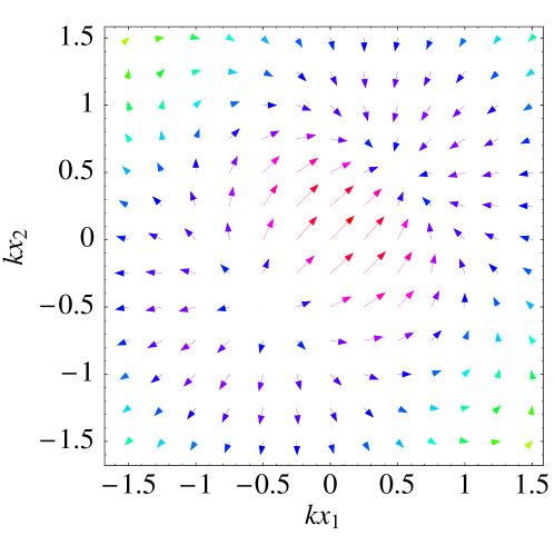
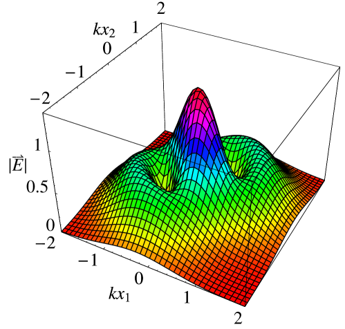
Figure 3: The electric field $\vec{E}(x_{1},x_{2})$ for the case of $f(kx_{1},kx_{2})=(kx_{1}+kx_{2}){\rm e}^{-(kx_{1})^{2}-(kx_{2})^{2}}$. The first plot is the vector plot of $\vec{E}$ as a function of $(kx_{1},kx_{2})$; the second plot is the 3D plot of the magnitude of $\vec{E}$ as a function of $(kx_{1},kx_{2})$. To generate these plots, we use the parameter $E=1$.

As can be seen from the Figure, such an electric field is genuinely two dimensional in its inhomogeneity, both for its direction and its magnitude. Physically, we choose the form of $f$ so that the electric field is spatially localized. Interestingly, for such fields the worldline instanton loop, which is a closed loop in three dimensions [$x_{1}$, $x_{2}$, and $x_{4}$], is planar. This implies that much of the analysis can be reduced to the one dimensional case studied in wli2 . Note, however, that even though the classical loop is essentially 2D, the fluctuations extend non-trivially into the third direction.

III.1 Determinant of the Fluctuation Operator

We write the solution of the Jacobi equation $\Lambda\phi=0$ as

$$\phi=\left(\begin{array}[]{c}\phi_{1}\\ \phi_{2}\\ \phi_{4}\end{array}\right)\quad.$$ (3.21)

Numerically, one simply integrates the Jacobi equations with the initial value conditions (2.9). However, we can partially construct these solutions analytically, as follows. There are six linearly independent solutions, from which we need to construct the three independent solutions satisfying the initial conditions (2.9). To find all six linearly independent solutions, we use two different Ansätze:

1. $\phi_{1}=\phi_{2}$. In this case, the Jacobi equation reduces to

   $$-{\textstyle\frac{1}{2}}\ddot{\phi}_{1}+eEk\left[f^{(2,0)}+f^{(1,1)}\right]\dot{x}_{4}^{\rm cl}\phi_{1}+eEf^{(1,0)}\dot{\phi}_{4}=0\quad,$$

   $$\dot{\phi}_{4}=-4eEf^{(1,0)}\phi_{1}+v_{4}\quad,$$ (3.22)

   where $v_{4}$ is an integration constant. There are four independent solutions of this type. As in the 1D case considered in wli2 , we can write these four solutions as :

   $$\phi^{(1)}(\tau) = \left(\begin{array}[]{c}0\\ 0\\ 1\end{array}\right)\quad,\qquad\phi^{(2)}(\tau)=\left(\begin{array}[]{c}\dot{x}_{1}^{\rm cl}(\tau)\\ \dot{x}_{1}^{\rm cl}(\tau)\\ \dot{x}_{4}^{\rm cl}(\tau)\end{array}\right)\quad,$$ (3.29)

   $$\phi^{(3)}(\tau) = \left(\begin{array}[]{c}\dot{x}_{1}^{\rm cl}(t)\int_{0}^{\tau}dt\,\frac{1}{\left[\dot{x}_{1}^{\rm cl}(t)\right]^{2}}\\ \dot{x}_{1}^{\rm cl}(t)\int_{0}^{\tau}dt\,\frac{1}{\left[\dot{x}_{1}^{\rm cl}(t)\right]^{2}}\\ \dot{x}_{4}^{\rm cl}(\tau)\int_{0}^{\tau}dt\,\frac{1}{\left[\dot{x}_{1}^{\rm cl}(t)\right]^{2}}-\int_{0}^{\tau}dt\,\frac{\dot{x}_{4}^{\rm cl}(t)}{\left[\dot{x}_{1}^{\rm cl}(t)\right]^{2}}\end{array}\right)\quad,$$ (3.33)

   $$\phi^{(4)}(\tau) = \left(\begin{array}[]{c}\dot{x}_{1}^{\rm cl}(\tau)\int_{0}^{\tau}dt\,\frac{\dot{x}_{4}^{\rm cl}(t)}{\left[\dot{x}_{1}^{\rm cl}(t)\right]^{2}}\\ \dot{x}_{1}^{\rm cl}(\tau)\int_{0}^{\tau}dt\,\frac{\dot{x}_{4}^{\rm cl}(t)}{\left[\dot{x}_{1}^{\rm cl}(t)\right]^{2}}\\ \dot{x}_{4}^{\rm cl}(\tau)\int_{0}^{\tau}dt\,\frac{\dot{x}_{4}^{\rm cl}(t)}{\left[\dot{x}_{1}^{\rm cl}(t)\right]^{2}}-a^{2}\int_{0}^{\tau}dt\,\frac{1}{\left[\dot{x}_{1}^{\rm cl}(t)\right]^{2}}\end{array}\right)\quad.$$ (3.37)

2. $\phi_{1}=-\phi_{2}$, and $\phi_{4}=0$. In this case, the Jacobi equation reduces to a single second order differential equation:

   $$-{\textstyle\frac{1}{2}}\ddot{\phi}_{1}+eEk\left[f^{(2,0)}-f^{(1,1)}\right]\dot{x}_{4}^{\rm cl}\phi_{1}=0\quad.$$ (3.38)

   There are two independent solutions of this type. These are new to the two-dimensional case. Denote as $\psi^{(5)}$ and $\psi^{(6)}$ the two linearly independent solutions of (3.38) with the initial conditions:

   $$\psi^{(5)}(0)=1\quad, \dot{\psi}^{(5)}(0)=0\quad,$$

   $$\psi^{(6)}(0)=0\quad, \dot{\psi}^{(6)}(0)=1\quad.$$ (3.39)

   Then, we can write the last two solutions of the Jacobi solutions $\Lambda\phi=0$ as

   $$\phi^{(5)}(\tau)=\left(\begin{array}[]{c}\psi^{(5)}\\ -\psi^{(5)}\\ 0\end{array}\right)\quad,\qquad\phi^{(6)}(\tau)=\left(\begin{array}[]{c}\psi^{(6)}\\ -\psi^{(6)}\\ 0\end{array}\right)\quad.$$ (3.40)

Finally, given these six linearly independent solutions, $\phi^{(1)},\dots,\phi^{(6)}$, we construct the linear combinations satisfying the initial conditions (2.9) as

$$\eta^{(1)}(\tau) = {\textstyle\frac{1}{2}}\dot{x}_{1}^{\rm cl}(0)\phi^{(3)}(\tau)+{\textstyle\frac{1}{2}}\phi^{(6)}(\tau)\quad,$$

$$\eta^{(2)}(\tau) = {\textstyle\frac{1}{2}}\dot{x}_{1}^{\rm cl}(0)\phi^{(3)}(\tau)-{\textstyle\frac{1}{2}}\phi^{(6)}(\tau)\quad,$$

$$\eta^{(4)}(\tau) = {\textstyle\frac{1}{2}}\dot{x}_{4}^{\rm cl}(0)\phi^{(3)}(\tau)-{\textstyle\frac{1}{2}}\phi^{(4)}(\tau)\quad.$$ (3.41)

A lengthy but straightforward computation shows that the fluctuation determinant (2.10) takes the following simple form:

$$\mbox{Det}(\Lambda) = T\det\left[\eta^{(1)}(T),\,\eta^{(2)}(T),\,\eta^{(4)}(T)\right]$$ (3.42)

$$= \frac{T}{2}\frac{\left[\dot{x}_{1}^{\rm cl}(0)\right]^{3}}{\dot{x}_{1}^{\rm cl}(T)}\psi^{(6)}(T)\left[a^{2}I_{1}^{2}(T)-I_{2}^{2}(T)\right]\quad.$$

Here, $I_{1}(T)$ and $I_{2}(T)$ are integrals defined in terms of the closed worldline instanton loop:

$$I_{1}(\tau) \equiv \frac{\dot{x}_{1}^{\rm cl}(\tau)}{\dot{x}_{1}^{\rm cl}(0)}\,\int_{0}^{\tau}dt\,\frac{1}{\left[\dot{x}_{1}^{\rm cl}(t)\right]^{2}}\quad,$$

$$I_{2}(\tau) \equiv \frac{\dot{x}_{1}^{\rm cl}(\tau)}{\dot{x}_{1}^{\rm cl}(0)}\,\int_{0}^{\tau}dt\,\frac{\dot{x}_{4}^{\rm cl}(t)}{\left[\dot{x}_{1}^{\rm cl}(t)\right]^{2}}\quad.$$ (3.43)

The overall factor of $T$ is from the free $x_{3}$ direction levit .

The determinant (3.42) can be simplified further using periodicity, which implies that $\dot{x}_{1}^{\rm cl}(0)=\dot{x}_{1}^{\rm cl}(T)$, and the vanishing of $I_{2}(T)$. Therefore, we find the simple expression for the fluctuation determinant:

$$\mbox{Det}(\Lambda)=\frac{T}{2}\psi^{(6)}(T)\left[\frac{2eE}{k}\,\dot{x}_{1}^{\rm cl}(0)\,\bar{\gamma}(T)\,I_{1}(T)\right]^{2}\quad.$$ (3.44)

Here we have defined

$$\bar{\gamma}(T)\equiv\frac{k}{2eE}\,a(T)\quad.$$ (3.45)

Now recall from (2.4) and (2.6) that we still need to evaluate the $4$-dimensional space-time integral over the fixed point on the closed loops:

$$\int d^{4}x^{(0)} \equiv \int dx_{1}(0)\,dx_{2}(0)\,dx_{3}(0)\,dx_{4}(0)$$ (3.46)

$$= (L{\cal T})\int dx_{1}(0)\,dx_{2}(0)$$

$$= (L{\cal T})\frac{N}{k}\int d\tau\,\dot{x}_{1}^{\rm cl}(0)\quad,$$

where $L$ is the $1$-space volume and ${\cal T}$ is the total time. $N$ is a normalization factor that depends on the orientation of the loop. The simplest way to evaluate $N$ is to compare the $k\to 0$ limit with the corresponding locally constant field approximation answer (1.3), as explained below. Observe that the factor of $\dot{x}_{1}^{\rm cl}(0)$ appearing in (3.46) cancels against the same factor in $\sqrt{\mbox{Det}(\Lambda)}$ in (3.44), so that the spacetime integration effectively contributes a volume factor $(L{\cal T})$, a factor of $N/k$, and a factor of $\frac{T}{2}$ from the $\tau$ integral. This last factor is just the collective coordinate contribution arising from invariance under shifts of the starting point on the loop, which gives rise to the second of the zero modes in (3.37), as discussed in the 1D case in wli2 . Thus, collecting all the pieces, we see that the worldline instanton approximation (2.6) to the quantum mechanical path integral leads to :

$$\Gamma^{\rm WLI}\approx L{\cal T}\,\frac{N}{(4\pi)^{2}}\,\frac{\sqrt{2}}{4eE}\,\int_{0}^{\infty}\frac{dT}{\sqrt{T}}\,\frac{\exp\left[-\left(S[x^{\rm cl}](T)+m^{2}T\right)\right]}{\bar{\gamma}(T)I_{1}(T)\sqrt{\psi^{(6)}(T)}}\quad,$$ (3.47)

The main difference from the 1D case in wli2 is the appearance of the factor of $1/\sqrt{\psi^{(6)}(T)}$ and the power of $T$. The former is a measurement of the fluctuation in the second spatial direction; and the latter is because the remaining free dimension is now one instead of two.

III.2 The $T$ integral

As in wli2 , for spatially inhomogeneous electric fields we use a rotated steepest descents method to evaluate the $T$ integral in the vicinity of a critical point $T_{c}$. The critical point is a stationary point of the exponent in (3.47):

$$\Delta(T)\equiv S[x^{\rm cl}](T)+m^{2}T\quad.$$ (3.48)

This notation emphasizes the fact that the action $S[x^{\rm cl}]$, evaluated on the worldline instanton path $x^{\rm cl}(\tau)$, is a function of $T$. Near $T_{c}$, we have

$$\Delta(T)\approx\Delta(T_{c})+{\textstyle\frac{1}{2}}\Delta^{\prime\prime}(T_{c})(T-T_{c})^{2}+\cdots$$ (3.49)

As in the 1D cases, the critical point $T_{c}$ occurs when

$$\bar{\gamma}(T_{c})=\tilde{\gamma}\quad.$$ (3.50)

The rotation of the $T$ contour produces a factor of $i$, so our final expression is

$${\rm Im}\,\Gamma^{\rm WLI}\sim(L{\cal T})\,\frac{N}{32\pi^{3/2}}\,\frac{1}{eE}\,\frac{{\rm e}^{-\Delta(T_{c})}}{\tilde{\gamma}\,I_{1}(T_{c})\sqrt{T_{c}\,\psi^{(6)}(T_{c})|\Delta^{\prime\prime}(T_{c})|}}\quad.$$ (3.51)

III.3 Locally Constant Field Approximation

As in giesklingmuller ; wli2 ; kimpage , we compare the worldline instanton result with the locally constant field approximation (1.3). For example, consider the explicit example

$$f(kx_{1},kx_{2})=\frac{kx_{1}+kx_{2}}{1+(kx_{1})^{2}+(kx_{2})^{2}}\quad.$$ (3.52)

Expanding $|\vec{E}(x_{1},x_{2})|$ for small $k$, we find it is a quadratic function of a new pair of variables:

$$|\vec{E}(x_{1},x_{2})|\approx\sqrt{2}\,E\left(1-\frac{3}{2}k^{2}x_{+}^{2}-\frac{1}{2}k^{2}x_{-}^{2}+\cdots\right)\quad,$$ (3.53)

where $x_{+}\equiv x_{1}+x_{2}$, and $x_{-}\equiv x_{1}-x_{2}$. Thus, the leading LCF approximation is

$${\rm Im}\,\Gamma^{\rm LCF} \sim (L{\cal T})\frac{(eE)^{2}}{32\pi^{3}}\int dx_{+}\,dx_{-}\exp\left[-\frac{m^{2}\pi}{\sqrt{2}\,eE}\left(1+\frac{3}{2}k^{2}x_{+}^{2}+\frac{1}{2}k^{2}x_{-}^{2}\right)\right]\quad,$$ (3.54)

$$= (L{\cal T})\frac{(eE)^{3}}{4\sqrt{3}\,\pi^{3}(mk)^{2}}{\rm e}^{-\frac{m^{2}\pi}{\sqrt{2}\,eE}}\quad.$$

Comparing ${\rm Im}\,\Gamma^{\rm LCF}$ and the limiting value of ${\rm Im}\Gamma^{\rm WLI}$ as $k\to 0$, we find empirically that the normalization constant in (3.51) for the case of (3.52) is

$$N=2^{5/4}\frac{\sqrt{eE}}{m}\quad.$$ (3.55)

The same normalization factor arises for the exponentially localized field with $f(kx_{1},kx_{2})=(kx_{1}+kx_{2}){\rm e}^{-(kx_{1})^{2}-(kx_{2})^{2}}$. The ratio of the worldline instanton answer (3.51) to the LCF answer (3.54) is plotted in Fig. 4 for two different forms of the 2D electric field. In each case, there is a smooth dependence of the ratio from $1$ to $0$ as the inhomogeneity scale $\tilde{\gamma}$ [i.e. $k$] increases, which corresponds to the range of the field decreasing. Physically, the vanishing of the imaginary part at a critical inhomogeneity scale is because for very short range electric fields virtual dipole pairs do not acquire sufficient energy when accelerated in the field in order to become real particles. This has been observed previously for one dimensional spatial inhomogeneities giesklingmuller ; wli2 ; kimpage , and here we see it also in the higher dimensional case.

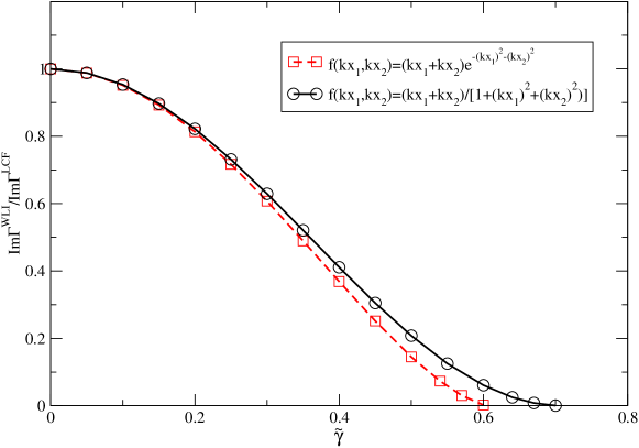
Figure 4: ${\rm Im}\,\Gamma^{\rm WLI}/{\rm Im}\,\Gamma^{\rm LCF}$ for the cases of $f(kx_{1},kx_{2})=\frac{kx_{1}+kx_{2}}{1+(kx_{1})^{2}+(kx_{2})^{2}}$, and $f(kx_{1},kx_{2})=(kx_{1}+kx_{2}){\rm e}^{-(kx_{1})^{2}-(kx_{2})^{2}}$. The parameters used to generate this plot are $E=1$, $e=1$, and $m=1$.

IV Three-Dimensional Electric Fields

For three dimensions the computation is very similar, with just a few changes. First, finding the worldline instanton loop requires a two parameter shooting procedure. Second, the fluctuation operator $\Lambda$ in (2.7) is now a $4\times 4$ matrix differential operator. The computation can be done numerically, but as in the 2D case we can gain more insight by specializing to a class of fields for which ${\rm Im}\,\Gamma$ can be computed semi-analytically. Consider totally symmetric fields (2.11) with

$$f(kx_{1},kx_{2},kx_{3})=f(kx_{2},kx_{1},kx_{3})=f(kx_{1},kx_{3},kx_{2})=f(kx_{3},kx_{2},kx_{1})\quad.$$ (4.56)

The electric field for an example with $f(kx_{1},kx_{2},kx_{3})=\frac{kx_{1}+kx_{2}+kx_{3}}{\left[1+(kx_{1})^{2}+(kx_{2})^{2}+(kx_{3})^{2}\right]^{3/2}}$ is shown in Fig. 5.

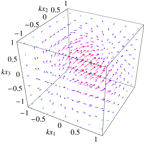
Figure 5: Vector plot of the electric field $\vec{E}(x_{1},x_{2},x_{3})$ for the case of $f(kx_{1},kx_{2},kx_{3})=\frac{kx_{1}+kx_{2}+kx_{3}}{\left[1+(kx_{1})^{2}+(kx_{2})^{2}+(kx_{3})^{2}\right]^{3/2}}$.

Note that it is localized, and that both the magnitude and direction of the field vary in three dimensions.

The calculation is similar to the two-dimensional symmetric case, except we now need eight [rather than six] independent solutions to the Jacobi equation, $\Lambda\phi=0$, in order to construct the four [rather than three] independent solutions $\eta^{(\nu)}$ satisfying the initial value conditions (2.9). In order to find the extra two solutions we extend the Ansätze for $\phi=(\phi_{1},\phi_{2},\phi_{3},\phi_{4})$ to:

1. Suppose $\phi_{1}=\phi_{2}=\phi_{3}$. Then $\Lambda\phi=0$ reduces to:

   $$-{\textstyle\frac{1}{2}}\ddot{\phi}_{1}+eEk\left[f^{(2,0,0)}+2f^{(1,1,0)}\right]\dot{x}_{4}^{\rm cl}\phi_{1}+eEkf^{(1,0,0)}\dot{\phi}_{4}=0\quad,$$

   $$\dot{\phi}_{4}=-6eEf^{(1,0,0)}\phi_{1}+v_{4}\quad.$$ (4.57)

   There are four solutions of this type. These solutions of the Jacobi equation are similar to those in the one- and two-dimensional cases.

2. Suppose $\phi_{1}=-\phi_{2}$ and $\phi_{3}=\phi_{4}=0$. In this case, the Jacobi equation reduces to a single second order differential equation, which is very similar to (3.38):

   $$-{\textstyle\frac{1}{2}}\ddot{\phi}_{1}+eEk\left[f^{(2,0,0)}-f^{(1,1,0)}\right]\dot{x}_{4}^{\rm cl}\phi_{1}=0\quad.$$ (4.58)

   There are two solutions of this type. Define $\psi^{(5)}$ and $\psi^{(6)}$ to be the solutions to (4.58) with the initial conditions in (3.39). Then two further solutions can be written as

   $$\phi^{(5)}(\tau)=\left(\begin{array}[]{c}\psi^{(5)}\\ -\psi^{(5)}\\ 0\\ 0\end{array}\right)\quad, \phi^{(6)}(\tau)=\left(\begin{array}[]{c}\psi^{(6)}\\ -\psi^{(6)}\\ 0\\ 0\end{array}\right)\quad.$$ (4.67)

3. Suppose $\phi_{1}=\phi_{2}=-{\textstyle\frac{1}{2}}\phi_{3}$, and $\phi_{4}=0$. In this case, the Jacobi equation reduces to exactly the same equation as in (4.58). There are two further solutions of this type. They can also be written in terms of $\psi^{(5)}$ and $\psi^{(6)}$:

   $$\phi^{(7)}(\tau)=\left(\begin{array}[]{c}\psi^{(5)}\\ \psi^{(5)}\\ -2\psi^{(5)}\\ 0\end{array}\right)\quad, \phi^{(8)}(\tau)=\left(\begin{array}[]{c}\psi^{(6)}\\ \psi^{(6)}\\ -2\psi^{(6)}\\ 0\end{array}\right)\quad.$$ (4.76)

Given these eight linearly independent solutions to $\Lambda\phi=0$, the linear combinations satisfying the initial conditions (2.9) are

$$\eta^{(1)}(\tau) = {\textstyle\frac{1}{3}}\dot{x}_{1}^{\rm cl}(0)\phi^{(3)}(\tau)+{\textstyle\frac{1}{2}}\phi^{(6)}(\tau)+{\textstyle\frac{1}{6}}\phi^{(8)}\quad,$$

$$\eta^{(2)}(\tau) = {\textstyle\frac{1}{3}}\dot{x}_{1}^{\rm cl}(0)\phi^{(3)}(\tau)-{\textstyle\frac{1}{2}}\phi^{(6)}(\tau)+{\textstyle\frac{1}{6}}\phi^{(8)}\quad,$$

$$\eta^{(3)}(\tau) = {\textstyle\frac{1}{3}}\dot{x}_{1}^{\rm cl}(0)\phi^{(3)}(\tau)-{\textstyle\frac{1}{3}}\phi^{(8)}(\tau)\quad,$$

$$\eta^{(4)}(\tau) = {\textstyle\frac{1}{3}}\dot{x}_{4}^{\rm cl}(0)\phi^{(3)}(\tau)-{\textstyle\frac{1}{3}}\phi^{(4)}(\tau)\quad.$$ (4.77)

A lengthy but straightforward computation shows that the fluctuation determinant (2.10) takes the simple form:

$$\mbox{Det}(\Lambda) = \det\left[\eta^{(1)}(T),\,\eta^{(2)}(T),\,\eta^{(3)}(T),\,\eta^{(4)}(T)\right]$$ (4.78)

$$= \frac{1}{3}\frac{\left[\dot{x}_{1}^{\rm cl}(0)\right]^{3}}{\dot{x}_{1}^{\rm cl}(T)}\left[\psi^{(6)}(T)\right]^{2}\left[a^{2}I_{1}^{2}(T)-I_{2}^{2}(T)\right]\quad,$$

where $I_{1}$ and $I_{2}$ are defined in (3.43). Notice the remarkable similarity to the 1D and 2D results for ${\rm Det}(\Lambda)$, in wli2 and (3.44), respectively.

Proceeding as in the 2D case, we find the following worldline instanton expression for the imaginary part of the effective action:

$${\rm Im}\,\Gamma^{\rm WLI}\sim{\cal T}\,\sqrt{\frac{3}{2}}\,\frac{N}{32\pi^{3/2}k}\,\frac{1}{eE}\frac{{\rm e}^{-\Delta(T_{c})}}{\tilde{\gamma}\,I_{1}(T_{c})\psi^{(6)}(T_{c})\,\sqrt{|\Delta^{\prime\prime}(T_{c})|}}\quad.$$ (4.79)

Here $N$ is a normalization constant coming from the spatial integrals, which depends on the form of the planar worldline instanton loop. As before, the simplest way to evaluate $N$ is by comparison of the $k\to 0$ limit of ${\rm Im}\,\Gamma^{\rm WLI}$ with the locally constant field approximation expression in (1.3). For example, for the case of $f(kx_{1},kx_{2},kx_{3})=(kx_{1}+kx_{2}+kx_{3}){\rm e}^{-(kx_{1})^{2}-(kx_{2})^{2}-(kx_{3})^{2}}$ we find

$${\rm Im}\,\Gamma^{\rm LCF}\sim{\cal T}\frac{3^{9/4}}{16\sqrt{7}}\,\frac{(eE)^{7/2}}{\pi^{3}(mk)^{3}}{\rm e}^{-\frac{m^{2}\pi}{\sqrt{3}eE}}\quad,$$ (4.80)

which leads to $N=\frac{9}{\sqrt{7}}\,\frac{eE}{m^{2}}$. And for the case of $f(kx_{1},kx_{2},kx_{3})=\frac{kx_{1}+kx_{2}+kx_{3}}{\left[1+(kx_{1})^{2}+(kx_{2})^{2}+(kx_{3})^{2}\right]^{3/2}}$ we find

$${\rm Im}\,\Gamma^{\rm LCF}\sim{\cal T}\frac{3^{3/4}}{4\sqrt{14}}\,\frac{(eE)^{7/2}}{\pi^{3}(mk)^{3}}{\rm e}^{-\frac{m^{2}\pi}{\sqrt{3}eE}}\quad,$$ (4.81)

and $N=\frac{6}{\sqrt{7}}\,\frac{eE}{m^{2}}$.

In Fig. 6 we plot as a function of the inhomogeneity scale $\tilde{\gamma}$, the ratio of the worldline instanton answer (4.79) to the LCF approximation answer (4.80) or (4.81), for these fields. Note once again that the pair production rate vanishes when the field becomes too closely localized.

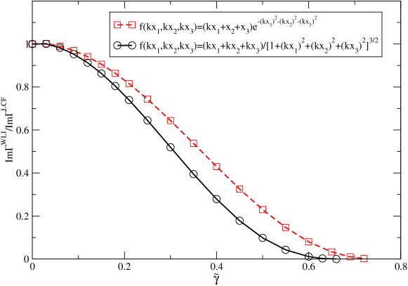
Figure 6: ${\rm Im}\,\Gamma^{\rm WLI}/{\rm Im}\,\Gamma^{\rm LCF}$ for the cases of $f(kx_{1},kx_{2},kx_{3})=\frac{kx_{1}+kx_{2}+kx_{3}}{\left[1+(kx_{1})^{2}+(kx_{2})^{2}+(kx_{3})^{2}\right]^{3/2}}$, and $f(kx_{1},kx_{2},kx_{3})=(kx_{1}+kx_{2}+kx_{3}){\rm e}^{-(kx_{1})^{2}-(kx_{2})^{2}-(kx_{3})^{2}}$. The parameters used to generate this plot are $E=1$, $e=1$, and $m=1$.

V Conclusions

In this paper we have extended the worldline instanton method of wli1 ; wli2 to the multi-dimensional case. Specifically, we have computed the imaginary part of the effective action in scalar QED for background electric fields that are inhomogeneous, both in their direction and magnitude, in two and three spatial dimensions. As in the one dimensional cases, the results exhibit the vanishing of the imaginary part when the inhomogeneity scale becomes too small, consistent with the physical picture of pair production as the acceleration of virtual dipole pairs in the electric field. In these multi-dimensional cases, there are currently no other computations with which to compare, except the crude locally constant field approximation, which does not capture the physics of the vanishing of ${\rm Im}\,\Gamma$ at short inhomogeneity scales. It would, however, be very interesting to compare with the numerical Monte Carlo worldline loop approach of Gies et al giesklingmuller , to see if the instanton dominance of the worldline instanton method can be combined with the versatility of the Monte Carlo approach. Other interesting open questions include: (i) more general Abelian fields representing realistic laser fields ringwald , with both spatial and temporal inhomogeneities; (ii) incorporating kinetic effects kluger ; roberts and backreaction effects cooper ; (iii) the extension to non-Abelian theories nussinov , such as are relevant for heavy ion physics dima ; raju , and where the worldline instanton equations are the Wong equations wong . In these more general cases, finding the worldline instanton closed loops will most likely require going beyond simple shooting techniques, to use action minimization algorithms.

Acknowledgements: We thank H. Gies and C. Schubert for discussions and comments, and we thank the DOE for support through the grant DE-FG02-92ER40716, and the NSF for support through the US-Mexico Collaborative Research Grant 0122615.

References

- (1) W. Heisenberg and H. Euler, “Consequences of Dirac’s Theory of Positrons”, Z. Phys. 98, 714 (1936); English translation available at arXiv:physics/0605038.
- (2) J. Schwinger, “On gauge invariance and vacuum polarization”, Phys. Rev. 82, 664 (1951).
- (3) W. Greiner, B. Müller and J. Rafelski, Quantum Electrodynamics Of Strong Fields, (Springer, Berlin, 1985).
- (4) A. Ringwald, “Pair production from vacuum at the focus of an X-ray free electron laser,” Phys. Lett. B 510, 107 (2001) [arXiv:hep-ph/0103185]; “Fundamental physics at an X-ray free electron laser”, in Proceedings of Erice Workshop On Electromagnetic Probes Of Fundamental Physics, W. Marciano and S. White (Eds.), (River Edge, World Scientific, 2003) [arXiv:hep-ph/0112254].
- (5) A. I. Nikishov, “Barrier Scattering In Field Theory Removal Of Klein Paradox,” Nucl. Phys. B 21, 346 (1970).
- (6) S. P. Kim and D. N. Page, “Schwinger pair production via instantons in a strong electric field,” Phys. Rev. D 65, 105002 (2002) [arXiv:hep-th/0005078]; “Schwinger pair production in electric and magnetic fields,” Phys. Rev. D 73, 065020 (2006) [arXiv:hep-th/0301132].
- (7) N. B. Narozhnyi and A. I. Nikishov, “The simplest processes in a pair-producing field”, Yad. Fiz. 11, 1072 (1970) [Sov. J. Nucl. Phys. 11 (1970) 596].
- (8) E. Brezin and C. Itzykson, “Pair Production In Vacuum By An Alternating Field,” Phys. Rev. D 2, 1191 (1970);
- (9) V. S. Popov, “Pair Production in a Variable External Field (Quasiclassical approximation)”, Sov. Phys. JETP 34, 709 (1972), “Pair production in a variable and homogeneous electric field as an oscillator problem”, Sov. Phys. JETP 35, 659 (1972); V. S. Popov and M. S. Marinov, “E+ E- Pair Production In Variable Electric Field,” Yad. Fiz. 16, 809 (1972), [Sov. J. Nucl. Phys. 16 (1973), 449]; “Pair production in an Electromagnetic Field (Case of Arbitrary Spin)”, Sov. J. Nucl. Phys. 15, 702 (1972); “Electron - Positron Pair Creation From Vacuum Induced By Variable Electric Field,” Fortsch. Phys. 25, 373 (1977).
- (10) H. Gies and K. Klingmüller, “Pair production in inhomogeneous fields,” Phys. Rev. D 72, 065001 (2005) [arXiv:hep-ph/0505099].
- (11) I. K. Affleck, O. Alvarez and N. S. Manton, “Pair Production At Strong Coupling In Weak External Fields,” Nucl. Phys. B 197, 509 (1982).
- (12) G. V. Dunne and C. Schubert, “Worldline instantons and pair production in inhomogeneous fields,” Phys. Rev. D 72, 105004 (2005) [arXiv:hep-th/0507174].
- (13) G. V. Dunne, H. Gies, C. Schubert and Q.-h. Wang, “Worldline instantons and the fluctuation prefactor,” Phys. Rev. D 73, 065028 (2006) [arXiv:hep-th/0602176].
- (14) R. P. Feynman, “Mathematical formulation of the quantum theory of electromagnetic interaction”, Phys. Rev. 80 440, (1950); “An Operator Calculus Having Applications in Quantum Electrodynamics”, Phys. Rev. 84 108, (1951).
- (15) M. B. Halpern, A. Jevicki and P. Senjanovic, “Field Theories in Terms of Particle-String Variables: Spin, Internal Symmetry and Arbitrary Dimension” , Phys. Rev. D 16, 2476 (1977); M. B. Halpern and W. Siegel, “The Particle Limit of Field Theory: A New Strong Coupling Expansion”, Phys. Rev. D 16, 2486 (1977).
- (16) Z. Bern and D. A. Kosower, “The Computation of loop amplitudes in gauge theories,” Nucl. Phys. B 379, 451 (1992).
- (17) M. J. Strassler, “Field theory without Feynman diagrams: One loop effective actions,” Nucl. Phys. B 385, 145 (1992) [arXiv:hep-ph/9205205].
- (18) M. G. Schmidt and C. Schubert, “On the calculation of effective actions by string methods”. Phys. Lett. B 318 (1993) 438 [hep-th/9309055].
- (19) C. Schubert, “Perturbative quantum field theory in the string-inspired formalism,” Phys. Rept. 355, 73 (2001) [arXiv:hep-th/0101036].
- (20) A. M. Polyakov, Gauge Fields and Strings, (Harwood Publ., 1987).
- (21) D. G. C. McKeon and T. N. Sherry, “Radiative effects in a constant magnetic field using the quantum mechanical path integral”, Mod. Phys. Lett. A9 (1994) 2167.
- (22) S. Levit and U. Smilansky, “A New Approach To Gaussian Path Integrals And The Evaluation Of The Semiclassical Propagator,” Annals Phys. 103, 198 (1977).
- (23) H. Kleinert, Path Integrals in Quantum Mechanics, Statistics, Polymer Physics, and Financial Markets (World Scientific, Singapore, 2004).
- (24) L. V. Keldysh, “Ionization in the field of a strong electromagnetic wave”, Sov. Phys. JETP 20, 1307 (1965).
- (25) Y. Kluger, J. M. Eisenberg, B. Svetitsky, F. Cooper and E. Mottola, “Pair production in a strong electric field,” Phys. Rev. Lett. 67, 2427 (1991); “Fermion Pair Production In A Strong Electric Field,” Phys. Rev. D 45, 4659 (1992); Y. Kluger, E. Mottola and J. M. Eisenberg, “The quantum Vlasov equation and its Markov limit,” Phys. Rev. D 58, 125015 (1998) [arXiv:hep-ph/9803372].
- (26) R. Alkofer, M. B. Hecht, C. D. Roberts, S. M. Schmidt and D. V. Vinnik, “Pair Creation and an X-ray Free Electron Laser,” Phys. Rev. Lett. 87, 193902 (2001) [arXiv:nucl-th/0108046]; C. D. Roberts, S. M. Schmidt and D. V. Vinnik, “Quantum effects with an X-ray free electron laser,” Phys. Rev. Lett. 89, 153901 (2002) [arXiv:nucl-th/0206004].
- (27) F. Cooper and E. Mottola, “Quantum backreaction in scalar QED as an initial value problem,” Phys. Rev. D 40, 456 (1989).
- (28) A. Casher, H. Neuberger and S. Nussinov, “Chromoelectric Flux Tube Model Of Particle Production,” Phys. Rev. D 20, 179 (1979).
- (29) D. Kharzeev and K. Tuchin, “From color glass condensate to quark gluon plasma through the event horizon,” Nucl. Phys. A 753, 316 (2005) [arXiv:hep-ph/0501234].
- (30) J. Jalilian-Marian, S. Jeon and R. Venugopalan, “Wong’s equations and the small x effective action in QCD,” Phys. Rev. D 63, 036004 (2001) [arXiv:hep-ph/0003070]; F. Gelis and R. Venugopalan, “Particle production in field theories coupled to strong external sources,” arXiv:hep-ph/0601209.
- (31) S. K. Wong, “Field And Particle Equations For The Classical Yang-Mills Field And Particles With Isotopic Spin,” Nuovo Cim. A 65, 689 (1970).