Topics in Theoretical Particle Physics and
Cosmology Beyond the Standard Model

Abstract

We begin by reviewing our current understanding of massless particles with spin 1 and spin 2 as mediators of long-range forces in relativistic quantum field theory. We discuss how a description of such particles that is compatible with Lorentz covariance naturally leads to a redundancy in the mathematical description of the physics, which in the spin-1 case is local gauge invariance and in the spin-2 case is the diffeomorphism invariance of General Relativity. We then discuss the Weinberg-Witten theorem, which further underlines the need for local invariance in relativistic theories with massless interacting particles that have spin greater than 1/2.

This discussion leads us to consider a possible class of models in which long-range interactions are mediated by the Goldstone bosons of spontaneous Lorentz violation. Since the Lorentz symmetry is realized non-linearly in the Goldstones, these models evade the Weinberg-Witten theorem and could potentially also evade the need for local gauge invariance in our description of fundamental physics. In the case of gravity, the broken symmetry would protect the theory from having non-zero cosmological constant, while the compositeness of the graviton could provide a solution to the perturbative non-renormalizability of linear gravity.

This leads us to consider the phenomenology of spontaneous Lorentz violation and the experimental limits thereon. We find the general low-energy effective action of the Goldstones of this kind of symmetry breaking minimally coupled to the usual Einstein gravity and we consider observational limits resulting from modifications to Newton’s law and from gravitational Čerenkov radiation of the highest-energy cosmic rays. We compare this effective theory with the “ghost condensate” mechanism, which has been proposed in the literature as a model for gravity in a Higgs phase.

Next, we summarize the cosmological constant problem and consider some issues related to it. We show that models in which a scalar field causes the super-acceleration of the universe generally exhibit instabilities that can be more broadly connected to the violation of the null-energy condition. We also discuss how the equation of state parameter $w=p/\rho$ evolves in a universe where the dark energy is caused by a ghost condensate. Furthermore, we comment on the anthropic argument for a small cosmological constant and how it is weakened by considering the possibility that the size of the primordial density perturbations created by inflation also varies over the landscape of possible universes.

Finally, we discuss a problem in elementary fluid mechanics that had eluded a definitive treatment for several decades: the reverse sprinkler, commonly associated with Feynman. We provide an elementary theoretical description compatible with its observed behavior.

How small the cosmos (a kangaroo’s pouch would hold it), how paltry and puny in comparison to human consciousness, to a single individual recollection, and its expression in words!

Vladimir V. Nabokov, Speak, Memory

What men are poets who can speak of Jupiter if he were like a man, but if he is an immense spinning sphere of methane and ammonia must be silent?

Richard P. Feynman, “The Relation of Physics to Other Sciences”

I thank Mark Wise, my advisor, for teaching me quantum field theory, as well as a great deal about physics in general and about the professional practice of theoretical physics. I have been honored to have been Mark’s student and collaborator, and I only regret that, on account of my own limitations, I don’t have more to show for it. I thank him also for many free dinners with the Monday seminar speakers, for his patience, and for his sense of humor.

I thank Steve Hsu, my collaborator, who, during his visit to Caltech in 2004, took me under his wing and from whom I learned much cosmology (and with whom I had interesting conversations about both the physics and the business worlds).

I thank Michael Graesser, my other collaborator, with whom I have had many opportunities to talk about physics (and, among other things, about the intelligence of corvids) and whose extraordinary patience and gentlemanliness made it relatively painless to expose to him my confusion on many subjects.

I accuse Dónal O’Connell of innumerable discussions about physics and about such topics as teleological suspension, Japanese ritual suicide, and the difference between white wine and red. Also, of reading and commenting on the draft of Chapter 1, and of quackery.

I thank Kris Sigurdson for many similarly interesting discussions, both professional and unprofessional, for setting a ridiculously high standard of success for the members of our class, and for his kind and immensely enjoyable invitation to visit him at the IAS.

I thank Disa Elíasdóttir for many pleasant social occasions and for loudly and colorfully supporting the Costa Rican national team during the 2002 World Cup. ¡Ticos, ticos! I also apologize to her again for the unfortunate beer spilling incident when I visited her in Copenhagen last summer.

I thank my officemate, Matt Dorsten, for patiently putting up with my outspoken fondness for animals in human roles, for clearing up my confusion about a point of physics on countless occasions, and for repeated assistance on computer matters.

I thank Ilya Mandel, my long-time roommate, for his forbearance regarding my poor housekeeping abilities and tendency to consume his supplies, as well as for many interesting conversations and a memorable roadtrip from Pasadena to San José, Costa Rica.

I thank Jie Yang, with whom I worked as a teaching assistant for two years, for her superhuman efficiency, sunny disposition, and willingness to take on more than her share of the work.

I thank various Irishmen for arguments, and Anura Abeyesinghe, Lotty Ackermann, Christian Bauer, Xavier Calmet, Chris Lee, Sonny Mantry, Michael Salem, Graeme Smith, Ben Toner, Lisa Tracy, and other members of my class and my research group whom I was privileged to know personally.

I thank Jacob Bourjaily, Oleg Evnin, Jernej Kamenik, David Maybury, Brian Murray, Jon Pritchard, Ketan Vyas, and other students with whom I had occassion to discuss physics.

I thank physicists Nima Arkani-Hamed, J. D. Bjorken, Roman Buniy, Andy Frey, Jaume Garriga, Holger Gies, Walter Goldberger, Jim Isenberg, Ted Jacobson, Marc Kamionkowski, Alan Kostelecký, Anton Kapustin, Eric Linder, Juan Maldacena, Eugene Lim, Ian Low, Guy Moore, Lubos Motl, Yoichiru Nambu, Hiroshi Ooguri, Krishna Rajagopal, Michael Ramsey-Musolf, John Schwarz, Matthew Schwartz, Guy de Téramond, Kip Thorne, and Alex Vilenkin, for questions, comments, and discussions.

I thank Richard Berg, David Berman, Ed Creutz, John Dlugosz, Lars Falk, Monwhea Jeng, Lewis Mammel, Carl Mungan, Frederick Ross, Wolf Rueckner, Tom Snyder, and the other professional and amateur physicists who commented on the work in Chapter LABEL:chap:sprinkler.

I thank the professors with whom I worked as a teaching assistant, David Goodstein, Marc Kamionkowski, Bob McKeown, and Mark Wise, for their patience and understanding.

I thank my father, mother, and brother for their support and advice.

I thank Caltech for sustaining me as a Robert A. Millikan graduate fellow (2001–2004) and teaching assistant (2004–2006). I was also supported during the summer of 2005 as a graduate research associate under the Department of Energy contract DE-FG03-92ER40701.

Chapter 0 Introduction

est aliquid, quocumque loco, quocumque recessu
                      unius sese dominum fecisse lacertae.

Juvenal, Satire III

He thought he saw a Argument
                      That proved he was the Pope:
                      He looked again, and found it was
                      A Bar of Mottled Soap.
                      “A fact so dread,” he faintly said,
                      “Extinguishes all hope!”

Lewis Carroll, Sylvie and Bruno Concluded

This dissertation is essentially a collection of the various theoretical investigations that I pursued as a graduate student and that progressed to a publishable state. It is difficult, a posteriori, to come up with a theme that will unify them all. Even the absurdly broad title that I have given to this document fails to account at all for Chapter LABEL:chap:sprinkler, which concerns a long-standing problem in elementary fluid mechanics. Therefore I will not attempt any such artificial unification here.

I have made an effort, however, to make this thesis more than collation of previously published papers. To that end, I have added material that reviews and clarifies the relevant physics for the reader. Also, as far as possible, I have complemented the previously published research with discussions of recent advances in the literature and in my own understanding.

Chapter 1 in particular was written from scratch and is intended as a review of the relationship between massless particles, Lorentz invariance (LI), and local gauge invariance. In writing it I attempted to answer the charge half-seriously given to me as a first-year graduate student by Mark Wise of figuring out why we religiously follow the commandment of promoting the global gauge invariance of the Dirac Lagrangian to a local invariance in order to obtain an interacting theory. Consideration of the role of local gauge invariance in quantum field theories (QFT’s) with massless, interacting particles also helps to motivate the research described in Chapter 2.

Chapter 2 brings up spontaneous Lorentz violation, which is the idea that perhaps the quantum vacuum of the universe is not a Lorentz singlet (or, to put it otherwise, that empty space is not empty). The idea that gravity might be mediated by the Goldstone bosons of such a symmetry breaking is attractive because it offers a possible solution to two of the greatest obstructions to a quantum description of gravity: the non-renormalizability of linear gravity, and the cosmological constant problem.

The work described in Chapter LABEL:chap:phenoLV seeks to place experimental limits on how large spontaneous Lorentz violation can be when coupled to ordinary gravity. This line of research is independent from the ideas of Chapter 2 and applies to a wide variety of models in which cosmological physics takes place in a background that is not a Lorentz singlet.

Chapter LABEL:chap:cosmological begins with a brief overview of the cosmological constant problem, one of the greatest puzzles in modern theoretical physics. The next three sections of that chapter concern original results that are connected to that problem. Section LABEL:sect:nec in particular has applications beyond the cosmological constant problem, as it offers a theorem that helps connect the energy conditions of General Relativity (GR) with considerations of stability.

All of this work concerns both QFT and GR, our two most powerful (though mutually incompatible) tools for describing the universe at a fundamental level. In Chapter LABEL:chap:sprinkler we consider an amusing problem about introductory college physics that, surprisingly, had evaded a completely satisfactory treatment for several decades.

1 Notation and conventions

We work throughout in units in which $\hbar=c=1$. Electrodynamical quantities are given in the Heaviside-Lorentz system of units in which the Coloumb potential of a point charge $q$ is

$$\Phi=\frac{q}{4\pi r}~{}.$$

We also work in the convention in which the Fourier transform and inverse Fourier transform in $n$ dimensions are

$$f(x)=\int\frac{d^{n}k}{(2\pi)^{n/2}}\tilde{f}(k)e^{-ik\cdot x};~{}~{}~{}\tilde{f}(x)=\int\frac{d^{n}k}{(2\pi)^{n/2}}f(x)e^{ik\cdot x}~{}.$$

Lorentz 4-vectors are written as $x=(x^{0},x^{1},x^{2},x^{3})$, where $x^{0}$ is the time component and $x^{1},x^{2}$, and $x^{3}$ are the $\hat{\bm{x}},\hat{\bm{y}}$, and $\hat{\bm{z}}$ space components respectively. Spatial vectors are denoted by boldface, so that we also write $x=(x^{0},\bm{x})$. Unit spatial vectors are denoted by superscript hats. Greek indices such as $\mu,\nu,\rho$, etc. are understood to run from 0 to 3, while Roman indices such as $i,j,k$, etc. are understood to run from 1 to 3. Repeated indices are always summed over, unless otherwise specified.

We take $g^{\mu\nu}$ to represent the full metric in GR, while $\eta^{\mu\nu}=\mbox{diag}(+1,-1,-1,-1)$ is the Minkowski metric of flat space-time. Indices are raised and lowered with the appropriate metric. The square of a tensor denotes the product of the tensor with itself, with all the indices contracted pairwise with the metric. Thus, for instance, the d’Alembertian operator in flat spacetime is

$$\raise-1.28036pt\hbox{\Large$\Box$}=-\partial^{2}=-\partial_{\mu}\partial^{\mu}=-\eta^{\mu\nu}\partial_{\mu}\partial_{\nu}=-\partial_{0}^{2}+\bm{\nabla}^{2}~{}.$$

We define the Planck mass as $M_{\hbox{\tiny\it Pl}}=\sqrt{1/8\pi G}$, where $G$ is Newton’s constant. For linear gravity we expand the metric in the form $g^{\mu\nu}=\eta^{\mu\nu}+M_{\hbox{\tiny\it Pl}}^{-1}h^{\mu\nu}$ and keep only terms linear in $h$. In Chapter 1 we will work in units in which $M_{\hbox{\tiny\it Pl}}=1$. Elsewhere we will show the factors of $M_{\hbox{\tiny\it Pl}}$ explicitly.

We use the chiral basis for the Dirac matrices

$$\gamma^{\mu}=\left(\begin{array}[]{c c}0&\sigma^{\mu}\\ \bar{\sigma}^{\mu}&0\end{array}\right)~{},~{}~{}\gamma^{5}=\left(\begin{array}[]{r c}-1&0\\ 0&1\end{array}\right)~{},$$

where $\sigma^{\mu}=(1,\bm{\sigma})$, $\bar{\sigma}^{\mu}=(1,-\bm{\sigma})$, and the $\sigma^{i}$’s are the Pauli matrices

$$\sigma^{1}=\left(\begin{array}[]{c c}0&1\\ 1&0\end{array}\right)~{},~{}~{}\sigma^{2}=\left(\begin{array}[]{c r}0&-i\\ i&0\end{array}\right)~{},~{}~{}\sigma^{3}=\left(\begin{array}[]{c r}1&0\\ 0&-1\end{array}\right)~{}.$$

All other conventions are the standard ones in the literature.

In writing this thesis, I have used the first person plural (“we”) whenever discussing scientific arguments, regardless of their authorship. I have used the first person singular only when referring concretely to myself in introductory of parenthetical material. I feel that this inconsistency is justified by the avoidance of stylistic absurdities.

Chapter 1 Massless mediators

Did he suspire, that light and weightless down
           perforce must move.

William Shakespeare, Henry IV, part ii, Act 4, Scene 3

You lay down metaphysic propositions which infer universal consequences, and then you attempt to limit logic by despotism.

Edmund Burke, Reflections on the Revolution in France

1 Introduction

I have sometimes been asked by scientifically literate laymen (my father, for instance, who is a civil engineer, and my ophthalmologist) to explain to them how a particle like the photon can be said to have no mass. How would a particle with zero mass be distinguishable from no particle at all? My answer to that question has been that in modern physics a particle is not defined as a small lump of stuff (which is the mental image immediately conveyed by the word, as well as the non-technical version of the classical definition of the term) but rather as an excitation of a field, somewhat akin to a wave in an ocean. In that sense, masslessness means something technical: that the excitation’s energy goes to zero when its wavelength is very long. I have then added that masslessness also means that those excitations must always propagate at the speed of light and can never appear to any observer to be at rest.

Here I will attempt a fuller treatment of this problem. Much of the professional life of a theoretical physicist consists of ignoring technical difficulties and underlying conceptual confusion, in the hope that something publishable and perhaps even useful might emerge from his labor. If the theorist had to proceed in strictly logical order, the field would advance very slowly. But, on the other hand, the only thing that can ultimately protect us from being seriously wrong is sufficient clarity about the basics. In modern physics, long-range forces (electromagnetism and gravity) are understood to be mediated by massless particles with spin $j\geq 1$. The description of such massless particles in quantum field theory (QFT) is therefore absolutely central to our current understanding of nature.

Therefore, I have decided to use the opportunity afforded by the writing of this thesis to review the subject. My goals are to elucidate why a relativistic description of massless particles with spin $j\geq 1$ naturally requires something like local gauge invariance (which is not a physical symmetry at all, but a mathematical redundancy in the description of the physics) and to clarify under what circumstances one might expect to evade this requirement.

I shall conclude with a discussion of how these considerations apply to whether some of the major outstanding problems of quantum gravity could be addressed by considering gravity to be an emergent phenomenon in some theory without fundamental gravitons. Nothing in this chapter will be original in the least, but it will provide a motivation for some of the original work presented in Chapter 2.

1 Unbearable lightness

In his undergraduate textbook on particle physics, David Griffiths points out that massless particles are meaningless in Newtonian mechanics because they carry no energy or momentum, and cannot sustain any force. On the other hand, the relativistic expression for energy and momentum:

$$p^{\mu}=\left(E,\bm{p}\right)=\gamma m\left(1,\bm{v}\right)$$ (1)

allows for non-zero energy-momentum for a massless particle if $\gamma\equiv\left(1-\bm{v}^{2}\right)^{-1/2}\to\infty$, which requires $\left|\bm{v}\right|\to 1$. Equation (1) doesn’t tell us what the energy-momentum is, but we assume that the relation $p^{2}=m^{2}$ is valid for $m=0$, so that a massless particle’s energy $E$ and momentum $\bm{p}$ are related by

$$E=\left|\bm{p}\right|~{}.$$ (2)

Griffiths adds that

Personally I would regard this “argument” as a joke, were it not for the fact that [massless particles] are known to exist in nature. They do indeed travel at the speed of light and their energy and momentum are related by [Eq. (2)] ([griffiths]).

The problem of what actually determines the energy of the massless particle is solved not by special relativity, but by quantum mechanics, via Planck’s formula $E=\omega$, where $\omega$ is an angular frequency (which is an essentially wave-like property). Thus massless particles are the creatures of QFT par excellence, because, at least in current understanding, they can only be defined as relativistic, quantum-mechanical entities. Like other subjects in QFT, describing massless particles requires arguments that would seem absurd were it not for the fact that they yield surprisingly useful results that have given us a handle on observable natural phenomena.

We need massless particles because we regard interaction forces as resulting from the exchange of other particles, called “mediators.” Figure 1 shows the Feynman diagram that represents the leading perturbative term in the amplitude for the scattering of two particles (represented by the solid lines) that interact via the exchange of a mediator (represented by the dashed line). We can calculate this Feynman diagram in QFT and match the result to what we would get in non-relativistic quantum mechanics from an interaction potential $V(r)$ (see, e.g., Section 4.7 in [peskin&schroeder]). The result is

$$V(r)=-\frac{g^{2}}{4\pi}\frac{e^{-\mu r}}{r}~{},$$ (3)

where $g$ is the coupling constant that measures the strength of the interaction and $\mu$ is the mediator’s mass. Therefore, a long-range force requires $\mu=0$. In order to accommodate the observed properties of the long-range electromagnetic and gravitational interactions, we also need to give the mediator a on-zero spin. We will see that this is non-trivial.

fmfYukawa (30,22) thick i1,i2 o1,o2 fermioni1,g1,i2 fermiono1,g2,o2 dashes,label=$q$g1,g2

Figure 1: Feynman diagram for the scattering of two particles that interact through the exchange of a mediator.

2 Overview

In this chapter we shall first briefly review how one-particle states are defined in QFT and how their polarizations correspond to basis states in irreducible representations of the Lorentz group. We will emphasize the difference between the case when the mass $m$ of the particle is positive and the case when it is zero. We shall proceed to use these tools to build a field $A^{\mu}$ that transforms as a Lorentz 4-vector, first for $m>0$ and then for $m=0$. We shall conclude that the relativistic description of a massless spin-1 field requires the introduction of local gauge invariance. Similarly, we will point out how the relativistic description of a massless spin-2 particle that transforms like a two-index Lorentz tensor requires something like diffeomorphism invariance (the fundamental symmetry of GR). Our discussion of these matters will rely heavily on the treatment given in [weinbergI].

We will then seek to formulate a solid understanding of the meaning of local gauge invariance and diffeomorphism invariance as redundancies of the mathematical description required to formulate a relativistic QFT with massless mediators. To this end we will also review the Weinberg-Witten theorem ([weinbergwitten]) and conclude by considering how it might be possible to do without gauge invariance and evade the Weinberg-Witten theorem in an attempt to write a QFT of gravity without UV divergences.

2 Polarizations and the Lorentz group

We define one-particle states to be eigenstates of the 4-momentum operator $P^{\mu}$ and label them by their eigenvalues, plus any other degrees of freedom that may characterize them:

$$P^{\mu}\left|p,r\right\rangle=p^{\mu}\left|p,r\right\rangle~{}.$$ (4)

Under a Lorentz transformation $\Lambda$ that takes $p$ to $\Lambda p$, the state transforms as

$$\left|p,r\right\rangle\to U(\Lambda)\left|p,r\right\rangle$$ (5)

where $U(\Lambda)$ is a unitary operator in some representation of the Lorentz group. The 4-momentum itself transforms in the fundamental representation, so that

$$U^{\dagger}(\Lambda)P^{\mu}U(\Lambda)=\Lambda^{\mu}_{~{}\nu}P^{\nu}~{}.$$ (6)

The 4-momentum of the transformed state is therefore given by

$$P^{\mu}U(\Lambda)\left|p,r\right\rangle=U(\Lambda)\left[U^{\dagger}(\Lambda)P^{\mu}U(\Lambda)\right]\left|p,r\right\rangle=U(\Lambda)\Lambda^{\mu}_{~{}\nu}p^{\nu}\left|p,r\right\rangle=(\Lambda p)^{\mu}U(\Lambda)\left|p,r\right\rangle~{},$$ (7)

which implies that $U(\Lambda)\left|p,r\right\rangle$ must be a linear combination of states with 4-momentum $\Lambda p$:

$$U(\Lambda)\left|p,r\right\rangle=\sum_{r^{\prime}}c_{rr^{\prime}}(p,\Lambda)\left|\Lambda p,r^{\prime}\right\rangle~{}.$$ (8)

If the matrix $c_{rr^{\prime}}(p,\Lambda)$ in Eq. (8), for some fixed $p$, is written in block-diagonal form, then each block gives an irreducible representation of the Lorentz group. We will call particles in the same irreducible representation “polarizations.” The number of polarizations is the dimension of the corresponding irreducible representation.

1 The little group

For a particle with mass given by $m=\sqrt{p^{2}}\geq 0$, let us choose an arbitrary reference 4-momentum $k$ such that $k^{2}=m^{2}$. Any 4-momentum with the same invariant norm can be written as

$$p^{\mu}=K(p)^{\mu}_{~{}\nu}k^{\nu}$$ (9)

for some appropriate Lorentz transformation $K(p)$.

Let us then define the “little group” as the group of Lorentz transformations $I$ that leaves the reference $k^{\mu}$ invariant:

$$I^{\mu}_{~{}\nu}k^{\nu}=k^{\mu}~{}.$$ (10)

Then Eq. (8) can be approached by considering $D_{rr^{\prime}}(I)=c_{rr^{\prime}}(p=k,\Lambda=I)$ so that

$$U(I)\left|k,r\right\rangle=\sum_{r^{\prime}}D_{rr^{\prime}}(I)\left|k,r^{\prime}\right\rangle$$ (11)

and defining 1-particle states with other 4-momenta by:

$$\left|p,r\right\rangle=N(p)U(K(p))\left|k,r\right\rangle~{},$$ (12)

where $N(p)$ is a normalization factor. If we impose that

$$\langle k^{\prime},r^{\prime}|k,r\rangle=\delta_{r^{\prime}r}\delta^{3}(\bm{k}^{\prime}-\bm{k})$$ (13)

for states with 4-momentum $k$, then

$$\langle p^{\prime},r^{\prime}|p,r\rangle = N^{\ast}(p^{\prime})N(p)\left\langle k^{\prime},r^{\prime}\right|U^{\dagger}(K(p^{\prime}))U(K(p))\left|k\phantom{{}^{\prime}}\!,r\right\rangle$$ (14)

$$= N^{\ast}(p^{\prime})N(p)D_{r^{\prime}r}\left(K^{-1}(p^{\prime})K(p)\right)\delta^{3}(\bm{k}^{\prime}-\bm{k})~{}.$$

Since the $\delta$-function in the second line vanishes unless $\bm{k}^{\prime}=\bm{k}$, this implies that the overlap is zero unless $\bm{p}^{\prime}=\bm{p}$, and the $D$ matrix in Eq. (14) is therefore trivial:

$$\langle p^{\prime},r^{\prime}|p,r\rangle=\left|N(p)\right|^{2}\delta_{r^{\prime}r}\delta^{3}(\bm{k}^{\prime}-\bm{k})~{}.$$ (15)

We wish to rewrite Eq. (15) in terms of $\delta^{3}(\bm{p}^{\prime}-\bm{p})$, to which we have argued it must be proportional. It is not difficult to show that $d^{3}p/p^{0}$ is a Lorentz-invariant measure when integrating on the mass shell $p^{0}=\sqrt{\bm{p}^{2}+m^{2}}$. This implies that $\delta^{3}(\bm{k}^{\prime}-\bm{k})=\delta^{3}(\bm{p}^{\prime}-\bm{p})p^{0}/k^{0}$ and we therefore have that

$$\langle p^{\prime},r^{\prime}|p,r\rangle=\left|N(p)\right|^{2}\delta_{r^{\prime}r}\delta^{3}(\bm{p}^{\prime}-\bm{p})p^{0}/k^{0}~{}.$$ (16)

Equation (16) naturally leads to the choice of normalization

$$N(p)=\sqrt{k^{0}/p^{0}}~{}.$$ (17)

2 Massive particles

A massive particle will always have a rest frame in which its 4-momentum is $k^{\mu}=(m,0,0,0)$. This is, therefore, the natural choice of reference 4-momentum. It is easy to check that the little group is then $SO(3)$, which is the subgroup of the Lorentz group that includes only rotations.

The generators of $SO(3)$ may be written as

$$J^{i}=i\epsilon^{ijk}x^{j}\partial^{k}~{},$$ (18)

which are the angular momentum operators and which obey the commutation relation

$$\left[J^{i},J^{j}\right]=i\epsilon^{ijk}J^{k}~{}.$$ (19)

The Lie algebra of $SO(3)$ is the same as that of $SU(2)$, because both groups look identical in the neighborhood of the identity. In quantum mechanics, the intrinsic angular momentum of a particle (its spin) is a label of the dimensionality of the representation of $SU(2)$ that we assign to it. A particle of spin $j$ lives in the $2j+1$ dimensional representation of $SU(2)$.

The generators of $SO(1,3)$ may be written as

$$J^{\mu\nu}=i\left(x^{\mu}\partial^{\nu}-x^{\nu}\partial^{\mu}\right)~{},$$ (20)

which are clearly anti-symmetric in the indices and which obey the commutation relation

$$\left[J^{\mu\nu},J^{\rho\sigma}\right]=i\left(\eta^{\nu\rho}J^{\mu\sigma}-\eta^{\mu\rho}J^{\nu\sigma}-\eta^{\nu\sigma}J^{\mu\rho}+\eta^{\mu\sigma}J^{\nu\rho}\right)~{}.$$ (21)

We may write the six independent components of $J^{\mu\nu}$ as two three-component vectors:

$$K^{i}=J^{0i}~{};~{}~{}~{}L^{i}=\frac{1}{2}\epsilon^{ijk}J^{jk}~{},$$ (22)

where $\bm{K}$ is the generator of boosts and $\bm{L}$ is the generator of rotations. Using Eqs. (21) and (22), one can immediately show that these satisfy the commutation relations:

$$\left[L^{i},L^{j}\right]=i\epsilon^{ijk}L^{k}~{};~{}~{}~{}\left[L^{i},K^{j}\right]=i\epsilon^{ijk}K^{k}~{};~{}~{}~{}\left[K^{i},K^{j}\right]=-i\epsilon^{ijk}J^{k}~{}.$$ (23)

Let us define two new 3-vectors:

$$\bm{J}_{\pm}=\frac{1}{2}\left(\bm{L}\pm i\bm{K}\right)~{}.$$ (24)

Using Eq. (23) we can write their commutators as

$$\left[J^{i}_{\pm},J^{j}_{\pm}\right]=i\epsilon^{ijk}J^{k}_{\pm}~{};~{}~{}~{}\left[J^{i}_{\pm},J^{j}_{\mp}\right]=0~{}.$$ (25)

That is, both $\bm{J}_{+}$ and $\bm{J}_{-}$ separately satisfy the commutation relation for angular momentum, and they also commute with each other. This means that we can identify all finite-dimensional representations of the Lorentz group $SO(1,3)$ by pair of integer or half-integer spins $(j_{+},j_{-})$ that correspond to two uncoupled representations of $SO(3)$. The Lorentz-transformation property of a left-handed Weyl fermion $\psi_{L}$ corresponds to $(1/2,0)$, while $(0,1/2)$ corresponds to the right-handed Weyl fermion $\psi_{R}$. A massive Dirac fermion corresponds to the representation $(1/2,0)\oplus(0,1/2)$.

A Lorentz 4-vector (that is, a quantity that transforms under the fundamental representation of $SO(3,1)$), corresponds to $(1/2,1/2)$. This indicates that it can be decomposed into a spin-1 and a spin-0 part, since $1/2\otimes 1/2=1\oplus 0$. Or, to put it otherwise, a general Lorentz vector has four independent components, three of which may be matched to the three polarizations of a $j=1$ particle and one to the single polarization of a $j=0$ particle.

3 Massless particles

Since a massless particle has no rest frame, the simplest reference 4-momentum is $k=(1,0,0,1)$. The corresponding little group clearly contains as a subgroup rotations about the $z$-axis. The little group can be parametrized as

$$I(\delta,\eta,\phi)^{\mu}_{~{}\nu}=\Lambda(\delta,\eta)^{\mu}_{~{}\rho}\Lambda(\phi)^{\rho}_{~{}\nu}~{},$$ (26)

where

$$\Lambda(\phi)^{\mu}_{~{}\nu}=\left(\begin{array}[]{c c c c}1&0&0&0\\ 0&\cos\phi&\sin\phi&0\\ 0&-\sin\phi&\cos\phi&0\\ 0&0&0&1\end{array}\right)$$ (27)

and

$$\Lambda(\delta,\eta)^{\mu}_{~{}\nu}=\left(\begin{array}[]{c c c c}1+\zeta&\delta&\eta&-\zeta\\ \delta&1&0&-\delta\\ \eta&0&1&-\eta\\ \zeta&\delta&\eta&1-\zeta\end{array}\right)~{},$$ (28)

with $\zeta=\left(\delta^{2}+\eta^{2}\right)/2$.

It can be readily checked that

$$\Lambda(\delta_{1},\eta_{1})^{\mu}_{~{}\rho}\Lambda(\delta_{2},\eta_{2})^{\rho}_{~{}\nu}=\Lambda(\delta_{1}+\delta_{2},\eta_{1}+\eta_{2})^{\mu}_{~{}\nu}~{},$$ (29)

which implies that the little group is isomorphic to the group of rotations (by an angle $\phi$) and translations (by a vector $(\delta,\eta)$) in two dimensions. Unlike $SO(3)$, this group, $ISO(2)$, is not semi-simple, i.e., it has invariant abelian subgroups: the rotation subgroup defined by Eq. (27) and the translation subgroup defined by Eq. (28).

This leads to the important consequence that massless one-particle states $\left|p,r\right\rangle$ can have only two polarization, called “helicities,” given by the component of the angular momentum along its direction of motion. The physical reason for this is that only the angular momentum component associated with the rotations in Eq. (27) can define discrete polarizations. Helicities are Lorentz-invariant, unlike the polarizations of a massive particle.

It is clear that massless particles in QFT are different from massive ones. It is possible to understand some of the properties of massless particles by considering them as massive and then taking the $m\to 0$ limit carefully, but this discussion should make it apparent that this limiting procedure is fraught with danger. We shall explore this issue in the construction of the vector field.

3 The vector field

We seek a causal, free quantum field $A^{\mu}$ that transforms like a Lorentz 4-vector. By analogy to the procedure used to obtain free quantum fields with spin 0 and 1/2 (see, e.g., Chapters 2 and 3 in [peskin&schroeder], or Sections 5.2 to 5.5 in [weinbergI]), we start by writing

$$A^{\mu}(x)=\int\frac{d^{3}p}{(2\pi)^{3/2}}\sum_{r}\left(\epsilon^{\mu}_{r}(\bm{p})a_{r}(\bm{p})e^{ip\cdot x}+\epsilon^{\mu\ast}_{r}(\bm{p})a^{\dagger}_{r}(\bm{p})e^{-ip\cdot x}\right)~{},$$ (30)

where the index $r$ runs over the physical polarizations of the field, while $a$ and $a^{\dagger}$ are the creation and destruction operators for particles of the corresponding momentum and polarization that obey bosonic commutation relations, and $p^{\mu}=\left(\sqrt{m^{2}+\bm{p}^{2}},\bm{p}\right)$.

Let $K(p)$ be the Lorentz transformation (boost) that takes a particle of mass $m$ from rest to a 4-momentum $p$. It can be shown that the measure $d^{3}p/p^{0}$ is Lorentz-invariant when integrating on the mass-shell $p^{2}=m^{2}$. Since both $p^{\mu}$ and $A^{\mu}$ are Lorentz 4-vectors, we must have

$$\epsilon^{\mu}_{r}(\bm{p})=\sqrt{\frac{m}{p^{0}}}K(p)^{\mu}_{~{}\nu}\epsilon^{\nu}_{r}(0)~{}.$$ (31)

Now consider the behavior of $\epsilon^{\mu}_{r}(0)$ under an infinitesimal rotation. For our field $A^{\mu}(x)$ in Eq. (30) to have a definite spin $j$, we must have that

$$\bm{L}^{\mu}_{~{}\nu}\epsilon^{\nu}_{r}(0)=\bm{S}^{(j)}_{rr^{\prime}}\epsilon^{\mu}_{r^{\prime}}(0)~{},$$ (32)

where the three components of $\bm{S}^{(j)}$ are the standard spin matrices for spin $j$. Equation (32) follows immediately from requiring $\epsilon^{\mu}_{r}(0)$ to transform under rotations as both a 4-vector and as a spin-$j$ object.

For the rotation generators in the fundamental representation of $SO(1,3)$ we have:

$$(L^{i})^{0}_{~{}0}=(L^{i})^{0}_{~{}j}=(L^{i})^{j}_{~{}0}=0~{},$$ (33)

$$(L^{i})_{jk}=i\epsilon^{i}_{~{}jk}~{}.$$ (34)

Therefore, for $(\bm{L}^{2})^{\mu}_{~{}\nu}=\sum_{i}(L^{i})^{\mu}_{~{}\rho}(L^{i})^{\rho}_{~{}\nu}$, we have

$$(\bm{L}^{2})^{0}_{~{}0}=(\bm{L}^{2})^{j}_{~{}0}=(\bm{L}^{2})^{0}_{~{}j}=0~{};~{}~{}~{}(\bm{L}^{2})^{j}_{~{}k}=2\eta^{j}_{~{}k}~{}.$$ (35)

Meanwhile, recall that, for the spin matrices,

$$(\bm{S}^{(j)}\,{}^{2})_{rr^{\prime}}=j(j+1)\delta_{rr^{\prime}}~{}.$$ (36)

Using Eqs. (32), (35), and (36) we therefore obtain that

$$\epsilon^{i}_{r}(0)=\frac{j(j+1)}{2}\epsilon^{i}_{r}(0)~{};~{}~{}~{}j(j+1)\epsilon^{0}_{r}(0)=0~{}.$$ (37)

Equation (37), combined with Eq. (31), leaves us only two posibilities if the field $A^{\mu}(x)$ in Eq. (30) is to transform as a 4-vector:

• Either $j=0$ and $\epsilon^{0}(0)$ is the only non-vanishing component,

• or $j=1$ and the three $\epsilon^{i}(0)$’s are the only non-vanishing components

This agrees with the claim made at the end of the previous section, which we had based on $1/2\otimes 1/2=1\oplus 0$. Let us explore both possibilities.

1 Vector field with $j=0$

For the $j=0$ case we can chose the conventionally normalized $\epsilon^{0}(0)=i\sqrt{m/2}$, which, by Eq. (31) gives

$$\epsilon^{\mu}(\bm{p})=ip^{\mu}\sqrt{\frac{1}{2p^{0}}}~{}.$$ (38)

One can then compare the resulting form for $A^{\mu}(x)$ in Eq. (30) to the form for a free scalar field and conclude that this vector field has the form

$$A^{\mu}(x)=\partial^{\mu}\phi(x)$$ (39)

for $\phi(x)$ a free, Lorentz scalar field. Notice that as the field $\phi$ has a single physical polarization, so also does $A^{\mu}$, and that even though our construction of the vector field assumed an $m>0$ in Eq. (31), the $m\to 0$ limit in this case is perfectly sensible.

2 Vector field with $j=1$

Now consider the case where the vector field has $j=1$. Following the popular convention we write

$$\epsilon^{\mu}_{r=\pm 1}(0)=\mp\frac{1}{2\sqrt{m}}\left(\eta^{\mu}_{~{}1}\pm i\eta^{\mu}_{~{}2}\right)$$ (40)

and

$$\epsilon^{\mu}_{r=0}(0)=\sqrt{\frac{1}{2m}}\eta^{\mu}_{~{}3}~{}.$$ (41)

We may check that the raising and lowering operators $S^{(1)}_{\pm}=S^{(1)}_{1}\pm iS^{(1)}_{2}$ act appropriately on these polarization vectors. For a plane-wave propagating along the $i=3$ spatial direction, $r=\pm 1$ correspond to two transverse, circular polarizations of the vector field, while $r=0$ corresponds to the longitudinal polarization.

We may rewrite the field $A^{\mu}$ in terms of polarization vectors that are mass-independent by introducing

$$\tilde{\epsilon}^{\mu}_{r}(0)=\sqrt{2m}\epsilon^{\mu}_{r}(0)$$ (42)

then we have that Eq. (30) becomes

$$A^{\mu}(x)=\int\frac{d^{3}p}{(2\pi)^{3/2}}\frac{1}{\sqrt{2p^{0}}}\sum_{r=-1}^{1}\left(\tilde{\epsilon}^{\mu}_{r}(\bm{p})a_{r}(\bm{p})e^{ip\cdot x}+\tilde{\epsilon}^{\mu}_{r}(\bm{p})a^{\dagger}_{r}(\bm{p})e^{-ip\cdot x}\right)~{},$$ (43)

where $\tilde{\epsilon}^{\mu}_{r}(\bm{p})=K(p)^{\mu}_{~{}\nu}\tilde{\epsilon}^{\nu}_{r}(0)$. The field in Eq. (43) obeys the equation of motion

$$\left(\raise-1.28036pt\hbox{\Large$\Box$}-m^{2}\right)A^{\mu}(x)=0~{}.$$ (44)

Notice also that

$$p_{\mu}\tilde{\epsilon}^{\mu}_{r}(\bm{p})=p_{\mu}K^{\mu}_{~{}\nu}(p)\tilde{\epsilon}^{\nu}_{r}(0)=\left(K^{-1}(p)p\right)_{\nu}\tilde{\epsilon}^{\nu}_{r}(0)=m\tilde{\epsilon}^{0}_{r}(0)=0$$ (45)

implies that

$$\partial_{\mu}A^{\mu}=0~{}.$$ (46)

In the limit $m\to 0$ the boost $K(p)$ becomes the identity and $\tilde{\epsilon}^{\mu}_{r}(\bm{p})=\tilde{\epsilon}^{\mu}_{r}(0)$ for all $\bm{p}$. The field then obeys both $\raise-1.28036pt\hbox{\Large$\Box$}A^{\mu}=0$ and $\partial_{\mu}A^{\mu}=0$. The fact that there are complications in this limit is revealed by using Eq. (31) and the form of $\tilde{\epsilon}^{\mu}_{r}(0)$’s to obtain

$$\Pi^{\mu\nu}(\bm{p})\equiv\sum_{r=-1}^{1}\tilde{\epsilon}^{\mu}_{r}(\bm{p})\tilde{\epsilon}^{\nu}_{r}(\bm{p})=\eta^{\mu\nu}+\frac{p^{\mu}p^{\nu}}{m^{2}}~{}.$$ (47)

Notice that $\Pi^{\mu\nu}p_{\nu}=0$, while $\Pi^{\mu\nu}k_{\nu}=k^{\mu}$ for $k\cdot p=0$, which means $\Pi^{\mu\nu}$ is a projection unto the space orthogonal to $p_{\mu}$. Equation (47) clearly is not finite as $m\to 0$. This will be a problem if we try to directly couple $A^{\mu}$ to anything in a Lorentz-invariant way,

$${\cal L}_{\hbox{\tiny\it int}}\propto A^{\mu}j_{\mu}~{},$$ (48)

because then the rate at which $A^{\mu}$’s would be emitted by the interaction would be proportional to

$$\sum_{r}\left|\tilde{\epsilon}^{\mu}_{r}(\bm{p})\left\langle j_{\mu}\right\rangle\right|^{2}=\Pi^{\mu\nu}(\bm{p})\left\langle j_{\mu}\right\rangle\left\langle j_{\nu}\right\rangle^{\ast}=\left\langle j^{\mu}\right\rangle\left\langle j_{\mu}\right\rangle^{\ast}+\frac{1}{m^{2}}\left|p\cdot\left\langle j\right\rangle\right|^{2}~{},$$ (49)

which clearly diverges as $m\to 0$ unless we impose that $p\cdot\left\langle j\right\rangle=0$. That is, in the presence of an interaction of the form Eq. (48), we must require that the current to which the field couples be conserved,

$$\partial_{\mu}\left\langle j^{\mu}\right\rangle=0~{},$$ (50)

in order to avoid an infinite rate of emission.

As emphasized earlier in this chapter, the spin of a massless particle must point either parallel or anti-parallel to its direction of propagation. These possibilities correspond to the longitudinal polarizations $\tilde{\epsilon}^{\mu}_{\pm 1}$. A massless particle cannot have a longitudinal polarization $\tilde{\epsilon}^{\mu}_{0}$. The requirement of current conservation in Eq. (50) ensures that the longitudinal polarization decouples from the current $j^{\mu}$ in the $m\to 0$ limit, so that it cannot be produced by the interaction in Eq. (48).

3 Massless $j=1$ particles

Let us now try to construct a genuinely massless vector field with non-zero spin $j$. To that effect we adopt an arbitrary reference momentum $\bm{k}=(0,0,1)$ and a corresponding light-like reference 4-momentum $k=(1,0,0,1)$. Let $K(p)$ be now defined as the Lorentz transformation that takes a massless particle with reference momentum $k$ to a general momentum $p$. We can write this transformation as the composition of a rotation (from the direction of $\bm{k}$ to the direction of $\bm{p}$) followed by a boost along the direction of $\bm{p}$ that scales the magnitude. Then

$$\epsilon^{\mu}_{r}(\bm{p})=K(p)^{\mu}_{~{}\nu}\epsilon^{\nu}_{r}(\bm{k})~{}.$$ (51)

We now require that $\epsilon^{\mu}_{r}(\bm{k})$ transform as both a massless particle with helicity $r=\pm j$ and as a 4-vector. For rotations by an angle $\phi$ around the axis of $\bm{k}$, we must have

$$e^{ir\phi}\epsilon^{\mu}_{r}(\bm{k})=\Lambda(\phi)^{\mu}_{~{}\nu}\epsilon^{\nu}_{r}(\bm{k})~{},$$ (52)

where $\Lambda(\phi)^{\mu}_{~{}\nu}$ is the Lorentz transformation matrix corresponding to the rotation, given in Eq. (27). For Eq. (52) to be true of a general $\phi$ in the $j=1$ case, we must have

$$\epsilon^{\mu}_{\pm 1}(\bm{k})\propto(0,1,\pm i,0)~{}$$ (53)

and we might as well normalize this solution to match the $\tilde{\epsilon}^{\mu}_{r}$’s in Eq. (42), giving

$$\epsilon^{\mu}_{\pm 1}(\bm{k})=\frac{1}{\sqrt{2}}(0,1,\pm i,0)~{}.$$ (54)

These are the same polarization vectors that we obtained previously in the $m\to 0$ limit of the massive vector field.

But the little group for massless particles is larger than the $O(2)=U(1)$ group represented by Eq. (27), as was seen in Subsection 3. For our field to transform as a 4-vector we would also require that

$$\epsilon^{\mu}_{r}(\bm{k})=\Lambda(\delta,\eta)^{\mu}_{~{}\nu}\epsilon^{\nu}_{r}(\bm{k})~{},$$ (55)

where $\Lambda(\delta,\eta)^{\mu}_{~{}\nu}$ was given in Eq. (28). Plugging in the polarization 4-vectors in Eq. (54) we can see immediately that this is impossible because, under the transformation $\Lambda(\delta,\eta$),

$$\epsilon^{\mu}_{\pm 1}(\bm{k})\to\epsilon^{\mu}_{\pm 1}(\bm{k})+\frac{k^{\mu}}{\left|\bm{k}\right|}\frac{\delta\pm i\eta}{\sqrt{2}}~{}.$$ (56)

Thus we are forced to accept that the one-particle states of a massless spin-1 vector field are not Lorentz-covariant under the action of their little group, but only covariant up to a term proportional to the reference $k^{\mu}$. If we then construct the general states using Eq. (51) and

$$A^{\mu}(x)=\int\frac{d^{3}p}{(2\pi)^{3/2}}\frac{1}{\sqrt{2p^{0}}}\sum_{r=\pm 1}\left(\epsilon^{\mu}_{r}(\bm{p})a_{r}(\bm{p})e^{ip\cdot x}+\epsilon^{\mu}_{r}(\bm{p})a^{\dagger}_{r}(\bm{p})e^{-ip\cdot x}\right)$$ (57)

we see that we are forced to accept that $A^{\mu}(x)$ transforms under a general Lorentz transformation $\Lambda$ as:

$$A^{\mu}(x)\to\Lambda^{\mu}_{~{}\nu}A^{\nu}(\Lambda x)+\partial^{\mu}\Omega(x,\Lambda)$$ (58)

where $\Omega$ is some function of the coordinates $x$ and the parameters of the Lorentz transformation $\Lambda$.

Equation (58) should, in my opinion, be regarded as a disaster. Massless spin-1 quantum fields, which we need in order to explain the observed properties of the electromagnetic interaction, are incompatible with one of the most sacred principles of modern physics: Lorentz covariance. It is not, however, an irretrievable disaster, and in fact there will be a rich silver lining to it.

We can “save” Lorentz covariance by announcing that two fields related by the transformation

$$A^{\mu}\to A^{\mu}+\partial^{\mu}\Omega$$ (59)

describe the same physics, so that the second term in Eq. (58) becomes irrelevant. We can couple such an $A^{\mu}$ if the interaction is of the form ${\cal L}_{int}\propto A^{\mu}j_{\mu}$ for a conserved current $j_{\mu}$, because in that case the coupling is invariant under transformations of the form in Eq. (59). Notice that this requirement on the coupling of $A^{\mu}$ agrees with what we imposed earlier, by Eq. (49), in order to avoid an infinite rate of emission for the vector field in the $m\to 0$ limit.

It is easy to construct a genuinely Lorentz-covariant two-index field strength tensor that is invariant under Eq. (59):

$$F_{\mu\nu}=\partial_{\mu}A_{\nu}-\partial_{\nu}A_{\mu}~{}.$$ (60)

Lorentz-invariant couplings to this field strength would be gauge-invariant, but the presence of derivatives in Eq. (60) means that the resulting forces must fall off faster with distance than an inverse-square law (i.e., they cannot be long-range forces).

4 Why local gauge invariance?

The Dirac Lagrangian for a free fermion, ${\cal L}=\bar{\psi}(i\partial\!\!\!/-m)\psi$ is invariant under the global $U(1)$ gauge transformation $\psi\to e^{i\alpha}\psi$. This global symmetry, by Noether’s theorem, implies conservation of the current:

$$j^{\mu}=\bar{\psi}\gamma^{\mu}\psi~{}.$$ (61)

In the established model of quantum electrodynamics, this Lagrangian is transformed into an interacting theory by making the gauge invariance local: The phase $\alpha$ is allowed to be a function of the space-time point $x$. This requires the introduction of a gauge field $A^{\mu}$ with the the transformation property

$$A_{\mu}\to A_{\mu}+\partial_{\mu}\alpha$$ (62)

and the use of a covariant derivative $D_{\mu}=\partial_{\mu}-iA_{\mu}$ instead of the usual derivative $\partial_{\mu}$. This procedure automatically couples $A^{\mu}$ to the conserved current in Eq. (61) so that the coupling is invariant under transformations of the form Eq (62). We than add a Lorentz-invariant kinetic term $-F_{\mu\nu}^{2}/4$ for the field $A^{\mu}$. The generalization to non-abelian gauge groups is well known, as is the Higgs mechanism to break the gauge invariance spontaneously and give the field $A^{\mu}$ a mass.

This is what we are taught in elementary courses on QFT, but the question remains: Why do we promote a global symmetry of the free fermion Lagrangian to a local symmetry? Equation (58) provides a deeper insight into the physical meaning of local gauge invariance: a massless particle, having no rest frame, cannot have its spin point along any axis other than that of its motion. Therefore, it can have only two polarizations. By describing it as a 4-vector, spin-1 field $A^{\mu}$ (which has three polarizations) a mathematical redundancy is introduced.

This redundancy is local gauge invariance. A field with local gauge symmetry is coupled to the conserved current of the corresponding global gauge symmetry in order to make the coupling locally gauge-invariant. The procedure described of promoting the global gauge symmetry to a local gauge invariance is therefore required in order to couple fermions in a Lorentz-invariant way via a long-range, spin-1 force.

1 Expecting the Higgs

Remarkably, local gauge invariance also comes to our aid in writing sensible QFT’s for the short-range weak nuclear interaction. At low energies, this interaction is naturally described as being mediated by massive, spin-1 vector fields. The Lagrangian for such a mediator must look like

$${\cal L}=-\frac{1}{4}F^{2}_{\mu\nu}+\frac{1}{2}m^{2}A^{2}-A_{\mu}J^{\mu}~{},$$ (63)

where $J^{\mu}$ is the current to which it couples. But in the case of the weak nuclear interaction this current is not conserved. At energy scales much higher than the $m$ in Eq. (63), we therefore expect the same problem we found in Subsection 2 of a divergent emission rate for the longitudinal polarization, unless other higher-derivative operators, which were not relevant at low energies, have come to our rescue.

In the standard model of particle physics, the resolution of this problem is to make the mediators of the weak nuclear interaction gauge bosons, and then to break that gauge invariance spontaneously by introducing a scalar Higgs field with a non-zero VEV, thus giving the bosons the mass that accounts for the short range of the force they mediate. At high energies the gauge invariance is restored. The problematic longitudinal polarization disappears and is transmuted into the Goldstone boson of the spontaneously broken symmetry. Since the Goldstone boson has no spin, it does not have the problem of a divergent rate of emission. This is the reason why many billions of dollars have been spent in the search for that yet-unseen Higgs boson, a search soon to come to a head with the turning on of the Large Hadron Collider (LHC) at CERN next year.

2 Further successes of gauge theories

Gauge theories as descriptions of the fundamental particle interactions have other very attractive attributes. It was shown by ’t Hooft that these theories are always renormalizable, i.e., that the infinities that plague QFT’s can all be absorbed into a redefinition of the bare parameters of the theory, namely the masses and the coupling constants ([thooft]). Politzer ([politzer]) and, independently, Gross and Wilczek ([gross&wilczek]), showed that the renormalization flow of the coupling constants in non-abelian gauge theories provides a natural explanation of the observed phenomenon of asymptotic freedom, whereby the nuclear interactions become more feeble at higher energies.

It is also widely believed, though not strictly demonstrated, that QCD, the theory in which the strong nuclear force is mediated by the bosons of an $SU(3)$ gauge theory, accounts for confinement, i.e., for the fact that the strongly interacting fermions (quarks) never occur alone and can appear only in bound states that are singlets of $SU(3)$. These successes illustrate what we meant when we said in Subsection 3 that having to accept local gauge symmetry was a disaster with a rich silver lining. For interesting accounts of the history of local gauge invariance in classical and quantum physics, see [ORaifStraumann, JacksonOkun].

5 Massless $j=2$ particles and diffeomorphism invariance

We could repeat the sort of procedure used in Subsection 3 in order to try to construct Lorentz-covariant $h^{\mu\nu}$ out of the two helicities of a $j=2$ massless field. This procedure would similarly fail, requiring us to accept the transformation rule:

$$h^{\mu\nu}(x)\to\Lambda^{\mu}_{~{}\rho}\Lambda^{\nu}_{~{}\sigma}h^{\rho\sigma}(\Lambda x)+\partial^{\mu}\xi^{\nu}(x,\Lambda)+\partial^{\nu}\xi^{\mu}(x,\Lambda)~{}.$$ (64)

Saving Lorentz covariance would then require announcing that states related by a transformation of the form

$$h^{\mu\nu}\to h^{\mu\nu}+\partial^{\mu}\xi^{\nu}+\partial^{\nu}\xi^{\mu}$$ (65)

are physically equivalent. We can construct a four-index field strength tensor $R_{\mu\nu\rho\sigma}$ invariant under Eq. (65) that is anti-symmetric in $\mu,\nu$, anti-symmetric in $\rho,\sigma$, and symmetric under exchange of the two pairs. But to accommodate a long-range force we would need to couple $h^{\mu\nu}$ to a quantity $\Theta^{\mu\nu}$ such that

$$\partial_{\mu}\left\langle\Theta^{\mu\nu}\right\rangle=0~{}.$$ (66)

This $\Theta^{\mu\nu}$ is the stress-energy tensor obtained from translational invariance

$$x^{\mu}\to x^{\mu}-\xi^{\mu}~{},$$ (67)

through Noether’s theorem. Invariance under Eq. (65) corresponds to promoting the translational symmetry in Eq. (67) to a local invariance by letting $\xi^{\mu}$ be a function of $x$. It turns out that the theory constructed in this way matches linearized GR around a flat background with $h_{\mu\nu}$ being the graviton field.

It is well known that one can reconstruct the full GR uniquely from linear gravity by a self-consistency procedure ([lineartoGR, deserGR, feynmanGR]). Therefore a relativistic QFT in flat spacetime with a massless spin-2 particle mediating a long-range force essentially implies GR. In full GR the invariance under Eq. (65) is a consequence of the invariance of the theory under diffeomorphisms:

$$x^{\mu}\to x^{\prime\mu}(x)~{}.$$ (68)

Remarkably, we may therefore think of diffeomorphism invariance as a redundancy required by the relativistic description of a massless spin-2 particle.

6 The Weinberg-Witten theorem

The Weinberg-Witten theorem rules out the existence of massless particles with higher spin in a very wide class of QFT’s ([weinbergwitten]). In their original paper, the authors present their elegant proof very succinctly. This review is longer than the paper itself, which may be justified by the importance of this result in further clarifying the need for local gauge invariance in relativistic theories that accommodate long-range forces such as are observed in nature.

Let $\left|p,\pm j\right\rangle$ and $\left|p^{\prime},\pm j\right\rangle$ be two one-particle, massless states of spin $j$, labelled by their light-like 4-momenta $p$ and $p^{\prime}$, and by their helicity (which we take to be the same for the two particles). We will be considering the matrix elements

$$\left\langle p^{\prime},\pm j\right|j^{\mu}\left|p,\pm j\right\rangle~{};~{}~{}~{}\left\langle p^{\prime},\pm j\right|T^{\mu\nu}\left|p,\pm j\right\rangle~{},$$ (69)

where $j^{\mu}$ is a conserved current (i.e., $\partial_{\mu}\left\langle j^{\mu}\right\rangle=0$) and $T^{\mu\nu}$ is a conserved stress-energy tensor (i.e. $\partial_{\mu}\left\langle T^{\mu\nu}\right\rangle=0$).

1 The $j>1/2$ case

If we assume that the massless particles in question carry a non-zero conserved charge $Q=\int d^{3}x\,J^{0}$, so that (suppressing the helicity label for now)

$$Q\left|p\right\rangle=q\left|p\right\rangle~{},$$ (70)

where $q\neq 0$, then evidently

$$\left\langle p^{\prime}\right|Q\left|p\phantom{{}^{\prime}}\!\right\rangle=q\delta^{3}(\bm{p}^{\prime}-\bm{p})~{}.$$ (71)

Meanwhile, we also have that

$$\left\langle p^{\prime}\right|Q\left|p\phantom{{}^{\prime}}\!\right\rangle = \int d^{3}x\,\left\langle p^{\prime}\right|j^{0}(t,\bm{x})\left|p\phantom{{}^{\prime}}\!\right\rangle=\int d^{3}x\,\left\langle p^{\prime}\right|e^{i\bm{P}\cdot\bm{x}}\,j^{0}(t,0)\,e^{-i\bm{P}\cdot\bm{x}}\left|p\phantom{{}^{\prime}}\!\right\rangle$$ (72)

$$= \int d^{3}x\,e^{i(\bm{p}^{\prime}-\bm{p})\cdot\bm{x}}\left\langle p^{\prime}\right|j^{0}(t,0)\left|p\phantom{{}^{\prime}}\!\right\rangle=(2\pi)^{3}\delta^{3}(\bm{p}^{\prime}-\bm{p})\left\langle p^{\prime}\right|j^{0}(t,0)\left|p\phantom{{}^{\prime}}\!\right\rangle~{},$$

so that combining Eqs. (71) and (72) gives

$$\lim_{p^{\prime}\to p}\left\langle p^{\prime}\right|j^{0}(t,0)\left|p\phantom{{}^{\prime}}\!\right\rangle=\frac{q}{(2\pi)^{3}}~{},$$ (73)

which, by Lorentz covariance, implies that

$$\lim_{p^{\prime}\to p}\left\langle p^{\prime}\right|j^{\mu}(t,0)\left|p\phantom{{}^{\prime}}\!\right\rangle=\frac{qp^{\mu}}{E(2\pi)^{3}}\neq 0~{}.$$ (74)

Notice that Eq. (74) implies current conservation, because $p^{2}=0$.

For any light-like $p$ and $p^{\prime}$

$$(p^{\prime}+p)^{2}=2(p^{\prime}\cdot p)=2(|\bm{p}^{\prime}|\left|\bm{p}\right|-\bm{p}^{\prime}\cdot\bm{p})=2|\bm{p}^{\prime}|\left|\bm{p}\right|(1-\cos\theta)\geq 0~{},$$ (75)

where $\theta$ is the angle between the momenta. If $\theta\neq 0$, then $(p^{\prime}+p)$ is time-like and we can therefore choose a frame in which it has no space component, so that

$$p=(\left|\bm{p}\right|,\bm{p})~{};~{}~{}~{}p^{\prime}=(\left|\bm{p}\right|,-\bm{p})$$ (76)

(i.e., the two particles propagate in opposite directions with the same energy). In this frame, consider rotating the particles by an angle $\phi$ around the axis of $\bm{p}$:

$$\left|p,\pm j\right\rangle\to e^{\pm i\phi j}\left|p,\pm j\right\rangle~{};~{}~{}~{}\left|p^{\prime},\pm j\right\rangle\to e^{\mp i\phi j}\left|p,\pm j\right\rangle~{}.$$ (77)

The Lorentz covariance of the matrix element of $j^{\mu}$ then implies that

$$e^{\pm 2i\phi j}\left\langle p^{\prime},\pm j\right|j^{\mu}(t,0)\left|p\phantom{{}^{\prime}},\pm j\right\rangle=\Lambda(\phi)^{\mu}_{~{}\nu}\left\langle p^{\prime},\pm j\right|j^{\nu}(t,0)\left|p\phantom{{}^{\prime}},\pm j\right\rangle~{},$$ (78)

where $\Lambda(\phi)$ is the Lorentz transformation corresponding to a rotation by an angle $\phi$ around the direction of $\bm{p}$. But $\Lambda(\phi)$ contains no Fourier components other than $e^{\pm i\phi}$ and 1, so Eq. (78) implies that the matrix elements vanish for $j>1/2$. In the limit $p^{\prime}\to p$, we then arrive at a contradiction with Eq. (74). Therefore no relativistic QFT with a conserved current can have massless spin-1 particles (either fundamental or composite) that have Lorentz-covariant spectra and are charged under the conserved current.

2 The $j>1$ case

If the massless particles in question carry no conserved charge, we may still consider the matrix elements of the stress-energy tensor $T^{\mu\nu}$. By the same kind of argument as in Subsection 1

$$\lim_{p^{\prime}\to p}\left\langle p^{\prime}\right|T^{\mu\nu}(t,0)\left|p\phantom{{}^{\prime}}\!\right\rangle=\frac{p^{\mu}p^{\nu}}{E(2\pi)^{3}}\neq 0~{}.$$ (79)

Notice again that this stress-energy is conserved because $p^{2}=0$.

Then combining Eq. (77) with relativistic covariance implies that

$$e^{\pm 2i\phi j}\left\langle p^{\prime},\pm j\right|T^{\mu\nu}(t,0)\left|p\phantom{{}^{\prime}},\pm j\right\rangle=\Lambda(\phi)^{\mu}_{~{}\rho}\Lambda(\phi)^{\nu}_{~{}\sigma}\left\langle p^{\prime},\pm j\right|T^{\rho\sigma}(t,0)\left|p\phantom{{}^{\prime}},\pm j\right\rangle~{}.$$ (80)

The fact that $\Lambda(\phi)$ contains only the Fourier components $e^{\pm i\phi}$ and 1 then implies that the matrix elements must vanish for $j>1$, contradicting Eq. (79) in the limit $p^{\prime}\to p$. Therefore no relativistic QFT with a conserved stress-energy tensor can have massless spin-2 particles (either fundamental or composite) that have Lorentz-covariant spectra.

3 Why are gluons and gravitons allowed?

Evidently, the Weinberg-Witten theorem does not forbid photons, because they carry no conserved charge. It also does not forbid the $W^{\pm}$ and $Z$ bosons because they are massive. But the Standard Model contains charged, massless spin-1 particles (the gluons) as well as massless spin-2 particles (the gravitons). How is this possible? The resolution of this question helps to clarify the necessity for local gauge invariance.

In a Yang-Mills theory,

$${\cal L}_{\hbox{\tiny\it YM}}=-\frac{1}{4}F^{a}_{\mu\nu}F^{a\mu\nu}+{\cal L}_{\hbox{\tiny\it matter}}(\psi,D_{\mu}\psi)$$ (81)

the gauge-invariant current

$$j^{\mu}_{a}=\frac{\delta S_{\hbox{\tiny\it matter}}}{\delta A^{a}_{\mu}}$$ (82)

is not conserved, because it obeys the equation $D_{\mu}\left\langle j^{\mu}_{a}\right\rangle=0$, rather than $\partial_{\mu}\left\langle j^{\mu}_{a}\right\rangle=0$. Furthermore, $\left\langle j^{\mu}_{a}\right\rangle$ vanishes for one-particle gauge field states. Therefore considering the matrix elements of this $j^{\mu}_{a}$ between gauge boson states in Yang-Mills theory would avail us nothing because the limit in Eq. (74) would be zero.

What we actually want is a current that measures the flow of charge in the absence of matter (i.e., for the Yang-Mills bosons alone) and that is conserved in the sense $\partial_{\mu}\left\langle{\cal J}^{\mu}_{a}\right\rangle=0$:

$${\cal J}^{\mu}_{a}=-F_{c}^{\mu\nu}f_{cab}A_{b\nu}~{},$$ (83)

where the $f$’s are the structure constants of the gauge group. Conservation follows immediately from the equation of motion for Eq. (81). This is, in fact, the conserved current obtained through Noether’s theorem from the global gauge invariance of Eq. (81) without matter. But the current in Eq. (83) is obviously not gauge-invariant. Therefore, under the action of a Lorentz transformation $\Lambda$,

$${\cal J}^{\mu}_{a}\to\Lambda^{\mu}_{~{}\nu}{\cal J}^{\nu}_{a}+\partial^{\mu}\Omega_{a}$$ (84)

and it is not, consequently, Lorentz-covariant. If we tried making it Lorentz-covariant by introducing an unphysical extra polarization of the gauge boson, then the theorem would fail because the helicities would not be Lorentz-invariant, invalidating the choice-of-frame procedure used to arrive at Eq. (77).

To put this in another way, in a gauge theory the physical $\left|p,\pm j\right\rangle$ states are actually equivalence classes, because two states related by a gauge transformation represent the same physics. A technical way of thinking about this is that the physical states are elements of the BRST cohomology ([BRST]). Therefore, matrix elements such as those in Eq. (69) are only well-defined if the operator $j^{\mu}$ is BRST-closed, which requires the operator to be gauge-invariant. It is well known that Yang-Mills theories do not allow the construction of gauge-invariant conserved currents.

The case of the graviton is very closely analogous to that of the Yang-Mills bosons. In Einstein-Hilbert gravity

$$S=\int d^{4}x\,\sqrt{-g}\left[R+{\cal L}_{\hbox{\tiny\it matter}}(\phi,\nabla_{\mu}\phi,g_{\mu\nu})\right]~{},$$ (85)

where the field $\phi$ stands for all possible matter fields of any spin. The covariant stress-energy tensor

$$T^{\mu\nu}=\frac{1}{\sqrt{-g}}\frac{\delta S_{\hbox{\tiny\it matter}}}{\delta g_{\mu\nu}}$$ (86)

obeys $\nabla_{\mu}\left\langle T^{\mu\nu}\right\rangle=0$ rather than $\partial_{\mu}\left\langle T^{\mu\nu}\right\rangle=0$, and $\left\langle T^{\mu\nu}\right\rangle=0$ for any state with only gravitational fields. What we want is therefore not $T$, but rather

$$\Theta^{\mu}_{~{}\nu}=\frac{\partial R}{\partial(\partial_{\mu}g_{\alpha\beta})}(\partial_{\nu}g_{\alpha\beta})-g^{\mu}_{\phantom{a}\nu}R~{}.$$ (87)

But recall that the Ricci scalar $R$ contains not only the metric and its first derivatives, but also terms linear in its second derivatives. In order to define $\Theta$ we therefore need to do the usual trick of integrating by parts and setting the boundary terms to zero in order to get rid of the second derivatives in $R$. This means that $R$ is no longer a covariant scalar and therefore $\Theta$ is not a covariant tensor, but rather a pseudotensor.

It is well known that gravitational energy cannot be defined in a covariant way. For instance, the energy of gravity waves on a flat background is localizable only for waves traveling in a single direction, which is not a coordinate-invariant condition (see, for instance, Chapter 33 in [diracGR]). A general Lorentz transformation of the graviton field $h^{\mu\nu}$ will destroy this condition. This means that the stress-energy pseudotensor $\Theta^{\mu\nu}$ for gravitons involves a field $h^{\mu\nu}$ that does not transform like a Lorentz tensor. Its matrix elements are therefore not Lorentz-covariant. Once again, if we attempt to remedy this by introducing unphysical extra polarizations of the gravitons, the Lorentz invariance of the helicity is lost.

Otherwise stated, in a theory with diffeomorphism invariance like GR, the physical states are equivalence classes, because two states related by a coordinate transformation represent the same physics. The matrix elements in Eq. (69) are only well defined if the operator $T^{\mu\nu}$ is BRST-closed, but GR admits no local BRST-closed operators, and thus evades the Weinberg-Witten theorem.

Notice that even in theories with a local symmetry, such as QCD or GR, the Weinberg-Witten theorem does rule massless particles of higher spin that carry a conserved charge associated with a symmetry that commutes with the local symmetry. For instance, the authors of [weinbergwitten] point out that their result forbids QCD from having flavor non-singlet massless bound states with $j\geq 1$, since flavor symmetries commute with the $SU(3)$ local gauge symmetry. Similarly, a $j=1$ gauge theory cannot produce composite gravitons with Lorentz-covariant spectra, because translations in flat Minkowski space-time commute with the gauge symmetry. Gauge theories admit the conserved, Lorentz-covariant Belinfante-Rosenfeld stress-energy tensor ([belinfanterosenfeld]).

4 Gravitons in string theory

String theories have a massless spin-2 particle in their spectrum. This discovery killed the original versions of string theory as possible descriptions of the strong nuclear interaction (which was the context in which they had been proposed) and made modern string theory a candidate for a quantum theory of gravity (see, for instance, Chapter 1 in [GSW]). The reason why this result does not violate the Weinberg-Witten theorem is that it is not possible to define a conserved stress-energy tensor in string theory.

Consider a string propagating in a $D$-dimensional background space-time with metric $g_{ab}$, where $a,b=0,1,\ldots D-1$. If $S$ is the action in the background, then

$$T^{ab}=\frac{1}{\sqrt{-g}}\frac{\delta S}{\delta g_{ab}}$$ (88)

is not well defined because a consistent string theory requires imposing superconformal symmetry on the background, which in turn automatically requires $g_{ab}$ to obey an equation of motion (at low energies this equation of motion corresponds to the Einstein field equation of GR). The functional derivative in Eq.(88) cannot be defined because there is no consistent off-shell definition of the background action $S$: The exact equation of motion for $g_{ab}$ in string theory does not come from extremizing the action with respect to the background metric, but rather from a constraint required for consistency.

In general, we expect that a theory with emergent diffeomorphism invariance would not have a stress-energy tensor. The reason is that in the low-energy effective action (i.e., in GR) the graviton couples to a stress-energy tensor which is not observable because it is not diffeomorphism-covariant. If the fundamental theory itself has no diffeomorphism invariance, then it should not have a stress-energy tensor at all (see [seiberg]).

7 Emergent gravity

The Weinberg-Witten theorem can be read as the proof that massless particles of higher spin cannot carry conserved Lorentz-covariant quantities. Local gauge invariance and diffeomorphism invariance are natural ways of making those quantities mathematically non-Lorentz-covariant without spoiling physical Lorentz covariance. It is possible and interesting nonetheless, to consider other ways of accommodating massless mediators with higher spin. Despite the successes of gauge theories, the fact remains that there is no clearly compelling a priori reason to impose local gauge invariance as an axiom, and that such an axiom has the unattractive consequence that it makes our mathematical description of physical reality inherently redundant (see, for instance, Chapter III.4 in [zee]).

Also, while local gauge invariance guarantees renormalizability for spin 1, it is well known that quantizing $h_{\mu\nu}$ in linear gravity does not produce a perturbatively renormalizable field theory. One attractive solution to this problem would be to make the graviton a composite, low-energy degree of freedom, with a natural cutoff scale $\Lambda_{\hbox{\tiny\it UV}}$. The Weinberg-Witten theorem represents a significant obstruction to this approach, because the result applies equally to fundamental and to composite particles. Indeed, ruling out emergent gravitons was the authors’ purpose for establishing that theorem.

In a recent public lecture ([sidneyfest]), Witten has made the strong claim that “whatever we do, we are not going to start with a conventional theory of non-gravitational fields in Minkowski spacetime and generate Einstein gravity as an emergent phenomenon.” His reasoning is that identifying emergent phenomena requires first defining a box in 3-space and then integrating out modes with wavelengths shorter than the length of the edges of the box (see Fig. 2). But Einstein gravity implies diffeomorphism invariance, and a general coordinate transformation spoils the definition of our box. Witten’s conclusion is that gravity can be emergent only if the notion on the space-time on which diffeomorphism invariance operates is simultaneously emergent. This is a plausible claim, but it goes beyond what the Weinberg-Witten theorem actually establishes.

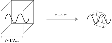
Figure 2: Schematic representation of Witten’s argument that a general coordinate transformation spoils the box used to define the modes that are integrated out in order to identify the emergent low-energy physics for energy scales well below $\Lambda_{\hbox{\tiny\it UV}}$.

In 1983, Laughlin explained the observed fractional quantum Hall effect in two-dimensional electronic systems by showing how such a system could form an incompressible quantum fluid whose excitations have charge $e/3$ ([laughlin]). That is, the low-energy theory of the interacting electrons in two spatial dimensions has composite degrees of freedom whose charge is a fraction of that of the electrons themselves. In 2001, Zhang and Hu used techniques similar to Laughlin’s to study the composite excitations of a higher-dimensional system ([zhang&hu]). They imagined a four-dimensional sphere in space, filled with fermions that interact via an $SU(2)$ gauge field. In the limit where the dimensionality of the representation of $SU(2)$ is taken to be very large, such a theory exhibits composite massless excitations of integer spin 1, 2 and higher.

Like other theories from solid state physics, Zhang and Hu’s proposal falls outside the scope of the Weinberg-Witten theorem because the proposed theory is not Lorentz-invariant: The vacuum of the theory is not empty and has a preferred rest-frame (the rest frame of the fermions). However, the authors argued that in the three-dimensional boundary of the four-dimensional sphere, a relativistic dispersion relation would hold. One might then imagine that the relativistic, three-dimensional world we inhabit might be the edge of a four-dimensional sphere filled with fermions. Photons and gravitons would be composite low-energy degrees of freedom, and the problems currently associated with gravity in the UV would be avoided. The authors also argue that massless bosons with spin 3 and higher might naturally decouple from other matter, thus explaining why they are not observed in nature.

In Chapter 2 we will discuss another proposal, dating back to the work of Dirac ([diracLV]) and Bjorken ([bjorken1]) for obtaining massless mediators as the Goldstone bosons of the spontaneous breaking of Lorentz violation. Such an arrangement evades the Weinberg-Witten theorem because the Lorentz invariance of the theory is realized non-linearly in the Goldstone bosons. Therefore the matrix elements in Eq. (69) will not be Lorentz-covariant.

Chapter 2 Goldstone photons and gravitons

In this chapter we will address some issues connected with the construction of models in which massless mediators are obtained as Goldstone bosons of the spontaneous breaking of Lorentz invariance (LI). This presentation is based largely on previously published work [LV1, CPT04].

1 Emergent mediators

In 1963, Bjorken proposed a mechanism for what he called the “dynamical generation of quantum electrodynamics” (QED) ([bjorken1]). His idea was to formulate a theory that would reproduce the phenomenology of standard QED, without invoking local $U(1)$ gauge invariance as an axiom. Instead, Bjorken proposed working with a self-interacting fermion field theory of the form

$${\cal L}=\bar{\psi}(i\partial\!\!\!/-m)\psi-\lambda(\bar{\psi}\gamma^{\mu}\psi)^{2}.$$ (1)

Bjorken then argued that in a theory such as that described by Eq. (1), composite “photons” could emerge as Goldstone bosons resulting from the presence of a condensate that spontaneously broke LI.

Conceptually, a useful way of understanding Bjorken’s proposal is to think of it as as a resurrection of the “lumineferous æther” ([Nambu1, Nambu2]): “empty” space is no longer really empty. Instead, the theory has a non-vanishing vacuum expectation value (VEV) for the current $j^{\mu}=\bar{\psi}\gamma^{\mu}\psi$. This VEV, in turn, leads to a massive background gauge field $A^{\mu}\propto j^{\mu}$, as in the well-known London equations for the theory of superconductors ([London]). Such a background spontaneously breaks Lorentz invariance and produces three massless excitations of $A^{\mu}$ (the Goldstone bosons) proportional to the changes $\delta j^{\mu}$ associated with the three broken Lorentz transformations.

Two of these Goldstone bosons can be interpreted as the usual transverse photons. The meaning of the third photon remains problematic. Bjorken originally interpreted it as the longitudinal photon in the temporal-gauge QED, which becomes identified with the Coulomb force (see also [Nambu1]). More recently, Kraus and Tomboulis have argued that the extra photon has an exotic dispersion relation and that its coupling to matter should be suppressed ([KrausTomboulis]).

Bjorken’s idea might not seem attractive today, since a theory such as Eq. (1) is not renormalizable, while the work of ’t Hooft and others has demonstrated that a locally gauge-invariant theory can always be renormalized ([thooft]). Furthermore, as detailed in Section 4, the gauge theories have had other very significant successes. Unless we take seriously the line of thought pursued in Chapter 1 that local gauge invariance is suspect because it is a redundancy of the mathematical description rather than a genuine physical symmetry, there would not appear to be, at this stage in our understanding of fundamental physics, any compelling reason to abandon local gauge invariance as an axiom for writing down interacting QFT’s. Furthermore, the arguments for the existence of a LI-breaking condensate in theories such as Eq. (1) have never been solid.

In 2002 Kraus and Tomboulis resurrected Bjorken’s idea for a different purpose of greater interest to contemporary theoretical physics: making a composite graviton ([KrausTomboulis]). They proposed what Bjorken might call “dynamical generation of gravity.” In this scenario a composite graviton would emerge as a Goldstone boson from the spontaneous breaking of Lorentz invariance in a theory of self-interacting fermions. Being a Goldstone boson, such a graviton would be forbidden from developing a potential, thus providing a solution to the “large cosmological constant problem:” the $\Lambda h^{\mu}_{~{}\mu}$ tadpole term for the graviton would vanish without fine-tuning (see Section LABEL:sect:cosmointro). This scheme would also seem to offer an unorthodox avenue to a renormalizable quantum theory of gravity, because the fermion self-interactions could be interpreted as coming from the integrating out, at low energies, of gauge bosons that have acquired large masses via the Higgs mechanism, so that Einstein gravity would be the low energy behavior of a renormalizable theory. This proposal would, of course, radically alter the nature of gravitational physics at very high energies. Related ideas had been previously considered in, for instance, [ohanian].

In [KrausTomboulis], the authors consider fermions coupled to gauge bosons that have acquired masses beyond the energy scale of interest. Then an effective low-energy theory can be obtained by integrating out those gauge bosons. We expect to obtain an effective Lagrangian of the form

$${\cal L} = \bar{\psi}(i\partial\!\!\!/-m)\psi+\sum_{n=1}^{\infty}\lambda_{n}(\bar{\psi}\gamma^{\mu}\psi)^{2n}$$ (2)

$$+\sum_{n=1}^{\infty}\mu_{n}\left[\bar{\psi}\frac{i}{2}(\gamma_{\mu}\buildrel\rightarrow\over{\partial}_{\nu}-\gamma_{\mu}\buildrel\leftarrow\over{\partial}_{\nu})\psi\right]^{2n}+\,\ldots~{},$$

where we have explicitly written out only two of the power series in fermion bilinears that we would in general expect to get from integrating out the gauge bosons.

One may then introduce an auxiliary field for each of these fermion bilinears. In this example we shall assign the label $A^{\mu}$ to the auxiliary field corresponding to $\bar{\psi}\gamma^{\mu}\psi$, and the label $h^{\mu\nu}$ to the field corresponding to $\bar{\psi}\frac{i}{2}(\gamma_{\mu}\buildrel\rightarrow\over{\partial}_{\nu}-\gamma_{\mu}\buildrel\leftarrow\over{\partial}_{\nu})\psi$. It is possible to write a Lagrangian that involves the auxiliary fields but not their derivatives, so that the corresponding algebraic equations of motion relating each auxiliary field to its corresponding fermion bilinear make that Lagrangian classically equivalent to Eq. (2). In this case the new Lagrangian would be of the form

$${\cal L}^{\prime} = (\eta^{\mu\nu}+h^{\mu\nu})\bar{\psi}\frac{i}{2}(\gamma_{\mu}\buildrel\rightarrow\over{\partial}_{\nu}-\gamma_{\mu}\buildrel\leftarrow\over{\partial}_{\nu})\psi-\bar{\psi}(A\!\!\!/+m)\psi+\ldots$$ (3)

$$-V_{A}(A^{2})-V_{h}(h^{2})+\ldots~{},$$

where $A^{2}\equiv A_{\mu}A^{\mu}$ and $h^{2}\equiv h_{\mu\nu}h^{\mu\nu}$. The ellipses in Eq. (3) correspond to terms with other auxiliary fields associated with more complicated fermion bilinears that were also omitted in Eq. (2).

We may then imagine that instead of having a single fermion species we have one very heavy fermion, $\psi_{1}$, and one lighter one, $\psi_{2}$. Since Eq. (3) has terms that couple both fermion species to the auxiliary fields, integrating out $\psi_{1}$ will then produce kinetic terms for $A^{\mu}$ and $h^{\mu\nu}$.

In the case of $A^{\mu}$ we can readily see that since it is minimally coupled to $\psi_{1}$, the kinetic terms obtained from integrating out the latter must be gauge-invariant (provided a gauge-invariant regulator is used). To lowest order in derivatives of $A^{\mu}$, we must then get the standard photon Lagrangian $-F_{\mu\nu}^{2}/4$. Since $A^{\mu}$ was also minimally coupled to $\psi_{2}$, we then have, at low energies, something that has begun to look like QED.

If $A^{\mu}$ has a non-zero VEV, LI is spontaneously broken, producing three massless Goldstone bosons, two of which may be interpreted as photons (see [KrausTomboulis] for a discussion of how the exotic physics of the other extraneous “photon” can be suppressed). The integrating out of $\psi_{1}$ and the assumption that $h^{\mu\nu}$ has a VEV, by similar arguments, yield a low-energy approximation to linearized gravity.

Fermion bilinears other than those we have written out explicitly in Eq. (2) have their own auxiliary fields with their own potentials. If those potentials do not themselves produce VEV’s for the auxiliary fields, then there would be no further Goldstone bosons, and one would expect, on general grounds, that those extra auxiliary fields would acquire masses of the order of the energy-momentum cutoff scale for our effective field theory, making them irrelevant at low energies.

The breaking of LI would be crucial for this kind of mechanism, not only because we know experimentally that photons and gravitons are massless or very nearly massless, but also because it allows us to evade the Weinberg-Witten theorem ([weinbergwitten]), as we discussed in Section 7.

Let us concentrate on the simpler case of the auxiliary field $A^{\mu}$. For the theory described by Eq. (3), the equation of motion for $A^{\mu}$ is

$$\frac{\partial{\cal L}^{\prime}}{\partial A_{\mu}}=-\bar{\psi}\gamma^{\mu}\psi-V^{\prime}(A^{2})\cdot 2A^{\mu}=0.$$ (4)

Solving for $\bar{\psi}\gamma^{\mu}\psi$ in Eq. (4) and substituting into both Eq. (2) and Eq. (3) we see that the condition for the Lagrangians ${\cal L}$ and ${\cal L}^{\prime}$ to be classically equivalent is a differential equation for $V(A^{2})$ in terms of the coefficients $\lambda_{n}$:

$$V(A^{2})=2A^{2}[V^{\prime}(A^{2})]-\sum_{n=1}^{\infty}\lambda_{n}2^{2n}A^{2n}[V^{\prime}(A^{2})]^{2n}.$$ (5)

It is suggested in [KrausTomboulis] that for some values of $\lambda_{n}$ the resulting potential $V(A^{2})$ might have a minimum away from $A^{2}=0$, and that this would give the LI-breaking VEV needed. It seems to us, however, that a minimum of $V(A^{2})$ away from the origin is not the correct thing to look for in order to obtain LI breaking. The Lagrangian in Eq. (3) contains $A^{\mu}$’s not just in the potential but also in the “interaction” term $A_{\mu}\bar{\psi}\gamma^{\mu}\psi$, which is not in any sense a small perturbation as it might be, say, in QED. In other words, the classical quantity $V(A^{2})$ is not a useful approximation to the quantum effective potential for the auxiliary field.

In fact, regardless of the values of the $\lambda_{n}$, Eq. (5) implies that $V(A^{2}=0)=0$, and also that at any point where $V^{\prime}(A^{2})=0$ the potential must be zero. Therefore, the existence of a classical extremum at $A^{2}=C\neq 0$ would imply that $V(C)=V(0)$, and unless the potential is discontinuous somewhere, this would require that $V^{\prime}$ (and therefore also $V$) vanish somewhere between $0$ and $C$, and so on ad infinitum. Thus the potential $V$ cannot have a classical minimum away from $A^{2}=0$, unless the potential has poles or some other discontinuity.

A similar observation applies to any fermion bilinear for which we might attempt this kind of procedure and therefore the issue arises as well when dealing with the proposal in [KrausTomboulis] for generating the graviton. It is not possible to sidestep this difficulty by including other auxiliary fields or other fermion bilinears, or even by imagining that we could start, instead of from Eq. (2), from a theory with interactions given by an arbitrary, possibly non-analytic function of the fermion bilinear $F(\mbox{bilinear})$. The problem can be traced to the fact that the equation of motion of any auxiliary field of this kind will always be of the form

$$0=-(\mbox{bilinear})-V^{\prime}(\mbox{field}^{2})\cdot 2\,\mbox{field}.$$ (6)

The point is that the vanishing of the first derivative of the potential or the vanishing of the auxiliary field itself will always, classically, imply that the fermion bilinear is zero. Classically at least, it would seem that the extrema of the potential would correspond to the same physical state as the zeroes of the auxiliary field.

2 Nambu and Jona-Lasinio model (review)

The complications we have discussed that emerge when one tries to implement LI breaking as proposed in [KrausTomboulis] do not, in retrospect, seem entirely surprising. A VEV for the auxiliary field would classically imply a VEV for the corresponding fermion bilinear, and therefore a trick such as rewriting a theory in a form like Eq. (3) should not, perhaps, be expected to uncover a physically significant phenomenon such as the spontaneous breaking of LI for a theory where it was not otherwise apparent that the fermion bilinear in question had a VEV. Let us therefore turn our attention to considering what would be required so that one might reasonably expect a fermion field theory to exhibit the kind of condensation that would give a VEV to a certain fermion bilinear.

If we allowed ourselves to be guided by purely classical intuition, it would seem likely that a VEV for a bilinear with derivatives (such as $\bar{\psi}\frac{i}{2}(\gamma_{\mu}\buildrel\rightarrow\over{\partial}_{\nu}-\gamma_{\mu}\buildrel\leftarrow\over{\partial}_{\nu})\psi$) might require nonstandard kinetic terms in the action. Whether or not this intuition is correct, we abandon consideration of such bilinears here as too complicated.

The simplest fermion bilinear is, of course, $\bar{\psi}\psi$. Being a Lorentz scalar, $\langle\bar{\psi}\psi\rangle\neq 0$ will not break LI. This kind of VEV was treated back in 1961 by Nambu and Jona-Lasinio, who used it to spontaneously break chiral symmetry in one of the early efforts to develop a theory of the strong nuclear interactions, before the advent of quantum chromodynamics (QCD) ([NJL]). It might be useful to review the original work of Nambu and Jona-Lasinio, as it may shed some light on the study of the possibility of giving VEV’s to other fermion bilinears that are not Lorentz scalars.

In their original paper, Nambu and Jona-Lasinio start from a self-interacting massless fermion field theory and propose that the strong interactions be mediated by pions, which appear as Goldstone bosons produced by the spontaneous breaking of the chiral symmetry associated with the transformation $\psi\mapsto\exp{(i\alpha\gamma^{5})}\psi$. This symmetry breaking is produced by a VEV for the fermion bilinear $\bar{\psi}\psi$. In other words, Nambu and Jona-Lasinio originally proposed what, by close analogy to Bjorken’s idea, would be the “dynamical generation of the strong interactions.”

Nambu and Jona-Lasinio start from a non-renormalizable quantum field theory with a four-fermion interaction that respects chiral symmetry:

$${\cal L}=i\bar{\psi}\partial\!\!\!/\psi-\frac{g}{2}[(\bar{\psi}\gamma^{\mu}\psi)^{2}-(\bar{\psi}\gamma^{\mu}\gamma^{5}\psi)^{2}].$$ (7)

Figure 1: Diagrammatic Schwinger-Dyson equation. The double line represents the primed propagator, which incorporates the self-energy term. The single line represents the unprimed propagator. 1PI${}^{\prime}$ stands for the sum of one-particle irreducible graphs with the primed propagator.

In order to argue for the presence of a chiral symmetry-breaking condensate in the theory described by Eq. (7), Nambu and Jona-Lasinio borrowed the technique of self-consistent field theory from solid state physics (see, for instance, [selfconsistent]). If one writes down a Lagrangian with a free and an interaction part, ${\cal L}={\cal L}_{0}+{\cal L}_{i}$, ordinarily one would then proceed to diagonalize ${\cal L}_{0}$ and treat ${\cal L}_{i}$ as a perturbation. In self-consistent field theory one instead rewrites the Lagrangian as ${\cal L}=({\cal L}_{0}+{\cal L}_{s})+({\cal L}_{i}-{\cal L}_{s})={\cal L}_{0}^{\prime}+{\cal L}_{i}^{\prime}$, where ${\cal L}_{s}$ is a self-interaction term, either bilinear or quadratic in the fields, such that ${\cal L}_{0}^{\prime}$ yields a linear equation of motion. Now ${\cal L}_{0}^{\prime}$ is diagonalized and ${\cal L}_{i}^{\prime}$ is treated as a perturbation.

In order to determine what the form of ${\cal L}_{s}$ is, one requires that the perturbation ${\cal L}_{i}^{\prime}$ not produce any additional self-energy effects. The name “self-consistent field theory” reflects the fact that in this technique ${\cal L}_{i}$ is found by computing a self-energy via a perturbative expansion in fields that already are subject to that self-energy, and then requiring that such a perturbative expansion not yield any additional self-energy effects.

Nambu and Jona-Lasinio proceed to make the ansatz that for Eq. (7) the self-interaction term will be of the form ${\cal L}_{s}=-m\bar{\psi}\psi$. Then, to first order in the coupling constant $g$, they proceed to compute the fermion self-energy $\Sigma^{\prime}(p)$, using the propagator $S^{\prime}(p)=i(p\!\!\!/-m)^{-1}$, which corresponds to the Lagrangian ${\cal L}_{0}^{\prime}=\bar{\psi}(i\partial\!\!\!/-m)\psi$ that incorporates the proposed self-energy term.

The next step is to apply the self-consistency condition using the Schwinger-Dyson equation for the propagator

$$S^{\prime}(x-y)=S(x-y)+\int d^{4}z\,S(x-z)\Sigma^{\prime}(0)S^{\prime}(z-y)~{},$$ (8)

which is represented diagrammatically in Fig. 1. The primes indicate quantities that correspond to a free Lagrangian ${\cal L}_{0}^{\prime}$ that incorporates the self-energy term, whereas the unprimed quantities correspond to the ordinary free Lagrangian ${\cal L}_{0}$. For $\Sigma^{\prime}$ we will use the approximation shown in Fig. 2, valid to first order in the coupling constant $g$.

After Fourier transforming Eq. (8) and summing the left side as a geometric series, we find that the self-consistency condition may be written, in our approximation, as

$$m=\Sigma^{\prime}(0)=\frac{gmi}{2\pi^{4}}\int\frac{d^{4}p}{p^{2}-m^{2}+i\epsilon}.$$ (9)

If we evaluate the momentum integral by Wick rotation and regularize its divergence by introducing a Lorentz-invariant energy-momentum cutoff $p^{2}<\Lambda^{2}$ we find

$$\frac{2\pi^{2}m}{g\Lambda^{2}}=m\left[1-\frac{m^{2}}{\Lambda^{2}}\log{\left(\frac{\Lambda^{2}}{m^{2}}+1\right)}\right].$$ (10)

Figure 2: Diagrammatic equation for the primed self-energy. We will work to first order in the fermion self-coupling constant $g$.

This equation will always have the trivial solution $m=0$, which corresponds to the vanishing of the proposed self-interaction term ${\cal L}_{i}$. But if

$$0<\frac{2\pi^{2}}{g\Lambda^{2}}<1$$ (11)

then there may also be a non-trivial solution to Eq. (10), i.e., a non-zero $m$ for which the condition of self-consistency is met. For a rigorous treatment of the relation between non-trivial solutions of this self-consistent equation and local extrema in the Wilsonian effective potential for the corresponding fermion bilinears, see [Aoki] and the references therein.

In this model (which from now on we shall refer to as NJL), we see that if the interaction between fermions and antifermions is attractive ($g>0$) and strong enough ($\frac{2\pi^{2}}{g\Lambda^{2}}<1$) it might be energetically favorable to form a fermion-antifermion condensate. This is reasonable to expect in this case because the particles have no bare mass and thus the energy cost of producing them is small. The resulting condensate would have zero net charge, as well as zero total momentum and spin. Therefore it must pair a left-handed fermion $\psi_{L}=\frac{1}{2}(1-\gamma^{5})\psi$ with the antiparticle of a right-handed fermion $\psi_{R}=\frac{1}{2}(1+\gamma^{5})\psi$, and vice versa. This is the mass-term self-interaction ${\cal L}_{i}=-m\bar{\psi}\psi=-m(\bar{\psi}_{L}\psi_{R}+\bar{\psi}_{R}\psi_{L})$ that NJL studies.

After QCD became the accepted theory of the strong interactions, the ideas behind the NJL mechanism remained useful. The $u$ and $d$ quarks are not massless (nor is $u$-$d$ flavor isospin an exact symmetry) but their bare masses are believed to be quite small compared to their effective masses in baryons and mesons, so that the formation of $\bar{u}u$ and $\bar{d}d$ condensates represents the spontaneous breaking of an approximate chiral symmetry. Interpreting the pions (which are fairly light) as the pseudo-Goldstone bosons generated by the spontaneous breaking of the approximate $SU(2)_{R}\times SU(2)_{L}$ chiral isospin symmetry down to just $SU(2)$, proved a fruitful line of thought from the point of view of the phenomenology of the strong interaction.

Condition Eq. (11) has a natural interpretation if we think of the interaction in Eq. (7) as mediated by massive gauge bosons with zero momentum and coupling $e$. For it to be reasonable to neglect boson momentum in the effective theory, the mass $\mu$ of the bosons should be $\mu>\Lambda$. If $e^{2}<2\pi^{2}$ then $g=e^{2}/\mu^{2}<2\pi^{2}/\Lambda^{2}$, which violates Eq. (11). Therefore for chiral symmetry breaking to happen, the coupling $e$ should be quite large, making the renormalizable theory nonperturbative. This is acceptable because the factor of $1/\mu^{2}$ allows the perturbative calculations we have carried out in the effective theory Eq. (7). This is why the NJL mechanism is modernly thought of as a model for a phenomenon of non-perturbative QCD.

3 An NJL-style argument for breaking LI

We have reviewed how NJL formulated a model that exhibited a non-zero VEV for the fermion bilinear $\bar{\psi}\psi$. The next simplest fermion bilinear that we might consider is $\bar{\psi}\gamma^{\mu}\psi$, which was the one that Bjorken, Kraus, and Tomboulis considered when they discussed the “dynamical generation of QED.” This particular fermion bilinear is especially interesting because it corresponds to the $U(1)$ conserved current, and also because it is the simplest bilinear with an odd number of Lorentz tensor indices, so that a non-zero VEV for it would break not only LI but also charge (C), charge-parity (CP), and charge-parity-time (CPT) reversal invariance. C and CP may not be symmetries of the Lagrangian, as indeed they are not in the standard model, but by a celebrated result CPT must be an invariance of any reasonable theory (see [CPT] and references therein). This invariance, however, may well be spontaneously broken, as it would be by any VEV with an odd number of Lorentz indices.

Before proceeding, however, it may be advisable to try to develop some physical intuition about what would be required for a fermion bilinear like $\bar{\psi}\gamma^{\mu}\psi$ to exhibit a VEV. If we choose a representation of the gamma matrix algebra and use it to write out $(\bar{\psi}\gamma^{\mu}\psi)^{2}$ for an arbitrary Dirac bispinor $\psi$, we may check that $(\bar{\psi}\gamma^{\mu}\psi)^{2}\geq 0$ for the choice of mostly negative metric $g^{\mu\nu}=\mbox{diag}(1,-1,-1,-1)$. That is, $\bar{\psi}\gamma^{\mu}\psi$ is time-like. This has an intuitive explanation, based on the observation that $\bar{\psi}\gamma^{\mu}\psi$ is a conserved fermion-number current density. Classically a charge density $\rho$ moving with a velocity $\bm{v}$ will produce a current $j^{\mu}=(\rho,\rho\bm{v})$ (in units of $c=1$). Therefore the relativistic requirement that the charge density not move faster than the speed of light in any frame of reference implies that $j^{2}\geq 0$. Considerations of causality make it natural to expect that something similar would be true of $\bar{\psi}\gamma^{\mu}\psi$.

For any time-like Lorentz vector $n^{\mu}$ it is possible to find a Lorentz transformation that maps it to a vector $n^{\prime\mu}$ with only one non-vanishing component: $n^{\prime 0}$. For a constant current density $j^{\mu}$, this means that for $j^{\mu}$ to be non-zero there must be a charge density $j^{0}$, which has a rest frame. Therefore we only expect to see a VEV for $\bar{\psi}\gamma^{\mu}\psi$ if our theory somehow has a vacuum with a non-zero fermion number density. The consequent spontaneous breaking of LI may be seen as the introduction of a preferred reference frame: the rest frame of the vacuum charge.

In the literature of finite density quantum field theory and of color superconductivity (see, for instance, [colorsuperconduct1] and [colorsuperconduct2]), the Lagrangians discussed are explicitly non-Lorentz-invariant because they contain chemical potential terms of the form $f\cdot\bar{\psi}\gamma^{0}\psi$ . This term appears in theories whose ground state has a non-zero fermion number because, by the Pauli exclusion principle, new fermions must be added just above the Fermi surface, i.e., at energies higher than those already occupied by the pre-existing fermions, while holes (which can be thought of as antifermions) should be made by removing fermions at that Fermi surface. The result is an energy shift that depends on the number of fermions already present and which has opposite signs for fermions and antifermions, as illustrated in Fig. 3.

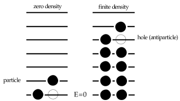
Figure 3: Fermion and antifermion energies in QFT, at zero density (left) and at finite density (right). Finite density introduces a chemical potential term $-f\cdot\bar{\psi}\gamma^{0}\psi$ into the fermion Lagrangian.

The physical picture that emerges is now, hopefully, clearer: A theory with a VEV for $\bar{\psi}\gamma^{\mu}\psi$ is one with a condensate that has non-zero fermion number. This means that only theories with some form of attractive interaction between particles with the same sign in fermion number may be expected to produce such a VEV. The situation is closely analogous to BCS superconductivity ([BCS]), in which a phonon-mediated attractive interaction between electrons allows the presence of a condensate with non-zero electric charge. Note that in the NJL model, the condensate was composed of fermion-antifermion pairs, and therefore clearly $\langle\bar{\psi}\gamma^{0}\psi\rangle=0$, which implies $\langle\bar{\psi}\gamma^{\mu}\psi\rangle=0$. It should now be clear why a VEV for $\bar{\psi}\gamma^{\mu}\psi$ would break not only LI but also C, CP, and CPT. This picture also helps to clarify the nature of the Goldstone bosons that we will be invoking as mediators of the electromagnetic interaction: They are density waves in the background “Dirac sea,” whose energy at infinite wavelengths vanishes because they are then proportional to the broken boosts.

There is an easy way to write a theory that will have a VEV for a $U(1)$ conserved current: to couple a massive photon to such a current via a purely imaginary charge. To see this, let us write a Proca Lagrangian for a massive photon field with an external source:

$${\cal L}=-\frac{1}{4}F_{\mu\nu}^{2}+\frac{\mu^{2}}{2}A^{2}-j_{\mu}A^{\mu}.$$ (12)

The equation of motion for the photon field is

$$\partial_{\mu}F^{\mu\nu}=j^{\nu}-\mu^{2}A^{\nu}.$$ (13)

At energy scales well below the photon mass $\mu$, the kinetic term $-F_{\mu\nu}^{2}/4$ may be neglected with respect to the mass term $\mu^{2}A^{2}/2$. We may then integrate out the photon at zero momentum by solving the equation of motion Eq. (13) for the photon field $A^{\mu}$ with its conjugate momenta $F^{\mu\nu}$ set to zero, and substituting the result back into the Lagrangian in Eq. (12). The resulting low-energy effective field theory has the Hamiltonian

$$\mathcal{H}_{\mathrm{effective}}=\frac{j^{2}}{2\mu^{2}}.$$ (14)

Nothing interesting happens if the source is a timelike current density, since in that case Eq. (14) has its minimum at $j^{\mu}=0$. But if we were to make the charge coupling to the photon imaginary (e.g., $j^{\mu}=ie\bar{\psi}\gamma^{\mu}\psi$ for $e$ real), then $j^{2}$ is actually always negative (recall that $(\bar{\psi}\gamma^{\mu}\psi)^{2}$ is always positive) and we get a “potential” with the wrong sign, so that the energy can be made arbitrarily low by decreasing $j^{2}$. If we make $j^{\mu}$ dynamical by adding to the Lagrangian terms corresponding to the field that sets up the current, we might expect, for certain parameters in the theory, that the energy be minimized for a finite value of $j^{\mu}$.

By making the charge purely imaginary, our effective theory at energy scales much lower than the photon mass $\mu$ will look similar to Eq. (7), except that the four-fermion interaction in the effective Lagrangian will be $e^{2}(\bar{\psi}\gamma^{\mu}\psi)^{2}/2\mu^{2}$ (with an overall positive, rather than a negative, sign). What this means is that fermions are attracting fermions and antifermions are attracting antifermions, rather than what we had in NJL (and in QED): attraction between a fermion and an antifermion. Condensation, if it occurs, will here produce a net fermion number, spontaneously breaking C, CP, and CPT.

Let us analyze this situation again more rigorously using self-consistent field theory methods, following Nambu and Jona-Lasinio. For this we consider a fermion field with the usual free Lagrangian ${\cal L}_{0}=\bar{\psi}(i\partial\!\!\!/-m_{0})\psi$ and pose as our self-consistent ansatz:

$${\cal L}_{s}=-(m-m_{0})\bar{\psi}\psi-f\bar{\psi}\gamma^{0}\psi.$$ (15)

The corresponding momentum-space propagator for ${\cal L}_{0}^{\prime}={\cal L}_{0}+{\cal L}_{s}$ is, therefore,

$$S^{\prime}(k)=i(k\!\!\!/-f\gamma^{0}-m)^{-1}.$$ (16)

Now let us suppose that the interaction term looks like

$${\cal L}_{i}=\frac{g}{2}(\bar{\psi}\gamma^{\mu}\psi)^{2}.$$ (17)

To obtain the Feynman rules corresponding to Eq. (17) we note that this is what we would obtain in massive QED if we replaced the charge $e$ by $ie$ and the usual photon propagator by $ig^{\mu\nu}/\mu^{2}$, with $g=e^{2}/\mu^{2}$. Therefore to compute the self-energy we will rely on the identity represented in Fig. LABEL:contractions. (In QED the second diagram on the right-hand side of Fig. LABEL:contractions would vanish by Furry’s theorem, but in our case the propagator in the loop will have a chemical potential term that breaks the C invariance on which Furry’s theorem depends.)

fmfcontractions

$$\text{<span id="Ch2.Ex4.m1.1.1.1nest" class="ltx\_inline-block ltx\_parbox ltx\_align\_middle" style="width:71.1pt;"> <span id="Ch2.Ex4.m1.1.1.1.2nest" class="ltx\_p">(25,20) i o plain,tension=2/3i,z,z,o z</span> </span>}=\text{<span id="Ch2.Ex4.m1.1.3.1nest" class="ltx\_inline-block ltx\_parbox ltx\_align\_middle" style="width:71.1pt;"> <span id="Ch2.Ex4.m1.1.3.1.2nest" class="ltx\_p">(25,20) i o plaini,z1 photon,tension=1/3z1,z2 plain,right,tension=0z2,z1 plainz2,o</span> </span>}+\text{<span id="Ch2.Ex4.m1.1.5.1nest" class="ltx\_inline-block ltx\_parbox ltx\_align\_middle" style="width:71.1pt;"> <span id="Ch2.Ex4.m1.1.5.1.2nest" class="ltx\_p">(25,20) i,o,z,zl i(0,.5h) o(w,.5h) z(.5w,.5h) zl(.5w,.8h) l=</span> <span id="Ch2.Ex3nest" class="ltx\_equation ltx\_eqn\_table"> <span><span class="ltx\_equation ltx\_eqn\_row ltx\_align\_baseline"> <span class="ltx\_eqn\_cell ltx\_eqn\_center\_padleft"></span> <span class="ltx\_eqn\_cell ltx\_align\_center"></span> <span class="ltx\_eqn\_cell ltx\_eqn\_center\_padright"></span></span></span> </span> <span id="Ch2.Ex4.m1.1.5.1.3nest" class="ltx\_p">zl plaini–z plainz–o photonz–zl plainfullcircle scaled .4h shifted (.5w,h)</span> </span>}$$ Figure 4

Figure 4: Th