Screening length in plasma winds

Abstract:

We study the screening length $L_{s}$ of a heavy quark-antiquark pair in strongly coupled gauge theory plasmas flowing at velocity $v$. Using the AdS/CFT correspondence we investigate, analytically, the screening length in the ultra-relativistic limit. We develop a procedure that allows us to find the scaling exponent for a large class of backgrounds. We find that for conformal theories the screening length is $(\mbox{boosted energy density})^{-1/d}$. As examples of conformal backgrounds we study R-charged black holes and Schwarzschild-anti-deSitter black holes in $(d+1)$-dimensions. For non-conformal theories, we find that the exponent deviates from $-1/d$. As examples we study the non-extremal Klebanov-Tseytlin and D$p$-brane geometries. We find an interesting relation between the deviation of the scaling exponent from the conformal value and the speed of sound.

1 Introduction

The analysis of the quark gluon plasma (QGP) produced in relativistic heavy ion collisions is, undoubtedly, a challenging task. One of the main difficulties is that in the temperature range of current and near-future experiments QCD is believed to be strongly coupled. Thus, one often focuses on the generic signatures of QGP. For example,

1. The elliptic flow

2. The jet quenching

3. $J/\Psi$-suppression.

The first signature, the elliptic flow, is interpreted as a consequence of the QGP having a very low viscosity [1, 2]. In [3], Policastro, Son and Starinets pioneered the use of the AdS/CFT correspondence to study a strongly coupled plasma. It was found that the AdS/CFT prediction of the shear viscosity is in very good agreement with the value derived from the elliptic flow [4]-[11]. (See Ref. [12] for a review.) This success indicates that AdS/CFT might be a good tool to gain some insight in the physics of QGP. It is thus natural to ask what are the AdS/CFT descriptions of the other QGP signatures and what can we learn from them. In fact, AdS/CFT descriptions of jet quenching and energy loss have been proposed recently [13]-[16]. (See Refs. [17]-[24] for extensions to other backgrounds and Ref. [21] for comparison of these different proposals. See also Ref. [25] for an early attempt.)

The next natural step is to investigate $J/\Psi$-suppression. Since $J/\Psi$ is heavy, charm pair production occurs only at the early stages of the nuclear collision. However, if the production occurs in the plasma medium, charmonium formation is suppressed due to Debye screening. One technical difficulty is that the $c\bar{c}$ pair is not produced at rest relative to the plasma. Therefore, it is expected that the screening length will be velocity dependent. A dynamical calculation of the screening potential has been done only for the Abelian plasma [28].

Recently, there has been an interesting proposal by Liu, Rajagopal and Wiedemann to model charmonium suppression via the AdS/CFT correspondence [26]. The authors considered a boosted black hole and computed the screening length in the quark-antiquark rest frame. In Ref. [27], the authors studied the equivalent problem of a quark-antiquark pair moving in a thermal background and calculated the screening length as well. The main lessons drawn from Ref. [26] are,

1. The screening length is proportional to $(\mbox{boosted energy density})^{-1/4}$.

2. Aside from the boost factor, $(1-v^{2})^{1/4}$,  the screening length has only a mild dependence on the wind velocity $v$.

3. The length is minimum when $\theta=\pi/2$ and maximum when $\theta=0$, where $\theta$ is the angle of the quark-antiquark pair (dipole) relative to the plasma wind.

The main focus in Ref. [26] is the five-dimensional Schwarzschild-AdS black hole (${\rm SAdS}_{5}$), which is dual to the ${\cal N}=4$ super-Yang-Mills theory (SYM) at finite temperature. Even in that simple background, numerical computations were needed in order to see the full details of the screening length.

In this paper, we focus on the ultra-relativistic limit, where analytic computations are possible. This makes it easier to carry out the analysis in various, more involved, backgrounds. We study the scaling of the screening length with the energy density and the velocity. Our results are summarized as follows:

1. For conformal theories, we find the behavior

   $$(\mbox{screening length})\propto(\mbox{boosted energy density})^{-1/d}~{},$$ (1.1)

   where $d$ denotes the number of dimensions of a dual gauge theory. Examples are ${\rm SAdS}_{d+1}\>$and R-charged black holes with three generic charges.

2. In particular, in the ultra-relativistic limit, the screening length at finite chemical potential is the same as the one at zero chemical potential for a given energy density.

3. For non-conformal theories, the exponent deviates from $1/d$. Examples are the non-extremal Klebanov-Tseytlin (KT) geometry and the D$p$-brane solution. For small nonconformality, the deviation is proportional to the parameter of the nonconformality. We conjecture a universal expression of the deviation written in terms of the speed of sound.

These results are in a sense natural; conformal theories have only few dimensionful parameters so the screening length should behave as Eq. (1.1) from dimensional grounds. On the other hand, non-conformal theories have other dimensionful parameters, so the screening length is not determined from dimensional analysis. However, even for conformal theories, the details are not determined from dimensional analysis alone. For example, in the ultra-relativistic limit, the screening length in a R-charged black hole background is independent of the chemical potential. Also, for non-conformal theories, the exponent turns out to be smaller than the one for the conformal examples.

In the next section, we will derive the relevant equations of motion for general backgrounds. We then proceed to analyze conformal theories in Sec. 4, where we also develop a general procedure to treat a large class of backgrounds. As examples, we calculate the screening length for R-charged black holes and ${\rm SAdS}_{d+1}$. In Sec. 5, we analyze two non-conformal theories: the non-extremal Klebanov-Tseytlin solution and D$p$-branes backgrounds. We conclude in Sec. 6 with discussion, implications and future directions.

2 General setup

In the AdS/CFT framework, a heavy quark may be realized by a fundamental string which stretches from the asymptotic infinity (or from a “flavor brane”) to the black hole horizon. This string transforms as a fundamental representation; In this sense, the string represents a “quark.” The fundamental string has an extension and the tension, so the string has a large mass, which means that the string represents a heavy quark.

For a $q\bar{q}$ pair, two individual strings extending to the boundary is not the lowest energy configuration. Instead, it is energetically favorable to have a single string that connects the pair. The energy difference is interpreted as a $q\bar{q}$ potential and has been widely studied in the past from the AdS/CFT perspective. At finite temperature [29, 30], it is no longer true that a string connecting the $q\bar{q}$ pair is always the lowest energy configuration; for large enough separation of the pair, isolated strings are favorable energetically. This phenomenon is the dual description of Debye screening in AdS/CFT. In Ref. [26], the authors computed $q\bar{q}$ screening length in the $q\bar{q}$ rest frame, i.e., they considered the plasma flowing at a velocity $v$. Such a “plasma wind” is obtained by boosting a black hole background.

2.1 Equations of motion

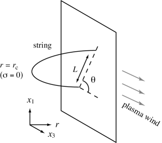
Figure 1: The fundamental string connecting the quark-antiquark pair. (The shape of the string should not be taken seriously.)

In order to consider the screening length in the dipole rest frame, we boost the background metric. We assume an unboosted metric of the form

$$ds^{2}=g_{xx}\,\{-(1-h)dt^{2}+dx_{i}^{2}\}+g_{rr}\,dr^{2}+\cdots~{}.$$ (2.1)

Consider the plasma wind in the $x_{3}$-direction, so the boosted metric is

$$-(1-h)dt^{2}+dx_{3}^{2}$$ (2.2)

$$\rightarrow-(1-h\cosh^{2}{\eta})dt^{2}-2h\sinh\eta\cosh\eta\,dtdx_{3}+(1+h\sinh^{2}{\eta})dx_{3}^{2}~{},$$

where $v$ is the wind velocity, $\cosh\eta=\gamma$,   $\sinh\eta=\gamma v$, and $\gamma=1/\sqrt{1-v^{2}}$.

The dynamics of the fundamental string is governed by the Nambu-Goto action. The quark-antiquark pair is chosen to lie in the $(x_{1},x_{3})$-plane at an angle $\theta$ relative to the wind (See Fig. 1). Thus, we choose the gauge $\tau=t,~{}\sigma=x_{1}$ and consider the configuration

$$x_{3}=x_{3}(\sigma)~{},\quad r=r(\sigma)~{},\quad\mbox{constant otherwise}.$$ (2.3)

Then, the Nambu-Goto action (in the string metric ) becomes

$$S=\frac{-1}{2\pi l_{s}^{2}}\int d\sigma^{2}~{}{\cal L} = \frac{-1}{2\pi l_{s}^{2}}\int d\sigma^{2}~{}\sqrt{-\mbox{det}\,G_{ab}}$$ (2.4)

$$= \frac{-1}{2\pi l_{s}^{2}}\int d\sigma^{2}~{}\sqrt{|G_{00}|(G_{11}+G_{33}x_{3}^{\prime 2}+G_{rr}r^{\prime 2})+G_{03}^{2}x_{3}^{\prime 2}}~{}.$$ (2.5)

Here, we used the boosted metric components such as $G_{03}$ and $~{}{}^{\prime}=d/d\sigma$. The conserved quantities are

$$-q := \left(\frac{\partial{\cal L}}{\partial r^{\prime}}\right)r^{\prime}+\left(\frac{\partial{\cal L}}{\partial x_{3}^{\prime}}\right)x_{3}^{\prime}-{\cal L}~{},$$ (2.6)

$$p := \frac{\partial{\cal L}}{\partial x_{3}^{\prime}}~{},$$ (2.7)

which become

$$q^{2}r^{\prime 2} = \frac{g_{xx}}{g_{rr}}\left[\frac{1-h\cosh^{2}{\eta}}{1-h}\left\{g_{xx}^{2}(1-h)-p^{2}\right\}-q^{2}\right]=:{\cal F}(r)~{},$$ (2.8)

$$q~{}x_{3}^{\prime} = p\,\frac{1-h\cosh^{2}{\eta}}{1-h}~{},$$ (2.9)

or equivalently,

$$x_{1} = \sigma=q\int\frac{dr}{\sqrt{{\cal F}}}~{},$$ (2.10)

$$x_{3} = \int dr\frac{dx_{3}}{dr}=p\int\frac{dr}{\sqrt{{\cal F}}}\frac{1-h\cosh^{2}{\eta}}{1-h}$$ (2.11)

$$= p\left[\frac{x_{1}}{q}-\sinh^{2}{\eta}\int\frac{dr}{\sqrt{{\cal F}}}\frac{h}{1-h}\right]~{}.$$

The string stretches from asymptotic infinity and reaches a turning point $r=r_{c}$ defined by ${\cal F}(r_{c})=0$. Then, the string goes back to asymptotic infinity. From the symmetry, the turning point occurs at $\sigma=0$. Then the boundary conditions are summarized as,

$$\begin{array}[]{ll}r(\sigma=0)=r_{c}~{},&{\cal F}(r_{c})=0~{},\\ r(\sigma=L\sin\theta/2)=\infty~{},&x_{3}(\sigma=L\sin\theta/2)=\frac{L}{2}\,\cos\theta~{}.\end{array}$$ (2.14)

where $L$ is the dipole length. The boundary conditions determine the integration constants $p$ and $q$ in terms of $L$ and $\theta$:

$$\frac{L}{2}\,\sin\theta = q\,I_{s}(p,q,\eta)~{},$$ (2.15)

$$\frac{L}{2}\,\cos\theta = p\,\Big{[}~{}I_{s}(p,q,\eta)-\sinh^{2}\eta\,I_{c}(p,q,\eta)~{}\Big{]}~{},$$ (2.16)

where

$$I_{s}(p,q,\eta) := \int^{\infty}_{r_{c}}\frac{dr}{\sqrt{{\cal F}}}~{},$$ (2.17)

$$I_{c}(p,q,\eta) := \int^{\infty}_{r_{c}}\frac{dr}{\sqrt{{\cal F}}}\,\frac{h}{1-h}~{}.$$ (2.18)

The energy is given by

$$E = -\frac{S}{T}$$ (2.19)

$$= \frac{1}{\pi l_{s}^{2}}\int_{r_{c}}^{\infty}dr\,\sqrt{g_{xx}g_{rr}(1-h\cosh^{2}{\eta})}\sqrt{\frac{g_{xx}}{g_{rr}{\cal F}}(q^{2}+p^{2}\frac{1-h\cosh^{2}{\eta}}{1-h})+1}~{}.$$

As usual, this energy can be made finite by subtracting the self-energy of a disconnected quark and antiquark pair which is

$$E_{0}=\frac{1}{\pi l_{s}^{2}}\int_{r_{0}}^{\infty}dr\,\sqrt{g_{xx}g_{rr}(1-h\cosh^{2}{\eta})}~{},$$ (2.20)

where $r_{0}$ is the location of the horizon.

Two special cases are worth discussing separately.

1. $\theta=\pi/2$: This is the case when the plasma wind is perpendicular to the dipole. In this case, Eq. (2.16) implies $p=0$. The integration constant $q$ can be determined from

   $$L=2q\int_{r_{c}}^{\infty}\frac{\sqrt{g_{rr}}~{}dr}{\sqrt{g_{xx}\{(1-h\cosh^{2}{\eta})g_{xx}^{2}-q^{2}\}}}~{}.$$ (2.21)

2. $\theta=0$: This is the case when the plasma wind is parallel to the dipole. In this case, Eq. (2.15) implies $q=0$. Then,

   $$L=2p\int_{r_{c}}^{\infty}dr\frac{1}{\sqrt{{\cal F}|_{q=0}}}\frac{1-h\cosh^{2}{\eta}}{1-h}~{}.$$ (2.22)

2.2 AdS/CFT dictionary

Some well-known AdS/CFT dictionary is summarized here. This dictionary is valid for ${\rm AdS}_{5}$, R-charged black holes, and the D$p$-brane. Roughly speaking, on the left-hand side we have gravity quantities which are written in terms of gauge theory quantities on the right-hand side.

$$16\pi G_{10} = (2\pi)^{7}g_{s}^{2}l_{s}^{8}~{},$$ (2.23)

$$R^{7-p} = \frac{(2\pi)^{7-p}}{(7-p)\Omega_{8-p}}g_{s}N_{c}l_{s}^{7-p}\qquad\mbox{($R$ in terms of $N_{c}$)},$$ (2.24)

$$2(2\pi)^{p-2}\,g_{s}\,l_{s}^{p-3} = g_{\rm YM}^{2}\qquad\mbox{($g_{s}$ in terms of $g_{\rm YM}$)},$$ (2.25)

where

$$\begin{array}[]{rl}G_{10}:&\mbox{10-dimensional Newton constant}\\ g_{s}:&\mbox{string coupling}\\ R:&\mbox{AdS radius}\\ N_{c}:&\mbox{number of colors}\\ g_{\rm YM}:&\mbox{YM coupling}\\ \Omega:&S^{n}\mbox{ volume of unit radius; }\Omega_{n}=2\pi^{\frac{n+1}{2}}/\Gamma(\frac{n+1}{2})~{}.\end{array}$$ (2.32)

When $p=3$,

$$16\pi G_{10} = (2\pi)^{7}\frac{R^{8}}{(4\pi N_{c})^{2}}~{},$$ (2.33)

$$(R/l_{s})^{4} = \lambda~{},$$ (2.34)

where $\lambda$ is the ’t Hooft coupling. Below we often consider effective five-dimensional theories with the five-dimensional Newton constant given by

$$G_{5}=\frac{G_{10}}{R^{5}\Omega_{5}}=\frac{\pi R^{3}}{2N_{c}^{2}}~{}.$$ (2.35)

3 Leading behavior of the screening length

3.1 An example: ${\rm SAdS}_{5}\>$

As an example, let us start with the ${\rm SAdS}_{5}\>$case. This has been studied previously in Refs. [26, 27]. Here we study it analytically in the ultra-relativistic limit. The ${\rm SAdS}_{5}\>$black hole is given by

$$ds^{2}=-\left(\frac{r}{R}\right)^{2}\left\{1-\left(\frac{r_{0}}{r}\right)^{4}\right\}dt^{2}+\frac{dr^{2}}{\left(\frac{r}{R}\right)^{2}\{1-(\frac{r_{0}}{r})^{4}\}}+\left(\frac{r}{R}\right)^{2}(dx_{1}^{2}+dx_{2}^{2}+dx_{3}^{2})~{}.$$ (3.1)

The temperature $T$ and the (unboosted) energy density $\epsilon_{0}$ of the black hole are given by

$$T = \frac{r_{0}}{\pi R^{2}},$$ (3.2)

$$\epsilon_{0} = \frac{3}{16\pi G_{5}}\frac{r_{0}^{4}}{R^{5}}=\frac{3}{8}\pi^{2}N_{c}^{2}T^{4}.$$ (3.3)

For $\theta=\pi/2$, Eq. (2.21) becomes

$$L_{\rm SAdS}(\theta=\pi/2)=2\mathfrak{q}\,\frac{R^{2}}{r_{0}}\int_{y_{c}}^{\infty}dy\frac{1}{\sqrt{(y^{4}-1)(y^{4}-y_{c}^{4})}}~{},$$ (3.4)

where we used the dimensionless variables

$$y:=\frac{r}{r_{0}}~{},\quad\mathfrak{q}:=\left(\frac{R}{r_{0}}\right)^{2}q~{},\quad\mathfrak{p}:=\left(\frac{R}{r_{0}}\right)^{2}p~{},$$ (3.5)

and $y_{c}$ is the turning point given by $y_{c}^{4}:=\cosh^{2}{\eta}+\mathfrak{q}^{2}$.

The above integral Eq. (3.4) can be evaluated numerically but is slightly involved since one in interested in $L_{\rm SAdS}$ as a function of $\mathfrak{q}$. We choose not to follow the numerical route; Instead, we investigate analytically the ultra-relativistic limit of Eq. (3.4). For large $\eta$, $y_{c}\gg 1$, so the integral reduces to

$$L_{\rm SAdS}(\theta=\pi/2) \xrightarrow{\eta\gg 1} 2\mathfrak{q}\,\frac{R^{2}}{r_{0}}\int_{y_{c}}^{\infty}dy\frac{1}{y^{2}\sqrt{y^{4}-y_{c}^{4}}}$$ (3.6)

$$= 2\sqrt{\pi}\frac{\Gamma(3/4)}{\Gamma(1/4)}\frac{\mathfrak{q}}{(\cosh^{2}{\eta}+\mathfrak{q}^{2})^{\frac{3}{4}}}\frac{R^{2}}{r_{0}}~{}.$$ (3.7)

We are interested in the behavior of $L_{\rm SAdS}$ as a function of $\mathfrak{q}$. The length $L_{\rm SAdS}$ goes to zero both for small $\mathfrak{q}$ and for large $\mathfrak{q}$. Thus, there is a maximum value $L_{s}$ at some $\mathfrak{q}_{m}$. This means that there is no extremal world-sheet which binds the quark-antiquark pair for $L>L_{s}$, so this $L_{s}$ is defined as a screening length in Ref. [26]. The maximum of $L_{\rm SAdS}$ is given by

$$L_{s}^{\rm SAdS}(\theta=\pi/2) = \frac{2\sqrt{2\pi}}{3^{3/4}}\frac{\Gamma(3/4)}{\Gamma(1/4)}\frac{1}{\sqrt{\cosh\eta}}\frac{R^{2}}{r_{0}}\qquad\mbox{at $\mathfrak{q}_{m}=\sqrt{2}\cosh\eta$}$$ (3.8)

$$\sim \frac{0.743}{\sqrt{\cosh\eta}}\frac{R^{2}}{r_{0}}~{}.$$ (3.9)

Rewriting in terms of gauge theory variables, the screening length $L_{s}$ is given by

$$L_{s}^{\rm SAdS}(\theta=\pi/2)\sim\frac{0.743}{\sqrt{\cosh\eta}}\frac{1}{\pi T}~{}.$$ (3.10)

This parametrization in terms of temperature was adopted in [26, 27]. One can equally express the result in terms of energy density:

$$L_{s}^{\rm SAdS}(\theta=\pi/2) = \frac{2^{3/4}}{\sqrt{3}}\frac{\Gamma(3/4)}{\Gamma(1/4)}\frac{\sqrt{N_{c}}}{(\epsilon_{0}\cosh^{2}{\eta})^{1/4}}$$ (3.11)

$$\sim 0.328\frac{\sqrt{N_{c}}}{(\epsilon_{0}\cosh^{2}{\eta})^{1/4}}~{}.$$ (3.12)

The choice of these parametrizations does not matter for ${\rm SAdS}_{5}\>$since there is no other dimensionful quantities. But it does matter when one has other dimensionful quantities such as the chemical potential. Our results in the next section strongly indicate that one should really choose the energy density to parametrize the screening length. However, one drawback of doing so is that the results will depend also on $N_{c}$ (and $\lambda$ for D$p$-branes), so they are not finite in the $N_{c}\rightarrow\infty$ limit. If one chooses $T$, they do not appear explicitly and appear only through $T$.

A few comments are in order. The temperature dependence in Eq. (3.10) is very natural and is the same as the standard Debye length. In terms of the energy density, $\sqrt{N_{c}}$ appears in the expression because $\epsilon_{0}\propto N_{c}^{2}T^{4}$ (both in the weak coupling and in the strong coupling as first noted by Gubser, Klebanov, and Peet [31].) On the other hand, the expressions have no dependence on the coupling and are in contrast to the naive weak coupling result $1/L_{s}\propto g_{\rm YM}\sqrt{N_{c}}T$. This is due to the $\lambda\rightarrow\infty$ limit; the coupling dependence should appear as subleading terms in the large-$\lambda$ expansion.

For $\theta=0$, Eq. (2.22) becomes

$$L_{\rm SAdS}(\theta=0)=2\mathfrak{p}\,\frac{R^{2}}{r_{0}}\int_{y_{c}}^{\infty}\frac{dy}{y^{4}-1}{\sqrt{\frac{y^{4}-\cosh^{2}\eta}{y^{4}-y_{c}^{4}}}}~{},$$ (3.13)

where $y_{c}^{4}:=1+\mathfrak{p}^{2}$. In order for the function inside the square-root not to become negative, $y_{c}>\sqrt{\cosh\eta}$. This suggests $\mathfrak{p}$ is large in this case. In terms of the rescaled variables $\mathfrak{p}=:\cosh\eta\,\tilde{p}$ and $y=:\sqrt{\cosh\eta}\,\tilde{y}$, the above integral in the large-$\eta$ limit becomes

$$L_{\rm SAdS}(\theta=0)\xrightarrow{\eta\gg 1}\frac{2\tilde{p}}{\sqrt{\cosh\eta}}\frac{R^{2}}{r_{0}}\int_{\sqrt{\tilde{p}}}^{\infty}\frac{d\tilde{y}}{\tilde{y}^{4}}{\sqrt{\frac{\tilde{y}^{4}-1}{\tilde{y}^{4}-\tilde{p}^{2}}}}~{}.$$ (3.14)

The above integral can be evaluated numerically. The maximum of $L_{\rm SAdS}$ is given by

$$L_{s}^{\rm SAdS}(\theta=0) \sim \frac{0.838}{\sqrt{\cosh\eta}}\frac{R^{2}}{r_{0}}\qquad\mbox{at $\mathfrak{p}_{m}=1.38\cosh\eta$}$$ (3.15)

$$\sim 0.370\frac{\sqrt{N_{c}}}{(\epsilon_{0}\cosh^{2}{\eta})^{1/4}}~{}.$$ (3.16)

Hence, the screening length increases for the wind parallel to the dipole compared with the screening length for the wind perpendicular to the dipole as was observed numerically by Ref. [26].

Note also that doing a numerical fit to find the scaling at large velocities can be misleading. In fact, in Ref. [27], the authors found that the optimal numerical fit valid for the entire range $0\leq v\leq 1$ scales like $(1-v^{2})^{1/3}$. This could lead us to believe that $(1-v^{2})^{1/3}$ is also the correct scaling for large $v$ which we have seen is not the case. Analytically examining the behavior of $L_{s}$ in different limits is a powerful tool; We will apply it in the next sections to find the scaling of $L_{s}$ as $v\rightarrow 1$.

3.2 A formula for the scaling exponent

An analysis similar to the previous subsection is straightforward with the other backgrounds. Instead of studying each background one by one, we will develop a general formalism to find the scaling exponent.

We start with Eqs. (2.15)-(2.18) and ${\cal F}$ defined by Eq. (2.8),

$${\cal F}(r) :=\frac{g_{xx}(r)}{g_{rr}(r)}~{}\left[~{}\frac{1-h(r)\,\cosh^{2}\eta}{1-h(r)}~{}\left\{g_{xx}^{2}(r)\,\big{(}1-h(r)\big{)}-p^{2}\right\}-q^{2}~{}\right]~{}.$$

The turning point $r_{c}$ is defined by ${\cal F}(r_{c})=0$ and satisfies

$$\cosh^{2}\eta =\frac{1}{h(r_{c})}~{}\left[~{}1-q^{2}~{}\frac{1-h(r_{c})}{g_{xx}^{2}(r_{c})\big{(}1-h(r_{c})\big{)}-p^{2}}~{}\right]~{}.$$ (3.17)

We assume that the metric falls off

$$g_{xx}(r)\sim\left(\frac{r}{R}\right)^{\sigma_{x}}~{}, g_{rr}\sim C^{2}\,\left(\frac{r}{R}\right)^{-\sigma_{r}}~{}, h(r)\sim\frac{m}{r^{\sigma_{h}}}=\frac{m}{R^{\sigma_{h}}}\,\left(\frac{r}{R}\right)^{-\sigma_{h}}~{},$$ (3.18)

near the infinity $r=\infty$. The parameter “$m$” is the mass parameter. A priori there is no reason to regard it as the energy density, but in our examples below, it in fact represents the energy density. Furthermore, we assume that the metric behaves as

$$g_{xx}^{2}~{}h\sim\left(\text{at most~{}~{}}O(1)\right)~{}, g_{xx}\sim(\text{divergent})~{}.$$ (3.19)

If $\sigma_{x},~{}\sigma_{h}>0$, the turning point satisfies $h(r_{c})\ll 1$ for large-$\eta$ from Eq. (3.17), more precisely, $O\big{(}h(r_{c})\big{)}=O\big{(}1/\cosh^{2}\eta\big{)}$, so that the turning point is near the infinity. We are interested in the leading order term of $\cosh\eta$, so we need only the leading term of the metric.

Using the parameter,

$$\mathcal{E}:=\frac{m\cosh^{2}\eta}{R^{\sigma_{h}}}~{},$$ (3.20)

the function ${\cal F}$ behaves as

$${\cal F}\xrightarrow{\eta\gg 1}\frac{1}{C^{2}}\,\left(\frac{r}{R}\right)^{\sigma_{x}+\sigma_{r}}\left[~{}\left(1-\mathcal{E}\,\left(\frac{r}{R}\right)^{-\sigma_{h}}\right)\left\{\left(\frac{r}{R}\right)^{2\sigma_{x}}-p^{2}\right\}-q^{2}~{}\right]~{}.$$ (3.21)

Using the rescaled variables

$$t:=\frac{(r/R)^{\sigma_{h}}}{\mathcal{E}}~{}, \tilde{p}^{2}:=\frac{p^{2}}{\mathcal{E}^{2\sigma_{x}/\sigma_{h}}}~{}, \tilde{q}^{2}:=\frac{q^{2}}{\mathcal{E}^{2\sigma_{x}/\sigma_{h}}}~{},$$ (3.22)

we can rewrite Eqs. (2.15) and (2.16) as

$$\frac{L}{R}\,\sin\theta\xrightarrow{\eta\gg 1}\frac{2\,C}{\sigma_{h}}~{}\mathcal{E}^{-\nu}~{}\tilde{q}~{}\tilde{I}_{s}(\tilde{p},\tilde{q})~{},$$ (3.23)

$$\frac{L}{R}\,\cos\theta\xrightarrow{\eta\gg 1}\frac{2\,C}{\sigma_{h}}~{}\mathcal{E}^{-\nu}~{}\tilde{p}~{}\Big{[}~{}\tilde{I}_{s}(\tilde{p},\tilde{q})-\tilde{I}_{c}(\tilde{p},\tilde{q})~{}\Big{]}~{},$$ (3.24)

where

$$\tilde{I}_{s}(\tilde{p},\tilde{q}):=\int^{\infty}_{t_{c}}dt~{}\frac{t^{-\nu-1/2}}{\sqrt{(t-1)\left(t^{2\lambda}-\tilde{p}^{2}\right)-\tilde{q}^{2}\,t}}~{},$$ (3.25)

$$\tilde{I}_{c}(\tilde{p},\tilde{q}):=\int^{\infty}_{t_{c}}\frac{dt}{t}~{}\frac{t^{-\nu-1/2}}{\sqrt{(t-1)\left(t^{2\lambda}-\tilde{p}^{2}\right)-\tilde{q}^{2}\,t}}~{},$$ (3.26)

and

$$\nu:=\frac{\sigma_{x}+\sigma_{r}-2}{2\sigma_{h}}~{}, \lambda:=\frac{\sigma_{x}}{\sigma_{h}}\leq\frac{1}{2}~{}.$$ (3.27)

The turning point $t_{c}\geq\text{max}(|\tilde{p}|^{1/\lambda},1)$ is then determined by

$$0=(t_{c}-1)\left(t_{c}^{2\lambda}-\tilde{p}^{2}\right)-\tilde{q}^{2}\,t_{c}~{}.$$ (3.28)

Equations (3.23) and (3.24) imply that the maximum of $L$, $L_{s}$, behaves as

$$L_{s}\propto R\mathcal{E}^{-\nu}\propto R\left(\frac{m}{R^{\sigma_{h}}}~{}\cosh^{2}\eta\right)^{-\nu}$$ (3.29)

irrespective of $\theta$. Since the parameter $m$ is related to the energy density in our examples, the screening length $L_{s}$ is written in terms of the boosted “energy density” of plasma wind at large-$\eta$. Below we compute the exponent $\nu$ in various theories.

Finally, let us briefly discuss the radial-coordinate dependence of our formulae. We used the radial coordinate $r$ for ${\rm SAdS}_{5}\>$and one may use a similar coordinate which approaches $r$ asymptotically when one considers more general backgrounds. But it is sometimes more convenient to use a coordinate other than $r$ (See, e.g., the KT geometry in Sec. 5.1). Thus, let us check if the choice of a coordinate affects our discussion. When we derive Eq. (3.29), we used only the power-law behavior of the metric (3.18). Also, the equations of motion, e.g., Eqs. (2.10) and (2.11) themselves are invariant under the reparametrization of the radial coordinate $r$. This is because the $g_{rr}$-component appears only in the form of $\sqrt{g_{rr}}dr$. The power-law behavior together with the reparametrization invariance suggests that one is free to choose any radial coordinate as long as the metric has a power-law behavior. Indeed, consider a new coordinate $\bar{r}$ such as

$$\frac{r}{R}=\left(\frac{\bar{r}}{R}\right)^{\kappa}\left(1+O[(R/r)^{a}]\right),\qquad a>0$$ (3.30)

and define new power indices $\bar{\sigma}_{x},\bar{\sigma}_{r}$ and $\bar{\sigma}_{h}$. The new indices still satisfy the condition (3.19) even if $\kappa<0$. One can easily check that the physical indices are all unchanged:

$$\bar{\nu}=\nu~{},\qquad\bar{\lambda}=\lambda~{},\qquad\left|\frac{\bar{C}}{\bar{\sigma}_{h}}\right|=\left|\frac{C}{\sigma_{h}}\right|~{}.$$ (3.31)

Therefore, our formulae are not affected by the choice or radial coordinate; One can choose a radial coordinate at will as long as the metric has a power-law behavior.

4 Conformal theories

For conformal theories, our results are consistent with the behavior

$$(\mbox{screening length})\propto(\mbox{boosted energy density})^{-1/d}~{},$$ (4.1)

where $d$ denotes the number of dimensions of a dual gauge theory.

4.1 R-charged black holes

As a first example, consider five-dimensional black holes charged under the R-symmetry group $U(1)_{R}^{3}$. These backgrounds are dual to the ${\cal N}=4$ SYM with chemical potentials. The three-charge STU-solution (with noncompact horizon) is specified by the following background metric:

$$ds^{2}=-{\cal H}^{-2/3}\,f\,dt^{2}+{\cal H}^{1/3}f^{-1}dr^{2}+{\cal H}^{1/3}\left(\frac{r}{R}\right)^{2}(dx_{1}^{2}+dx_{2}^{2}+dx_{3}^{2})~{},$$ (4.2)

where

$$f=-{\mu\over r^{2}}+{r^{2}\over R^{2}}{\cal H}\,,\qquad H_{i}=1+{c_{i}\over r^{2}}\,,\qquad{\cal H}=H_{1}H_{2}H_{3}\,.$$ (4.3)

The outer horizon $r_{+}$ is given by the larger root of $f(r)=0$. The three R-charges $c_{i}$ are related to the angular momenta $l_{i}$ in 10-dimensions, $c_{i}=l_{i}^{2}$.

When three charges are equal, $c_{i}=c$, the STU-solution reduces to the Reissner-Nordström-${\rm AdS}_{5}$ (RN-${\rm AdS}_{5}$) black hole. The standard form of the RN-${\rm AdS}_{5}\>$black hole is written as

$$ds^{2} = -f(r)dt^{2}+f^{-1}(r)dr^{2}+\left(\frac{r}{R}\right)^{2}(dx_{1}^{2}+dx_{2}^{2}+dx_{3}^{2})~{},$$ (4.4)

$$f(r) = \left(\frac{r}{R}\right)^{2}-\frac{m_{\rm RN}}{r^{2}}+\frac{q_{\rm RN}^{2}}{r^{4}}~{}.$$ (4.5)

This form is related to the STU-solution by a coordinate transformation $r^{2}+c\rightarrow r^{2}$ with $\mu=m_{\rm RN}$ and $\mu c=q_{\rm RN}^{2}$.

The temperature $T$ and the energy density $\epsilon_{0}$ of the black hole are given by

$$T = {2+\kappa_{1}+\kappa_{2}+\kappa_{3}-\kappa_{1}\kappa_{2}\kappa_{3}\over 2\sqrt{(1+\kappa_{1})(1+\kappa_{2})(1+\kappa_{3})}}\,T_{0}\,.$$ (4.6)

$$\epsilon_{0} = \frac{3}{16\pi G_{5}}\frac{r_{+}^{4}}{R^{5}}\prod\limits_{i=1}^{3}(1+\kappa_{i})={3\pi^{2}N^{2}T_{0}^{4}\over 8}\prod\limits_{i=1}^{3}(1+\kappa_{i})\,,$$ (4.7)

where $T_{0}$ is the temperature without charges. Also, $\kappa_{i}$ is not the physical charge but the the rescaled charge $\kappa_{i}=c_{i}/r^{2}_{+}$.

The fall-off behavior of the STU-solution is

$$g_{xx}\sim\left(\frac{r}{R}\right)^{2},\quad g_{rr}\sim\left(\frac{r}{R}\right)^{-2},\quad h\sim\prod\limits_{i=1}^{3}(1+\kappa_{i})\left(\frac{r_{+}}{r}\right)^{4},$$ (4.8)

thus $\sigma_{x}=\sigma_{r}=2$, $\sigma_{h}=4$, and $m=r_{+}^{4}\prod_{i=1}^{3}(1+\kappa_{i})\propto\epsilon_{0}$ from Eq. (4.7). The fall-off behavior satisfies the condition (3.19). Note that $m$ becomes complicated if one wants to write it in terms of charges and temperature. From Eq. (3.27), we get

$$\nu_{\rm R}=\frac{\sigma_{x}+\sigma_{r}-2}{2\sigma_{h}}=\frac{1}{4}~{},$$ (4.9)

and Eq. (3.29) is written as

$$L_{s}^{\rm R}\propto\frac{\sqrt{N_{c}}}{(\epsilon_{0}\cosh^{2}{\eta})^{1/4}}~{}.$$ (4.10)

Moreover, note that the screening length is exactly the same as the ${\rm SAdS}_{5}\>$case at a given energy density because the expressions (3.23)-(3.27) do not change. In particular, the results for ${\rm SAdS}_{d}$, (3.11) and (3.15), also hold for any R-charged black hole without modifications. This is because only the leading behavior of the metric matters by taking the ultra-relativistic limit as we saw in Sec. 3.2. The leading behavior depends only on the energy density, not on the charge. [For example, see Eq. (4.5).] This suggest that it is more appropriate to define the screening length $L_{s}$ as

$$L_{s}\propto\frac{f(v)}{\epsilon_{0}^{1/4}}(1-v^{2})^{1/4}$$ (4.11)

rather than using the temperature for generic case.

4.2 The other dimensions

Let us briefly look at gauge/gravity duals in the other dimensions to see the dimensional dependence on the screening length. As an example, consider the ${\rm SAdS}_{d+1}\>$black hole given by

$$ds^{2}=-\left(\frac{r}{R}\right)^{2}\left\{1-\left(\frac{r_{0}}{r}\right)^{d}\right\}dt^{2}+\frac{dr^{2}}{\left(\frac{r}{R}\right)^{2}\{1-(\frac{r_{0}}{r})^{d}\}}+\left(\frac{r}{R}\right)^{2}(dx_{1}^{2}+\cdots+dx_{d-1}^{2})~{}.$$ (4.12)

We assume $d\geq 4$. This black hole is dual to a $d$-dimensional conformal field theory at finite temperature. But we do not specify the precise duals since the main purpose here is just to look at dimensional dependence on the screening length.

The temperature $T$ and the energy density $\epsilon_{0}$ of the black hole are given by

$$T = \frac{d}{4\pi R^{2}}r_{0}~{},$$ (4.13)

$$\epsilon_{0} = \frac{d-1}{16\pi G_{d+1}}\frac{r_{0}^{d}}{R^{d+1}}~{},$$ (4.14)

where $G_{d+1}$ is the $(d+1)$-dimensional Newton constant.

The fall-off behavior of the ${\rm SAdS}_{d+1}\>$is

$$g_{xx}\sim\left(\frac{r}{R}\right)^{2}~{},\quad g_{rr}\sim\left(\frac{r}{R}\right)^{-2}~{},\quad h\sim\left(\frac{r_{0}}{r}\right)^{d}~{},$$ (4.15)

thus $\sigma_{x}=\sigma_{r}=2$, $\sigma_{h}=d$, and $m=r_{0}^{d}\propto\epsilon_{0}$. The fall-off behavior satisfies the condition (3.19). Thus, $\nu_{\rm SAdS}=1/d$ and

$$L_{s}\propto\frac{1}{T(\cosh^{2}{\eta})^{1/d}}\propto R\left(\frac{1}{G_{d+1}R}\right)^{1/d}\frac{1}{(\epsilon_{0}\cosh^{2}{\eta})^{1/d}}~{}.$$ (4.16)

5 Non-conformal theories

We now move on to non-conformal theories; We will see in the following examples that the exponent $\nu$ deviates from $1/d$.

5.1 Klebanov-Tseytlin geometry

As an example of non-conformal theories, consider the KT geometry, which is dual to ${\cal N}=1$ cascading $SU(K_{*})\times SU(K_{*}+P)$ gauge theory. The finite temperature solution, for temperatures high above the deconfining transition, was constructed in Refs. [32, 33, 34]. In this regime, the theory is parametrized by the deformation parameter $\delta_{\rm cascade}$:

$$\delta_{\rm cascade}:=\frac{P^{2}}{K_{*}}\ll 1~{}.$$ (5.1)

The 10-dimensional metric (in the Einstein metric) is given by

$$ds^{2}_{\rm E}=\frac{\sqrt{8a/K_{*}}}{\sqrt{z}}e^{2P^{2}\eta}\left\{-(1-z)dt^{2}+dx_{i}^{2}\right\}+\frac{\sqrt{K_{*}}}{32}e^{-2P^{2}(\eta-5\xi)}\frac{dz^{2}}{z^{2}(1-z)}+\cdots,$$ (5.2)

where $\cdots$ stands for the compact five-dimensional part and the radial coordinate $z$ runs from the horizon $z=1$ to the asymptotic infinity $z\rightarrow 0$. The solution is valid to the first order in $P^{2}/K_{*}\ll 1$. The solution is known for all range of $z$ ($0<z\leq 1$). In Ref. [35], it was argued that to study in detail the solution in the interval $z<z_{c}$, where $z_{c}$ is a very small but nonzero number, a numerical analysis is necessary. We will only be concerned with the leading terms in the metric which are summarized in Eqs. (5.22), (5.30), and (5.31) of Ref. [32]:

$$\eta \sim \frac{\log z-1}{8K_{*}}+O(z)~{},$$ (5.3)

$$\xi \sim O(z)~{},$$ (5.4)

$$\phi \sim O(z\,\ln z)~{}.$$ (5.5)

As discussed at the end of Sec. 3.2, one can use the coordinate $z$ to find the exponent. Then,

$$\sigma_{x}=\frac{P^{2}}{4K_{*}}-\frac{1}{2}~{},\qquad\sigma_{z}=\frac{P^{2}}{4K_{*}}+2~{},\qquad\sigma_{h}=-1~{}.$$ (5.6)

Thus,

$$\nu_{\rm KT}=\frac{1-\delta_{\rm cascade}}{4}<\frac{1}{4}~{}.$$ (5.7)

Note that even though KT geometry is dual to a four dimensional gauge theory, the exponent we find in this case deviates from $1/4$. This deviation is measured by $\delta_{\rm cascade}$ which is a non-conformality parameter. Thus, the fact that the scaling exponent is less than $1/d$ for a KT background is intimately related with the non-conformal nature of the theory.

5.2 D$p$-branes

In the previous subsection we saw that the exponent deviates from $1/d$ for a non-conformal theory. In order to see how large the deviation can be, it is desirable to study theories with strong deviation from the conformality. When the deviation is small, many examples are known. Unfortunately, few theories are known when the deviation is large; the D$p$-brane is one such example. The D$p$-brane background is dual to the $(p+1)$-dimensional SYM with 16 supercharges. (For a recent discussion of this duality, see Ref. [36] and references therein.) In the string metric, the near-horizon limit of the D$p$-brane geometry (for $p<7$) is given by

$$ds^{2} = -\left(\frac{r}{R}\right)^{\frac{7-p}{2}}\left\{1-\left(\frac{r_{0}}{r}\right)^{7-p}\right\}dt^{2}+\left(\frac{r}{R}\right)^{\frac{7-p}{2}}(dx_{1}^{2}+\cdots+dx_{p}^{2})$$ (5.8)

$$+\frac{dr^{2}}{(\frac{r}{R})^{\frac{7-p}{2}}\{1-\left(\frac{r_{0}}{r}\right)^{7-p}\}}+R^{2}\left(\frac{r}{R}\right)^{\frac{p-3}{2}}d\Omega_{8-p}^{2}~{}.$$

The $p=3$ case is the ${\rm SAdS}_{5}\>$solution. The temperature $T$ and the energy density $\epsilon_{0}$ of the black hole are given by

$$T = \frac{(7-p)}{4\pi}\frac{r_{0}^{\frac{5-p}{2}}}{R^{\frac{7-p}{2}}}~{},$$ (5.9)

$$\epsilon_{0} = \frac{9-p}{32\pi G_{10}}\Omega_{8-p}r_{0}^{7-p}\propto\lambda^{\frac{p-3}{5-p}}N_{c}^{2}T^{\frac{2(7-p)}{5-p}}~{}.$$ (5.10)

The fall-off behavior of the D$p$-branes is

$$g_{xx}\sim\left(\frac{r}{R}\right)^{\frac{7-p}{2}}~{},\quad g_{rr}\sim\left(\frac{r}{R}\right)^{-\frac{7-p}{2}}~{},\quad h\sim\left(\frac{r_{0}}{r}\right)^{7-p}~{},$$ (5.11)

thus $\sigma_{x}=\sigma_{r}=(7-p)/2$, $\sigma_{h}=7-p$, and $m=r_{0}^{7-p}\propto\epsilon_{0}$. The fall-off behavior satisfies the condition (3.19). Thus,

$$\nu_{Dp}=\frac{5-p}{2(7-p)}$$ (5.12)

and

$$L_{s}^{\rm Dp}\propto\frac{1}{T(\cosh^{2}{\eta})^{\frac{5-p}{2(7-p)}}}\propto\left(\frac{\lambda^{\frac{p-3}{5-p}}N_{c}^{2}}{\epsilon_{0}\cosh^{2}{\eta}}\right)^{\frac{5-p}{2(7-p)}}~{}.$$ (5.13)

For $\theta=\pi/2$, it is easy to carry out the integral (3.23), and the maximum value of $L$ is given by

$$L_{s}^{\rm Dp}(\theta=\pi/2)=$$ (5.14)

$$\mbox{}\frac{2\sqrt{\pi}}{\sqrt{(5-p)(7-p)}}\left(\frac{5-p}{2(6-p)}\right)^{\frac{6-p}{7-p}}\frac{\Gamma(1-\frac{1}{7-p})}{\Gamma(\frac{3}{2}-\frac{1}{7-p})}\frac{R}{\{(\frac{r_{0}}{R})^{7-p}\cosh^{2}{\eta}\}^{\frac{5-p}{2(7-p)}}}~{}.$$

One can check that the $p=3$ case agrees with the results in Sec. 3.1. However, for $p\neq 3$, the screening length does not behave as $\epsilon_{0}^{-1/(p+1)}$ as one can see from Eq. (5.12). This is partly related to the fact that the D$p$-brane sometimes ceases to be a $(p+1)$-dimensional theory. For example, the D4-brane is a 6-dimensional theory in disguise. In fact, setting $p=4$, one gets $L_{s}\sim(\epsilon_{0}\cosh^{2}\eta)^{-1/6}$. This is precisely the result one would expect for a 6-dimensional (conformal) theory.

As is well-known, such a transition does occur since the type IIA description becomes a bad description in the ultraviolet (as $r\rightarrow\infty$) and the M-theory description takes over. The M5-brane, which is conformal, becomes the natural object to consider. So, this behavior is intimately related to the fact that the D$p$-brane is nonconformal. The deviation from the conformal value is

$$\nu_{Dp}-\frac{1}{p+1}=\frac{-(p-3)^{2}}{2(7-p)(p+1)}\leq 0~{},$$ (5.15)

so the exponent is always smaller than the conformal value (except $p=3$).

5.3 The scaling exponent versus the speed of sound

As we have seen, the scaling exponent $\nu$ deviates from the conformal value and the deviation may be parametrized by the deformation parameter. The speed of sound $c_{s}$ in a non-conformal gauge theory plasma also deviates from the conformal value $1/3$ and the deviation may be again parametrized by the deformation parameter. Thus, it is reasonable to look for an expression of $\nu$ in terms of $c_{s}$. We obtain such an expression in this subsection.

For the KT geometry, the speed of sound has been computed in Ref. [37]:

$$c_{s}^{2}=\frac{1}{3}\left(1-\frac{4}{3}\delta_{\rm cascade}\right)+O\left(\delta_{\rm cascade}^{2}\right)~{}.$$ (5.16)

Using Eq. (5.7), one gets

$$4\nu=1-\frac{3}{4}(1-3c_{s}^{2})+\cdots~{}.$$ (5.17)

Interestingly, the above relation is valid not only for the KT geometry, but also, in some sense, for the D$p$-brane solution. For D$p$-branes, one can regard

$$\delta_{Dp}:=p-3$$ (5.18)

as the deformation parameter; In reality, $p$ is of course an integer and we do not know if the $\delta_{Dp}$-expansion can be justified, but let us proceed. The speed of sound for the D$p$-brane has never been computed for all values of $p$, so we make a simple use of the thermodynamic relation $p=Ts-\epsilon$ (for zero chemical potential). The pressure obtained from the thermodynamic relation is given by

$$p=\frac{5-p}{32\pi G_{10}}\Omega_{8-p}r_{0}^{7-p}~{},\qquad s=\frac{1}{4G_{10}}\Omega_{8-p}R^{\frac{7-p}{2}}r_{0}^{\frac{9-p}{2}}~{},$$ (5.19)

where we also list the entropy density for completeness. Then, the speed of sound $c_{s}^{2}:=\partial p/\partial\epsilon$ is given by

$$c_{s}^{2}=\frac{5-p}{9-p}=\frac{1}{3}\left(1-\frac{\delta_{Dp}}{3}\right)+O\left(\delta_{Dp}^{2}\right).$$ (5.20)

For $p=3$, $c_{s}^{2}=1/3$ as expected. For $p=4$, $c_{s}^{2}=1/5$, which coincides with the explicit computation in Ref. [38]. The value $1/5$ rather than $1/4$ is due to the underlying higher-dimensional nature of the D4-brane. For $p=1$, $c_{s}^{2}=1/2$ because of the same reason (The D1-brane is the conformal M2-brane in disguise). On the other hand, $p=2$ gives $c_{s}^{2}=3/7$, which does not seem to have such a simple interpretation.

Using the speed of sound, one gets Eq. (5.17) for the D$p$-brane as well. In fact, for this system, a simple thermodynamic argument implies the relation [39]. Thus, we conjecture that Eq. (5.17) is true for theories with one deformation parameter in general. In previous subsections, we found the exponent $\nu$ becomes smaller than the conformal value. From the point of view of Eq. (5.17), this is because the speed of sound often decreases from $1/3$ for nonconformal theories.

6 Discussion

We found that the leading behavior of the screening length for conformal theories is given by $(\mbox{boosted energy density})^{-1/d}$. This behavior does not survive for nonconformal theories. Thus, in principle, we would not expect that $L_{s}\propto(\mbox{boosted energy density})^{-1/4}$ will apply for QCD. However, lattice results indicate that the speed of sound becomes close to $1/3$ for $T\geq 2T_{c}$ (see Ref. [40] for a summary of results by various groups). This implies that QCD may be approximately regarded as a conformal theory for such a range of temperatures. And this is precisely the range of temperatures of current and near-future experiments. Therefore, the conformal result may still be useful for modelling charmonium suppression in heavy ion collisions.

Even if the scaling exponent for QCD turns out to deviate from $1/4$, we expect the deviation to be proportional to the non-conformality parameter. It would be interesting to study the deviation from conformality for QCD (theoretically and experimentally) and to find a gravity dual with a exponent similar to QCD. One can make a simple estimate of the deviation for QCD. According to the lattice results cited in Ref. [40], all groups roughly predict $1/3-c_{s}^{2}\sim 0.05$ around $2T_{c}$. Bearing in mind that our results are valid to large-$N_{c}$ theories and not to QCD, Eq. (5.17) gives $\nu\sim 0.22$. It would be interesting to compare this number with QCD calculations and experimental results.

We also found that the exponent becomes smaller than $1/d$ for nonconformal theories. It would be interesting to check if this is also true for other nonconformal theories. One way to understand this phenomenon is to use the relation between the exponent and the speed of sound (5.17). The exponent becomes smaller since the speed of sound often decreases from $1/3$ for nonconformal theories. It would be interesting to check that (5.17) also holds for other nonconformal theories.

Unlike QCD, none of the backgrounds studied here include dynamical quarks. Until recently, only solutions with $N_{f}/N_{c}\rightarrow 0$ were known. Lately, there has been an effort to find backgrounds that will include dynamical quarks beyond this approximation [41, 42, 43]. It would be interesting to explore the behavior of the screening length in these models. Ideally, one would also like to explore the screening length in non supersymmetric plasmas. 

For ${\rm SAdS}_{5}\>$and R-charged black holes, the screening length in the ultrarelativistic limit is the same at a given energy density. As we saw in Sec. 3.2, only the leading behavior of the metric matters in the ultrarelativisitc limit. Therefore the leading behavior depends only on the energy density, not on the charge.

The screening length at finite chemical potential is the same as the one at zero chemical potential, but one should keep in mind that this is valid only in the ultrarelativistic limit. They are certainly not the same for generic $v$. For arbitrary $v$, $L_{s}$ is expected to be

$$L_{s}\propto\frac{f(v)}{\epsilon_{0}^{1/4}}(1-v^{2})^{1/4}~{},$$ (6.1)

where $f(v)$ is a slowly varying function of order one (by defining the function appropriately). A numerical computation is necessary to determine $f(v)$. We have carried out such an analysis as well and will present a detailed discussion of the numerical results elsewhere, but there are three things to be noted.

• The function $f(v)_{R}$ is order one and $f(v)_{R}\sim f(v)_{R=0}$, where $f(v)_{R}$ and $f(v)_{R=0}$ are the ones for finite chemical potential and for zero chemical potential, respectively.

• The $f(v)_{R}$-curve is approaching to $f(v)_{R=0}$ in the ultrarelativistic limit as we saw in this paper.

• The chemical potential dependence is very mild.

We hope that our analysis in the ultrarelativistic limit will be useful to understand the screening length behavior for different gauge theories.

- [1] D. Teaney, “Effect of shear viscosity on spectra, elliptic flow, and Hanbury Brown-Twiss radii,” Phys. Rev. C 68, 034913 (2003).
- [2] T. Hirano and M. Gyulassy, “Perfect fluidity of the quark gluon plasma core as seen through its dissipative hadronic corona,” arXiv:nucl-th/0506049.
- [3] G. Policastro, D. T. Son and A. O. Starinets, “The shear viscosity of strongly coupled N = 4 supersymmetric Yang-Mills plasma,” Phys. Rev. Lett. 87, 081601 (2001) [arXiv:hep-th/0104066].
- [4] P. Kovtun, D. T. Son and A. O. Starinets, “Holography and hydrodynamics: Diffusion on stretched horizons,” JHEP 0310, 064 (2003) [arXiv:hep-th/0309213].
- [5] A. Buchel and J. T. Liu, “Universality of the shear viscosity in supergravity,” Phys. Rev. Lett. 93, 090602 (2004) [arXiv:hep-th/0311175].
- [6] P. Kovtun, D. T. Son and A. O. Starinets, “Viscosity in strongly interacting quantum field theories from black hole physics,” Phys. Rev. Lett. 94, 111601 (2005) [arXiv:hep-th/0405231].
- [7] A. Buchel, “On universality of stress-energy tensor correlation functions in supergravity,” Phys. Lett. B 609, 392 (2005) [arXiv:hep-th/0408095].
- [8] J. Mas, “Shear viscosity from R-charged AdS black holes,” JHEP 0603 (2006) 016 [arXiv:hep-th/0601144].
- [9] D. T. Son and A. O. Starinets, “Hydrodynamics of R-charged black holes,” JHEP 0603 (2006) 052 [arXiv:hep-th/0601157].
- [10] O. Saremi, “The viscosity bound conjecture and hydrodynamics of M2-brane theory at finite chemical potential,” arXiv:hep-th/0601159.
- [11] K. Maeda, M. Natsuume and T. Okamura, “Viscosity of gauge theory plasma with a chemical potential from AdS/CFT correspondence,” Phys. Rev. D 73 (2006) 066013 [arXiv:hep-th/0602010].
- [12] M. Natsuume, “String theory and quark-gluon plasma,” arXiv:hep-ph/0701201.
- [13] H. Liu, K. Rajagopal and U. A. Wiedemann, “Calculating the jet quenching parameter from AdS/CFT,” arXiv:hep-ph/0605178.
- [14] C. P. Herzog, A. Karch, P. Kovtun, C. Kozcaz and L. G. Yaffe, “Energy loss of a heavy quark moving through N = 4 supersymmetric Yang-Mills plasma,” arXiv:hep-th/0605158.
- [15] J. Casalderrey-Solana and D. Teaney, “Heavy quark diffusion in strongly coupled N = 4 Yang Mills,” arXiv:hep-ph/0605199.
- [16] S. S. Gubser, “Drag force in AdS/CFT,” arXiv:hep-th/0605182.
- [17] A. Buchel, “On jet quenching parameters in strongly coupled non-conformal gauge theories,” arXiv:hep-th/0605178.
- [18] C. P. Herzog, “Energy Loss of Heavy Quarks from Asymptotically AdS Geometries,” arXiv:hep-th/0605191.
- [19] E. Caceres and A. Guijosa, “Drag Force in Charged N=4 SYM Plasma,” arXiv:hep-th/0605235.
- [20] J. F. Vazquez-Poritz, “Enhancing the jet quenching parameter from marginal deformations,” arXiv:hep-th/0605296.
- [21] E. Caceres and A. Guijosa, “On drag forces and jet quenching in strongly coupled plasmas,” arXiv:hep-th/0606134.
- [22] F. L. Lin and T. Matsuo, “Jet quenching parameter in medium with chemical potential from AdS/CFT,” arXiv:hep-th/0606136.
- [23] S. D. Avramis and K. Sfetsos, “Supergravity and the jet quenching parameter in the presence of R-charge densities,” arXiv:hep-th/0606190.
- [24] N. Armesto, J. D. Edelstein and J. Mas, “Jet quenching at finite ‘t Hooft coupling and chemical potential from AdS/CFT,” arXiv:hep-ph/0606245.
- [25] S. J. Sin and I. Zahed, “Holography of radiation and jet quenching,” Phys. Lett. B 608 (2005) 265 [arXiv:hep-th/0407215].
- [26] H. Liu, K. Rajagopal and U. A. Wiedemann, “An AdS/CFT calculation of screening in a hot wind,” arXiv:hep-ph/0607062.
- [27] M. Chernicoff, J. A. Garcia and A. Guijosa, “The Energy of a Moving Quark-Antiquark Pair in an N=4 SYM Plasma,” arXiv:hep-th/0607089.
- [28] M. C. Chu and T. Matsui, “Dynamic Debye Screening for a heavy quark-antiquark pair traversing a quark-gluon plasma,” Phys. Rev. D 39 (1989) 1892.
- [29] S. J. Rey, S. Theisen and J. T. Yee, “Wilson-Polyakov loop at finite temperature in large N gauge theory and anti-de Sitter supergravity,” Nucl. Phys. B 527 (1998) 171 [arXiv:hep-th/9803135].
- [30] A. Brandhuber, N. Itzhaki, J. Sonnenschein and S. Yankielowicz, “Wilson loops in the large N limit at finite temperature,” Phys. Lett. B 434 (1998) 36 [arXiv:hep-th/9803137].
- [31] S. S. Gubser, I. R. Klebanov and A. W. Peet, “Entropy and Temperature of Black 3-Branes,” Phys. Rev. D 54 (1996) 3915 [arXiv:hep-th/9602135].
- [32] S. S. Gubser, C. P. Herzog, I. R. Klebanov and A. A. Tseytlin, “Restoration of chiral symmetry: A supergravity perspective,” JHEP 0105 (2001) 028 [arXiv:hep-th/0102172].
- [33] A. Buchel, C. P. Herzog, I. R. Klebanov, L. A. Pando Zayas and A. A. Tseytlin, “Non-extremal gravity duals for fractional D3-branes on the conifold,” JHEP 0104 (2001) 033 [arXiv:hep-th/0102105].
- [34] A. Buchel, “Finite temperature resolution of the Klebanov-Tseytlin singularity,” Nucl. Phys. B 600 (2001) 219 [arXiv:hep-th/0011146].
- [35] L. A. Pando Zayas and C. A. Terrero-Escalante, “Black holes with varying flux: A numerical approach,” arXiv:hep-th/0605170.
- [36] K. Maeda, M. Natsuume and T. Okamura, “Quasinormal modes for nonextreme Dp-branes and thermalizations of super-Yang-Mills theories,” Phys. Rev. D 72, 086012 (2005) [arXiv:hep-th/0509079].
- [37] A. Buchel, “Transport properties of cascading gauge theories,” Phys. Rev. D 72 (2005) 106002 [arXiv:hep-th/0509083].
- [38] P. Benincasa and A. Buchel, “Hydrodynamics of Sakai-Sugimoto model in the quenched approximation,” arXiv:hep-th/0605076.
- [39] M. Natsuume and T. Okamura, “Screening length and the direction of plasma winds,” arXiv:0706.0086 [hep-th].
- [40] F. Karsch, “Lattice QCD at high temperature and the QGP,” arXiv:hep-lat/0601013.
- [41] R. Casero, C. Nunez and A. Paredes, “Towards the string dual of N = 1 SQCD-like theories,” Phys. Rev. D 73, 086005 (2006) [arXiv:hep-th/0602027].
- [42] I. Kirsch and D. Vaman, “The D3/D7 background and flavor dependence of Regge trajectories,” Phys. Rev. D 72, 026007 (2005).
- [43] B. A. Burrington, J. T. Liu, M. Mahato and L. A. Pando Zayas, “Towards supergravity duals of chiral symmetry breaking in Sasaki-Einstein cascading quiver theories,” JHEP 0507 (2005) 019 [arXiv:hep-th/0504155].
- [44] K. Peeters, J. Sonnenschein and M. Zamaklar, “Holographic melting and related properties of mesons in a quark gluon plasma,” arXiv:hep-th/0606195.