Lectures  on Black Holes, Topological Strings
and Quantum Attractors (2.0)

Abstract:

In these lecture notes, we review some recent developments on the relation between the macroscopic entropy of four-dimensional BPS black holes and the microscopic counting of states, beyond the thermodynamical, large charge limit. After a brief overview of charged black holes in supergravity and string theory, we give an extensive introduction to special and very special geometry, attractor flows and topological string theory, including holomorphic anomalies. We then expose the Ooguri-Strominger-Vafa (OSV) conjecture which relates microscopic degeneracies to the topological string amplitude, and review precision tests of this formula on “small” black holes. Finally, motivated by a holographic interpretation of the OSV conjecture, we give a systematic approach to the radial quantization of BPS black holes (i.e. quantum attractors). This suggests the existence of a one-parameter generalization of the topological string amplitude, and provides a general framework for constructing automorphic partition functions for black hole degeneracies in theories with sufficient degree of symmetry.

1 Introduction

Once upon a time regarded as unphysical solutions of General Relativity, black holes now occupy the central stage. In astrophysics, there is mounting evidence of stellar size and supermassive black holes in binary systems and in galactic centers (see e.g. [1]). In theoretical particle physics, black holes are believed to dominate the high energy behavior of quantum gravity (e.g. [2]). Moreover, the Bekenstein-Hawking entropy of black holes is one of the very few clues in our hands about the nature of quantum gravity: just as the macroscopic thermodynamical properties of perfect gases hinted at their microscopic atomistic structure, the classical thermodynamical properties of black holes suggest the existence of quantized micro-states, whose dynamics should account for the macroscopic production of entropy.

One of the great successes of string theory is to have made this idea precise, at least for a certain class of black holes which admittedly are rather remote from reality: supersymmetric, charged black holes can indeed be viewed as bound states of D-branes and other extended objects, whose microscopic “open-string” fluctuations account for the macroscopic Bekenstein-Hawking entropy [3]. In a more modern language, the macroscopic gravitational dynamics is holographically encoded in microscopic gauge theoretical degrees of freedom living at the conformal boundary of the near-horizon region. Irrespective of the language used, the agreement is quantitatively exact in the “thermodynamical” limit of large charge, where the counting of the degrees of freedom requires only a gross understanding of their dynamics.

While the prospects of carrying this quantitative agreement over to more realistic black holes remain distant, it is interesting to investigate whether the already remarkable agreement found for supersymmetric extremal black holes can be pushed beyond the thermodynamical limit. Indeed, this regime in principle allows to probe quantum-gravity corrections to the low energy Einstein-Maxwell Lagrangian, while testing our description of the microscopic degrees of freedom in greater detail.

The aim of these lectures is to describe some recent developments in this direction, in the context of BPS black holes in ${\cal N}\geq 2$ supergravity.

In Section 2, we give an overview of extremal Reissner-Nordström black holes, recall their embedding in string theory and the subsequent microscopic derivation of their entropy at leading order, and briefly discuss an early proposal to relate the exact microscopic degeneracies to Fourier coefficients of a certain modular form.

In Section 3, we recall the essentials of special geometry, and describe the “attractor flow”, which governs the radial evolution of the scalar fields and determines the horizon geometry in terms of asymptotic charges. We illustrate these results in the context of “very special supergravities”, an interesting class of toy models whose symmetries properties allow to get very explicit results.

In Section 4, we give a self-contained introduction to topological string theory, which allows to compute an infinite set of higher-derivative “F-term” corrections in the low energy Lagrangian. We emphasize the wave function interpretation of the holomorphic anomaly, which underlies much of the subsequent developments.

In Section 5, we discuss the effects of these “F-term” corrections on the macroscopic entropy, and formulate the Ooguri-Strominger-Vafa (OSV) conjecture [4], which relates these macroscopic corrections to the micro-canonical counting.

In Section 6, based on [5, 6], we submit this conjecture to a precision test, in the context of “small black holes”: these are dual to perturbative heterotic states, and can therefore be counted exactly using standard conformal field theory techniques.

Finally, in Section 7, motivated by a holographic interpretation of the OSV conjecture put forward by Ooguri, Vafa and Verlinde [7], we turn to the subject of “quantum attractor flows”. We give a systematic treatment of the radial quantization of BPS black holes, and compute the exact radial wave function for a black hole with fixed electric and magnetic charges. In the course of this discussion, we find evidence for a one-parameter generalization of the usual topological string amplitude, and provide a framework for constructing automorphic partition functions for black hole degeneracies in theories with a sufficient degree of symmetry, in the spirit (but not the letter) of the genus-2 modular forms discussed in Section 2.5. This section is based on [8, 9, 10, 11] and work in progress [12, 13].

We have included a number of exercices, most of which are quite easy, which are intended to illustrate, complement or extend the discussion in the main text. The dedicated student might learn more from solving the exercices than from pondering over the text.

2 Extremal Black Holes in String Theory

In this section, we give a general overview of extremal black holes in Einstein-Maxwell theory, comment on their embedding in string theory, and outline their microscopic description as bound states of D-branes. We also review an early conjecture that relates the exact microscopic degeneracies of BPS black holes to Fourier coefficients of a certain modular form. We occasionally make use of notions that will be explained in later Sections. For a general introduction to black hole thermodynamics, the reader may consult e.g. [14, 15].

2.1 Black Hole Thermodynamics

Our starting point is the Einstein-Maxwell Lagrangian for gravity and a massless Abelian gauge field in 3+1 dimensions,

$$S=\int d^{4}x\ \frac{1}{16\pi G}\left[~{}\sqrt{-g}~{}R-\frac{1}{4}F\wedge\star F\right]$$ (2.1)

Assuming staticity and spherical symmetry, the only solution with electric and magnetic charges $q$ and $p$ is the Reissner-Nordström black hole

$$ds^{2}=-f(\rho)~{}dt^{2}+f^{-1}(\rho)~{}d\rho^{2}+\rho^{2}~{}d\Omega^{2}\ ,\quad F=p~{}\sin\theta d\theta\wedge d\phi+q~{}\frac{dt\wedge d\rho}{\rho^{2}}$$ (2.2)

where $d\Omega^{2}=d\theta^{2}+\sin^{2}\theta\ d\phi^{2}$ is the metric on the two-sphere, and $f(\rho)$ is given in terms of the ADM mass $M$ and the charges $(p,q)$ by

$$f(\rho)=1-\frac{2~{}GM}{\rho}+\frac{p^{2}+q^{2}}{\rho^{2}}$$ (2.3)

For most of what follows, we set the Newton constant $G=1$. The Schwarzschild black hole is recovered in the neutral case $p=q=0$.

The solution (2.2) has a curvature singularity at $r=0$, with diverging curvature invariant $R_{\mu\nu}R^{\mu\nu}\sim 4(p^{2}+q^{2})^{2}/\rho^{8}$. When $M^{2}<p^{2}+q^{2}$, this is a naked singularity and the solution must be deemed unphysical. When $M^{2}>p^{2}+q^{2}$ however, there are two horizons at the zeros of $f(\rho)$,

$$\rho_{\pm}=M\pm\sqrt{M^{2}-p^{2}-q^{2}}$$ (2.4)

which prevent the singularity to have any physical consequences for an observer at infinity, see the Penrose diagram on Figure 1. We shall denote by I, II, III the regions outside the horizon, between the two horizons and inside the inner horizon, respectively. Since the time-like component of the metric changes sign twice between regions I and III, the singularity at $\rho=0$ is time-like, and may be imputed to the existence of a physical source at $\rho=0$. This is unlike the Schwarzschild black hole, whose space-like singularity at $\rho=0$ raises more serious concerns.

Figure 1: Penrose diagram of the non-extremal (left) and extremal (right) Reissner-Nordström black holes. Dotted lines denote event horizons, dashed lines represent time-like singularities. The diagram on the left should be doubled along the dashed-dotted line.

Near the outer horizon, one may approximate

$$f(\rho)=\frac{(\rho-\rho_{+})(\rho-\rho_{-})}{\rho^{2}}\sim\frac{(\rho_{+}-\rho_{-})}{\rho_{+}^{2}}r$$ (2.5)

where $\rho=\rho_{+}+r$, and the line element (2.2) by

$$ds^{2}\sim\left[-\frac{(\rho_{+}-\rho_{-})}{\rho_{+}^{2}}r~{}dt^{2}+\frac{\rho_{+}^{2}}{(\rho_{+}-\rho_{-})}\frac{dr^{2}}{r}\right]+\rho_{+}^{2}~{}d\Omega_{2}^{2}$$ (2.6)

Defining $t=2\rho_{+}^{2}\tau/(\rho_{+}-\rho_{-})$ and $r=\eta^{2}$, the first term is recognized as Rindler space while the second term is a two-sphere of fixed radius,

$$ds^{2}=\frac{4\rho_{+}^{2}}{\rho_{+}-\rho_{-}}(-\eta^{2}d\tau^{2}+d\eta^{2})+\rho_{+}^{2}~{}d\Omega_{2}^{2}\ .$$ (2.7)

Rindler space describes the patch of Minkowski space accessible to an observer ${\cal O}$ with constant acceleration $\kappa$. As spontaneous pair production takes place in the vacuum, ${\cal O}$ may observe only one member of that pair, while its correlated partner falls outside of ${\cal O}$’s horizon. Hawking and Unruh have shown that, as a result, ${\cal O}$ detects a thermal spectrum of particles at temperature $T=\kappa/(2\pi)$, where $\kappa$ is the acceleration, or “surface gravity” at the horizon [16, 17]. Equivalently, smoothness of the Wick-rotated geometry $\tau\to i\tau$ requires that $\tau$ be identified modulo $2\pi i$. In terms of the inertial time $t$ at infinity, this requires $t\sim t+i\beta$ where $\beta$ is the inverse temperature

$$\beta=\frac{1}{T}=\frac{4\pi\rho_{+}^{2}}{\rho_{+}-\rho_{-}}$$ (2.8)

Given an energy $M$ and a temperature $T$, it is natural to define the “Bekenstein-Hawking” entropy $S_{BH}$ such that $dS_{BH}/dM=1/T$ at fixed charges.

Exercise 1

By integrating (2.8), show that the entropy of a Reissner-Nordström black hole is equal to

$$S_{BH}=\pi\left(M+\sqrt{M^{2}-p^{2}-q^{2}}\right)^{2}=\pi\rho_{+}^{2}$$ (2.9)

Remarkably, the result is, up to a factor $1/(4G)$, just equal to the area of the horizon:

$$S_{BH}=\frac{A}{4G}$$ (2.10)

This is a manifestation the following general statements, known as the “laws of black hole thermodynamics” (see e.g. [15, 18] and references therein):

• The temperature $T=\kappa/(2\pi)$ is uniform on the horizon;

• Under quasi-static changes, $dM=(T/4G)dA+\phi dq+\chi dp$;

• The horizon area always increases with time.

These statements rely purely on an analysis of the classical solutions to the action (2.1), and their singularities. The modifications needed to preserve the validity of these laws in the presence of corrections to the action (2.1) will be discussed in Section 6.2.

The analogy of 0),I),II) with the usual laws of thermodynamics strongly suggests that it should be possible to identify the Bekenstein-Hawking entropy with the logarithm of the number of micro-states which lead to the same macroscopic black hole,

$$S_{BH}=\log\Omega(M,p,q)$$ (2.11)

where we set the Boltzmann constant to 1. In writing this equation, we took advantage of the “no hair” theorem which asserts that the black hole geometry, after transients, is completely specified by the charges measured at infinity.

Making sense of (2.11) microscopically requires quantizing gravity, which for us means using string theory. As yet, progress on this issue has mostly been restricted the case of extremal (or near-extremal) black holes, to which we turn now.

2.2 Extremal Reissner-Nordström Black Holes

In the discussion below (2.3), we left out one special case, namely $M^{2}=p^{2}+q^{2}$. When this happens, the inner and outer horizons coalesce in a single degenerate horizon at $r=\sqrt{p^{2}+q^{2}}$, where the scale factor vanishes quadratically:

$$f(\rho)=\left(1-\frac{\sqrt{p^{2}+q^{2}}}{\rho}\right)^{2}\sim\frac{r^{2}}{p^{2}+q^{2}}$$ (2.12)

Such black holes are called “extremal”, for reasons that will become clear below. In this case, defining $r=(p^{2}+q^{2})/z$, we can rewrite the near-horizon geometry as

$$ds\sim(p^{2}+q^{2})~{}\left[\frac{-dt^{2}+dz^{2}}{z^{2}}+d\Omega^{2}\right]$$ (2.13)

which is now recognized as the product of two-dimensional Anti-de Sitter space $AdS_{2}$ times a two sphere. In contrast to (2.6), this is now a bona-fide solution of (2.1). The appearance of the $AdS_{2}$ factor raises the hope that such “extremal” black holes have an holographic description, although holography in $AdS_{2}$ is far less understood than in higher dimensions (see [19] for an early discussion).

An important consequence of $f(r)$ vanishing quadratically is that the Hawking temperature (2.8) is zero, so that the black hole no longer radiates: this is as it should, since otherwise its mass would go below the bound

$$M^{2}\geq p^{2}+q^{2}\ ,$$ (2.14)

producing a naked singularity. Black holes saturating this bound can be viewed as the stable endpoint of Hawking evaporation, assuming that all charged particles are massive. Moreover, the Bekenstein entropy remains finite

$$S_{BH}=\pi(p^{2}+q^{2})$$ (2.15)

and becomes large in the limit of large charge. This is not unlike the large degeneracy of the lowest Landau level in condensed matter physics.

2.3 Embedding in String Theory

String theory compactified to four dimensions typically involves many more fields than those appearing in the Einstein-Maxwell Lagrangian (2.1). Restricting to compactifications which preserve ${\cal N}\geq 2$ supersymmetry in four dimensions, there are typically many Abelian gauge fields and massless scalars (or “moduli”), together with their fermionic partners, and the gauge couplings in general have a complicated dependence on the scalar fields. As a result, the static, spherically symmetric solutions are much more complicated, involving in particular a non-trivial radial dependence of the scalar fields. The first smooth solutions were constructed in the context of the heterotic string compactified on $T^{6}$ in [20], and the general solution was obtained in [21] using spectrum-generating symmetries. Charged solutions exhibit the same causal structure as the Reissner-Nordström black hole, and become extremal when a certain “BPS” bound, analogous to (2.14) is saturated.

In fact, in the context of supergravity with ${\cal N}\geq 2$ extended supersymmetry, the BPS bound is a consequence of unitarity in a sector with non-vanishing central charge $Z=\sqrt{p^{2}+q^{2}}$, see (3.17) below. The saturation of the bound implies that the black hole preserves some fraction of the supersymmetry of the vacuum. Since the corresponding representation of the supersymmetry algebra has smaller dimension that the generic one, such states are absolutely stable (unless they can pair up with an other extremal state with the same energy) [22]. They can be followed as the coupling is varied, which is part of the reason for their successful description in string theory.

Another peculiarity of extremal black holes in supergravity is that the radial profile of the scalars simplifies: specifically, the values of the scalar fields at the horizon become independent of the values at infinity, and depend only on the electric and magnetic charges. Moreover, the horizon area itself becomes a function of the charges only. This is a consequence of the “attractor mechanism”, which we will discuss at length in Sections 3 and 7. This fits in nicely with the fact that the number of quantum states of a system is expected to be invariant under adiabatic perturbations [23]. More practically, it implies that a rough combinatorial, weak coupling counting of the micro-states may be sufficient to reproduce the macroscopic entropy.

As a side comment, it should be pointed out that even in supersymmetric theories, extremal black holes can exist which break all supersymmetries. In this case, the electromagnetic charges differ from the central charge, and the extremality bound is subject to quantum corrections. In this case, there may exist non-perturbative decay processes whereby an extremal black hole may break into smaller ones. The subject of non-supersymmetric extremal black holes has become of much interest recently, see e.g. [24, 25, 26, 27, 28, 29, 30].

Exercise 2

Show that if black hole of mass and charge $(M,Q)$ breaks up into two black holes of mass and charge $(M_{1},Q_{1})$ and $(M_{2},Q_{2})$, then at least one of $M_{1}/Q_{1}$ and $M_{2}/Q_{2}$ must be smaller than $M/Q$. Conclude that quantum corrections should decrease the ratio $M/Q$ [29, 31].

2.4 Black Hole Counting via D-branes

The ability of string theory to account microscopically for the Bekenstein-Hawking entropy of BPS black holes (2.15) is one of its most concrete successes. Since this subject is well covered in many reviews, we will only outline the argument, referring e.g. to [32, 33, 34, 35] for more details and references.

The main strategy, pioneered by Strominger and Vafa [3], is to represent the black hole as a bound state of solitons in string theory, and vary the coupling so that the degrees of freedom of these solitons become weakly coupled. The BPS property ensures that the number of micro-states will be conserved under this operation.

Consider for exemple 1/8 BPS black holes in Type II string theory on $T^{6}$, or 1/4 BPS black holes on $K3\times T^{2}$ [36]. Both cases can treated simultaneously by writing the compact 6-manifold as $X=Y\times S_{1}\times S_{1}^{\prime}$, where $Y=T^{4}$ or $K3$. Now consider a configuration of $Q_{6}$ D6-branes wrapped on $X$, $Q_{2}$ D2-branes wrapped on $S_{1}\times S_{1}^{\prime}$, $Q_{5}$ NS5-branes wrapped on $Y\times S_{1}$, carrying $N$ units of momentum along $S_{1}$. The resulting configuration is localized in the four non-compact directions and supersymmetric, hence should be represented as a BPS black hole in ${\cal N}=8$ or ${\cal N}=4$ supergravity. Its macroscopic entropy can be computed by studying the flow of the moduli with the above choice of charges, leading in either case to (Eq. (3.73) below)

$$S_{BH}=2\pi\sqrt{Q_{2}~{}Q_{5}~{}Q_{6}~{}N}$$ (2.16)

The micro-states correspond to open strings attached to the D2 and D6 branes, in the background of the NS5-branes. In the limit where $Y\times S_{1}^{\prime}$ is very small, they may be described by a two-dimensional field theory extending along the time and $S_{1}$ direction. In the absence of the NS5-branes, the open strings are described at low energy by $U(Q_{2})\times U(Q_{6})$ gauge bosons together with bi-fundamental matter, which is known to flow to a CFT with central charge $c=6Q_{2}Q_{6}$ in the infrared (see [34] for a detailed analysis of this point). In the presence of the NS5-branes, localized at $Q_{5}$ points along $S_{1}^{\prime}$, the D2-branes generally break at the points where they intersect the NS5-branes. This effectively leads to $Q_{5}Q_{2}$ independent D2-branes, hence a CFT with central charge $c_{\rm eff}=6Q_{2}Q_{5}Q_{6}$. The extremal micro-states correspond to the right-moving ground states of that field theory, with $N$ units of left-moving momentum along $S_{1}$. By the Ramanujan-Hardy formula (Eq. (6.18) below), also known as the Cardy formula in the physics literature, the number of states carrying $N$ units of momentum grows exponentially as

$$\Omega(Q_{2},Q_{5},Q_{6},N)\sim\exp\left[2\pi\sqrt{\frac{c_{\rm eff}}{6}N}\,\right]\sim\exp\left[2\pi\sqrt{Q_{2}~{}Q_{5}~{}Q_{6}~{}N}\,\right]$$ (2.17)

in precise agreement with the macroscopic answer (2.16).

While quantitatively successful, this argument has some obvious shortcomings. The degrees of freedom of the NS5-branes have been totally neglected, and the D2-branes stretching between each of the NS5-branes were treated independently. A somewhat more tractable configuration can be obtained by T-dualizing along $S_{1}^{\prime}$, leading to a bound state of D1-D5 branes in the gravitational background of Kaluza-Klein monopoles [37]. The latter are purely gravitational solutions with orbifold singularities, so in principle can be treated by worldsheet techniques.

Key to this reasoning was the ability to lift the 4-dimensional black hole to a 5-dimensional black string, whose ground-state dynamics can be described by a two-dimensional “black string CFT”, such that Cardy’s formula is applicable. This indicates how to generalize the above argument to 1/2-BPS black holes in ${\cal N}=2$ supergravity: any configuration of D0,D4 branes with vanishing D6-brane charge in type IIA string theory compactified on a Calabi-Yau threefold $X$ can be lifted in M-theory to a single M5-brane wrapped around a general divisor (i.e. complex codimension one submanifold) $P$, with $N$ (the D0-brane charge) units of momentum along the M-theory direction [38]. The reduction of the (0,2) tensor multiplet on the M5-brane worldvolume along the divisor $P$ leads to a (0,4) SCFT in 1+1 dimensions, whose left-moving central charge can be computed with some technical assumptions on $P$:

$$c_{L}=6\,C(P)+c_{2}\cdot P$$ (2.18)

Here, $C(P)$ is the self-intersection of $P$, while $c_{2}$ is the second Chern class of $X$. Using again Cardy’s formula, this leads to

$$\Omega(P,N)\sim\exp\left[2\pi\sqrt{N\,\left(C(P)+\frac{1}{6}c_{2}\cdot P\right)}\,\right]$$ (2.19)

To leading order, this reproduces the macroscopic computation in ${\cal N}=2$ supergravity, T-dual to (2.17),

$$S_{BH}=2\pi\sqrt{Q_{0}\ C(Q_{4})}$$ (2.20)

We shall return to formula (2.19) in Section 6 (Exercise 17), and show that the subleading contribution proportional to $c_{2}$ agrees with the macroscopic computation, provided one incorporates higher-derivative $R^{2}$ corrections.

2.5 Counting ${\cal N}=4$ Dyons via Automorphic Forms

While the agreement between the macroscopic entropy and microscopic counting at leading order is already quite spectacular, it is interesting to try and understand the corrections to the large charge limit. Ideally, one would like to be able to compute the exact microscopic degeneracies for arbitrary values of the charges. Here, we shall recall an interesting conjecture, due to Verlinde, Verlinde and Dijkgraaf (DVV), which purportedly relates the exact degeneracies of $1/4$-BPS states in ${\cal N}=4$ string theory, to Fourier coefficients of a certain automorphic form [39]. This conjecture has been the subject of much recent work, which we will not be able to pay justice to in this review. However, it plays an important inspirational role for some other conjectures relating black hole degeneracies and automorphic forms, that we will develop in Section 7.

Consider the heterotic string compactified on $T^{6}$, or equivalently the type II string on $K3\times T^{2}$. The moduli space factorizes into

$$\frac{Sl(2,\mathbb{R})}{U(1)}\times\frac{SO(6,n_{v},\mathbb{R})}{SO(6)\times SO(n_{v})}$$ (2.21)

with $n_{v}=22$. The first factor is the complex scalar in the ${\cal N}=4$ gravitational multiplet, and corresponds to the heterotic axio-dilaton $S$, or equivalently to the complexified Kähler modulus of $T^{2}$ on the type II side. Points in (2.21) related by an action of the duality group $\Gamma=Sl(2,\mathbb{Z})\times SO(6,22,\mathbb{Z})$ are conjectured to be equivalent under non-perturbative dualities.

The Bekenstein-Hawking entropy for $1/4$-BPS black holes is given by [40]

$$S_{BH}=\pi\sqrt{(\vec{q}_{e}\cdot\vec{q}_{e})(\vec{q}_{m}\cdot\vec{q}_{m})-(\vec{q}_{e}\cdot\vec{q}_{m})^{2}}$$ (2.22)

where $\vec{q}_{e}$ and $\vec{q}_{m}$ are the electric and magnetic charges in the natural heterotic polarization. $(\vec{q}_{m},\vec{q}_{e})$ transform as a doublet of $SO(6,n_{v})$ vectors under $Sl(2)$. Equation (2.22) is manifestly invariant under the continuous group $Sl(2,\mathbb{R})\times SO(6,22,\mathbb{R})$, a fortiori under its discrete subgroup $\Gamma$.

DVV proposed that the exact degeneracies should be given by the Fourier coefficients of the inverse of $\Phi_{10}$, the unique cusp form of $Sp(4,\mathbb{Z})$ with modular weight 10:

$$\Omega(\vec{q}_{e},\vec{q}_{m})\stackrel{{\scriptstyle?}}{{=}}\int_{\gamma}d\tau~{}\frac{1}{\Phi_{10}(\tau)}e^{-i\left(\rho\vec{q}_{m}^{2}+\sigma\vec{q}_{e}^{2}+2\nu\vec{q}_{e}\cdot\vec{q}_{m}\right)}$$ (2.23)

Here, $\tau=\begin{pmatrix}\rho&\nu\\ \nu&\sigma\end{pmatrix}$ parameterizes Siegel’s upper half plane $Sp(4,\mathbb{R})/U(2)$ and $\gamma$ is the contour $0\leq\rho,\sigma\leq 2\pi,,0\leq\nu\leq\pi$. One may think of $\tau$ as the period matrix of an auxiliary genus 2 Riemann surface, with modular group $Sp(4,\mathbb{Z})$. The cusp form $\Phi_{10}$ has an infinite product representation

$$\Phi_{10}(\tau)=e^{i(\rho+\sigma+\nu)}\prod_{(k,l,m)>0}\left(1-e^{i(k\rho+l\sigma+m)}\right)^{c(4kl-m^{2})}$$ (2.24)

where $c(k)$ are the Fourier coefficients of the elliptic genus of $K3$,

$$\chi_{K3}(\rho,\nu)=\sum_{h\geq 0,m\in\mathbb{Z}}c(4h-m^{2})e^{2\pi i(h\rho+mz)}=24\left(\frac{\theta_{3}(\rho,z)}{\theta_{3}(\rho)}\right)^{2}-2\frac{\left(\theta_{4}^{4}(\rho)-\theta_{2}^{4}(\rho)\right)\theta_{1}^{2}(\rho,z)}{\eta^{6}(\rho)}\ .$$ (2.25)

This shows that the Fourier coefficients obtained in this fashion are (in general non-positive) integers.

The r.h.s. of (2.23) is manifestly invariant under continuous rotations in $SO(6,22,\mathbb{R})$, hence under its discrete subgroup $SO(6,22,\mathbb{Z})$. The invariance under $Sl(2,\mathbb{Z})$ is more subtle, and uses the embedding of $Sl(2,\mathbb{Z})$ inside $Sp(4,\mathbb{Z})$; using the modular invariance of $\Phi_{10}$,

$$\Phi_{10}[(A\tau+B)(C\tau+D)^{-1}]=[\det(C\tau+D)]^{10}\ \Phi_{10}(\tau)\ ,$$ (2.26)

one can cancel the action of $Sl(2,\mathbb{Z})$ by a change of contour $\gamma\to\gamma^{\prime}$, and deform $\gamma^{\prime}$ back to $\gamma$ while avoiding singularities.

As a consistency check on this conjecture, one can extract the large charge behavior of $\Omega(\vec{q}_{e},\vec{q}_{m})$ by computing the contour integral in (2.23) by residues, and obtain agreement with (2.22) [39].

Exercise 3

By picking the residue at the divisor $D=\rho\sigma+\nu-\nu^{2}\sim 0$ and using $\Phi_{10}\sim D^{2}\ \eta^{24}(\rho^{\prime})\eta^{24}(\sigma^{\prime})/\det^{12}(\tau)$ where $\rho^{\prime}=-\frac{\sigma}{\rho\sigma-\nu^{2}},\sigma^{\prime}=-\frac{\rho}{\rho\sigma-\nu^{2}}$, reproduce the leading charge behavior (2.22). You may seek help from [39, 41].

A recent “proof” of the DVV conjecture has recently been given by lifting 4D black holes with unit D6-brane charge to 5D, and using the Strominger-Vafa relation between degeneracies of 5D black hole and the elliptic genus of the Hilbert scheme (or symmetric orbifold) ${\rm Hilb}(K3)$ [42]. We will return to this 4D/5D lift in Section 3.5. The conjecture has also been generalized to other ${\cal N}=4$ “CHL” models with different values of $n_{v}$ in (2.21) [43, 44, 45]. More recently, the $Sp(4,\mathbb{Z})$ symmetry has been motivated by representing $1/4$-BPS dyons as string networks on $T^{2}$, which lift to M2-branes with genus 2 topology [46]. Despite this suggestive interpretation, it is fair to say that the origin of $Sp(4)$ remains rather mysterious. In Section 7, we will formulate a similar conjecture, which relies on the 3-dimensional U-duality group $SO(8,24,\mathbb{Z})$ obtained by reduction on a thermal circle, rather than $Sp(4)$.

3 Special Geometry And Black Hole Attractors

In this section, we expose the formalism of special geometry, which governs the couplings of vector multiplets in ${\cal N}=2$, $D=4$ supergravity. We then derive the attractor flow equations, governing the radial evolution of the scalars in spherically BPS geometries. Finally, we illustrate these these constructions in the context of “very special” supergravity theories, which are simple toy models of ${\cal N}=2$ supergravity with symmetric moduli spaces. We follow the notations of [47], which gives a good overview of the essentials of special geometry. Useful reviews of the attractor mechanism include [48, 49, 50].

3.1 ${\cal N}=2$ SUGRA and Special Geometry

A general “ungauged” ${\cal N}=2$ supergravity theory in 4 dimensions may be obtained by combining massless supersymmetric multiplets with spin less or equal to 2:

• The gravity multiplet, containing the graviton $g_{\mu\nu}$, two gravitini $\psi^{\alpha}_{\mu}$ and one Abelian gauge field known as the graviphoton;

• $n_{V}$ vector multiplets, each consisting of one Abelian gauge field $A_{\mu}$, two gaugini $\lambda^{\alpha}$ and one complex scalar. The complex scalars $z_{i}$ take values in a projective special Kähler manifold ${\cal M}_{V}$ of real dimension $2n_{V}$.

• $n_{H}$ hypermultiplets, each consisting of two complex scalars and two hyperinis $\psi,\tilde{\psi}$. The scalars take values in a quaternionic-Kähler space ${\cal M_{H}}$ of real dimension $4n_{H}$.

Tensor multiplets are also possible, and can be dualized into hypermultiplets with special isometries. At two-derivative order, vector multiplets and hypermultiplets interact only gravitationally. We will concentrate on the gravitational and vector multiplet sectors, which control the physics of charged BPS black holes. Nevertheless, we will encounter hypermultiplet moduli spaces in Section 7.3.1, when reducing the solutions to three dimensions.

The couplings of the vector multiplets, including the geometry of the scalar manifold ${\cal M}_{V}$, are conveniently described by means of a $Sp(2n_{V}+2)$ principal bundle ${\cal E}$ over ${\cal M}_{V}$, and its associated bundle ${\cal E}_{V}$ in the vector representation of $Sp(2n_{V}+2)$. The origin of the symplectic symmetry lies in electric-magnetic duality, which mixes the $n_{V}$ vectors ${\cal A}_{\mu}$ and the graviphoton ${\cal A}_{\mu}$ together with their magnetic duals. Denoting a section $\Omega$ by its coordinates $(X^{I},F_{I})$, the antisymmetric product

$$\langle\Omega,\Omega^{\prime}\rangle=X^{I}F_{I}^{{}^{\prime}}-X^{{}^{\prime}I}F_{I}$$ (3.1)

endows the fibers with a phase space structure, derived from the symplectic form $\langle d\Omega,d\Omega\rangle=dX^{I}\wedge dF_{I}$.

The geometry of the scalar manifold ${\cal M}_{V}$ is completely determined by a choice of a holomorphic section $\Omega(z)=(X^{I}(z),F_{I}(z))$ taking value in a Lagrangian cone, i.e. a dilation invariant subspace such that $dX^{I}\wedge dF_{I}=0$. At generic points, one may express $F_{I}$ in terms of their canonical conjugate $X^{I}$ via a characteristic function $F(X^{I})$ known as the prepotential:

$$F_{I}=\frac{\partial F}{\partial X^{I}}\ ,\qquad F(X^{I})=\frac{1}{2}X^{I}F_{I}\ .$$ (3.2)

The second relation reflects the homogeneity of the Lagrangian, and implies that $F$ is an homogeneous function of degree 2 in the $X^{I}$. At generic points, the sections $X^{I}$ ($I=0\dots n_{V})$ may be chosen as projective holomorphic coordinates on ${\cal M}_{V}$ – equivalently, the $n_{V}$ ratios $z^{i}=X^{i}/X^{0}$ ($i=1\dots n_{V})$ may be taken as the holomorphic coordinates; these are known as (projective) special coordinates. Note however that a choice of $F$ breaks manifest symplectic invariance, so special coordinates may not always be the most convenient ones.

Exercise 4

Show that a symplectic transformation $(X^{I},F_{I})\to(F_{I},-X^{I})$, turns the prepotential into its Legendre transform.

Once the holomorphic section $\Omega(z)$ is given, the metric on ${\cal M}_{V}$ is obtained from the Kähler potential

$$\mathcal{K}(z^{i},\bar{z}^{i})=-\log K(X,\bar{X})\ ,\quad K(X,\bar{X})=i\left(\bar{X}^{I}F_{I}-X^{I}\bar{F}_{I}\right)$$ (3.3)

This leads to a well-defined metric $g_{i\bar{j}}=\partial_{i}\partial_{\bar{j}}{\mathcal{K}}$, since under a holomorphic rescaling $\Omega\to e^{f(z^{i})}\Omega$, $\mathcal{K}\to\mathcal{K}-f(z)-\bar{f}(\bar{z})$ changes by a Kähler transformation. Equivalently, $\Omega$ should be viewed as a section of ${\cal E}_{V}\otimes{\cal L}$ where ${\cal L}$ is the Hodge bundle over ${\cal M}_{V}$, namely a line bundle whose curvature is equal to the Kähler form; its connection one-form is just $Q=(\partial_{i}\mathcal{K}dz^{i}-\partial_{\bar{i}}\mathcal{K}dz^{\bar{i}})/(2i)$. The rescaled section $\tilde{\Omega}=e^{\mathcal{K}/2}\Omega$ is then normalized to 1, and transforms by a phase under holomorphic rescalings of $\Omega$. For later purposes, it will be convenient to introduce the derived section $U_{i}=D_{i}\tilde{\Omega}=(f_{i}^{I},h_{iI})$ where

$$f_{i}^{I} = e^{\mathcal{K}/2}D_{i}X^{I}=e^{\mathcal{K}/2}(\partial_{i}X^{I}+\partial_{i}\mathcal{K}~{}X^{I})$$ (3.4)

$$h_{iI} = e^{\mathcal{K}/2}D_{i}F_{I}=e^{\mathcal{K}/2}(\partial_{i}F_{I}+\partial_{i}\mathcal{K}~{}F_{I})$$ (3.5)

The metric may thus be reexpressed as

$$g_{i\bar{j}}=-i\langle U_{i},\bar{U}_{\bar{j}}\rangle=i\left(f_{i}^{I}\bar{h}_{\bar{j}I}-h_{iI}\bar{f}_{\bar{j}}^{I}\right)$$ (3.6)

After some algebra, one may show that the Riemann tensor on ${\cal M}_{V}$ takes the form

$$R_{i\bar{j}k\bar{l}}=g_{i\bar{j}}g_{k\bar{l}}+g_{i\bar{l}}g_{k\bar{j}}-e^{2\mathcal{K}}C_{ikm}\bar{C}_{\bar{j}\bar{l}\bar{n}}g^{m\bar{n}}$$ (3.7)

where $C_{ijk}$ is a holomorphic, totally symmetric tensor

$$C_{ijk}=e^{-\mathcal{K}}~{}\langle D_{i}U_{j},U_{k}\rangle$$ (3.8)

The foregoing formalism was in fact geared to produce a solution of Equation (3.7), which embodies the constraint of supersymmetry, and may be taken as the definition of a projective special Kähler manifold.

The kinetic terms of the $n_{V}+1$ Abelian gauge fields (including the graviphoton) may also be obtained from the holomorphic section $\Omega$ as

$$\begin{split}{\cal L}_{\rm Maxwell}=&-{\rm Im}{\cal N}_{IJ}~{}{\cal F}^{I}\wedge\star{\cal F}^{J}+{\rm Re}{\cal N}_{IJ}~{}{\cal F}^{I}\wedge{\cal F}^{J}\\ =&{\rm Im}\left[\bar{\cal N}_{IJ}~{}{\cal F}^{I-}\wedge\star~{}{\cal F}^{J-}\right]+\mbox{total der.}\end{split}$$ (3.9)

where ${\cal F}^{I-}=({\cal F}^{I}-i\star{\cal F}^{I})/2$, $I=0\dots n_{V}$ is the anti-self dual part of the field-strength, and ${\cal N}_{IJ}$ is defined by the relations

$$F_{I}={\cal N}_{IJ}X^{J}\ ,\quad h_{iI}=\bar{\cal N}_{IJ}f_{i}^{J}$$ (3.10)

In term of the prepotential $F$ and its Hessian $\tau_{IJ}=\partial_{I}\partial_{J}F$,

$${\cal N}_{IJ}=\bar{\tau}_{IJ}+2i\frac{({\rm Im}\tau\cdot X)_{I}~{}({\rm Im}\tau\cdot X)_{J}}{X\cdot{\rm Im}\tau\cdot X}$$ (3.11)

While ${\rm Im}\tau_{IJ}$ has indefinite signature $(1,n_{V})$, ${\rm Im}{\cal N}_{IJ}$ is a negative definite matrix, as required for the positive definiteness of the gauge kinetic terms in (3.9).

Exercise 5

For later use, prove the relations

$$\mathcal{K}=-\log\left[-2X^{I}[{\rm Im}{\cal N}]_{IJ}\bar{X}^{J}\right]\ ,\quad f^{I}_{i}[{\rm Im}{\cal N}]_{IJ}X^{J}=0$$ (3.12)

In order to study the invariance of (3.9) under electric-magnetic duality, it is useful to introduce the dual vector

$${\cal G}_{I;\mu\nu}=\frac{1}{2}\frac{\partial{\cal L}_{\rm Maxwell}}{\partial{\cal F}^{I;\mu\nu}}=[{\rm Re}{\cal N}]_{IJ}~{}{\cal F}^{J}+[{\rm Im}{\cal N}]_{IJ}~{}\star{\cal F}^{I}$$ (3.13)

Under symplectic transformations, ${\cal N}$ transforms as a “period matrix” ${\cal N}\to(C+D{\cal N})(A+B{\cal N})^{-1}$, while the field strengths $({\cal F}^{I-},{\cal G}_{I}^{-}=\bar{\cal N}_{IJ}{\cal F}^{J-}_{\mu\nu})$ transform as a symplectic vector, leaving (3.9) invariant. The electric and magnetic charges $(p^{I},q_{I})$ are measured by the integral on a 2-sphere at spatial infinity of $({\cal F}^{I-},{\cal G}_{I}^{-})$, and transform as a symplectic vector too.

One linear combination of the $n_{V}+1$ field-strengths, the graviphoton

$$T_{\mu\nu}^{-}=-2i~{}e^{\mathcal{K}/2}~{}X^{I}~{}[{\rm Im}{\cal N}]_{IJ}{\cal F}^{J-}_{\mu\nu}=e^{\mathcal{K}/2}(X^{I}{\cal G}_{I}^{-}-F_{I}{\cal F}^{I-})$$ (3.14)

plays a distinguished rôle, as its associated charge measured at infinity

$$Z=e^{\mathcal{K}/2}~{}\left(q_{I}X^{I}-p^{I}F_{I}\right)\equiv e^{\mathcal{K}/2}W(X)$$ (3.15)

appears as the central charge in ${\cal N}=2$ supersymmetry algebra,

$$\left\{Q_{\alpha}^{i},\bar{Q}_{\dot{\alpha}j}\right\}=P_{\mu}\sigma^{\mu}_{\alpha\dot{\alpha}}\delta^{i}_{j}\ ,\quad\left\{Q_{\alpha}^{i},Q_{\beta}^{j}\right\}=Z\epsilon^{ij}\epsilon_{\alpha\beta}$$ (3.16)

In particular, there is a Bogomolony-Prasad-Sommerfeld (BPS) bound on the mass

$$M^{2}\geq|Z|^{2}~{}m_{P}^{2}$$ (3.17)

where $m_{P}$ is the (duality invariant) 4-dimensional Planck scale, which is saturated when the state preserves 4 supersymmetries out of the 8 supersymmetries of the vacuum.

3.2 ${\cal N}=2$ SUGRA and String Theory

There are several ways to obtain ${\cal N}=2$ supergravities in 4 dimensions from string theory. Type IIB string compactified on a Calabi-Yau three-fold $Y$ leads to ${\cal N}=2$ supergravity with $n_{V}=h_{2,1}(Y)$ vector multiplets and $n_{H}=h_{1,1}(Y)+1$ hypermultiplets. The scalars in ${\cal M}_{V}$ parameterize the complex structure of the Calabi-Yau metric on $Y$. The associated vector fields are the reduction of the 10D Ramond-Ramond 4-form on the various 3-cycles in $H_{3}(Y,\mathbb{R})$. The holomorphic section $\Omega$ is then given by the periods of the holomorphic 3-form $\Omega$ (abusing the notation) on a symplectic basis $(A^{I},B_{I})$ of $H_{3}(Y,\mathbb{R})$:

$$X^{I}=\int_{A^{I}}\Omega\ ,\quad F_{I}=\int_{B^{I}}\Omega$$ (3.18)

The Kähler potential on the moduli of complex structures is just

$$\mathcal{K}=-\log\left[i\int_{Y}\Omega\wedge\bar{\Omega}\right]$$ (3.19)

which agrees with (3.3) by Riemann’s bilinear identity. As we shall see later, it is determined purely at tree-level, and can be computed purely in field theory. The central charge of a state with electric-magnetic charges $p^{I},q_{I}$ may be rewritten as

$$Z=\frac{\int_{\gamma}\Omega}{\sqrt{i\int_{Y}\Omega\wedge\bar{\Omega}}}$$ (3.20)

where $\gamma=q_{I}A^{I}-p^{I}B_{I}$, and is recognized as the mass of a D3-brane wrapped on a special Lagrangian 3-cycle $\gamma\in H_{3}(Y,\mathbb{Z})$.

On the other hand, the scalars in ${\cal M}_{H}$ parameterize the complexified Kähler structure of $Y$, the fluxes (or more appropriately, Wilson lines) of the Ramond-Ramond two-forms along $H_{\rm even}(Y,\mathbb{R})$, as well as the axio-dilaton. The axio-dilaton, zero and six-form RR potentials form a “universal hypermultiplet” sector inside ${\cal M}_{H}$. In contrast to the vector-multiplet metric, the hyper-multiplet metric receives one-loop and non-perturbative corrections from Euclidean D-branes and NS-branes wrapped on $H_{\rm even}(Y)$.

The situation in type IIA string compactified on a Calabi-Yau three-fold $\tilde{Y}$ is reversed: the vector-multiplet moduli space describes the complexified Kähler structure of $\tilde{Y}$, while the hypermultiplet moduli space describes its complex structure, together with the Wilson lines of the Ramond-Ramond forms along $H_{\rm odd}(\tilde{Y})$ and the axio-dilaton. As in IIB, the vector-multiplet moduli space is determined at tree-level only, but receives $\alpha^{\prime}$ corrections. Letting $J=B_{NS}+i\omega_{K}$ be the complexified Kähler form, $\gamma^{A}$ be a basis of $H_{1,1}(\tilde{Y},\mathbb{Z})$ and $\gamma_{A}$ the dual basis of $H_{2,2}(\tilde{Y},\mathbb{Z})$, the holomorphic section $\Omega$ (not to be confused with the holomorphic three-form on $\tilde{Y}$) is determined projectively by the special coordinates

$$X^{A}/X^{0}=\int_{\gamma^{A}}J\ ,\quad F_{A}/X^{0}=\int_{\gamma_{A}}J\wedge J$$ (3.21)

In the limit of large volume, the Kähler potential (in the gauge $X^{0}=1$) is given by the volume in string units,

$$\mathcal{K}=-\log\int_{\tilde{Y}}J\wedge J\wedge J$$ (3.22)

originating from the cubic prepotential

$$F=-\frac{1}{6}C_{ABC}\frac{X^{A}X^{B}X^{C}}{X^{0}}+\dots$$ (3.23)

Here, $C_{ABC}$ are the intersection numbers of the 4-cycles $\gamma_{A,B,C}$. At finite volume, there are corrections to (3.23) from worldsheet instantons wrapping effective curves in $H_{2}^{+}(\tilde{Y},\mathbb{Z})$, to which we will return in Section 4.3. The central charge following from (3.23) is

$$Z=e^{\mathcal{K}/2}X^{0}\left(q_{0}+q_{A}\int_{\gamma^{A}}J-p^{A}\int_{\gamma_{A}}J\wedge J-p^{0}\int_{\tilde{Y}}J\wedge J\wedge J\right)$$ (3.24)

so that $q_{0},q_{A},p^{A},p^{0}$ can be identified as the D0,D2,D4 and D6 brane charge, respectively.

While (3.23) expresses the complete prepotential in terms of the geometry of $\tilde{Y}$, the most practical way of computing it is to use mirror symmetry, which relates type IIA compactified on $\tilde{Y}$ to type IIB compactified on $Y$, where $(Y,\tilde{Y})$ form a “mirror pair”; this implies in particular that $h_{1,1}(Y)=h_{2,1}(\tilde{Y})$ and $h_{1,1}(\tilde{Y})=h_{2,1}(Y)$ (see [51] for a review).

On the other hand, the tree-level metric on the hypermultiplet moduli space ${\cal M}_{H}$ in type IIA compactified on $\tilde{Y}$ may be obtained from the vector-multiplet metric ${\cal M}_{V}$ in type IIB compactified on the same Calabi-Yau $\tilde{Y}$, by compactifying on a circle $S^{1}$ to 3 dimensions, T-dualizing along $S^{1}$ and decompactifying back to 4 dimensions. We shall return to this “c-map” procedure in Section 7.3.1.

Finally, another way to obtain ${\cal N}=2$ supergravity in 4 dimensions is to compactify the heterotic string on $K3\times T^{2}$. Since the heterotic axio-dilaton is now a vector-multiplet, ${\cal M}_{V}$ now receives loop and instanton corrections, while ${\cal M}_{H}$ is determined purely at tree-level (albeit with $\alpha^{\prime}$ corrections).

3.3 Attractor Flows and Bekenstein-Hawking Entropy

We now turn to static, spherically symmetric BPS black hole solutions of ${\cal N}=2$ supergravity. The assumed isometries lead to the metric ansatz

$$ds^{2}=-e^{2U}dt^{2}+e^{-2U}(dr^{2}+r^{2}d\Omega_{2}^{2})$$ (3.25)

where $d\Omega_{2}^{2}=d\theta^{2}+\sin^{2}\theta~{}d\phi^{2}$ is the round metric on $S^{2}$, and $U$ depends on $r$ only. We took advantage of the BPS property to restrict to flat 3D spatial slices. Moreover, the scalars $z^{i}$ in the vector multiplet moduli space are taken to depend on $r$ only. The gauge fields are uniquely determined by the equations of motion and Bianchi identities:

$${\cal F}^{I-}=\frac{1}{2}\left[p^{I}-i[{\rm Im}{\cal N}]^{IJ}\left(q_{J}-[{\rm Re}{\cal N}]_{JK}p^{K}\right)\right]\cdot\left[\sin\theta~{}d\theta\wedge d\phi-i\frac{e^{2U}}{r^{2}}dt\wedge dr\right]$$ (3.26)

where $(p^{I},q_{I})$ are the magnetic and electric charges, and $[{\rm Im}{\cal N}]^{IJ}=[{\rm Im}{\cal N}]^{-1}_{IJ}$.

Assuming that the solution preserves half of the 8 supersymmetries, the gravitino and gaugino variations lead to a set of first-order equations [53, 54, 55, 49]

$$r^{2}\frac{dU}{dr} = |Z|~{}e^{U}$$ (3.27)

$$r^{2}\frac{dz^{i}}{dr} = 2~{}e^{U}~{}g^{i\bar{j}}\partial_{\bar{j}}|Z|$$ (3.28)

where $Z$ is the central charge defined in (3.15). These equations govern the radial evolution of $U$ and $z^{i}(r)$, and are usually referred to as “attractor flow equations”, for reasons which will become clear shortly. The boundary conditions are such that $U(r\to\infty)\to 0$ at spatial infinity, while the vector multiplet scalars $z^{i}$ go to their vacuum values $z^{i}_{\infty}$. The black hole horizon is reached when the time component of the metric $g_{tt}=e^{2U}$ vanishes, i.e. at $U=-\infty$.

Defining $\mu=e^{-U}$, so that $r^{2}d\mu/dr=-|Z|$, the second equation may be cast in the form of a gradient flow, or RG flow,

$$\mu\frac{dz^{i}}{d\mu}=-g^{i\bar{j}}\partial_{\bar{j}}\log|Z|^{2}$$ (3.29)

As a consequence, $|Z|$ decreases from spatial infinity, where $\mu=1$, to the black hole horizon, when $\mu\to+\infty$. The scalars $z^{i}$ therefore settle to values $z^{i}_{*}(p,q)$ which minimize the BPS mass $|Z|$; in particular, the vector multiplet scalars are “attracted” to a fixed value at the horizon, independent of the asymptotic values $z^{i}_{\infty}$, and determined only by the charges $(p^{I},q_{I})$. This attractor behavior is illustrated in Figure 2 for the case of the Gaussian one-scalar model with prepotential $F=-i[(X^{0})^{2}-X^{1})^{2}]/2$, whose moduli space corresponds to the Poincaré disk $|z|<1$. It should be noted that the attractor behavior is in fact a consequence of extremality rather than supersymmetry, as was first recognized in [55].

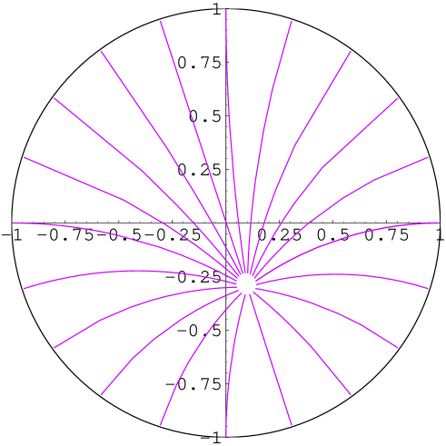
Figure 2: Radial flow for the Gaussian one-scalar model, for charges $(p^{0},p^{1},q_{1},q_{0})=(4,1,1,2)$. All trajectories are attracted to $z_{*}=X^{1}/X^{0}=(1-3i)/10$ at $r=0$.

We shall assume that the charges $(p^{I},q_{I})$ are chosen such that at the attractor point, $Z=Z_{*}\neq 0$, since otherwise the solution becomes singular. Equation (3.27) may be easily integrated near the horizon,

$$\mu=e^{-U}\sim|Z_{*}|/r$$ (3.30)

Defining $z=|Z_{*}|^{2}/r$, it is easy to see that the near-horizon metric becomes $AdS_{2}\times S^{2}$, as in (2.13), where the prefactor $(p^{2}+q^{2})$ is replaced by $|Z_{*}|^{2}$. The Bekenstein-Hawking entropy is one quarter of the horizon area,

$$S_{BH}=\frac{1}{4}\cdot 4\pi\lim_{r\to 0}e^{-2U}r^{2}=\pi|Z_{*}|^{2}$$ (3.31)

This is a function of the electric and magnetic charges only, by virtue of the attractor mechanism, except for possible discrete labels (or “area codes”) corresponding to different basins of attraction.

We shall now put these results in a more manageable form, by making use of some special geometry identities discussed in Section 3. First, using the derived section $U_{i}=(f_{i}^{I},h_{iI})$ defined in (3.4) and the property (3.10), one easily finds

$$\partial_{i}Z=f_{i}^{I}(q_{I}-\bar{\cal N}_{IJ}p^{J})-\frac{1}{2}Z\partial_{i}\mathcal{K}\ ,\quad\partial_{\bar{i}}Z=\frac{1}{2}Z\partial_{\bar{i}}\mathcal{K}$$ (3.32)

so that

$$\frac{\partial_{i}|Z|}{|Z|}=\frac{1}{2}\left(\frac{\partial_{i}Z}{Z}+\frac{\partial_{i}\bar{Z}}{\bar{Z}}\right)=\frac{1}{Z}f_{i}^{I}\left(q_{I}-\bar{\cal N}_{IJ}p^{J}\right)$$ (3.33)

This allows to rewrite (3.28) as

$$r^{2}\frac{dz^{i}}{dr}=-\sqrt{\frac{Z}{\bar{Z}}}e^{U}g^{i\bar{j}}\bar{f}^{J}_{\bar{j}}(q_{I}-{\cal N}_{IJ}p^{J})$$ (3.34)

The stationary value of $z^{i}$ at the horizon is thus obtained by setting the rhs of this equation to zero, i.e.

$$f^{J}_{i}(q_{I}-\bar{\cal N}_{IJ}p^{J})=0$$ (3.35)

The rectangular matrix $f^{I}_{i}$ has a unique zero eigenvector, given by the second equality in (3.12). Hence, (3.35) implies

$$q_{I}-\bar{\cal N}_{IJ}p^{J}=C~{}{\rm Im}{\cal N}_{IJ}X^{J}$$ (3.36)

Contracting either side with $\bar{X}^{I}$ and using the first equation in (3.12) allows to compute the value of $\alpha$,

$$C=-2{\bar{Z}}~{}e^{\mathcal{K}/2}$$ (3.37)

Moreover, using again (3.10), one may rewrite (3.36) and its complex conjugate, equivalently as two real equations

$$p^{I}={\rm Im}(CX^{I})\ ,\quad q_{I}={\rm Im}(CF_{I})$$ (3.38)

while the Bekenstein-Hawking entropy (3.31) is given by

$$S_{BH}=\frac{\pi}{4}|C|^{2}e^{-\mathcal{K}(X,\bar{X})}=\frac{i\pi}{4}|C|^{2}\left(\bar{X}^{I}F_{I}-X^{I}\bar{F}_{I}\right)$$ (3.39)

Making use of the fact that near the horizon, $e^{-U}\sim|Z_{*}|/r$, it is convenient to rescale the holomorphic section $\Omega=(X^{I},F_{I})$ into

$$\begin{pmatrix}Y^{I}\\ G_{I}\end{pmatrix}=2i~{}r~{}e^{\frac{1}{2}\mathcal{K}(X,\bar{X})-U}\sqrt{\frac{\bar{Z}}{Z}}\begin{pmatrix}X^{I}\\ F_{I}\end{pmatrix}$$ (3.40)

in such a way that

$$e^{-\mathcal{K}(Y,\bar{Y})}=4r^{2}e^{-2U}\ ,\quad\arg W(Y)=\pi/2$$ (3.41)

where we defined, in line with (3.3) and (3.15),

$$K(Y,\bar{Y})=\left[i\left(\bar{Y}^{I}G_{I}-Y^{I}\bar{G}_{I}\right)\right]=e^{-\mathcal{K}(Y,\bar{Y})}\ ,\quad W(Y)=q_{I}Y^{I}-p^{I}G_{I}$$ (3.42)

In this fashion, we have incorporated the geometric variable $U$ into the symplectic section $(Y^{I},G_{I})$, and fixed the phase. In this new “gauge”, which amounts to setting $C\equiv i$, (3.38) and (3.31) simplify into

$$\begin{pmatrix}p^{I}\\ q_{I}\end{pmatrix} = {\rm Re}\begin{pmatrix}Y^{I}\\ G_{I}\end{pmatrix}$$ (3.43)

$$S_{BH} = \frac{\pi}{4}K(Y,\bar{Y})=\frac{i\pi}{4}\left[\bar{Y}^{I}G_{I}-Y^{I}\bar{G}_{I}\right]$$ (3.44)

These equations, some times known as “stabilization equations”, are the most convenient way of summarizing the endpoint of the attractor mechanism, as will become apparent in the next subsection.

3.4 Bekenstein-Hawking entropy and Legendre transform

A key observation for later developments is that the Bekenstein-Hawking entropy (3.43) is simply related by Legendre transform to the tree-level prepotential $F$. To see this, note that the first equation in (3.43) is trivially solved by setting $Y^{I}=p^{I}+i\phi^{I}$, where $\phi^{I}$ is real. The entropy is then rewritten as

$$S_{BH} = \frac{i\pi}{4}\left[(Y^{I}-2i\phi^{I})G_{I}-(\bar{Y}^{I}+2i\phi^{I})\bar{G}_{I}\right]$$ (3.45)

$$= \frac{i\pi}{2}\left[F(Y)-\bar{F}(\bar{Y})\right]+\frac{\pi}{2}\phi^{I}\left[G_{I}+\bar{G}_{I}\right]$$ (3.46)

where, in going from the second to the third line, we used the homogeneity of the prepotential, $Y^{I}G_{I}=2F(Y)$. On the other hand, the second stabilization equation yields

$$q_{I}=\frac{1}{2}\left(G_{I}+\bar{G}_{I}\right)=\frac{1}{2i}\left(\frac{\partial F}{\partial\phi^{I}}-\frac{\partial\bar{F}}{\partial\phi^{I}}\right)$$ (3.47)

Thus, defining

$${\cal F}(p^{I},\phi^{I})=-\pi~{}{\rm Im}\left[F(p^{I}+i\phi^{I})\right]$$ (3.48)

the last equation in (3.46) becomes

$$S_{BH}(p^{I},q_{I})=\langle{\cal F}(p^{I},\phi^{I})+\pi~{}\phi^{I}q_{I}\rangle_{\phi^{I}}$$ (3.49)

where the r.h.s. is evaluated at its extremal value with respect to $\phi^{I}$. In usual thermodynamical terms, this implies that ${\cal F}(p^{I},\phi^{I})$ should be viewed as the free energy of an ensemble of black holes in which the magnetic charge $p^{I}$ is fixed, but the electric charge $q_{I}$ is free to fluctuate at an electric potential $\pi\phi^{I}$. The implications of this simple observation will be profound in Section 5.3, when we discuss the higher-derivative corrections to the Bekenstein-Hawking entropy.

Exercise 6

Apply this formalism to show that the entropy of a D0-D4 bound state in type IIA string theory compactified on a Calabi-Yau three-fold, in the large charge regime, is given by

$$S_{BH}=2\pi\sqrt{-C_{ABC}p^{A}p^{B}p^{C}q_{0}}$$ (3.50)

and compare to (2.20).

Exercise 7

Show that the Bekenstein-Hawking entropy (3.44) can be obtained by extremizing

$$\Sigma_{p,q}(Y,\bar{Y})=-\frac{\pi}{4}\left[K(Y,\bar{Y})+2i[W(Y)-\bar{W}(\bar{Y})]\right]$$ (3.51)

with respect to $Y,\bar{Y}$, where $K(Y,\bar{Y})$ and $W(Y)$ are defined in (3.42) [7, 58]. Observe that (3.49) is recovered by extremizing over ${\rm Re}(Y)$.

Exercise 8

Define the Hesse potential $\Sigma(\phi^{I},\chi_{I})$ as the Legendre transform of the topological free energy with respect to the magnetic charges $p^{I}$,

$$\Sigma(\phi^{I},\chi_{I})=\langle\ {\cal F}(p^{I},\phi_{I})+\pi\,\chi_{I}p^{I}\rangle_{p^{I}}$$ (3.52)

Show that the dependence of $\Sigma$ on the electric and magnetic potentials $(\phi^{I},\chi_{I})$ is identical (up to a sign) to that of the black hole entropy $S_{BH}$ on the charges $(p^{I},q_{I})$. Compare to $\Sigma_{p,q}$ in the previous Exercise.

3.5 Very Special Supergravities and Jordan Algebras

In the remainder of this section, we illustrate the previous results on a special class of ${\cal N}=2$ supergravities, whose vector-multiplet moduli spaces are given by symmetric spaces. These are interesting toy models, which arise in various truncations of string compactifications. Moreover, they are related to by analytic continuation to ${\cal N}>2$ theories, which will be further discussed in Section 7.

The simplest way to construct these models is to start from 5 dimensions [59]: the vector multiplets consist of one real scalar for each vector, and their couplings are given by

$$S=\int d^{5}x~{}\sqrt{-g}~{}\left(R-G_{ij}\partial_{\mu}\phi^{i}\partial_{\mu}\phi^{j}\right)-\overset{\circ}{a}_{AB}~{}F^{A}\wedge\star\ F^{B}+\frac{1}{24}\int C_{ABC}~{}A^{A}\wedge F^{B}\wedge F^{C}$$ (3.53)

where the Chern-Simons-type couplings $C_{ABC}$ are constant, for gauge invariance. ${\cal N}=2$ supersymmetry requires the real scalar fields $\phi^{i}$ to take value in the cubic hypersurface ${\cal M}_{5}=\{\xi,N(\xi)=1\}$ in an ambient space $\xi\in\mathbb{R}^{n_{V}+1}$, where

$$N(\xi)=\frac{1}{6}C_{ABC}~{}\xi^{A}~{}\xi^{B}~{}\xi^{C}$$ (3.54)

The metric $G_{ij}$ is then the pull-back of the ambient space metric $a_{AB}d\xi^{A}d\xi^{B}$ to ${\cal M}_{5}$, where

$$a_{AB}=-\frac{1}{2}\partial_{\xi^{A}}\partial_{\xi^{B}}N(\xi)$$ (3.55)

The gauge couplings $\overset{\circ}{a}_{AB}$ are instead given by the restriction of $a_{AB}$ to the hypersurface ${\cal M}_{5}$. Upon reduction from 5 dimensions to 4 dimensions, using the standard Kaluza-Klein ansatz

$$ds^{2}_{5}=e^{2\sigma}(dy+B_{\mu}dx^{\mu})^{2}+e^{-\sigma}g_{\mu\nu}dx^{\mu}dx^{\nu}$$ (3.56)

the Kaluza-Klein gauge field $B_{\mu}$ provides the graviphoton, while the constraint $N(\xi)=1$ is relaxed to $N(\xi)=e^{3\sigma}$. Moreover, $\xi^{A}$ combine with the fifth components $a^{A}$ of the gauge fields $A^{A}$ into complex scalars $t^{A}=a^{A}+i\xi^{A}=X^{A}/X^{0}$, which are the special coordinates of a special Kähler manifold ${\cal M}_{4}$ with prepotential

$$F=N(X^{A})/X^{0}$$ (3.57)

In general, neither ${\cal M}_{5}$ nor ${\cal M}_{4}$ are symmetric spaces. The conditions for ${\cal M}_{5}$ to be a symmetric space were analyzed in [59], and found to have a remarkably simple interpretation in terms of Jordan algebras: these are commutative, non-associative algebras $J$ satisfying the “Jordan identity”

$$x\circ(y\circ x^{2})=(x\circ y)\cdot x^{2}$$ (3.58)

where $x^{2}=x\circ x$ (see e.g. [60] for a nice review).

Exercise 9

Show that the algebra of $n\times n$ hermitean matrices with product $A\circ B=\frac{1}{2}(AB+BA)$ is a Jordan algebra.

Jordan algebras were introduced and completely classified in [61] in an attempt to generalize quantum mechanics beyond the field of complex numbers. The ones relevant here are those which admit a norm $N$ of degree 3 – rather than giving the axioms of the norm, we shall merely list the allowed possibilities:

• One trivial case: $J=\mathbb{R}$, $N(\xi)=\xi^{3}$

• One infinite series: $J=\mathbb{R}\oplus\Gamma$ where $\Gamma$ is the Clifford algebra of $O(1,n-1)$, $N(\xi\oplus\gamma)=\xi\gamma^{a}\gamma^{b}\eta_{ab}$

• Four exceptional cases: $J={\rm Herm}_{3}(\mathbb{D})$, the algebra of $3\times 3$ hermitean matrices $\xi=\begin{pmatrix}\alpha_{1}&x_{3}&\bar{x}_{2}\\ \bar{x}_{3}&\alpha_{2}&x_{1}\\ x_{2}&\bar{x}_{1}&\alpha_{3}\end{pmatrix}$ where $\alpha_{i}$ are real and $x_{i}$ are in one of the four “division algebras” $\mathbb{D}=\mathbb{R},\mathbb{C}$, the quaternions $\mathbb{H}$ or octonions $\mathbb{O}$. In each of these cases, the cubic norm is the “determinant” of $\xi$

  $$N(\xi)=\alpha_{1}\alpha_{2}\alpha_{3}-\alpha_{1}x_{1}\bar{x}_{1}-\alpha_{2}x_{2}\bar{x}_{2}-\alpha_{3}x_{3}\bar{x}_{3}+2{\rm Re}(x_{1}x_{2}x_{3})$$ (3.59)

  For $J_{3}^{\mathbb{C}}$, this is equivalent to the determinant of an unconstrained $3\times 3$ real matrix, and for $J_{3}^{\mathbb{H}}$ to the Pfaffian of a $6\times 6$ antisymmetric matrix.

To each of these Jordan algebras, one may attach several invariance groups, summarized in Table 1:

• $\mbox{Aut}(J)$, the group of automorphisms of $J$, which leaves invariant the structure constants of the Jordan product;

• $\mbox{Str}(J)$, the “structure” group, which leaves invariant the norm $N(\xi)$ up to a rescaling; and the “reduced structure group” $\mbox{Str}_{0}(J)$, where the center has been divided out;

• $\mbox{Conf}(J)$, the “conformal” group, such that the norm of the difference of two elements $N(\xi-\xi^{\prime})$ is multiplied by a product $f(\xi)f(\xi^{\prime})$; as a result, the “cubic light-cone” $N(\xi-\xi^{\prime})=0$ is invariant;

• $\mbox{QConf}(J)$, the “quasi-conformal group”, which we will describe in Section 7.5.

$$\begin{array}[]{|c||c|c|c|c|}\hline\cr J&\mbox{Aut}(J)&\mbox{Str}_{0}(J)&\mbox{Conf}(J)&\mbox{QConf}(J)\\ \hline\cr\hline\cr\mathbb{R}&1&1&Sl(2,\mathbb{R})&G_{2(2)}\\ \hline\cr\mathbb{R}\oplus\Gamma_{n-1,1}&SO(n-1)&SO(n-1,1)&Sl(2)\times SO(n,2)&SO(n+2,4)\\ \hline\cr J_{3}^{\mathbb{R}}&SO(3)&Sl(3,\mathbb{R})&Sp(6)&F_{4(4)}\\ \hline\cr J_{3}^{\mathbb{C}}&SU(3)&Sl(3,\mathbb{C})&SU(3,3)&E_{6(+2)}\\ \hline\cr J_{3}^{\mathbb{H}}&USp(6)&SU^{*}(6)&SO^{*}(12)&E_{7(-5)}\\ \hline\cr J_{3}^{\mathbb{O}}&F_{4}&E_{6(-26)}&E_{7(-25)}&E_{8(-24)}\\ \hline\cr\end{array}$$

Table 1: Invariance groups associated to degree 3 Jordan algebras. The lower $4\times 4$ part is known as the “Magic Square”, due to its symmetry along the diagonal [62].

In the case ii) above, $\mbox{Aut}(J),\mbox{Str}(J)$ and $\mbox{Conf}(J)$ are just the orthogonal group $SO(n-1)$, Lorentz group $SO(n-1,1)$ and conformal group $SO(n,2)$ times an extra $Sl(2)$ factor.

The relevance of these groups for physics is as follows: choosing $N(\xi)$ in (3.54) to be equal to the norm form of a Jordan algebra $J$, the vector-multiplet moduli spaces for the resulting ${\cal N}=2$ supergravity in $D=5$ and $D=4$ are symmetric spaces

$${\cal M}_{5}=\frac{\mbox{Str}_{0}(J)}{\mbox{Aut}(J)}\ ,\quad{\cal M}_{4}=\frac{\mbox{Conf}(J)}{\widetilde{\mbox{Str}}_{0}(J)\times U(1)}\ ,\quad$$ (3.60)

where $\widetilde{\mbox{Str}}_{0}(J)$ denotes the compact real form of $\mbox{Str}_{0}(J)$. In either case, the group in the denominator is the maximal subgroup of the one in the numerator, which guarantees that the quotient has positive definite signature. The resulting spaces are shown in Table 2, together with the ones which appear upon reduction to $D=3$ on a space-like and time-like direction respectively, to be discussed in Section 7.5 below. The first column indicates the number of supercharges in the corresponding supergravity: the above discussion applies strictly speaking to cases with 8 supercharges (i.e. ${\cal N}=2$ supersymmetry in 4 dimensions), but other cases can also be reached with similar techniques, using different real forms of the Jordan algebras above.

$$\begin{array}[]{|c|c|c|c|c|c|}\hline\cr Q&J&D=5&D=4&D=3&D=3^{*}\\ \hline\cr\hline\cr 8&&&\frac{SU(n,1)}{SU(n)\times U(1)}&\frac{SU(n+1,2)}{SU(n+1)\times SU(2)\times U(1)}&\frac{SU(n+1,2)}{SU(n,1)\times Sl(2)\times U(1)}\\ \hline\cr 8&\Gamma_{n-1,1}&\mathbb{R}\times\frac{SO(n-1,1)}{SO(n-1)}&\frac{SO(n,2)}{SO(n)\times SO(2)}\times\frac{Sl(2)}{U(1)}&\frac{SO(n+2,4)}{SO(n+2)\times SO(4)}&\frac{SO(n+2,4)}{SO(n,2)\times SO(2,2)}\\ \hline\cr 8&&&\frac{Sl(2)}{U(1)}&\frac{SU(2,1)}{SU(2)\times U(1)}&\frac{SU(2,1)}{Sl(2)\times U(1)}\\ \hline\cr 8&\mathbb{R}&\varnothing&\frac{Sl(2)}{U(1)}&\frac{G_{2(2)}}{SO(4)}&\frac{G_{2(2)}}{SO(2,2)}\\ \hline\cr 8&J_{3}^{\mathbb{R}}&\frac{Sl(3)}{SO(3)}&\frac{Sp(6)}{SU(3)\times U(1)}&\frac{F_{4(4)}}{USp(6)\times SU(2)}&\frac{F_{4(4)}}{Sp(6)\times Sl(2)}\\ \hline\cr 8&J_{3}^{\mathbb{C}}&\frac{Sl(3,C)}{SU(3)}&\frac{SU(3,3)}{SU(3)\times SU(3)\times U(1)}&\frac{E_{6(+2)}}{SU(6)\times SU(2)}&\frac{E_{6(+2)}}{SU(3,3)\times Sl(2)}\\ \hline\cr 24&J_{3}^{\mathbb{H}}&\frac{SU^{*}(6)}{USp(6)}&\frac{SO^{*}(12)}{SU(6)\times U(1)}&\frac{E_{7(-5)}}{SO(12)\times SU(2)}&\frac{E_{7(-5)}}{SO^{*}(12)\times Sl(2)}\\ \hline\cr 8&J_{3}^{\mathbb{O}}&\frac{E_{6(-26)}}{F_{4}}&\frac{E_{7(-25)}}{E_{6}\times U(1)}&\frac{E_{8(-24)}}{E_{7}\times SU(2)}&\frac{E_{8(-24)}}{E_{7(-25)}\times Sl(2)}\\ \hline\cr 10&&&&\frac{Sp(2n,4)}{Sp(2n)\times Sp(4)}&\\ \hline\cr 12&&&&\frac{SU(n,4)}{SU(n)\times SU(4)}&\\ \hline\cr 16&\Gamma_{n-5,5}&\mathbb{R}\times\frac{SO(n-5,5)}{SO(n-5)\times SO(5)}&\frac{Sl(2)}{U(1)}\times\frac{SO(n-4,6)}{SO(n-4)\times SO(6)}&\frac{SO(n-2,8)}{SO(n-2)\times SO(8)}&\frac{SO(n-2,8)}{SO(n-4,2)\times SO(2,2)}\\ \hline\cr 18&&&&\frac{F_{4(-20)}}{SO(9)}&\\ \hline\cr 20&M_{1,2}(\mathbb{O})&&\frac{SU(5,1)}{SU(5)\times U(1)}&\frac{E_{6(-14)}}{SO(10)\times SO(2)}&\frac{E_{6(-14)}}{SO^{*}(10)\times SO(2)}\\ \hline\cr 32&J_{3}^{\mathbb{O}_{s}}&\frac{E_{6(6)}}{USp(8)}&\frac{E_{7(7)}}{SU(8)}&\frac{E_{8(8)}}{SO(16)}&\frac{E_{8(8)}}{SO^{*}(16)}\\ \hline\cr\end{array}$$

Table 2: Moduli spaces for supergravities with symmetric moduli spaces. The last column refers to the reduction from 4 dimensions to 3 along a time-like direction, which will become relevant in Section 7.

The $\mbox{Str}_{0}(J)$ invariance of the metric on ${\cal M}_{5}$ is indeed obvious from (3.55) above. The $\mbox{Conf}(J)$ invariance of the metric on the special Kähler space ${\cal M}_{4}$ is manifest too, since the Kähler potential following from (3.57) is the proportional to the log of the “cubic light-cone”,

$$\mathcal{K}(z,\bar{z})=-\log N(z_{i}-\bar{z}_{i})\ ,$$ (3.61)

invariant under $\mbox{Conf}(J)$ up to Kähler transformations. Such special Kähler spaces are known as hermitean symmetric tube domains, and are higher-dimensional analogues of Poincaré’s upper half plane.

It should be pointed out that there also exist $D=4$ SUGRAs with symmetric moduli space which do not descend from 5 dimensions: they may be described by a generalization of Jordan algebras known as “Freudenthal triple systems”, but we will not discuss them in any detail here. Similarly, there exist $D=3$ supergravity theories with symmetric moduli spaces which cannot be lifted to 4 dimensions.

In general, it is not known whether these very special supergravities arise as the low-energy limit of string theory. All except the exceptional $J_{3}^{\mathbb{O}}$ case can be obtained formally by truncation of $\mathcal{N}=8$ supergravity, but it is in general unclear how to consistently enforce this truncation. A notable exception is the case based on $J=\Gamma_{9,1}$, which is realized in type IIA string theory compactified on a freely acting orbifold of $K3\times T^{2}$, or a CHL orbifold of the heterotic string on $T^{6}$ [64]. The model with $J=J_{3}^{\mathbb{C}}$ arises in the untwisted sector of type IIA compactified on the “Z-manifold” $T^{6}/\mathbb{Z}_{3}$ [65], but there are also massless fields from the twisted sector. We shall mostly use these theories at toy models in the sequel, and assume that discrete subgroups $\mbox{Str}_{0}(J,\mathbb{Z})$ and $\mbox{Conf}(J,\mathbb{Z})$ remain as quantum symmetries of the full quantum theory, if it exists.

3.6 Bekenstein-Hawking Entropy in Very Special Supergravities

As an illustration of the simplicity of these models, we shall now proceed and compute the Bekenstein-Hawking entropy for BPS black holes with arbitrary charges, following [8]. A key property which renders the computation tractable is the fact that the prepotential (3.57) obtained from any Jordan algebra is invariant (up to a sign) under Legendre transform in all variables, namely

$$\langle N(X^{A})/X^{0}+X^{A}Y_{A}+X^{0}Y_{0}\rangle_{X^{I}}=-N(Y)/Y^{0}$$ (3.62)

Exercise 10

Show that (3.62) is equivalent to the “adjoint identity” for Jordan algebras, $X^{\sharp\sharp}=N(X)X$ where $X^{\sharp}_{A}=\frac{1}{2}C_{ABC}X^{B}X^{C}$ is the “quadratic map” from $J$ to its dual.

In fact, just imposing (3.62) leads to the same classification i),ii),iii) as above. This was shown independently in [66], as a first step in finding cubic analogues of the Gaussian, invariant under Fourier transform (see [67] for a short account).

Exercise 11

Check by explicit computation that for the “STU” model, $(1/X^{0})e^{N(X^{A})/X^{0}}$ is invariant under Fourier transform, namely

$$\int\frac{dX^{0}dX^{1}dX^{2}dX^{3}}{X^{0}}\exp\left[i\frac{X^{1}X^{2}X^{3}}{\hbar X^{0}}+iX^{I}Y_{I}\right]=\frac{\hbar}{Y^{0}}\exp\left[{i\hbar}\frac{Y_{1}Y_{2}Y_{3}}{Y_{0}}\right]$$ (3.63)

Conclude that the semi-classical approximation to this integral is exact. Hint: perform the integral over $X^{1},X^{2},X^{0},X^{3}$ in this order.

In order to compute the Bekenstein-Hawking entropy, we start from the “free energy” (3.48)

$${\cal F}(p,\phi)=\frac{\pi}{(p^{0})^{2}+(\phi^{0})^{2}}\left\{p^{0}\left[\phi^{A}p_{A}^{\sharp}-N(\phi)\right]+\phi^{0}\left[p^{A}\phi_{A}^{\sharp}-N(p)\right]\right\}$$ (3.64)

To eliminate the quadratic term in $\phi^{A}$, let us change variables to

$$x^{A}=\phi^{A}-\frac{\phi^{0}}{p^{0}}p^{A}\ ,\quad x^{0}=[(p^{0})^{2}+(\phi^{0})^{2}]/p^{0}$$ (3.65)

Moreover, we introduce an auxiliary variable $t$, such that, upon eliminating $t$, we recover (3.64):

$$S_{BH}=\pi\langle-\frac{N(x^{A})}{x^{0}}+\frac{p_{A}^{\sharp}+p^{0}q_{A}}{p^{0}}x^{A}-\frac{t}{4}\left(\frac{x^{0}}{p^{0}}-1\right)-\frac{(2N(p)+p^{0}p^{I}q_{I})^{2}}{t\ (p^{0})^{2}}\rangle_{\{x^{I},t\}}$$ (3.66)

Extremizing over $x^{I}$ now amounts to Legendre transforming $N(x)/x^{0}$, which according to (3.62) reproduces $-N(y)/y^{0}$ where $y^{I}$ are the coefficients of the linear terms in $x^{I}$, so

$$S_{BH}=\pi\langle 4\frac{N[p_{A}^{\sharp}+p^{0}q_{A}]}{(p^{0})^{2}t}-\frac{[2N(p)+p^{0}p^{I}q_{I}]^{2}}{t\ (p^{0})^{2}}+\frac{t}{4}\rangle_{t}$$ (3.67)

Finally, extremizing over $t$ leads to

$$S_{BH}=\frac{\pi}{p^{0}}\sqrt{4N[p_{A}^{\sharp}+p^{0}q_{A}]-[2N(p)+p^{0}p^{I}q_{I}]^{2}}$$ (3.68)

The pole at $p^{0}=0$ is fake: upon Taylor expanding $N[p_{A}^{\sharp}+p^{0}q_{A}]$ in the numerator and further using the homogeneity of $N$, its coefficient cancels. The final result gives the entropy as the square root of a quartic polynomial in the charges,

$$S_{BH}=\pi\sqrt{I_{4}(p^{I},q_{I})}$$ (3.69)

where

$$I_{4}(p^{I},q_{I})=4p^{0}N(q_{A})-4q_{0}N(p^{A})+4q^{A}_{\sharp}p_{A}^{\sharp}-(p^{0}q_{0}+p^{A}q_{A})^{2}$$ (3.70)

The fact that this quartic polynomial is invariant under the linear action of the four-dimensional “U-duality” group $\mbox{Conf}(J)$ on the symplectic vector of charges $(p^{I},q_{I})$, follows from Freudenthal’s “triple system construction”. Several examples are worth mentioning:

• For the “STU” model with $N(\xi)=\xi^{1}\xi^{2}\xi^{3}$, the electric-magnetic charges transform as a $(2,2,2)$ of $\mbox{Conf}(J)=Sl(2)^{3}$, so can be viewed as sitting at the 8 corners of a cube; the quartic invariant is known as Cayley’s “hyperdeterminant”

  $$I_{4}=-\frac{1}{2}\epsilon^{AB}\epsilon^{CD}\epsilon^{ab}\epsilon^{cd}\epsilon^{\alpha\gamma}\epsilon^{\beta\delta}q_{Aa\alpha}Q_{Bb\beta}Q_{Cc\gamma}Q_{Dd\delta}$$ (3.71)

  This has recently been related to the “three-bit entanglement” in quantum information theory [68, 69, 70].

• More generally, for the infinite series, where the charges transform as a $(2,n)$ of $Sl(2)\times SO(2,n)$, the quartic invariant is

  $$I_{4}=(\vec{q}_{e}\cdot\vec{q}_{e})(\vec{q}_{m}\cdot\vec{q}_{m})-(\vec{q}_{e}\cdot\vec{q}_{m})^{2}$$ (3.72)

  Up to a change of signature of the orthogonal group, this is the quartic invariant which appears in the entropy of 1/4-BPS black holes in ${\cal N}=4$ theories (2.22).

• In the exceptional $J_{3}^{\mathbb{O}}$ case, $I_{4}$ is the quartic invariant of the 56 representation of $E_{7(-25)}$. Replacing $\mathbb{O}$ by the split octonions $\mathbb{O}_{s}$, one obtains the quartic invariant of $E_{7(7)}$, which appears in the entropy $S=\pi\sqrt{I_{4}}$ of 1/8-BPS states in ${\cal N}=8$ supergravity [71],

  $$I_{4}(P,Q)=-\mbox{Tr}(QPQP)+\frac{1}{4}\left(\mbox{Tr}QP\right)^{2}-4\left[\mbox{Pf}(P)+\mbox{Pf}(Q)\right]$$ (3.73)

  where the entries in the antisymmetric $8\times 8$ matrices $Q$ and $P$ may be identified as [8]:

  $$Q=\begin{pmatrix}[D2]^{ij}&[F1]^{i}&[kkm]^{i}\\ -[F1]^{i}&0&[D6]\\ -[kkm]^{i}&-[D6]&0\end{pmatrix}\ ,\quad P=\begin{pmatrix}[D4]_{ij}&[NS5]_{i}&[kk]_{i}\\ -[NS5]_{i}&0&[D0]\\ -[kk]_{i}&-[D0]&0\end{pmatrix}\ ,\quad$$ (3.74)

  Here, $[D2]^{ij}$ denotes a D2-brane wrapped along the directions $ij$ on $T^{6}$, $[D4]_{ij}$ a D4-branes wrapped on all directions but $ij$, $[kk]_{i}$ a momentum state along direction $i$, $[kkm]^{i}$ a Kaluza-Klein 5-monopole localized along the direction $i$ on $T^{6}$, $[F1]^{i}$ a fundamental string winding along direction $i$, and $[NS5]_{i}$ a NS5-brane wrapped on all directions but $i$.

Exercise 12

Show that in the ${\cal N}=4$ truncation where only the $[F1],[kk],[NS5],[kkm]$ charges are retained, (3.73) reduces to the quartic invariant (2.22) under $Sl(2)\times SO(6,6)$. Similarly, in the ${\cal N}=2$ truncation where only $[D0],[D2],[D4],[D6]$ are kept, show that one obtains the quartic invariant of a spinor of $SO^{*}(12)$, based on the Jordan algebra $J_{3}^{\mathbb{H}}$.

The intermediate equation (3.67) also has an interesting interpretation: it is recognized as $1/p^{0}$ times the entropy $S_{5D}=\pi\sqrt{N(Q)-J^{2}}$ of a five-dimensional BPS black hole with electric charge and angular momentum

$$Q_{A} = p^{0}q_{A}+C_{ABC}p^{B}p^{C}$$ (3.75)

$$2J_{L} = (p^{0})^{2}q_{0}+p^{0}p^{A}q_{A}+2N(p)$$ (3.76)

The interpretation of these relations is as follows: when the D6-brane charge $p^{0}$ is non-zero, the 4D black hole in Type IIA compactified on $\tilde{Y}$ may be lifted to a 5D black hole in M-theory on $\tilde{Y}\times TN_{p^{0}}$, where $TN$ denotes the 4-dimensional Euclidean Taub-NUT space with NUT charge $p^{0}$; at spatial infinity, this asymptotes to $\mathbb{R}^{3}\times S^{1}$, where the circle is taken to be the M-theory direction. Translations along this direction at infinity, conjugate to the D0-brane charge $q_{0}$, become $SU(2)$ rotations at the center of $TN$, where the black hole is assumed to sit. The remaining factors of $p^{0}$ are accounted for by taking into account the $\mathbb{R}^{4}/\mathbb{Z}_{p^{0}}$ singularity at the origin of $TN$ [72]. The formulae (3.75) extend this lift to an arbitrary choice of charges, in a manifestly duality invariant manner.

Exercise 13

Using the fact that the degeneracies of five-dimensional black holes on $K3\times S^{1}$ are given by the Fourier coefficients of the elliptic genus of ${\rm Hilb}(K3)$, equal to $1/\Phi_{10}$, show that the DVV conjecture (2.23) holds for at least one U-duality orbit of 4-dimensional dyons in type II/$K3\times T^{2}$ with one unit of D6-brane and some amout of D0,D2-brane charge. You might want to seek help from [42].

4 Topological String Primer

In the previous sections, we were concerned exclusively with low energy supergravity theories, whose Lagrangian contains at most two-derivative terms. This is sufficient in the limit of infinitely large charges, but not for more moderate values, where higher-derivative corrections start playing a role. In this section, we give a self-contained introduction to topological string theory, which offers a practical way of to compute an infinite series of such corrections. Sections 4.1 and 4.2 draw heavily from [73]. Other valuable reviews of topological string theory include [74, 75, 76, 77, 78].

4.1 Topological Sigma Models

Type II strings compactified on a Kähler manifold $X$ of complex dimension $d$ are described by a $N=(2,2)$ sigma model

$$S=2t\int d^{2}z\left(g_{i\bar{j}}\partial\phi^{i}\bar{\partial}\phi^{\bar{j}}+g_{i\bar{j}}\bar{\partial}\phi^{i}\partial\phi^{\bar{j}}+i\psi^{\bar{i}}_{-}D\psi_{-}^{i}g_{i\bar{i}}+i\psi^{\bar{i}}_{+}\bar{D}\psi_{+}^{i}g_{i\bar{i}}+R_{i\bar{i}j\bar{j}}\psi_{+}^{i}\psi_{+}^{\bar{i}}\psi_{-}^{j}\psi_{-}^{\bar{j}}\right)$$ (4.1)

where $\phi$ is a map from a two-dimensional genus $g$ Riemann surface $\Sigma$ to $X$, $\psi_{\pm}^{i}$ is a section of $K^{1/2}_{\pm}\otimes\phi^{*}(T^{1,0}X)$, $\psi_{\pm}^{\bar{i}}$ is a section of $K^{1/2}_{\pm}\otimes\phi^{*}(T^{0,1}X)$, and we denoted by $K_{+}$ the canonical bundle on $\Sigma$ (i.e. the bundle of (1,0) forms) and $K_{-}$ the anti-canonical bundle (of (0,1) forms). The factor of $t$ (the string tension) is to keep track on the dependence on the overall volume of $X$.

This model is invariant under $N=(2,2)$ superconformal transformations generated with sections $\alpha_{\pm}$ and $\tilde{\alpha}_{\pm}$ of $K_{\pm}^{1/2}$, acting e.g. as

$$\delta\phi^{i}=i(\alpha_{-}\psi_{+}^{i}+\alpha_{+}\psi_{-}^{i})\ ,\quad\delta\phi^{\bar{i}}=i(\tilde{\alpha}_{-}\psi_{+}^{\bar{i}}+\tilde{\alpha}_{+}\psi_{-}^{\bar{i}})$$ (4.2)

This implies chirally conserved supercurrents $G^{\pm}$ of conformal dimension 3/2, which together with $T$ and the current $J$ generate the ${\cal N}=2$ superconformal algebra,

$$G^{+}(z)~{}G^{-}(0) = \frac{2c}{3}\frac{1}{z^{2}}+\left(\frac{2J}{z^{2}}+\frac{\partial J+2T}{z}\right)+{\rm reg}$$ (4.3)

$$J(z)J(0) = \frac{c}{3}\frac{1}{z^{2}}+{\rm reg}$$ (4.4)

The current $J$ appearing in the OPE (4.3) generates a $U(1)$ symmetry, such that $G_{\pm}$ have charge $Q=\pm 1$ while $T$ and $J$ are neutral. In the (doubly degenerate) Ramond sectors $R_{\pm}$, the zero-modes of the supercurrents generate a supersymmetry algebra

$$(G_{0}^{+})^{2}=(G_{0}^{-})^{2}=0\ ,\quad\left\{G_{0}^{+},G_{0}^{-}\right\}=2\left(L_{0}^{R_{\pm}}-\frac{c}{24}\right)$$ (4.5)

Unitarity forces the right-hand side to be positive on any state. Moreover, the ${\cal N}=2$ algebra admits an automorphism known as spectral flow, which relates the NS and R sectors:

$$J_{0}^{R_{\pm}}=J_{0}^{NS}\mp\frac{c}{6}\ ,\quad L_{0}^{R_{\pm}}=L_{0}^{NS}\mp\frac{1}{2}J_{0}^{NS}+\frac{c}{24}$$ (4.6)

The unitary bound $\Delta\geq c/24$ in the R sector therefore implies a bound $\Delta\geq|Q|/2$ after spectral flow. States which saturate this bound have no short distance singularities when brought together, and thus form a ring under OPE, known as the chiral ring of the ${\cal N}=2$ SCFT. Applying the spectral flow twice maps the NS sector back to itself, with $(\Delta,Q)\to(\Delta-Q+\frac{c}{6},Q\mp\frac{c}{3})$. In particular, the NS ground state is mapped to a state with $(\Delta,q)=(\frac{c}{6},\mp\frac{c}{3})$ in the chiral ring. For a Calabi-Yau three-fold, starting from the identity we thus obtain two R states with $(\Delta,q)=(3/8,\pm 3/2)$, and one NS state with $(\Delta,q)=(3/2,\pm 3)$: these are identified geometrically as the covariantly constant spinor and the holomorphic $(3,0)$ form, respectively.

The spectral flow (4.6) above can be used to “twist” the ${\cal N}=2$ sigma model into a topological sigma model: for this, bosonize the $U(1)$ current $J=i\sqrt{3}\partial H$, so that the spectral flow operator becomes

$$\Sigma_{\pm}=\exp\left(\pm i\frac{\sqrt{3}}{2}H(z)\right)$$ (4.7)

with $(\Delta=3/8,Q=\pm 3/2)$. The topological twist then amounts to adding a background charge $\pm\int\frac{\sqrt{3}}{2}H~{}R^{(2)}$: its effect is to change the two-dimensional spin $L_{0}$ into a linear combination $L_{0}\mp\frac{1}{2}J_{0}$ of the spin and the $U(1)$ charge. Under this operation, choosing the $+$ sign, $\psi_{+}^{i}$ becomes a section of $\phi^{*}(T^{1,0}X)$, i.e. a worldsheet scalar, whereas $\psi_{+}^{\bar{i}}$ becomes a section of $K_{+}\otimes\phi^{*}(T^{0,1}X)$, i.e. a worldsheet one-form; simultaneously, the supersymmetry parameters $\alpha_{-}$ and $\tilde{\alpha}_{-}$ become a scalar and a section of $K^{-1}$, respectively. Alternatively, we may choose the $-$ sign in (4.6), where instead $\psi_{+}^{i}$ would become a section of $K_{+}\otimes\phi^{*}(T^{1,0}X)$, while $\psi_{+}^{\bar{i}}$ would turn into a worldsheet scalar. In either case, it is necessary that the canonical bundle $K$ be trivial, in order for that the correlation functions be unaffected by the twist : this is achieved only when computing particular “topological amplitudes” in string theory, which we will discuss in Section 5.1.

Since the sigma model (4.1) has $(2,2)$ superconformal invariance, it is possible to twist both left and right-movers by a spectral flow of either sign. Only the relative choice of sign is important, leading to two very distinct-looking theories, which we discuss in turn:

4.1.1 Topological A-model

Here, both $\psi^{i}_{+}$ and $\psi_{-}^{\bar{i}}$ are worldsheet scalars, and can be combined in a scalar $\chi\in\phi^{*}(TX)$. On the other hand, $\psi^{i}_{-}$ and $\psi^{\bar{i}}_{+}$ become (0,1) and (1,0) forms $\psi^{i}_{\bar{z}}$ and $\psi^{\bar{i}}_{z}$ on the worldsheet. The action is rewritten as

$$S=2t\int d^{2}z\left(g_{i\bar{j}}\partial\phi^{i}\bar{\partial}\phi^{\bar{j}}+g_{i\bar{j}}\bar{\partial}\phi^{i}\partial\phi^{\bar{j}}+i\psi^{\bar{i}}_{z}\bar{D}\chi^{i}g_{i\bar{i}}+i\psi^{\bar{i}}_{\bar{z}}D\chi^{\bar{i}}g_{i\bar{i}}-R_{i\bar{i}j\bar{j}}\psi^{i}_{\bar{z}}\psi^{\bar{i}}_{z}\chi^{j}\chi^{\bar{j}}\right)$$ (4.8)

It allows for a conserved “ghost” charge where $[\phi]=0,[\chi]=1,[\psi]=-1$, and is invariant under the scalar nilpotent operator $Q=G_{+}$,

$$\{Q,\phi^{I}\}=\chi^{I}\ ,\quad\{Q,\chi^{I}\}=0\ ,\{Q,\psi^{i}_{\bar{z}}\}=i\bar{\partial}\phi^{i}-\chi^{j}\Gamma^{i}_{jk}\psi_{\bar{z}}^{k}$$ (4.9)

The action (4.8) is in fact $Q$-exact, up to a total derivative term proportional to the pull-back of the Kähler form $\omega_{K}=ig_{i\bar{j}}d\phi^{i}\wedge d\phi^{\bar{j}}$, complexified into $J=B+i\omega_{K}$ by including the coupling to the NS two-form:

$$S=-i\{Q,V\}-t\int_{\Sigma}\phi^{*}(J)$$ (4.10)

where $V$ is the “gauge fermion”

$$V=t\int d^{2}z~{}g_{i\bar{j}}\left(\psi^{i}_{\bar{z}}\partial\phi^{\bar{j}}+\psi^{\bar{j}}_{z}\bar{\partial}\phi^{i}\right)$$ (4.11)

This makes it clear that the theory is independent of the worldsheet metric, since the energy momentum tensor is $Q$-exact:

$$T_{\alpha\beta}=\{Q,b_{\alpha\beta}\}\ ,\quad b_{\alpha\beta}=\frac{\partial V}{\partial g^{\alpha\beta}}$$ (4.12)

Moreover, the string tension $t$ appears only in the total derivative term so, in a sector with fixed homology class $\int_{\Sigma}\phi^{*}(J)$, the semi-classical limit $t\to 0$ is exact. The path integral thus localizes to the moduli space of $Q$-exact configurations,

$$\partial_{\bar{z}}\phi^{i}=0,\quad\partial_{z}\phi^{\bar{i}}=0$$ (4.13)

i.e. holomorphic maps from $\Sigma$ to $X$. Moreover, the local observables of the A-model $O_{\cal W}=W_{I_{1}\dots I_{n}}\chi^{I_{1}}\dots\chi^{I_{n}}$, where $W_{I_{1}\dots I_{n}}d\phi^{I_{1}}\dots d\phi^{I_{n}}$ is a differential form on $X$ of degree $n$, are in one-to-one correspondence with the de Rham cohomology of $X$, since $\{Q,{\cal O}_{W}\}=-{\cal O}_{dW}$. Due to an anomaly in the conservation of the ghost charge, correlators of $l$ observables vanish unless

$$\sum_{k=1}^{l}{\rm deg}(W_{k})=2d(1-g)+2\int_{\Sigma}\phi^{*}(c_{1}(X))$$ (4.14)

The last term vanishes when the Calabi-Yau condition $c_{1}(X)$ is obeyed. For Calabi-Yau threefolds, at genus 0 the only correlator involves three degree 2 forms,

$$\langle{\cal O}_{W_{1}}{\cal O}_{W_{2}}{\cal O}_{W_{3}}\rangle=\int W_{1}\wedge W_{2}\wedge W_{3}+\sum_{\beta\in H^{2+}(X)}~{}e^{-t\int_{\beta}J}~{}\int_{\beta}W_{1}~{}\int_{\beta}W_{2}~{}\int_{\beta}W_{3}$$ (4.15)

At genus 1, only the vacuum amplitude, known as the elliptic genus of $X$ is non-zero. In Section 4.2, we will explain the prescription to construct non-zero amplitudes at any genus, by coupling to topological gravity.

4.1.2 Topological B-model

The other inequivalent choice consists in twisting $\psi^{\bar{i}}_{\pm}$ into worldsheet scalars valued in $TX^{0,1}$, while $\psi_{+}^{i}$ and $+\psi_{-}^{i}$ are $(0,1)$ and $(1,0)$ forms valued in $TX^{1,0}$. Defining $\eta^{\bar{i}}=\psi_{+}^{\bar{i}}+\psi_{-}^{\bar{i}}$, $\theta_{i}=g_{i\bar{i}}(\psi_{+}^{\bar{i}}-\psi_{-}^{\bar{i}}$, and taking $\psi^{i}_{\pm}$ as the two components of a one-form $\rho^{i}$, the action may be rewritten as

$$S=i~{}t\{Q,V\}+t~{}W$$ (4.16)

where

$$V = \int_{\Sigma}d^{2}z~{}g_{i\bar{j}}\left(\rho^{i}_{z}\bar{\partial}\phi^{\bar{j}}+\rho^{i}_{z}\bar{\partial}\phi^{\bar{j}}\right)$$ (4.17)

$$W = -\int_{\Sigma}d^{2}z~{}\left(\theta_{i}D\rho^{i}+\frac{i}{2}R_{i\bar{i}j\bar{j}}~{}\rho^{i}\wedge\rho^{j}~{}\eta^{\bar{i}}\theta_{k}g^{k\bar{j}}\right)$$ (4.18)

and the nilpotent operator $Q=G_{-}$ acts as

$$\{Q,\phi^{i}\}=0\ ,\quad\{Q,\phi^{\bar{i}}\}=-\eta^{\bar{i}}\ ,\quad\{Q,\eta^{\bar{i}}\}=\{Q,\theta_{i}\}=0\ ,\quad\{Q,\rho^{i}\}=-id\phi^{i}$$ (4.19)

Again, the energy-momentum tensor is $Q$-exact, so that the model is topological. It is also independent of the Kähler structure of $X$, and has a trivial dependence on $t$, since (apart from contributions from the $Q$-exact term) $t$ may be reabsorbed by rescaling $\theta\to\theta/t$. The semi-classical limit $t\to\infty$ is therefore again exact, and the path integral localizes on the fixed points of $Q$, which are now constant maps, $d\phi^{i}=0$. After localization, the path integral then reduces to an integral over $X$.

The observables of the B-model are in one-to-one correspondence with degree $(p,q)$ polyvector fields

$$V=V_{\bar{i}_{1}\dots\bar{i}_{p}}^{j_{1}\dots j_{q}}~{}d\bar{z}^{\bar{i}_{1}}\dots d\bar{z}^{\bar{i}_{p}}~{}\partial_{z^{j_{1}}}\dots\partial_{z^{j_{q}}}\in H^{p}\left(X,\Lambda^{q}T^{1,0}X\right)$$ (4.20)

via $d\bar{z}^{\bar{i}}\sim\eta^{\bar{i}},\partial_{z^{j}}\sim\theta_{j}$, since $\{Q,{\cal O}_{V}\}=-{\cal O}_{\bar{\partial}V}$. There are now two conserved ghost charges, and the anomaly in the ghost number conservation requires that

$$\sum_{k=1}^{l}p_{k}=\sum_{k=1}^{l}q_{k}=d(1-g)$$ (4.21)

For example, at genus 0, the only vanishing correlator on a Calabi-Yau three-fold involves three (1,1) polyvector fields $V^{i}_{\bar{j}}$. Using the holomorphic $(3,0)$ form, these are related to $(2,1)$ forms $\Omega_{ijl}V^{l}_{\bar{k}}$ parameterizing the complex structure of $X$. The three-point function is

$$\langle{\cal O}_{V_{1}}{\cal O}_{V_{2}}{\cal O}_{V_{3}}\rangle=\int_{X}~{}V^{i_{1}}_{\bar{j}_{1}}~{}V^{i_{2}}_{\bar{j}_{2}}~{}V^{i_{3}}_{\bar{j}_{3}}\Omega_{i_{1}i_{2}i_{3}}~{}d\bar{z}^{\bar{j}_{1}}\wedge d\bar{z}^{\bar{j}_{2}}\wedge d\bar{z}^{\bar{j}_{3}}\wedge\Omega$$ (4.22)

giving access to the third derivative of the prepotential.

4.2 Topological Strings

Due to the conservation of the ghost number, we have seen that, from the sigma model alone, the only non-vanishing topological correlators are the three-point function on the sphere, and the vacuum amplitude on the torus. It turns out that the coupling to topological gravity allows to lift this constraint, and define arbitrary $n$-point amplitudes at any genus.

Recall that in bosonic string theory, genus $g$ amplitudes are obtained by introducing $6g-6$ insertions of the dimension 2 ghost (or, rather, “antighost”) $b$ of diffeomorphism invariance, folded with Beltrami differentials $\mu_{k}\in H^{1}(\Sigma,T^{1,0}\Sigma)$:

$$F_{g}=\int_{{\cal M}_{g}}~{}\langle\prod_{k=1}^{6g-6}(b,\mu_{k})\rangle$$ (4.23)

where

$$(b,\mu)=\int_{\Sigma}d^{2}z\left[b_{zz}\mu_{\bar{z}}^{z}+b_{\bar{z}\bar{z}}~{}\bar{\mu}_{z}^{\bar{z}}\right]$$ (4.24)

This effectively produces the Weil-Peterson volume element on the moduli space ${\cal M}_{g}$ of complex structures on the genus $g$ Riemann surface $\Sigma$ (compactified à la Deligne-Mumford). Since $b$ has ghost number $-1$, this exactly compensates the anomalous background charge.

After the topological twist, which identifies the BRST charge $Q$ with (say) $G_{+}$, it is natural to identify $b$ with $G_{-}$, in such a way that the energy-momentum tensor is given by $T=\{Q,b\}=\{G_{+},G_{-}\}$. Hence, the genus $g$ vacuum topological amplitude may be written as

$$F_{g}=\int_{{\cal M}_{g}}~{}\langle\prod_{k=1}^{3g-3}(G_{-},\mu_{k})~{}(G_{\pm},\bar{\mu}_{k})\rangle$$ (4.25)

where the upper (resp., lower) sign corresponds to the A-model (resp., B-model). Scattering amplitudes may be obtained by inserting vertex operators with zero ghost number; these may be obtained by “descent” from a ghost number 2 operator ${\cal O}^{(0)}$,

$$d{\cal O}^{(0)}=\{Q,{\cal O}^{(1)}\}\ ,\quad d{\cal O}^{(1)}=\{Q,{\cal O}^{(2)}\}\$$ (4.26)

Prominent examples of ${\cal O}^{(0)}$ are of course $W_{i\bar{i}}\chi^{i}\chi^{\bar{i}}$ in the A-model, and $V_{j}^{\bar{i}}\eta^{\bar{i}}\theta_{j}$ in the B-model. These describes the deformations of the Kähler and complex structures, respectively. Arbitrary numbers of integrated vertex operators $\int d^{2}z~{}{\cal O}^{(2)}$ can then be inserted in (4.25) without spoiling the conservation of ghost charge number.

Weighting the contributions of different genera by powers of the “topological string coupling” $\lambda$, namely

$$F_{\rm top}=\sum_{g=0}^{\infty}\lambda^{2g-2}F_{g}$$ (4.27)

we obtain obtain a perturbative definition of the A and B-model topological strings. Since the worldsheet is topological, the target space theory has only a finite number of fields, so is really more a field theory than a string theory. In fact, the tree-level scattering amplitudes can be reproduced by a simple action $X$, known as “holomorphic Chern-Simons” in the A-model, and “Kodaira-Spencer” in the B-model; these describe the fluctuations of Kähler and complex structures, respectively. We refer the reader to [79] for an extensive discussion of these theories.

4.3 Gromov-Witten, Gopakumar-Vafa and Donaldson-Thomas Invariants

We now concentrate on the topological vacuum amplitude (4.27) of the A-model on a Calabi-Yau threefold $X$. Up to holomorphic anomalies that we discuss in the next section, $F_{\rm top}$ can be viewed as a function of the complexified Kähler moduli $t^{A}=\int_{\gamma^{A}}J$. In the large volume limit (or more generally, near a point of maximal unipotent monodromy), it has an asymptotic expansion

$$F_{\rm top}=-i\frac{(2\pi)^{3}}{6\lambda^{2}}C_{ABC}t^{A}t^{B}t^{C}-\frac{i\pi}{12}c_{2A}t^{A}+F_{GW}$$ (4.28)

where $C_{ABC}$ are the triple intersection numbers of the 4-cycles $\gamma_{A}$ dual to $\gamma^{A}$, and $c_{2A}=\int_{\gamma_{A}}c_{2}(T^{(1,0)}X)$ are the second Chern classes of these 4-cycles. The first two terms in (4.28) are perturbative in $\alpha^{\prime}$, while $F_{GW}$ contains the effect of worldsheet instantons at arbitrary genus,

$$F_{GW}=\sum_{g\geq 0}\sum_{\beta\in H_{2}^{+}(X)}N_{g,\beta}~{}e^{2\pi i\beta_{A}t^{A}}\lambda^{2g-2}$$ (4.29)

where the sum runs over effective curves $\beta=\beta_{A}\gamma^{A}$ with $\beta_{A}\geq 0$, and $N_{g}^{\beta}$ are (conjecturally) rational numbers known as the Gromov-Witten (GW) invariants of $X$. It is possible to re-organize the sum in (4.29) into

$$F_{GW}=\sum_{g\geq 0}\sum_{\beta\in H_{2}^{+}(X)}\sum_{d\geq 1}n_{g,\beta}~{}\frac{1}{d}\left[2\sin\left(\frac{d\lambda}{2}\right)\right]^{2g-2}e^{2\pi id\beta_{A}t^{A}}$$ (4.30)

The coefficients $n_{g,\beta}$ are known as the Gopakumar-Vafa (GV) invariants, and are conjectured to always be integer: indeed, one may show that the contribution of a fixed $\beta_{A}$ in (4.30) arises from the one-loop contribution of a M2-brane wrapping the isolated holomorphic curve $\beta^{A}\gamma_{A}$ in $X$ [80, 81]. The GV invariants can be related to the GW invariants by expanding (4.30) at small $\lambda$ and matching on to (4.29), e.g. at leading order $\lambda^{-2}$,

$$N_{0,\beta}=\sum_{d|\beta_{A}}d^{3}~{}n_{0,\beta^{A}/d}$$ (4.31)

which incorporates the effect of multiple coverings for an isolated genus 0 curve.

It should be noted that the sum in (4.29) or (4.30) includes the term $\beta=0$, which corresponds to degenerate worldsheet instantons. It turns out that the only non-vanishing GV invariant at genus 0 is $n_{0,0}=-\frac{1}{2}\chi(X)$, hence

$$F_{\rm deg}=-\frac{1}{2}\chi(X)~{}\sum_{d\geq 1}\frac{1}{d}\left[2\sin\left(\frac{d\lambda}{2}\right)\right]^{2}\equiv-\frac{1}{2}\chi(X)~{}f(\lambda)$$ (4.32)

The function $f(\lambda)$, known as the Mac-Mahon function, may be formally manipulated into

$$f(\lambda)=-\sum_{d\geq 1}\frac{e^{id\lambda}}{d(1-e^{id\lambda})^{2}}=-\sum_{d=1}^{\infty}\sum_{n=1}^{\infty}\frac{n~{}q^{nd}}{d}=\sum_{n=1}^{\infty}n~{}\log(1-q^{n})$$ (4.33)

where $q=e^{i\lambda}$. The last expression converges in the upper half plane ${\rm Im}(\lambda)>0$, and may be taken as the definition of the Mac-Mahon function, suitable in the large coupling limit $\lambda\to i\infty$.

Exercise 14

Check that the coefficient of $q^{N}$ in the Taylor expansion of $\exp(-f)$ counts the number of three-dimensional Young tableaux with $N$ boxes.

In order to analyze its contributions at weak coupling $t=-i\lambda\to 0$, let us compute its Mellin transform

$$M(s)=\int_{0}^{\infty}\frac{dt}{t^{1-s}}f(t)=-\int_{0}^{\infty}\frac{dt}{t^{1-s}}\sum_{d=1}^{\infty}\sum_{n=1}^{\infty}\frac{n}{d}e^{-ndt}$$ (4.34)

Exchanging the integral and sums, the result is simply expressed in terms of Euler $\Gamma$ and Riemann $\zeta$ functions,

$$-\sum_{d=1}^{\infty}\sum_{n=1}^{\infty}\frac{n}{d}(nd)^{-s}\Gamma(s)=-\zeta(s-1)\zeta(s+1)\Gamma(s)$$ (4.35)

The function $f(t)$ itself may be obtained conversely by

$$f(t)=\frac{1}{2\pi i}\int_{{\rm Re}(s)=s_{0}}M(s)\ t^{-s}$$ (4.36)

where the contour is chosen to lie to the right of any pole of $M(s)$. Moving the contour to the left and crossing the poles generate the Laurent series expansion of $f(t)$.

To perform this computation, recall that $\Gamma(s)$ has simple poles at $s=-n,n=0,1,\dots$ with residue $(-1)^{n}/n!$. Moreover, $\zeta(s)$ has a simple pole at $s=1$, and “trivial” zeros at $s=-2,-4,-6,\dots$. The trivial zeros of $\zeta(s-1)$ and $\zeta(s+1)$ cancel the poles of $\Gamma(s)$ at odd negative integer, leaving only the simple poles at even strictly negative integer, a double pole at $s=0$ and a single pole at $s=2$. Altogether, returning to the variable $\lambda=it$,we obtain the Laurent series expansion

$$f(\lambda)=\frac{\zeta(3)}{\lambda^{2}}+\frac{1}{12}\log(i\lambda)-\zeta^{\prime}(1)+\sum_{g=2}^{\infty}\frac{B_{2g}B_{2g-2}\lambda^{2g-2}}{(2g-2)!(2g-2)(2g)}$$ (4.37)

where we further used the relation $\zeta(3-2g)=-B_{2g-2}/(2g-2)$ $(g\geq 2)$ between the values of $\zeta$ and Bernoulli numbers.

The leading term, proportional to $\zeta(3)$, leads to a constant shift $-1/2\chi(X)\zeta(3)$ in the tree-level prepotential, and can be traced back to the tree-level $R^{4}$ term in the 10-dimensional effective action, reduced along $X$ [82, 83, 84]. The terms with $g\geq 2$ were first computed using heterotic/type II duality [85], and impressively agree with an independent computation of the integral over the moduli space ${\cal M}_{g}$ [86],

$$\int_{{\cal M}_{g}}c_{g-1}^{3}=-\frac{B_{2g}B_{2g-2}\lambda^{2g-2}}{(2g-2)!(2g-2)(2g)}$$ (4.38)

The logarithmic correction in (4.37) originates from the double pole of $M(s)$ at $s=0$, and has no simple interpretation yet. It is nevertheless forced if one accepts that the correct non-perturbative completion of the degenerate instanton series is the Mac-Mahon function [5, 6].

For completeness, let us finally mention the relation to a third type of topological invariants, known as Donaldson-Thomas invariants $n_{DT}(q_{A},m)$ [87]: these count “ideal sheaves” on $X$, which can be understood physically as bound states of $m$ D0-branes, $q_{A}$ D2-branes wrapped on $q^{A}\gamma_{A}\in H_{2}(\mathbb{Z})$ and a single D6-brane. S-duality implies [88, 89] that the partition function of Donaldson-Thomas invariants is related to the partition function of Gromov-Witten invariants by [90, 91]

$$\sum_{q^{A}\in H_{2}(\mathbb{Z}),m\in\mathbb{Z}}~{}n_{DT}(q_{A},m)\ e^{it_{A}q^{A}}q^{m}=\exp\left[F_{GW}(t,\lambda)-\frac{\chi}{2}f(\lambda)\right]$$ (4.39)

where $q=-e^{i\lambda}$. Such a relation may be understood from the fact that a curve may be represented either by a set of a equations (the Donaldson-Thomas side), or by an explicit parameterization (the Gromov-Witten side). This conjecture has been recently proven for any toric three-fold $X$ [92].

4.4 Holomorphic Anomalies and the Wave Function Property

In the previous subsection, we assumed that the topological amplitude was a function of the holomorphic moduli $t^{i}$ only. This is naively warranted by the fact that the variation of the anti-holomorphic moduli $\bar{t}^{\bar{i}}$ results in the insertion of an (integrated) $Q$-exact operator, $\phi_{\bar{i}}=\{G^{+},[\bar{G}^{+},\bar{\phi}_{\bar{i}}]\}$. By the same naive reasoning, one would expect that the $n$-point functions $C_{i_{1}\dots i_{n}}^{(g)}$ be independent of $\bar{t}$, and equal to the $n$-th order derivative of the vacuum amplitude $F_{g}$ with respect to $t^{i_{1}},\dots t^{i_{n}}$. Both of these expectations turn out to be wrong, due to boundary contributions in the integral over the moduli space of genus $g$ Riemann surfaces. By analyzing these contributions carefully, Berschadsky, Cecotti, Ooguri and Vafa [79] (BCOV) have shown that the $\bar{t}^{i}$ derivative of $F_{g}$ is related to $F_{h<g}$ at lower genera via

$$\bar{\partial}_{\bar{i}}F_{g}=\frac{1}{2}e^{2\mathcal{K}}\bar{C}_{\bar{i}\bar{j}\bar{k}}g^{j\bar{j}}g^{k\bar{k}}\left(D_{j}D_{k}F_{g-1}+\sum_{h=1}^{g-1}(D_{j}F_{h})(D_{k}F_{g-h})\right)$$ (4.40)

where $D_{i}F_{g}=(\partial_{i}-(2-2g)\partial_{i}\mathcal{K})F_{g}$, as appropriate for a section of ${\cal L}^{2-2g}$, where ${\cal L}$ is the Hodge bundle defined below (3.3). In (4.40), the first term on the r.h.s. originates from the boundary of ${\cal M}_{g}$ where one non-contractible handle of $\Sigma$ is pinched, whereas the second term corresponds to the limit where a homologically trivial cycle vanishes, disconnecting $\Sigma$ into two Riemann surfaces with genus $h$ and $g-h$. A similar identity can be derived for $n$-point functions. Moreover, the latter are indeed obtained from the vacuum amplitude by derivation with respect to $t^{i}$, provided one uses a covariant derivative taking into account the Levi-Civita and Kähler connections:

$$C^{(g)}_{i_{1}\dots i_{n}}=\left\{\begin{array}[]{ccl}D_{i_{1}}\dots D_{i_{n}}F_{g}&\mbox{for}&g\geq 1,n\geq 1\\ D_{i_{1}}\dots D_{i_{n-3}}C_{i_{n-1}i_{n-1}i_{n}}&\mbox{for}&g=0,n\geq 3\\ 0&\mbox{for}&2g-2+n\leq 0\end{array}\right.$$ (4.41)

where $C_{ijk}$ is the tree-level three-point function. The resulting identities may be summarized by defining the “topological wave-function”

$$\Psi_{\rm BCOV}=\lambda^{\frac{\chi}{24}-1}\exp\left[\sum_{g=0}^{\infty}\sum_{n=0}^{\infty}\frac{1}{n!}\lambda^{2g-2}C^{(g)}_{i_{1}\dots i_{n}}x^{i_{1}}\dots x^{i_{n}}\right]$$ (4.42)

Note that $\Psi_{\rm BCOV}$ does not incorporate the genus 1 vacuum amplitude. In terms of this object, the identities (4.40) (or rather their generalization to $n$-point functions) and (4.41) are summarized by the two equations

$$\partial_{\bar{t}^{i}} = \frac{\lambda^{2}}{2}e^{2\mathcal{K}}\bar{C}_{\bar{i}\bar{j}\bar{k}}g^{j\bar{j}}g^{k\bar{k}}\frac{\partial^{2}}{\partial x^{j}\partial x^{k}}-g_{\bar{i}j}x^{j}\left(\lambda\frac{\partial}{\partial\lambda}+x^{k}\frac{\partial}{\partial x^{k}}\right)$$ (4.43)

$$\partial_{t^{i}} = \Gamma_{ij}^{k}x^{j}\frac{\partial}{\partial x^{k}}-\partial_{i}\mathcal{K}\left(\frac{\chi}{24}-1-\lambda\frac{\partial}{\partial\lambda}\right)+\frac{\partial}{\partial x^{i}}-\partial_{i}F_{1}-\frac{1}{2\lambda^{2}}C_{ijk}x^{j}x^{k}$$ (4.44)

By rescaling $x^{i}\to\lambda x^{i},\Psi\to e^{f_{1}(t)}\Psi_{V}$ where $f_{1}(t)$ is the holomorphic function in the general solution

$$F_{1}=-\frac{1}{2}\log|g|+\left(\frac{n_{V}+1}{2}-\frac{\chi}{24}+1\right)\mathcal{K}+f_{1}(t)+\bar{f}_{1}(\bar{t})$$ (4.45)

of the holomorphic anomaly equation for $F_{1}$, E. Verlinde [93] was able to recast (4.43),(4.44) in a form involving only special geometry data,

$$\partial_{\bar{t}^{i}} = \frac{1}{2}e^{2\mathcal{K}}\bar{C}_{\bar{i}\bar{j}\bar{k}}g^{j\bar{j}}g^{k\bar{k}}\frac{\partial^{2}}{\partial x^{j}\partial x^{k}}+g_{\bar{i}j}x^{j}\frac{\partial}{\partial\lambda^{-1}}$$ (4.46)

$$\nabla_{i}-\Gamma_{ij}^{k}x^{j}\frac{\partial}{\partial x^{k}} = \frac{1}{2}\partial_{t^{i}}\log|g|+\frac{1}{\lambda}\frac{\partial}{\partial x^{i}}-\frac{1}{2}e^{-2\mathcal{K}}C_{ijk}x^{j}x^{k}$$ (4.47)

where

$$\nabla_{i}=\partial_{i}+\partial_{i}\mathcal{K}\left(x^{k}\frac{\partial}{\partial x^{k}}-\lambda\frac{\partial}{\partial\lambda}+\frac{n_{V}+1}{2}\right)$$ (4.48)

Here, $|g|=\det(g_{i\bar{j}})$. The implications of these equations were understood in [94] and further clarified in [95, 93, 9]: $\Psi(t,\bar{t};x,\lambda)$ should be thought of as a single state $|\Psi\rangle$ in a Hilbert space, expressed on a $(t,\bar{t})$-dependent basis of coherent states,

$$\Psi_{V}(t,\bar{t};x,\lambda)=_{(t,\bar{t})}\!\langle x^{i},\lambda|\Psi\rangle$$ (4.49)

This is most easily explained in the B-model, where $(x,\lambda^{-1})$ and their complex conjugate can be viewed as the coordinates of a 3-form $\gamma\in H^{3}(X,\mathbb{R})$ on the Hodge decomposition

$$\gamma=\lambda^{-1}\Omega+x^{i}D_{i}\Omega+x^{\bar{i}}D_{\bar{i}}\bar{\Omega}+\bar{\lambda}^{-1}\bar{\Omega}$$ (4.50)

The space $H^{3}(X,\mathbb{R})$ admits a symplectic structure

$$\omega=i\ e^{-\mathcal{K}}~{}\left(g_{i\bar{j}}dx^{i}\wedge d\bar{x}^{\bar{j}}-d\lambda^{-1}\wedge d\bar{\lambda}^{-1}\right)$$ (4.51)

inherited from the anti-symmetric pairing $(\alpha,\beta)=\int_{X}\alpha\wedge\beta$, which leads to the Poisson brackets between the coordinates

$$\left\{\lambda^{-1},\bar{\lambda}^{-1}\right\}=i~{}e^{\mathcal{K}}\ ,\quad\left\{x^{i},\bar{x}^{\bar{j}}\right\}=-ig^{i\bar{j}}$$ (4.52)

The phase $H^{3}(X,\mathbb{R})$ may be quantized by considering functions (or rather half-densities, to account for the zero-point energy) of $(\lambda^{-1},x^{i})$ and representing $\bar{\lambda}^{-1}$ and $\bar{x}^{\bar{i}}$ as derivative operators,

$$\bar{\lambda}^{-1}=-e^{\mathcal{K}}\frac{\partial}{\partial\lambda^{-1}}\ ,\quad\bar{x}^{\bar{i}}=e^{\mathcal{K}}g^{\bar{i}j}\frac{\partial}{\partial x^{j}}$$ (4.53)

The resulting wave function $\Psi(t,\bar{t};\lambda,x)$ carries a dependence on the “background” variables $(t,\bar{t})$ since the decomposition (4.50) does depend on these variables via $\Omega$. A variation of $t$ and $\bar{t}$ generically mixes $(\lambda^{-1},x)$ with their canonical conjugate, and so may be compensated by an infinitesimal Bogolioubov transformation, reflected in (4.46),(4.47). In fact, we can check that these two equations are hermitean conjugate under the inner product

$$\begin{split}\langle\Psi^{\prime}|\Psi\rangle=&\int dx^{i}d\bar{x}^{\bar{i}}d\lambda^{-1}d\bar{\lambda}^{-1}|g|\ e^{-\frac{n_{V}+1}{2}\mathcal{K}}\\ &\exp\left(-e^{-\mathcal{K}}x^{i}g_{i\bar{j}}\bar{x}^{j}+e^{-\mathcal{K}}\lambda^{-1}\bar{\lambda}^{-1}\right)\Psi^{{}^{\prime}*}(t,\bar{t};\bar{x},\bar{\lambda})\Psi(t,\bar{t};x,\lambda)\end{split}$$ (4.54)

which is the natural inner product arising in Kähler quantization. In contrast to $\Psi$ and $\Psi^{\prime}$ separately, the inner product is background independent (and, in fact, a pure number), by virtue of the anomaly equations.

Exercise 15

Show that in the harmonic oscillator Hilbert space, the wave functions in the real and oscillator polarizations are related by (abusing notation)

$$f(q)=\int da^{\dagger}\ e^{ia^{\dagger}q\sqrt{2}+q^{2}/2-(a^{\dagger})^{2}/2}f(a^{\dagger})=\int da\ e^{-iaq\sqrt{2}-q^{2}/2+a^{2}/2}f(a)$$ (4.55)

Conclude that the inner product in oscillator basis is given by

$$\int dq~{}f^{*}(q)g(q)=\int dada^{\dagger}\ e^{-aa^{\dagger}}f^{*}(a)g(a^{\dagger})$$ (4.56)

This observation suggests that there exists a different, background independent polarization obtained by choosing a real symplectic basis $\gamma^{I},\gamma_{I}$ of three-cycles in $H_{3}(X,\mathbb{Z})$, and expanding

$$\gamma=p^{I}\gamma_{I}+q_{I}\gamma^{I}$$ (4.57)

The symplectic form is now just $\omega=dq_{I}\wedge dp^{I}$, so $H_{3}(X,\mathbb{R})$ can be quantized by considering functions of $p^{I}$, and representing $q_{I}$ as $i\partial/\partial p^{I}$; equivalently, one may introduce a set of coherent states $|p^{I}\rangle$, and define the wave function in the “real” polarization,

$$\Psi_{\mathbb{R}}(p^{I})=\langle p^{I}|\Psi\rangle\ .$$ (4.58)

This is related to the wave function in the Kähler polarization by a finite Bogolioubov transformation

$$\Psi_{\mathbb{R}}(p^{I})=\int dx^{i}\ d\lambda\ \langle p^{I}|x^{i},\lambda\rangle\ \Psi_{V}(t,\bar{t};\lambda,x)$$ (4.59)

The overlap of coherent states $\langle p^{I}|x^{i},\lambda\rangle$ is a solution of the equations hermitian-conjugate to (4.46), (4.47) [93, 9],

$$\begin{split}\langle p^{I}|x^{i},\lambda\rangle&=e^{-(n_{V}+1)\mathcal{K}/2}\sqrt{\det{g_{i\bar{j}}}}\exp\left[-\frac{1}{2}p^{I}\bar{\tau}_{IJ}p^{J}+2ip^{I}[{\rm Im}\tau]_{IJ}(\lambda^{-1}X^{I}+e^{-\mathcal{K}/2}x^{i}f_{i}^{I})\right.\\ &\left.+i\left(\lambda^{-2}X^{I}[{\rm Im}\tau]_{IJ}X^{J}+2\lambda^{-1}e^{-\mathcal{K}/2}x^{i}f_{i}^{I}[{\rm Im}\tau]_{IJ}X^{J}+e^{-\mathcal{K}}x^{i}f_{i}^{I}[{\rm Im}\tau]_{IJ}f_{j}^{J}x^{j}\right)\right]\end{split}$$ (4.60)

While the topological wave function in the real polarization has the great merit of being background independent, it is nevertheless not canonical, since it depends on a choice of symplectic basis. As usual in quantum mechanics, changes of symplectic basis are implemented by the metaplectic representation of $Sp(2n_{V}+2)$ (or rather, of its metaplectic cover). In particular, upon exchanging $A$ and $B$ cycles, $\Psi_{\mathbb{R}}(p^{I})$ is turned into its Fourier transform, which is the quantum analogue of the classical property discussed in Exercise 4 on page 4.

For completeness, let us mention that there exists a different “holomorphic” polarization, intermediate between the Kähler and real polarizations, where the topological amplitude is a purely holomorphic function of the background moduli $t^{i}$, satisfying a heat-type equation analogous to the Jacobi theta series [9]. Moreover, for “very special supergravities”, the holomorphic anomaly equations can be traced to operator identities in the “minimal” representation of the three-dimensional duality group $\mbox{QConf}(J)$; this is analogous to the case of the Jacobi theta series, where the Siegel modular group $Sp(4,\mathbb{Z})$ plays the role of $\mbox{QConf}(J)$. This hints at the existence of a one-parameter generalization of the topological string amplitude, which we return to in Section 7.5.3.

5 Higher Derivative Corrections and Topological Strings

In this section, we return to the realm of physical string theory, and explain how a special class of higher-derivative terms in the low-energy effective action can be reduced to a topological string computation. We then discuss how these terms affect the Bekenstein-Hawking entropy of black holes, and formulate the Ooguri-Strominger-Vafa conjecture, which purportedly relates the topological amplitude to the microscopic degeneracies.

5.1 Gravitational F-terms and Topological Strings

In general, higher-derivative and higher-genus corrections in string theory are very hard to compute: the integration measure on supermoduli space is ill-understood beyond genus 2 (see [96] for the state of the art at genus 2), and the current computation schemes (with the exception of the pure spinor superstring, see e.g. [97]) are non-manifestly supersymmetric, requiring to evaluate many different scattering amplitudes at a given order in momenta.

Fortunately, ${\cal N}=2$ supergravity coupled to vector multiplets has an off-shell superspace description, which greatly reduces the number of diagrams to be computed, and also provides a special family of “F-term” interactions, which can be efficiently computed. The most convenient formulation starts from ${\cal N}=2$ conformal supergravity and fixes the conformal gauge so as to reduce to Poincaré supergravity (see [50] for an extensive review of this approach). The basic objects are the Weyl and matter chiral superfields,

$$W_{\mu\nu}(x,\theta)=T_{\mu\nu}-\frac{1}{2}R_{\mu\nu\rho\sigma}\epsilon_{\alpha\beta}\theta^{\alpha}\sigma_{\lambda\rho}\theta^{\beta}+\dots$$ (5.1)

$$\Phi^{I}(x,\theta)=X^{I}+\frac{1}{2}{\cal F}_{\mu\nu}^{I}\epsilon_{\alpha\beta}\theta^{\alpha}\sigma^{\mu\nu}\theta^{\beta}+\dots$$ (5.2)

where $\alpha,\beta=1,2$. $T_{\mu\nu}$ is an auxiliary anti-selfdual tensor, identified by the (tree-level) equations of motion as the graviphoton (3.14). From $W$ one may construct the scalar chiral superfield

$$W^{2}(x,\theta)=T_{\mu\nu}T^{\mu\nu}-2\epsilon_{ij}\theta^{i}\sigma^{\mu\nu}\theta^{j}R_{\mu\nu\lambda\rho}T^{\lambda\rho}-(\theta^{i})^{2}(\theta^{j})^{2}R_{\mu\nu\lambda\rho}R^{\mu\nu\lambda\rho}+\dots$$ (5.3)

where the anti-self dual parts of $R$ and $T$ are understood. Starting with any holomorphic, homogeneous of degree two function $F(\Phi^{I},W^{2})$, regular at $W^{2}=0$,

$$F(\Phi^{I},W^{2})\equiv\sum_{g=0}^{\infty}F_{g}(\Phi^{I})W^{2g}$$ (5.4)

(where $F_{g}$ is homogeneous of degree $2-2g$) one may construct the chiral integral

$$\int d^{4}\theta d^{4}x~{}F(\Phi,W^{2})=S_{\rm tree}+\int\sum_{g=1}^{\infty}F_{g}(X^{I})\left(g\ R^{2}T^{2g-2}+2g(g-1)(RT)^{2}T^{2g-4}\right)+\dots$$ (5.5)

which reproduces the tree-level ${\cal N}=2$ supergravity action based on the prepotential $F_{0}$, plus an infinite sum of higher-derivative “F-term” gravitational interactions (plus non-displayed terms). $F(\Phi^{I},W^{2})$ is known as the generalized prepotential.

In order to compute the coefficients $F_{g}(X^{I})$, one should compute the scattering amplitude of 2 gravitons and $2g-2$ graviphotons in type II (A or B) string theory at leading order in momenta compactified on a Calabi-Yau threefold $X$. This problem was studied in [98], where it was shown (as anticipated in [79]) that it reduces to a computation in topological string theory. We now briefly review the argument.

The graviphoton originates from the Ramond-Ramond sector; taking into account the peculiar couplings of RR states to the dilaton, $F_{g}$ is identified as a genus $g$ amplitude. Perturbative contributions from a different loop order or non-perturbative ones are forbidden, since the type II dilaton is an hypermultiplet. The graviton vertex operator (in the 0 superghost picture) is

$$V_{g}^{(0)}=h_{\mu\nu}(\partial X^{\mu}+ip\cdot\psi\ \psi^{\mu})(\bar{\partial}X^{\mu}+ip\cdot\tilde{\psi}\ \tilde{\psi}^{\mu})e^{ipX}$$ (5.6)

The vertex operator of the graviphoton (in the -1/2 superghost picture) is

$$V_{T}^{(-1/2)}=\epsilon_{\mu}p_{\nu}e^{-(\phi+\tilde{\phi})/2}\left(S\sigma_{\mu\nu}\tilde{S}\ \Sigma_{+}\tilde{\Sigma}_{\mp}+cc\right)e^{ipX}$$ (5.7)

where $S,\tilde{S}$ are spin fields in the 4 non-compact dimensions, and $\Sigma_{\pm}$ is the spectral flow operator (4.7) in the $N=(2,2)$ SCFT. The insertion of $2g-2$ graviphotons induces a background charge $\int\frac{\sqrt{3}}{2}H~{}R^{(2)}$, which induces the topological twist $L_{0}\to L_{0}-\frac{1}{2}J$. The same process takes place in the SCFT describing the 4 non-compact directions. As a result, the bosonic and fermionic fluctuation determinants cancel. Moreover, choosing the polarizations of the graviton and graviphotons to be anti-self-dual, only the $\psi\psi\tilde{\psi}\tilde{\psi}$ terms in (5.6) contribute after summing over spin structures, and cancel against the contractions of the spin fields $S\tilde{S}$.

Now we turn to the cancellation of the superghost charge: the integration over supermoduli brings down $2g-2$ powers of the picture-changing operator $e^{\phi}T_{F}\times cc$, where $T_{F}=G_{+}+G_{-}$ is the supercurrent. In order to cancel the superghost background charge $2g-2$, it is therefore necessary to transform $g-1$ of the $2g-2$ graviphoton vertex operators in the $+1/2$ picture. In total, we thus have $3g-3$ insertions of $T_{F}$. By conservation of the $U(1)$ charge, it turns out that only the $G_{-}$ and $\tilde{G}_{\pm}$ parts of $T_{F}$ and $\tilde{T}_{F}$ contribute. Finally, we reach

$$A_{g}=(g!)^{2}\int_{{\cal M}_{g}}\langle\prod_{a=1}^{3g-3}(\mu_{a}G_{-})(\tilde{\mu}_{a}\tilde{G}_{\pm})\rangle=(g!)^{2}F_{g}$$ (5.8)

where the upper (lower) sign corresponds to type IIB (resp. IIA). We conclude that the generalized prepotential $F_{g}(X)$ in type IIA (B) string theory compactified on $X$ is equal to the all genus vacuum amplitude (4.27) of the A (resp. B)-model topological string. The precise identification of the variables is

$$F_{\rm top}=\frac{i\pi}{2}F_{SUGRA}\ ,\quad t^{A}=\frac{X^{A}}{X^{0}}\ ,\quad\lambda=\frac{\pi}{4}\frac{W}{X^{0}}$$ (5.9)

To be more precise, the vacuum topological amplitude $F_{g}(t,\bar{t})$, computes the physical $R^{2}T^{2g-2}$ coupling; it differs from the the holomorphic “Wilsonian” coupling $F_{g}(X)$ appearing in (5.5) due to the contributions of massless particles. It is often assumed that these contributions are removed by taking $\bar{t}\to\infty$ keeping $t$ fixed; it would be interesting to determine whether this is indeed equivalent to going to using the real polarized topological wave function (4.59).

For completeness and later reference, let us mention that, by a similar reasoning, the topological B-model (resp. A) in type IIA (resp. B) computes higher-derivative interactions between the hypermultiplets, of the form [98]

$$\tilde{S}=\int d^{4}x\sum_{g=1}^{\infty}\tilde{F}_{g}(X)\left[g(\partial\partial S)^{2}(\partial Z)^{2g-2}+2g(g-1)(\partial\partial S\partial Z)^{2}(\partial Z)^{2g-4}\right]$$ (5.10)

where $(S,Z)$ describes the universal hypermultiplet. It is also an interesting open problem to construct an off-shell superfield formalism which would describe all these interactions at once as F-terms.

5.2 Bekenstein-Hawking-Wald Entropy

In general, higher-derivative corrections affect the macroscopic entropy of black holes in two ways:

• they affect the actual solution, and in particular the relation between the horizon geometry and the data measured at infinity;

• by modifying the stress-energy tensor, they change the relation between geometry and entropy.

Moreover, since subleading contributions to the statistical entropy are non-universal, comparison with the microscopic result requires

• specifying the statistical ensemble implicit in the low-energy field theory.

As far as i) is concerned, and provided that we restrict to BPS black holes, the fact that the generalized ${\cal N}=2$ supergravity has an off-shell description simplifies the computation drastically: the supersymmetry transformation rules are the same as at tree-level; Cardoso, de Wit and Mohaupt [100, 101, 102, 103] (CdWM) have shown that the horizon geometry is still $AdS_{2}\times S^{2}$, while the value of the moduli is governed by the a generalization of the stabilisation equations (3.43),

$${\rm Re}(Y^{I})=p^{I}\ ,\quad{\rm Re}(G_{I})=q_{I}\ ,\quad W^{2}=2^{8}$$ (5.11)

where $G_{I}$ is now the derivative of the generalized prepotential, $G_{I}=\partial F(Y,W^{2})/\partial Y^{I}$.

As far as ii) is concerned, Wald [104] has given a general prescription for obtaining an entropy functional that satisfies the first law of thermodynamics, in the context of a Lagrangian ${\cal L}(R)$ with a general dependence on the Riemann tensor:

$$S_{BHW}=2\pi\int_{\Sigma}\frac{\partial{\cal L}}{\partial R_{\mu\nu\rho\sigma}}\epsilon^{\mu\nu}\epsilon^{\rho\sigma}~{}\sqrt{h}~{}d\Omega$$ (5.12)

where $h$ is the induced metric on the horizon $\Sigma$, and $\epsilon^{\mu\nu}$ is the binormal.

Exercise 16

Show that for ${\cal L}=-\frac{1}{16\pi G}R$, (5.12) reduces to the usual Bekenstein-Hawking area law.

While the ${\cal N}=2$ corrected Lagrangian does not have such a simple form, CdWM adapted Wald’s construction and found a simple result generalizing (3.44)

$$S_{BHW}=\frac{i\pi}{4}\left(\bar{Y}^{I}G_{I}-Y^{I}\bar{G}_{I}\right)-\frac{\pi}{2}{\rm Im}\left[W\partial_{W}F\right]$$ (5.13)

where the r.h.s. should be evaluated at the attractor point (5.11).

It should be emphasized that this result takes into account the contributions of the F-terms only; at a given order in momenta, there surely are other “D-terms” interactions which would contribute to the thermodynamical entropy. The results below suggest that such contributions should cancel for BPS black holes: a beautiful proof has been given in [107], but assumes that the black hole can be lifted to 5 dimensions.

5.3 The Ooguri-Strominger-Vafa Conjecture

As noticed in [4], using the homogeneity relation $Y^{I}G_{I}+W\partial_{W}F=2F$, it is possible to perform the same manipulation as in (3.46), and rewrite the entropy (5.13) as a Legendre transform

$$S_{BHW} = \frac{i\pi}{4}\left[(Y^{I}-2i\phi^{I})G_{I}-(\bar{Y}^{I}+2i\phi^{I})\bar{G}_{I}\right]+\frac{i\pi}{4}\left[W\partial_{W}F-\bar{W}\partial_{\bar{W}}\bar{F}\right]$$ (5.14)

$$= \frac{i\pi}{2}(F-\bar{F})+\frac{\pi}{2}\phi^{I}(G_{I}+\bar{G}_{I})$$ (5.15)

$$= {\cal F}(p^{I},\phi^{I})+\pi\phi^{I}q_{I}$$ (5.16)

of the “topological free energy” ${\cal F}(p^{I},\phi^{I})$, which now incorporates the infinite series of higher derivative F-term corrections,

$${\cal F}(p^{I},\phi^{I})=-\pi\ \mbox{Im}\left[F(Y^{I}=p^{I}+i\phi^{I};W^{2}=2^{8})\right]$$ (5.17)

In fact, there are now general arguments [108, 107] to the effect that the Bekenstein-Hawking-Wald entropy is equal the Legendre transform of the Lagrangian evaluated on the near-horizon geometry; in the case of ${\cal N}=2$ supergravity, the equality of this Lagrangian with the topological free energy ${\cal F}(p,\phi)$ was checked recently in [28].

As argued by OSV, the simplicity of (5.16) strongly suggests that the thermodynamical ensemble implicit in the BHW entropy is a “mixed” ensemble, where magnetic charges are treated micro-canonically but electric charges are treated canonically; the thermodynamical relation (5.16) should then perhaps be viewed as an approximation of an exact relation between two different statistical ensembles

$$\sum_{q_{I}\in\Lambda_{el}}\Omega(p^{I},q_{I})e^{-\pi\phi^{I}q_{I}}\stackrel{{\scriptstyle?}}{{=}}e^{{\cal F}(p^{I},\phi^{I})}$$ (5.18)

where $\Omega(p^{I},q_{I})$ are the “microcanonical” degeneracies of states with fixed charges $(p^{I},q_{I})$, and the sum runs over the lattice $\Lambda_{el}$ of electric charges. Making use of (5.17), the right-hand side may be rewritten as

$$\sum_{q_{I}\in\Lambda_{el}}\Omega(p^{I},q_{I})e^{-\pi\phi^{I}q_{I}}\stackrel{{\scriptstyle?}}{{=}}\left|\Psi_{\rm top}(p^{I}+i\phi^{I},2^{8})\right|^{2}$$ (5.19)

or, conversely,

$$\Omega(p^{I},q_{I})\stackrel{{\scriptstyle?}}{{=}}\int d\phi^{I}\ |\Psi_{\rm top}(p^{I}+i\phi^{I},2^{8})|^{2}e^{\pi\phi^{I}q_{I}}$$ (5.20)

It should be stressed that going from the “OSV fact” (3.49) to the OSV conjecture (5.19) involves a considerable leap of faith which should not be taken lightly.

In its strongest form, the conjecture provides a way to compute the exact microscopic degeneracies $\Omega(p^{I},q_{I})$ from the topological string amplitude $F(X,W^{2})$. However, this would most likely require extending the definition of $F(X,W^{2})$ to include non-perturbative contributions in $W$. Conversely, one may hope to understand the non-perturbative completion of the topological string from a detailed knowledge of black hole degeneracies. The weaker, more concrete form of the OSV conjecture states that the relation (5.20) should hold asymptotically to all orders in inverse charges.

The conjecture calls for some immediate remarks:

• While the formula (5.20) at first sight seems to treat electric and magnetic charges differently, it is nevertheless invariant under electric-magnetic duality, provided that the topological amplitude $\Psi_{\rm top}$ transforms in the metaplectic representation of the symplectic group (see Exercise 18 on page 18 below). Thus, $\Psi_{\rm top}$ should be understood as the topological wave function $\Psi_{\mathbb{R}}(p^{I})$ in the real polarization [93], which may be different from the $\bar{t}\to\infty$ limit, as stressed below (5.9).

• Upon analytically continuing $\phi^{I}=i\chi^{I}$, the r.h.s. of (5.20) defines the Wigner function associated to the quantum state $\Psi_{\rm top}$ (we shall return to this observation in Section 7). As it is well known in quantum mechanics, it is not definite positive, so if the strong conjecture is to hold, $\Omega(p,q)$ should probably refer to an index rather than to an absolute degeneracy of states. This fits well with the fact that $\Psi_{\rm top}$ contains only information about F-term interactions, which is probably insufficient to encode the absolute degeneracies.

• Due to charge quantization, the l.h.s. of (5.19) is formally periodic under imaginary shifts $\phi^{I}\to\phi^{I}+2ik^{I}$, $k^{I}\in\mathbb{Z}$, which is not the case of the r.h.s. $|\Psi_{\rm top}|^{2}$. This can be repaired by replacing (5.19) by

  $$\sum_{q_{I}\in\Lambda_{el}}\Omega(p^{I},q_{I})e^{-\pi\phi^{I}q_{I}}\stackrel{{\scriptstyle?}}{{=}}\sum_{k^{I}\in\Lambda_{el}^{*}}\Psi^{*}\left(p^{I}-2k^{I}-i\phi^{I}\right)\ \Psi\left(p^{I}+2k^{I}+i\phi^{I}\right)$$ (5.21)

  without affecting the converse statement (5.20). This r.h.s. of this equation is reminiscent of a theta series. Similar averaging have indeed been found to occur in some non-compact models [109, 110]. Note however that this averaging renders the prospect of recovering the non-perturbative generalization of $\Psi_{\rm top}$ from $\Omega(p^{I},q_{I})$ more uncertain.

• The sum on the l.h.s. of (5.19) does not appear to converge, which reflects the thermodynamical instability of the mixed ensemble. Moreover, specifying the integration contour in (5.20) would require understanding the singularities of the topological amplitude. These subtleties do not affect the weak form of the conjecture, since the saddle point approximation to (5.20) is independent of the details of the contour.

• A variant of the OSV conjecture (5.20) has been proposed in [58], which involves an integral over both $X^{I}$ and $\bar{X}^{I}$, or equivalently a thermodynamical ensemble with fixed electric and magnetic potentials (see Exercise 7 on page 7). It would be interesting to demonstrate the equivalence of this approach with the one based on the holomorphic polarization of the topological amplitude [93].

The OSV conjecture has been successfully tested in the case of non-compact Calabi-Yau manifolds of the form $O(-m)\oplus O(2g-2+m)\to\Sigma_{g}$, where $\Sigma$ is a genus $g$ Riemann surface [109, 110]: BPS states are counted by topologically twisted SYM on $N$ D4-brane wrapped on a 4-cycle $O(-m)\to\Sigma$, which is equivalent to 2D Yang Mills (or a $q$-deformation thereof, when $g\neq 1$). At large $N$, the partition function of 2D Yang-Mills indeed factorizes into two chiral halves [111], which indeed agree with the topological amplitude computed independently. Exponentially suppressed corrections to the large $N$ limit of 2D Yang-Mills have been studied in [112], and seem to call for a “second quantization” of the r.h.s. of (5.19). For ${\cal N}=4$ and ${\cal N}=8$ compactifications on $K3\times T^{2}$ and $T^{6}$, the formula (5.20) has been compared to the prediction for dyons degeneracies based on U-dualities, and agreement has been found in the semi-classical approximation [113]. More recently, several “derivations” of the weak form of the OSV conjecture have been given, using a $M2-{\bar{M}}2$ or $D6-{\bar{D}}6$ representation of the black hole, and some modular properties of the partition function [114, 115, 116, 117]. These approaches make it clear that the strong form of the conjecture cannot hold, and suggest possible sources of deviations from the “modulus square” form.

In the next Section, we shall present a precision test of the OSV conjecture in the context of small black holes in ${\cal N}=4$ and ${\cal N}=2$ theories, whose microscopic counting can be made exactly.

6 Precision Counting of Small Black Holes

In order to test the OSV conjecture, one should be able to compute subleading corrections to the microscopic degeneracies $\Omega(p,q)$. Due to subtleties in the “black string” CFT description of 4-dimensional black holes, it has not been hitherto possible to reliably compute subleading corrections to (2.17) for generic BPS black holes.

On the other hand, the heterotic string has a variety of BPS excitations which can be counted exactly using standard wordsheet techniques. Since these states are only charged electrically (in the natural heterotic polarization), their Bekenstein-Hawking entropy evaluated using tree-level supergravity vanishes. This means that higher-derivative corrections cannot be neglected, and indeed, upon including $R^{2}$ corrections to the effective action, a smooth horizon with finite area is obtained. We refer to these states as “small black holes”, to be contrasted with “large black holes” which have non-vanishing entropy already at tree level. This section is based on [118, 5, 6].

6.1 Degeneracies of DH states and the Rademacher formula

The simplest example to study this phenomenon is the heterotic string compactified on $T^{6}$. A class of perturbative BPS states, known as “Dabholkar-Harvey” (DH) states, can be constructed by tensoring the ground state of the right-moving superconformal theory with a level $N$ excitation of the 24 left-moving bosons, and adding momentum $n$ and winding $w$ along one circle in $T^{6}$ such that the level matching condition $N-1=nw$ is satisfied [119, 120]. The number of distinct DH states with fixed charges $(n,w)$ is $\Omega(n,w)=p_{24}(N)$, where $p_{24}(N)$ is the number of partitions on $N$ into the sum of 24 integers (up to an overall factor of 16 corresponding to the size of short ${\cal N}=4$ multiplets, which we will always drop). Accordingly, the generating function of the degeneracies of DH states is

$$\sum_{N=0}^{\infty}p_{24}(N)\ q^{N-1}=\frac{1}{\Delta(q)},$$ (6.1)

where $\Delta(q)$ is Jacobi’s discriminant function

$$\Delta(q)=\eta^{24}(q)=q\prod_{n=1}^{\infty}(1-q^{n})^{24}$$ (6.2)

In order to determine the asymptotic density of states at large $N-1=nw$, it is convenient to extract $d(N)$ from the partition function (6.1) by an inverse Laplace transform,

$$p_{24}(N)=\frac{1}{2\pi i}\int_{\epsilon-i\pi}^{\epsilon+i\pi}d\beta\ e^{\beta(N-1)}\frac{16}{\Delta(e^{-\beta})}.$$ (6.3)

where the contour $C$ runs from $\epsilon-i\pi$ to $\epsilon+i\pi$, parallel to the imaginary axis. One may now take the high temperature limit $\epsilon\rightarrow 0$, and use the modular property of the discriminant function

$$\Delta(e^{-\beta})=\left(\frac{\beta}{2\pi}\right)^{-12}\Delta(e^{-4\pi^{2}/\beta}).$$ (6.4)

As $e^{-4\pi^{2}/\beta}\rightarrow 0$, we can approximate $\Delta(q)\sim q$ and write the integral as

$$p_{24}(N)=\frac{16}{2\pi i}\int_{C}d\beta\ \left(\frac{\beta}{2\pi}\right)^{12}e^{\beta(N-1)+4\frac{\pi^{2}}{\beta}}$$ (6.5)

This integral may be evaluated by steepest descent: the saddle point occurs at $\beta=2\pi/\sqrt{N-1}$, leading to the characteristic Hagedorn growth

$$p_{24}(N)\sim\exp{(4\pi\sqrt{nw})}$$ (6.6)

for the spectrum of DH states.

To calculate the sub-leading terms systematically in an asymptotic expansion at large $N$, one may recognize that (6.5) is proportional to the integral representation of a modified Bessel function,

$$\hat{I}_{\nu}(z)=-i(2\pi)^{\nu}\int_{\epsilon-i\infty}^{\epsilon+i\infty}\frac{dt}{t^{\nu+1}}e^{(t+z^{2}/4t)}\hat{I}_{\nu}(z)$$ (6.7)

We thus obtain

$$\Omega(n,w)=p_{24}(N)\sim 2^{4}\ \hat{I}_{13}\left(4\pi\sqrt{nw}\right)\ .$$ (6.8)

Using the standard asymptotic expansion of $\hat{I}_{\nu}(z)$ at large $z$

$$\hat{I}_{\nu}(z)\sim 2^{\nu}\left(\frac{z}{2\pi}\right)^{-\nu-\frac{1}{2}}\left[1-\frac{(\mu-1)}{8z}+\frac{(\mu-1)(\mu-3^{2})}{2!(8z)^{2}}-\frac{(\mu-1)(\mu-3^{2})(\mu-5^{2})}{3!(8z)^{3}}+\ldots\right],$$ (6.9)

where $\mu=4\nu^{2}$, we can compute the subleading corrections to the microscopic entropy of DH states to arbitrary high order,

$$\log\Omega(n,w)\sim 4\pi\sqrt{|nw|}-\frac{27}{4}\log|nw|+\frac{15}{2}\log 2-\frac{675}{32\pi\sqrt{|nw|}}-\frac{675}{2^{8}\pi^{2}|nw|}-\ldots$$ (6.10)

This is still not the complete asymptotic expansion of $\Omega(n,w)$ at large charge. Exponentially suppressed corrections to (6.8) can be computed by using the Rademacher formula (see [121] for a physicist account)

$$\begin{split}F_{\nu}(n)=&\sum_{c=1}^{\infty}\sum_{\mu=1}^{r}c^{w-2}{\rm Kl}(n,\nu,m,\mu;c)\sum_{m+\Delta_{\mu}<0}F_{\mu}(m)\\ &|m+\Delta_{\mu}|^{1-w}\hat{I}_{1-w}\biggl{[}\frac{4\pi}{c}\sqrt{|m+\Delta_{\mu}|(n+\Delta_{\nu})}\biggr{]}.\end{split}$$ (6.11)

In this somewhat formidable expression, $F_{\mu}(m)$ denote the Fourier coefficients of a vector of modular forms

$$f_{\mu}(\tau)=q^{\Delta_{\mu}}\sum_{m\geq 0}F_{\mu}(m)q^{m}\qquad\mu=1,\dots,r$$ (6.12)

which transforms as a finite-dimensional unitary representation of the modular group of weight $w<0$, with

$$f_{\mu}(\tau+1) = e^{2\pi i\Delta_{\mu}}f_{\mu}(\tau)$$ (6.13)

$$f_{\mu}(-1/\tau) = (-i\tau)^{w}S_{\mu\nu}f_{\nu}(\tau)$$ (6.14)

The coefficients ${\rm Kl}(n,\nu,m,\mu;c)$ are generalized Kloosterman sums, defined as

$${\rm Kl}(n,\nu;m,\mu;c)\equiv\sum_{0<d<c;d\wedge c=1}e^{2\pi i\frac{d}{c}(n+\Delta_{\nu})}\ M(\gamma_{c,d})^{-1}_{\nu\mu}\ e^{2\pi i\frac{a}{c}(m+\Delta_{\mu})}$$ (6.15)

where

$$\gamma_{c,d}=\begin{pmatrix}a&(ad-1)/c\\ c&d\end{pmatrix}$$ (6.16)

is an element of $Sl(2,\mathbb{Z})$ and $M(\gamma)$ its matrix representation. For $c=1$ in particular, we have:

$${\rm Kl}(n,\nu,m,\mu;c=1)=S^{-1}_{\nu\mu}$$ (6.17)

Going back to (6.11), we see that the growth of the Fourier coefficients is determined only by the Fourier coefficients of the “polar” part $F_{\mu}(m)$ where $m+\Delta_{\mu}<0$, as well as some modular data. The Ramanujan-Hardy formula

$$F_{\mu}(n)\sim\exp\left[2\pi\sqrt{\frac{c_{\rm eff}}{6}n}\right]$$ (6.18)

is reproduced by keeping the leading term $c=1$ only, using $\Delta=c_{\rm eff}/24,w=-c_{\rm eff}/2$ and the asymptotic behavior (6.9). The terms with $c>1$ also grow exponentially, but at a slower rate than the term with $c=1$. They therefore contribute exponentially suppressed contributions to $\log F_{\nu}(n)$.

Applying (6.11) to the case at hand, we have the convergent series expansion

$$\Omega(n,w)=2^{4}\sum_{c=1}^{\infty}c^{-14}\ \mbox{Kl}(nw+1,0;c)\ \hat{I}_{13}\left(\frac{4}{c}\pi\sqrt{|nw|}\right)$$ (6.19)

6.2 Macroscopic entropy and the topological amplitude

We now turn to the macroscopic side, and determine the Bekenstein-Hawking-Wald entropy for a BPS black hole with the above charges. Since the attractor formalism is tailored for ${\cal N}=2$ supergravity, one should first decompose the spectrum in ${\cal N}=2$ multiplets: the ${\cal N}=4$ spectrum decomposes into one ${\cal N}=2$ gravity multiplet, 2 gravitino multiplets and $n_{V}=23$ vector multiplets (not counting the graviphoton). Provided the charges under the 4 vectors in the gravitino multiplets vanish, the ${\cal N}=2$ attractor mechanism applies.

The topological amplitude $F_{1}$ has been computed in [122], and can be obtained as the holomorphic part of the $R^{2}$ amplitude at one-loop,

$$f_{R^{2}}=24\log(T_{2}|\eta(T)|^{4})$$ (6.20)

where $T,U$ denote the Kähler and complex structure moduli of the torus $T^{2}$. All higher topological amplitudes $F_{g}$ for $g>1$ vanish for models with ${\cal N}=4$ supersymmetry. We therefore obtain the generalized prepotential

$$F(X^{I},W^{2})=-\frac{1}{2}\sum_{a,b=2}^{23}C_{ab}\frac{X^{a}X^{b}X^{1}}{X^{0}}-\frac{W^{2}}{128\pi i}\log\Delta(q)$$ (6.21)

where $C_{ab}$ is the intersection matrix on $H^{2}(K3)$, $T=X^{1}/X^{0}$ and $q=e^{2\pi iT}$. The appearance of the same discriminant function $\Delta(q)$ as in the microscopic heterotic counting (6.1) is at this stage coincidental.

Identifying $p^{1}=w$, $q_{0}=n$ and allowing for arbitrary electric charges $q_{0},q_{i=2..23}$, the black hole free energy (5.17) reduces to

$${\cal F}(\phi^{I},p^{I})=-\frac{\pi}{2}C_{ab}\frac{\phi^{a}\phi^{b}p^{1}}{\phi^{0}}-\log|\Delta(q)|^{2}$$ (6.22)

where

$$q=\exp\left[\frac{2\pi}{\phi^{0}}\left(p^{1}+i\phi^{1}\right)\right].$$ (6.23)

The Bekenstein-Hawking-Wald entropy is then obtained by performing a Legendre transform over all electric potentials $\phi^{I},I=0,\dots 23$. The Legendre transform over $\phi^{a=2..23}$ sets $\phi^{a}=(\phi^{0}/p^{1})C^{ab}q_{b}$, where $C^{ab}$ is the inverse of the matrix $C_{ab}$. We will check a posteriori that in the large charge limit, it is consistent to approximate $\Delta(q)\sim q$, whereby all dependence on $\phi^{1}$ disappears. We thus obtain

$$S_{BHW}\sim\langle\left[-\frac{\pi}{2}\frac{C^{ab}q_{a}q_{b}}{p^{1}}\phi^{0}+4\pi\frac{p^{1}}{\phi^{0}}+\pi\phi^{0}q_{0}\right]\rangle_{\phi^{0}}$$ (6.24)

The extremum of the bracket lies at

$$\phi^{0}_{*}=\frac{1}{2}\sqrt{-p^{1}/\hat{q}_{0}}\ ,\qquad\hat{q}_{0}\equiv q_{0}+\frac{1}{2p^{1}}C^{ab}q_{a}q_{b}$$ (6.25)

so that at the horizon the Kähler class ${\rm Im}T\sim\sqrt{-p^{1}\hat{q}_{0}}$ is very large, justifying our assumption. Evaluating (6.24) at the extremum, we find

$$S_{BH}\sim 4\pi\sqrt{Q^{2}/2}\ ,\quad Q^{2}=2p^{1}q_{0}+C^{ab}q_{a}q_{b}$$ (6.26)

in agreement with the leading exponential behavior in (6.10), including the precise numerical factor. Note that the argument up to this stage is independent of the OSV conjecture, and relies only on the classical attractor mechanism in the presence of higher-derivative corrections. The fact that the Bekenstein-Hawking entropy of small black holes comes out proportional to $\sqrt{Q^{2}/2}$ was argued in [123, 124, 125], based ongeneral scaling arguments. The precise numerical agreement was demonstrated in [118], although with hindsight it could also have been observed by the authors of [38]. This agreement indicates that the tree-level $R^{2}$ coupling in the effective action of the heterotic string on $T^{6}$ (or, equivalently, large volume limit of the 1-loop $R^{2}$ coupling in type IIA/$K3\times T^{2}$) is sufficient to cloak the singularity of the small black hole behind a smooth horizon. This is in fact confirmed by a study of the corrected geometry [125, 126, 127].

6.3 Testing the OSV Formula

We are now ready to test the proposal (5.20) and evaluate the inverse Laplace transform of $\exp({\cal F})$ with respect to the electric potentials,

$$\Omega_{OSV}(p)=\int d\phi^{0}~{}d\phi^{1}~{}d^{22}\phi^{a}\frac{1}{|\Delta(q)|^{2}}\exp\left[-\frac{\pi}{2}C_{ab}\frac{\phi^{a}\phi^{b}p^{1}}{\phi^{0}}+\pi\phi^{0}q_{0}+\pi\phi^{a}q_{a}\right]$$ (6.27)

Due to the non-definite signature of $C_{ab}$, the integral over $\phi^{a}$ diverges for real values. This may be avoided by rotating the integration contour to $\epsilon+i\mathbb{R}$ for all $\phi$’s. The integral over $\phi^{a}$ is now a Gaussian, leading to

$$\Omega_{OSV}(Q)=\int d\phi^{0}~{}d\phi^{1}\left(\frac{\phi_{0}}{p^{1}}\right)^{11}\frac{1}{|\Delta(q)|^{2}}\exp\left(-\frac{1}{2}\frac{C^{ab}q_{a}q_{b}}{p^{1}}\phi^{0}+q_{0}\phi^{0}\right)$$ (6.28)

where we dropped numerical factors and used the fact that $\det C=1$. The asymptotics of $\Omega$ is independent of the details of the contour, as long as it selects the correct classical saddle point (6.25) at large charge. Approximating again $\Delta(q)\sim q$, we find the quantum version of (6.24),

$$\Omega_{OSV}(Q)\sim\int d\phi^{0}~{}d\phi^{1}\left(\frac{\phi_{0}}{p^{1}}\right)^{11}\exp\left(-\frac{1}{2}\frac{C^{ab}q_{a}q_{b}}{p^{1}}\phi^{0}-4\pi\frac{p^{1}}{\phi^{0}}+q_{0}\phi^{0}\right)$$ (6.29)

The integral over $\phi^{1}$ superficially leads to an infinite result. However, since the free energy is invariant under $\phi^{1}\to\phi^{1}+\phi^{0}$, it is natural to restrict the integration to a single period $[0,\phi^{0}]$, leading to an extra factor of $\phi^{0}$ in (6.29). The integral over $\phi^{0}$ is now of Bessel type, leading to

$$\Omega_{OSV}(Q)=(p^{1})^{2}\ \hat{I}_{13}\left(4\pi\sqrt{Q^{2}/2}\right)$$ (6.30)

in impressive agreement with the microscopic result (6.8) at all orders in $1/Q$.

Some remarks on this computation are in order:

• Note that the extra factor $(p^{1})^{2}$ in Eq. (6.30) is inconsistent with $SO(6,22,\mathbb{Z})$ duality, which requires the exact degeneracies to be a function of $Q^{2}$ only. Moreover, the agreement depends crucially on discarding the non-holomorphic correction proportional to $\log T_{2}$ in $F_{1}$. Both of these issues call for a better understanding of the relation between the physical amplitude and the topological wave function in the real polarization. It should be mentioned that an alternative approach has been developped by Sen, keeping the non-holomorphic corrections but using a different statistical ensemble [128, 129].

• The “all order” result (6.30) depends only on the number of ${\cal N}=2$ vector multiplets, as well as on the leading large volume behavior of $F_{1}\sim q/(128\pi i)$. By heterotic/type II duality, this term is mapped to a tree-level $R^{2}$ interaction on the heterotic side, which is in fact universal. We thus conclude that in all ${\cal N}=2$ models which admit a dual heterotic description, provided higher genus $F_{g>1}$ and genus 0,1 Gromov-Witten instantons can be neglected, the degeneracies of small black holes predicted by (5.20) are given by

  $$\Omega_{OSV}(Q)\propto\hat{I}_{\frac{n_{V}+3}{2}}\left(4\pi\sqrt{Q^{2}/2}\right)\ ,$$ (6.31)

  where $n_{V}$ is the number of Abelian gauge fields, including the graviphoton. We return to the validity of the assumption in the next subsection.

  Exercise 17

  By applying a similar argument to large black holes with $p^{0}=0$, assuming that only the large-volume limit of $F_{1}$ contributes, show that the OSV conjecture (5.20), in the saddle point approximation, predicts [5, 6]

  $$\Omega(p^{A},q_{A})\sim\pm\frac{1}{2}|\det C_{ab}(p)|^{-1/2}\Bigl{(}{\hat{C}(p)/6}\Bigr{)}^{\frac{n_{V}+2}{2}}\ \times\ \hat{I}_{\frac{n_{V}+2}{2}}\Biggl{(}2\pi\sqrt{-\hat{C}(p)\hat{q}_{0}/6}\Biggr{)}$$ (6.32)

  where

  $$C_{AB}(p)=C_{ABC}p^{C},\quad C(p)=C_{ABC}p^{A}p^{B}p^{C},\quad\hat{C}(p)=C(p)+c_{2A}p^{A}\ ,$$ (6.33)

  and compare to the microscopic counting (2.19).

• In order to see if the strong version of the OSV conjecture has a chance to hold, it is instructive to change variable to $\beta=\pi/t$ in (6.3) and rewrite the exact microscopic result as

  $$\Omega_{\rm exact}(Q)=\int dt\ t^{-14}\ \frac{\exp\left(\frac{\pi nw}{t}\right)}{\Delta\left(e^{-4\pi t}\right)}$$ (6.34)

  On the other hand, it is convenient to change variables in the OSV integral (6.28) to $\tau_{1}=\phi^{1}/\phi^{0},\tau_{2}=-p^{1}/\phi^{0}$, with Jacobian $d\phi^{0}d\phi^{1}=8(p^{1})^{2}d\tau_{1}d\tau_{2}/\tau_{2}^{3}$, leading to

  $$\Omega_{OSV}(Q)\sim\int d\tau_{1}~{}d\tau_{2}~{}\tau_{2}^{-14}\frac{\exp\left(\frac{\pi nw}{\tau_{2}}\right)}{|\Delta\left(e^{-2\pi\tau_{2}+2\pi i\tau_{1}}\right)|^{2}}$$ (6.35)

  Despite obvious similarities, it appears unlikely that the two results are equal non-perturbatively.

• Just as the perturbative result (6.8), the result (6.30) misses subleading terms in the Rademacher expansion (6.19). It does not seem possible to interpret any of the terms with $c>1$ as the contribution of a subleading saddle point in either (6.5) or (6.28).

Despite these difficulties, it is remarkable that the black hole partition function in the OSV ensemble, obtained from purely macroscopic considerations, reproduces the entire asymptotic series exactly to all orders in inverse charge. Recent developments show that this agreement is largely a consequence of supersymmetry and anomaly cancellation for black holes which have an $AdS_{3}$ region [107, 130, 131] (see also the lectures by P. Kraus [132] in this volume).

6.4 ${\cal N}=2$ Orbifolds

We conclude this section with a few words on small black holes in ${\cal N}=2$ orbifolds, referring to [5, 6] for detailed computations. We find that the agreement found in ${\cal N}=4$ models broadly continues to hold, with the following caveats:

• In contrast to ${\cal N}=4$ cases, the neglect of Gromov-Witten instantons is harder to justify rigorously: when $\chi(X)\neq 0$, the series of point-like instantons contribution becomes strongly coupled in the regime of validity of the Rademacher formula, $\hat{q}_{0}\gg\hat{C}(p)$. The strong coupling behavior is controlled, up to a logarithmic term, by the Mac-Mahon function (4.33), which is exponentially suppressed in this regime. The logarithmic term in (4.37) may be reabsorbed into a redefinition of the topological string amplitude $\Psi_{\rm top}\to\lambda^{\chi/24}\Psi_{\rm top}$. As for non-degenerate instantons, they are exponentially suppressed provided all magnetic charges are non zero. This is unfortunately not the case for the small black holes dual to the heterotic DH states, whose Kähler classes are attracted to the boundary of the Kähler cone at the horizon.

• For BPS states in twisted sectors of ${\cal N}=2$ orbifolds, we find that the instanton-deprived OSV proposal appears to successfully reproduce the absolute degeneracies, equal to the indexed degeneracies, to all orders. For untwisted DH states of the OSV prediction appears to agree with the absolute degeneracies of untwisted DH states to leading order ( which have the same exponential growth as twisted DH states), but not at subleading order (as the subleading corrections in the untwisted sector are moduli-dependent, and uniformly smaller than in the twisted sectors). The indexed degeneracies are exponentially smaller than absolute degeneracies, due to cancellations of pairs of DH states, so plainly disagree with the OSV prediction.

7 Quantum Attractors and Automorphic Partition Functions

In this final chapter, we elaborate on an intriguing proposal by Ooguri, Verlinde and Vafa [7], to interpret the OSV conjecture as a holographic duality between the usual Hilbert space of black hole micro-states quantized with respect to global time, and the Hilbert space of stationary, spherically symmetric geometries quantized with respect to the radial direction. Although we shall find some difficulties in implementing this proposal literally, this line of thought will prove fruitful in suggesting non-perturbative extensions of the OSV conjecture. In particular, we shall find tantalizing hints of a one-parameter generalization of the topological string amplitude in ${\cal N}=2$ theories, and obtain a natural framework for constructing automorphic black hole partition functions (in cases with suitably large U-duality groups) which go beyond the Siegel modular forms discussed in Section 2.5. This chapter is based on [8, 10, 9, 11] and on-going work [12, 13].

7.1 OSV Conjecture and Quantum Attractors

In order to motivate this approach, recall that, after analytically continuing $\phi^{I}=i\chi^{I}$ to the imaginary axis, the r.h.s. of the OSV conjecture (5.20)

$$\Omega(p^{I},q_{I})\sim\int d\chi^{I}\Psi_{\rm top}^{*}(p^{I}+\chi^{I})\Psi_{\rm top}(p^{I}-\chi^{I})e^{i\pi\chi^{I}q_{I}}\equiv W_{\Psi_{\rm top}}(p^{I},q_{I})$$ (7.1)

could be interpreted as the Wigner distribution associated to the wave function $\Psi_{\rm top}$. In usual quantum mechanics, the Wigner distribution $W_{\psi}(p,q)$ is a function on phase space associated to a wave function $\psi(q)$, such that quantum averages of Weyl-ordered operators on $\psi$ are equal to classical averages of their symbols with respect to $W_{\psi}$,

$$\langle\psi|{\cal O}(\hat{p},\hat{q})|\psi\rangle=\int dp~{}dq~{}W_{\psi}(p,q)~{}{\cal O}(p,q)$$ (7.2)

Moreover, when $\psi$ satisfies the Schrödinger equation, $W$ satisfies the classical Liouville equation to leading order in $\hbar$; the Wigner distribution is thus a useful tool to study the semi-classical limit. The above observation thus begs the question: what is the physical quantum system of which $\Psi_{\rm top}$ is the wave function, and how come does it encode the black hole degeneracies ?

Exercise 18

Show that

$$W_{\tilde{\psi}}(p^{I},q_{I})=W_{\psi}\left(\frac{q_{I}}{2},2p^{I}\right)$$ (7.3)

where $\tilde{\psi}(\phi)=\int d\chi\ e^{i\pi\chi\phi}\ \psi(\chi)$ is the Fourier transform of $\psi$.

In order to try and answer this question, it is useful to reabsorb the dependence on the charges $(p^{I},q_{I})$ into the state itself, by defining

$$\Psi_{p,q}^{\pm}(\chi)\equiv e^{\pm i\pi q\chi}\Psi^{\pm}_{\rm top}(\chi\mp p)\equiv V^{\pm}_{p,q}\cdot\Psi_{\rm top}(\chi)$$ (7.4)

Equation (7.2) is then rewritten more suggestively as an overlap of two wave functions,

$$\Omega(p,q)\sim\int d\chi\ [\Psi^{-}]^{*}_{p,q}(\chi)\ \Psi^{+}_{p,q}(\chi)$$ (7.5)

On the other hand, recall that the near horizon geometry $AdS_{2}\times S^{2}$, written in global coordinates as

$$ds^{2}=|Z_{*}|^{2}\left(\frac{-d\tau^{2}+d\sigma^{2}}{\cos^{2}\sigma}+d^{2}\Omega\right)$$ (7.6)

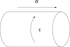
Figure 3: Left: the cylinder amplitude in string theory can be viewed either as a trace over the open string Hilbert space (quantizing along $\tau$) channel) or as an inner product between two wave functions in the closed string Hilbert space (quantizing along $\sigma$). Right: The global geometry of Lorentzian $AdS_{2}$ has the topology of a strip; its Euclidean continuation at finite temperature becomes a cylinder. $\tau$ and $t$ are the global and Poincaré time, respectively.

has two distinct conformal boundaries at $\sigma=0,\pi$, respectively; its Euclidean sections at finite temperature have the topology of a cylinder (see Figure 3).

Exercise 19

Check that the metric (7.6) is equivalent to (2.13) upon changing coordinates $\tau=\arctan(z+t)-\arctan(z-t)\ ,\quad\sigma=\arctan(z+t)+\arctan(z-t)$ . Map out the portion of the global geometry covered by the Poincaré coordinates $z,t$.

With this in mind, it is tempting to view (7.5) as an analogue of open/closed duality for conformal field theory on the cylinder,

$$\mbox{Tr}~{}e^{-\pi tH_{\rm open}}=\langle B^{\prime}|e^{-\frac{\pi}{t}H_{\rm closed}}|B\rangle$$ (7.7)

where $|B\rangle$ and $|B^{\prime}\rangle$ are closed string boundary states. The right-hand side of (7.5), analogue of the closed string channel, is identified with the partition function of quantum gravity on $AdS_{2}\times S^{2}$ in radial quantization along the space-like coordinate $\sigma$, with boundary conditions at $\sigma=0,\pi$ specified by the “boundary states” $\Psi^{\pm}_{p,q}$, while the left-hand side, analogue of the open string channel, is recognized as a trace of the identity operator in a sector of the Hilbert space for quantization along the global time coordinate $\tau$, with fixed charges $p^{I},q_{I}$ (the absence of an analogue of the Hamiltonians $H_{\rm open}$ and $H_{\rm closed}$ can be traced to diffeomorphism invariance, which requires physical states to be solutions of the Wheeler-De Witt equation $H|\psi\rangle=0$). It should be stressed that the Hilbert spaces for time-like and radial quantization are distinct, just like the open string and closed string Hilbert spaces are different.

For this interpretation to make sense, it should of course be possible to view $\Psi_{\rm top}$ as a state in the Hilbert space for radial quantization. This is, at least superficially, consistent with the wave function interpretation of $\Psi_{\rm top}$ discussed in Section 4.4, and would in fact provide a nice physical interpretation of this otherwise mysterious quantum mechanical behavior. Moreover, the functional dimension, $n_{V}+1$, of the Hilbert space hosting $\Psi_{\rm top}$, is roughly in accordance with the number of complex scalars $z^{i}$ varying radially in the black hole geometry. This leads one to expect that $\Psi_{\rm top}$ may provide a radial wave function for the vector-multiplet scalars, in a truncated Hilbert space where only static, spherically symmetric BPS configurations are kept. Such a “mini-superspace” truncation is usually hard to justify, but may hopefully be suitable for the purpose of computing indexed degeneracies of BPS black holes, in the same way as the Ramond-Ramond ground states in the closed string channel control the growth of the index in the open string Ramond sector.

This brings us to the problems of (i) quantizing the attractor flow (3.27),(3.28), (ii) showing that the resulting Hilbert space is the correct habitat for $\Psi_{\rm top}$, and (iii) finding a physical principle that selects $\Psi_{\rm top}$ among the continuum of states in that BPS Hilbert space. Answering these questions will be the subject of the rest of this chapter. Before doing so, several general remarks are in order:

• The idea of radial quantization of static black holes has a long history in the canonical gravity literature, e.g. [133, 134, 135, 136, 137, 138]. The main new ingredients here are supersymmetry, which may provide a better justification for the mini-superspace approximation, and holography, which offers the possibility to reconstruct the spectrum of the global time Hamiltonian from the overlap of two radial wave functions. The quantization of BPS configurations has been considered recently in various set-ups and found to agree with gauge theory computations [139, 140, 141, 142, 143, 144].

• The “channel duality” argument is in line with the usual AdS/CFT philosophy that the black hole micro-states should be described by “gauge theoretical” degrees of freedom living on the boundary of $AdS_{2}$. Contrary to higher dimensional AdS spaces, the conformal quantum mechanics describing $AdS_{2}$ is still largely mysterious, and the above approach is a possible indirect route towards determining its spectrum.

• One usually assumes that black hole micro-states can be described only in terms of the near horizon geometry. The above proposal to quantize the whole attractor flow seems to be at odds with this idea. A possible way out is that the topological wave function be a fixed point of the quantum attractor flow. In the sequel, we will study the full quantum attractor flow, from asymptotic infinity to the horizon, as a function of the Poincaré radial coordinate $r$ (rather than the “global radial coordinate $\sigma$”, which is well defined only near the horizon).

• The analogy between global $AdS_{2}$ and open strings explained below Eq. (7.7) can be pushed quite a bit further: due to pair production of charged particles, a black hole may fragment in different throats, analogous to the joining and splitting interactions of open strings [145] (see [146] for a perturbative approach to this problem). The study of exponentially suppressed corrections to the partition function in certain non-compact Calabi-Yau threefolds suggests that the attractor flow should be “second quantized” to allow for this possibility [112]. Note that the process whereby two ends of an open string join to form a closed string does not seem to have a black hole analogue.

• Finally, let us mention that further interest for the quantization of attractor flows stems from the relation between black hole attractor equations and the equations that determine supersymmetric vacua in flux compactifications (see e.g. [26] for a recent discussion). Upon double analytic continuation, one may hope to relate the black hole wave function to the wave function of the Universe, and address vacuum selection in the Landscape [7]. There are however many difficulties with this idea that we shall not discuss here. At any rate, it will be clear that our discussion of radial quantization bears many similarities with “mini-superspace” approaches to quantum cosmology.

7.2 Attractor Flows and Geodesic Motion

The most convenient route to quantize the attractor flow, or more generally perform the radial quantization of stationary, spherically symmetric black holes, is to use the equivalence between the equations governing the radial evolution of the fields in four dimensions, and the geodesic motion of a fiducial particle on an appropriate pseudo-Riemannian manifold [147]. This equivalence holds irrespective of supersymmetry, so we consider the general two-derivative action for four-dimensional gravity coupled to scalar fields $z^{i}$ and gauge fields $A_{4}^{I}$,

$$S_{4}=\frac{1}{2}\int\left[\sqrt{-\gamma}\ R[\gamma]\ d^{4}x+g_{ij}\ dz^{i}\wedge{}\star dz^{j}-F^{I}\wedge\Big{(}t_{IJ}{}\star F^{J}+\theta_{IJ}\wedge F^{J}\Big{)}\right].$$ (7.8)

Here, $\gamma$ denotes the four-dimensional metric, $g_{ij}$ the metric on the moduli space ${\cal M}_{4}$ where the (real) scalars $z^{i}$ take their values, $F^{I}=dA_{4}^{I}$ and the (positive definite) gauge couplings $t_{IJ}$ and angles $\theta_{IJ}$ are in general functions of $z^{i}$. In (7.8), we have dropped the contribution of the fermionic fields, but we shall reinstate them in Section 7.3 below when we return to a supersymmetric setting. Moreover, since the pseudo-Riemannian manifold already arises under the sole assumption of stationarity, we begin by relaxing the assumption of spherical symmetry.

7.2.1 Stationary solutions and $KK^{*}$ reduction

A general ansatz for stationary metrics and gauge fields is

$$\gamma_{\mu\nu}dx^{\mu}dx^{\nu}=-e^{2U}(dt+\omega)^{2}+e^{-2U}\gamma_{{\rm i}{\rm j}}dx^{\rm i}dx^{\rm j}\ ,\quad A_{4}^{I}=\zeta^{I}dt+A^{I}_{3}\ .$$ (7.9)

where the three-dimensional metric $\gamma_{{\rm i}{\rm j}}$, one-forms $A^{I}_{3},\omega$ and scalar $U,\zeta^{I},z^{i}$, are general functions of the coordinates $x^{\rm i}$ on the three-dimensional spatial slice. Since all these fields are independent of time, one may reduce the four-dimensional action (7.8) along the time direction and obtain a field theory in three Euclidean dimensions. This process is analogous to the usual Kaluza-Klein reduction, except for the time-like signature of the Killing vector $\partial_{t}$, which leads to unusual sign changes in the three-dimensional action.

Just as in usual Kaluza-Klein reduction, the one-forms $A^{I}_{3}$ and $\omega$ can be dualized into axionic scalars $\tilde{\zeta}_{I},\sigma$, using Hodge duality between one-forms and pseudo-scalars in three dimensions. Thus, the four-dimensional theory reduces to a gravity-coupled non-linear sigma model

$$S_{3}=\frac{1}{2}\int\ \left(\sqrt{g_{3}}\ R[g_{3}]\ d^{3}x+g_{ab}\ d\phi^{a}\wedge\star d\phi^{b}\right)$$ (7.10)

whose target manifold ${\cal M}_{3}^{*}$ includes the four-dimensional scalar fields $z^{i}$ together with $U$, $\zeta^{I}$, $\tilde{\zeta}_{I},\sigma$. The metric $g_{ab}$ on ${\cal M}_{3}^{*}$ has indefinite signature, and can be obtained by analytic continuation $(\zeta^{I},\tilde{\zeta}_{I})\to i(\zeta^{I},\tilde{\zeta}_{I})$ [147, 148] from the (Riemannian) three-dimensional moduli space ${\cal M}_{3}$ arising in standard, spacelike, Kaluza-Klein reduction, (see e.g. [149])

$$\begin{split}ds^{2}_{{\cal M}_{3}^{*}}&=2\,dU^{2}+g_{ij}\,dz^{i}dz^{j}+\frac{1}{2}e^{-4U}\left(d\sigma+\zeta^{I}d\tilde{\zeta}_{I}-\tilde{\zeta}_{I}d\zeta^{I}\right)^{2}\\ &-e^{-2U}\left[t_{IJ}\,d\zeta^{I}d\zeta^{J}+t^{IJ}\left(d\tilde{\zeta}_{I}+\theta_{IK}d\zeta^{K}\right)\left(d\tilde{\zeta}_{J}+\theta_{JL}d\zeta^{L}\right)\right]\end{split}$$ (7.11)

where $t^{IJ}\equiv[t^{-1}]^{IJ}$. Importantly, ${\cal M}_{3}^{*}$ always possesses (at least) $2n+2$ isometries corresponding to the gauge symmetries of $A^{I},\tilde{A}_{I},\omega$, as well as rescalings of time $t$. The Killing vector fields generating these isometries read

$$p^{I}=\partial_{\tilde{\zeta}_{I}}-\zeta^{I}\partial_{\sigma}\ ,\quad q_{I}=-\partial_{\zeta^{I}}-\tilde{\zeta}_{I}\partial_{\sigma}\ ,\quad k=\partial_{\sigma}\ ,$$ (7.12a)

$$M=-\left(\partial_{U}+\zeta^{I}\partial_{\zeta^{I}}+\tilde{\zeta}^{I}\partial_{\tilde{\zeta}^{I}}+2\sigma\partial_{\sigma}\right)$$ (7.12b)

and satisfy the Lie-bracket algebra

$$[p^{I},q_{J}]=-2\delta^{I}_{J}\ k$$ (7.13a)

$$[M,p^{I}]=p^{I}\ ,\quad\ [M,q_{I}]=q_{I}\ ,\quad[M,k]=2k$$ (7.13b)

In general, stationary solutions in four dimensions are therefore given by harmonic maps from the three-dimensional slice, with metric $\gamma_{{\rm i}{\rm j}}$, to the three-dimensional moduli space ${\cal M}_{3}^{*}$, such that Einstein’s equation in three-dimension is fulfilled,

$$R_{{\rm i}{\rm j}}[\gamma]=g_{ab}\left(\partial_{\rm i}\phi^{a}\partial_{\rm j}\,\phi^{b}-\frac{1}{2}\partial_{\rm k}\phi^{a}\,\partial_{\rm l}\phi^{b}\,\gamma^{{\rm k}{\rm l}}\,\gamma_{{\rm i}{\rm j}}\right)$$ (7.14)

Moreover, the Killing vectors $p^{I},q_{I},k,M$ give rise to conserved currents, whose conserved charges will be identified with the overall electric and magnetic charges, NUT charge and ADM mass of the configuration.

7.2.2 Spherical symmetry and geodesic motion

Now, let us restrict to spherically symmetric, stationary solutions: the spatial slices can be parameterized as

$$\gamma_{{\rm i}{\rm j}}dx^{\rm i}dx^{\rm j}=N^{2}(\rho)\,d\rho^{2}+r^{2}(\rho)\,(d\theta^{2}+\sin^{2}\theta\,d\phi^{2})$$ (7.15)

while all scalars on ${\cal M}_{3}^{*}$ become functions of $\rho$ only. After dropping a total derivative term, the three-dimensional sigma-model action reduces to classical mechanics,

$$S_{1}=\int d\rho\left[\frac{N}{2}+\frac{1}{2N}\left(r^{{}^{\prime}2}-r^{2}\,g_{ab}\,\phi^{{}^{\prime}a}\,\phi^{{}^{\prime}b}\right)\right]$$ (7.16)

where the prime denotes a derivative with respect to $\rho$. This Lagrangian describes the free motion of a fiducial particle on a cone ${\cal C}=\mathbb{R}^{+}\times{\cal M}_{3}^{*}$ over the three-dimensional moduli space ${\cal M}_{3}$. The lapse $N$ is an auxiliary field; its equation of motion enforces the mass shell condition

$$r^{{}^{\prime}2}-r^{2}\ g_{ab}\ \phi^{{}^{\prime}a}\ \phi^{{}^{\prime}b}=N^{2}$$ (7.17)

or equivalently, the Wheeler-De Witt (or Hamiltonian) constraint

$$H_{\rm WDW}=(p_{r})^{2}-\frac{1}{r^{2}}g^{ab}p_{a}p_{b}-1\equiv 0$$ (7.18)

where $p_{r},p_{a}$ are the canonical momenta conjugate to $r,\phi^{a}$.

Solutions are thus massive geodesics on the cone, with fixed mass equal to 1. In particular, the phase space describing the set of stationary, spherically symmetric solutions of (7.8) is the cotangent bundle $T^{*}{\cal C}$ of the cone ${\cal C}$.

As is most easily seen in the gauge $N=r^{2}$, the motion separates into geodesic motion on the base of the cone ${\cal M}_{3}^{*}$, with affine parameter $\tau$ such that $d\tau=d\rho/r^{2}(\rho)$, and motion along the radial direction $r$,

$$(p_{r})^{2}-\frac{C^{2}}{r^{2}}-1\equiv 0\ ,\quad g^{ab}p_{a}p_{b}\equiv C^{2}$$ (7.19)

where $p_{r}=r^{\prime}=\dot{r}/r^{2}$ and $p_{i}=r^{2}\phi^{{}^{\prime}i}=\dot{\phi}^{i}$; here the dot denotes a derivative with respect to $\tau$. It is interesting to note that the radial motion is governed by the same Hamiltonian as in [152], and therefore exhibits one-dimensional conformal invariance. This is a consequence of the existence of the homothetic Killing vector $r\partial_{r}$ on the cone ${\cal C}$.

7.2.3 Extremality and light-like geodesics

The motion along $r$ is easily integrated to

$$r=\frac{C}{\sinh(C\tau)}\ ,\quad\rho=\frac{C}{\tanh C\tau}$$ (7.20)

Assuming that the sphere $S^{2}$ reaches a finite area $A$ at the horizon $\tau=\infty$, so that $e^{-2U}r^{2}\to A/(4\pi)$, one may rewrite the metric (7.9) as [27]

$$ds^{2}\sim\frac{C^{2}}{\sinh^{2}(C\tau)}\left(-\frac{4\pi}{A}(dt+\omega)^{2}+\frac{A}{4\pi}d\tau^{2}\right)+\frac{A}{4\pi}d^{2}\Omega$$ (7.21)

The horizon at $\tau=\infty$ is degenerate for $C^{2}=0$, and non-degenerate for $C^{2}>0$, corresponding to extremal and non-extremal black holes, respectively. We conclude that extremal black holes correspond to light-like geodesics on ${\cal M}_{3}^{*}$ (it is indeed fortunate that ${\cal M}_{3}^{*}$ is a pseudo-Riemannian manifold, so that light-like geodesics do exist).

Exercise 20

Show that the extremality parameter $C$ is related to the Bekenstein–Haw-king entropy and Hawking temperature by $C=2S_{BH}T_{H}$.

Setting $C=0$ in (7.19), we moreover see that $r=\rho=1/\tau$, and therefore that the spatial slices in the ansatz (7.9) are flat. We could therefore have set $N=1,r=1/\tau$ from the start, and obtained the action for geodesic motion on ${\cal M}_{3}$ in affine parameterization,

$$S_{1}^{\prime}=\int d\tau~{}\frac{1}{2}~{}g_{ab}~{}\dot{\phi}^{a}~{}\dot{\phi^{b}}$$ (7.22)

While one may dispose of the radial variable $r$ altogether, it is however advantageous to retain it for the purpose of defining observables such as the horizon area, $A_{H}=4\pi e^{-2U}r^{2}|_{U\to-\infty}$ and the ADM mass $M=r(e^{2U}-1)|_{U\to 0}$.

7.2.4 Conserved charges and black hole potential

As anticipated by the notation in (7.13a), the isometries of ${\cal M}_{3}$ imply conserved Noether charges,

$$q_{I}\ d\tau = -2e^{-2U}\left[t_{IJ}d\zeta^{J}+\theta_{IJ}t^{JL}\left(d\tilde{\zeta}_{L}+\theta_{LM}d\zeta^{M}\right)\right]+2\,k\tilde{\zeta}_{I}$$

$$p^{I}\ d\tau = -2e^{-2U}t^{IL}\left(d\tilde{\zeta}_{L}+\theta_{LM}d\zeta^{M}\right)-2\,k\zeta^{I}$$ (7.23)

$$k\ d\tau = e^{-4U}\left(d\sigma+\zeta^{I}d\tilde{\zeta}_{I}-\tilde{\zeta}^{I}d\zeta_{I}\right)$$

(as well as $M$, whose precise form we will not need) identified as the electric, magnetic and NUT charges $p^{I},q_{I},k$. Their algebra under Poisson bracket is the same as algebra of the Killing vectors under Lie bracket,

$$\{p^{I},q_{J}\}_{\rm PB}=-2\delta^{I}_{J}k\ ,\quad\{M,p^{I}\}_{\rm PB}=p^{I}\ ,\quad\ \{M,q_{I}\}_{\rm PB}=q_{I}\ ,\quad\{M,k\}_{\rm PB}=2k$$ (7.24)

In particular, the electric and magnetic charges satisfy an Heisenberg algebra, the center of which is the NUT charge $k$. The latter is related to the off-diagonal term in the metric (7.9) via $\omega=k\cos\theta\ d\phi$. When $k\neq 0$, the metric

$$ds_{4}^{2}=-e^{2U}(dt+k\cos\theta\,d\phi)^{2}+e^{-2U}\left(d\rho^{2}+r^{2}(\rho)[d\theta^{2}+\sin^{2}\theta\,d\phi^{2}]\right)$$ (7.25)

has closed timelike curves along the compact $\phi$ coordinates near $\theta=0$, all the way from infinity to the horizon. Bona fide 4D black holes have $k=0$, which corresponds to a “classical” limit of the Heisenberg algebra (7.24).

Using the conserved charges (7.2.4), one may express the Hamiltonian for affinely parameterized geodesic motion on ${\cal M}_{3}^{*}$ as

$$H\equiv p^{a}g_{ab}p^{b}=\frac{1}{2}\left[p_{U}^{2}+\frac{1}{4}p_{z^{i}}g^{ij}p_{z^{j}}-e^{2U}V_{BH}+k^{2}e^{4U}\right]$$ (7.26)

where $p_{U},p_{z^{i}}$ are the momenta canonically conjugate to $U,z^{i}$,

$$V_{BH}(p,q,z)=-\frac{1}{2}(\hat{q}_{I}-\theta_{IJ}\hat{p}^{J})t^{IK}(\hat{q}_{K}-\theta_{KL}\hat{p}^{L})-\frac{1}{2}\hat{p}^{I}t_{IJ}\hat{p}^{J}$$ (7.27)

and

$$\hat{p}^{I}=p^{I}+2k\zeta^{I}\ ,\quad\hat{q}_{I}=q_{I}-2k\zeta^{I}\ ,\quad$$ (7.28)

For $k=0$, the motion along $\zeta^{I},\tilde{\zeta}_{I},\sigma$ separates from that along $U,z^{i}$, effectively producing a potential for these variables. Following [55], we refer to $V_{BH}$ as the “black hole potential”, but it should be kept in mind that it contributes negatively to the actual potential $V=-e^{2U}V_{BH}+k^{2}e^{4U}$ governing the Hamiltonian motion. In Figure 4, we plot the potential $V$ for $\mathcal{N}=2$ supergravity with one minimally coupled vector multiplet.

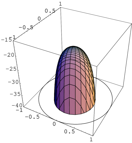
Figure 4: Potential governing the radial evolution of the complex scalar in the same model as in Figure 2 and same charges, at $U=0$. The potential has a global maximum at $z_{*}=X^{1}/X^{0}=(1-3i)/10$.

7.2.5 The Universal Sector

As an illustration, and a useful warm-up for the symmetric case discussed in Section 7.5 below, it is instructive to work out the dynamics in the “universal sector”, which encodes the scale $U$, the graviphoton electric and magnetic charges, and the NUT charge $k$. The resulting pseudo-quaternionic-Kähler manifold is the symmetric space ${\cal M}_{3}^{*}=SU(2,1)/Sl(2)\times U(1)$, an analytic continuation of the quaternionic-Kähler space ${\cal M}_{3}=SU(2,1)/SU(2)\times U(1)$, which describes the tree-level couplings of the universal hypermultiplet in 4 dimensions. It is obtained via c-map from a trivial moduli space $\mathcal{M}_{4}$ corresponding to the prepotential $F=-i(X^{0})^{2}/2$. The Hamiltonian (7.26) becomes

$$H=\frac{1}{8}(p_{U})^{2}-\frac{1}{4}e^{2U}\left[(p_{\tilde{\zeta}}-k\zeta)^{2}+(p_{\zeta}+k\tilde{\zeta})^{2}\right]+\frac{1}{2}e^{4U}k^{2}$$ (7.29)

The motion separates between the $(\tilde{\zeta},\zeta)$ plane and the $U$ direction, while the NUT potential $\sigma$ can be eliminated in favor of its conjugate momentum $k=e^{-4U}(\dot{\sigma}+\zeta\dot{\tilde{\zeta}}-\tilde{\zeta}\dot{\zeta})$. The motion in the $(\tilde{\zeta},\zeta)$ plane is that of a charged particle in a constant magnetic field. The electric, magnetic charges and the angular momentum $J$ in the plane (not to be confused with that of the black hole, which vanishes by spherical symmetry)

$$p=p_{\tilde{\zeta}}+\zeta k\ ,\quad q=p_{\zeta}-\tilde{\zeta}k\ ,\quad J=\zeta p_{\tilde{\zeta}}-\tilde{\zeta}p_{\zeta}$$ (7.30)

satisfy the usual algebra of the Landau problem,

$$\{p,q\}_{\rm PB}=2k\ \quad,\{[J,p\}_{\rm PB}=q\ ,\quad\{J,q\}_{\rm PB}=-p$$ (7.31)

where $p$ and $q$ are the “magnetic translations”. The motion in the $U$ direction is governed effectively by

$$H=\frac{1}{8}(p_{U})^{2}+\frac{1}{2}e^{4U}k^{2}-\frac{1}{4}e^{2U}\left[p^{2}+q^{2}-4kJ\right]=C^{2}$$ (7.32)

The potential is depicted on Figure 5 (left). At spatial infinity ($\tau=0$), one may impose the initial conditions $U=\zeta=\tilde{\zeta}=a=0$. The momentum $p_{U}$ at infinity is proportional to the ADM mass, and $J$ vanishes, so the mass shell condition (7.29) becomes

$$M^{2}+2k^{2}-(p^{2}+q^{2})=C^{2}$$ (7.33)

Extremal black holes correspond to $C^{2}=0$; in this low dimensional example are automatically BPS, as we shall see in the next Section. Equation (7.33) is then the BPS mass condition, generalized to non-zero NUT charge. Note that for a given value of $p,q$, there is a maximal value of $k$ such that $M^{2}$ remains positive.

At the horizon $U\to-\infty$, $\tau\to\infty$, the last term in (7.29) is irrelevant, and one may integrate the equation of motion of $U$, and verify that the metric (7.9) becomes $AdS_{2}\times S^{2}$ with area

$$A=2\pi(p^{2}+q^{2})=2\pi\sqrt{(p^{2}+q^{2})^{2}}$$ (7.34)

in agreement with the Bekenstein-Hawking entropy of Reissner-Nordström black holes (2.15).

Figure 5: Left: Potential governing the motion along the $U$ variable in the universal sector. The horizon is reached at $U\to-\infty$. Right: Root diagram of the $SU(2,1)$ symmetries in the universal sector.

Since the universal sector is a symmetric space, there must exist 3 additional conserved charges, so that the total set of conserved charges can be arranged in an element $Q$ in the Lie algebra ${\mathfrak{g}}_{3}=su(2,1)$ (or rather, in its dual ${\mathfrak{g}}_{3}^{*}$),

$$Q=\begin{pmatrix}M+iJ/3&{E_{p}}-i{E_{q}},&i{E_{k}}\\ {E_{p^{\prime}}}+i{E_{q^{\prime}}}&-2iJ/3&-({E_{p}}+i{E_{q}})\\ -i{E_{k^{\prime}}}&-({E_{p^{\prime}}}-i{E_{q^{\prime}}})&-M+iJ/3\end{pmatrix}$$ (7.35)

where $M,E_{p}\equiv p^{0},E_{q}\equiv q_{0},E_{k}\equiv k$ have been given in (7.12a) and $J=\zeta\partial_{\tilde{\zeta}}-\tilde{\zeta}\partial_{\zeta}$. The remaining Killing vectors can be easily found [12],

$$E_{p^{\prime}} = -\tilde{\zeta}\partial_{U}-(\sigma+2\zeta\tilde{\zeta})\partial_{\zeta}+\left[e^{2U}+\frac{1}{2}(3\zeta^{2}-\tilde{\zeta}^{2})\right]\partial_{\tilde{\zeta}}+\left[\zeta\left(e^{2U}+\frac{1}{2}(\zeta^{2}+\tilde{\zeta}^{2})\right)-\sigma\tilde{\zeta}\right]\partial_{\sigma}$$

$$E_{q^{\prime}} = \zeta\partial_{U}-\left[e^{2U}+\frac{1}{2}(3\tilde{\zeta}^{2}-\zeta^{2})\right]\partial_{\zeta}-(\sigma-2\zeta\tilde{\zeta})\partial_{\tilde{\zeta}}+\left[\tilde{\zeta}\left(e^{2U}+\frac{1}{2}(\zeta^{2}+\tilde{\zeta}^{2})\right)+\sigma\zeta\right]\partial_{\sigma}$$

$$E_{k^{\prime}} = -\sigma\partial_{U}+\left[\left(e^{2U}+\frac{1}{2}(\zeta^{2}+\tilde{\zeta}^{2})\right)^{2}-\sigma^{2}\right]\partial_{\sigma}$$

$$-\left[\tilde{\zeta}\left(e^{2U}+\frac{1}{2}(\zeta^{2}+\tilde{\zeta}^{2})\right)+\sigma\zeta\right]\partial_{\zeta}+\left[\zeta\left(e^{2U}+\frac{1}{2}(\zeta^{2}+\tilde{\zeta}^{2})\right)-\sigma\tilde{\zeta}\right]\partial_{\tilde{\zeta}}$$

The physical origin of these extra symmetries are the Ehlers and Harrison transformations, well known to general relativists [153]. It is easy to check that these Killing vectors satisfy the Lie algebra of $SU(2,1)$, whose root diagram is depicted on Figure 5. The Casimir invariants of $Q$ can be easily computed:

$$\mbox{Tr}(Q^{2})=H\ ,\quad\det(Q)=0$$ (7.36)

The last condition ensures that the conserved quantities do not overdetermine the motion. The co-adjoint action $Q\to hQh^{-1}$ of $G_{3}$ on ${\mathfrak{g}}_{3}^{*}$ relates different trajectories with the same value of $H$. The phase space, at fixed value of $H$, is therefore a generic co-adjoint orbit of $G_{3}$, of dimension 6 (the symplectic quotient of the full 8-dimensional phase space by the Hamiltonian $H$). By the Kirillov-Kostant construction, it carries a canonical symplectic form such that the Noether charges represent the Lie algebra ${\mathfrak{g}}_{3}$.

As we have just seen, extremal solutions have $H=0$. The standard property of $3\times 3$ matrices

$$Q^{3}-\mbox{Tr}(Q)Q^{2}+\frac{1}{2}[\mbox{Tr}(Q^{2})-(\mbox{Tr}Q)^{2}]Q-\det(Q)=0$$ (7.37)

then implies that $Q^{3}=0$, as a matrix equation in the fundamental representation; more intrinsically, in terms of the adjoint representation, this is equivalent to

$$[Ad(Q)]^{5}=0$$ (7.38)

Thus, $Q$ is a nilpotent element of order 5 in ${\mathfrak{g}}_{3}^{*}$. This condition is invariant under the co-adjoint action of $G_{3}$. We conclude that the classical phase space of extremal configurations is a nilpotent coadjoint orbit of $G_{3}$. By the general “orbit philosophy” [154], the quantum Hilbert space then furnishes a “unipotent” representation of $G_{3}$, obtained by quantizing this nilpotent co-adjoint orbit. As we shall see in Section 7.5, this fact extends to the BPS Hilbert space in very special supergravities, where ${\cal M}_{3}^{*}$ is a symmetric space.

7.3 BPS black holes and BPS geodesics

Up till now, our discussion did not assume any supersymmetry. In general however, the KK^∗ reduction of the fermions gives extra fermionic contributions in (7.10), such that the resulting non-linear sigma model has the same amount of supersymmetry as its four-dimensional parent. Moreover, the spherical reduction of the fermions preserves half of the supersymmetries. This leads to the action for a supersymmetric spinning particle moving on $\mathcal{C}$, schematically

$$S_{1}=\int d\tau~{}\left[g_{ab}{\dot{\phi}}^{a}{\dot{\phi}}^{b}+g_{ab}\ \psi^{a}D_{\tau}\psi^{b}+R_{abcd}\psi^{a}\psi^{b}\psi^{c}\psi^{d}\right]$$ (7.39)

This Lagrangian is supersymmetric for any target space, but has $N$-fold extended supersymmetry when $\mathcal{C}$ admits $N-1$ complex structures $J^{(i)}$ ($i=1,\dots,N-1$). The supersymmetry variations of the fermions are then of the form

$$\delta_{\epsilon}\psi^{a}=\sum_{i=0}^{N-1}\epsilon^{(i)}J^{(i)a}_{b}\dot{\phi}^{b}+O(\psi^{2})$$ (7.40)

with $J^{(0)a}_{b}=\delta^{a}_{b}$ the identity operator. Moreover, the existence of a homothetic Killing vector $r\partial_{r}$ implies that the action $S_{1}$ should be superconformally invariant.

BPS solutions in four dimensions correspond to special trajectories on ${\cal M}_{3}^{*}$, for which there exist a non-zero $\epsilon^{(i)}$ such that the right-hand side of (7.40) vanishes. This puts a strong constraint on the momentum $p_{a}=g_{ab}\dot{\phi}^{b}$ of the fiducial particle, which defines a “BPS” subspace of the phase space $T^{*}(\mathcal{C})$. The symplectic structure on this BPS phase space can then be obtained using Dirac’s theory of Hamiltonian constraints. Due to the existential quantifier $\exists\epsilon^{(i)}\neq 0$, it is sometimes convenient to extend the phase space by including the Killing spinor $\epsilon^{(i)}$, we shall see an example of this in Section 7.3.2. In theories with $N\geq 2$ supersymmetry in 4 dimensions, black holes may preserve different fractions of supersymmetry, associated to different orbits of the momentum $p$ under the holonomy group of $\mathcal{C}$. Correspondingly there will be different BPS phase spaces, nested into each other.

7.3.1 Attractor Flow and BPS Geodesic Flow in ${\cal N}=2$ SUGRA

After this deliberately schematic discussion, we now specialize to ${\cal N}=2$ supergravity, and show that the attractor flow (3.27),(3.28) is indeed equivalent to BPS geodesic flow on the three-dimensional moduli space ${\cal M}_{3}^{*}$.

As explained in Section 3, ${\cal N}=2$ supersymmetry determines the metric on $\mathcal{M}_{4}$ (now denoted $g_{i\bar{\jmath}}$, to take into account the complex nature of the vector multiplet moduli) and gauge couplings $\theta_{IJ}-it_{IJ}\equiv{\cal N}_{IJ}$ in terms of a prepotential $F(X)$ via (3.3),(3.11). The scalar manifold ${\cal M}_{3}$ obtained by Kaluza-Klein reduction to three dimensions is now a quaternionic-Kähler space, usually referred to as the “c-map” of the special Kähler manifold ${\cal M}_{4}$ [155, 149]. The analytically continued ${\cal M}_{3}^{*}$, with metric (7.11) is a pseudo-quaternionic-Kähler space, which we shall refer to as the “c^∗-map” of ${\cal M}_{4}$. While ${\cal M}_{3}$ has a Riemannian metric with special holonomy $USp(2)\times USp(2n_{V}+2)$, ${\cal M}_{3}^{*}$ has a split signature metric with special holonomy $Sp(2)\times Sp(2n_{V}+2)$. For convenience, we will work with the Riemannian space ${\cal M}_{3}$ and perform the analytic continuation at the end.

In order to determine the couplings of the corresponding fermions, one should in principle reduce the four-dimensional fermions along the time direction, then further on the spherically symmetric ansatz (7.15). For our present purposes however, it is sufficient to recall that the quaternionic-Kähler space ${\cal M}_{3}$ equivalently arises as the target space of a $N=2$ supersymmetric sigma model in 3+1 dimensions, coupled to gravity [156]. Upon reducing the action and supersymmetry transformations of [156] along three flat spatial directions, one obtains a $N=4$ supersymmetric sigma model in 0+1 dimensions, which must be identical to the result of the spherical reduction. The supersymmetry variations are then simply

$$\delta_{\epsilon}\phi^{a}=O(\psi)\ ,\quad\delta_{\epsilon}\psi^{AA^{\prime}}=V^{AB^{\prime}}_{a}\dot{\phi}^{a}\epsilon^{A^{\prime}}_{B^{\prime}}+O(\psi^{2})$$ (7.41)

Here, $V^{AA^{\prime}}$ ($A=1,..,2n_{V}+2$ and $A^{\prime}=1,2$) is the “quaternionic viel-bein” afforded by the decomposition

$$T_{\mathbb{C}}{\cal M}_{3}=E\otimes H$$ (7.42)

of the complexified tangent bundle of  ${\cal M}_{3}$, where $E$ and $H$ are complex vector bundles of respective dimensions $2n_{V}+2$ and $2$. Similarly, the Levi-Civita connection decomposes into its $USp(2)$ and $USp(2n_{V}+2)$ parts $p$ and $q$,

$$\Omega_{AA^{\prime}}^{BB^{\prime}}=p^{A^{\prime}}_{B^{\prime}}\epsilon_{A}^{B}+q^{A}_{B}\epsilon_{A^{\prime}}^{B^{\prime}}$$ (7.43)

where $\epsilon_{A^{\prime}B^{\prime}}$ and $\epsilon_{AB}$ are the antisymmetric tensors invariant under $USp(2)$ and $USp(2n)$. The viel-bein $V$ controls both the metric and the three almost complex structures on the quaternionic-Kähler space,

$$ds^{2}=\epsilon_{A^{\prime}B^{\prime}}\ \epsilon_{AB}\ V^{AA^{\prime}}\otimes V^{BB^{\prime}}\ ,\quad\Omega^{i}=\epsilon_{A^{\prime}B^{\prime}}\ (\sigma^{i})^{B^{\prime}}_{C^{\prime}}\ \epsilon_{AB}\ V^{AA^{\prime}}\wedge V^{BC^{\prime}}$$ (7.44)

(where $\sigma^{i}$, $i=1,2,3$ are the Pauli matrices) and is covariantly constant with respect to the connection (7.43).

From (7.41), it is apparent that supersymmetric solutions are obtained when $V^{AA^{\prime}}$ has a zero right-eigenvector,

SUSY $$\Leftrightarrow \quad\exists\epsilon_{A^{\prime}}\neq 0\ /\ V^{AA^{\prime}}\epsilon_{A^{\prime}}=0$$ (7.45a)

$$\Leftrightarrow \quad\forall\,A,B\ ,\quad\epsilon_{A^{\prime}B^{\prime}}\,V^{AA^{\prime}}\,V^{BB^{\prime}}=0$$ (7.45b)

For fixed $\epsilon^{A^{\prime}}$, these are $2n_{V}+2$ conditions on the velocity vector $\dot{\phi}^{a}$ at any point along the geodesic, removing half of the degrees of freedom from the generic trajectories. In particular, the conditions (7.45b) imply that

$$\epsilon_{AB}\epsilon_{A^{\prime}B^{\prime}}V^{AA^{\prime}}V^{BB^{\prime}}=0=H\ ,$$ (7.46)

and therefore that a BPS solution is automatically extremal. For the universal sector discussed in Section 7.2.5, where $n_{V}=0$, this is actually a necessary and sufficient condition for supersymmetry.

For the case of the $c$-map ${\cal M}_{3}$, the quaternionic viel-bein was computed explicitly in [149]. After analytic continuation, one obtains

$$V^{AA^{\prime}}=\begin{pmatrix}iu&v\\ e^{a}&iE^{a}\\ -i\bar{E}^{\bar{a}}&\bar{e}^{\bar{a}}\\ -\bar{v}&i\bar{u}\end{pmatrix}$$ (7.47)

where $e^{a}=e^{a}_{i}dz^{i}$ is a viel-bein of the special Kähler manifold, $e^{a}_{i}\bar{e}_{\bar{a}\overline{\jmath}}\delta_{a\bar{a}}=g_{i\overline{\jmath}}$, and

$$u = e^{\mathcal{K}/2-U}X^{I}\left(d\tilde{\zeta}_{I}+{\cal N}_{IJ}d\zeta^{J}\right)$$ (7.48)

$$v = -dU+\frac{i}{2}e^{-2U}\left(d\sigma+\zeta^{I}d\tilde{\zeta}_{I}-\tilde{\zeta}^{I}d\zeta_{I}\right)$$ (7.49)

$$E^{a} = e^{-U}e^{a}_{i}g^{i\overline{\jmath}}\bar{f}_{\overline{\jmath}}^{I}\left(d\tilde{\zeta}_{I}+{\cal N}_{IJ}d\zeta^{J}\right)$$ (7.50)

Expressing $d\zeta^{I},d\tilde{\zeta}_{I},d\sigma$ in terms of the conserved charges (7.23), the entries in the quaternionic viel-bein may be rewritten as

$$u = -\frac{i}{2}e^{\mathcal{K}/2+U}X^{I}\left[q_{I}-2k\tilde{\zeta}_{I}-{\cal N}_{IJ}(p^{J}+2k\zeta^{J})\right]d\tau\ ,\quad$$ (7.51)

$$v = -dU+\frac{i}{2}e^{2U}k\ d\tau$$ (7.52)

$$e^{a} = e^{a}_{i}\ dz^{i}\ ,\quad$$ (7.53)

$$E^{a} = -\frac{i}{2}e^{U}e^{ai}g^{i\overline{\jmath}}\bar{f}_{\overline{\jmath}}^{I}\left[q_{I}-2k\tilde{\zeta}_{I}-{\cal N}_{IJ}(p^{J}+2k\zeta^{J})\right]d\tau$$ (7.54)

Now, return to the supersymmetry variation of the fermions (7.41): the existence of $\epsilon_{A^{\prime}}^{B^{\prime}}$ such that $\delta\psi^{AA^{\prime}}$ vanishes implies that the first column of $V$ has to be proportional to the second, hence

$$-\frac{dU}{d\tau}+\frac{i}{2}e^{2U}k = -\frac{i}{2}\ e^{i\theta}\ e^{\mathcal{K}/2+U}\ X^{I}\left(q_{I}-k\tilde{\zeta}_{I}-{\cal N}_{IJ}(p^{J}+k\zeta^{J})\right)$$ (7.55)

$$\frac{dz^{i}}{d\tau} = -\frac{i}{2}\ e^{i\theta}\ e^{U}\ g^{i\overline{\jmath}}\bar{f}_{\overline{\jmath}}^{I}\left(q_{I}-k\tilde{\zeta}_{I}-{\cal N}_{IJ}(p^{J}+k\zeta^{J})\right)$$ (7.56)

where the phase $\theta$ is determined by requiring that $U$ stays real. These equations may be rewritten as

$$-\frac{dU}{d\tau}+\frac{i}{2}e^{2U}k=-\frac{i}{2}e^{i\theta}e^{U}Z\ ,\quad\frac{dz^{i}}{d\tau}=-ie^{i\theta}\frac{|Z|}{Z}e^{U}g^{i\overline{\jmath}}\partial_{\overline{\jmath}}|Z|$$ (7.57)

where $\hat{Z}$ is the “generalized central charge”

$$\hat{Z}(p,q,k)=e^{\mathcal{K}/2}\left[\hat{q}_{I}X^{I}-\hat{p}^{I}F_{I}\right]$$ (7.58)

and $\hat{p}^{I},\hat{q}_{I}$ have been defined in (7.28). For vanishing NUT charge, we recognize the attractor flow equations (3.27),(3.28). The equivalence between the attractor flow equations on ${\cal M}_{4}$ and supersymmetric geodesic motion on ${\cal M}_{3}$ was in fact observed long ago in [157], and is a consequence of T-duality between black holes and instantons, after compactifying to three dimensions [158, 159].

This concludes our proof that BPS geodesics, characterized by the BPS constraints (7.45), indeed describe stationary, spherically symmetric BPS black holes.

7.3.2 Swann space and twistor space

While the analysis in the previous section identified the BPS subspace of the phase space $T^{*}\mathcal{M}_{3}^{*}$ (namely, the solution to the quadratic constraints (7.45b)), the non-linearity of the BPS constraints makes it difficult to obtain its precise symplectic structure. We now show that, by lifting the geodesic motion on the quaternionic-Kähler $\mathcal{M}_{3}^{*}$ to a higher-dimensional space, namely the Swann space $\mathcal{S}$, it is possible to linearize these constraints.

The Swann space is a standard construction, which relates quaternionic-Kähler geometry in dimension $4n_{V}+4$ to hyperkähler geometry in $4n_{V}+8$ dimensions [160]. Namely, let $\pi^{A^{\prime}}$ ($A^{\prime}=1,2$) be complex coordinates in the vector bundle $H$ over ${\cal M}_{3}$, and $\mathcal{S}$ be the total space of this bundle. $\mathcal{S}$ admits a hyperkähler metric

$$ds^{2}_{\mathcal{S}}=|D\pi|^{2}+R^{2}\,ds^{2}_{{\cal M}_{3}}\,.$$ (7.59)

where

$$D\pi^{A^{\prime}}=d\pi^{A^{\prime}}+p^{A^{\prime}}_{B^{\prime}}\pi^{B^{\prime}}\ ,\quad R^{2}\equiv|\pi|^{2}=|\pi^{1}|^{2}+|\pi^{2}|^{2}$$ (7.60)

In fact, $R^{2}$ is the hyperkähler potential of (7.59), i.e. a Kähler potential for all complex structures. Being hyperkähler, $\mathcal{S}$ has holonomy $USp(2n_{V}+4)$; the corresponding covariantly constant vielbein ${\cal V}^{\aleph}$ (where $\aleph\in\{A,A^{\prime}\}$ runs over two more indices than $A$) can be simply obtained from the quaternionic vielbein $V^{AA^{\prime}}$ on the base $\mathcal{M}_{3}$ via

$${\cal V}^{A}=V^{AA^{\prime}}\pi_{A^{\prime}}\ ,\quad{\cal V}^{A^{\prime}}=D\pi^{A^{\prime}}$$ (7.61)

The viel-bein ${\cal V}^{\aleph}$ gives a set of $(1,0)$-forms on $\mathcal{S}$ (for a particular complex structure), which together with $\bar{\cal V}$, span the cotangent space of $\mathcal{S}$. The fermionic variations in the corresponding sigma model split into

$$\delta_{\epsilon}\psi^{\aleph}=\mathcal{V}^{\aleph}\epsilon+\dots\ ,\quad\delta_{\bar{\epsilon}}\bar{\psi}^{\bar{\aleph}}=\bar{\mathcal{V}}^{\aleph}\bar{\epsilon}+\dots$$ (7.62)

Moreover, the metric (7.59) has a manifest $SU(2)$ isometry, and homothetic Killing vector $R\partial_{R}=\pi^{A^{\prime}}\partial_{\pi^{A^{\prime}}}+\bar{\pi}^{A^{\prime}}\partial_{\bar{\pi}^{A^{\prime}}}$. Geodesic motion on $\mathcal{S}$ is therefore equivalent to geodesic motion on the base $\mathcal{M}_{3}$, provided one restricts to trajectories with zero angular momentum under the $SU(2)$ action (and disregard the motion along the radial direction $R^{2}=|\pi|^{2})$. By suitable $SU(2)$ rotation, BPS geodesics on $\mathcal{S}$ can be chosen to be annihilated by $\delta_{\epsilon}$, and so correspond to

$$\forall\,\aleph\ ,\qquad\mathcal{V}^{\aleph}=0$$ (7.63)

Using (7.61), this entails

$$V^{AA^{\prime}}\pi_{A^{\prime}}=0\ ,\quad D\pi^{A^{\prime}}=0$$ (7.64)

The first condition reproduces the BPS condition (7.45a) on $\mathcal{M}_{3}$ upon identifying $\pi^{A^{\prime}}$ with the Killing spinor $\epsilon_{A^{\prime}}$, while the second can be shown to follow from the Killing spinor conditions in four dimensions, consistently with this identification. The condition (7.63) shows that BPS trajectories are such that the momentum vector is anti-holomorphic at every point. These BPS constraints are clearly first class, and therefore the extended BPS phase space is the Swann space $\mathcal{S}$ itself, equipped with its Kähler form.

While the Swann space has a clear physical motivation, the fiber being identified with the Killing spinor, the fact that one must restrict to $\mathbb{R}^{\times}\times SU(2)$ invariant trajectories means that it is somewhat too large. In fact, one may perform a symplectic reduction – more precisely, a Kähler quotient – with respect to $U(1)\subset SU(2)$ while keeping most of the pleasant properties of the Swann space. The result, known as the twistor space $\mathcal{Z}$, retains one of the three complex structures of $\mathcal{S}$, which is sufficient for exposing half of the $\mathcal{N}=4$ supersymmetries of (7.39). To exhibit the structure of $\mathcal{Z}$, it is useful to choose the following coordinates on the unit sphere in $\mathbb{R}^{4}$,

$$e^{i\varphi}=\sqrt{\pi^{2}/\bar{\pi}^{2}}\ ,\quad z={\pi^{1}}/{\pi^{2}}\,.$$ (7.65)

where $\varphi$ is the angular coordinate for the Hopf fibration $U(1)\to S^{3}\to S^{2}$ and $z$ is a stereographic coordinate on $S^{2}=\mathbb{C}\mathbb{P}^{1}$. In these coordinates, the metric (7.59) rewrites as

$$ds^{2}_{\mathcal{S}}=dR^{2}+R^{2}\left[D\phi^{2}+\frac{DzD\bar{z}}{(1+z\bar{z})^{2}}+ds^{2}_{\mathcal{M}_{3}}\right]$$ (7.66)

where

$$Dz \equiv dz-\frac{1}{2}(p_{1}+ip_{2})-2p_{3}z-\frac{1}{2}(p_{1}-ip_{2})z^{2}\ ,$$ (7.67)

$$D\phi \equiv d\phi+\frac{i}{2(1+z\bar{z})}\left(z[d\bar{z}-(p_{1}+ip_{2})]-\bar{z}[dz-(p_{1}-ip_{2})]-2ip_{3}(1-\bar{z}z)\right)$$

and $p_{i}=\sigma_{(i)}^{A^{\prime}B^{\prime}}p_{(A^{\prime}B^{\prime})}$. The connection term in $Dz$ is sometimes known as the projectivized $USp(2)$ connection. The twistor space $\mathcal{Z}$ is the Kähler quotient of $\mathcal{S}$ by $U(1)$ rotations along $\phi$ [161]; its metric is therefore given by the last two terms in (7.66)

$$ds^{2}_{\mathcal{Z}}=\frac{|Dz|^{2}}{(1+\bar{z}z)^{2}}+ds^{2}_{\mathcal{M}_{3}}\,.$$ (7.68)

The space $\mathcal{Z}$ is itself an $S^{2}$ bundle over ${\cal M}_{3}$ and carries a canonical complex structure, which is an integrable linear combination of the triplet of almost complex structures on $\mathcal{M}_{3}$. It will also be important that $\mathcal{Z}$ carries a holomorphic contact structure $X$ (proportional to the one-form $Dz$), inherited from the holomorphic symplectic structure on the hyperkähler cone $\mathcal{S}$.

For later purposes, it will be useful to have an explicit set of $2n_{V}+3$ complex coordinates $(\xi^{I},\tilde{\xi}_{I},\alpha)$ on the twistor space $\mathcal{Z}$, adapted to the Heisenberg symmetries, i.e. such that the Killing vectors $p^{I},q_{I},k$ in (7.12a) take the standard form

$$p^{I}=\partial_{\tilde{\xi}_{I}}-\xi^{I}\partial_{\alpha}+\mbox{c.c.}\ ,\quad q_{I}=-\partial_{\xi^{I}}-\tilde{\xi}_{I}\partial_{\alpha}+\mbox{c.c.}\ ,\quad k=\partial_{\alpha}+\mbox{c.c.}$$ (7.69)

while the holomorphic contact structure takes the canonical, Darboux form,

$$X=d\alpha+\tilde{\xi}_{I}d\xi^{I}-\xi_{I}d\tilde{\xi}^{I}$$ (7.70)

Such a coordinate system has been constructed recently in [11], from which we collect the relevant formulae. The complex coordinates $(\xi^{I},\tilde{\xi}_{I},\alpha)$ are related to the coordinates $U,z^{i},\bar{z}^{\bar{i}},\zeta^{I},\tilde{\zeta}_{I},\sigma$ on the quaternionic-Kähler base, as well as the fiber coordinate $z\in{\mathbb{C}P}_{1}$, via the “twistor map”

$$\xi^{I} = \zeta^{I}+2i\ e^{U+{\cal K}(X,\bar{X})/2}\left(z\bar{X}^{I}+z^{-1}X^{I}\right)$$ (7.71a)

$$\tilde{\xi}_{I} = \tilde{\zeta}_{I}+2i\ e^{U+{\cal K}(X,\bar{X})/2}\left(z\ \bar{F}_{I}+z^{-1}\ F_{I}\right)$$ (7.71b)

$$\alpha = \sigma+\zeta^{I}\tilde{\xi}_{I}-\tilde{\zeta}_{I}\xi^{I}$$ (7.71c)

These formulae were derived in [11] by using the projective superspace description of the $c$-map found in [162]. A key feature of these formulae is that, for a fixed point on the base, the complex coordinates $\xi^{I},\tilde{\xi}_{I},\alpha$ depend rationally on the fiber coordinate $\mathcal{Z}$; said differently, the fiber over any point on the base is rationally in $\mathcal{Z}$. This is a general property of twistor spaces, which allows for the existence of the Penrose transform relating holomorphic functions on $\mathcal{Z}$ to harmonic-type functions on $\mathcal{M}_{3}$, a topic which we shall return to in Section 7.4.3.

The Kähler potential on $\mathcal{Z}$ in these coordinates was also computed in [11], and reads

$$K_{{\cal Z}}=\frac{1}{2}\log\left\{\Sigma^{2}\left[\frac{i}{2}(\xi^{I}-\bar{\xi}^{I}),\frac{i}{2}(\tilde{\xi}_{I}-\bar{\tilde{\xi}}_{I})\right]+\frac{1}{16}\left[\alpha-\bar{\alpha}+\xi^{I}\bar{\tilde{\xi}}_{I}-\bar{\xi}^{I}\tilde{\xi}_{I}\right]^{2}\right\}+\log 2\ .$$ (7.72)

where $\Sigma_{BH}(\phi^{I},\chi_{I})$ is the Hesse potential defined in Exercise 8 on page (8). In particular, $K_{\mathcal{Z}}$ is a symplectic invariant, but, as we shall see in Section 7.5, it can be invariant under an larger group which mixes $\xi^{I},\tilde{\xi}_{I}$ with $\alpha$.

The Swann space can be recovered from the twistor space $\mathcal{Z}$ by supplementing the coordinates $\xi^{I},\tilde{\xi}_{I},\alpha$ with one complex coordinate $\lambda$ (a coordinate in the $O(-1)$ bundle over $\mathcal{Z}$). The hyperkähler potential on $\mathcal{S}$ and the coordinates $\pi^{A^{\prime}}$ in the $\mathbb{R}^{4}$ fiber are then obtained by

$$R^{2}=|\lambda|^{2}\ e^{\mathcal{K}_{\mathcal{Z}}}\ ,\qquad\begin{pmatrix}\pi^{1}\\ \pi^{2}\end{pmatrix}=2\,\lambda\,e^{U}\,\begin{pmatrix}z^{\frac{1}{2}}\\ z^{-\frac{1}{2}}\end{pmatrix}.$$ (7.73)

Using the twistor map (and its converse, which can be found in [11]), it was shown that the holomorphy condition (7.63) for supersymmetric geodesics on $\mathcal{S}$ allows to fully integrate the motion, reproducing known spherically symmetric black hole solutions.

7.4 Quantum Attractors

We now discuss the radial quantization of stationary, spherically symmetric geometries in four dimensions, using the equivalence between the radial evolution equations and geodesic motion of a fiducial particle on the cone ${\cal C}=\mathbb{R}^{+}\times{\cal M}_{3}^{*}$. For brevity, we drop the cone direction and restrict to motion along ${\cal M}_{3}^{*}$. We start with some generalities in the non-supersymmetric set-up, and then restrict to the BPS sector of $\mathcal{N}=2$ supergravity.

7.4.1 Radial Quantization of Spherically Symmetric Black Holes

Based on the afore-mentionned equivalence, a natural path towards quantization is to replace functions on the classical phase space $T^{*}(\mathcal{M}_{3}^{*})$ by square integrable functions $\Phi$ on $\mathcal{M}_{3}^{*}$, and impose the quantum version of the mass-shell condition (7.19),

$$\left[\Delta_{3}+C^{2}\right]\ \Phi_{C}(U,z^{i},\zeta^{I},\tilde{\zeta}_{I},\sigma)=0$$ (7.74)

Here $\Delta_{3}$ is the Laplace-Beltrami operator on ${\cal M}_{3}^{*}$, the quantum analogue of the Hamiltonian $-H$. In writing this, we have ignored the fermionic degrees of freedom, which we shall discuss in the next Section 7.4.2, and possible quantum corrections to the energy $C^{2}$. In practice, we are interested in wave functions which are eigenmodes of the electric and magnetic charge operators, given by the differential operators in (7.12a),

$$\Phi_{C}(U,z^{i},\zeta^{I},\tilde{\zeta}_{I},\sigma)=\Phi_{C,p,q}(U,z^{i})\ e^{i(p^{I}\tilde{\zeta}_{I}-q_{I}\zeta^{I})}$$ (7.75)

which is then automatically a zero eigenmode of the NUT charge $k$. Note however that, due to the Heisenberg algebra (7.13a), it is impossible to simultaneously diagonalize the ADM mass operator $M$, unless either $p^{I}$ or $q_{I}$ vanish. Equation (7.74) then implies that the wave function $\Phi_{C,p,q}(U,z^{i})$ should satisfy a quantum version of (7.26),

$$\left[-\partial_{U}^{2}-\Delta_{4}-e^{2U}V_{BH}(p,q,z)-C^{2}\right]\ \Phi_{C,p,q}(U,z^{i})=0$$ (7.76)

where $\Delta_{4}$ is now the Laplace-Beltrami on the four-dimensional moduli space ${\cal M}_{4}$. The wave function $\Phi_{C,p,q}(U,z^{i})$ describes the quantum fluctuations of the scalars $z^{i}$ as a function of the size $e^{U}$ of the thermal circle ( i.e. effectively as a function of the distance to the horizon). Importantly, the wave function is not uniquely specified by the charges and extremality parameter, as the condition (7.76) leaves an infinite dimensional Hilbert space; this ambiguity reflects the classical freedom in choosing the values of the 4D moduli at spatial infinity.

An important aspect of any quantization scheme is the definition of the inner product: as in similar instances of mini-superspace quantization, the $L_{2}$ norm on the space of functions on ${\cal C}$ is inadequate for defining expectation values, since it involves an integration along the “time” direction $U$ at which one is supposed to perform measurements. The customary approach around this problem is to recall the analogy of (7.76) with the usual Klein-Gordon equation, and to replace the $L_{2}$ norm on $\mathcal{M}_{3}^{*}$ by the Klein-Gordon norm (or Wronskian) at a fixed time $U$:

$$\langle\Phi|\Phi\rangle=\int dz^{i}\ d\zeta^{I}\ d\tilde{\zeta}_{I}\ d\sigma\ \Phi^{*}\stackrel{{\scriptstyle\leftrightarrow}}{{\partial_{U}}}\Phi$$ (7.77)

By construction, this is independent of the value of $U$ chosen to evaluate it. A severe drawback of this inner product is that it is not positive definite. This also has a standard remedy in the case of the Klein-Gordon equation, which is to perform a “second quantization” and replace the wave function $\Phi$ by an operator; a similar procedure can be followed here, in analogy with “third quantization” in quantum cosmology [163]. This procedure should presumably be relevant for describing multi-centered solutions. Fortunately, for BPS states this problem is void, since, as we shall see in Section 7.4.3, the Klein-Gordon product (7.77) is positive definite when restricted to this sector.

7.4.2 Supersymmetric quantum mechanics and BPS Hilbert space

In the presence of fermionic degrees of freedom, the general discussion in the previous subsection must be slightly amended. Upon quantization, the fermions $\psi^{a}$ in (7.39) become Dirac matrices on the target space $\mathcal{M}_{3}^{*}$, and the wave function is now valued in $L^{2}(\mathcal{M}_{3}^{*})\otimes\mathrm{Cl}$, where $\mathrm{Cl}$ is the Clifford algebra of $\mathcal{M}_{3}^{*}$. Equivalently, one may represent the fermion $\psi^{a}$ as a differential $d\phi^{a}$ in the exterior differential algebra on $\mathcal{M}_{3}^{*}$, and view the wave function as an element of the de Rham complex of $\mathcal{M}_{3}^{*}$, i.e. as a set of differential forms of arbitrary degree [164]. The Wheeler-De Witt equation (7.74) now selects eigenmodes of the de Rham Laplacian $d\star d$ with eigenvalue $-C^{2}$; in particular, for extremal black holes, the wave function becomes an element of the de Rham cohomology of $\mathcal{M}_{3}^{*}$. These subtleties does not affect the functional dimension of the Hilbert space, and there still exist a continuum of states with given electric and magnetic charges.

In the presence of extended supersymmetry, however, it becomes possible to look for quantum states which preserve part of the supersymmetries. The simplest example is supersymmetric quantum mechanics on a Kähler manifold [165, 166, 167]: the de Rham complex is refined into the Dolbeault complex, and states annihilated by one-half of the supersymmetries are elements of the Dolbeaut cohomology $H^{p,0}(X)$, isomorphic to the sheaf cohomology group $H^{0}(X,\Omega^{p})$. In more mundane terms, this means that the BPS wave functions are holomorphic differential forms of arbitrary degree, in particular, the functional dimension of the BPS Hilbert space is now $\dim(X)/2$, half the dimension of the Hilbert space for generic ground states.

We now turn to the case of main interest for us, supersymmetric quantum mechanics on a quaternionic-Kähler manifold. Classically, we have seen in (7.45a) that supersymmetric solutions are those for which the quaternionic viel-bein $V^{AA^{\prime}}$ has a zero eigenvector $\epsilon_{A^{\prime}}$. If we disregard the Killing spinor, the BPS condition is summarized by the quadratic equations in (7.45b). Since $V^{AA^{\prime}}/d\tau$ is equal to the momentum of the fiducial particle, this is naturally quantized into

$$\forall\,A,B\ ,\qquad\left[\epsilon^{A^{\prime}B^{\prime}}\nabla_{AA^{\prime}}\,\nabla_{BB^{\prime}}+\kappa\,\epsilon_{AB}\right]\Phi=0$$ (7.78)

where we allowed for a possible quantum ordering ambiguity $\kappa$. Here, $\nabla_{AA^{\prime}}=V_{AA^{\prime}}^{a}\nabla_{a}$ is the covariant derivative on $\mathcal{M}_{3}^{*}$, rotated by the inverse quaternionic viel-bein.

On the other hand, we have seen that it was possible to work in an extended phase space which includes the Killing spinor $\epsilon_{A^{\prime}}$, and describes geodesic motion on the Swann space $\mathcal{S}$. The supersymmetry condition (7.63) is now linear in the momentum $V_{\aleph}$, and is naturally quantized into

$$\forall\,\aleph\ ,\qquad\bar{\partial}_{\aleph}\Phi^{\prime}=0$$ (7.79)

where $\bar{\partial}_{\aleph}$ are partial derivatives with respect to a set of antiholomorphic coordinates $\bar{z}^{\bar{\aleph}}$ on $\mathcal{S}$. Thus, wave functions on the extended phase space are just holomorphic functions on $\mathcal{S}$ (or more accurately, elements of the sheaf cohomology of $\mathcal{S}$).

Since the classical geodesic motions on $\mathcal{M}_{3}^{*}$ and $\mathcal{S}$ are equivalent only for trajectories with vanishing $SU(2)$ momentum, it should be possible to generate a solution of the second order differential equation (7.78) from a holomorphic function on $\mathcal{S}$, by projecting on $\mathbb{R}^{\times}\times SU(2)$ invariant states. Part of this projection can already be taken care of by restricting to homogeneous functions of fixed degree $-k$ on $\mathcal{S}$, or equivalently to sections of $O(-k)$ on $\mathcal{Z}$.

7.4.3 Quaternionic Penrose transform and exact BPS wave function

Remarkably, there is exist a mathematical construction valid for any quaternionic-Kähler manifold, sometimes known as the quaternionic Penrose transform [169, 170, 11], which performs exactly this task, namely takes an element of $H^{1}(\mathcal{Z},O(-2))$ to a solution of (7.78). This is an analogue of the more familiar Penrose transform which maps sections of $H^{1}(\mathbb{C}\mathbb{P}^{3},O(-2)$ to massless spin 0 fields on $\mathbb{R}^{4}$ [171]. Using the complex coordinate system introduced in Section 7.3.2, it is easy to provide an explicit integral representation of this transform, where the element of $H^{1}(\mathcal{Z},O(-2))$ is represented by a holomorphic function $g(\xi^{I},\tilde{\xi}_{I},\alpha)$ in the trivialization $\lambda=1$ [11]:

$$\Phi(U,z^{a},\bar{z}^{\bar{a}},\zeta^{I},\tilde{\zeta}_{I},\sigma)=e^{2U}\ \oint\frac{dz}{z}\,g(\xi^{I},\tilde{\xi}_{I},\alpha)\,,$$ (7.80)

In this formula, $\xi^{I},\tilde{\xi}_{I},\alpha$ are to be expressed as functions of the coordinates on $\mathcal{M}_{3}$ and $z$ via the twistor map (7.71). The integral runs over a closed contour which separates $z=0$ from $z=\infty$. In [11], it was shown that the left-hand side of (7.80) is indeed a solution of the system of second order differential equations (7.78) with with a fixed value for $\kappa=-1$. Moreover, the Klein-Gordon inner product on $\mathcal{M}_{3}$ (7.77) may be rewritten in terms of the holomorphic function $g$ as

$$\langle\Phi|\Phi^{\prime}\rangle=\int d\xi^{I}d\tilde{\xi}_{I}d\alpha\,d\bar{\xi}^{I}d\bar{\tilde{\xi}}_{I}d\bar{\alpha}\ e^{-2(n_{V}+1)K_{\mathcal{Z}}}\,\overline{g(\xi^{I},\tilde{\xi}_{I},\alpha)}\,g^{\prime}(\xi^{I},\tilde{\xi}_{I},\alpha)$$ (7.81)

where the integral runs over values of $\xi^{I},\tilde{\xi}_{I},\alpha,\bar{\xi}^{I},\bar{\tilde{\xi}}_{I},\bar{\alpha}$ such that the bracket in (7.72) is strictly positive. In particular, the inner product (7.81) is positive definite, as announced at the end of Section 7.4.1.

There also exist versions of (7.80),(7.81) appropriate to sections of $H^{1}(\mathcal{Z},O(-k))$ for any $k>0$, which are mapped to sections of $\Lambda^{k-2}(H)$ satisfying first order differential equations [11].

Thus the problem of determining the radial wave function of BPS black holes is reduced to that of finding the appropriate section of $H^{1}(\mathcal{Z},O(-2))$. For a black hole with fixed electric and magnetic charges $q_{I},p_{I}$ and zero NUT charge, the only eigenmode of the generators (7.69) is, up to normalization, the “coherent state”

$$g_{p,q}(\xi^{I},\tilde{\xi}_{I},\alpha)=e^{\mathrm{i}(p^{I}\tilde{\xi}_{I}-q_{I}\xi^{I})}\,.$$ (7.82)

These states are delta-normalizable under inner product (7.81) (possibly regulated by analytic continuation in $k$), and become normalizable after modding out by the discrete Heisenberg group.

Applying the Penrose transform (7.80) to the state (7.82), we find

$$\Phi_{p,q}(U,z^{a},\bar{z}^{\bar{a}},\zeta^{I},\tilde{\zeta}_{I},\sigma)=e^{\mathrm{i}p^{I}\tilde{\zeta}_{I}-\mathrm{i}q_{I}\zeta^{I}}\,e^{2U}\oint\frac{dz}{z}\exp\left[e^{U}(z\bar{Z}+z^{-1}Z)\right],$$ (7.83)

where $Z$ is the central charge (3.15) of the black hole. After analytic continuation $(\zeta^{I},\tilde{\zeta}_{I})$ to $i(\zeta^{I},\tilde{\zeta}_{I})$ and $(p^{I},q_{I})$ to $-i(p^{I},q_{I})$, the integral may be evaluated in terms of a Bessel function,

$$\Phi(U,z^{a},\bar{z}^{\bar{a}},\zeta^{I},\tilde{\zeta}_{I},\sigma)=2\pi\,e^{\mathrm{i}p^{I}\tilde{\zeta}_{I}-\mathrm{i}q_{I}\zeta^{I}}\ e^{2U}\ J_{0}(2e^{U}\lvert Z\rvert)$$ (7.84)

This is the exact radial wave function for a black hole with fixed charges $(p^{I},q_{I})$, at least in the supergravity approximation.

Since the Bessel function $J_{0}$ decays like $\cos(w)/\sqrt{w}$ at large values of $|w|$, we see that the phase of the BPS black hole wave function is stationary at the classical attractor point $z^{i}_{p,q}$, and becomes flatter and flatter in the near-horizon limit $U\to-\infty$, while the modulus decays away from these points as a power law. The occurrence of large quantum fluctuations in the near horizon limit may seem at odds with the attractor behavior for BPS black holes, but is in fact perfectly consistent with the picture of a particle moving in an inverted potential $V=-e^{2U}V_{BH}$, as discussed in Section 7.2.4. It is a reflection of the infinite fine-tuning of the asymptotic conditions which is necessary for obtaining an extremal black hole.

Returning to the original motivation explained in Section 7.1, we observe that the wave function (7.84) bears no obvious relation to the topological string amplitude. One may however try to rescue the suggestion in [7] by noting that there is in principle an even smaller subspace of the Hilbert space $L^{2}(\mathcal{S})$, corresponding to “tri-holomorphic” on $\mathcal{S}$; we shall remain deliberately vague about the concept of “tri-holomorphy” here, referring the reader to [172] for some background on this subject, but merely assume that it divides the functional dimension by a factor of four. If so, this “super-BPS” Hilbert space of triholomorphic functions on $\mathcal{S}$ would have functional dimension $n_{V}+2$, and be the natural habitat of a one-parameter generalization of the topological wave function [9]. One would also expect some quaternionic analogue of the Cauchy integral in (7.80), which would map the space of tri-holomorphic functions on $\mathcal{S}$ to functions on $\mathcal{M}_{3}$ annihilated by certain differential operators. In the symmetric cases studied in the next Section, we shall indeed be able to construct a “super-BPS” Hilbert space, of functional dimension $n_{V}+2$, which carries the smallest possible unitary representation of the duality group.

7.5 Very Special Quantum Attractors

We now specialize the construction of Section 7.4.2 to the case of very special ${\cal N}=2$ supergravities which we introduced in Section 3.5. Our goal is to produce a framework for constructing duality-invariant black hole partition functions, applicable both for these ${\cal N}=2$ theories and their $\mathcal{N}=4,8$ variants.

7.5.1 Quasiconformal Action and Twistors

Recall that the vector-multiplet moduli space of very special supergravities are hermitean symmetric tube domains (3.60), built out of the invariance groups of Jordan algebras $J$ with a cubic norm $N$. The result of the $c$-map [173] and $c^{*}$ map [147] constructions are still symmetric spaces, of the form

$${\cal M}_{3}=\frac{\mbox{QConf}(J)}{\widetilde{\mbox{Conf}}(J)\times SU(2)}\ ,\quad{\cal M}_{3}^{*}=\frac{\mbox{QConf}(J)}{\mbox{Conf}(J)\times Sl(2)}$$ (7.85)

Here, $\mbox{QConf}(J)$ is the “quasi-conformal group” associated to the Jordan algebra $J$ (in its quaternionic, rank 4 real form), and $\widetilde{\mbox{Conf}}(J)$ is the compact real form of $\mbox{Conf}(J)$; these spaces can read off from Table 2 on page 2.

The terminology of “quasi-conformal group” refers to the realization found in [174] of $G=\mbox{QConf}(J)$ as the invariance group of the zero locus $\mathcal{N}_{4}(\Xi,\bar{\Xi})=0$ of a homogeneous, degree 4 polynomial $\mathcal{N}_{4}$ in the variables $\Xi=(\xi^{I},\tilde{\xi}_{I},\alpha)$ (of respective degree 1,1,2) and $\bar{\Xi}=(\bar{\xi}^{I},\bar{\tilde{\xi}}_{I},\bar{\alpha})$:

$${\cal N}_{4}(\Xi;\bar{\Xi})=\frac{1}{2}I_{4}\left(\xi^{I}-\bar{\xi}^{I},\tilde{\xi}_{I}-\bar{\tilde{\xi}}_{I}\right)+\left(\alpha-\bar{\alpha}+\bar{\xi}^{I}\tilde{\xi}_{I}-\xi^{I}\bar{\tilde{\xi}}_{I}\right)^{2}$$ (7.86)

More precisely, there exists an holomorphic action of $G$ on $\Xi$ such that ${\cal N}_{4}(\Xi,\bar{\Xi})$ gets multiplied by a product $f(\Xi)\bar{f}(\bar{\Xi})$. In (7.86), $I_{4}$ is the quartic invariant (3.70) of the group $\mbox{Conf}(J)\subset\mbox{QConf}(J)$ associated to the Jordan algebra $J$, acting linearly on the symplectic vectors $(\xi^{I},\tilde{\xi}_{I})$ and $(\bar{\xi}^{I},\bar{\tilde{\xi}}_{I})$. By analogy with the “conformal realization” of $\mbox{Conf}(J)$, leaving the cubic light-cone $N(z^{i}-\bar{z}^{i})$ invariant, this is called the quasi-conformal realization of $G$.

Figure 6: Two-dimensional projection of the root diagram of the quasi-conformal group associated to a cubic Jordan algebra $J$ (when $J=\mathbb{R}$, this is the root diagram of $G_{2}$). The five-grading corresponds to the horizontal axis. The long roots are singlets, generating a $SU(2,1)$ universal subgroup, while the short roots are valued in the Jordan algebra $J$.

Group theoretically, the origin of this action is clear: the group $G$ admits a 5-graded decomposition, corresponding to the horizontal axis in the two-dimensional projection of the root diagram of $G$ shown in Figure 6),

$$\begin{array}[]{ccccccccccc}G&=&G_{-2}&\oplus&G_{-1}&\oplus&G_{0}&\oplus&G_{+1}&\oplus&G_{+2}\\ &\equiv&\{k^{\prime}\}&\oplus&\{p^{\prime}_{I},q^{{}^{\prime}I}\}&\oplus&\{T_{A},S^{A},D_{A}^{B}\}&\oplus&\{p^{I},q_{I}\}&\oplus&\{k\}\end{array}$$ (7.87)

In particular, the top space $G_{+2}$ is one-dimensional, therefore $G_{+1}\oplus G_{+2}$ form an Heisenberg algebra with center $G_{+2}$, which we identify with the Heisenberg algebra $[p^{I},q_{J}]=2k\delta^{I}_{J}$ of electric, magnetic and NUT isometries (7.24). The grade 0 space is $G_{0}=\mbox{Conf}(J)\times U(1)=\{T_{A},S^{A},D_{A}^{B}\}$. Symmetrically, $G_{-1}\oplus G_{-2}$ form an Heisenberg algebra $[p^{\prime}_{I},q^{{}^{\prime}J}]=2k^{\prime}\delta^{I}_{J}$ with one-dimensional center $G_{-2}$. Together with $G_{-2}=\{k^{\prime}\}$ and $G_{+2}=\{k\}$, the center $H=D_{A}^{A}=[k,k^{\prime}]$ of $G_{0}$ generates an $SU(2)$ subgroup which commutes with $\mbox{Conf}(J)$, and yields the above 5-grading above. Finally, $\mbox{Conf}(J)$ acts linearly on $G_{+1}\sim\{p^{I},q_{I}\}$ in the usual way, leaving $G_{+2}\sim\{k\}$ invariant. Since the $H$ charge is additive, the sum $P=G_{-2}\oplus G_{-1}\oplus G_{0}$ closes under commutation, and is known as the Heisenberg parabolic subgroup $P$ of $G$. The quasi-conformal realization of $G$ is then just the action on $P\backslash G$ by right multiplication; it may be twisted by a unitary character $\chi$ of $P$, i.e. by considering functions on $P\backslash G$ which transform by $\chi$ under the right action of $G$ (mathematically, this is the induced representation from the parabolic $P$ to $G$ with character $\chi$, see e.g. [175] for an introduction to this concept).

To be completely explicit, the generators in $G_{+1}\oplus G_{+2}$ act on functions of $\Xi$ as

$$E_{p^{I}}=\partial_{\tilde{\xi}_{I}}-\xi^{I}\partial_{\alpha}\ ,\quad E_{q_{I}}=-\partial_{\xi^{I}}-\tilde{\xi}_{I}\partial_{\alpha}\ ,\quad E_{k}=\partial_{\alpha}\ ,$$ (7.88)

while the generator $k^{\prime}$ in $G_{-2}$ acts as

$$E_{k^{\prime}}=\left(-\frac{1}{4}\frac{\partial I_{4}}{\partial\tilde{\xi}_{I}}-\alpha\xi^{I}\right)\partial_{\xi^{I}}+\left(\frac{1}{4}\frac{\partial I_{4}}{\partial\xi^{I}}-\alpha\tilde{\xi}_{I}\right)\partial_{\tilde{\xi}_{I}}+\frac{1}{2}(I_{4}-2\alpha^{2})\partial_{\alpha}-k\alpha$$ (7.89)

where $I_{4}=I_{4}(\xi^{I},\tilde{\xi}_{I})$ and $k$ is a complex number parametrizing the character $\chi$. The rest of the generators can be obtained by commutation and $\mbox{Conf}(J)$ rotations.

Comparing (7.86) and (7.72), and recalling that the Hesse potential $\Sigma$ for symmetric spaces is the square root of the quartic invariant $I_{4}$, it is manifest that the log of the “quartic light-cone” (7.86) is just the Kähler potential (7.72) of the twistor space $\mathcal{Z}=G_{\mathbb{C}}\backslash P_{\mathbb{C}}$ of the quaternionic-Kähler space ${\cal M}_{3}$; therefore, the quasi-conformal realization is nothing but the holomorphic action of $\mbox{QConf}(J)$ on the twistor space $\mathcal{Z}$. For integer values of the parameter $k$, this representation belongs to the “quaternionic discrete series” representation of $G$ [176], a quaternionic analogue of the usual discrete series for $Sl(2)$.

We conclude that for very special supergravities, the BPS Hilbert space carries a unitary representation of the three-dimensional U-duality group $G=\mbox{QConf}(J)$, given by the “quaternionic discrete series” or “quasi-conformal realization” of $G$.

7.5.2 Penrose transform and spherical vector

In Section 7.4.3, we have seen that there is a Penrose transform which takes holomorphic functions on $\mathcal{Z}$ to a function on $\mathcal{M}_{3}$ annihilated by some second order differential operator. In the present symmetric context, there is an a priori different way of producing a function $\Phi$ on $G/K$ from a vector $f\in{\cal H}$ in a unitary representation of $G$: for any $e\in G$, take

$$\Phi(e)=\langle f|\rho(e)|f_{K}\rangle$$ (7.90)

where $f_{K}$ is a fixed $K$-invariant vector in ${\cal H}$. Since $f_{K}$ is invariant under $K$, $\Phi$ descends to the quotient $G/K$. This construction is standard in representation theory, where $f_{K}$ is referred to as a spherical vector (see again [175]).

Not surprisingly, the geometric and algebraic constructions are in fact equivalent, as we illustrate in the simplest case of the universal sector $G=SU(2,1)/SU(2)\times U(1)$. The quartic invariant in this case is the square of a quadric, $I_{4}=\frac{1}{2}(\xi^{2}+\tilde{\xi}^{2})^{2}$. Using (7.89) one may check that

$$f_{K}(\xi,\tilde{\xi},\alpha)=\left(1+\xi^{2}+\tilde{\xi}^{2}+\alpha^{2}+\frac{1}{2}I_{4}\right)^{-k/2}$$ (7.91)

is the unique vector invariant under $SU(2)\times U(1)$. Acting with $\rho(e)$ where $e\in G$ is parameterized by $U,\zeta,\tilde{\zeta},\sigma$, one obtains

$$[\rho(e)f_{K}](\xi,\tilde{\xi},\alpha)=\left[e^{2U}+(\tilde{\xi}-\tilde{\zeta})^{2}+(\xi-\zeta)^{2}+e^{-2U}{\cal N}_{4}(\xi,\tilde{\xi},\alpha;\zeta,\tilde{\zeta},\sigma)\right]^{-k/2}$$ (7.92)

Thus, we conclude that BPS wave functions, in the unconstrained Hilbert space ${\cal H}$, are given by

$$\Phi(U,\zeta,\tilde{\zeta},\sigma)=\int\frac{\bar{f}(\bar{\xi},\bar{\tilde{\xi}},\bar{\alpha})~{}d\bar{\xi}~{}d\bar{\tilde{\xi}}~{}d\bar{\alpha}}{\left[e^{2U}+(\bar{\tilde{\xi}}-\tilde{\zeta})^{2}+(\bar{\xi}-\zeta)^{2}+e^{-2U}{\cal N}_{4}(\zeta,\tilde{\zeta},\sigma,\bar{\xi},\bar{\tilde{\xi}},\bar{\alpha};)\right]^{k/2}}$$ (7.93)

By evaluating the contour integral by residues, one may easily show that, for $k=2$, the function $\Phi$ in (7.90) agrees with the Penrose transform (7.80) of the function

$$g(\xi,\tilde{\xi},\alpha)=\int\frac{{\bar{f}}(\bar{\xi},\bar{\tilde{\xi}},\bar{\alpha})\ d\bar{\xi}d\bar{\tilde{\xi}}d\bar{\alpha}}{(\alpha-\bar{\alpha}+\bar{\tilde{\xi}}\xi-\tilde{\xi}\bar{\xi})^{2}+\frac{1}{4}\left[(\xi-\bar{\xi})^{2}+(\tilde{\xi}-\bar{\tilde{\xi}})^{2}\right]^{2}}$$ (7.94)

This operator which intertwines between the space of functions $g(\xi,\tilde{\xi},\alpha)$ and ${\bar{f}}(\bar{\xi},\bar{\tilde{\xi}},\bar{\alpha})$ is an example of the “twistor transform” (not to be confused with the Penrose transform), which maps sections of $H^{1}(\mathcal{Z},O(-k))$ to sections of $H^{1}(\mathcal{Z},O(-4-k)$ [177].

7.5.3 The Minimal Representation vs. the Topological Amplitude

At the end of section 7.4.3, we pointed out that the functional dimension of the BPS Hilbert space $H_{1}(\mathcal{Z},O(-2))$, $2n_{V}+3$, was too large to accommodate the topological string amplitude, which depends on $n_{V}+1$ variables. In the symmetric case, it is natural to ask whether there are smaller representations than the quasi-conformal realization, which could provide the natural habitat for the topological string amplitude.

In fact, it is known in the mathematics literature that the quasiconformal representation, for low values of the parameter $k$, is no longer irreducible [176]. In particular, the symplectic space $V=\{\xi^{I},\tilde{\xi}_{I}\}$ admits a sequence of subspaces $V\supset X\supset Y\supset Z$, defined by homogeneous polynomial equations of degree 4,3 and 2, respectively such that each of them is preserved by the quasi-conformal action of $G$. Here, $X$ is the locus where the quartic invariant $I_{4}(\xi,\tilde{\xi})$ vanishes, $Y\subset X$ is the locus where the differential $dI_{4}$ vanishes; finally, $Z\subset Y$ is the locus where the irreducible component of the Hessian of $I_{4}$ (viewed as an element of the symmetric tensor product $V\otimes_{S}V$) transforming in the adjoint representation of $\mbox{Conf}(J)$ vanishes, a condition which we’ll denote $d^{2}I_{4}=0$. As shown in [176], each of the subspaces $X,Y,Z$, supplemented with the variable $\alpha$ and for the appropriate choice of $k$, furnishes an irreducible unitary representation of $G$, of functional dimension $2n_{V}+3,2n_{V}+2,(5n_{v}+1)/3$ and $n_{V}+2$ variables, respectively. By the “orbit philosophy”, these are associated by to nilpotent co-adjoint orbits of nilpotency order 5,4,3,2, respectively.

The smallest of those, known as the minimal representation of $G$, is of particular importance to us, as its dimension $n_{V}+2$ is just one more than the number of variables appearing in the topological amplitude. This representation plays a distinguished role in mathematics, being the smallest unitary representation of $G$ and an analogue of the metaplectic representation of the symplectic group. In physics, the minimal representation of $Sl(3)$ was used in the early days for strong interactions [178], and more recently in an attempt at quantizing BPS membranes[179, 180]. Its relevance to black hole physics was suggested in [181] and expounded in [8, 10].

As first observed in the case of $E_{8(8)}$ in [181], the minimal representation can be obtained by quantizing the symplectic space $V$ of the quasi-conformal realization was acting, namely replace $\tilde{\xi}_{I}\to i\partial_{\xi^{I}}$ and fixing the ordering ambiguities so that the algebra of $\mbox{QConf}(J)$ is preserved. An independent construction, valid for all simply-laced cases, was given in [182, 183]; a recent unified approach using the language of Jordan algebra and Freudenthal triple systems can be found in [184, 185].

In order to extract physical information from wave functions in the minimal representation, just as in the quasiconformal case it is necessary to embed them in the non-BPS Hilbert space, i.e. map them into functions on $\mathcal{M}_{3}$ by some analogue of the Penrose transform. As explained in the previous subsection, this may be done once a spherical vector $f_{K}$ is found. A slight complication is that the minimal representation for non-compact groups in the quaternionic real form (as opposed to the split real form) do not admit a spherical vector; rather, the decomposition of the minimal representation under the maximal compact group $K=\widetilde{\mbox{Conf}}(J)\times SU(2)$ has a “ladder” structure, whose lowest component (or “lowest $K$-type”) transforms in a spin $(n_{V}-3)/6$ representation of $SU(2)$. Replacing $f_{K}$ in (7.90) by this lowest $K$-type, one obtains a section of a symmetric power of $H$ on $\mathcal{M}_{3}$. The wave function of the lowest $K$-type can be computed explicitely in a mixed real-holomorphic polarization [13]; in the semi-classical approximations, all components of the $K$-type behave as

$$f_{K}(a^{A},b^{\dagger},x)\sim\exp\left[-\frac{x^{2}}{2}+\frac{I_{3}(a^{A})}{b^{\dagger}}+2ix\sqrt{\frac{I_{3}(a^{A})}{b^{\dagger}}}\right]$$ (7.95)

where $f_{K}(a^{A},b^{\dagger},x)$ is related to $f_{K}(\xi^{0},\xi^{A},\alpha)$ by a certain Bogolioubov operator [13]. We take the fact that $f_{K}$ reduces to the classical topological amplitude $\exp(I_{3}(a^{A})/b^{\dagger})$ in the limit $x\to 0$ as a strong indication that the minimal representation is the habitat of a one-parameter generalization of the standard topological amplitude.

Further evidence for this claim comes from the fact the holomorphic anomaly equations (4.46) obeyed by the usual topological amplitude follow from the quadratic identities in the universal enveloping algebra of the minimal representation of $G$, upon restriction to the “Fourier-Jacobi group” $P/U(1)$, where $U(1)$ is the subgroup generated by the Cartan generator $H\in G_{0}$ [9]. This is in precise analogy with the heat equation satisfied by the classical Jacobi theta series,

$$\left[i\partial_{\tau}-\partial_{z}^{2}\right]\theta_{1}(\tau,z)=0$$ (7.96)

which follows from quadratic relations in the minimal (i.e. metaplectic) representation of $Sp(4)\supset Sl(2)$. In this restriction, the generator $k\in G_{+2}$ becomes central and can be fixed to an arbitrary non-zero value, reducing the total number of variables from $n_{V}+2$ down to $n_{V}+1$. The usual topological amplitude $\Psi_{\mathbb{R}}(p^{I})$ should then arise as a “Fourier-Jacobi” coefficient of a “generalized topological amplitude” $\Psi_{\rm gen}(p^{I},k)$ at $k=1$. The extension of these considerations to realistic cases without symmetry, possibly along the lines explained at the end of section 7.4.3, would clearly have far-reaching consequences for the enumerative geometry of Calabi-Yau spaces. .

7.6 Automorphic Partition Functions

We now return to our original motivation for investigating the radial quantization of BPS black holes, namely the construction of partition functions for black hole micro-states consistent with the symmetries of the problem. We shall mainly consider the toy model case of very special $\mathcal{N}=2$ supergravities, but will briefly discuss the applications to $\mathcal{N}=4$ and $\mathcal{N}=8$ supergravity at the end of this section.

In the previous sections, we discussed how the mini-superspace radial quantization of BPS black holes gives rise to Hilbert spaces of finite functional dimension, furnishing a unitary representation of the three-dimensional duality group $G_{3}=\mbox{QConf}(J)$. It is natural to expect that $G_{3}$ should serve as a spectrum-generating symmetry for black hole micro-states [186, 174, 187, 8]. Indeed, it already serves as solution-generating symmetry at the classical level, although it mixes bona-fide black holes with solutions with non-zero NUT charge $k$. Thus, we propose that the black hole indexed degeneracies $\Omega(p,q)$ be given by Fourier coefficients of an automorphic form $Z$ on the three-dimensional moduli space $\mathcal{M}_{3}=G(\mathbb{Z})\backslash G/K$. More specifically, consider

$$\Omega(p^{I},q_{I};U,z^{i},\bar{z}^{\bar{i}})=\int d\zeta^{I}\,d\tilde{\zeta}_{I}\,d\sigma\ e^{-ip^{I}\tilde{\zeta}_{I}+iq_{I}\zeta^{I}}\,Z(U,z^{i},\bar{z}^{\bar{i}};\zeta^{I},\tilde{\zeta}_{I},\sigma)$$ (7.97)

where the integral runs over a fundamental domain $0\leq(\zeta^{I},\tilde{\zeta}_{I},\sigma)\leq 2\pi$ of the discrete Heisenberg group. The left-hand side is in principle a function of $U$, $z^{i},\bar{z}^{\bar{i}}$: one should view $Z$ as the partition function in a thermodynamical ensemble with electric and magnetic potentials $\zeta^{I}$ and $\tilde{\zeta}_{I}$, temperature $T=e^{-U}m_{P}$ and values $(z^{i},\bar{z}^{\bar{i}})$ for the vector-multiplet moduli at infinity. Provided $Z$ is annihilated by appropriate differential operators, the dependence on $U,z^{i},\bar{z}^{\bar{i}}$ will be entirely fixed by the charges $p^{I},q_{I}$, and leave an overall factor identified as the actual black hole degeneracy:

$$\Omega(p^{I},q_{I};U,z^{i},\bar{z}^{\bar{i}})=\Omega(p^{I},q_{I})\ \Phi_{p,q}(U,z^{a},\bar{z}^{\bar{a}})$$ (7.98)

Now, there is a natural way to construct an automorphic form which satisfies these requirements: for $e\in G$, take

$$Z(e)=\langle f_{\mathbb{Z}}|\rho(e)|f_{K}\rangle$$ (7.99)

where $\rho$ is a unitary representation of $G$, $K$ a spherical vector and $f_{\mathbb{Z}}$ a $G(\mathbb{Z})$-invariant vector in this representation. This last condition guarantees that $Z(g)$ so defined is a function on $G(\mathbb{Z})\backslash G/H$. We comment on ways to compute $f_{\mathbb{Z}}$ below. In particular, one may take for $\rho$ the quasi-conformal representation described in Section 7.5.1: the function $\Phi_{p,q}$ in (7.98) is then just the black hole wave function (7.84) (with the dependence on $\zeta^{I}$ and $\tilde{\zeta}_{I}$ stripped off), while the integer degeneracies $\Omega(p,q)$ are encoded in the $G(\mathbb{Z})$-invariant vector $f_{\mathbb{Z}}$. In this case, it is known that the Fourier coefficients have support only on charges with $I_{4}(p^{I},q_{I})\geq 0$ [188]. One could also consider smaller representations associated to the subspaces $X,Y$ or $Z$ of $V$: the coefficients $\Omega(p,q)$ would then have support on charges with $I_{4}(p,q)=0$, $dI_{4}=0$ or $d^{2}I_{4}=0$, and would presumably be relevant for ‘small” black holes with 3, 2 and 1 charges, respectively.

Thus, we have reduced the problem of computing the black hole partition function to that of constructing a $G(\mathbb{Z})$-invariant vector in a unitary representation $\rho$ of the three-dimensional duality group $G(\mathbb{Z})$ [8]. This is a difficult problem, but there is a powerful mathematical method, known as the Strong Approximation Theorem, which allows to address this question (see [175] for a pedestrian introduction to these techniques): this theorem states that functions on $G(\mathbb{Z})\backslash G(\mathbb{R})$ are equivalent to functions on $G(\mathbb{A})/G(\mathbb{Q})$, where $\mathbb{A}$ is the field of adeles, i.e. the (restricted) product of $\mathbb{R}$ times the $p$-adic number fields $\mathbb{Q}_{p}$ for all prime $p$, with $\mathbb{Q}$ being diagonally embedded in this product. Since $G(\mathbb{Q})$ is the maximal compact subgroup of $G(\mathbb{A})$, the problem of finding $f_{\mathbb{Z}}$ is reduced to that of finding the spherical vector over each $p$-adic field. This point of view has been applied to find the $G(\mathbb{Z})$-invariant vector of the minimal representation for simply-laced groups in the real form in [189]. It would be very interesting to construct the automorphic forms attached to quasi-conformal representation, and see if their Fourier coefficients have the required exponential growth.

We close this section by noting that the construction of automorphic partition functions outlined in this section can also be applied, after suitable analytic continuation, to the case of $\mathcal{N}=4$ and $\mathcal{N}=8$ supergravity, which have a clear string theory realization. While the three-dimensional moduli space is no longer quaternionic-Kähler, there are still unitary representations associated to the symplectic space $V$ and its subspaces $X,Y,Z$, and one can still define Fourier coefficients of the type (7.97). For ${\cal N}=8$ supergravity, we expect that exact degeneracies of 1/8-BPS, 1/4-BPS and 1/2-BPS black holes to be given by automorphic forms of $E_{8(8)}$ based on $V,Y,Z$, respectively (since the 1/4 and 1/2 BPS conditions are $dI_{4}(p,q)=0$ and $d^{2}I_{4}(p,q)=0$, respectively [186]). For $\mathcal{N}=4$ supergravity, we expect 1/4-BPS states to be counted by an automorphic form of $SO(8,n_{v}+2)$ (where $n_{v}$ is the number of $\mathcal{N}=4$ vector multiplets in 4 dimensions). This proposal is distinct from the genus 2 partition function outlined in Section 2.5, and would have to be consistent with it at least in the large charge regime. In this respect, it is interesting to remark (see Exercise 21 below) that $Sp(4)$ can be viewed as a “degeneration” of the three-dimensional U-duality group $\mbox{QConf}(J)$ (for any $J$), upon collapsing all electric and magnetic charges $p^{I}$ and $q_{I}$ to just two charges $p,q$. Thus, our proposal has the potential to resolve differences between black holes which have the same continuous U-duality invariant, but sit in different orbits of the discrete U-duality group.

Exercise 21

Show that the root diagram of $Sp(4)$ is “tic-tac-toe”-shaped. Compare to the root diagram of $\mbox{QConf}(J)$ in Figure 6 on page 6.

8 Conclusion

In these lectures, we have reviewed some recent attempts at generalizing the microscopic counting of BPS black holes beyond leading order. Our main emphasis was on the conjecture by Ooguri, Strominger and Vafa, which relates the microscopic degeneracies of four-dimensional BPS black holes to the topological string amplitude, which captures an infinite series of higher-derivative corrections in the macroscopic, low energy theory.

By analyzing the case of “small” black holes, which can be easily counted in the heterotic description, we have found that the topological amplitude captures the microscopic degeneracies with impressive precision. At the same time, it is clear that some kind of non-perturbative generalization of the topological string is required, if one wants to obtain exact agreement for finite charges.

Motivated by the “holographic” interpretation of the OSV conjecture as a channel duality between radial and time-like quantization, we studied the quantization of the attractor flow for stationary, spherically symmetric black holes; this was achieved by reformulating the attractor flow as a BPS geodesic flow on the moduli space in three dimensions. Using the Penrose transform, we were able to compute the exact radial wave function for BPS black holes with fixed electric and magnetic charges, in the supergravity approximation. It would be interesting to try and include the effect of higher derivative corrections, as well as relax the assumption of spherical symmetry.

Contrary to the suggestion in [7], the BPS wave function bears little ressemblance to the topological string amplitude. There is however evidence from the symmetric space case that there exists a “super-BPS” Hilbert space which can host the topological string wave function, or rather a one-parameter generalization thereof. In the general non-symmetric case, this generalized topological amplitude should be viewed as a tri-holomorphic function over the quaternionic-Kähler moduli space (or rather, the Swann space thereof). Using T-duality between the vector-multiplet and hyper-multiplet branches in 3 dimensions, it is natural to expect that it should encode instanton corrections to the hypermultiplet geometry in 4 dimensions [190].

These considerations lend support to the idea that the three-dimensional duality group should play a role as a spectrum-generating symmetry for 4-dimensional black holes . Our framework suggests that the black hole degeneracies should be indeed be related to Fourier coefficients of automorphic forms for the three-dimensional U-duality group $G$, attached to the representations of $G$ which appear in the radial quantization of stationary, spherically symmetric BPS black holes. It would be interesting to construct these automorphic forms explicitly, and have a handle on the growth of their Fourier coefficients, similar to the Rademacher formula for modular forms of $Sl(2,\mathbb{Z})$.

The most direct application of our framework is to BPS black holes in the FHSV model, since this is a quantum realization of the very special $\mathcal{N}=2$ supergravity with $J=\mathbb{R}\oplus\Gamma_{9,1}$; in this case, we expect that the black hole partition function is an automorphic form of $SO(4,12,\mathbb{Z})$, which it would be very interesting to construct. With some minor amendments, our framework also applies to ${\cal N}=4$ and ${\cal N}=8$ backgrounds in string theory, whose three-dimensional U-duality groups are $SO(8,24,\mathbb{Z})$ and $E_{8(8)}(\mathbb{Z})$. In the ${\cal N}=4$ case, our proposal differs from the DVV formula, which relies on an automorphic form of $Sp(4,\mathbb{Z})$, but has the potential to distinguish black holes which have the same continuous U-duality invariant, but sit in different orbits of the discrete U-duality group. For $\mathcal{N}=8$, the entropy of 1/8-BPS BPS black holes in a certain orbit was computed using the 4D/5D lift in [191, 8]. It would be interesting to see if an agreement with these formulae can be reached at least for certain orbits.

The extension of these ideas to general ${\cal N}=2$ string theories, possibly using the monodromy group of $X$ as a replacement for the U-duality group, is of course the most challenging and potentially rewarding problem, as it is bound to unravel new relations between number theory, algebraic geometry and physics.

Acknowledgements

These notes represent the content of lectures delivered at the RTN Winter School on Strings, Supergravity and Gauge theories, (CERN, January 16-20, 2006), the 11-th APCTP/KIAS String Winter School (Pohang, Feb 8-15 2005) and the Winter School on the Attractor Mechanism (Frascati, March 20-24, 2006). They have been updated (most notably Section 7) in February 2007 to incorporate recent progress. I am very grateful to the respective organizers for inviting me to give these lectures, and to the participants for their interest and questions.

I wish to thank A. Dabholkar, F. Denef, G. Moore for an enjoyable collaboration leading to the results presented in Sections 6, and M. Günaydin, A. Neitzke, S. Vandoren, and A. Waldron for an on-going collaboration on the subject of Section 7. I am also grateful to I. Bena, S. Bellucci, B. de Wit, R. Dijkgraaf, E. Gimon, R. Kallosh, A. Keurentjes, P. Kraus, M. Marino, S. Miller, M. Rocek, S. Vandoren, E. Verlinde for useful discussions on the some of the material covered in these lectures.

This research is supported in part by the EU under contracts MTRN–CT–2004–005104, MTRN–CT–2004–512194, and by ANR (CNRS–USAR) contract No 05–BLAN–0079–01.

References

- [1] S. A. Hughes, “Trust but verify: The case for astrophysical black holes,” ECONF C0507252 (2005) L006, hep-ph/0511217.
- [2] T. Banks, “A critique of pure string theory: Heterodox opinions of diverse dimensions,” hep-th/0306074.
- [3] A. Strominger and C. Vafa, “Microscopic origin of the Bekenstein-Hawking entropy,” Phys. Lett. B379 (1996) 99–104, hep-th/9601029.
- [4] H. Ooguri, A. Strominger, and C. Vafa, “Black hole attractors and the topological string,” Phys. Rev. D70 (2004) 106007, hep-th/0405146.
- [5] A. Dabholkar, F. Denef, G. W. Moore, and B. Pioline, “Exact and asymptotic degeneracies of small black holes,” JHEP 08 (2005) 021, hep-th/0502157.
- [6] A. Dabholkar, F. Denef, G. W. Moore, and B. Pioline, “Precision counting of small black holes,” JHEP 10 (2005) 096, hep-th/0507014.
- [7] H. Ooguri, C. Vafa, and E. P. Verlinde, “Hartle-Hawking wave-function for flux compactifications,” hep-th/0502211.
- [8] B. Pioline, “BPS black hole degeneracies and minimal automorphic representations,” JHEP 0508 (2005) 071, hep-th/0506228.
- [9] M. Gunaydin, A. Neitzke, and B. Pioline, “Topological wave functions and heat equations,” hep-th/0607200.
- [10] M. Gunaydin, A. Neitzke, B. Pioline, and A. Waldron, “Bps black holes, quantum attractor flows and automorphic forms,” Phys. Rev. D73 (2006) 084019, hep-th/0512296.
- [11] A. Neitzke, B. Pioline, and S. Vandoren, “Twistors and black holes,” hep-th/0701214.
- [12] M. Gunaydin, A. Neitzke, B. Pioline, and A. Waldron, “Quantum attractor flows.” To appear.
- [13] M. Gunaydin, A. Neitzke, O. Pavlyk, B. Pioline, and A. Waldron, “Quasiconformal, minimal representations and twistors.” To appear.
- [14] P. K. Townsend, “Black holes,” gr-qc/9707012.
- [15] T. Damour, “The entropy of black holes: A primer,” hep-th/0401160.
- [16] S. W. Hawking, “Particle creation by black holes,” Commun. Math. Phys. 43 (1975) 199–220.
- [17] W. G. Unruh, “Notes on black hole evaporation,” Phys. Rev. D14 (1976) 870.
- [18] R. Wald, “Black hole thermodynamics,” Living Rev. Relativity 4 (2001) http://www.livingreviews.org/lrr-2001-6.
- [19] A. Strominger, “Ads(2) quantum gravity and string theory,” JHEP 01 (1999) 007, hep-th/9809027.
- [20] M. Cvetic and D. Youm, “Dyonic bps saturated black holes of heterotic string on a six torus,” Phys. Rev. D53 (1996) 584–588, hep-th/9507090.
- [21] M. Cvetic and D. Youm, “All the static spherically symmetric black holes of heterotic string on a six torus,” Nucl. Phys. B472 (1996) 249–267, hep-th/9512127.
- [22] E. Witten and D. I. Olive, “Supersymmetry algebras that include topological charges,” Phys. Lett. B78 (1978) 97.
- [23] F. Larsen and F. Wilczek, “Internal structure of black holes,” Phys. Lett. B375 (1996) 37–42, hep-th/9511064.
- [24] P. K. Tripathy and S. P. Trivedi, “Non-supersymmetric attractors in string theory,” JHEP 03 (2006) 022, hep-th/0511117.
- [25] K. Goldstein, N. Iizuka, R. P. Jena, and S. P. Trivedi, “Non-supersymmetric attractors,” Phys. Rev. D72 (2005) 124021, hep-th/0507096.
- [26] R. Kallosh, “New attractors,” JHEP 12 (2005) 022, hep-th/0510024.
- [27] R. Kallosh, N. Sivanandam, and M. Soroush, “The non-bps black hole attractor equation,” JHEP 03 (2006) 060, hep-th/0602005.
- [28] B. Sahoo and A. Sen, “Higher derivative corrections to non-supersymmetric extremal black holes in n = 2 supergravity,” hep-th/0603149.
- [29] N. Arkani-Hamed, L. Motl, A. Nicolis, and C. Vafa, “The string landscape, black holes and gravity as the weakest force,” hep-th/0601001.
- [30] P. Kaura and A. Misra, “On the existence of non-supersymmetric black hole attractors for two-parameter calabi-yau’s and attractor equations,” hep-th/0607132.
- [31] Y. Kats, L. Motl, and M. Padi, “Higher-order corrections to mass-charge relation of extremal black holes,” hep-th/0606100.
- [32] J. M. Maldacena, “Black holes in string theory,” hep-th/9607235.
- [33] A. W. Peet, “Tasi lectures on black holes in string theory,” hep-th/0008241.
- [34] J. R. David, G. Mandal, and S. R. Wadia, “Microscopic formulation of black holes in string theory,” Phys. Rept. 369 (2002) 549–686, hep-th/0203048.
- [35] S. D. Mathur, “The quantum structure of black holes,” Class. Quant. Grav. 23 (2006) R115, hep-th/0510180.
- [36] J. M. Maldacena and A. Strominger, “Statistical entropy of four-dimensional extremal black holes,” Phys. Rev. Lett. 77 (1996) 428–429, hep-th/9603060.
- [37] C. V. Johnson, R. R. Khuri, and R. C. Myers, “Entropy of 4d extremal black holes,” Phys. Lett. B378 (1996) 78–86, hep-th/9603061.
- [38] J. M. Maldacena, A. Strominger, and E. Witten, “Black hole entropy in M-theory,” JHEP 12 (1997) 002, hep-th/9711053.
- [39] R. Dijkgraaf, H. L. Verlinde, and E. P. Verlinde, “Counting dyons in string theory,” Nucl. Phys. B484 (1997) 543–561, hep-th/9607026.
- [40] M. Cvetic and A. A. Tseytlin, “Solitonic strings and bps saturated dyonic black holes,” Phys. Rev. D53 (1996) 5619–5633, hep-th/9512031.
- [41] G. L. Cardoso, B. de Wit, J. Kappeli, and T. Mohaupt, “Asymptotic degeneracy of dyonic N = 4 string states and black hole entropy,” hep-th/0412287.
- [42] D. Shih, A. Strominger, and X. Yin, “Recounting dyons in string theory,” hep-th/0505094.
- [43] D. P. Jatkar and A. Sen, “Dyon spectrum in chl models,” JHEP 04 (2006) 018, hep-th/0510147.
- [44] J. R. David, D. P. Jatkar, and A. Sen, “Product representation of dyon partition function in chl models,” hep-th/0602254.
- [45] A. Dabholkar and S. Nampuri, “Spectrum of dyons and black holes in chl orbifolds using borcherds lift,” hep-th/0603066.
- [46] D. Gaiotto, “Re-recounting dyons in n = 4 string theory,” hep-th/0506249.
- [47] A. Ceresole, R. D’Auria, and S. Ferrara, “The symplectic structure of n=2 supergravity and its central extension,” Nucl. Phys. Proc. Suppl. 46 (1996) 67–74, hep-th/9509160.
- [48] P. Fre, “Supersymmetry and first order equations for extremal states: Monopoles, hyperinstantons, black holes and p- branes,” Nucl. Phys. Proc. Suppl. 57 (1997) 52–64, hep-th/9701054.
- [49] G. W. Moore, “Arithmetic and attractors,” hep-th/9807087.
- [50] T. Mohaupt, “Black hole entropy, special geometry and strings,” Fortsch. Phys. 49 (2001) 3–161, hep-th/0007195.
- [51] K. Hori, S. Katz, A. Klemm, R. Pandharipande, R. Thomas, C. Vafa, R. Vakil, and E. Zaslow, Mirror symmetry, vol. 1 of Clay Mathematics Monographs. American Mathematical Society, Providence, RI, 2003. With a preface by Vafa.
- [52] M. Huebscher, P. Meessen, and T. Ortin, “Supersymmetric solutions of n=2 d=4 sugra: the whole ungauged shebang,” hep-th/0606281.
- [53] S. Ferrara, R. Kallosh, and A. Strominger, “ extremal black holes,” Phys. Rev. D52 (1995) 5412–5416, hep-th/9508072.
- [54] S. Ferrara and R. Kallosh, “Universality of supersymmetric attractors,” Phys. Rev. D54 (1996) 1525–1534, hep-th/9603090.
- [55] S. Ferrara, G. W. Gibbons, and R. Kallosh, “Black holes and critical points in moduli space,” Nucl. Phys. B500 (1997) 75–93, hep-th/9702103.
- [56] F. Denef, “Supergravity flows and d-brane stability,” JHEP 08 (2000) 050, hep-th/0005049.
- [57] K. Behrndt et. al., “Classical and quantum n = 2 supersymmetric black holes,” Nucl. Phys. B488 (1997) 236–260, hep-th/9610105.
- [58] G. Lopes Cardoso, B. de Wit, J. Kappeli, and T. Mohaupt, “Black hole partition functions and duality,” JHEP 03 (2006) 074, hep-th/0601108.
- [59] M. Gunaydin, G. Sierra, and P. K. Townsend, “The geometry of Maxwell-Einstein supergravity and Jordan algebras,” Nucl. Phys. B242 (1984) 244.
- [60] K. McCrimmon, “Jordan algebras and their applications,” Bull. Amer. Math. Soc. 84 (1978), no. 4, 612–627.
- [61] P. Jordan, J. von Neumann, and E. P. Wigner, “On an algebraic generalization of the quantum mechanical formalism,” Annals Math. 35 (1934) 29–64.
- [62] M. Gunaydin, G. Sierra, and P. K. Townsend, “Exceptional supergravity theories and the magic square,” Phys. Lett. B133 (1983) 72.
- [63] S. Ferrara, E. G. Gimon, and R. Kallosh, “Magic supergravities, n = 8 and black hole composites,” hep-th/0606211.
- [64] S. Ferrara, J. A. Harvey, A. Strominger, and C. Vafa, “Second quantized mirror symmetry,” Phys. Lett. B361 (1995) 59–65, hep-th/9505162.
- [65] S. Ferrara and M. Porrati, “The manifolds of scalar background fields in orbifolds,” Phys. Lett. B216 (1989) 289.
- [66] D. Etingof P., Kazhdan and A. Polishchuk, “When is the Fourier transform of an elementary function elementary ?,” math.AG/0003009.
- [67] B. Pioline, “Cubic free field theory,” hep-th/0302043.
- [68] M. J. Duff, “String triality, black hole entropy and cayley’s hyperdeterminant,” hep-th/0601134.
- [69] R. Kallosh and A. Linde, “Strings, black holes, and quantum information,” Phys. Rev. D73 (2006) 104033, hep-th/0602061.
- [70] P. Levay, “Stringy black holes and the geometry of entanglement,” Phys. Rev. D74 (2006) 024030, hep-th/0603136.
- [71] R. Kallosh and B. Kol, “ symmetric area of the black hole horizon,” Phys. Rev. D53 (1996) 5344–5348, hep-th/9602014.
- [72] D. Gaiotto, A. Strominger, and X. Yin, “New connections between 4d and 5d black holes,” JHEP 02 (2006) 024, hep-th/0503217.
- [73] E. Witten, “Mirror manifolds and topological field theory,” hep-th/9112056.
- [74] M. Marino, “Chern-simons theory and topological strings,” Rev. Mod. Phys. 77 (2005) 675–720, hep-th/0406005.
- [75] M. Marino, “Les houches lectures on matrix models and topological strings,” hep-th/0410165.
- [76] A. Neitzke and C. Vafa, “Topological strings and their physical applications,” hep-th/0410178.
- [77] M. Vonk, “A mini-course on topological strings,” hep-th/0504147.
- [78] S. Cordes, G. W. Moore, and S. Ramgoolam, “Lectures on 2-d yang-mills theory, equivariant cohomology and topological field theories,” Nucl. Phys. Proc. Suppl. 41 (1995) 184–244, hep-th/9411210.
- [79] M. Bershadsky, S. Cecotti, H. Ooguri, and C. Vafa, “Kodaira-Spencer theory of gravity and exact results for quantum string amplitudes,” Commun. Math. Phys. 165 (1994) 311–428, hep-th/9309140.
- [80] R. Gopakumar and C. Vafa, “M-theory and topological strings. I,” hep-th/9809187.
- [81] R. Gopakumar and C. Vafa, “M-theory and topological strings. II,” hep-th/9812127.
- [82] M. T. Grisaru, A. E. M. van de Ven, and D. Zanon, “Four loop divergences for the n=1 supersymmetric nonlinear sigma model in two-dimensions,” Nucl. Phys. B277 (1986) 409.
- [83] P. Candelas, X. C. De La Ossa, P. S. Green, and L. Parkes, “A pair of Calabi-Yau manifolds as an exactly soluble superconformal theory,” Nucl. Phys. B359 (1991) 21–74.
- [84] I. Antoniadis, S. Ferrara, R. Minasian, and K. S. Narain, “ couplings in M- and type II theories on Calabi-Yau spaces,” Nucl. Phys. B507 (1997) 571–588, hep-th/9707013.
- [85] M. Marino and G. W. Moore, “Counting higher genus curves in a Calabi-Yau manifold,” Nucl. Phys. B543 (1999) 592–614, hep-th/9808131.
- [86] C. Faber and R. Pandharipande, “Hodge integrals and Gromov-Witten theory,” math.AG/9810173.
-
[87]
R. P. Thomas, “Gauge theories on Calabi-Yau manifolds,” 1997.
Available as of July 2006 at
http://www.ma.ic.ac.uk/~rpwt/thesis.pdf. - [88] N. A. Nekrasov, H. Ooguri, and C. Vafa, “S-duality and topological strings,” hep-th/0403167.
- [89] A. Kapustin, “Gauge theory, topological strings, and S-duality,” JHEP 09 (2004) 034, hep-th/0404041.
- [90] D. Maulik, N. A. Nekrasov, A. Okounkov, and R. Pandharipande, “Gromov-Witten theory and Donaldson-Thomas theory,” math.AG/0312059.
- [91] D. Maulik, N. A. Nekrasov, A. Okounkov, and R. Pandharipande, “Gromov-Witten theory and Donaldson-Thomas theory, II,” math.AG/0406092.
- [92] A. Okounkov and R. Pandharipande, “The local Donaldson-Thomas theory of curves,” math.AG/0512573.
- [93] E. Verlinde, “Attractors and the holomorphic anomaly,” hep-th/0412139.
- [94] E. Witten, “Quantum background independence in string theory,” hep-th/9306122.
- [95] A. A. Gerasimov and S. L. Shatashvili, “Towards integrability of topological strings. i: Three- forms on calabi-yau manifolds,” JHEP 11 (2004) 074, hep-th/0409238.
- [96] E. D’Hoker and D. H. Phong, “Complex geometry and supergeometry,” hep-th/0512197.
- [97] N. Berkovits, “Ictp lectures on covariant quantization of the superstring,” hep-th/0209059.
- [98] I. Antoniadis, E. Gava, K. S. Narain, and T. R. Taylor, “Topological amplitudes in string theory,” Nucl. Phys. B413 (1994) 162–184, hep-th/9307158.
- [99] I. Antoniadis, E. Gava, K. S. Narain, and T. R. Taylor, “N=2 type II heterotic duality and higher derivative F terms,” Nucl. Phys. B455 (1995) 109–130, hep-th/9507115.
- [100] G. Lopes Cardoso, B. de Wit, and T. Mohaupt, “Corrections to macroscopic supersymmetric black-hole entropy,” Phys. Lett. B451 (1999) 309–316, hep-th/9812082.
- [101] G. Lopes Cardoso, B. de Wit, and T. Mohaupt, “Deviations from the area law for supersymmetric black holes,” Fortsch. Phys. 48 (2000) 49–64, hep-th/9904005.
- [102] G. Lopes Cardoso, B. de Wit, and T. Mohaupt, “Macroscopic entropy formulae and non-holomorphic corrections for supersymmetric black holes,” Nucl. Phys. B567 (2000) 87–110, hep-th/9906094.
- [103] G. Lopes Cardoso, B. de Wit, and T. Mohaupt, “Area law corrections from state counting and supergravity,” Class. Quant. Grav. 17 (2000) 1007–1015, hep-th/9910179.
- [104] R. M. Wald, “Black hole entropy in the Noether charge,” Phys. Rev. D48 (1993) 3427–3431, gr-qc/9307038.
- [105] T. Jacobson, G. Kang, and R. C. Myers, “On black hole entropy,” Phys. Rev. D49 (1994) 6587–6598, gr-qc/9312023.
- [106] T. Jacobson, G. Kang, and R. C. Myers, “Increase of black hole entropy in higher curvature gravity,” Phys. Rev. D52 (1995) 3518–3528, gr-qc/9503020.
- [107] P. Kraus and F. Larsen, “Microscopic black hole entropy in theories with higher derivatives,” hep-th/0506176.
- [108] A. Sen, “Black hole entropy function and the attractor mechanism in higher derivative gravity,” JHEP 09 (2005) 038, hep-th/0506177.
- [109] C. Vafa, “Two dimensional Yang-Mills, black holes and topological strings,” hep-th/0406058.
- [110] M. Aganagic, H. Ooguri, N. Saulina, and C. Vafa, “Black holes, -deformed 2d Yang-Mills, and non-perturbative topological strings,” hep-th/0411280.
- [111] D. J. Gross and I. Taylor, Washington, “Two-dimensional qcd is a string theory,” Nucl. Phys. B400 (1993) 181–210, hep-th/9301068.
- [112] R. Dijkgraaf, R. Gopakumar, H. Ooguri, and C. Vafa, “Baby universes in string theory,” hep-th/0504221.
- [113] D. Shih and X. Yin, “Exact black hole degeneracies and the topological string,” JHEP 04 (2006) 034, hep-th/0508174.
- [114] D. Gaiotto, A. Strominger, and X. Yin, “From ads(3)/cft(2) to black holes / topological strings,” hep-th/0602046.
- [115] F. Denef and G. W. Moore. To appear.
- [116] C. Beasley et. al., “Why ,” hep-th/0608021.
- [117] J. de Boer, M. C. N. Cheng, R. Dijkgraaf, J. Manschot, and E. Verlinde, “A Farey tail for attractor black holes,” hep-th/0608059.
- [118] A. Dabholkar, “Exact counting of black hole microstates,” hep-th/0409148.
- [119] A. Dabholkar and J. A. Harvey, “Nonrenormalization of the superstring tension,” Phys. Rev. Lett. 63 (1989) 478.
- [120] A. Dabholkar, G. W. Gibbons, J. A. Harvey, and F. Ruiz Ruiz, “Superstrings and solitons,” Nucl. Phys. B340 (1990) 33–55.
- [121] R. Dijkgraaf, J. M. Maldacena, G. W. Moore, and E. Verlinde, “A black hole Farey tail,” hep-th/0005003.
- [122] J. A. Harvey and G. W. Moore, “Fivebrane instantons and couplings in N = 4 string theory,” Phys. Rev. D57 (1998) 2323–2328, hep-th/9610237.
- [123] A. Sen, “Extremal black holes and elementary string states,” Mod. Phys. Lett. A10 (1995) 2081–2094, hep-th/9504147.
- [124] A. Sen, “Black holes and elementary string states in N = 2 supersymmetric string theories,” JHEP 02 (1998) 011, hep-th/9712150.
- [125] A. Sen, “How does a fundamental string stretch its horizon?,” hep-th/0411255.
- [126] A. Dabholkar, R. Kallosh, and A. Maloney, “A stringy cloak for a classical singularity,” JHEP 12 (2004) 059, hep-th/0410076.
- [127] V. Hubeny, A. Maloney, and M. Rangamani, “String-corrected black holes,” hep-th/0411272.
- [128] A. Sen, “Black holes and the spectrum of half-bps states in n = 4 supersymmetric string theory,” Adv. Theor. Math. Phys. 9 (2005) 527–558, hep-th/0504005.
- [129] A. Sen, “Black holes, elementary strings and holomorphic anomaly,” JHEP 07 (2005) 063, hep-th/0502126.
- [130] P. Kraus and F. Larsen, “Holographic gravitational anomalies,” JHEP 01 (2006) 022, hep-th/0508218.
- [131] P. Kraus and F. Larsen, “Partition functions and elliptic genera from supergravity,” JHEP 01 (2007) 002, hep-th/0607138.
- [132] P. Kraus, “Lectures on black holes and the ads(3)/cft(2) correspondence,” hep-th/0609074.
- [133] H. A. Kastrup and T. Thiemann, “Canonical quantization of spherically symmetric gravity in Ashtekar’s selfdual representation,” Nucl. Phys. B399 (1993) 211–258, gr-qc/9310012.
- [134] K. V. Kuchar, “Geometrodynamics of Schwarzschild black holes,” Phys. Rev. D50 (1994) 3961–3981, gr-qc/9403003.
- [135] M. Cavaglia, V. de Alfaro, and A. T. Filippov, “Hamiltonian formalism for black holes and quantization,” Int. J. Mod. Phys. D4 (1995) 661–672, gr-qc/9411070.
- [136] H. Hollmann, “Group theoretical quantization of Schwarzschild and Taub-NUT,” Phys. Lett. B388 (1996) 702–706, gr-qc/9609053.
- [137] H. Hollmann, “A harmonic space approach to spherically symmetric quantum gravity,” gr-qc/9610042.
- [138] P. Breitenlohner, H. Hollmann, and D. Maison, “Quantization of the Reissner-Nordström black hole,” Phys. Lett. B432 (1998) 293–297, gr-qc/9804030.
- [139] G. Mandal, “Fermions from half-bps supergravity,” JHEP 08 (2005) 052, hep-th/0502104.
- [140] L. Maoz and V. S. Rychkov, “Geometry quantization from supergravity: The case of ’bubbling ads’,” JHEP 08 (2005) 096, hep-th/0508059.
- [141] V. S. Rychkov, “D1-d5 black hole microstate counting from supergravity,” JHEP 01 (2006) 063, hep-th/0512053.
- [142] L. Grant, L. Maoz, J. Marsano, K. Papadodimas, and V. S. Rychkov, “Minisuperspace quantization of ’bubbling ads’ and free fermion droplets,” JHEP 08 (2005) 025, hep-th/0505079.
- [143] I. Biswas, D. Gaiotto, S. Lahiri, and S. Minwalla, “Supersymmetric states of n = 4 yang-mills from giant gravitons,” hep-th/0606087.
- [144] G. Mandal and N. V. Suryanarayana, “Counting 1/8-BPS dual-giants,” hep-th/0606088.
- [145] J. M. Maldacena, J. Michelson, and A. Strominger, “Anti-de Sitter fragmentation,” JHEP 02 (1999) 011, hep-th/9812073.
- [146] B. Pioline and J. Troost, “Schwinger pair production in ads(2),” JHEP 03 (2005) 043, hep-th/0501169.
- [147] P. Breitenlohner, G. W. Gibbons, and D. Maison, “Four-dimensional black holes from Kaluza-Klein theories,” Commun. Math. Phys. 120 (1988) 295.
- [148] C. M. Hull and B. L. Julia, “Duality and moduli spaces for time-like reductions,” Nucl. Phys. B534 (1998) 250–260, hep-th/9803239.
- [149] S. Ferrara and S. Sabharwal, “Quaternionic manifolds for type II superstring vacua of Calabi-Yau spaces,” Nucl. Phys. B332 (1990) 317.
- [150] T. Damour, M. Henneaux, and H. Nicolai, “Cosmological billiards,” Class. Quant. Grav. 20 (2003) R145–R200, hep-th/0212256.
- [151] B. Pioline and A. Waldron, “Quantum cosmology and conformal invariance,” Phys. Rev. Lett. 90 (2003) 031302, hep-th/0209044.
- [152] V. de Alfaro, S. Fubini, and G. Furlan, “Conformal invariance in quantum mechanics,” Nuovo Cim. A34 (1976) 569.
- [153] W. Kinnersley, “Generation of stationary Einstein-Maxwell fields,” J. Math. Phys. 14, no. 5 (1973) 651–653.
- [154] A. A. Kirillov, “Merits and demerits of the orbit method,” Bull. Amer. Math. Soc. (N.S.) 36 (1999), no. 4, 433–488.
- [155] S. Cecotti, S. Ferrara, and L. Girardello, “Geometry of type II superstrings and the moduli of superconformal field theories,” Int. J. Mod. Phys. A4 (1989) 2475.
- [156] J. Bagger and E. Witten, “Matter couplings in supergravity,” Nucl. Phys. B222 (1983) 1.
- [157] M. Gutperle and M. Spalinski, “Supergravity instantons for hypermultiplets,” Nucl. Phys. B598 (2001) 509–529, hep-th/0010192.
- [158] K. Behrndt, I. Gaida, D. Lust, S. Mahapatra, and T. Mohaupt, “From type iia black holes to t-dual type iib d-instantons in n = 2, d = 4 supergravity,” Nucl. Phys. B508 (1997) 659–699, hep-th/9706096.
- [159] M. de Vroome and S. Vandoren, “Supergravity description of spacetime instantons,” hep-th/0607055.
- [160] A. Swann, “Hyper-Kähler and quaternionic Kähler geometry,” Math. Ann. 289 (1991), no. 3, 421–450.
- [161] S. M. Salamon, “Quaternionic Kähler manifolds,” Invent. Math. 67 (1982), no. 1, 143–171.
- [162] M. Rocek, C. Vafa, and S. Vandoren, “Hypermultiplets and topological strings,” JHEP 02 (2006) 062, hep-th/0512206.
- [163] S. B. Giddings and A. Strominger, “Baby universes, third quantization and the cosmological constant,” Nucl. Phys. B321 (1989) 481.
- [164] E. Witten, “Constraints on supersymmetry breaking,” Nucl. Phys. B202 (1982) 253.
- [165] L. Alvarez-Gaume, “Supersymmetry and the atiyah-singer index theorem,” Commun. Math. Phys. 90 (1983) 161.
- [166] D. Friedan and P. Windey, “Supersymmetric derivation of the atiyah-singer index and the chiral anomaly,” Nucl. Phys. B235 (1984) 395.
- [167] J. P. Gauntlett, “Low-energy dynamics of supersymmetric solitons,” Nucl. Phys. B400 (1993) 103–125, hep-th/9205008.
- [168] J. P. Gauntlett, “Low-energy dynamics of n=2 supersymmetric monopoles,” Nucl. Phys. B411 (1994) 443–460, hep-th/9305068.
- [169] S. M. Salamon, “Differential geometry of quaternionic manifolds,” Annales Scientifiques de l’École Normale Supérieure S r. 4, 19 (1986) 31–55.
- [170] R. J. Baston, “Quaternionic complexes,” J. Geom. Phys. 8 (1992), no. 1-4, 29–52.
- [171] M. F. Atiyah, N. J. Hitchin, and I. M. Singer, “Self-duality in four-dimensional Riemannian geometry,” Proc. Roy. Soc. London Ser. A 362 (1978), no. 1711, 425–461.
- [172] D. Anselmi and P. Fre, “Topological sigma models in four-dimensions and triholomorphic maps,” Nucl. Phys. B416 (1994) 255–300, hep-th/9306080.
- [173] S. Cecotti, “Homogeneous kahler manifolds and t algebras in n=2 supergravity and superstrings,” Commun. Math. Phys. 124 (1989) 23–55.
- [174] M. Gunaydin, K. Koepsell, and H. Nicolai, “Conformal and quasiconformal realizations of exceptional Lie groups,” Commun. Math. Phys. 221 (2001) 57–76, hep-th/0008063.
- [175] B. Pioline and A. Waldron, “Automorphic forms: A physicist’s survey,” hep-th/0312068.
- [176] B. H. Gross and N. R. Wallach, “On quaternionic discrete series representations, and their continuations,” J. Reine Angew. Math. 481 (1996) 73–123.
- [177] M. G. Eastwood and M. L. Ginsberg, “Duality in twistor theory,” Duke Math. J. 48 (1981), no. 1, 177–196.
- [178] L. C. Biedenharn, R. Y. Cusson, M. Y. Han, and O. L. Weaver, “Hadronic regge sequences as primitive realizations of sl(3,r) symmetry,” Phys. Lett. B42 (1972) 257–260.
- [179] B. Pioline, H. Nicolai, J. Plefka, and A. Waldron, “ couplings, the fundamental membrane and exceptional theta correspondences,” JHEP 03 (2001) 036, hep-th/0102123.
- [180] B. Pioline and A. Waldron, “The automorphic membrane,” JHEP 06 (2004) 009, hep-th/0404018.
- [181] M. Gunaydin, K. Koepsell, and H. Nicolai, “The minimal unitary representation of ,” Adv. Theor. Math. Phys. 5 (2002) 923–946, hep-th/0109005.
- [182] D. Kazhdan and G. Savin, “The smallest representation of simply laced groups,” in Festschrift in honor of I. I. Piatetski-Shapiro on the occasion of his sixtieth birthday, Part I (Ramat Aviv, 1989), vol. 2 of Israel Math. Conf. Proc., pp. 209–223. Weizmann, Jerusalem, 1990.
- [183] D. Kazhdan, B. Pioline, and A. Waldron, “Minimal representations, spherical vectors, and exceptional theta series. I,” Commun. Math. Phys. 226 (2002) 1–40, hep-th/0107222.
- [184] M. Gunaydin and O. Pavlyk, “Minimal unitary realizations of exceptional U-duality groups and their subgroups as quasiconformal groups,” JHEP 01 (2005) 019, hep-th/0409272.
- [185] M. Gunaydin and O. Pavlyk, “A unified approach to the minimal unitary realizations of noncompact groups and supergroups,” hep-th/0604077.
- [186] S. Ferrara and M. Gunaydin, “Orbits of exceptional groups, duality and BPS states in string theory,” Int. J. Mod. Phys. A13 (1998) 2075–2088, hep-th/9708025.
- [187] M. Gunaydin, “Unitary realizations of U-duality groups as conformal and quasiconformal groups and extremal black holes of supergravity theories,” AIP Conf. Proc. 767 (2005) 268–287, hep-th/0502235.
- [188] N. R. Wallach, “Generalized Whittaker vectors for holomorphic and quaternionic representations,” Comment. Math. Helv. 78 (2003), no. 2, 266–307.
- [189] D. Kazhdan and A. Polishchuk, “Minimal representations: spherical vectors and automorphic functionals,” in Algebraic groups and arithmetic, pp. 127–198. Tata Inst. Fund. Res., Mumbai, 2004.
- [190] A. Neitzke, B. Pioline, and S. Vandoren. To appear.
- [191] D. Shih, A. Strominger, and X. Yin, “Counting dyons in n = 8 string theory,” hep-th/0506151.