SOLITONS IN SUPERSYMMETRIC GAUGE THEORIES:
MODULI MATRIX APPROACH

Abstract

We review our recent works on solitons in $U(N_{\rm C})$ gauge theories with $N_{\rm F}(\geq N_{\rm C})$ Higgs fields in the fundamental representation, which possess eight supercharges. The moduli matrix is proposed as a crucial tool to exhaust all BPS solutions, and to characterize all possible moduli parameters. Since vacua are in the Higgs phase, we find domain walls (kinks) and vortices as the only elementary solitons. Stable monopoles and instantons can exist as composite solitons with vortices attached. Webs of walls are also found as another composite soliton. The moduli space of all these elementary as well as composite solitons are found in terms of the moduli matrix. The total moduli space of walls is given by the complex Grassmann manifold $SU(N_{\rm F})/[SU(N_{\rm C})\times SU(N_{\rm F}-{N}_{\rm C})\times U(1)]$ and is decomposed into various topological sectors corresponding to boundary conditions specified by particular vacua. We found charges characterizing composite solitons contribute negatively (either positively or negatively) in Abelian (non-Abelian) gauge theories. Effective Lagrangians are constructed on walls and vortices in a compact form. The power of the moduli matrix is illustrated by an interaction rule of monopoles, vortices, and walls, which is difficult to obtain in other methods. More thorough description of the moduli matrix approach can be found in our review article[1] (hep-th/0602170).

1 Discrete Vacua in Higgs Phase

Solitons have been playing a central role in understanding nonperturbative effects. The solitons are classified by their codimensions. Kinks (domain walls), vortices, monopoles and instantons are well-known typical solitons with codimensions one, two, three and four, respectively. They carry topological charges classified by certain homotopy groups according to their codimensions. Moreover, they are also important to construct models of the brane-world, where our four-dimensional world is realized on a topological defect in higher-dimensional spacetime[2, 3, 4]. These topological defects are preferably solitons as a solution of field equations.

When energy of solitons saturates a bound from below, which is called the Bogomol’nyi bound, they are the most stable among all possible configurations with the same boundary condition, and automatically satisfy field equations. They are called Bogomol’nyi-Prasad-Sommerfield (BPS) solitons[5]. If a part of supersymmetry (SUSY) is preserved in supersymmetric theories, the field configuration becomes a BPS state[6]. The representation theory of SUSY shows that they are non-perturbatively stable. With this fact non-perturbative effects have been established in SUSY gauge theories and string theory[7]. In supersymmetric theories, BPS solitons often have parameters, which are called moduli. When they are promoted to fields on the world volume of solitons, they become massless fields of the low-energy effective theory.

We are primarily interested in $U(N_{\rm C})$ gauge theory with $N_{\rm F}$ flavors in the fundamental representation, which can be made SUSY theories with eight supercharges.

Bosonic components of a vector multiplet are a gauge field $W_{M},M=0,1,\cdots,d-1$ and a real adjoint scalar field $\Sigma_{p},p=d,\cdots,5$ in the adjoint representation. Matter fields are represented by hypermultiplets containing two $N_{\rm C}\times N_{\rm F}$ matrices of complex Higgs (scalar) fields $H^{1},H^{2}$ as bosonic components. The theory contains a common gauge coupling $g$ for $SU(N_{\rm C})$ and $U(1)$ and the Fayet-Iliopoulos parameter[8] $c$. Since one of the hypermultiplet scalar $H^{2}=0$ in all of our BPS solutions if $c>0$, we ignore it: $H^{1}\equiv H$, $H^{2}=0$. Our (bosonic part of) the Lagrangian is given by

$${\cal L} = {\cal L}_{\rm kin}-V,$$ (1)

$${\cal L}_{\rm kin} = {\rm Tr}\left(-{1\over 2g^{2}}F_{\mu\nu}F^{\mu\nu}+\frac{1}{g^{2}}{\cal D}_{\mu}\Sigma_{p}{\cal D}^{\mu}\Sigma_{p}+{\cal D}^{\mu}H\left({\cal D}_{\mu}H\right)^{\dagger}\right),$$ (2)

where the covariant derivatives and field strengths are defined as ${\cal D}_{\mu}\Sigma_{p}=\partial_{\mu}\Sigma_{p}+i[W_{\mu},\Sigma_{p}]$, ${\cal D}_{\mu}H=(\partial_{\mu}+iW_{\mu})H$, $F_{\mu\nu}=-i[{\cal D}_{\mu},\,{\cal D}_{\nu}]$. Our convention for the metric is $\eta_{\mu\nu}={\rm diag}(+,-,\cdots,-)$. The scalar potential $V$ is given in terms of diagonal mass matrices $M_{p}$ and a real parameter $c$ as

$$V = {\rm Tr}\Big{[}\frac{g^{2}}{4}\left(c\mathbf{1}_{N_{\rm C}}-HH^{\dagger}\right)^{2}+(\Sigma_{p}H-HM_{p})(\Sigma_{p}H-HM_{p})^{\dagger}\Big{]}.$$ (3)

To obtain domain walls, we need real mass parameters $M={\rm diag}(m_{1},m_{2},\cdots,m_{N_{\rm F}})$. Therefore we consider $d=5$ with a single adjoint scalar $\Sigma$. For simplicity, we choose fully non-degenerate mass: $m_{A}>m_{A+1}$. Then the flavor symmetry is broken to $U(1)_{\rm F}^{N_{\rm F}-1}$. Let us note that a common mass can be absorbed into the adjoint scalar $\Sigma$. Because of non-degenerate masses, we obtain discrete supersymmetric vacua, labeled by $N_{\rm C}$ flavors $\langle A_{1}A_{2}\cdots A_{N_{\rm C}}\rangle$, which are called color-flavor locking vacua:

$$H^{rA}=\sqrt{c}\,\delta^{A_{r}}{}_{A},\quad\quad\Sigma={\rm diag}(m_{A_{1}},\cdots,m_{A_{N_{\rm C}}}).$$ (4)

The number of these vacua increases exponentially as the number of colors $N_{\rm C}$ and flavors $N_{\rm F}$ increases:

$${N_{\rm F}!\over(N_{\rm F}-N_{\rm C})!N_{\rm C}!}\sim e^{N_{\rm F}\log(x^{-x}(1-x)^{-(1-x)})},\;\;x\equiv N_{\rm C}/N_{\rm F}.$$ (5)

Since the Higgs $H$ charged under $U(N_{\rm C})$ gauge group have nonvanishing values, the vacua are in the Higgs phase. In the Higgs phase, only walls and vortices are elementary solitons, whereas the instantons, monopoles, and (wall-)junctions appear as composite solitons.

2 $1/2$ BPS Walls

To obtain domain wall solutions we assume that all fields depend on one spatial coordinate, say $y\equiv x^{4}$ with $3+1$ dimensional Poincaré invariance. The $1/2$ BPS equations for walls are obtained by requiring the following direction $\varepsilon^{i}$ of SUSY to be preserved[9]: $\gamma^{4}\varepsilon^{i}=-i(\sigma^{3})^{i}{}_{j}\varepsilon^{j}$,

$${\cal D}_{y}H=-\Sigma H+HM,\qquad{\cal D}_{y}\Sigma={g^{2}\over 2}\left(c{\bf 1}_{N_{\rm C}}-HH{}^{\dagger}\right).$$ (6)

The topological sector of (multi-)BPS wall configurations is labeled by vacua $\langle A_{1}A_{2}\cdots A_{N_{\rm C}}\rangle$ at $y=\infty$ and $\langle B_{1}B_{2}\cdots B_{N_{\rm C}}\rangle$ at $y=-\infty$ as shown in Fig. 1.

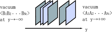
Figure 1: Multi-wall connecting vacua $\langle A_{1}A_{2}\cdots A_{N_{\rm C}}\rangle$ and $\langle B_{1}B_{2}\cdots B_{N_{\rm C}}\rangle$.

The BPS equations for hypermultiplet (the first of Eq.(6)) can be solved[9] by defining an element $S(y)$ of a complexified gauge group $GL(N_{\rm C},\mathbf{C})$ as

$$\Sigma+iW_{y}\equiv S^{-1}(y)\partial_{y}S(y),\qquad H(y)=S^{-1}(y)H_{0}e^{My}.$$ (7)

We call the constant $N_{\rm C}\times N_{\rm F}$ matrix $H_{0}$ “ moduli matrix”.

With the above solution, we can rewrite the vector multiplet BPS equation into the following equation in terms of the gauge invariant quantity $\Omega\equiv SS^{\dagger}$

$$\partial_{y}\left(\Omega^{-1}\partial_{y}\Omega\right)=g^{2}c\left(\mathbf{1}_{N_{\rm C}}-\Omega^{-1}\Omega_{0}\right),\qquad\Omega_{0}\equiv c^{-1}H_{0}e^{2My}H_{0}^{\dagger}.$$ (8)

We call this equation “master equation”. The index theorem[10] shows that the number of moduli parameters contained in the moduli matrix $H_{0}$ is just enough, implying that the solution of the master equation exists and is unique for a given $\Omega_{0}$. The existence and uniqueness have been proved rigorously for the case of $U(1)$ gauge theory[11].

Since the solution $S(y)$ of Eq.(7) has $N_{\rm C}^{2}$ integration constants, two sets $(S,H_{0})$ and $(S^{\prime},H_{0}{}^{\prime})$ give the same $H=S^{-1}H_{0}e^{My}$, if they are related by the following global $GL(N_{\rm C},\mathbf{C})$ transformation $V$ (called the $V$-transformation),

$$S\rightarrow S^{\prime}=VS,\quad H_{0}\rightarrow H_{0}{}^{\prime}=VH_{0},\qquad V\in GL(N_{\rm C},\mathbf{C}).$$ (9)

Therefore the genuine moduli parameters of domain walls are given by the equivalence class defined by the $V$-transformation. We thus find that the total moduli space for (multi-)wall solutions is the complex Grassmann manifold[9]:

$${\cal M}_{N_{\rm F},N_{\rm C}} = \{H_{0}|H_{0}\sim VH_{0},V\in GL(N_{\rm C},\mathbf{C})\}\equiv G_{N_{\rm F},N_{\rm C}}$$ (10)

$$\simeq {SU(N_{\rm F})\over SU(N_{\rm C})\times SU(N_{\rm F}-N_{\rm C})\times U(1)}.$$

This is a compact (closed) set of complex dimension $N_{\rm C}\tilde{N}_{\rm C}\equiv N_{\rm C}(N_{\rm F}-N_{\rm C})$. We did not put any boundary conditions at $y\to\pm\infty$ to get the moduli space (10). Therefore it contains configurations with all possible boundary conditions, and can be decomposed into the sum of topological sectors

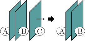
Figure 2: A three wall solution connecting vacuum A to C through B (left). By letting the right-most wall to infinity, we obtain a two wall solution connecting vacuum A to B.

$${\cal M}^{\rm total}_{\rm wall}=\sum_{\rm BPS}{\cal M}^{\langle A_{1},\cdots,A_{N_{\rm C}}\rangle\leftarrow\langle B_{1},\cdots,B_{N_{\rm C}}\rangle}.$$ (11)

As shown in Fig. 2, by sending one of the wall to infinity, we obtain one less walls. Namely the boundaries of a topological sector consists of topological sectors with one less wall. It is interesting to observe that this natural compactification of the moduli space of walls leads to the compact total moduli space (10) for the 1/2 BPS solutions, if we add vacua as points to compactify the manifold.

Components of the moduli matrix $H_{0}$ represent weights of the vacua.

Figure 3: Rapid change of hypermultiplets indicates the positions of walls.

For instance, the moduli matrix for the $U(1)$ gauge theory can be parametrized by $H_{0}=(e^{r_{1}},e^{r_{2}},\cdots,e^{r_{N_{F}}})$. Then the hypermultiplets are given by

$$H=S^{-1}H_{0}e^{My}=S^{-1}(e^{r_{1}+m_{1}y},\cdots,e^{r_{N_{F}}+m_{N_{F}}y})$$ (12)

We see that wall separating $i$- and $i+1$-th vacua is located where the magnitudes of the $i$- and $i+1$-th components become equal as illustrated in Fig. 3. The wall position $y$ is

$${\rm Re}r_{i}+m_{i}y\sim{\rm Re}r_{i+1}+m_{i+1}y\to y=-{\rm Re}(r_{i}-r_{i+1})/(m_{i}-m_{i+1}).$$ (13)

The imaginary part ${\rm Im}(r_{i}-r_{i+1})$ gives the relative phase of the two adjacent vacua. We see that there are $N_{\rm F}-1$ walls maximally. Similarly, the number of walls in non-Abelian $U(N_{\rm C})$ gauge theory is given by $N_{\rm C}(N_{\rm F}-N_{\rm C})$, and each wall carries two moduli, position and relative phase of adjacent vacua.

The low-energy effective Lagrangian on domain walls is given by promoting the moduli parameters in the moduli matrix $H_{0}$ to fields on the world volume of the soliton and by assuming the weak dependence on the world volume coordinates. We assume the slow-movement of moduli fields compared to the two typical mass scales $g\sqrt{c}$ and $\Delta m$ of the wall of hypermultiplets

$$\lambda\ll{\rm min}(\Delta m,g\sqrt{c}).$$ (14)

We find it extremely useful to use the superfield formalism maintaining the preserved four SUSY manifest. The effective Lagrangian for the $1/2$ BPS domain walls is given in terms of the solution $\Omega_{\rm sol}(y,\phi,\phi^{*})$ of the master equation

$${\cal L}=-T_{\rm w}+\int d^{4}\theta K(\phi,\phi^{*})+{\rm higher}\;{\rm derivatives},$$ (15)

where $T_{\rm w}$ is the tension of the domain wall, and $K$ is the Kähler potential of moduli fields $\phi,\phi^{*}$, given by[12]

$$\!\!\!K(\phi,\phi^{*})\!=\!\!\int\!dy\left[c\log{\rm det}\Omega+c{\rm Tr}\left(\Omega_{0}\Omega^{-1}\right)+{1\over 2g^{2}}{\rm Tr}\left({\Omega}^{-1}\partial_{y}\Omega\right)^{2}\right]\Big{|}_{\Omega=\Omega_{\rm sol}}$$ (16)

One of the merit of our superfield formulation is that Kähler potential can be obtained directly without going through Kähler metric and integrating it. We find that the Kähler potential serves as the action for $\Omega$ to obtain the master equation (8).

Let us make some comments. If we take the strong gauge coupling limit $g^{2}c/(\Delta m)^{2}\gg 1$, the model becomes a nonlinear sigma model[13] and the master equation (8) can be solved algebraically

$$\Omega=\Omega_{0}\equiv c^{-1}H_{0}e^{2My}H_{0}^{\dagger}.$$ (17)

The domain wall configuration in our system can be realized as a bound state of kinky D$p$-brane and D($p+4$)-branes in the type II string theories[14]. By doing so ample dynamics of walls have been uncovered. We have found that the moduli space of domain walls is generally the Lagrangian submanifold of the vacuum manifold of corresponding massless model[15].

3 $1/2$ BPS Vortices

Vortices can exist in $5+1$ dimensions or lower. In particular they carry non-Abelian orientational moduli in massless theory[16, 17] as instantons. For simplicity let us consider the case of $N_{\rm F}=N_{\rm C}=N$. Taking the Lagrangian (2) in $5+1$ dimensions, and requiring the half of SUSY to be preserved, we obtain the $1/2$ BPS equations for vortices as

$$0={\cal D}_{1}H+i{\cal D}_{2}H,\quad 0=F_{12}+{g^{2}\over 2}(c{\bf 1}_{N}-HH^{\dagger}).$$ (18)

Hypermultiplet BPS equation can be easily solved in terms of a complexified gauge transformation $S(z,\bar{z})\in GL(N_{\rm C},\mathbf{C})$ and the holomorphic moduli matrix $H_{0}(z)$[18, 19]

$$H=S^{-1}H_{0}(z),\quad W_{1}+iW_{2}=-i2S^{-1}{\bar{\partial}}_{z}S,\quad z\equiv x^{1}+ix^{2}.$$ (19)

The vector multiplet BPS equation can be transformed to the following master equation

$$\partial_{z}(\Omega^{-1}\bar{\partial}_{z}\Omega)={g^{2}\over 4}(c{\bf 1}_{N}-\Omega^{-1}H_{0}H_{0}^{\dagger}).$$ (20)

The solutions of the BPS equation saturate the BPS bound for the energy density for vorticity $k\in{\bf Z}_{\geq 0}$

$$T\equiv-c\int d^{2}x\ {\rm Tr}F_{12}=2\pi ck=-i{c\over 2}\oint dz\ \partial{\rm log}({\rm det}H_{0})+{\rm c.c.},$$ (21)

with the boundary condition ${\rm det}(H_{0})\sim z^{k}$ at $z\to\infty$. The moduli matrices $H_{0}(z)$ related by the $V$-transformation give identical physical fields : $H_{0}\to VH_{0}$, $S\to VS$, $V=V(z)\in GL(N,{\bf C}),\det V=$ const.$\neq 0$. Therefore, the moduli space for vortices is found as

$${\cal M}_{k,N}={\left\{H_{0}(z)|H_{0}(z)\in M_{N},{\rm deg}\,{\rm det}(H_{0}(z))=k\right\}\over\left\{V(z)|V(z)\in M_{N},{\rm det}V(z)={\rm const.}\not=0\right\}}.$$ (22)

The generic points of moduli space has ${\rm dim}({\cal M}_{N,k})=2kN$ and can be represented by

$$H_{0}=\left(\begin{array}[]{cc}{\bf 1}_{N-1}&-\vec{R}(z)\\ 0&P(z)\end{array}\right),\quad P(z)=\prod_{i=1}^{k}(z-z_{i}).$$ (25)

Moduli space of a single vortex $k=1$ is given[16, 17] by ${\cal M}_{N,k=1}$ $\simeq$ ${\bf C}\times{\bf C}P^{N-1}$ and is represented by the moduli matrix (25) with $\vec{R}^{T}=(b_{1},\cdots,b_{N-1})$ and $P(z)=z-z_{0}$. Moduli space of $k$ separated vortices is given by a symmetric product $\left({\bf C}\times{\bf C}P^{N-1}\right)^{k}/\mathfrak{S}_{k}$. The orbifold singularities of this are appropriately resolved in the full moduli space[19]. We also find that the Kähler quotient construction[16] can also be obtained from our moduli matrix by a change of basis. Superfield formulation with the slow-movement expansion readily yields the effective Lagrangian on the world volume of vortices[12]. The duality between vortices and walls has been discussed[20].

4 1/4 BPS Webs of Domain Walls

The direction of BPS walls are related to the phase of the hypermultiplet masses. If we have complex masses $\mu_{A}=m_{A}+in_{A}$, we can obtain two or more non-parallel walls, which can lead to wall junctions[21]. We consider the Lagrangian (2) in $3+1$ dimensions, since complex masses can be realized in $3+1$ dimensions or lower

$$M_{1}={\rm diag}\left(m_{1},m_{2},\cdots,m_{N_{\rm F}}\right),\quad M_{2}={\rm diag}\left(n_{1},n_{2},\cdots,n_{N_{\rm F}}\right).$$ (26)

The wall junctions can be realized as a solution of the following $1/4$ BPS equations[22]

$$F_{12}=i\left[\Sigma_{1},\Sigma_{2}\right],\quad{\cal D}_{1}\Sigma_{2}={\cal D}_{2}\Sigma_{1},\quad{\cal D}_{\alpha}H=HM_{\alpha}-\Sigma_{\alpha}H,$$ (27)

$${\cal D}_{1}\Sigma_{1}+{\cal D}_{2}\Sigma_{2}={g^{2}\over 2}(c{\bf 1}_{N_{\rm C}}-HH^{\dagger}).$$ (28)

The solutions saturate the Bogomol’nyi bound for the energy density

$${\cal E} \geq {\cal Y}+{\cal Z}_{1}+{\cal Z}_{2}+\sum_{\alpha=1,2}\partial_{\alpha}J_{\alpha},\quad J_{\alpha}\equiv{\rm Tr}\Big{[}H(M_{\alpha}H^{\dagger}-H^{\dagger}\Sigma_{\alpha})\Big{]},$$ (29)

$${\cal Y}\equiv\frac{2}{g^{2}}\partial_{\alpha}{\rm Tr}\left(\epsilon^{\alpha\beta}\Sigma_{2}{\cal D}_{\beta}\Sigma_{1}\right),\quad{\cal Z}_{1}\equiv c\partial_{1}{\rm Tr}\Sigma_{1},\quad{\cal Z}_{2}\equiv c\partial_{2}{\rm Tr}\Sigma_{2}.$$ (30)

The first two equations in Eq.(27) assures the integrability of the last one in Eq.(27), which is solved by[22]

$$H=S^{-1}H_{0}e^{M_{1}x^{1}+M_{2}x^{2}},\quad W_{\alpha}-i\Sigma_{\alpha}=-iS^{-1}\partial_{\alpha}S,\quad\alpha=1,2.$$ (31)

The remaining BPS equation (28) can be rewritten in terms of the gauge invariant quantity $\Omega\equiv SS^{\dagger}$ as the master equation

$$\sum_{\alpha=1,2}\partial_{\alpha}\left(\partial_{\alpha}\Omega\Omega^{-1}\right)=cg^{2}\left({\bf 1}_{N_{\rm C}}-c^{-1}H_{0}e^{2(M_{1}x^{1}+M_{2}x^{2})}H_{0}^{\dagger}\Omega^{-1}\right),$$ (32)

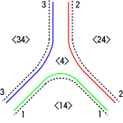
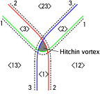
(a) Abelian junction		(b) non-Abelian junction

Figure 4: Internal structures of the junctions with $g\sqrt{c}\ll|\Delta m+i\Delta n|$

The total moduli space of $1/4$ BPS equations (27), (28) can be decomposed into $1/4$, $1/2$, and $1/1$ BPS sectors

$${\cal M}^{\rm webs}_{\rm tot} \simeq G_{N_{\rm F},N_{\rm C}}=\{H_{0}\ |\ H_{0}\sim VH_{0},\ V\in GL(N_{\rm C},{\bf C})\}$$ (33)

$$= {\cal M}^{\text{webs}}_{1/4}\ \bigcup\ {\cal M}^{\text{walls}}_{1/2}\ \bigcup\ {\cal M}^{\text{vacua}}_{1/1}.$$

We find that Abelian gauge theory gives only Abelian junctions with the negative junction charge ${\cal Y}<0$, whereas non-Abelian gauge theory gives non-Abelian junction with positive junction charge ${\cal Y}>0$ in addition to Abelian junction. Physical interpretation of the positive junction charge is the presence of the Hitchin vortex residing at the junction as illustrated in Fig. 4. We also find that there are cases with vanishing junction charge ${\cal Y}=0$ corresponding to the intersections of penetrable walls.

We find that the normalizable moduli of web of walls are given by loops in web as shown in Fig. 5.

(a) grid diagram		(b) energy density ($g^{2}\to\infty$)

Figure 5: Abelian junction with $1$ loop and $3$ external walls in $N_{\rm C}=1,N_{\rm F}=4$ model.

The moduli matrix of $N_{\rm F}=4,N_{\rm C}=1$ case with $M={\rm diag}(1,i,-1-i,0)$ can be parametrized by

$$H_{0}=\sqrt{c}\left(e^{a_{1}+ib_{1}},e^{a_{2}+ib_{2}},e^{a_{3}+ib_{3}},e^{a_{4}+ib_{4}}\right),$$ (34)

with $a_{j}+ib_{j},j=1,2,3$ as external wall moduli, and $a_{4}+ib_{4}$ as the loop moduli, corresponding to the normalizable mode. Grid diagrams are found to be useful to specify the moduli of the web of walls as illustrated in Fig. 5. A brane configuration is proposed in [23].

5 1/4 BPS Monopoles (Instantons) inside a vortex

Vacua outside of monopoles are in the Coulomb phase with unbroken $U(1)$ gauge group. In our $U(N_{\rm C})$ gauge theory with $N_{\rm F}(\geq N_{\rm C})$ flavors of hypermultiplets in the fundamental representation, vacua are in the Higgs phase. If we place a monopole in the Higgs phase, magnetic flux emanating from the monopole is squeezed into vortices, as illustrated in Fig. 6.

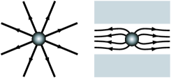
Figure 6: Monopole in Coulomb phase (left) and in Higgs phase (right).

Therefore monopoles in the Higgs phase become composite of monopoles and vortices[24]. Monopoles depend on $x^{1},x^{2},x^{3}$ coordinates and preserve $1/2$ SUSY defined by $\gamma^{123}\varepsilon^{i}=\varepsilon^{i}$. Vortices along $x^{3}$-axis preserve another $1/2$ SUSY defined by $\gamma^{12}(i\sigma_{3})^{i}{}_{j}\varepsilon^{j}=\varepsilon^{i}$. If they coexist as a monopole in the Higgs phase, $1/4$ of SUSY is preserved. $\gamma^{3}(i\sigma_{3})^{i}{}_{j}\varepsilon^{j}=\varepsilon^{i}$. We found that this $1/4$ SUSY precisely allows domain walls perpendicular to the vortices[18].

Let us consider $U(N_{\rm C})$ gauge theory in $4+1$ dimensions and assume field configurations of monopole-vortex-wall composite to depend on $x^{m}\equiv(x^{1},x^{2},x^{3})$ and Poincaré invariance in $x^{0},x^{4}$ space. With the above preserved $1/4$ SUSY, we obtain the $1/4$ BPS equations :

$${\cal D}_{3}\Sigma = {g^{2}\over 2}\left(c{\bf 1}_{N_{\rm C}}-HH{}^{\dagger}\right){+F_{12}},\quad{\cal D}_{3}H=-\Sigma H+HM,$$ (35)

which amounts to the contribution of vortex magnetic field $F_{12}$ added to the wall BPS equation. These are supplemented by the BPS equations for vortices

$$0 = {\cal D}_{1}H+i{\cal D}_{2}H,\quad 0=F_{23}-{\cal D}_{1}\Sigma,\quad 0=F_{31}-{\cal D}_{2}\Sigma.$$ (36)

The solutions of these BPS equations saturate the BPS bound of the energy density

$${\cal E}\geq t_{\rm w}+t_{\rm v}+t_{\rm m}+\partial_{m}J_{m},$$ (37)

where $J_{m}$ is the current that does not contribute to the topological charge, and $t_{\rm w},\,t_{\rm v}$ and $t_{\rm m}$ are energy densities for walls, vortices and monopoles

$${t_{\rm w}}={c\partial_{3}{\rm Tr}(\Sigma)},\quad{t_{\rm v}}={-c{\rm Tr}(F_{12})},\quad{t_{\rm m}}={\frac{2}{g^{2}}\partial_{m}{\rm Tr}(\frac{1}{2}\epsilon^{mnl}\!F_{nl}\Sigma)}.$$ (38)

Integrability condition $[{\cal D}_{1}+i{\cal D}_{2},\,{\cal D}_{3}+\Sigma]=0$ coming from the second and third equations in (36) assures the existence of an invertible complex matrix function $S(x^{m})\in GL(N_{\rm C},\mathbf{C})$ defined by[18]

$$({\cal D}_{3}+\Sigma)S^{-1}=0\rightarrow\Sigma+iW_{3}\equiv S^{-1}\partial_{3}S,$$ (39)

$$({\cal D}_{1}+i{\cal D}_{2})S^{-1}=0\rightarrow W_{1}+iW_{2}\equiv-2iS^{-1}\bar{\partial}S,$$ (40)

where $z\equiv x^{1}+ix^{2}$, and $\bar{\partial}\equiv\partial/\partial z^{*}$. With this matrix function, the BPS Eq. for hypermultiplet is solved by

$$H=S^{-1}(z,z^{*},x^{3})H_{0}(z)e^{Mx^{3}},$$ (41)

where the moduli matrix $H_{0}(z)$: $N_{\rm C}\times N_{\rm F}$ matrix is a holomorphic function of $z$.

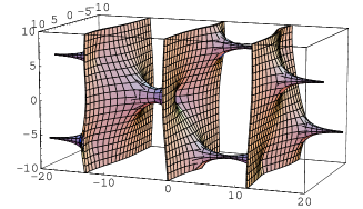
Figure 7: Surfaces defined by the same energy density with $t_{\rm w}+t_{\rm v}=0.5c$.

The remaining BPS equation is rewritten into a master equation for $\Omega\equiv SS^{\dagger}$ with $\Omega_{0}\equiv H_{0}\,e^{2My}H_{0}{}^{\dagger}$ as input data[18]

$$4\partial(\Omega^{-1}\bar{\partial}\Omega)+\partial_{3}(\Omega^{-1}\partial_{3}\Omega)=g^{2}\left(c-\Omega^{-1}\Omega_{0}\right).$$ (42)

We can obtain exact solutions at strong coupling limit: $g^{2}\rightarrow\infty$, since the master equation reduces to an algebraic equation

$$\Omega=\Omega_{0}\equiv c^{-1}H_{0}e^{2My}H_{0}^{\dagger}.$$ (43)

Our construction produces rich contents, even for $U(1)$ gauge theory whose moduli matrix is given by

$$H_{0}(z)=\sqrt{c}\left(f^{1}(z),\,\dots,f^{N_{\rm F}}(z)\right),\quad\Omega=\sum_{A=1}^{N_{\rm F}}|f^{A}(z)|^{2}e^{2m_{A}x^{3}}.$$ (44)

Nonconstant $f^{A}(z)$ can be interpreted as wall positions to depend on $z$. In particular, walls are bent to form vortices, if $f^{A}(z)$ has zeroes. If $f^{A}(z)\propto(z-z^{A}_{\alpha})^{k^{A}_{\alpha}}$, we obtain vorticity $k_{\alpha}^{A}$ at $z=z^{A}_{\alpha}$ on the $A$-th wall. An illustrative configuration of monopoles-vortices-walls is given in Fig. 7. A monopole in Higgs phase is realized as a kink on a vortex, whereas instantons inside a vortex is realized as a vortex on a vortex[25].

The moduli matrix approach is powerful enough to establish interaction rules of monopoles, vortices, and walls. In $U(2)$ gauge theory with $N_{\rm F}=3$ flavors, we can list up all possible moduli matrices for a single vortex in both sides of a wall ($M={\rm diag}(m_{1},m_{2},m_{3})$ ordered as $m_{1}>m_{2}>m_{3}$)

$$\left(\begin{array}[]{ccc}z-z_{2}&a_{2}(z-z_{3})&0\\ 0&0&1\end{array}\right)e^{Mx^{3}},\quad\left(\begin{array}[]{ccc}1&a_{3}&0\\ 0&0&z-z_{4}\end{array}\right)e^{Mx^{3}},$$ (49)

$$\left(\begin{array}[]{ccc}1&a_{1}&b\\ 0&0&z-z_{1}\end{array}\right)e^{Mx^{3}}\sim\left(\begin{array}[]{ccc}\frac{1}{a_{1}}(z-z_{1})&z-z_{1}&0\\ \frac{1}{b}&\frac{a_{1}}{b}&1\end{array}\right)e^{Mx^{3}}.$$ (54)

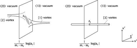
Figure 8: The vortex positions can separate on domain wall

Moduli matrices in (49) are essentially those in $U(1)$ gauge theory. The first one has two vortices at $z=z_{2},z_{3}$ stretching to opposite directions as in the left of Fig. 8. The second one represents a single vortex penetrating the wall as in the right of Fig. 8. We see that vortices can end on a wall in different positions as long as monopole does not sit on any of the vortices. The moduli matrix in Eq.(54) is intrinsically non-Abelian and gives the configuration depicted in Fig. 9. We find that monopole can penetrate through a wall as long as the position of vortices on both sides of the wall coincide. Vortices on a wall can separate only when the monopole is removed to infinity.

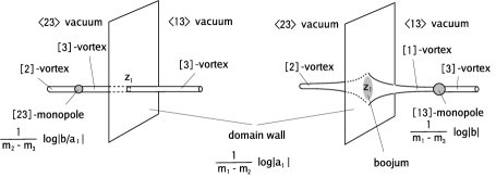
Figure 9: Monopole can go through wall only if vortex positions on the wall coincide.

We find that these $1/4$ BPS composite solitons are related by the Scherk-Schwarz dimensional reduction from $5+1$ dimensions to $4+1$ or $3+1$ dimensions as the table below. Dyonic extension of these solitons are also discussed [26].

dim $\setminus$ charge	positive	negative
$d=5,6$ instanton	Instanton inside vortex	Intersecton[25]
$d=4,5$ monopole	Monopole attached by vortices	Boojum[18, 10]
$d=3,4$ Hitchin	Non-Abelian wall junction	Abelian wall junction[22]

6 Conclusion

1. The BPS solitons are constructed in SUSY $U(N_{\rm C})$ gauge theories with $N_{\rm F}$ hypermultiplets in the fundamental representation.

2. Total moduli space of the non-Abelian walls is given by a compact complex Grassmann manifold described by the moduli matrix $H_{0}$.

3. A general formula for the effective Lagrangian is obtained.

4. Webs of domain walls are obtained. There are Abelian and non-Abelian junctions of walls in non-Abelian gauge theory. Normalizable moduli of the web of walls are associated with loops of walls.

5. Composite $1/4$ BPS solitons in Higgs phase are systematically obtained by Scherk-Schwarz dimensional reduction: instanton-vortex-vortex, wall-vortex-monopole, webs of walls.

6. All possible $1/4$ BPS solutions are obtained exactly and explicitly in the strong gauge coupling limit.

References

- [1] M. Eto, Y. Isozumi, M. Nitta, K. Ohashi and N. Sakai, J. Phys. A 39 (2006) R315 [arXiv:hep-th/0602170].
- [2] P. Horava and E. Witten, Nucl. Phys. B 475 (1996) 94 [arXiv:hep-th/9603142].
- [3] N. Arkani-Hamed, S. Dimopoulos and G. R. Dvali, Phys. Lett. B 429 (1998) 263 [arXiv:hep-ph/9803315]; I. Antoniadis, N. Arkani-Hamed, S. Dimopoulos and G. R. Dvali, Phys. Lett. B 436 (1998) 257 [arXiv:hep-ph/9804398].
- [4] L. Randall and R. Sundrum, Phys. Rev. Lett. 83 (1999) 3370 [arXiv:hep-ph/9905221]; Phys. Rev. Lett. 83 (1999) 4690 [arXiv:hep-th/9906064].
- [5] E. B. Bogomolny, Sov. J. Nucl. Phys. 24 (1976) 449 [Yad. Fiz. 24 (1976) 861]; M. K. Prasad and C. M. Sommerfield, Phys. Rev. Lett. 35 (1975) 760.
- [6] E. Witten and D. I. Olive, Phys. Lett. B 78 (1978) 97.
- [7] N. Seiberg and E. Witten, Nucl. Phys. B 426 (1994) 19 [Erratum-ibid. B 430 (1994) 485] [arXiv:hep-th/9407087]; Nucl. Phys. B 431 (1994) 484 [arXiv:hep-th/9408099].
- [8] P. Fayet and J. Iliopoulos, Phys. Lett. B 51 (1974) 461.
- [9] Y. Isozumi, M. Nitta, K. Ohashi and N. Sakai, Phys. Rev. Lett. 93 (2004) 161601 [arXiv:hep-th/0404198]; Phys. Rev. D 70 (2004) 125014 [arXiv:hep-th/0405194].
- [10] N. Sakai and D. Tong, JHEP 0503 (2005) 019 [arXiv:hep-th/0501207].
- [11] N. Sakai and Y. Yang, Comm. Math. Phys. (in press) [arXiv:hep-th/0505136].
- [12] M. Eto, Y. Isozumi, M. Nitta, K. Ohashi and N. Sakai, Phys. Rev. D 73 (2006) 125008 [arXiv:hep-th/0602289].
- [13] M. Arai, M. Naganuma, M. Nitta and N. Sakai, Nucl. Phys. B 652 (2003) 35 [arXiv:hep-th/0211103].
- [14] M. Eto, Y. Isozumi, M. Nitta, K. Ohashi, K. Ohta and N. Sakai, Phys. Rev. D 71 (2005) 125006 [arXiv:hep-th/0412024].
- [15] M. Eto, Y. Isozumi, M. Nitta, K. Ohashi, K. Ohta, N. Sakai and Y. Tachikawa, Phys. Rev. D 71 (2005) 105009 [arXiv:hep-th/0503033].
- [16] A. Hanany and D. Tong, JHEP 0307 (2003) 037 [arXiv:hep-th/0306150].
- [17] R. Auzzi, S. Bolognesi, J. Evslin, K. Konishi and A. Yung, Nucl. Phys. B 673 (2003) 187 [arXiv:hep-th/0307287].
- [18] Y. Isozumi, M. Nitta, K. Ohashi and N. Sakai, Phys. Rev. D 71 (2005) 065018 [arXiv:hep-th/0405129].
- [19] M. Eto, Y. Isozumi, M. Nitta, K. Ohashi and N. Sakai, Phys. Rev. Lett. 96 (2006) 161601 [arXiv:hep-th/0511088].
- [20] M. Eto, T. Fujimori, Y. Isozumi, M. Nitta, K. Ohashi, K. Ohta and N. Sakai, Phys. Rev. D 73 (2006) 085008 [arXiv:hep-th/0601181].
- [21] G. W. Gibbons and P. K. Townsend, Phys. Rev. Lett. 83 (1999) 1727 [arXiv:hep-th/9905196]; S. M. Carroll, S. Hellerman and M. Trodden, Phys. Rev. D 61 (2000) 065001 [arXiv:hep-th/9905217]; H. Oda, K. Ito, M. Naganuma and N. Sakai, Phys. Lett. B 471 (1999) 140 [arXiv:hep-th/9910095]; K. Ito, M. Naganuma, H. Oda and N. Sakai, Nucl. Phys. B 586 (2000) 231 [arXiv:hep-th/0004188]; Nucl. Phys. Proc. Suppl. 101 (2001) 304 [arXiv:hep-th/0012182]; A. Gorsky and M. A. Shifman, Phys. Rev. D 61 (2000) 085001 [arXiv:hep-th/9909015]; M. Naganuma, M. Nitta and N. Sakai, Phys. Rev. D 65 (2002) 045016 [arXiv:hep-th/0108179]; K. Kakimoto and N. Sakai, Phys. Rev. D 68 (2003) 065005 [arXiv:hep-th/0306077].
- [22] M. Eto, Y. Isozumi, M. Nitta, K. Ohashi and N. Sakai, Phys. Rev. D 72 (2005) 085004 [arXiv:hep-th/0506135]; Phys. Lett. B 632 (2006) 384 [arXiv:hep-th/0508241].
- [23] M. Eto, Y. Isozumi, M. Nitta, K. Ohashi, K. Ohta and N. Sakai, AIP Conf. Proc. 805 (2006) 354 [arXiv:hep-th/0509127].
- [24] D. Tong, Phys. Rev. D 69 (2004) 065003 [arXiv:hep-th/0307302]; R. Auzzi, S. Bolognesi, J. Evslin and K. Konishi, Nucl. Phys. B 686 (2004) 119 [arXiv:hep-th/0312233]; M. Shifman and A. Yung, Phys. Rev. D 70 (2004) 045004 [arXiv:hep-th/0403149]; A. Hanany and D. Tong, JHEP 0404 (2004) 066 [arXiv:hep-th/0403158].
- [25] M. Eto, Y. Isozumi, M. Nitta, K. Ohashi and N. Sakai, Phys. Rev. D 72 (2005) 025011 [arXiv:hep-th/0412048].
- [26] K. Lee and H. U. Yee, Phys. Rev. D 72 (2005) 065023 [arXiv:hep-th/0506256]; M. Eto, Y. Isozumi, M. Nitta and K. Ohashi, Nucl. Phys. B (in press) [arXiv:hep-th/0506257].