Cancellation of energy-divergences and renormalizability in Coulomb gauge QCD within the Lagrangian formalism

Abstract

In Coulomb gauge QCD in the Lagrangian formalism, energy divergences arise in individual diagrams. We give a proof on cancellation of these divergences to all orders of perturbation theory without obstructing the algebraic renormalizability of the theory.

I Introduction

In nonabelian gauge theories, the Coulomb gauge is one of the most important ones. The theories with this gauge are described in terms of physical fields, so that the unitarity is manifest. In the Lagrangian, second-order, formalism of Coulomb gauge perturbation theory, there appear, at one-loop order and above, divergent energy integrals of the form,

$$\int\frac{dp_{0}}{2\pi}\,F({\bf p},...)\,.$$ (1.1)

Here $p_{0}$ is the temporal component of the four-momentum $P^{\mu}=(p_{0},{\bf p})$ and “…” indicates a set of external three momenta of the amplitude under consideration. [We use capital letter $Q^{\mu}$ to denote a four vector $Q^{\mu}=(q^{0},{\bf q})$ and $q^{j}$ for denoting a three vector.]

The following results are established by now on the energy divergence problem.

1) In the calculation using the Hamiltonian, phase-space, first order, form of Feynman rules, energy-divergences like (1.1) do not appear doust in the first place.

2) On the basis of a correspondence formula which equates amplitudes in a covariant gauge to those in a gauge without ghosts, Cheng and Tsai CT showed that, when all relevant contributions are added, cancellation should occur between the divergences like (1.1) in the Coulomb gauge.

3) With the aid of an interpolating gauge, which interpolates between a covariant gauge and the Coulomb gauge, it was shown BZ in the phase-space formalism that, when all participating contributions are added, cancellation occurs between the divergences like (1.1). (See, also, doust .)

Furthermore, following two types of ill-defined integrals appear:

$$\int\frac{dp_{0}}{2\pi}\,\frac{p_{0}}{p_{0}^{2}-p^{2}+i0^{+}}\,G({\bf p},...)\,,$$ (1.2)

$$\int\frac{dp_{0}}{2\pi}\frac{dq_{0}}{2\pi}\,\frac{p_{0}}{p_{0}^{2}-p^{2}+i0^{+}}\,\frac{q_{0}}{q_{0}^{2}-q^{2}+i0^{+}}\,H({\bf p},{\bf q},...)\,.$$

(1.3)

The type (1.2) appears at one-loop order and above, and the type (1.3) does at two-loop order and above.

In Coulomb-gauge QCD, one encounters a problem of operator ordering in the Hamiltonian. This problem was resolved by Christ and Lee CL , along the line of the earlier work of Schwinger schw : The quantum Hamiltonian is different from the classical Hamiltonian by special terms, labeled $V_{1}+V_{2}$. Since then, it has been shown that the ill-defined integrals of the form (1.3) are connected doust ; CT1 with these $V_{1}+V_{2}$ terms, and integrals of the form (1.2) can be set equal to zero CT1 .

As mentioned above, when all relevant energy-diverging contributions are added, energy divergences cancel out, provided that the remaining three-momenta integrations are convergent. It has been pointed out DT that, in dealing with the renormalization parts, difficulties arise in simultaneously handling the diverging energy integrations and renormalizing the ultraviolet (UV) divergences. A formal proof of cancellation of energy-divergences and algebraic renormalizability is given in BZ with the aid of an interpolating gauge in the phase-space formalism. Recently, this issue is studied AT in an example in which quark-loop subgraphs are inserted into the second-order gluon self-energy graphs. As mentioned in 1) above, in the phase-space formalism, two integrals over the internal energies converge, provided that the internal three spatial momenta are held fixed. It is found in AT that, when one first computes each subgraphs and performs renormalization, energy-divergences re-appear in the final energy integrals. Thanks to the Ward identity, these energy-divergent contributions are cancelled out when all relevant contributions are added.

In this paper, generalizing the analysis in AT to all orders of perturbation theory, we give a proof of cancellation of energy-divergences without spoiling the renormalizability of the Coulomb-gauge QCD by using the Feynman rules derived from the Lagrangian, second-order, formalism. In dealing with the energy-divergences of the form (1.1), extra $V_{1}+V_{2}$ terms do not participate CT1 , and then we can use the Coulomb-gauge Feynman rules derived from the Lagrangian formalism.

In Sec. II, we derive a power-counting formula for divergent energy integrals. In Sec. III, we show that the energy divergences, Eq. (1.1), are cancelled out to all orders of perturbation theory. In Sec. IV, for completeness, with the help of the power-counting formula obtained in Sec. II, we identify the diagrams that yields ill-defined energy integrals (1.2) and (1.3). In Sec. V, we show that the renormalization does not spoil the cancellation of energy divergences.

II Preliminary

QCD in the Coulomb gauge is defined, with standard notation, by the effective Lagrangian density

$${\cal L}_{\mbox{\scriptsize{eff}}} = -\frac{1}{4}F^{\mu\nu}_{a}F_{\mu\nu}^{a}-\frac{1}{2\alpha}(\partial_{i}A_{a}^{i})(\partial_{j}A_{a}^{j})$$ (2.1)

$$+\partial_{i}\bar{\eta}_{a}\left(\delta_{ab}\partial^{i}-gf_{acb}A^{i}_{c}\right)\eta_{b}$$

$$+\bar{\psi}\left(i\partial\kern-0.44998pt\raise 1.29167pt\hbox to0.0pt{\hss/}\kern 2.5pt-m-gt_{a}{A\kern-1.00006pt\raise 1.29167pt\hbox to0.0pt{\hss/}\kern 3.50006pt}_{a}\right)\psi\,,$$

where $t_{a}=\lambda_{a}/2$ and $F_{a}^{\mu\nu}=\partial^{\mu}A_{a}^{\nu}-\partial^{\nu}A_{a}^{\mu}-gf_{abc}A^{\mu}_{b}A^{\nu}_{c}$. Here $A_{a}^{\mu}$ denotes the gluon field and $\eta_{a}$ ($\bar{\eta}_{a}$) denotes the (anti)FP-ghost field. We have introduced one quark flavor ($\psi,\bar{\psi}$). Generalization to the case with several quark flavors is straightforward. Generalization to other nonabelian gauge theories is also straightforward.

Throughout in the sequel, we restrict ourselves to the strict Coulomb gauge ($\alpha\to 0$). The propagators in the Lagrangian formalism may be extracted from the bilinear terms (in fields) of ${\cal L}_{\mbox{\scriptsize{eff}}}$ in Eq. (2.1);

$$\langle\mbox{T}A_{a}^{i}(x)A_{b}^{j}(y)\rangle \stackrel{{\scriptstyle F.T.}}{{\longrightarrow}} i\delta_{ab}\frac{\delta^{ij}_{\perp}({\bf p})}{P^{2}+i0^{+}}\equiv i\delta_{ab}D^{ij}(P)\,,$$

$$\langle\mbox{T}A_{a}^{0}(x)A_{b}^{0}(y)\rangle \stackrel{{\scriptstyle F.T.}}{{\longrightarrow}} i\delta_{ab}\frac{1}{p^{2}}\equiv i\delta_{ab}D^{00}(p)\,,$$

$$\langle\mbox{T}\eta_{a}(x)\bar{\eta}_{b}(y)\rangle \stackrel{{\scriptstyle F.T.}}{{\longrightarrow}} -i\delta_{ab}\frac{1}{p^{2}}\equiv i\delta_{ab}\tilde{D}(p)\,.$$ (2.2)

Here, $P^{2}=p_{0}^{2}-p^{2}$ $(p=|{\bf p}|)$, $\delta_{\perp}^{ij}({\bf p})\equiv\delta^{ij}-p^{i}p^{j}/p^{2}$, and ‘F.T.’ stands for taking Fourier transformation.

Superficial degree of energy divergence

It is sufficient to deal with one particle irreducible diagrams. ¿From them, we take a particular diagram $G$. We introduce the following abbreviations;

i) ‘$A$’ for the spatial component of the gluon field, $A_{a}^{i}$, which we call the transverse gluon (tgluon) in the sequel,

ii) ‘$0$’ for the temporal component of the gluon field, $A^{0}_{a}$, which we call the ‘Coulomb’,

iii) ‘$G$’ (‘$\bar{G}$’) for the (anti)FP-ghost,

iv) ‘$q$’ (‘$\bar{q}$’) for the (anti)quark.

We adopt the following notation to describe the diagram $G$:

$$I_{i}=\mbox{ number of internal lines of }i\;\;\;\;\;(i=A,0,G,q)\,,$$

$$E_{i}=\mbox{ number of external lines of }i$$

$$\mbox{\hskip 129.16626pt}(i=A,0,G,q\;\mbox{and}\;\bar{q})\,,$$

$$V_{3A},V_{4A},V_{AA0},V_{A00},V_{AA00},V_{A\bar{G}G},V_{A\bar{q}q},V_{0\bar{q}q}$$

$$\mbox{\hskip 10.76385pt}=\mbox{number of vertices indicated by the suffices}\,.$$

Let us find the superficial degree of energy divergence, $\omega(G)$, of $G$. When $\omega(G)\leq-1$, energy integral converges.

To $\omega(G)$, each loop contributes $+1$, each internal tgluon line contributes $-2$, each internal quark line contributes $-1$, and each ‘$AA0$’ vertex contributes $+1$. Then, it is clearly

$$\omega(G)=L-2I_{A}-I_{q}+V_{AA0}\,.$$ (2.3)

¿From the topological structure of $G$, we have

$$L = I_{A}+I_{0}+I_{G}+I_{q}-\left(\sum_{i}V_{i}-1\right)\,,$$

$$2I_{A}+E_{A} = 3V_{3A}+4V_{4A}+2V_{AA0}+V_{A00}$$

$$+2V_{AA00}+V_{A\bar{G}G}+V_{A\bar{q}q}\,,$$

$$2I_{0}+E_{0} = V_{AA0}+2V_{A00}+2V_{AA00}+V_{0\bar{q}q}\,,$$

$$2I_{q}+E_{q\;\mbox{\scriptsize{and}}\;\bar{q}} = 2V_{A\bar{q}q}+2V_{0\bar{q}q}\,,$$

$$2I_{G}+E_{G} = 2V_{A\bar{G}G}\,.$$ (2.4)

In the first equation, summation is taken over all types of vertices in $G$, where we have used the fact that there is energy conservation at each vertex but there is also one overall energy conservation. Using the relations (2.4) in Eq. (2.3), we obtain

$$\omega(G) = 1+\frac{1}{2}\left(E_{A}-V_{AA0}-V_{A00}-2V_{AA00}-V_{A\bar{G}G}\right)$$ (2.5)

$$-\frac{1}{2}\left(E_{G}+E_{0}\right)$$

$$-\frac{1}{2}\left(5V_{3A}+6V_{4A}+3V_{A\bar{q}q}+V_{0\bar{q}q}\right)\,.$$

The directions of the momenta of the external lines are taken toward outside of the diagram $G$ (c.f., Fig. 1). Eq. (2.5) tells us that $\omega(G)\leq 1$.

III Cancellation of $\omega(G)=1$ energy divergences

III.1 Participating diagrams

The diagram $G$ with $\omega(G)=1$ yields the divergent integral of the form (1.1). From Eq. (2.5) we learn that the $\omega(G)=1$ energy-divergence arises only when the following three conditions are simultaneously met:

(C1) $E_{A}=V_{AA0}+V_{A00}+2V_{AA00}+V_{A\bar{G}G}$,

(C2) $E_{0}=E_{G}=0$,

(C3) $V_{3A}=V_{4A}=V_{A\bar{q}q}=V_{0\bar{q}q}=0$.

These conditions leads to the following propositions:

(P1) Energy divergence arises only from the tgluon amplitudes [(C2) and (C3)].

(P2) In an energy-divergent tgluon amplitude, the vertices in (C1) above, $V_{AA0}$, $V_{A00}$, $V_{AA00}$, and $V_{A\bar{G}G}$, are the external vertices, i.e., external-tgluon lines go out from them. In particular, when one tgluon goes out from a vertex $V_{AA00}$, if any, in the diagram $G$, no energy divergence arises [(C1)].

(P3) Energy divergent diagrams do not have internal vertex [(P2) and (C3)].

Then,

(P4) Then, energy divergence can arise only from tgluon one-loop diagrams, Fig. 1.

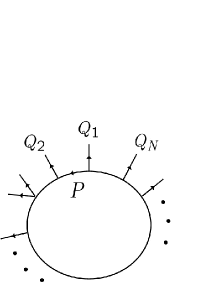
Fig. 1: One-loop N-tgluon diagram.

III.2 Structure of the building blocks of the tgluon one-loop diagrams

Let us compute the amplitude for the diagram in Fig. 2(a) that is a part of Fig. 1:

$${\cal A}_{2a} = \left[-gf_{bce}(p^{0}+q_{2}^{0})\right]\frac{i\delta^{ij}_{\perp}({\bf p})}{P^{2}+i0^{+}}\left[gf_{dae}(q^{0}_{1}-p^{0})\right]$$

$$= ig^{2}f_{bce}f_{dae}\left[1+\frac{p^{2}-(q_{1}^{0}-q_{2}^{0})p^{0}-q_{1}^{0}q_{2}^{0}}{P^{2}+i0^{+}}\right]\delta^{ij}_{\perp}({\bf p})\,.$$

The second term in the square brackets on the last line does not yield the $\omega(G)=1$ energy divergence. Here and throughout in the following we are concerned only with the portions that participate in the $\omega(G)=1$ energy divergence. Then, we have

$${\cal A}_{2a} \simeq ig^{2}f_{bce}f_{dae}\left(\delta^{ij}-\frac{p^{i}p^{j}}{p^{2}}\right)\,,$$ (3.2)

where ‘$\simeq$’ indicates that the right-hand side is the portion of the left-hand side that leads to the energy divergent contribution to the one-loop amplitudes under consideration.

Fig. 2: Lowest order four-point diagrams, each of which is a part of Fig.1. Here Solid lines represent tgluons; dashed lines represent Coulombs; and dot-dashed line represents FP-ghost.

The amplitude for the diagram in Fig. 2(b) reads

$${\cal A}_{2b} = -ig^{2}\left(f_{bce}f_{dae}-f_{bde}f_{ace}\right)\delta^{ij}$$ (3.3)

$$\equiv {\cal A}_{2b}^{(1)}+{\cal A}_{2b}^{(2)}\,.$$

We see from Eqs. (3.2) and (3.3) that the partial cancellation occurs between ${\cal A}_{2a}$ and ${\cal A}_{2b}^{(1)}$. Similar partial cancellation occurs between the contribution from the diagram that is obtained from Fig. 2(a) by $(a,i,Q_{1})\leftrightarrow(b,j,Q_{2})$ and ${\cal A}_{2b}^{(2)}$. Thus, we have

$${\cal A}_{2a}+{\cal A}_{2b}^{(1)}\simeq-ig^{2}f_{bce}f_{dae}\frac{p^{i}p^{j}}{p^{2}}\;\;\;\left(\equiv{\cal A}_{2}\right)\,.$$ (3.4)

With understanding that Figs. 2(a) and 2(b) are always combined into the form (3.4), we will forget Fig. 2(b) or $V_{AA00}$ hereafter.

The contribution from Fig. 2(c) reads

$${\cal A}_{2c} = \left[gf_{bce}(2p^{j}-q_{2}^{j})\right]\frac{i}{p^{2}}\left[gf_{dae}(2p^{i}+q^{i}_{1})\right]$$ (3.5)

$$= 4ig^{2}f_{bce}f_{dae}\frac{p^{i}p^{j}}{p^{2}}\,.$$

Here we have used the fact that, in the strict Coulomb gauge adopted here, $q_{1}^{i}\epsilon^{i}_{r}({\bf q}_{1})=0$ $(r=1,2)$ and $q_{1}^{i}D^{ik}(Q_{1})=0$, where $\epsilon^{i}_{r}({\bf q}_{1})$ and $D^{ik}(Q_{1})$ are, in respective order, the tgluon polarization vector and the propagator, Eq. (2.2), which are to be attached to ${\cal A}_{2c}$. Thus, $q_{1}^{i}$ may be dropped. Similarly, $q_{2}^{j}$ may be dropped.

In a similar manner, we have, for the contribution from Fig. 2(d),

$${\cal A}_{2d} = \left[-gf_{bce}(p^{j}-q^{j}_{2})\right]\frac{-i}{p^{2}}\left[-gf_{dae}p^{i}\right]$$ (3.6)

$$= -ig^{2}f_{bce}f_{dae}\frac{p^{i}p^{j}}{p^{2}}\,.$$

We observe that, besides the difference between the overall factors, the functional forms of ${\cal A}_{2}$, ${\cal A}_{2c}$, and ${\cal A}_{2d}$ are the same. We note that the integrand of a potentially energy divergent tgluon one-loop amplitude is independent of the temporal component of the loop momentum.

Finally in this subsection, it should be emphasized that the one-loop diagram that includes two or more adjacent tgluon propagators does not yield energy divergence (c.f., Eq. (LABEL:2anano)).

III.3 Absence of overlapping energy divergences

Here, we show that no overlapping energy divergences arise. Assume that, in the two-loop diagram depicted in Fig. 3, both the left-side one-loop ($\Xi_{L}$) and the right-side one-loop ($\Xi_{R}$) yield energy divergence. Then, from (P4) above, four lines with momenta $P$, $Q$, $P^{\prime}$, and $Q^{\prime}$ are the tgluon lines. Furthermore, from the observation at the end of Sec. IIIB, the line with momentum $P-Q$ is the $A_{0}$ or Coulomb line. Then, the vertex factor for the vertex at which three lines with momenta $P$, $Q$, and $P-Q$ meet is proportional to $p_{0}+q_{0}$. As can be seen from Eq. (LABEL:2anano), the ‘$p_{0}$’ (‘$q_{0}$’) part participates in the energy divergence for $\Xi_{L}$ ($\Xi_{R}$) but does not participate in the energy divergence for $\Xi_{R}$ ($\Xi_{L}$). Thus, the energy divergence does not arise simultaneously from $\Xi_{L}$ and $\Xi_{R}$.

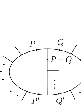
Fig. 3: Two-loop tgluon diagram.

III.4 Cancellation of $\omega(G)=1$ energy divergences

One can read off from Eqs. (LABEL:2anano) - (3.5) the relative factors for the Coulomb- and the tgluon-propagators; $1:-1$, and the relative vertex factors for a $A00$- and $AA0$-vertices; $1:-1/2$. To represent these relative factors, we introduce matrices,

$$\hat{\cal P}=\left(\begin{array}[]{cc}-1&0\\ 0&1\end{array}\right)\,,\;\;\;\;\;\;\hat{\cal V}=\left(\begin{array}[]{cc}0&-1/2\\ -1/2&1\end{array}\right)\,.$$ (3.7)

Here the first rows and columns correspond to ‘$A$’ and the second rows and columns to ‘$0$’. $\hat{\cal V}_{11}=0$ comes from the fact remarked at the end of Sec. IIIB. Let ${\cal A}_{N}^{(G)}$ be the sum of $N$-point tgluon amplitudes for Fig. 1, where the loop consists of Coulomb and/or tgluons lines. Then we obtain for the $\omega(G)=1$ energy-divergent contribution to ${\cal A}_{N}^{(G)}$,

$${\cal A}_{N}^{(G)}\simeq\left[\mbox{Tr}\left(\hat{\cal P}\hat{\cal V}\right)^{N}\right]{\cal A}_{N}^{(G0)}\,,$$ (3.8)

where ${\cal A}_{N}^{(G0)}$ is the contribution from Fig. 1, where all $N$ propagators are the Coulomb ones. Note that, for $N=2$, a symmetry factor $1/2$ is necessary, which is included in ${\cal A}_{N}^{(G)}$ and ${\cal A}_{N}^{(G0)}$. Through mathematical induction, we obtain

$$\left(\hat{\cal P}\hat{\cal V}\right)^{N}=2^{-N}\left(\begin{array}[]{cc}-N+1&N\\ -N&N+1\end{array}\right)\,,$$ (3.9)

so that

$${\cal A}_{N}^{(G)}\simeq 2^{1-N}{\cal A}_{N}^{(G0)}\,.$$ (3.10)

The tgluon amplitude ${\cal A}_{N}^{(FP)}$ for the FP-ghost one-loop diagrams is obtained from ${\cal A}_{N}^{(G0)}$ through the following operations (cf. Eqs. (3.5) and (3.6)); a) change the sign of each propagator, b) multiply a factor $-1/2$ for each vertex, c) multiply a factor $2$, for $3\leq N$, that corresponds to two diagrams with opposite circulation of fermion number, and d) multiply $-1$ that comes from one fermion loop. Thus, we obtain

$${\cal A}_{N}^{(FP)} = (-)\cdot 2\cdot(-)^{N}\cdot\left(-\frac{1}{2}\right)^{N}\cdot{\cal A}_{N}^{(G0)}$$

$$=-2^{1-N}{\cal A}_{N}^{(G0)}\,.$$

For $3\leq N$, the factor ‘2’ in the mid-term comes from c) above. For $N=2$, as mentioned after Eq. (3.8), ${\cal A}_{2}^{(G0)}$ includes a symmetry factor ‘1/2’, while, ${\cal A}_{2}^{(FP)}$ does not include a factor ‘$1/2$’. Then, the factor ‘$2$’ is necessary in the mid-term. Thus, we see that ${\cal A}_{N}^{(G)}$ cancels ${\cal A}_{N}^{(FP)}$:

$${\cal A}_{N}\equiv{\cal A}_{N}^{(G)}+{\cal A}_{N}^{(FP)}\simeq 0\,.$$ (3.11)

III.5 Regularization

As mentioned above, ${\cal A}_{N}^{(G0)}$ is independent of the temporal component of the loop momentum and is of the form (1.1),

$${\cal A}_{N}^{(G0)}=\int d^{3}p\int dp_{0}\,F({\bf p},...)\,.$$ (3.12)

Integration over $p_{0}$ diverges. In order to rigorously handle this integral we should introduce some regularization. It is desirable to adopt the regularization that preserves the BRST symmetry of the theory, so that the regularizing quantum effective action $\Gamma$ satisfies the Zinn-Justin equation, whose explicit form is not necessary for our purpose. To our best knowledge, two candidates are available, i.e., the interpolating gauges BZ , and the split dimensional regularization lei .

Throughout in this paper, we adopt the interpolating gauge BZ , which is defined by introducing the gauge condition,

$$\xi\partial_{0}A_{a}^{0}+\partial_{i}A_{a}^{i}=0$$

($\xi$ is a real parameter). The Coulomb gauge is obtained by taking the limit $\xi\to 0$. $\xi$ here plays a role of regularization of the energy-divergent integrals in the Coulomb gauge. For arbitrary $\xi$, $\Gamma$ satisfies the Zinn-Justin equation, which, in the limit $\xi\to 0$, turns out to be its Coulomb-gauge counterpart.

Gluon- and ghost-propagators read

$$\Delta^{ij}(P) = \frac{1}{P^{2}+i0^{+}}\left[\delta^{ij}-\frac{p^{2}-\xi(2-\xi)p_{0}^{2}}{(P\cdot P_{\xi}+i0^{+})^{2}}p^{i}p^{j}\right]\,,$$

$$\Delta^{00}(P) = \frac{p^{2}}{(P\cdot P_{\xi}+i0^{+})^{2}}\,,$$

$$\Delta^{0i}(P) = \Delta^{i0}=\frac{\xi p_{0}p^{i}}{(P\cdot P_{\xi}+i0^{+})^{2}}\,,$$

$$\tilde{\Delta}(P) = \frac{1}{P\cdot P_{\xi}+i0^{+}}=\frac{P\cdot P_{\xi}}{p^{2}}\Delta^{00}(P)\,,$$ (3.13)

where $P_{\xi}\equiv(\xi p_{0},{\bf p})$.

In the following, we only keep the terms that turn out to the $\omega=1$ energy-divergent ones, and we ignore the terms that tend to $0$ in the limit $\xi\to 0$. In place of Eqs. (3.4), (3.5), and (3.6) we have, in respective order,

$${\cal A}_{2} \simeq -ig^{2}f_{bce}f_{dae}\frac{p^{2}-\xi(2-\xi)p_{0}^{2}}{(P\cdot P_{\xi}+i0^{+})^{2}}p^{i}p^{j}\,,$$ (3.14)

$${\cal A}_{2c} \simeq 4ig^{2}f_{bce}f_{dae}\frac{p^{2}}{(P\cdot P_{\xi}+i0^{+})^{2}}p^{i}p^{j}\,,$$ (3.15)

$${\cal A}_{2d} \simeq ig^{2}f_{bce}f_{dae}\frac{\xi p_{0}^{2}-p^{2}}{(P\cdot P_{\xi}+i0^{+})^{2}}p^{i}p^{j}\,.$$ (3.16)

For obtaining ${\cal A}_{2c}$ for Fig. 2(c), we have used the fact that $q_{1}^{i}\epsilon^{i}_{r}({\bf q}_{1})=O(\xi)$ $(r=1,2)$ and $q_{1}^{i}D^{ik}(Q_{1})=O(\xi)$, where $\epsilon^{i}_{r}({\bf q}_{1})$ and $D^{ik}(Q_{1})$ are, in respective order, the tgluon polarization vector and the propagator, which are to be attached to ${\cal A}_{2c}$. Then, $q_{1}^{i}$ that was present in Eq. (3.15) (cf. Eq. (3.5)) turn out to be of $O(\xi)$ and lead to vanishing contribution in the limit $\xi\to 0$. Similarly, $q_{2}^{j}$ that was present in Eqs. (3.15) and (3.16) can be ignored.

Fig. 4: Lowest order four-point diagrams, each of which is a part of Fig.1.

In the interpolating gauge, two diagrams as depicted in Fig. 4 also participate. Corresponding amplitudes read

$${\cal A}_{4a} = \left[gf_{bce}(2p-q_{2})^{j}\right]\frac{i\xi p_{0}p^{i}}{(P\cdot P_{\xi}+i0^{+})^{2}}\left[gf_{dae}(q_{1}^{0}-p^{0})\right]$$

$$\simeq -2ig^{2}f_{bce}f_{dae}\frac{\xi p_{0}^{2}}{(P\cdot P_{\xi}+i0^{+})^{2}}p^{i}p^{j}$$

$$\simeq {\cal A}_{4b}\,.$$

Diagrams as depicted in Fig. 5 do not yield energy divergence in the limit $\xi\to 0$.

Fig. 5: Lowest order four-point diagrams.

Let us make a change of variable, $p_{0}\to\tilde{p}_{0}/\sqrt{\xi}$. Then, ignoring the terms that lead to vanishing contribution in the limit $\xi\to 0$, we have

$${\cal A}_{2} \simeq -ig^{2}f_{bce}f_{dae}(p^{2}-2\tilde{p_{0}}^{2}){\cal D}^{ij}(\tilde{P})\,,$$ (3.17)

$${\cal A}_{2c} \simeq 4ig^{2}f_{bce}f_{dae}p^{2}{\cal D}^{ij}(\tilde{P})\,,$$ (3.18)

$${\cal A}_{2d} \simeq ig^{2}f_{bce}f_{dae}(\tilde{p}_{0}^{2}-p^{2}){\cal D}^{ij}(\tilde{P})\,,$$ (3.19)

$${\cal A}_{4a} \simeq {\cal A}_{4b}\simeq-2ig^{2}f_{bce}f_{dac}\tilde{p}_{0}^{2}{\cal D}^{ij}(\tilde{P})\,,$$ (3.20)

where $\tilde{P}\equiv(\tilde{p}_{0},{\bf p})$ and

$${\cal D}^{ij}(\tilde{P})\equiv\frac{p^{i}p^{j}}{(\tilde{P}^{2}+i0^{+})^{2}}\,.$$

¿From these equations, we obtain, in place of Eq. (3.7), for $\hat{\cal P}$ and $\hat{\cal V}$,

$$\hat{\cal P}_{i}=\left(\begin{array}[]{cc}2\tilde{p}_{i0}^{2}/p^{2}_{i}-1&\tilde{p}_{i0}^{2}/p^{2}_{i}\\ \tilde{p}_{i0}^{2}/p^{2}_{i}&1\end{array}\right)\,,\;\hat{\cal V}=\left(\begin{array}[]{cc}0&-1/2\\ -1/2&1\end{array}\right)\,.$$ (3.21)

The contributions that turn out to $\omega(G)=1$ energy-divergent contributions in the limit $\xi\to 0$ is given by (cf. Eq. (3.8)),

$${\cal A}_{N}^{(G)}\simeq\frac{1}{\sqrt{\xi}}\int\frac{d\tilde{p}_{0}}{2\pi}\mbox{Tr}\left[\prod_{l=1}^{N}\left(\hat{\cal P}_{l}\hat{\cal V}\right)\right]A_{N}^{(G0)}+O(\xi^{1/2})\,,$$ (3.22)

where ${\cal A}_{N}^{(G0)}=(2\pi\sqrt{\xi})^{-1}\int d\tilde{p}_{0}A_{N}^{(G0)}$. Through mathematical induction, one can show that

$$\mbox{Tr}\left[\prod_{l=1}^{N}\left(\hat{\cal P}_{l}\hat{\cal V}\right)^{N}\right]=2^{1-N}\prod_{l=1}^{N}\frac{p_{l}^{2}-\tilde{p}_{l0}^{2}}{p_{l}^{2}}\,.$$

Then, Eq. (3.22) turns out to

$${\cal A}_{N}^{(G)}\simeq\frac{2^{1-N}}{\sqrt{\xi}}\int\frac{d\tilde{p}_{0}}{2\pi}\left[\prod_{l=1}^{N}\frac{p_{l}^{2}-\tilde{p}_{l0}^{2}}{p_{l}^{2}}\right]A_{N}^{(G0)}+O(\xi^{1/2})\,.$$ (3.23)

The amplitude for the FP-ghost one-loop diagram is obtained similarly as in Sec. IIID using Eq. (3.13) or Eq. (3.19):

$${\cal A}_{N}^{(FP)}\simeq-\frac{2^{1-N}}{\sqrt{\xi}}\int\frac{d\tilde{p}_{0}}{2\pi}\left[\prod_{l=1}^{N}\frac{p_{l}^{2}-\tilde{p}_{l0}^{2}}{p_{l}^{2}}\right]A_{N}^{(G0)}+O(\xi^{1/2})\,.$$ (3.24)

Then, we see that $O(\xi^{-1/2})$ contributions to ${\cal A}_{N}^{(G)}$ and ${\cal A}_{N}^{(FP)}$ are cancelled out, and, in the limit $\xi\to 0$, we have

$${\cal A}_{N}\equiv{\cal A}_{N}^{(G)}+{\cal A}_{N}^{(FP)}\simeq 0\,.$$

Thus, Eq. (3.11) gets a sound foundation.

It should be emphasized that the diagrams in Fig. 4, which are absent in the strict Coulomb gauge, participate here.

Analysis with the split dimensional regularization leads to the same result, which we do not reproduce.

IV Ill-defined integrals with $\omega(G)=0$

In this section, for completeness, we briefly mention the diagrams with $\omega(G)=0$. From Eq. (2.5) together with the observation in the last section, we see that $\omega(G)=0$ energy divergences and ill-defined integrals arise from the following diagrams (see, also, doust ):

1) Gluon one-loop amplitudes, of which a number of external Coulomb field is at most one.

2) $q$-$\bar{q}$-tgluon one-loop amplitudes of the type as shown in Fig. 6.

3) Tgluon two-loop amplitudes (Fig. 3).

4) Two-loop amplitudes of the type as depicted in Fig. 7.

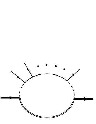
Fig. 6: One-loop $q$-$\bar{q}$-tgluon(s) diagram. The double line represents a quark. Here each solid line that constitutes the loop is a Coulomb or a tgluon.

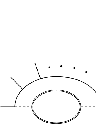
Fig. 7: Two-loop tgluon diagram. The double line represents a quark. each solid line that constitutes the loop is a Coulomb or a tgluon.

Now let us inspect Fig. 3. Cutting the line with momentum $P$ (or $Q$ or $P-Q$), we obtain an one-loop diagram. If $\omega=1$ energy divergence arises from this one-loop diagram, as has been proved in the previous section, it is cancelled out together with its relatives. Then, from Fig. 3, integrals of the forms (1.2) and (1.3) emerge, which are ill-defined ones. The integrals of the form (1.2) emerge from 1) - 3), and the integrals of the form (1.3) emerge from 3) and 4). As mentioned in Sec. I, the form (1.2) can be set equal to zero, and the integrals of the form (1.3) are connected with $V_{1}+V_{2}$ terms of Christ and Lee CL .

This is, however, not the end of the story. As a matter of fact, newcomers enter into the stage through renormalization, i.e., the renormalization counterterms. In the next section, we deal with this issue.

V Compatibility of cancellation of energy divergences and renormalizability

We adopt the minimal subtraction scheme in dimensional regularization and introduce the counter Lagrangian density $\delta{\cal L}_{\mbox{\scriptsize{eff}}}$ that includes different renormalization constants. The effective QCD Lagrangian density ${\cal L}_{\mbox{\scriptsize{eff}}}$ with addition of $\delta{\cal L}_{\mbox{\scriptsize{eff}}}$ in the strict Coulomb gauge reads nie

$${\cal L}_{\mbox{\scriptsize{eff}}}+\delta{\cal L}_{\mbox{\scriptsize{eff}}} = -\frac{Z_{31}}{2}\left(\partial_{\mu}A_{aj}\partial^{\mu}A_{a}^{j}-\partial_{i}A_{a}^{j}\partial_{j}A_{a}^{i}\right)+Z_{32}\partial_{0}A_{a}^{i}\partial_{i}A_{a}^{0}-\frac{Z_{33}}{2}\partial_{i}A_{a}^{0}\partial^{i}A_{a}^{0}$$ (5.1)

$$-\frac{1}{2\alpha}(\partial_{i}A_{a}^{i})(\partial_{j}A_{a}^{j})$$

$$+gZ_{11}f_{abc}(\partial_{i}A_{j}^{a})A_{b}^{i}A_{c}^{j}+gZ_{31}f_{abc}\partial^{0}A_{a}^{i}A_{b}^{0}A_{ci}+gZ_{32}f_{abc}\partial^{i}A^{0}_{a}A_{bi}A_{c}^{0}$$

$$-\frac{g^{2}}{4}Z_{41}f_{abc}f_{ade}A_{bi}A_{cj}A^{i}_{d}A^{j}_{e}-\frac{g^{2}}{2}Z_{31}f_{abc}f_{ade}A^{0}_{b}A_{ci}A^{0}_{d}A^{i}_{e}$$

$$+\tilde{Z}_{3}(\partial_{i}\bar{\eta}_{a})\partial^{i}\eta_{a}-gf_{abc}(\partial_{i}\bar{\eta}_{a})A_{b}^{i}\eta_{c}$$

$$+Z_{2}\bar{\psi}\left(i\partial\kern-0.44998pt\raise 1.29167pt\hbox to0.0pt{\hss/}\kern 2.5pt-(m-\delta m)\right)\psi-gZ_{1}\bar{\psi}t_{a}A_{a}^{j}\gamma_{j}\psi-gZ_{2}\bar{\psi}t_{a}A_{a}^{0}\gamma^{0}\psi\,,$$

where the limit $\alpha\to 0$ is understood to be taken. $Z$’s and $\tilde{Z}$’s in Eq. (5.1) obey the Slavnov-Taylor identities in the narrow sense,

$$\frac{Z_{31}}{Z_{11}}=\tilde{Z}_{3}=\frac{Z_{11}}{Z_{41}}=\frac{Z_{32}}{Z_{31}}=\frac{Z_{33}}{Z_{32}}=\frac{Z_{2}}{Z_{1}}\,.$$ (5.2)

The counter Lagrangian $\delta{\cal L}_{\mbox{\scriptsize{eff}}}$ introduces new vertices, which we call counter vertices. Repeating the argument in Secs. II and III on the superficial degree of energy divergence, we find that the energy divergence arises from the diagrams that are obtained from each energy-diverging diagram $G_{i}$ $(i=1,2,...)$ treated so far by inserting the counter vertices in all possible ways. Let ${\cal A}_{i}^{(j)}$ $(j=1,2,...)$ be the amplitude for thus obtained $j$th diagram, which may be computed from the Lagrangian density ${\cal L}_{\mbox{\scriptsize{eff}}}+\delta{\cal L}_{\mbox{\scriptsize{eff}}}$ in Eq. (5.1). Summing over all ${\cal A}_{i}^{(j)}$’s, we obtain ${\cal A}=\sum_{i}\left({\cal A}_{i}^{(0)}+\sum_{j}{\cal A}_{i}^{(j)}\right)$, where ${\cal A}_{i}^{(0)}$ is the amplitude for $G_{i}$.

We now show that ${\cal A}$ is free from energy divergence. Eq. (5.1) tells us that the propagators and the vertex factors extracted from ${\cal L}_{\mbox{\scriptsize{eff}}}+\delta{\cal L}_{\mbox{\scriptsize{eff}}}$ are obtained from their bare counterparts through the following replacements:

$$D^{ij}(P)\rightarrow Z_{31}^{-1}D^{ij}(P)\,,\;\;\;\;\;\;\;\;\;\;\; D^{00}(p)\rightarrow Z_{33}^{-1}D^{00}(p)\,,$$ (5.3)

$$\tilde{D}(p)\rightarrow\tilde{Z}_{3}^{-1}\tilde{D}(p)\,,\;\;\;\;\;\;\;\;\;\;\; V^{ijk}_{abc}\rightarrow Z_{11}V^{ijk}_{abc}\,,$$

$$V^{ij0}_{abc}\rightarrow Z_{31}V^{ij0}_{abc}\,,\;\;\;\;\;\;\;\;\;\;\; V^{i00}_{abc}\rightarrow Z_{32}V^{i00}_{abc}\,,$$

$$V^{ijkl}_{abcd}\rightarrow Z_{41}V^{ijkl}_{abcd}\,,\;\;\;\;\;\;\;\;\;\;\; V^{ij00}_{abcd}\rightarrow Z_{31}V^{ij00}_{abcd}\,,$$

$$\tilde{V}^{i}_{abc}\rightarrow\tilde{V}^{i}_{abc}\,.\qquad\qquad\;\,$$

where $V^{ijk}_{abc}$ is the three-tgluon vertex factor, $V^{ij0}_{abc}$ is the $A_{a}^{i}A_{b}^{j}A_{c}^{0}$-vertex factor, $\tilde{V}^{i}_{abc}$ is the $\bar{\eta}_{a}A_{b}^{i}\eta_{c}$-vertex factor, and so on. Explicit form of the quark propagator is not necessary for our purpose.

We first show that the key equations (3.4) and (3.11) remain to hold. From Eq. (LABEL:okikae), we see that ${\cal A}_{2a}$, Eq. (3.2), and ${\cal A}_{2b}^{(1)}$, Eq. (3.3), turn out to be

$${\cal A}_{2a}\longrightarrow\frac{Z_{31}^{2}}{Z_{31}}{\cal A}_{2a}=Z_{31}{\cal A}_{2a}\,,$$

and

$${\cal A}_{2b}^{(1)}\longrightarrow Z_{31}{\cal A}_{2b}^{(1)}\,,$$

respectively. Then, the same partial cancellation as for ${\cal A}_{2a}$ and ${\cal A}_{2b}^{(1)}$ in Sec. III occurs, and we obtain, in place of Eq. (3.4),

$${\cal A}_{2a}+{\cal A}_{2b}^{(1)}\longrightarrow Z_{31}\left({\cal A}_{2a}+{\cal A}_{2b}^{(1)}\right)=Z_{31}{\cal A}_{2}\,.$$ (5.4)

Taking ${\cal A}_{N}^{(G0)}$ as the reference amplitude, we have, in place of the matrices $\hat{\cal P}$ and $\hat{\cal V}$ in Eq. (3.7),

$$\hat{\cal P}=\left(\begin{array}[]{cc}-Z_{31}^{-1}Z_{33}&0\\ 0&1\end{array}\right)\,,$$

$$\hat{\cal V}=\left(\begin{array}[]{cc}0&-Z_{31}Z_{32}^{-1}/2\\ -Z_{31}Z_{32}^{-1}/2&1\end{array}\right)\,.$$

Using the identities (5.2), we have, in place of Eq. (3.9),

$$\left(\hat{\cal P}\hat{\cal V}\right)^{N}=2^{-N}\left(\begin{array}[]{cc}-N+1&N(Z_{32}/Z_{31})\\ -N(Z_{31}/Z_{32})&N+1\end{array}\right)\,.$$

Then, we see that the relation (3.10) holds as it is:

$${\cal A}_{N}^{(G)}\simeq 2^{1-N}{\cal A}_{N}^{(G0)}\,.$$

The tgluon amplitude for the FP-ghost one-loop diagrams is obtained using Eq. (LABEL:okikae),

$${\cal A}_{N}^{(FP)}=-2^{1-N}\frac{1}{\tilde{Z}_{3}^{N}}\left[\left(\frac{Z_{33}}{Z_{32}}\right)^{N}{\cal A}_{N}^{(G0)}\right]=-2^{1-N}{\cal A}_{N}^{(G0)}\,,$$

where use has been made of Eq. (5.2). Thus, ${\cal A}_{N}^{(G)}$ cancels ${\cal A}_{N}^{(FP)}$:

$${\cal A}_{N}^{(G)}+{\cal A}_{N}^{(FP)}\simeq 0\,.$$ (5.7)

Proof of Eq. (5.7) with the aid of the regularization by an interpolating gauge

The effective QCD Lagrangian density with addition of the counter Lagrangian density in the interpolating gauge, $\xi\partial_{0}A_{a}^{0}+\partial_{i}A_{a}^{i}=0$, reads

$${\cal L}_{\mbox{\scriptsize{eff}}}+\delta{\cal L}_{\mbox{\scriptsize{eff}}} = -\frac{Z_{31}}{2}\left(\partial_{\mu}A_{aj}\partial^{\mu}A_{a}^{j}-\partial_{i}A_{a}^{j}\partial_{j}A_{a}^{i}\right)+Z_{32}\partial_{0}A_{a}^{i}\partial_{i}A_{a}^{0}-\frac{Z_{33}}{2}\partial_{i}A_{a}^{0}\partial^{i}A_{a}^{0}$$ (5.8)

$$-\frac{1}{2\alpha}(\tilde{\partial}_{\mu}A_{a}^{\mu})(\tilde{\partial}_{\nu}A_{a}^{\nu})$$

$$+gZ_{11}f_{abc}(\partial_{i}A_{j}^{a})A_{b}^{i}A_{c}^{j}+gZ_{12}f_{abc}\partial^{0}A_{a}^{i}A_{b}^{0}A_{ci}+gZ_{13}f_{abc}\partial^{i}A^{0}_{a}A_{bi}A_{c}^{0}$$

$$-\frac{g^{2}}{4}Z_{41}f_{abc}f_{ade}A_{bi}A_{cj}A^{i}_{d}A^{j}_{e}-\frac{g^{2}}{2}Z_{42}f_{abc}f_{ade}A^{0}_{b}A_{ci}A^{0}_{d}A^{i}_{e}$$

$$+\tilde{Z}_{31}(\partial_{i}\bar{\eta}_{a})\partial^{i}\eta_{a}+\xi\tilde{Z}_{32}(\partial_{0}\bar{\eta}_{a})\partial^{0}\eta_{a}-gf_{abc}(\tilde{\partial}_{\mu}\bar{\eta}_{a})A_{b}^{\mu}\eta_{c}$$

$$+Z_{2}\bar{\psi}\left(i\partial\kern-0.44998pt\raise 1.29167pt\hbox to0.0pt{\hss/}\kern 2.5pt-(m-\delta m)\right)\psi-gZ_{\psi 11}\bar{\psi}t_{a}A_{a}^{j}\gamma_{j}\psi-gZ_{\psi 12}\bar{\psi}t_{a}A_{a}^{0}\gamma^{0}\psi\,,$$

where $\tilde{\partial}_{\mu}\equiv(\xi\partial_{0},\nabla)$ and $\alpha\to 0$ is understood to be taken. $Z$’s and $\tilde{Z}$’s obey

$$\frac{Z_{31}}{Z_{11}} = \tilde{Z}_{31}=\frac{Z_{11}}{Z_{41}}=\frac{Z_{32}}{Z_{12}}=\frac{Z_{33}}{Z_{13}}=\frac{Z_{2}}{Z_{\psi 11}}\,\;(\equiv D)\,,$$ (5.9)

$$\frac{Z_{31}}{Z_{12}} = \tilde{Z}_{32}=\frac{Z_{12}}{Z_{42}}=\frac{Z_{32}}{Z_{13}}=\frac{Z_{2}}{Z_{\psi 12}}\,\;(\equiv D^{\prime})\,.$$ (5.10)

These equations are derived in a similar manner as in nie . A few comments are in order.

• Diagrammatic analysis shows that $\bar{\eta}A^{\mu}\eta$ three-point function is UV finite, as it does in the Landau gauge.

• In the strict Coulomb-gauge limit, $\xi\to 0$, $D^{\prime}=1$.

Gluon- and ghost- propagators can be read off from Eq. (5.8):

$$\Delta^{ij} = \frac{1}{Z_{31}}\frac{1}{P^{2}+i0^{+}}\left[\delta^{ij}-\frac{p^{2}-2\xi(Z_{32}/Z_{33})p_{0}^{2}+\xi^{2}(Z_{31}/Z_{33})p_{0}^{2}}{(p^{2}-(Z_{31}/Z_{32})\xi p_{0}^{2}+i0^{+})^{2}}\,p^{i}p^{j}\right]\,,$$

$$= \frac{1}{Z_{31}}\frac{1}{P^{2}+i0^{+}}\left[\delta^{ij}-\frac{p^{2}-2\xi(D^{\prime}/D)p_{0}^{2}+\xi^{2}(D^{\prime}/D)^{2}p_{0}^{2}}{(p^{2}-(D^{\prime}/D)\xi p_{0}^{2}+i0^{+})^{2}}\,p^{i}p^{j}\right]\,,$$

$$\Delta^{00} = \frac{Z_{31}}{Z_{32}^{2}}\frac{p^{2}}{(p^{2}-(D^{\prime}/D)\xi p_{0}^{2}+i0^{+})^{2}}\,,$$

$$\Delta^{0i} = \Delta^{i0}=\frac{Z_{31}}{Z_{32}^{2}}\frac{\xi p_{0}p^{i}}{(p^{2}-(D^{\prime}/D)\xi p_{0}^{2}+i0^{+})^{2}}\,,$$

$$\tilde{\Delta} = \frac{1}{\xi\tilde{Z}_{32}p_{0}^{2}-\tilde{Z}_{31}p^{2}+i0^{+}}=\frac{1}{\tilde{Z}_{31}}\frac{1}{\xi(\tilde{Z}_{32}/\tilde{Z}_{31})p_{0}^{2}-p^{2}+i0^{+}}$$ (5.11)

$$= \frac{1}{\tilde{Z}_{31}}\frac{(D^{\prime}/D)\xi p_{0}^{2}-p^{2}}{(p^{2}-(D^{\prime}/D)\xi p_{0}^{2}-i0^{+})^{2}}\,,$$

where use has been made of Eqs. (5.9) and (5.10). Through the same manner as above leading to Eq. (3.21), we obtain for $\hat{\cal P}_{i}$ and $\hat{\cal V}$,

$$\hat{\cal P}_{i} = \left(\begin{array}[]{cc}(D/D^{\prime})^{2}[2(D^{\prime}/D)\tilde{p}_{i0}^{2}/p_{i}^{2}-1]&\tilde{p}_{i0}^{2}/p_{i}^{2}\\ \tilde{p}_{i0}^{2}/p_{i}^{2}&1\end{array}\right)\,,$$

$$\hat{\cal V} = \left(\begin{array}[]{cc}0&-Z_{12}/(2Z_{13})\\ -Z_{12}/(2Z_{13})&1\end{array}\right)$$

$$= \left(\begin{array}[]{cc}0&-D^{\prime}/(2D)\\ -D^{\prime}/(2D)&1\end{array}\right)\,,$$

where $\tilde{p}_{i0}=\sqrt{\xi}p_{i0}$. Matrix multiplication yields

$$\hat{\cal P}_{i}\hat{\cal V}=\frac{1}{2}\left(\begin{array}[]{cc}A_{i}-1&D/D^{\prime}\\ -D^{\prime}/D&A_{i}+1\end{array}\right)\,,$$

where

$$A_{i}=1-(D^{\prime}/D)\tilde{p}_{i0}^{2}/p_{i}^{2}\,.$$

Mathematical induction yields

$$\prod_{i=1}^{N}\left(\hat{\cal P}_{i}\hat{\cal V}\right) = \frac{1}{2^{N}}\left(\begin{array}[]{cc}\alpha_{N}^{(+)}&\beta_{N}\\ \gamma_{N}&\alpha_{N}^{(+)}\end{array}\right)\,,$$

$$\alpha_{N}^{(\pm)} = \left[\prod_{i=1}^{N}A_{i}\right]\left(1\mp\sum_{i=1}^{N}\frac{1}{A_{i}}\right)\,,$$

$$\beta_{N} = -\left(\frac{D}{D^{\prime}}\right)^{2}\gamma_{N}=\frac{D}{D^{\prime}}\left[\prod_{i=1}^{N}A_{i}\right]\sum_{i=1}^{N}\frac{1}{A_{i}}\,.$$

Then, in place of Eq. (3.23), we obtain

$${\cal A}_{N}^{(G)}\simeq\frac{2^{1-N}}{\sqrt{\xi}}\int\frac{d\tilde{p}_{0}}{2\pi}\left[\prod_{l=1}^{N}\frac{p_{l}^{2}-(D^{\prime}/D)\tilde{p}_{l0}^{2}}{p_{l}^{2}}\right]A_{N}^{(G0)}\,.$$

Using Eqs. (5.8) - (5.10) and (5.11), we obtain, in place of Eq. (3.24),

$${\cal A}_{N}^{(FP)} \simeq -\frac{2^{1-N}}{\sqrt{\xi}}\int\frac{d\tilde{p}_{0}}{2\pi}\frac{1}{\tilde{Z}_{31}^{N}}\left[\prod_{l=1}^{N}\frac{p_{l}^{2}-(D^{\prime}/D)\tilde{p}_{l0}^{2}}{p_{l}^{2}}\right]$$

$$\mbox{\hskip 43.05542pt}\times\left(\frac{Z_{33}}{Z_{13}}\right)^{N}A_{N}^{(G0)}$$

$$= -\frac{2^{1-N}}{\sqrt{\xi}}\int\frac{d\tilde{p}_{0}}{2\pi}\left[\prod_{l=1}^{N}\frac{p_{l}^{2}-(D^{\prime}/D)\tilde{p}_{l0}^{2}}{p_{l}^{2}}\right]A_{N}^{(G0)}\,.$$

Then cancellation occurs between ${\cal A}_{N}^{(G)}$ and ${\cal A}_{N}^{(FP)}$, and then, removing the regulator $\xi\to 0$, we have

$${\cal A}_{N}^{(G)}+{\cal A}_{N}^{(FP)}\simeq 0\,.$$

Thus, Eq. (5.7) gets a sound foundation.

Compatibility of cancellation of energy divergences and renormalizability

What we have shown above is that, when the renormalization counterterms are included to all orders of perturbation theory, energy-divergent contributions are cancelled out. Then, by expanding $Z$’s and $\tilde{Z}$’s in powers of $g^{2}$, energy-divergent contributions are cancelled order by order in perturbation theory.

Armed with this proposition, we are now in a position to show that the cancellation of energy divergences are compatible with the renormalizability of the theory.

We are concerned with the tgluon $N$-point one-loop amplitudes ${\cal A}_{N}$ $(N=2,3,...)$. Let ${\cal A}_{N}^{(M)}$ be the $O(g^{N+M})$ contribution to ${\cal A}_{N}$ and $G_{i}$ ($i=1,2,...$) be the set of one-loop diagrams that contributes to ${\cal A}_{N}^{(0)}$. For regularizing the energy divergence, we employ the interpolating gauge, and to handle the UV divergence we employ the dimensional regularization by continuing the spacetime dimensionality from $4$ to $d$. Then, for $\xi\neq 0$ and $d\neq 4$, all contributions to ${\cal A}_{N}$ are free from energy- and UV-divergences.

(I) $O(g^{N})$: As shown in Sec. III, ${\cal A}_{N}^{(0)}$ is free from energy divergence, i.e., finite in the limit $\xi\to 0$. For $5\leq N$, ${\cal A}_{N}^{(0)}$ is finite in the limit $d\to 4$ (UV finite). For $2\leq N\leq 4$, ${\cal A}_{N}^{(0)}$ is written in the form,

$${\cal A}_{N}^{(0)}=\frac{1}{\sqrt{\xi}}{\cal F}_{N}^{(0)}+{\cal G}_{N}^{(0)}+O(\xi^{1/2})\,.$$

Algebraic renormalizability (for arbitrary $\xi$) described above in conjunction with Eqs. (5.8) - (5.10) indicates that ${\cal F}_{N}^{(0)}$ and ${\cal G}_{N}^{(0)}$ are finite in the limit $d\to 4$ (UV finite). Furthermore, thanks to the above proof of cancellation of energy divergences, we have ${\cal F}_{N}^{(0)}=0$, so that, by removing the regulator $\xi\to 0$, we see that ${\cal A}_{N}^{(0)}$ $(={\cal G}_{N}^{(0)})$ is free from energy divergence and UV finite.

(II) $O(g^{N+2})$: Through inserting a single one-loop renormalization part into each diagram $G_{i}$ in all possible ways, we obtain a set of diagrams $G_{i}^{(j)}$ $(j=1,2,...)$. Let $\left({\cal A}_{N}^{(2)}\right)_{i}^{(j)}$ be the amplitude for $G_{i}^{(j)}$: ${\cal A}_{N}^{(2)}=\sum_{i,\,j}\left({\cal A}_{N}^{(2)}\right)_{i}^{(j)}$. As mentioned in Sec. IIIC, no overlapping energy divergence arises in $\left({\cal A}_{N}^{(2)}\right)_{i}^{(j)}$. Energy divergences and/or UV divergences that arise from one-loop subdiagrams have already been managed at the first stage (I). Then, ${\cal A}_{N}^{(2)}$ may be written in the form,

$${\cal A}_{N}^{(2)}=\frac{1}{\sqrt{\xi}}{\cal F}_{N}^{(2)}+{\cal G}_{N}^{(2)}+O(\xi^{1/2})\,.$$

The same argument as above in (I) leads ${\cal A}_{N}^{(2)}\stackrel{{\scriptstyle\xi\to 0}}{{\longrightarrow}}{\cal G}_{N}^{(2)}$ to be UV finite.

(III) Higher orders: With the aid of the Bogoliubov-Parasiuk-Hepp-Zimmerman (BPHZ) prescription bogo , one can proceed to higher orders and verify that ${\cal A}_{N}^{(M)}$ is free from energy divergence and UV finite.

Finally, it is worth mentioning that, in the course of perturbative computation, if infrared and/or mass singularities arise, we introduce small mass for gluons. It is well known that, in any reaction rate, the cancellation occur between them ln .

References

- (1) P. Doust, Ann. Phys. 177, 169 (1987).
- (2) H. Cheng and E.-C. Tsai, Phys. Lett. B176, 130 (1986); Phys. Rev. D 40, 1246 (1989).
- (3) L. Baulieu and D. Zwanziger, Nucl. Phys. B548, 572 (1999).
- (4) N. H. Christ and T. D. Lee, Phys. Rev. D 22, 939 (1980).
- (5) J. Schwinger, Phys. Rev. 127, 324 (1962).
- (6) H. Cheng and E.-C. Tsai, Phys. Rev. Lett. 57, 511 (1986).
- (7) P. J. Doust and J. C. Taylor, Phys. Lett. B197, 232 (1987).
- (8) A. Andraši and J. C. Taylor, Eur. Phys. J. C41, 377 (2005).
- (9) G. Leibbrandt and J. Williams, Nucl. Phys. B475, 469 (1996); G. Leibbrandt, ibid. B521, 383 (1998); G. Heinrich and G. Leibbrandt, ibid.B575, 359 (2000).
- (10) A. Niégawa, hep-th/0604142.
- (11) N. N. Bogoliubov and O. S. Parasiuk, Acta. Math. 97, 227 (1957); K. Hepp, Comm. Math. Phys. 2, 301 (1966); W. Zimmerman, Comm. Math. Phys. 15, 208 (1969); Lectures on Elementary Particles and Quantum Field Theory, Brandeis Summer Institute in Theoretical Physics (M.I.T. Press, Cambridge, 1970), ed. by S. Deser, M. Grisaru, and H. Pendleton. See, also, N. N. Bogoliubov, D. V. Shirkov, Introduction to the Theory of Quantized Fields, third edition, John Wiley (1980).
- (12) T. Kinoshita, J. Math. Phys. 3, 650 (1962); T. D. Lee and M. Nauenberg, Phys. Rev. 133, B1549 (1964); W. J. Marciano, Phys. Rev. D 12, 3861 (1975); G. Sterman, ibid. 14, 2123 (1976); 17, 2773, 2789 (1978); F. G. Krausz, Nucl. Phys. B126, 340 (1977); R. Akhoury, Phys. Rev. D 19, 1250 (1979); N. Ohta, Prog. Theor. Phys. 62, 1370 (1979).