BPS Condensates, Matrix Models and Emergent String Theory

Abstract:

A prescription is given for computing anomalous dimensions of single trace operators in SYM at strong coupling and large $N$ using a reduced model of matrix quantum mechanics. The method involves treating some parts of the operators as “BPS condensates” which, in certain limit, have a dual description as null geodesics on the $S^{5}$. In the gauge theory, the condensate is similar to a representative of the chiral ring and it is described by a background of commuting matrices. Excitations around these condensates correspond to excitations around this background and take the form of “string bits” which are dual to the “giant magnons” of Hofman and Maldacena. In fact, the matrix model approach gives a quantum description of these string configurations and explains why the infinite momentum limit suppresses the quantum effects. This method allows, not only to derive part of the classical sigma model Hamiltonian of the dual string (in the infinite momentum limit), but also its quantum canonical structure. Therefore, it provides an alternative method of testing the AdS/CFT correspondence without the need of integrability.

1 Introduction

Understanding the strong coupling limit of non-abelian gauge theories is still an outstanding open problem in theoretical physics. Most of our understanding comes from Conformal Field Theories (CFTs). According to the AdS/CFT conjecture, at large $N$ and large but fixed ’t Hooft coupling, we should find an effective geometrical description of these theories in terms of perturbative string theory on an asymptotically AdS background [1]. Proving (or disproving) this conjecture is still an important open problem. However, much evidence in its favor have been found in recent years. The best studied example of the correspondence is the duality between ${\cal N}=4$ SYM theory in four dimensions and string theory on $AdS_{5}\times S^{5}$. This is the model that we will study in this paper.

The most significant obstruction to proving the correspondence is our inability to make strong coupling calculations in SYM theory. Pure supersymmetric states have protected dimensions and so one can map them directly to SUGRA excitations on the dual string theory. However, for non-supersymmetric states one needs to be more clever and find a way to extrapolate a weak coupling calculation to strong coupling. As in any perturbative expansion, the secret is to be careful in choosing the “background” state one is expanding around.

It was realized a few years ago that one can define the perturbation theory around the supersymmetric single trace 1/2 BPS states of the form

$$\hbox{ Tr}(Z^{J})\;,$$ (1)

with $Z$ one of the three complex adjoint scalars of SYM. For large $J$ these states are dual to point-like classical strings rotating with angular momentum $J$ along a null geodesic on the equator of the $S^{5}$. The first “small” non-BPS excitations to be understood where the so-called BMN states of the form [3]

$$\sum_{l}e^{ipl}\hbox{ Tr}(Z^{J-l}XZ^{l}X)\;,$$ (2)

where $p\sim 1/J$.

In fact, the effective geometry seen by the small strings is a plane wave and thus it allows the exact calculation of the spectrum in the string theory side. It turns out that for these fast rotating strings the expansion parameter in their energy is of the form $\sim\lambda/J^{2}$. It is then possible to extrapolate a perturbative calculation in SYM by first taking $J$ large and then $\lambda\rightarrow\infty$ but with $\lambda/J^{2}=\text{fixed}\ll 1$.

On the string theory side, however, the limit is the opposite: $\lambda\gg 1$ first to get perturbative string theory, and then focus on trajectories with $J\gg 1$. Surprisingly, both calculations agree up to order $\lambda^{3}$ where a $1/J$ discrepancy is has been found [4]. It is believed that the discrepancy is just an artifact of the opposite order of limits and the fact that keeping $\lambda/J^{2}$ fixed entangles both $1/\sqrt{\lambda}$ and $1/J$ quantum corrections.

One can proceed along these lines and consider states with many transverse “impurities”, e.g.

$$\hbox{ Tr}(ZXXZX\cdots)\;.$$ (3)

One can compute the anomalous dimension matrix in this basis and it has been found that one can also define large charge limits with $J_{X},J_{Z}\rightarrow\infty$ that allow to extrapolate the weak coupling calculation to strong coupling. On the string theory dual one find that these states correspond to long semiclassical rotating strings. As before, one considers a limit where $\lambda/J^{2}$ is held fixed. One can even match the sigma model actions for these strings in this limit [6, 7, 8], but one again finds a discrepancy at three loops [9].

One can also define an expansion around BPS D-brane states called Giant Gravitons. The limits described above are also useful for this case and one can show agreement with the string theory at one loop [10, 11].

It is apparent at this point that all of the comparisons described above require certain amount of confidence in extrapolating the weak coupling results in SYM to strong coupling. One would like to be able to define a strong coupling expansion directly. This is of course the “holy grail” of high energy physics. In any case, it is believed that this expansion is possible at least in SYM based on integrability.

In the last years there has been great hope that integrability will allow to prove AdS/CFT at least in the free closed string sector. This hope was motivated by the discovery of integrability at one loop in the gauge theory dilatation operator [12] and was followed by the discovery of classical integrability in the string theory world-sheet [13].

The quantum integrability in the gauge theory has been argued to persist at higher loops and an all-loop guess for the Bethe ansatz has been presented in [14, 15]. This has also been accompanied by a similar guess for the presumed quantum Bethe ansatz for the dual string theory [16]. The all loop Bethe ansatz for the gauge theory was actually used in the higher loop test of AdS/CFT described above.

One can see that the proposed integrable structures are very similar on both sides of the correspondence but they do not quite agree. In fact, all the disagreement can be encoded in a single overall phase in the Bethe ansatz’ $S$-matrix [16]. Solving this discrepancy is still an open problem. In any case, using integrability to prove/test AdS/CFT has some major drawbacks. First, integrable structures are very delicate and can fail at higher loop as it happens in the plane wave matrix model [17]. Failure of integrability at two loops has also been claimed to happen for the open strings on Giant Gravitons [19, 20]. This is specially concerning since all of the test of AdS/CFT so far rely on an (educated) guess at higher loops. In fact, the quantum integrability of the string theory is still a conjecture. Secondly, even if integrability works for ${\cal N}=4$ SYM it will not work for other less symmetric CFTs.

It is then very desirable to develop techniques that allow a systematic large $\lambda$ expansion directly from the gauge theory without the need of integrability. We believe that the key for this program lies again in expanding around highly supersymmetric states. Moreover, given the general combinatorial nature of the dilatation operator in terms of spin chains (at least for the scalar sector), it seems very likely that one can always find a reduced quantum mechanical model to describe the effective dynamics of certain sectors of the theory. In fact this idea was originally put forward by Berenstein in [21]. It was argued there that the effective dynamics of 1/2 BPS states can be described by a reduced quantum mechanical model of a single matrix in an harmonic oscillator potential which, after diagonalization, can be written as $N$ fermions in an harmonic trap. One can describe semiclassical states of the theory in terms of droplets in the single particle phase space. Reduced quantum mechanical sectors are also known to arise in thermal ${\cal N}=4$ SYM on $\mathbb{R}\times S^{3}$ [22, 23].

For the 1/2 BPS states, the reduced model was amazingly confirmed by a SUGRA calculation in [24], where it was found that all the 1/2 BPS solutions in IIB SUGRA can also be classified in terms of droplets in a plane.

Generalizations of the reduced matrix model for 1/4 and 1/8 BPS states were proposed in [25] in terms of multiple matrix models of commuting matrices. The gravity side of the story for these states is still incomplete, but some recent progress has been made in [26]. Nevertheless, some important consistency checks for the proposal in [25] have been put forward recently. First, the ground state for the 1/8 BPS model is described by a singular distribution of eigenvalues on an $S^{5}\subset\mathbb{R}^{6}$ in the large $N$ limit [25]. One can calculate quadratic excitations around this background of commuting matrices and one finds that they can be pictured as “string bits” which joint two eigenvalues on the sphere. The spectrum of these excitations has a dispersion relation [27],

$$E(p)=\sqrt{1+\frac{\lambda}{\pi^{2}}\sin^{2}(p/2)}=\sqrt{1+\frac{\lambda}{\pi^{2}}\sin^{2}(\Delta\varphi/2)}\;,$$ (4)

where $p$ is the momentum of the BMN state (2) and $\Delta\varphi$ is the azimuthal angle between the two eigenvalues on the sphere. This is in fact the exact proposed dispersion relation in the Bethe ansatz of both the gauge theory and the string dual [14, 15, 16].

What is more surprising is that the picture of the “string bits” and the relation $p=\Delta\varphi$ was recently confirmed by Hofman and Maldacena using a purely classical string theory analysis [32]. These authors introduced a limit where one takes $J\rightarrow\infty$ with $p$ fixed. It was proposed that the “magnon” excitations of the form (2) are dual to classical string solutions on $S^{2}$ that form a straight line joining two points on the boundary of the circular droplet (the equator of $S^{2}$ in the usual coordinates). These “giant magnons” have a dispersion relation like (4) (at large $\lambda$) after identifying $p=\Delta\varphi$. This confirms the prediction of the matrix model calculation! Moreover, these matrix model techniques can also be applied to more general CFTs as in [30, 31].

Therefore, even though we do not have a proof that the effective dynamics of scalar operators is given by a reduced matrix model, we have non-trivial checks that this is indeed the case.

In this article we attempt to clarify the meaning of the matrix model calculations. In particular we give a precise proposal that relates the matrix model computations to the more familiar operator mixing problem. This is done in terms of what we call “BPS condensates” which are summarized in section 2. A detailed discussion is given in sections 3 and 4 where we also review how one obtains the giant magnons of [32] directly from the matrix model calculation and how one can generalize these to the $SU(3)$ sector of the theory. For the $SU(3)$ sector, however, the matching with the dual string theory is more restricted since it turns out that one needs to understand the backreaction to the 1/4 and 1/8 BPS condensates.

In any case, we obtain a quantum description of the giant magnons and we get a better understanding of why the Hofman-Maldacena limit is really a classical limit. The possible interpretation of magnon bound states in our formalism is briefly discussed in section 3. We also show how the matrix model calculation gives not only the correct Hamiltonian for the string states (in the infinite momentum limit) but also the canonical structure expected from the string theory dual. This is very encouraging since it would be very desirable to match directly the sigma model of the string theory and its canonical structure rather than having to solve for its spectrum. This would allow generalizations to other less symmetric field theories. In section 5 we discuss the backreaction to the BPS condensates and we explain why our method works in the strong coupling limit. Finally we discuss the prospects to relate this procedure to the more familiar Bethe Ansatz technique on the conclusion.

2 The General Idea of BPS Condensates

Here we want to summarize the general idea of BPS condensates using the familiar single trace scalar operators of SYM theory. In the next sections we will develop the details of this method and its interpretation in terms of the dual string theory.

When doing perturbative calculations in either the gauge theory or the string dual one always has to choose a classical background configuration to expand upon. In the gauge theory side of the correspondence one can rephrase this as defining the expansion around certain set of operators that are dual to classical string configurations as we discussed in the introduction.

Here we want to rephrase this expansion in terms of the effective matrix model mentioned above. Lets start by considering a generic $SU(2)$ single trace operator. One can write this kind of state using the bosonized language introduced in [10, 11]:

$$\hbox{ Tr}(YZ^{n_{1}}YZ^{n_{2}}Y\cdots)\;.$$ (5)

In the next section we argue that these states are described by a quantum mechanical matrix model of two complex matrices. For large $n_{i}$ one can see the $Y$s as impurities in an otherwise 1/2 BPS operator $\hbox{ Tr}(Z^{n})$. In the excited state (5), the $Z^{n_{i}}$s look localy like BPS states and we call them 1/2 BPS condensates. In the matrix model it then makes sense to expand around a background of normal matrices: $[Z,\bar{Z}]=0$ and $Y=0$. This “classical” BPS background can be the circular droplet for example and we identify it with the 1/2 BPS condensate in the operator language. The fluctuations $\delta Y$ are called “string bits” and they are dual to commutators between the $Y$ and the BPS condensates in the operator language:

$$\hbox{ Tr}(Z^{n})\rightarrow\hbox{ Tr}([Y,Z^{n_{1}}][Y,Z^{n_{2}}]\cdots)\;,\;\;\;\sum_{i}n_{i}=n\;.$$ (6)

The states (5) serve as a basis for these excitations. The fluctuation $\delta Z$ are the backreaction of the condensate and in this case we will see that they can be integrated out to give an effective action for the transverse excitations on the classical BPS background.

In the dual string theory we will see that for $n_{i}\rightarrow\infty$ the 1/2 BPS condensates become classical and localize the ends of the string bits on the boundary of the circular droplet. Namely, a null geodesic on $\mathbb{R}\times S^{1}$. This is precisely the interpretation advocated recently in [32]. This will be discussed in detail in the next section.

If the number of $Y$ fields is comparable to the number of $Z$s, it makes sense to expand around a state of the form:

$$\hbox{ Tr}(\{Z^{n}Y^{m}\})\;.$$ (7)

Here the curly brackets denote symmetrization between the letters $Y$ and $Z$. This state is just a rotation of the 1/2 BPS state. For multi-trace operators, symmetrized states similar to this one are 1/4 BPS [33, 34]. Small excitations around this state will be described by turning on commutators that break the symmetrization,

$$\hbox{ Tr}(\{Z^{n}Y^{m}\})\rightarrow\hbox{ Tr}([Y,\{Z^{n_{1}}Y^{m_{1}}\}][Z,\{Z^{n_{2}}Y^{m_{2}}\}]\cdots)\;,\;\;\text{etc.}$$ (8)

One can find a basis for these excitations in analogy to (5),

$$\hbox{ Tr}(Y\{Z^{n_{1}}Y^{m_{1}}\}Z\{Z^{n_{2}}Y^{m_{2}}\}\cdots)\;.$$ (9)

Since the words $\{Z^{n_{i}}Y^{m_{i}}\}$ look like 1/4 BPS states we call them 1/4 BPS condensates. As in the case of the 1/2 BPS condensates this description is more useful when $n_{i},m_{i}\rightarrow\infty$. As we will see, the dual interpretation is that, in this limit, the 1/4 BPS condensates localize the ends of the string bits on null geodesic on $\mathbb{R}\times S^{3}$.

In the matrix model language we should then expand around a “classical” configuration of commuting normal matrices $[Y,Z]=0=[Z,\bar{Z}]=[Y,\bar{Y}]=0$. This configuration can be one of the 1/4 “droplets” of [25]. For the ground state we get a $S^{3}$ distribution of eigenvalues. The fluctuations around this background will correspond to the commutators:

$$\delta Z\simeq[Z,\{Z^{n_{i}}Y^{m_{i}}\}]\;,\;\;\;\delta Y\simeq[Y,\{Z^{n_{i}}Y^{m_{i}}\}]\;.$$ (10)

We discuss these fluctuations in section 4.

The generalization to $SU(3)$ states should be obvious by now. For example, in the case where we have many $Y$ and $Z$ fields and a few $X$s, we can consider the following basis for the transverse excitations

$$\hbox{ Tr}(X\{Z^{n_{1}}Y^{m_{1}}\}X\{Z^{n_{2}}Y^{m_{2}}\}\cdots)\;.$$ (11)

In the matrix model we expand around $[Y,Z]=[Y,\bar{Y}]=[Z,\bar{Z}]=0$, $X=0$. In this case a fluctuation $\delta Y$ or $\delta Z$ amounts to a breaking one the condensates and thus leaving this restricted basis, e.g.

$$\{Z^{n_{i}}Y^{m_{i}}\}\rightarrow[Z,\{Z^{n_{i}-1}Y^{m_{i}}\}]\;.$$ (12)

On the other hand, a $\delta X$ fluctuation is just a commutator between an $X$ and one of the condensates.

We can now try to consider states with many $Z$s (for example) and similar quantities of $Y$ and $X$. In this case it make sense to expand in a basis like

$$\hbox{ Tr}(XZ^{n_{1}}YZ^{n_{2}}\cdots)\;.$$ (13)

In the matrix model we diagonalize $Z$ and expand around $[Z,\bar{Z}]=0$, $X=Y=0$ just like in the $SU(2)$ case.

Finally we can have 1/8 BPS condensates by considering symmetrized combinations $\{X^{n_{i}}Y^{m_{i}}Z^{p_{i}}\}$. In this case we expand around configurations with three normal commuting matrices. The fluctuations are dual to the commutators between any of the fields and the condensates just like for the $SU(2)$ states.

3 1/2 BPS Condensates: The $SU(2)$ Sector

In this section we briefly review the 1/2 BPS states and their effective dynamics in terms of a normal matrix model. We then consider generic $SU(2)$ states an set up an effective description in terms of a two matrix model similar to the one in [27]. We then construct the Hilbert space in terms of the 1/2 BPS condensates. We obtain the canonical commutator relations for these states and explain how to obtain their classical limit. In doing so, we recover the picture of the “string bits” of [25, 11] and explain its precise relation with the “giant magnons” of [32]. Moreover, we match the canonical structure expected from the dual string theory and also its sigma model in the limit of large $\lambda$ and infinite angular momentum. Finally, we comment on the a possible interpretation of the bound states of [32, 35, 36, 37] in terms of the matrix model.

3.1 Review of 1/2 BPS States Dynamics

The 1/2 BPS states of SYM theory are described by multitrace operator build out of a single complex scalar: ${\cal O}_{n_{1}n_{2}\cdots}=\hbox{ Tr}(Z^{n_{1}})\hbox{ Tr}(Z^{n_{2}})\cdots$ (see [41] and references therein). They are eigenstates of the dilatation operator with dimension

$$\hat{\Gamma}|{\cal O}_{n_{1}n_{2}\cdots}{\rangle}=(n_{1}+n_{2}+\ldots)|{\cal O}_{n_{1}n_{2}\cdots}{\rangle}=\hat{J}_{z}|{\cal O}_{n_{1}n_{2}\cdots}{\rangle}\;.$$ (14)

It is well known that at one loop, the contribution from the D-term in the scalar potential $V_{D}\sim\hbox{ Tr}|[Z,\bar{Z}]|^{2}$ to the dilatation operator is canceled by fermion and gauge loops [42]. One can translate this to the dual Hilbert space as,

$${\langle}{\cal O}_{n_{1}n_{2}\cdots}|\hbox{ Tr}|[Z,\bar{Z}]|^{2}|{\cal O}_{n_{1}^{\prime}n_{2}^{\prime}\cdots}{\rangle}=0\;.$$ (15)

Since these states are protected by supersymmetry, we expect this to be true independently of the gauge coupling.

From Eqs. (14) and (15) it is natural to guess that the effective dynamics of these states will be described by a normal gauged matrix model with an harmonic oscillator potential [21, 41, 43, 44],

$$S=\int dt\hbox{ Tr}(|D_{t}Z|^{2}+|Z|^{2})\;,\;\;\;\;[Z,\bar{Z}]=0\;.$$ (16)

This model can be visualized as a reduction of SYM on $\mathbb{R}\times S^{3}$ down to the zero mode of a single scalar [25, 21]. The eigenstates of the matrix model can be expressed as antisymmetric wave function of the complex eigenvalues $z_{i}$ and can be classified in terms of Young Tableux [21]. Their quantum numbers match (14).

Moreover, in the large $N$ limit generic coherent states are described by “droplet”-like distributions of eigenvalues on the complex plane. For example, the ground state $\psi_{0}\sim e^{-\hbox{ Tr}(Z\bar{Z})}$ will have a probability density,

$${\langle}\psi_{0}|\psi_{0}{\rangle}=\int_{[Z,\bar{Z}]=0}[dZd\bar{Z}]|\psi_{0}|^{2}\propto\int\prod_{i=1}^{N}d^{2}z_{i}\,\,e^{-2\sum_{i}|z_{i}|^{2}+\sum_{i<j}\log|z_{i}-z_{j}|^{2}}\;,$$ (17)

which will be dominated by the saddle point of the exponential in the large $N$ limit. Here we have used the measure change for a normal matrix model which follows from the metric $ds^{2}=\hbox{ Tr}(dZd\bar{Z})$ [45].

In the limit $N\rightarrow\infty$ one replaces the sums by density distributions and one extremizes the functional

$$E[\rho]=-2\int d^{2}z\rho(z)|z|^{2}+\frac{1}{2}\int\int d^{2}z_{1}d^{2}z_{2}\rho(z_{1})\rho(z_{2})\log|z_{1}-z_{2}|^{2}\;\;,$$ (18)

with the constraint $N=\int d^{2}z\rho(z)$. Using the fact that the logarithm is the Green’s function in two dimensions one obtains a circular droplet distribution of eigenvalues of constant density given by [45]

$$\sigma=-\frac{\Delta W(z,\bar{z})}{4\pi}=-\frac{\partial\bar{\partial}W(z,\bar{z})}{\pi}=\frac{2}{\pi}\;,$$ (19)

where $W(z,\bar{z})=-2|z|^{2}$ is the potential for the eigenvalues. Then, from the normalization of the density one obtains the radius of the droplet: $r_{0}=\sqrt{N/2}$. The droplet approximation is very useful for calculating correlation functions in position space as we will see below.

We would like to comment that there is a possible second matrix model that gives the same description of the 1/2 BPS states. This is a complex matrix model with the action (16). It turns out that one can transform $Z$ as $Z\rightarrow U^{\dagger}(Z_{\text{diag}}+R)U$, where $U\in SU(N)$, $Z_{\text{diag}}$ is diagonal and $R$ is strictly upper triangular [45]. The measure change is [45],

$$[dZd\bar{Z}]\propto\prod_{i=1}^{N}d^{2}z_{i}\prod_{j<k}|z_{j}-z_{k}|^{2}\prod_{m<n}d^{2}R_{mn}\;.$$ (20)

One can easily see that the ground state wave function will be the same as in the normal matrix model and that for holomorphic correlation functions, the matrix $R$ does not contribute [45]. Therefore, the dynamics of this model (in the holomorphic sector) is the same as with a normal matrix. However, as we will see, the distinction can be important for multiple matrix models.

3.2 $SU(2)$ States Dynamics

A generic $SU(2)$ operator has the form:

$$\hbox{ Tr}(ZYZZ\cdots)\hbox{ Tr}(ZYYZ\cdots)\cdots\;.$$ (21)

For these holomorphic states one still has that the D-term contributions add to zero at one loop. Therefore, we expect that we can also ignore the D-terms from the effective matrix model. The lack of supersymmetry can make this model much more complicated that the 1/2 BPS case. However one can argue along the lines of [25] that for the 1/4 BPS states the corresponding matrix model is a simple rotation of (16):

$$S_{\text{1}/4BPS}=\sum_{\alpha=Y,Z}\hbox{ Tr}\left(|D_{t}Z_{\alpha}|^{2}+|Z_{\alpha}|^{2}\right)\;,$$ (22)

for normal commuting matrices $[Z_{\alpha},Z_{\beta}]=[Z_{\alpha},\bar{Z}_{\alpha}]=0$.

At one loop, the anomalous dimension is again generated by the commutators from the F-terms: $\hbox{ Tr}|[Z_{\alpha},Z_{\beta}]|^{2}$. We can again argue for an all-loop generalization [27] involving two complex matrices and ignoring the D-terms:

$$S=\int dt\hbox{ Tr}\left[\sum_{\alpha}(|D_{t}Z_{\alpha}|^{2}+|Z_{\alpha}|^{2})+\frac{g_{YM}^{2}}{(2\pi)^{2}}\sum_{\alpha,\beta}|[Z_{\alpha},Z_{\beta}]|^{2}+\text{higher commutators}\right]\;.$$ (23)

The first three terms of the action come from the direct reduction of SYM on the $S^{3}$ to the zero mode of the matrices, and the higher commutators will come from integrating out higher modes and fields. A similar matrix model arises from the one-loop dilatation operator in the $SU(2)$ sector [28, 29].

As in any quantum system one chooses a particular classical configuration for which to define the perturbation theory. To define a consistent perturbative expansion one needs to find stable classical configurations. In our case, we know that in the large $N$ limit (and with $Y=0$) the normal matrix model $[Z,\bar{Z}]=0$ can be described by droplets on the single particle phase space of the eigenvalues of $Z$. Moreover, these configurations are stabilized by SUSY. It then makes sense to expand around these “classical” solutions. Since the classicality is only statistical, one needs a prescription to define this expansion. We do this in the following way. First write as usual $Z\rightarrow Z+\delta Z$, and we diagonalize the background $Z$. Then, we treat the eigenvalues $z_{i}$ as random numbers with probability distribution $\sim\exp(-2\sum_{i}|z_{i}|^{2}+\sum_{i<j}\log|z_{i}-z_{j}|^{2})$. The resulting operators and states of the Hilbert space will depend on $z_{i}$. Therefore, we define the inner product to be the statistical average of the usual one:

$${\langle}\phi|\hat{\cal O}|\tilde{\phi}{\rangle}\equiv\frac{\int\prod_{i}d^{2}z_{i}|\psi_{0}(\{z_{i}\})|^{2}{\langle}\phi(\{z_{i}\})|\hat{\cal O}(\{z_{i}\})|\tilde{\phi}(\{z_{i}\}){\rangle}}{\int\prod_{i}d^{2}z_{i}|\psi_{0}(\{z_{i}\})|^{2}}\;.$$ (24)

In the large $N$ limit we can use the saddle point approximation as before.

We now need to take into account the backreaction to 1/2 BPS background, $\delta Z$. If we ignore the possible higher commutators in the action (23), we see that the fluctuation $\delta Z$ enters quadratically in the action and can be integrated out leaving an effective action for the matrix $Y$ in the BPS background $Z$. This will result in higher interactions for $Y$. In this article we will ignore these interactions for simplicity. These higher interactions are suppressed in the strong coupling and infinite momentum limit as we discuss below.

At this point, our procedure is pretty much equivalent to the one in [46, 47], but the approach presented here is simpler and allows generalizations beyond the $SU(2)$ sector as we will see in the next sections. Matrix models in terms of collective fields describing the BMN limit of SYM have also been studied in [48, 49].

Finally, one also has the possibility of expanding around the ground state of the complex matrix model mentioned in the previous section. It turns out that the distinction between the two backgrounds goes to zero in the infinite momentum limit discussed in the next section.

3.3 1/2 BPS Condensates, String Bits and Giant Magnons

We can now calculate the effective hamiltonian for the $Y$ fields on the background of $Z$. After diagonalizing the normal matrix $Z$, we have,

$$H=\sum_{i,j}\omega_{ij}\left[(A^{\dagger}_{Y})_{i}^{j}(A_{Y})^{i}_{j}+(A^{\dagger}_{\bar{Y}})_{i}^{j}(A_{\bar{Y}})^{i}_{j}\right]+\text{interactions}\;,$$ (25)

where the creation operators are given by

$$(A_{Y}^{\dagger})_{i}^{j} = \sqrt{\frac{w_{ij}}{2}}[Y_{i}^{j}-\frac{i}{\sqrt{w_{ij}}}(\pi_{Y})_{i}^{j}]\;,$$ (26)

$$(A_{\bar{Y}}^{\dagger})_{i}^{j} = \sqrt{\frac{w_{ij}}{2}}[\bar{Y}_{i}^{j}-\frac{i}{\sqrt{w_{ij}}}(\pi_{\bar{Y}})_{i}^{j}]\;,$$ (27)

with

$$\omega_{ij}=\sqrt{1+\frac{\lambda}{(2\pi)^{2}}|z_{i}-z_{j}|^{2}}\;.$$ (28)

Here we have assumed that the fermions cancel the zero-point energy from normal ordering the operators in (25). Finally, we have normalized the diagonal matrix so that $z_{i}=r_{i}e^{i\phi_{i}}$ with $r_{i}\leq 1$.

We can now construct the Hilbert space of states. With our normalization a generic single trace state takes the form

$$|n_{1},n_{2},\ldots,n_{L}{\rangle}=\frac{1}{N^{L/2}}\hbox{ Tr}(A_{Y}^{\dagger}\psi_{n_{1}}(Z)A_{Y}^{\dagger}\psi_{n_{2}}(Z)\cdots A_{Y}^{\dagger}\psi_{n_{L}}(Z))|0{\rangle}_{Y}\;,$$ (29)

where,

$$\psi_{n}(Z)=\sqrt{1+n}Z^{n}\;,$$ (30)

and $|0{\rangle}_{Y}$ is the usual vacuum for $Y$ defined by $A_{Y}|0{\rangle}_{Y}=A_{\bar{Y}}|0{\rangle}_{Y}=0$. The wavefunctions $\psi_{n}(Z)$ are dual to the 1/2 BPS condensates. In fact as we will see they will localize on an $S^{1}$ at large $n$ just like the 1/2 BPS states. This is the infinite momentum limit. The $A_{Y}^{\dagger}$ excitations are called “string bits” [25, 27] and as we will see they have a dual description as the “giant magnons” of [32].

It is easy to verify the orthonormality of these states using our inner product prescription:

$${\langle}n_{1},n_{2},\ldots,n_{L}|n_{1}^{\prime},n_{2}^{\prime},\ldots,n_{L}^{\prime}{\rangle}\approx\prod_{l=1}^{L}\int[dD_{l}]\psi_{n_{l}}(z_{l})^{*}\psi_{n_{l}^{\prime}}(z_{l})=\prod_{l=1}^{L}\delta_{n_{l},n_{l}^{\prime}}\;,$$ (31)

where $\int[dD]=\int_{0}^{1}drr\int_{0}^{2\pi}d\phi/\pi$ is the integration across the droplet, and we are assuming the generic case where not all of the $n_{i}$ are equal so we ignore the cyclicity of the trace.

Now lets consider calculating the expectation value of some observable, say the Hamiltonian (25). After doing the usual planar contractions of the $A_{Y}$s one can always reduce the problem to a product of integrals over the droplet. A useful property of the 1/2 BPS condensates is

$$Z\psi_{n}(Z)=\sqrt{\frac{n+1}{n+2}}\psi_{n+1}(Z)\;.$$ (32)

Under the inner product (70) one then sees that $Z$ and $\bar{Z}$ can be treated as the operators $\hat{Z}^{\dagger}$ and $\hat{Z}$ with the property:

$$\hat{Z}^{\dagger}|n{\rangle} = \sqrt{\frac{n+1}{n+2}}|n+1{\rangle}\equiv\hat{r}e^{i\hat{\phi}}|n{\rangle}$$ (33)

$$\hat{Z}|n{\rangle} = \sqrt{\frac{n}{n+1}}|n-1{\rangle}\equiv e^{-i\hat{\phi}}\hat{r}|n{\rangle}\;,$$ (34)

where we define

$$\hat{r}=\sqrt{\frac{\hat{n}}{\hat{n}+1}}\;,\;\;\;e^{i\hat{\phi}}|n{\rangle}=|n+1{\rangle}\;.$$ (36)

Note that ${\langle}\hat{r}{\rangle}\leq 1$ and thus as the notation suggests, this will become the operator that measures the radial distance of the droplet. We also observe that $\hat{n}$ is the momentum conjugate to $\hat{\phi}$, $[\hat{\phi},\hat{n}]=i$, or in terms of $\hat{r}$, $\hat{p}_{\phi}=\hat{r}^{2}/(1-\hat{r}^{2})$. From the canonical commutator relation we can derive,

$$[\hat{\phi},\hat{r}]=i\frac{(1-\hat{r}^{2})^{2}}{2\hat{r}}\;.$$ (37)

This indicates that our system is constrained, which is not surprising since we are restricting our Hilbert space by choosing these special $SU(2)$ states. As we will see, this is exactly the expected canonical structure for the $SU(2)$ states in the string theory dual after an appropriate gauge choice.

It is easy to show that for any function $f(Z,\bar{Z})$ with a power law expansion,

$$\int[dD]\psi_{n}(z)^{*}f(z,\bar{z})\psi_{n^{\prime}}(z)\cong{\langle}n|{{}^{\circ}_{\circ}}f(\hat{Z}^{\dagger},\hat{Z}){{}^{\circ}_{\circ}}|n^{\prime}{\rangle}\;,$$ (38)

where ${{}^{\circ}_{\circ}}{{}^{\circ}_{\circ}}$ denotes anti-normal ordering with respect to the operators $\hat{Z}^{\dagger}$, $\hat{Z}$. Therefore, we can write the quadratic Hamiltonian in our basis as

$$H^{(2)}=\sum_{l=1}^{L}{{}^{\circ}_{\circ}}\sqrt{1+\frac{\lambda}{(2\pi)^{2}}|\hat{Z}^{\dagger}_{l}-\hat{Z}^{\dagger}_{l+1}|^{2}}\;{{}^{\circ}_{\circ}}\;.$$ (39)

Let us now discuss the possibility of expanding around the background corresponding to the ground state of the complex matrix model discussed in the previous section. Ignoring again the backreaction, we regard the matrix $Z$ as a random variable with distribution $\int[dZd\bar{Z}]\exp(-2\hbox{ Tr}(Z\bar{Z}))$. Now consider the Hamiltonian at one-loop in $\lambda$. The anomalous dimension will be generated by a term $\propto\hbox{ Tr}[Z,A_{Y}^{\dagger}][\bar{Z},A_{Y}]$.

Lets apply this to the state $|\psi{\rangle}\sim\hbox{ Tr}(\cdots Z^{n_{1}}A_{Y}^{\dagger}Z^{n_{2}}\cdots)$. It is easy to see that the anomalous dimension Hamiltonian will act in such a way to introduce a $Z$ and $\bar{Z}$ fields at the left and right of $A_{Y}^{\dagger}$ so that we conserve the $U(1)$ charge. As an example, consider the interaction that takes $Z^{n_{1}}\rightarrow Z^{n_{1}}\bar{Z}Z$. Then, the matrix elements for this kind of interactions will be reduced to the following correlation function,

$$\frac{{\langle}\hbox{ Tr}(\bar{Z}^{n_{1}^{\prime}}Z^{n_{1}}\bar{Z}Z){\rangle}}{\sqrt{{\langle}\hbox{ Tr}(\bar{Z}^{n_{1}^{\prime}}Z^{n_{1}^{\prime}}){\rangle}\hbox{ Tr}(\bar{Z}^{n_{1}}Z^{n_{1}}){\rangle}}}\approx\frac{N}{2}\delta_{n_{1},n_{1}^{\prime}}\;,$$ (40)

where we have taken the planar limit.

Now consider doing the same correlation function but with the normal matrix model (NMM),

$$\frac{{\langle}\hbox{ Tr}(\bar{Z}^{n_{1}^{\prime}}Z^{n_{1}}\bar{Z}Z){\rangle}_{\text{NMM}}}{\sqrt{{\langle}\hbox{ Tr}(\bar{Z}^{n_{1}^{\prime}}Z^{n_{1}^{\prime}}){\rangle}_{\text{NMM}}{\langle}\hbox{ Tr}(\bar{Z}^{n_{1}}Z^{n_{1}}){\rangle}_{\text{NMM}}}}\approx\frac{\int[dD]\bar{z}^{n_{1}^{\prime}+1}z^{n_{1}+1}}{\int[dD]|z|^{2n_{1}}}=\frac{N}{2}\left(\frac{n_{1}+1}{n_{1}+2}\right)\delta_{n_{1},n_{1}^{\prime}}\;.$$ (41)

We see that both results agree only in the infinite spin limit $n_{1}\rightarrow\infty$.

Therefore, we can regard the calculations done in this paper with a normal matrix background as asymptotic in the large spin limit. In any case, we can calculate corrections to this limit with the backreaction term $\delta Z$. We leave these calculations for the interested reader.

3.4 Classical Limit and the dual String Theory

In Quantum Mechanics one usually recovers the classical limit by taking $\hbar\rightarrow 0$. This makes the canonical commutators vanish, $[x,p]=i\hbar\rightarrow 0$ so that $x$ and $p$ become simple classical observables. For constrained systems the classical limit can be trickier. In our case we can see from (37) that the classical limit is reached by taking states for which ${\langle}\hat{r}{\rangle}\rightarrow 1$, or ${\langle}\hat{n}{\rangle}\rightarrow\infty$. This is precisely the localization on the edge of the droplet which is correlated to the limit where the $Y$ impurities are “far away”. This limit also takes away the ordering ambiguities from the Hamiltonian which becomes

$$H^{(2)}\approx\sum_{l=1}^{L}\frac{\sqrt{\lambda}}{\pi}\sin\left(\frac{\phi_{l}-\phi_{l+1}}{2}\right)\;,$$ (42)

where we have taken the large $\lambda$ limit to compare with the string theory.

This is precisely the Hamiltonian of the “giant magnons” of [32]. In fact, the whole picture is exactly the same: we can picture the $Y_{i}^{j}$ as an excitation (string bit) joining two eigenvalues $z_{i}$ and $z_{j}$ which become localized at the edge of the droplet when $n\rightarrow\infty$. In fact, taking $n\rightarrow\infty$ with $\Delta\phi$ fixed is precisely the Hoffman-Maldacena limit. Here, however, we have a full quantum description of the system. One can see that finite $n$ effects will delocalize the ends of the string bits and make them “fuzzy” on the $S^{2}$ (fig. 1).

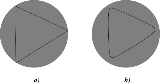
Figure 1: In figure a) we show the usual giant magnons at infinite momenta $n_{i}\rightarrow\infty$. The lines are identified with the “string bits” $Y_{i}^{j}$ and the edges with the 1/2 BPS condensates $Z^{n_{i}}$. Here the disk is mapped to an $S^{2}\subset S^{5}$ so that the edge is the equator of the $S^{2}$. Finite $n_{i}$ effects will delocalize the ends of the magnons away from the equator as shown in figure b).

Finite $n$ effects were considered recently in [50] for a single giant magnon. Their results confirm that the ends of the giant magnon are delocalized from the equator at finite $n$.

The relation between the momentum of the magnons and the angles on the droplet can be seen more clearly by Fourier transforming as in [27]. For example, consider the following asymptotic state,

$$|\psi(p){\rangle}=\lim_{\Delta\rightarrow\infty}\lim_{n\rightarrow\infty}\sum_{x=-\Delta}^{\Delta}e^{ipx}\hbox{ Tr}(\cdots Y^{\dagger}Z^{n+x}Y^{\dagger}Z^{n-x}Y^{\dagger}\cdots)|0{\rangle}_{\text{Y}}\;,$$ (43)

where we first take the limit of infinite separation $n\rightarrow\infty$. One can show that these states are approximately orthogonal in this limit.

For condensates of infinite angular momentum the operators (33) and (34) become simple shift generators,

$$\hat{Z}|n{\rangle}\approx|n-1{\rangle}\;,\;\;\;\hat{Z}^{\dagger}|n{\rangle}\approx|n+1{\rangle}\;.$$ (44)

Focusing on a single string bit, the effective Hamiltonian between these asymptotic states is simply,

$$H^{(2)}_{l,l+1}\approx\sqrt{1+\frac{\lambda}{(2\pi)^{2}}{\cal H}_{l,l+1}}\;,$$ (45)

where,

$${\cal H}_{l,l+1}|n_{l},n_{l+1}{\rangle}=2|n_{l},n_{l+1}{\rangle}-|n_{l}-1,n_{l}+1{\rangle}-|n_{l}+1,n_{l+1}-1{\rangle}\;.$$ (46)

This is the same asymptotic Hamiltonian found in the two matrix model of [47]. The eigenstates of this Hamiltonian are simply plane waves of the form (43) with energy,

$$E_{\text{asymp.}}=\sqrt{1+\frac{\lambda}{\pi^{2}}\sin^{2}\left(\frac{p}{2}\right)}\;.$$ (47)

Comparing with (42) we see that $p\cong\Delta\phi$.

We can also match the canonical structure of these string bits to the one found in the string theory side. Since these are $SU(2)$ states they must be a limit of the well known rotating strings on $\mathbb{R}\times S^{3}$ [5]. A well known limit of these strings is the one corresponding to “long strings”: $L\rightarrow\infty$ with $\lambda/L^{2}=\text{fixed}\ll 1$ as discussed in the introduction. The canonical structure should not depend on the particular limit we are taking since $L$ is a conserved quantum number. One can calculate the Polyakov action for these string using the following coordinates on the $S^{3}$ [11]:

$$Z=re^{i(t+\phi)}\;,\;\;Y=\sqrt{1-r^{2}}e^{i\varphi}\;.$$ (48)

One then chooses the gauge, $\tau=t$, $p_{\varphi}=\text{const.}$, which is appropriate to compare with the bosonized labeling of the states (29). One obtains the action,

$$S\approx L\int dt\int_{0}^{1}d\sigma\left[\frac{r^{2}\dot{\phi}}{1-r^{2}}-1-\frac{\lambda}{8\pi^{2}L^{2}}(r^{\prime 2}+r^{2}\phi^{\prime 2})+{\cal O}\left(\frac{\lambda^{2}}{L^{4}}\right)\right]\;,$$ (49)

where one eliminates the time derivatives of all the higher order terms [7, 8] and,

$$L=\sqrt{\lambda}\int_{0}^{1}d\sigma p_{\varphi}\;,\;\;\;\lambda=g_{YM}^{2}N=R^{4}/\alpha^{\prime 2}\;.$$ (50)

The same action can be found from the spin chain formalism in the gauge theory at one loop using the coherent states for the Cuntz algebra [11]. From this action we see that the canonical momenta are

$$p_{r}=0\;,\;\;\;p_{\phi}=L\frac{r^{2}}{1-r^{2}}\;.$$ (51)

This are precisely the constraints found above from the matrix model calculation!

The additional factor of $L$ comes from taking the large $L$ limit, since the total momentum for the $Z$ fields in the gauge theory becomes:

$$\hat{J}_{Z}=\sum_{l=1}^{L}\hat{n}_{l}\approx L\int_{0}^{1}d\sigma\frac{\hat{r}^{2}}{1-\hat{r}^{2}}\;.$$ (52)

One can also reproduce the commutator algebra by using the classical Dirac brackets for constrained systems [51]. The Dirac bracket is defined by

$$\{A,B\}_{\text{D}}=\{A,B\}_{\text{PB}}-\sum_{i,j}\{A,f_{i}\}_{\text{PB}}(G^{-1})_{ij}\{f_{j},B\}_{\text{PB}}\;,$$ (53)

where $\{,\}_{\text{PB}}$ is the usual Poisson bracket. Furthermore, the second class constraints are given by the equations $f_{i}=0$ and $G^{-1}$ is the inverse of

$$G_{ij}=\{f_{i},f_{j}\}_{\text{PB}}\;.$$ (54)

The constraints are given by:

$$f_{1}=p_{r}\;,\;\;\;f_{2}=p_{\phi}-L\frac{r^{2}}{1-r^{2}}\;.$$ (55)

Then it is straightforward to verify

$$\{\phi,r\}_{\text{D}}=\frac{(1-r^{2})^{2}}{2Lr}\;.$$ (56)

The comparison with the quantum theory is done as usual: $[,]=i\{,\}_{\text{class.}}$. One then obtains precisely the continuum version of the commutators (37).

3.5 Multiple Giant Magnons and Bound States

Suppose that we put many string bits together as in the state (5). One of two things can happen: either we have the trivial addition of classical giant magnons, or we form a bound state. The first outcome happens if we take the formal $n_{i}\rightarrow\infty$ limit for each condensate. The total energy in the limit of many string bits ($L\gg 1$) is,

$$H^{(2)}\approx\sum_{l=1}^{L}\frac{\sqrt{\lambda}}{\pi}\sin\left(\frac{\phi_{l}-\phi_{l+1}}{2}\right)\approx\frac{\sqrt{\lambda}}{2\pi}\int_{0}^{1}d\sigma\partial_{\sigma}\phi=\frac{\sqrt{\lambda}}{2\pi}\Delta\phi\;.$$ (57)

Here we assume that $L$ does not scale in any way with $\lambda$. If we scale $L$ as in the fast string limit, $\lambda/L^{2}\ll 1$ we get instead,

$$H^{(2)}\approx L\int_{0}^{1}d\sigma\left(1+\frac{\lambda}{8\pi^{2}L^{2}}\phi^{\prime 2}+\cdots\right)\;.$$ (58)

This agrees with the classical string action (49) at one loop.

Understanding the emergence of bound states and of strings at $r<1$, requires taking into account $1/n_{i}$ corrections. However, there are two effects that can be important for understanding these corrections. First, as we discussed above we need to take into account the backreaction term in the matrix model. Furthermore, one needs to understand the possible higher order interactions that can come from integrating higher spherical harmonics in SYM. We do not have a good understanding of these issues at this moment. However, suppose that these unknown interactions tend to normal order the Hamiltonian (39). Then one can deduce the classical limit by constructing coherent states for the operators $\hat{Z}_{l}$.

In fact, one can show that the states,

$$|z{\rangle}=(1-|z|^{2})\sum_{n=0}^{\infty}\sqrt{n+1}z^{n}|n{\rangle}\;,$$ (59)

are indeed overcomplete coherent states of the operator $\hat{Z}$. The completeness relation is,

$$\int_{0}^{1}\frac{drr}{(1-r^{2})^{2}}\int_{0}^{2\pi}\frac{d\phi}{\pi}|z{\rangle}{\langle}z|=1\;.$$ (60)

The classical Hamiltonian in the coherent state basis will be,

$${\langle}:H^{(2)}:{\rangle}=\sum_{l=1}^{L}\sqrt{1+\frac{\lambda}{(2\pi)^{2}}|Z_{l}-Z_{l+1}|^{2}}\approx\frac{\sqrt{\lambda}}{2\pi}\int_{0}^{1}\sqrt{r^{\prime 2}+r^{2}\phi^{\prime 2}}\;,$$ (61)

where in the last step we have taken the strong coupling limit and then the continuum limit corresponding to a large number of string bits. This is exactly the Nambu-Goto action for a string on $\mathbb{R}\times S^{2}$ in the static gauge [32].

Of course, the presence of bound states follows directly from the duality between this action and the Sine-Gordon theory [32]. These bound states and its generalizations have been studied recently in [35, 36, 37, 38, 39, 40].

4 1/4 and 1/8 BPS Condensates: The $SU(3)$ Sector

The concept of 1/4 BPS condensates was discussed briefly in section 2. Here we will study these condensates in detail as we did for the 1/2 BPS case. The general states we want to consider are of the form

$$\hbox{ Tr}(X\{Z^{n_{1}}Y^{m_{1}}\}Y\{Z^{n_{2}}Y^{m_{2}}\}Z\cdots)\;.$$ (62)

In particular we are interested in the limit where $n_{i},m_{i}\rightarrow\infty$ with the number of “impurities” outside of the condensates held fixed.

By the same arguments of the previous section, we expect an effective description of generic $SU(3)$ states in terms of a matrix model similar to (23) but now with three complex matrices ($\alpha=X,Y,Z$). There are two complications in the $SU(3)$ case, however. The fluctuations $\delta X$, $\delta Y$ and $\delta Z$ cannot be integrated out so easily. This is actually a good thing as these fluctuations have an interpretation in the operator language as we discussed in section 2.

Moreover, it turns out that we need to include the D-terms to the action. This conclusion follows from comparing with the string theory results (see below). We do not have a purely field theoretical explanation for this but it seems to be a consequence of the fact that we have less supersymmetry for these states and hence the one loop result is not protected at strong coupling. The effective action for these states is then of the form,

$$S = \int dt\hbox{ Tr}\left[\sum_{\alpha}(|D_{t}Z_{\alpha}|^{2}+|Z_{\alpha}|^{2})+\frac{g_{YM}^{2}}{(2\pi)^{2}}\sum_{\alpha,\beta}|[Z_{\alpha},Z_{\beta}]|^{2}\right.$$ (63)

$$\left.+\frac{g_{YM}^{2}}{(2\pi)^{2}}\sum_{\alpha,\beta}|[Z_{\alpha},\bar{Z}_{\beta}]|^{2}+\text{higher commutators}\right]\;.$$

As we discussed in section 2, for large $n_{i},m_{i}$ the states (62) look like many “condensates” of 1/4 BPS operators involving $Z$ and $Y$ fields. Therefore we can try to define our expansion around “classical” configurations with $[Z,Y]=[Z,\bar{Z}]=[Y,\bar{Y}]=0$. The classical configurations will be the eigenstates of the 1/4 BPS action (22) in the large $N$ limit. In particular, we know that the ground state is given by $\psi_{0}\sim e^{-\hbox{ Tr}(|Z|^{2}+|Y|^{2})}$ [25]. Thus, the energy functional that determines the geometry of the eigenvalue distribution is

$$E[\rho]=-2\int d^{4}x\rho(x)(|z|^{2}+|y|^{2})+\frac{1}{2}\int\int d^{4}x_{1}d^{4}x_{2}\rho(x_{1})\rho(x_{2})\log(|y_{1}-y_{2}|^{2}+|z_{1}-z_{2}|^{2})\;,$$ (64)

where we have used the measure change for two normal commuting matrices:

$$[dZd\bar{Z}dYd\bar{Y}]\propto\prod_{i}d^{2}z_{i}d^{2}y_{i}\prod_{k<l}(|y_{k}-y_{l}|^{2}+|z_{k}-z_{l}|^{2})\;.$$ (65)

Doing a saddle point calculation as in [27] one finds that the eigenvalues form a singular distribution on an $S^{3}\subset\mathbb{R}^{4}$ with radius $r_{0}=\sqrt{N}/2$. The fluctuations around this background are the non-BPS parts of these operators.

The motivation for this interpretation is the same as with the 1/2 BPS condensates. If we consider calculating the one loop anomalous dimension for these states we see that the planar contribution from the F-term and D-term commutators $\hbox{ Tr}|[Z,Y]|^{2}$, $\hbox{ Tr}|[Z,\bar{Y}]|^{2}$ will be zero when contracted between the condensates. Only contractions between fields outside the condensates and the condensates themselves will give rise to anomalous dimensions. We interpret these interactions as fluctuations around the commuting background. The interactions $\hbox{ Tr}|[Z,X]|^{2}$, $\hbox{ Tr}|[Z,\bar{X}]|^{2}$ and $\hbox{ Tr}|[Y,X]|^{2}$, $\hbox{ Tr}|[Y,\bar{X}]|^{2}$ that involve a condensate and a transverse $X$ field are interpreted as the fluctuation $\delta X$ in the matrix model. Finally the interactions $\hbox{ Tr}|[Z,Y]|^{2}$, $\hbox{ Tr}|[Z,\bar{Y}]|^{2}$ with $Z$ or $Y$ fields outside the condensate are just the backreaction of the condensate $\delta Y$ and $\delta Z$.

4.1 Hilbert Space and Canonical Structure

To simplify the discussion let us start with the states

$$\hbox{ Tr}(X\{Z^{n_{1}}Y^{m_{1}}\}X\{Z^{n_{2}}Y^{m_{2}}\}X\cdots)\;.$$ (66)

That is, let us ignore the backreaction to the 1/4 BPS condensates for the moment ($\delta Y=\delta Z=0$). We then diagonalize the classical background of commuting normal matrices. The effective Hamiltonian for the $X$ fluctuations will have the same form as for the $SU(2)$ case (25) but now with the following dispersion relation

$$\omega_{ij}=\sqrt{1+\frac{\lambda}{(2\pi)^{2}}\left(|y_{i}-y_{j}|^{2}+|z_{i}-z_{j}|^{2}\right)}\;.$$ (67)

Note that if we had ignored the D-terms, the dispersion relation would have an additional factor of 1/2: $\sqrt{1+\frac{\lambda}{2(2\pi)^{2}}(|\Delta z|^{2}+|\Delta y|^{2})}$.

In analogy with the 1/2 BPS condensates, the basis for this sector is

$$|n_{1},m_{1};n_{2},m_{2};\ldots;n_{L},m_{L}{\rangle}=\frac{1}{N^{L/2}}\hbox{ Tr}[A_{X}^{\dagger}\psi_{n_{1},m_{1}}(Y,Z)\cdots A_{X}^{\dagger}\psi_{n_{L},m_{L}}(Y,Z)]|0{\rangle}_{X}\;,$$ (68)

with

$$\psi_{n,m}(Y,Z)=\sqrt{\frac{(n+m+1)!}{n!m!}}Z^{n}Y^{m}\;.$$ (69)

Using the saddle point approximation, the inner product can be reduced to integrals over an $S^{3}$ in the large $N$ limit:

$${\langle}n_{1},m_{1};\ldots;n_{L},m_{L}|n_{1}^{\prime},m_{1}^{\prime};\ldots;n_{L}^{\prime},m_{L}^{\prime}{\rangle} \approx \prod_{l=1}^{L}\int\frac{(d\Omega_{3})_{l}}{\text{Vol}(S^{3})}\psi_{n_{l},m_{l}}(y_{l},z_{l})^{*}\psi_{n_{l}^{\prime},m_{l}^{\prime}}(y_{l},z_{l})$$ (70)

$$= \prod_{l=1}^{L}\delta_{n_{l},n_{l}^{\prime}}\delta_{m_{l},m_{l}^{\prime}}\;,$$

where $z,y$ become coordinates on the three-sphere, $|y|^{2}+|z|^{2}=1$.

Just like in the $SU(2)$ sector, we can treat $Z$ and $Y$ as creation operators under our inner product. They obey the following properties:

$$\hat{Z}^{\dagger}|\psi_{n,m}{\rangle} = \sqrt{\frac{n+1}{2+n+m}}|\psi_{n+1,m}{\rangle}\equiv\frac{\hat{r}_{1}}{\sqrt{1+\hat{\eta}}}e^{i\hat{\phi}_{1}}|\psi_{n,m}{\rangle}\;,$$ (71)

$$\hat{Y}^{\dagger}|\psi_{n,m}{\rangle} = \sqrt{\frac{m+1}{2+n+m}}|\psi_{n,m+1}{\rangle}\equiv\frac{\hat{r}_{2}}{\sqrt{1+\hat{\eta}}}e^{i\hat{\phi}_{2}}|\psi_{n,m}{\rangle}\;,$$ (72)

$$e^{i\hat{\phi}_{1}}|\psi_{n,m}{\rangle} = |\psi_{n+1,m}{\rangle}\;,$$ (73)

$$e^{i\hat{\phi}_{2}}|\psi_{n,m}{\rangle} = |\psi_{n,m+1}{\rangle}\;,$$ (74)

$$\hat{r}_{1} = \sqrt{\frac{\hat{n}}{\hat{n}+\hat{m}}}\;,$$ (75)

$$\hat{r}_{2} = \sqrt{\frac{\hat{m}}{\hat{n}+\hat{m}}}\;,$$ (76)

$$\hat{r}_{1}^{2}+\hat{r}_{2}^{2} = 1\;,$$ (77)

$$\hat{\eta} = \frac{1}{\hat{n}+\hat{m}}\;.$$ (78)

We can now calculate the following canonical structure:

$$[\hat{\phi}_{1},\hat{r}_{1}] = i\frac{\hat{r}_{2}^{2}}{2\hat{r}_{1}}\hat{\eta}\;,$$ (79)

$${[}\hat{\phi}_{1},\hat{r}_{2}{]} = -i\frac{\hat{r}_{2}}{2}\hat{\eta}\;,$$ (80)

$${[}\hat{\eta},\hat{\phi}_{\alpha}{]} = i\hat{\eta}^{2}\;,$$ (81)

and the conjugate momentum to $\hat{\phi}_{\alpha}$ is $\hat{P}_{\alpha}=\hat{r}_{\alpha}^{2}/\hat{\eta}=\hat{n}_{\alpha}$.

One can also show that the operators are antinormal ordered under the inner product (see Appendix A) and so the effective quadratic Hamiltonian is just

$$H^{(2)}=\sum_{l=1}^{L}{{}^{\circ}_{\circ}}\sqrt{1+\frac{\lambda}{(2\pi)^{2}}\left(|\hat{Y}^{\dagger}_{l}-\hat{Y}^{\dagger}_{l+1}|^{2}+|\hat{Z}^{\dagger}_{l}-\hat{Z}^{\dagger}_{l+1}|^{2}\right)}\;{{}^{\circ}_{\circ}}\;.$$ (82)

4.2 Localization and the Classical Limit

The localization of the 1/4 BPS condensates works just like for the 1/2 BPS case. Looking at the canonical commutators (71) we see that for states with ${\langle}\hat{n}+\hat{m}{\rangle}\rightarrow\infty$ with ${\langle}\hat{n}{\rangle}/{\langle}\hat{m}{\rangle}$ fixed will localize on an $S^{3}$. The operators $\hat{r}_{\alpha}$, $\hat{\phi}_{\alpha}$ become commuting (classical) numbers and we can drop the anti-normal ordering symbols on the Hamiltonian (82) and replace the operators by classical coordinates on the $S^{3}$, $|Y_{l}|^{2}+|Z_{l}|^{2}=1$.

In the case of the 1/2 BPS condensates, the localization occurs from $S^{2}\rightarrow S^{1}$. The form of the commutators (71) suggests that for the 1/4 BPS case the localization occurs as $S^{4}\rightarrow S^{3}$. We will confirm this intuition by comparing with the dual string states. But first lets try to match the canonical structure as we did with the 1/2 BPS condensates.

It is now important to remind the reader that the canonical structure found in the string theory side is sensitive to 1) the string configurations that we are considering and 2) the gauge choice in the sigma model action. One could think that since the states (66) are a restricted subset of the $SU(3)$ sector (ignoring backreaction) one will not be able to match the canonical structure found in the gauge theory side. However this is not correct since we can always expand around these states and, if we take into account the backreaction to the 1/4 BPS condensates, we have a complete basis of states for this sector. Thus in this case the particular canonical structure is tied to the choice of basis and therefore, in the string theory side, it will be related to the gauge choice in the sigma model. We would have obtained a different canonical structure had we expanded around 1/8 BPS condensates which are of the form $\hbox{ Tr}(\{X^{n}Y^{m}Z^{p}\}\cdots)$ for example (see below).

We can now find the sigma model action for the $SU(3)$ sector in the “fast string” limit: $J_{X}\rightarrow\infty$, $\lambda/J_{X}^{2}=\text{fixed}$, just like we did in the $SU(2)$ sector. The form of the operators (66) tells us that the correct gauge choice is the one that distributes the angular momentum in $X$ uniformly along the string. Looking at the commutators (71) one realizes that a convenient spacetime coordinate system for these strings is,

$$Z=\frac{r_{1}}{\sqrt{1+\eta}}e^{i(t+\phi_{1})}\;,\;\;\;Y=\frac{r_{2}}{\sqrt{1+\eta}}e^{i(t+\phi_{2})}\;,\;\;\;X=\sqrt{\frac{\eta}{1+\eta}}e^{i\varphi}\;,$$ (83)

where $r_{1}^{2}+r_{2}^{2}=1$. We now choose the gauge

$$t=\tau\;,\;\;\;p_{\varphi}=\text{const.}$$ (84)

Following the standard procedure of eliminating time derivatives for spatial derivatives [7, 8] in the sigma model one finds (see Appendix B),

$$S = L\int d\tau\int_{0}^{1}d\sigma\left[\frac{r_{1}^{2}}{\eta}\dot{\phi_{1}}+\frac{r_{2}^{2}}{\eta}\dot{\phi_{2}}\right.$$ (85)

$$\left.-1-\frac{\lambda\,\eta}{2(4\pi)^{2}L^{2}(1+\eta)^{2}}\left(\frac{\eta^{\prime 2}}{4\eta}+\sum_{\alpha=1,2}(r_{\alpha}^{\prime 2}+r_{\alpha}^{2}\phi_{\alpha}^{\prime 2})\right)+{\cal O}\left(\frac{\lambda^{2}}{L^{4}}\right)\right]\;.$$

We see that the canonical structure is exactly as in the matrix model calculation: $p_{\phi_{\alpha}}\sim r_{\alpha}^{2}/\eta$ with the other momenta set to zero. In fact, one can confirm the continuum version of the commutators (79) - (81) by using the Dirac brackets with the following constraints:

$$f_{1}=r_{1}^{2}+r_{2}^{2}-1\;,\;\;f_{2}=p_{r_{1}}\;,\;\;f_{3}=p_{r_{2}}\;,\;\;f_{5}=p_{\phi_{1}}-Lr_{1}^{2}/\eta\;,\;\;f_{6}=p_{\phi_{2}}-Lr_{2}^{2}/\eta\;.$$ (86)

The localization on the $S^{3}$ can be understood in the same way as with the 1/2 BPS condensates: it correspond to the classical limit $\eta\rightarrow 0$.

Note however, that unlike in the $SU(2)$ sector, the classical Hamiltonian that follows from the action (85) does not match with the naive classical limit of the matrix model Hamiltonian (82) at one loop. This is indeed not surprising since we are ignoring the backreaction to the condensates which is unavoidable in the $SU(3)$ sector. We will come back to this point in section 5.

4.3 $SU(3)$ Giant Magnons?

A natural question to ask at this point is whether we can match the matrix model Hamiltonian (82) at finite $L$ with some sort of $SU(3)$ giant magnon solution in the string theory side. In general one would expect that in the limit $n_{l}+m_{l}\rightarrow\infty$ each $X$ string bit would correspond to a giant magnon configuration connecting two null geodesics of the form,

$$Z=r_{1}e^{it}\;,\;\;Y=r_{2}e^{it}\;,\;\;r_{1}^{2}+r_{2}^{2}=1\;,$$ (87)

one for each condensate to the left and right of the string bit.

Note however that these 1/4 BPS condensates do not correspond to the Giant Magnons with multiple angular momenta studied recently in the literature [38, 39, 40] which represent bound states in the operator language.

The states (66) are very restricted if we ignore the backreaction to the condensates. Therefore, we can only expect a matching for some very special configurations. In particular one intuitively expects that configurations for which the ends of the giant magnon are at different radii $r_{\alpha}$ are unstable and thus would require the understanding of the backreaction since on the dual gauge theory, one would have $Z$ and $Y$ fields flowing from one condensate to the next. We should then consider configurations for which $r_{\alpha}$ is the same at each site. In the dual string theory this would correspond to giant magnons connecting the same null trajectory.

The classical limit of the energy formula (82) for these special states is,

$$E_{\text{string bit}}=\frac{\sqrt{\lambda}}{\pi}\sqrt{r_{1}^{2}\sin^{2}\left(\frac{\Delta\phi_{1}}{2}\right)+r_{2}^{2}\sin^{2}\left(\frac{\Delta\phi_{2}}{2}\right)}\;.$$ (88)

It turns out that with our simple ansatz for the classical string (see below), the matching with this quadratic formula only works for a subset of these states: those with $\Delta\phi_{1}=\Delta\phi_{2}$. These can be considered as “rotations” of the usual $SU(2)$ giant magnons. This restricted matching is hardly surprising since only in this case the spacetime probed by the string is actually flat. More generally, the backreaction to the string bit should take into account the curvature of the sphere and correct the naive square root form (88).

Let us now turn our attention to the classical string theory. We will consider strings moving on $\mathbb{R}\times S^{4}$ but for simplicity we restrict the motion on the $S^{3}\subset S^{4}$ as follows:

$$Z=r_{1}\sin[\psi(\sigma)]e^{i(\tau+\phi_{1}(\sigma))}\;,\;\;Y=r_{2}\sin[\psi(\sigma)]e^{i(\tau+\phi_{2}(\sigma))}\;,\;\;X=\cos[\psi(\sigma)]\;.$$ (89)

After defining new coordinates $\phi_{1}=\phi_{+}+\phi_{-}$ and $\phi_{2}=\phi_{+}-\phi_{-}$, the Nambu-Goto action in the static gauge $t=\tau$ becomes,

$$S_{\text{NG}}=\frac{\sqrt{\lambda}}{2\pi}\int d\tau d\phi_{+}\sqrt{x^{\prime 2}+x^{2}\ \left[1+2a\phi_{-}^{\prime}+\phi_{-}^{\prime 2}(1-bx^{2})\right]}\;,$$ (90)

where $x=\sin\psi$, $a=r_{1}^{2}-r_{2}^{2}$, $b=4r_{1}^{2}r_{2}^{2}$ and the derivative is with respect to $\phi_{+}$. The equations of motion are,

$$\phi_{-}^{\prime} = \frac{\alpha G-ax^{2}}{x^{2}(1-bx^{2})}\;,$$ (91)

$$u(x)G\frac{d}{dx}\left(\frac{u(x)}{G}\right) = x\left[1+a\phi_{-}^{\prime}+\phi_{-}^{\prime 2}(1-2bx^{2})\right]\;,$$ (92)

where

$$G=x\sqrt{\frac{a^{2}x^{2}-(u^{2}+x^{2})(1-bx^{2})}{\alpha^{2}-x^{2}(1-bx^{2})}}\;,$$ (93)

$u=dx/d\phi_{+}$ and $\alpha$ is an integration constant. Therefore we can reduce the problem to a non-linear ODE for $u(x)$ .

Let us now consider the special case of $r_{1}=r_{2}=1/\sqrt{2}$. One can easily show that the reality of $G$ implies that $\alpha=0$ and so $\phi_{-}^{\prime}=0$. The equations of motion reduce exactly to the ones for the $SU(2)$ giant magnon. The energy is [32],

$$E|_{r_{1}=r_{2}}=\frac{\sqrt{\lambda}}{\pi}\left|\sin\left(\frac{\Delta\phi_{+}}{2}\right)\right|\;,$$ (94)

where $\Delta\phi_{1}=\Delta\phi_{2}=\Delta\phi_{+}$.

One can also show that setting $\alpha=0$ implies $r_{1}=r_{2}=1/\sqrt{2}$. This follows from the reality of $u(x)$. Setting $\alpha=0$ and integrating the resulting equations of motion gives

$$u(x)=|b|\frac{x^{2}(1-x^{2})}{1-bx^{2}}\sqrt{\frac{1-bx_{\text{min}}^{2}}{x_{\text{min}}^{2}(1-x_{\text{min}}^{2})}-\frac{1-bx^{2}}{x^{2}(1-x^{2})}}\;,$$ (95)

where $x_{\text{min}}$ is the turning point. At the boundary $x=1$, the reality of $u(x)$ requires $b=1$ which in turn implies $r_{1}=r_{2}=1/\sqrt{2}$.

Now lets study the solutions with $\alpha\neq 0$. For these strings, the equation of motion for $u(x)$ is highly complicated. However it turns out that it has a very simple solution: the Giant Magnon of [32]. To see this, we first note that the boundary condition $u(x=1)$ is actually determined by the EOM. When we set $x=1$ in (92) all dependence on $u^{\prime}(x)$ drops and one is left with an equation for $u(1)$:

$$u(1)=\frac{1}{\alpha}\sqrt{a^{2}-\alpha^{2}}\;,$$ (96)

where we need $\text{sign}(\alpha)=\text{sign}(a)$, and $a^{2}\geq\alpha^{2}$. This last inequality also follows from the reality of $G$ at the boundary $x=1$.

We can now relate this to the Giant Magnon solution in [32] for which,

$$u(x)=\frac{x^{2}}{x_{\text{min}}}\sqrt{1-\left(\frac{x_{\text{min}}}{x}\right)^{2}}\;.$$ (97)

Comparing (97) with (96) we find that $\alpha=ax_{\text{min}}$. With $\alpha$ now determined by the turning point $x_{\text{min}}$ we can easily check that (97) satisfies (92). Therefore, as pointed out before, the solutions that we have found are just rotations of the Giant Magnon of [32]. Nevertheless they are consistent with the interpretation in terms of 1/4 BPS condensates. This is because the ends of the Giant Magnon travel along null geodesics in $S^{3}$ which carry two angular momenta corresponding to the two fields $Z$ and $Y$ in the condensate, which is itself a rotation of the 1/2 BPS condensate.

The generalization to 1/8 BPS condensates should be obvious by now. These will be of the form $\hbox{ Tr}(\{X^{n}Y^{m}Z^{p}\}\cdots)$ but since there are no transverse excitations left, the inclusion of the backreaction is unavoidable. The eigenvalue distribution turns into a singular $S^{5}\subset\mathbb{R}^{6}$ with radius $r_{0}=\sqrt{N}/2$. In this case it is perhaps more useful to use a $SO(6)$ invariant notation as in [27]. In this case, the dispersion relation in any direction $a=1,\ldots,6$ is,

$$w^{a}_{ij}=\sqrt{1+\frac{\lambda}{(2\pi)^{2}}|\vec{x}_{i}-\vec{x}_{j}|^{2}}\;,$$ (98)

where $\vec{x}_{i}^{2}=1$ are the coordinates in the $S^{5}$.

5 Backreaction to BPS Condensates

To simplify the discussion we can look at the 1/4 BPS condensates of the $SU(2)$ sector. That is consider operators of the form

$$\hbox{ Tr}(Y\{Z^{n_{1}}Y^{m_{1}}\}Z\{Z^{n_{2}}Y^{m_{2}}\}\cdots)\;.$$ (99)

This way we can work with the simpler matrix model (23). The proposal is that we consider expanding around the “classical” configuration of commuting matrices $[Y,Z]=[Z,\bar{Z}]=[Y,\bar{Y}]=0$ in the action (23) as we did for the $SU(3)$ sector. Then the two possible excitations $Y$ and $Z$ outside the condensates will be described by the backreaction terms $\delta Y$ and $\delta Z$ in the matrix model.

In this case it is difficult to make comparisons with the string theory dual because, as we will see, the number of excitations outside the condensates is not conserved. We can, however try to match the qualitative picture we expect from a formal field theory calculation using the operators (99). In the limit, $n_{i},m_{i}\rightarrow\infty$ we again expect that the “impurities” outside the condensates will not interact with each other. On the other hand, we expect only interactions between impurities and the condensates. First, lets consider the quadratic fluctuation around the commuting background.

Expanding $Z_{\alpha}\rightarrow Z_{\alpha}+Y_{\alpha}$ where $Z_{\alpha}$ is the commuting background, one finds the following quadratic Hamiltonian (after diagonalizing the background)

$$H^{(2)}=\sum_{i,j}(\pi_{\alpha})_{i}^{j}(\bar{\pi}_{\alpha})_{j}^{i}+M^{\alpha\beta}_{ij}(Y_{\alpha})_{i}^{j}(\bar{Y}_{\beta})_{j}^{i}\;,$$ (100)

where,

$$M^{\alpha\beta}_{ij}=\left(\begin{array}[]{cc}1+\alpha|z_{ij}|^{2}&-\alpha z_{ij}\bar{y}_{ij}\\ -\alpha\bar{z}_{ij}y_{ij}&1+\alpha|y_{ij}|^{2}\\ \end{array}\right)$$ (101)

and $\alpha=\lambda/(2\pi)^{2}$, $z_{ij}=z_{i}-z_{j}$ and similarly for $y$.

Naively one might think that the mass matrix can be diagonalized. However, we need to be very careful with the gauge invariance of the states. Diagonalizing the mass matrix means that we make a change of basis that depend on the background. On the other hand, any change of basis must be of the form,

$$(Y_{\alpha})_{i}^{j}=\sum_{\beta}f^{\beta}_{ij}(\phi_{\beta})_{i}^{j}\;,$$ (102)

where $\phi_{\beta}$ are the (normalized vectors) that diagonalize the mass matrix and, by gauge invariance, $f^{\beta}_{ij}$ must only depend on positive powers of $z_{ij}$ and $y_{ij}$ (and their conjugates). Diagonalizing the mass matrix one finds the following eigenvectors and corresponding masses:

$$(\phi_{1})_{i}^{j} = \frac{1}{\sqrt{|z_{ij}|^{2}+|y_{ij}|^{2}}}\left(\begin{array}[]{c}z_{ij}\\ -y_{ij}\\ \end{array}\right)\;,\;\;\;M_{1}^{2}=1+\alpha(|z_{ij}|^{2}+|y_{ij}|^{2})$$ (105)

$$(\phi_{2})_{i}^{j} = \frac{1}{\sqrt{|z_{ij}|^{2}+|y_{ij}|^{2}}}\left(\begin{array}[]{c}\bar{y}_{ij}\\ \bar{z}_{ij}\\ \end{array}\right)\;,\;\;\;M_{2}^{2}=1$$ (108)

Inverting these relations one finds for example,

$$(Y_{1})_{i}^{j}=\frac{1}{\sqrt{|z_{ij}|^{2}+|y_{ij}|^{2}}}(\bar{z}_{ij}(\phi_{1})_{i}^{j}+y_{ij}(\phi_{2})_{i}^{j})\;,$$ (109)

which is not allowed by gauge invariance. Even if we try to avoid this by not normalizing the eigenvectors one always runs into an ill defined square root at some point of the procedure (when defining the oscillator operators). This is telling us that $H^{(2)}$ is really an interacting Hamiltonian.

Using the usual oscillator basis we find $H^{(2)}=H^{(2)}_{0}+H^{(2)}_{\text{i}nt}$, where

$$H_{0}^{(2)} = w_{ij}^{\alpha}(A_{\alpha}^{\dagger})_{i}^{j}(A_{\alpha})_{j}^{i}\;,$$ (110)

$$H_{\text{i}nt}^{(2)} = -\frac{\alpha z_{ij}\bar{y}_{ij}}{2\sqrt{w_{ij}^{y}w_{ij}^{z}}}(A^{\dagger}_{y})_{i}^{j}(A_{z})_{j}^{i}+h.c.\;,$$ (111)

where $w_{ij}^{y}=\sqrt{1+\alpha|z_{ij}|^{2}}$ etc. and we are taking expectation values on holomorphic states. Therefore, we observe that the interaction term represents the process of interchanging an “impurity” outside the condensate with one of the fields of the condensate (with opposite polarization):

$$\hbox{ Tr}(\cdots Z\{Z^{n}Y^{m}\}\cdots)\leftrightarrow\hbox{ Tr}(\cdots Y\{Z^{n+1}Y^{m-1}\}\cdots)\;.$$ (112)

There are also cubic and quartic interactions. Lets consider the cubic ones. These do not preserve the number of impurities. On holomorphic states these interactions take the following form:

$$H^{(3)}=\frac{\alpha z_{ij}}{r_{0}}(\tilde{A}_{Y}^{\dagger})_{i}^{j}[\tilde{A}_{Y},\tilde{A}_{Z}]_{j}^{i}+\frac{\alpha y_{ij}}{r_{0}}(\tilde{A}_{Z}^{\dagger})_{i}^{j}[\tilde{A}_{Z},\tilde{A}_{Z}]_{j}^{i}+\text{h.c.}\;,$$ (113)

where for simplicity of notation we defined the rescaled operators $(\tilde{A}_{\alpha})_{i}^{j}=(A_{\alpha})_{i}^{j}/\sqrt{2\omega_{ij}^{\alpha}}$. Furthermore, we have assumed normal ordering of the operators and the extra $1/r_{0}$ will be canceled since we loose/gain an extra field in the operator.

We see that these interactions involve the absorption/emission of one impurity from the condensate. For example,

$$\hbox{ Tr}(\cdots Z\{Z^{n}Y^{m}\}Y\cdots)\leftrightarrow\hbox{ Tr}(\cdots Z\{Z^{n}Y^{m+1}\}\cdots)\;.$$ (114)

Note, however, that the interaction involves both fields $Z$ and $Y$ at each side of the condensate. This prevents the creation of a single impurity out of the vacuum:

$$\hbox{ Tr}(\{Z^{n}Y^{m}\})\rightarrow\hbox{ Tr}(\{Z^{n}Y^{m-1}\}Y)\;.$$ (115)

This matches our intuition from the Bethe Ansatz since there we must have zero total momentum along the trace (by cyclicity) and therefore we need at least two Bethe roots. Moreover, we expect that turning on a single commutator gives zero by the cyclicity of the trace:

$$\hbox{ Tr}(\{Z^{n}Y^{m}\})\rightarrow\hbox{ Tr}([\{Z^{n}Y^{m-1}\},Y])=0\;.$$ (116)

Finally we have the quartic vertex that involve the (long range) interaction between the two impurities at each side of a condensate:

$$H^{(4)}=2\alpha\hbox{ Tr}[\tilde{A}_{Z}^{\dagger},\tilde{A}_{Y}^{\dagger}][\tilde{A}_{Y},\tilde{A}_{Z}]\;,$$ (117)

where we have included the additional $N$ that comes from the extra close loop in the Feynman diagram. Of course we expect higher commutators from integrating out the higher modes on the sphere.

It is easy to generalize this discussion to the $SU(3)$ sector. For these operators we cannot avoid the inclusion of the backreaction and of the additional interactions from the D-terms. Therefore to fully understand the $SU(3)$ sector we need to develop new techniques that can deal with lattices with varying number of sites. Note that this problem is already familiar in the study of Giant Gravitons [11] and multiple trace operators in SYM [52]. We do not know how to do this at this moment. But once this is understood we could calculate quantum corrections to the special states studied in the previous section.

5.1 Higher Interactions and the Strong Coupling Limit

Now that we have some experience in defining the expansion around commuting BPS condensates we would like to explain why this is in fact a strong coupling expansion and when does it breaks down. In other words, we want to understand under what circumstances, the quandratic (or cubic) approximation is a good one.

The secret to answer this question lies in the form of the creation/annihilation basis defined above. Note that the relation between the creation/annihilation operators and the matrix model coordinates is,

$$(Y_{\alpha})_{i}^{j}=\frac{1}{\sqrt{2w_{ij}^{\alpha}}}[(A_{\alpha}^{\dagger})_{i}^{j}+(\bar{A}_{\alpha})_{i}^{j}]\sim{\cal O}\left(\frac{1}{(1+\lambda|\vec{x}_{i}-\vec{x}_{j}|^{2})^{1/4}}\right)\;.$$ (118)

Therefore, if we consider excitations that join two eigenvalues whose distance $|\vec{x}_{i}-\vec{x}_{j}|^{2}$ is fixed in the limit $\lambda\rightarrow\infty$, then all interactions involving higher powers of the matrix model coordinates will be naturally suppressed as,

$$\hbox{ Tr}(Y^{n})\sim\frac{1}{\lambda^{n/4}}\;.$$ (119)

Of course, we only expect higher commutators so we do not correct the quadratic potential. Moreover, at least for the $SU(2)$ sector, the higher interactions must be constrained so we do not spoil the quadratic dispersion relation. For example, suppose we had a higher interaction term like $c_{1}g_{\text{YM}}^{4}\hbox{ Tr}|[Z,[Z,Y]]|^{2}$. This would modify our dispersion relation as,

$$\omega_{ij}=\sqrt{1+\frac{\lambda}{(2\pi)^{2}}|z_{i}-z_{j}|^{2}+c_{1}\lambda^{2}|z_{i}-z_{j}|^{4}}\rightarrow\sqrt{1+\frac{\lambda}{\pi^{2}}\sin^{2}\left(\frac{p}{2}\right)+16c_{1}\lambda^{2}\sin^{4}\left(\frac{p}{2}\right)}\;.$$ (120)

Now, note that keeping fixed the distance between the eigenvalues is just the Hofman-Maldacena limit [32] and it was the limit studied above. As an example, consider the quartic interaction $V_{4}\sim g^{2}_{YM}\hbox{ Tr}|[Y_{\alpha},Y_{\beta}]|^{2}$. It is easy to see that this will naturally be of ${\cal O}(1)$ under this limit, while the quadratic and cubic interactions are of ${\cal O}(\sqrt{\lambda})$. It would be interesting to compute the one-loop correction to the matrix model (23) for the $SU(2)$ sector and verify that the new interaction is indeed suppressed.

On the other hand, we can try to define the more familiar BMN limit using the matrix model. In this case we need to take $\lambda|\vec{x}_{i}-\vec{x}_{j}|^{2}=\text{fixed}\ll 1$. This is the limit where we consider short string bits first and then take the $\lambda\rightarrow\infty$ limit. For example, in the $SU(2)$ sector we first take $L\rightarrow\infty$ first and so, $|\vec{x}_{i}-\vec{x}_{j}|^{2}\rightarrow|\partial_{\sigma}\vec{x}|^{2}/L^{2}\sim{\cal O}(1/L^{2})$. We see that in this limit every higher commutator interaction to the matrix model will be relevant and thus our quadratic approximation is invalidated. This explains why our model is so much different from the usual one-loop spin chain. It is because our model is well defined in the opposite limit.

Nevertheless, the lack of interactions between the $Y$ impurities in the $SU(2)$ model makes it possible to match the string theory result at one loop in $\lambda$ as we did in section 3. At higher loops we do not know if the matching requires corrections to the quadratic Hamiltonian.

What about $1/n$ corrections? One can hope to get a better understanding of these in the $SU(2)$ sector. For that we need to take into account the backreaction $\delta Z$ in the matrix model. However it can be that these corrections are entangled with the $1/\sqrt{\lambda}$ corrections. In any case, expanding around the normal matrix background should be regarded as an asymptotic expansion valid for BPS condensates with large angular momentum. It would be interesting to study this issue further.

6 Discussion

In this article we have attempted to clarify the relation between the reduced matrix model approach to calculate anomalous dimensions, and the usual operator mixing problem. This was done in terms of what we called “BPS condensates”. These are long words in the scalar operators that look like sections of an otherwise BPS operator. In the matrix model these condensates were interpreted as a classical background which we use to define the perturbative expansion. In the dual string theory they represent (in a particular gauge) a infinitesimal section of a string with large angular momenta that localizes on a null geodesic on the $S^{5}$. Our method of expanding around a background of normal commuting matrices turns out to be a good approximation in the limit of large angular momentum on the sphere.

This interpretation allow us to match some well known string theory results in the limit where the condensates carry infinite angular momentum. For the $SU(2)$ sector we were able to match the sigma model Hamiltonian of the dual string and its canonical structure with the matrix model Hamiltonian of the quadratic fluctuations around the 1/2 BPS condensates. This was done in the limit where we have giant magnons [32] and fast rotating strings [5]. The constrained canonical structure found in the matrix model also made clear why the infinite momentum limit correspond to a localization of the string on the equatorial $S^{1}$ of the $S^{5}$. Corrections to this limit are harder to understand since they require an understanding of the backreaction of the BPS condensates and perhaps the $1/\sqrt{\lambda}$ corrections.

For the $SU(3)$ sector the matching was limited by the fact that we need to understand the backreaction to the BPS condensates in the matrix model even in the limit of infinite angular momentum. Nevertheless, we were able to match the canonical structure and the presence of $SU(3)$ giant magnons that are in a a sense “rotations” of the usual $SU(2)$ giant magnon. Finally, we explained why the reduced matrix model is more naturally defined in the strong coupling limit of the gauge theory.

So far, significant evidence has been accumulated that the effective Hamiltonian for states of ${\cal N}=4$ on $\mathbb{R}\times S^{3}$ dual to holomorphic scalar operators on $\mathbb{R}^{4}$ is described by a reduced model of matrix quantum mechanics [21, 24, 25, 27, 30, 31, 32]. What is really needed at this moment is a formal derivation of the matrix model at strong coupling. We believe that the secret lies in expanding around (nearly) highly supersymmetric states. This is where the BPS condensates can be very useful, specially in the infinite momentum limit. For example, for 1/2 BPS condensates of infinite angular momentum, we can focus on a single transverse excitation $Y$ in an infinite “sea” of $Z$ fields: ${\cal O}\sim\cdots ZZZZYZZZZ\cdots$. The Feynman diagrammatics should greatly simplify by the fact that if the $Y$ was changed for a $Z$ field, all the diagrams must add to zero by supersymmetry. Of course, it would be nice to derive the matrix model without resorting to the usual diagrammatic calculations but instead integrating out higher spherical harmonics on the $S^{3}$.

Understanding the operator mixing problem in terms of a reduced matrix model can be used as an alternative route to using integrability in testing the AdS/CFT correspondence. This is because, as we saw, one can match directly the Hamiltonian of the dual string and its canonical structure instead of having to find its spectrum. Nevertheless it would be interesting to understand the emergence of integrable structures in the language of the reduced matrix model. In fact, it is very useful to calculate the scattering phase for the string bits in the $SU(2)$ sector with the quadratic Hamiltonian (39). Perhaps one could match the phase calculated in [32] using the sine-Gordon model in certain limit. This will probably require the understanding of the $1/n$ corrections in the matrix model.

Appendix A Anti-Normal Ordering

In this section we prove the identity,

$$\int\frac{d\Omega_{3}}{\text{Vol}(S^{3})}\psi_{n_{1},n_{2}}(Y,Z)^{*}Z^{n}\bar{Z}^{m}Y^{k}\bar{Y}^{l}\psi_{n_{1}^{\prime},n_{2}^{\prime}}(Y,Z)={\langle}n_{1},n_{2}|{{}^{\circ}_{\circ}}(\hat{Z}^{\dagger})^{n}\hat{Z}^{m}(\hat{Y}^{\dagger})^{k}\hat{Y}^{l}{{}^{\circ}_{\circ}}|n_{1}^{\prime},n_{2}^{\prime}{\rangle}\;,$$ (121)

where the operators in the RHS were defined in (71). Now, we can always identify the result of the integration with an effective operator,

$$[Z^{n_{1}}\bar{Z}^{m_{1}}Y^{n_{2}}\bar{Y}^{m_{2}}]_{\text{int}}|\tilde{n}_{1},\tilde{n}_{2}{\rangle}\simeq\frac{c_{\tilde{n}_{1}+n_{1}-m_{1},\tilde{n}_{2}+n_{2}-m_{2}}c_{\tilde{n}_{1},\tilde{n}_{2}}}{(c_{\tilde{n}_{1}+n_{1},\tilde{n}_{2}+n_{2}})^{2}}|\tilde{n}_{1}+n_{1}-m_{1},\tilde{n}_{2}+n_{2}-m_{2}{\rangle}\;,$$ (122)

where,

$$c_{n,m}=\sqrt{\frac{(2+n+m)!}{2n!m!}}\;.$$ (123)

All we need to do now is to match the RHS of (122) with the result of the anti-normal ordered form of the dual operators (71). For simplicity we will do this only in the case where $n_{i}-m_{i}>0$. The other cases follow similarly. For the integrations we will use the identity,

$$c_{\tilde{n}_{1}+n_{1},\tilde{n}_{2}+n_{2}}=c_{\tilde{n}_{1},\tilde{n}_{2}}\prod_{k=1}^{n_{1}}\frac{1}{\sqrt{\tilde{n}_{1}+k}}\prod_{l=1}^{n_{2}}\frac{1}{\sqrt{\tilde{n}_{2}+l}}\prod_{s=1}^{n_{1}+n_{2}}\sqrt{2+\tilde{n}_{1}+\tilde{n}_{2}+s}\;.$$ (124)

Therefore, we can write the RHS of (122) as,

$$\frac{c_{\tilde{n}_{1}+n_{1}-m_{1},\tilde{n}_{2}+n_{2}-m_{2}}c_{\tilde{n}_{1},\tilde{n}_{2}}}{(c_{\tilde{n}_{1}+n_{1},\tilde{n}_{2}+n_{2}})^{2}} = \prod_{k=1}^{n_{1}-m_{1}}\sqrt{\tilde{n}_{1}+k}\prod_{k=n_{1}-m_{1}+1}^{n_{1}}(\tilde{n}_{1}+k)$$ (125)

$$\times\prod_{l=1}^{n_{2}-m_{2}}\sqrt{\tilde{n}_{2}+l}\prod_{l=n_{2}-m_{2}+1}^{n_{2}}(\tilde{n}_{2}+l)$$

$$\times\prod_{s=1}^{n_{1}-m_{1}+n_{2}-m_{2}}\frac{1}{\sqrt{2+\tilde{n}_{1}+\tilde{n}_{2}+s}}$$

$$\times\prod_{s=n_{1}-m_{1}+n_{2}-m_{2}+1}^{n_{1}+n_{2}}\frac{1}{2+\tilde{n}_{1}+\tilde{n}_{2}+s}\;.$$

It is now straightforward to verify that one gets the same result using the anti-normal ordering form of the operators (71): $\hat{Z}^{m_{1}}\hat{Y}^{m_{2}}(\hat{Z}^{\dagger})^{n_{1}}(\hat{Y}^{\dagger})^{n_{2}}|\tilde{n}_{1},\tilde{n}_{2}{\rangle}$ in the case $n_{i}-m_{i}>0$.

Appendix B $SU(3)$ String Action

Here we derive the action for fast rotating strings in the $SU(3)$ sector (85). As usual, we start with the Polyakov action in momentum space [7],

$$S_{p}=\frac{\sqrt{\lambda}}{4\pi}\int d\tau\int_{0}^{2\pi}d\sigma\left(p_{\mu}\partial_{0}x^{\mu}+\frac{1}{2}A^{-1}\left[G^{\mu\nu}p_{\mu}p_{\nu}+G_{\mu\nu}\partial_{1}x^{\mu}\partial_{1}x^{\nu}\right]+BA^{-1}p_{\mu}\partial_{1}x^{\mu}\right)\;,$$ (126)

where $A=\sqrt{-g}g^{00}$, $B=\sqrt{-g}g^{01}$ and $g^{ab}$ is the worldsheet metric.

We now consider string moving in $\mathbb{R}\times S^{5}$ with the following parametrization:

$$t=\tau\;,\;\;\;X=\sqrt{\frac{\eta}{1+\eta}}e^{i\varphi}\;,\;\;\;Y=\frac{r_{2}}{\sqrt{1+\eta}}e^{i(\tau+\phi_{2})}\;,\;\;\;Z=\frac{r_{1}}{\sqrt{1+\eta}}e^{i(\tau+\phi_{1})}\;.$$ (127)

The metric in these coordinates read,

$$ds^{2}=-\frac{\eta}{1+\eta}dt^{2}+\frac{1}{1+\eta}\left[2dt(r_{1}^{2}d\phi_{1}+r_{2}^{2}d\phi_{2})+\frac{d\eta^{2}}{4\eta}+\sum_{\alpha=1,2}(dr_{\alpha}^{2}+r_{\alpha}^{2}d\phi_{\alpha}^{2})+\eta d\varphi^{2}\right]\;.$$ (128)

We want to use the remaining gauge freedom to distribute the angular momentum in $\varphi$ uniformly along the string. This is appropriate to compare with the operators (11). We have that,

$$L=\frac{\sqrt{\lambda}}{4\pi}\int_{0}^{2\pi}d\sigma p_{\varphi}=\frac{\sqrt{\lambda}}{2}p_{\varphi}\;.$$ (129)

We want to expand the action at first non-trivial order at large $p_{\varphi}$.

The Virasoro constraints that follow from (126) are,

$$G^{\mu\nu}p_{\mu}p_{\nu}+G_{\mu\nu}x^{\prime\mu}x^{\prime\nu} = 0\;,$$ (130)

$$p_{\mu}x^{\prime\mu} = 0\;.$$ (131)

We can now solve for $p_{t}$ using (130),

$$p_{t}=p_{\phi_{1}}+p_{\phi_{2}}-\sqrt{\Lambda+G_{ij}x^{\prime i}x^{\prime j}+\left(\frac{1+\eta}{\eta}\right)p_{\varphi}^{2}}\;,$$ (132)

where,

$$\Lambda=(p_{\phi_{1}}+p_{\phi_{2}})^{2}+G^{ij}p_{i}p_{j}+\left(\frac{\eta}{1+\eta}\right)\frac{p_{i}x^{\prime i}}{p_{\varphi}^{2}}\;,$$ (133)

and $i,j=\eta,r_{1},r_{2},\phi_{1},\phi_{2}$ and we have used (131) to solve for $\varphi^{\prime}$.

We can now plug the value of $p_{t}$ calculated above back into the action. We get an effective action in terms of the momenta $p_{i}$. Since the momenta enter only algebraically into the action, we can easily solve for them using their equations of motion. Plugging the result back into the action we get,

$$S_{p}=-\frac{\sqrt{\lambda}}{4\pi}\int d\tau\int_{0}^{2\pi}d\sigma\sqrt{\left(G_{ij}x^{\prime i}x^{\prime j}+\frac{1+\eta}{\eta}p_{\varphi}^{2}\right)\left(1-g_{ij}\dot{x}^{i}\dot{x}^{j}\right)}\;,$$ (134)

where,

$$g_{ij}=\frac{1}{2}\frac{\partial^{2}\Lambda}{\partial p_{i}\partial p_{j}}\;,$$ (135)

and $\dot{x}^{\phi_{\alpha}}\equiv 1+\dot{\phi}_{\alpha}$.

One can make a systematic expansion at large $p_{\varphi}$ where one gets an effective action which is linear in the $\dot{x}^{i}$ and one eliminates higher powers of the time derivatives in terms of higher spatial derivatives [7, 8]. Here we do not need to follow this procedure in detail since we want the leading order at large $p_{\varphi}$. Therefore, as usual we assume that all time derivatives are of order $\sim 1/p_{\varphi}^{2}$. Then expanding the action (134) at leading non-trivial order we find the result (85). Higher order corrections will only affect the form of the Hamiltonian but not the canonical structure.

References

- [1] J. M. Maldacena, “The large N limit of superconformal field theories and supergravity,” Adv. Theor. Math. Phys. 2 (1998) 231 [Int. J. Theor. Phys. 38 (1999) 1113] [arXiv:hep-th/9711200]. E. Witten, “Anti-de Sitter space and holography,” Adv. Theor. Math. Phys. 2, 253 (1998) [arXiv:hep-th/9802150]. S. S. Gubser, I. R. Klebanov and A. M. Polyakov, “Gauge theory correlators from non-critical string theory,” Phys. Lett. B 428, 105 (1998) [arXiv:hep-th/9802109].
- [2] O. Aharony, S. S. Gubser, J. M. Maldacena, H. Ooguri and Y. Oz, “Large N field theories, string theory and gravity,” Phys. Rept. 323, 183 (2000) [arXiv:hep-th/9905111].
- [3] D. Berenstein, J. M. Maldacena and H. Nastase, “Strings in flat space and pp waves from N = 4 super Yang Mills,” JHEP 0204, 013 (2002) [arXiv:hep-th/0202021].
- [4] I. J. Swanson, “Superstring holography and integrability in AdS(5) x S**5,” arXiv:hep-th/0505028. C. G. . Callan, T. McLoughlin and I. J. Swanson, “Higher impurity AdS/CFT correspondence in the near-BMN limit,” Nucl. Phys. B 700, 271 (2004) [arXiv:hep-th/0405153]. C. G. . Callan, H. K. Lee, T. McLoughlin, J. H. Schwarz, I. J. Swanson and X. Wu, “Quantizing string theory in AdS(5) x S**5: Beyond the pp-wave,” Nucl. Phys. B 673, 3 (2003) [arXiv:hep-th/0307032]. N. Beisert, “Higher loops, integrability and the near BMN limit,” JHEP 0309, 062 (2003) [arXiv:hep-th/0308074].
- [5] A. A. Tseytlin, “Semiclassical strings and AdS/CFT,” arXiv:hep-th/0409296.
- [6] M. Kruczenski, “Spin chains and string theory,” Phys. Rev. Lett. 93, 161602 (2004) [arXiv:hep-th/0311203].
- [7] M. Kruczenski, A. V. Ryzhov and A. A. Tseytlin, “Large spin limit of AdS(5) x S**5 string theory and low energy expansion of ferromagnetic spin chains,” Nucl. Phys. B 692, 3 (2004) [arXiv:hep-th/0403120].
- [8] M. Kruczenski and A. A. Tseytlin, “Semiclassical relativistic strings in S**5 and long coherent operators in N = 4 SYM theory,” JHEP 0409, 038 (2004) [arXiv:hep-th/0406189].
- [9] J. A. Minahan, A. Tirziu and A. A. Tseytlin, “1/J corrections to semiclassical AdS/CFT states from quantum Landau-Lifshitz model,” Nucl. Phys. B 735, 127 (2006) [arXiv:hep-th/0509071].
- [10] D. Berenstein, D. H. Correa and S. E. Vazquez, “Quantizing open spin chains with variable length: An example from giant gravitons,” Phys. Rev. Lett. 95, 191601 (2005) [arXiv:hep-th/0502172].
- [11] D. Berenstein, D. H. Correa and S. E. Vazquez, “A study of open strings ending on giant gravitons, spin chains and integrability,” arXiv:hep-th/0604123.
- [12] J. A. Minahan and K. Zarembo, “The Bethe-ansatz for N = 4 super Yang-Mills,” JHEP 0303, 013 (2003) [arXiv:hep-th/0212208].
- [13] I. Bena, J. Polchinski and R. Roiban, “Hidden symmetries of the AdS(5) x S**5 superstring,” Phys. Rev. D 69, 046002 (2004) [arXiv:hep-th/0305116].
- [14] N. Beisert, V. Dippel and M. Staudacher, “A novel long range spin chain and planar N = 4 super Yang-Mills,” JHEP 0407, 075 (2004) [arXiv:hep-th/0405001].
- [15] N. Beisert and M. Staudacher, “Long-range PSU(2,24) Bethe ansaetze for gauge theory and strings,” Nucl. Phys. B 727, 1 (2005) [arXiv:hep-th/0504190].
- [16] G. Arutyunov, S. Frolov and M. Staudacher, “Bethe ansatz for quantum strings,” JHEP 0410, 016 (2004) [arXiv:hep-th/0406256].
- [17] T. Klose, “On the breakdown of perturbative integrability in large N matrix models,” JHEP 0510, 083 (2005) [arXiv:hep-th/0507217].
- [18] J. Plefka, “Spinning strings and integrable spin chains in the AdS/CFT correspondence,” arXiv:hep-th/0507136.
- [19] K. Okamura and K. Yoshida, “Higher loop Bethe ansatz for open spin-chains in AdS/CFT,” arXiv:hep-th/0604100. A. Agarwal, “Open spin chains in super Yang-Mills at higher loops: Some potential problems with integrability,” arXiv:hep-th/0603067.
- [20] D. Berenstein and S. E. Vazquez, “Integrable open spin chains from giant gravitons,” JHEP 0506, 059 (2005) [arXiv:hep-th/0501078].
- [21] D. Berenstein, “A toy model for the AdS/CFT correspondence,” JHEP 0407, 018 (2004) [arXiv:hep-th/0403110].
- [22] D. Yamada, “Quantum mechanics of lowest Landau level derived from N = 4 SYM with chemical potential,” arXiv:hep-th/0509215.
- [23] T. Harmark and M. Orselli, “Quantum mechanical sectors in thermal N = 4 super Yang-Mills on R x S**3,” arXiv:hep-th/0605234.
- [24] H. Lin, O. Lunin and J. M. Maldacena, “Bubbling AdS space and 1/2 BPS geometries,” JHEP 0410, 025 (2004) [arXiv:hep-th/0409174].
- [25] D. Berenstein, “Large N BPS states and emergent quantum gravity,” JHEP 0601, 125 (2006) [arXiv:hep-th/0507203].
- [26] A. Donos, “A description of 1/4 BPS configurations in minimal type IIB SUGRA,” arXiv:hep-th/0606199.
- [27] D. Berenstein, D. H. Correa and S. E. Vazquez, “All loop BMN state energies from matrices,” JHEP 0602, 048 (2006) [arXiv:hep-th/0509015].
- [28] A. Agarwal and S. G. Rajeev, “The dilatation operator of N = 4 SYM and classical limits of spin chains and matrix models,” Mod. Phys. Lett. A 19, 2549 (2004) [arXiv:hep-th/0405116].
- [29] S. Bellucci and C. Sochichiu, “On matrix models for anomalous dimensions of super Yang-Mills theory,” Nucl. Phys. B 726, 233 (2005) [arXiv:hep-th/0410010].
- [30] D. Berenstein and D. H. Correa, “Emergent geometry from q-deformations of N = 4 super Yang-Mills,” arXiv:hep-th/0511104.
- [31] D. Berenstein and R. Cotta, “Aspects of emergent geometry in the AdS/CFT context,” arXiv:hep-th/0605220.
- [32] D. M. Hofman and J. M. Maldacena, “Giant magnons,” arXiv:hep-th/0604135.
- [33] A. V. Ryzhov, “Quarter BPS operators in N = 4 SYM,” JHEP 0111, 046 (2001) [arXiv:hep-th/0109064].
- [34] E. D’Hoker, P. Heslop, P. Howe and A. V. Ryzhov, “Systematics of quarter BPS operators in N = 4 SYM,” JHEP 0304, 038 (2003) [arXiv:hep-th/0301104].
- [35] N. Dorey, “Magnon bound states and the AdS/CFT correspondence,” arXiv:hep-th/0604175.
- [36] H. Y. Chen, N. Dorey and K. Okamura, “Dyonic giant magnons,” arXiv:hep-th/0605155.
- [37] J. A. Minahan, A. Tirziu and A. A. Tseytlin, “Infinite spin limit of semiclassical string states,” arXiv:hep-th/0606145.
- [38] M. Kruczenski, J. Russo and A. A. Tseytlin, “Spiky strings and giant magnons on S5,” arXiv:hep-th/0607044.
- [39] N. P. Bobev and R. C. Rashkov, “Multispin giant magnons,” arXiv:hep-th/0607018.
- [40] M. Spradlin and A. Volovich, “Dressing the giant magnon,” arXiv:hep-th/0607009.
- [41] S. Corley, A. Jevicki and S. Ramgoolam, “Exact correlators of giant gravitons from dual N = 4 SYM theory,” Adv. Theor. Math. Phys. 5, 809 (2002) [arXiv:hep-th/0111222].
- [42] N. R. Constable, D. Z. Freedman, M. Headrick, S. Minwalla, L. Motl, A. Postnikov and W. Skiba, “PP-wave string interactions from perturbative Yang-Mills theory,” JHEP 0207, 017 (2002).
- [43] Y. Takayama and A. Tsuchiya, “Complex matrix model and fermion phase space for bubbling AdS geometries,” JHEP 0510, 004 (2005) [arXiv:hep-th/0507070].
- [44] A. Ghodsi, A. E. Mosaffa, O. Saremi and M. M. Sheikh-Jabbari, “LLL vs. LLM: Half BPS sector of N = 4 SYM equals to quantum Hall system,” Nucl. Phys. B 729, 467 (2005) [arXiv:hep-th/0505129].
- [45] A. Zabrodin, “Matrix models and growth processes: From viscous flows to the quantum Hall effect,” arXiv:hep-th/0412219.
- [46] A. Donos, A. Jevicki and J. P. Rodrigues, “Matrix model maps in AdS/CFT,” Phys. Rev. D 72, 125009 (2005) [arXiv:hep-th/0507124].
- [47] J. P. Rodrigues, “Large N spectrum of two matrices in a harmonic potential and BMN energies,” JHEP 0512, 043 (2005) [arXiv:hep-th/0510244].
- [48] R. de Mello Koch, A. Jevicki and J. P. Rodrigues, “Collective string field theory of matrix models in the BMN limit,” Int. J. Mod. Phys. A 19, 1747 (2004) [arXiv:hep-th/0209155].
- [49] R. de Mello Koch, A. Donos, A. Jevicki and J. P. Rodrigues, “Derivation of string field theory from the large N BMN limit,” Phys. Rev. D 68, 065012 (2003) [arXiv:hep-th/0305042].
- [50] G. Arutyunov, S. Frolov and M. Zamaklar, “Finite-size effects from giant magnons,” arXiv:hep-th/0606126.
- [51] P.A.M. Dirac, Lectures on Quantum Mechanics, Yeshiva University, New York, 1964
- [52] N. Beisert, “The su(23) dynamic spin chain,” Nucl. Phys. B 682, 487 (2004) [arXiv:hep-th/0310252].