LMU-ASC 47/06

MPP-2006-88

hep-th/0607202

Extremal non-BPS black holes and entropy extremization

G. L. Cardoso^a, V. Grass^a, D. Lüst^a,b and J. Perz^a,b

^aArnold Sommerfeld Center for Theoretical Physics
Department für Physik, Ludwig-Maximilians-Universität München
Theresienstraße 37, 80333 München, Germany

^bMax-Planck-Institut für Physik
Föhringer Ring 6, 80805 München, Germany

gcardoso,viviane,luest,perz@theorie.physik.uni-muenchen.de

ABSTRACT

At the horizon, a static extremal black hole solution in $N=2$ supergravity in four dimensions is determined by a set of so-called attractor equations which, in the absence of higher-curvature interactions, can be derived as extremization conditions for the black hole potential or, equivalently, for the entropy function. We contrast both methods by explicitly solving the attractor equations for a one-modulus prepotential associated with the conifold. We find that near the conifold point, the non-supersymmetric solution has a substantially different behavior than the supersymmetric solution. We analyze the stability of the solutions and the extrema of the resulting entropy as a function of the modulus. For the non-BPS solution the region of attractivity and the maximum of the entropy do not coincide with the conifold point.

1 Introduction

In the near-horizon limit, static extremal black hole solutions in four dimensions are entirely determined in terms of the electric and magnetic charges carried by the black hole. In particular, the scalar fields at the horizon take values governed by a set of so-called attractor equations, involving these charges. The attractor mechanism was first established for supersymmetric black holes [1, 2, 3, 4], and later extended to non-supersymmetric extremal black holes [5, 6]. At the two-derivative level, the attractor equations can be obtained as extremization conditions for the effective potential of the physical scalar fields, known as the black hole potential [3, 5, 6, 7]. In the context of $N=2$ supergravity theories in four dimensions, this topic has been recently discussed in [8, 9, 10].

A different way to understand the attractor mechanism is the entropy function formalism [11, 12]. In this approach, one defines an entropy function, whose extremization determines the values of the scalar fields at the horizon. The entropy of the black hole is then given by the value of the entropy function at the extremum. For a specialization to four-dimensional $N=2$ supergravity theories see [13].

In the absence of higher curvature interactions, the attractor equations can thus be derived both in the black hole potential and in the entropy function approach. In this paper, we contrast both methods in the setting of $N=2$ supergravity in four dimensions. We do this by explicitly solving the attractor equations for the one-modulus prepotential associated with the conifold of the mirror quintic in type IIB [14]. We focus on extremal black holes carrying two non-vanishing charges. The advantage of the entropy function approach is relative simplicity, allowing us to obtain exact solutions. We find two solutions to the attractor equations: a supersymmetric and a non-supersymmetric one. These two solutions and their entropies are not related in a simple way to one another, unlike in the class of extremal type IIA (large volume) black hole solutions carrying D0 and D4 charge. There, the two entropies are mapped into another by reversing the sign of the D0 charge [15, 9].

Usually one writes the black hole entropy as a function of the charges, but in the context of the entropic principle [16, 17] one regards the entropy, through the attractor equations, as a function on the moduli space. In the one-modulus case, an explicit expression exists for the entropy of an extremal black hole as a function of the scalar fields [18, 10]. For the conifold prepotential we find that, whereas the entropy attains a local maximum at the conifold point for the BPS solution [19] (see also [20, 10]), it possesses a local minimum there for the non-BPS solution. Nonetheless, the entropy of the non-BPS solution has a local maximum in the vicinity of the conifold point, and the point corresponding to this local maximum represents a stable solution to the attractor equations. At this local maximum, the entropy is larger than the entropy of the BPS solution at the conifold point.

This paper is organized as follows. In section 2 we review the black hole potential formalism. We solve the attractor equations for the conifold prepotential in the leading-order approximation for the case of two non-vanishing charges and we compute the entropy. In section 3 we consider the entropy function formalism. First we show that the entropy function is equivalent to the black hole potential and we give the associated attractor equations. These results were obtained in collaboration with Bernard de Wit and Swapna Mahapatra. Further results and extensions, including the generalization to $R^{2}$-interactions, will appear in a forthcoming publication [21]. In the entropy function formalism the attractor equations for the conifold prepotential and two non-zero charges take a sufficiently simple form to allow manageable exact solutions with Mathematica, which we display in subsection 3.3. In section 4 we examine the stability of these solutions. And finally, in section 5, we discuss the extrema of the entropy as a function of the modulus.

2 Black hole potential approach

In this section we review the black hole potential formalism and the associated attractor equations for four-dimensional static extremal black holes in $N=2$ supergravity theories without higher-derivative interactions [3, 5, 6]. We then consider the conifold prepotential and we solve the attractor equations for the case of two non-vanishing charges. We obtain two solutions: a supersymmetric and a non-supersymmetric one, and we compute the associated entropies. The two solutions differ substantially from one another.

2.1 Review of black hole potential technology

In four-dimensional $N=2$ supergravity coupled to $n$ Abelian vector multiplets [22, 23, 24], the central charge is given by

$$Z(X)=p^{I}F_{I}(X)-q_{I}X^{I}\;,\;\;\;I=0,\dots,n\;.$$ (2.1)

Here $p^{I}$ and $q_{I}$ denote the set of magnetic and electric charges, which we combine into the symplectic vector

$$Q=\left(\begin{array}[]{c}p^{I}\\ q_{I}\end{array}\right).$$ (2.4)

The vector multiplet sector is determined by a holomorphic prepotential $F(X)$, homogeneous of second degree, with $F_{I}=\partial_{I}F(X)$, $F_{IJ}=\partial_{I}\partial_{J}F(X)$, etc.

Introducing the symplectic vector

$$V=\left(\begin{array}[]{c}X^{I}\\ F_{I}(X)\end{array}\right)$$ (2.7)

and the symplectic matrix

$$\Omega=\left(\begin{array}[]{cc}0&\mathbb{I}\\ -\mathbb{I}&0\end{array}\right),$$ (2.10)

we can write (2.1) as

$$Z(X)=Q^{\mathrm{T}}\,\Omega\,V\;.$$ (2.11)

The $X^{I}$ are related to the holomorphic sections $X^{I}(z)$ of special Kähler geometry by [24, 25, 26, 27, 28, 29]

$$X^{I}=\mathrm{e}^{K(z,\bar{z})/2}\,X^{I}(z)\,,$$ (2.12)

where $K(z,\bar{z})$ denotes the Kähler potential,

$$K(z,\bar{z})=-\log\left(\mathrm{i}{\bar{X}}^{I}({\bar{z}})\,F_{I}(X(z))-\mathrm{i}X^{I}(z)\,{\bar{F}}_{I}({\bar{X}}({\bar{z}}))\right)\;,$$ (2.13)

and $z^{A}=X^{A}/X^{0}$ are the special coordinates of special Kähler geometry ($A=1,...,n$). The number of physical scalar fields $z^{A}$ is one less than the number of $X^{I}$ because of the constraint

$$\mathrm{i}\left({\bar{X}}^{I}\,F_{I}(X)-X^{I}\,{\bar{F}}_{I}({\bar{X}})\right)=1$$ (2.14)

coming from the normalization of the Einstein term in the action.

Under Kähler transformations, the quantities $X^{I}(z)$, $K$ and $Z(X)$ transform according to

$$\quad X^{I}(z)\rightarrow\mathrm{e}^{-f(z)}X^{I}(z)\,,\quad K(z,\bar{z})\rightarrow K(z,\bar{z})+f(z)+\bar{f}(\bar{z})\,,\quad Z\rightarrow\mathrm{e}^{-\frac{1}{2}\left[f(z)-\bar{f}(\bar{z})\right]}\,Z\,.$$ (2.15)

The Kähler covariant derivative of $Z$ reads

$$D_{A}Z(X)=\partial_{A}Z(X)+\frac{1}{2}\left(\partial_{A}K\right)Z(X)\,,\quad\partial_{A}=\frac{\partial}{\partial z^{A}}\,\,.$$ (2.16)

Observe that the $X^{I}$ are covariantly holomorphic, i.e. ${\bar{D}}_{\bar{A}}X^{I}=0$.

In the Kähler gauge $X^{0}(z)=1$, the Kähler potential is given by

$$\mathrm{e}^{-K(z,\bar{z})}=2\left(\cal F+\bar{\cal F}\right)-\left(z^{A}-{\bar{z}}^{A}\right)\left({\cal F}_{A}-\bar{{\cal F}}_{A}\right)\hskip 5.69054pt\,\,,$$ (2.17)

where $F(X)=-\mathrm{i}\,(X^{0})^{2}\,{\cal F}(z)$ and ${\cal F}_{A}=\partial{\cal F}/\partial z^{A}$.

In order to define the black hole potential, we introduce the real matrix [30, 3]

$$M(\mathcal{N})=\left(\begin{array}[]{cc}\mathcal{I}+\mathcal{RI}^{-1}\mathcal{R}&-\mathcal{RI}^{-1}\\ -\mathcal{I}^{-1}\mathcal{R}&\mathcal{I}^{-1}\end{array}\right)\,,$$ (2.20)

where

$$\mathcal{R}=\operatorname{Re}\mathcal{N}\,,\quad\mathcal{I}=\operatorname{Im}\mathcal{N}\,,$$ (2.21)

and

$$\mathcal{N}_{IJ}=\bar{F}_{IJ}+2\mathrm{i}\frac{\operatorname{Im}F_{IK}\operatorname{Im}F_{JL}X^{K}X^{L}}{\operatorname{Im}F_{MN}X^{M}X^{N}}\,.$$ (2.22)

The black hole potential is then given by [3, 5, 6]

$$V_{\rm BH}=-\frac{1}{2}\,Q^{\mathrm{T}}\,M({\cal N})\,Q\;$$ (2.23)

and describes the scalar-field dependent energy density of the vector fields. It can be expressed in terms of the central charge $Z(X)$ and derivatives thereof as follows [30, 3, 5]. Using the special geometry identities (see [30])

$$F_{I} = \mathcal{N}_{IJ}X^{J}\,,$$ (2.24)

$$D_{A}F_{I} = \bar{\mathcal{N}}_{IJ}D_{A}X^{J}\,,$$ (2.25)

$$-\frac{1}{2}\left(\operatorname{Im}\mathcal{N}\right)^{-1\,IJ} = \bar{X}^{I}X^{J}+g^{A\bar{B}}D_{A}X^{I}\bar{D}_{\bar{B}}\bar{X}^{J}\,,$$ (2.26)

we compute $-\mathrm{i}Q+\Omega\,M({\cal N})\,Q$ and obtain [10]

$$-\mathrm{i}Q+\Omega\,M({\cal N})\,Q=2\left(Z(X)\bar{V}+g^{A\bar{B}}D_{A}V\bar{D}_{\bar{B}}\bar{Z}(\bar{X})\right)\;.$$ (2.27)

Decomposing (2.27) into imaginary and real part yields

$$-\mathrm{i}Q = Z(X)\bar{V}-\bar{Z}(\bar{X})V+g^{A\bar{B}}\left(D_{A}V\bar{D}_{\bar{B}}\bar{Z}(\bar{X})-D_{A}Z(X)\bar{D}_{\bar{B}}\bar{V}\right)\,,$$ (2.28)

$$\Omega\,M({\cal N})\,Q = Z(X)\bar{V}+\bar{Z}(\bar{X})V+g^{A\bar{B}}\left(D_{A}V\bar{D}_{\bar{B}}\bar{Z}(\bar{X})+D_{A}Z(X)\bar{D}_{\bar{B}}\bar{V}\right)\,.$$ (2.29)

Contracting (2.29) with $Q^{\mathrm{T}}\,\Omega$ results in

$$V_{\rm BH}=-\frac{1}{2}Q^{\mathrm{T}}M(\mathcal{N})Q=\lvert Z(X)\rvert^{2}+g^{A\bar{B}}D_{A}Z(X)\bar{D}_{\bar{B}}\bar{Z}(\bar{X})\,,$$ (2.30)

where we used (2.1). This expresses the black hole potential $V_{\rm BH}$ in terms of $Z(X)$ and derivatives thereof.

Extrema of the black hole potential with respect to $z^{A}$ satisfy [5]

$$\partial_{A}V_{\rm BH}=0\;\Leftrightarrow\;2\,{\bar{Z}}({\bar{X}})\,D_{A}Z(X)+g^{B\bar{C}}\left(\mathcal{D}_{A}D_{B}Z(X)\right)\bar{D}_{\bar{C}}\bar{Z}(\bar{X})=0\,,$$ (2.31)

where $\mathcal{D}_{A}D_{B}Z=\left(D_{A}\,\delta_{B}^{C}-\Gamma^{C}_{AB}\right)D_{C}Z\,$. By virtue of the special geometry relation

$$\mathcal{D}_{A}D_{B}V=\mathrm{i}\,C_{ABC}\,{\bar{D}}^{C}{\bar{V}}\;\;\;,\;\;\;{\bar{D}}^{C}=g^{C{\bar{C}}}{\bar{D}}_{\bar{C}}\;,$$ (2.32)

the double derivative in (2.31) can be replaced by

$$\mathcal{D}_{A}D_{B}Z(X)=\mathrm{i}\,C_{ABC}\,{\bar{D}}^{C}{\bar{Z}}({\bar{X}})\;,$$ (2.33)

where

$$C_{ABC}=\mathrm{e}^{K}F_{IJK}(X(z))\,\frac{\partial X^{I}(z)}{\partial z^{A}}\,\frac{\partial X^{J}(z)}{\partial z^{B}}\frac{\partial X^{K}(z)}{\partial z^{C}}\,.$$ (2.34)

For later use we also note that [30]

$$\frac{1}{2}Q^{\mathrm{T}}\,M(F)\,Q=g^{A\bar{B}}D_{A}Z(X)\bar{D}_{\bar{B}}\bar{Z}(\bar{X})-\lvert Z(X)\rvert^{2}\,,$$ (2.35)

where $M(F)$ is given by (2.20) with $\mathcal{N}_{IJ}$ replaced by $F_{IJ}$. This can be checked by using the identity [31]

$$\left(N^{-1}\right)^{IJ}=g^{A\bar{B}}D_{A}X^{I}\bar{D}_{\bar{B}}\bar{X}^{J}-X^{I}\bar{X}^{J}\,,\qquad N_{IJ}=\mathrm{i}\left(\bar{F}_{IJ}-F_{IJ}\right)\,.$$ (2.36)

The black hole potential (2.30) is expressed in terms of $X^{I}$ and $z^{A}$. It will be useful to express it in terms of rescaled Kähler invariant variables $Y^{I}$ [18],

$$\Pi(Y)=\bar{Z}(\bar{X})V=\left(\begin{array}[]{c}Y^{I}\\ F_{I}(Y)\end{array}\right)\,.$$ (2.39)

In terms of the $Y$-variables, equations (2.28) and (2.30) become

$$-\mathrm{i}Q = \bar{\Pi}-\Pi+Z(Y)^{-1}g^{A\bar{B}}\left(\partial_{A}\Pi\,\bar{\partial}_{\bar{B}}\bar{Z}(\bar{Y})-\partial_{A}Z(Y)\bar{\partial}_{\bar{B}}\bar{\Pi}\right)\,,$$ (2.40)

$$V_{\rm BH} = Z(Y)+Z(Y)^{-1}g^{A\bar{B}}\partial_{A}Z(Y)\bar{\partial}_{\bar{B}}\bar{Z}(\bar{Y})\,,$$ (2.41)

respectively, where

$$Z(Y)=Q^{\mathrm{T}}\,\Omega\,\Pi=p^{I}F_{I}(Y)-q_{I}Y^{I}\;.$$ (2.42)

Observe that $Z(Y)$ is real, i.e. $Z(Y)=|Z(X)|^{2}={\bar{Z}}({\bar{Y}})$, and that it may be written as [18]

$$Z(Y)=|Z(X)|^{2}\,\mathrm{i}\left(\bar{X}^{I}\,F_{I}-X^{I}\bar{F}_{I}\right)=\mathrm{i}\left(\bar{Y}^{I}F_{I}(Y)-Y^{I}\bar{F}_{I}({\bar{Y}})\right)=|Y^{0}|^{2}\,\mathrm{e}^{-G(z,\bar{z})}\;,$$ (2.43)

where we used the constraint (2.14) in the first step, and $Y^{0}=\bar{Z}(\bar{X})\,\mathrm{e}^{K/2}\,X^{0}(z)$ in the last step, and where

$$G(z,\bar{z})=K(z,\bar{z})+\log\lvert X^{0}(z)\rvert^{2}\,.$$ (2.44)

In the Kähler gauge $X^{0}(z)=1$, $G=K$.

In the following, we will assume that $Z(Y)\neq 0$. Inserting the extremization condition (2.31),

$$\partial_{A}Z(Y)=-\frac{1}{2Z(Y)}g^{B\bar{C}}{\cal D}_{A}D_{B}Z(Y)\,{\bar{\partial}}_{\bar{C}}\bar{Z}(\bar{Y})\;,$$ (2.45)

into (2.40) yields the so-called attractor equations [8],

$$Q=2\operatorname{Im}\left(\Pi(Y)+\frac{1}{2}(Z(Y))^{-2}\,g^{A\bar{B}}g^{\bar{D}E}\bar{\mathcal{D}}_{\bar{B}}\bar{D}_{\bar{D}}\bar{Z}(\bar{Y})\,\partial_{A}\Pi\,\partial_{E}Z(Y)\right)\,.$$ (2.46)

Using (2.33), the double derivative in (2.46) can, in the Kähler gauge $X^{0}(z)=1$, be written as

$$\mathcal{D}_{A}D_{B}Z(Y)=\mathrm{i}\,\frac{\bar{Z}(\bar{X})}{Z(X)}\,C_{ABC}\,g^{C{\bar{C}}}\,\partial_{\bar{C}}{\bar{Z}}(\bar{Y})=\mathrm{i}\,\frac{Y^{0}}{{\bar{Y}}^{0}}\,C_{ABC}\,g^{C{\bar{C}}}\,\partial_{\bar{C}}{\bar{Z}}(\bar{Y})\,,$$ (2.47)

where

$$Y^{0}=\bar{Z}(\bar{X})X^{0}=\mathrm{e}^{K/2}\bar{Z}(\bar{X})=\mathrm{e}^{K}\left[p^{I}\bar{F}_{I}(\bar{X}(\bar{z}))-q_{0}-q_{A}\bar{z}^{A}\right]\,.$$ (2.48)

The entropy of an extremal black hole is determined by the value of the black hole potential (2.41) at the extremum of the potential [3, 5, 6],

$$\mathcal{S}/\pi=V_{\rm BH}|_{\text{extr}}=\left.\left(Z(Y)+Z(Y)^{-1}g^{A\bar{B}}\partial_{A}Z(Y)\bar{\partial}_{\bar{B}}\bar{Z}(\bar{Y})\right)\right|_{\text{extr}}\,.$$ (2.49)

In the supersymmetric case, where $\partial_{A}Z=0$, the entropy reduces to

$$\mathcal{S}_{\text{BPS}}/\pi=Z(Y)|_{\text{extr}}\,.$$ (2.50)

On the other hand, in the non-supersymmetric case, and restricting to prepotentials ${\cal F}(z)$ that only depend on one single modulus $z^{1}=z$, it was shown in [10] that (2.49) can be written as

$$\mathcal{S}/\pi=Z(Y)\left.\left(1+4\,\frac{g_{z\bar{z}}^{3}}{|C_{111}|^{2}}\right)\right|_{\text{extr}}\,.$$ (2.51)

Using (2.43), the entropy can be expressed as a function of the modulus $z$,

$$\mathcal{S}/\pi=|Y^{0}|^{2}\,\mathrm{e}^{-G(z,\bar{z})}\left(1+4\,\epsilon\,\frac{g_{z\bar{z}}^{3}}{|C_{111}|^{2}}\right)\,,$$ (2.52)

where $\epsilon=0,1$ for BPS and non-BPS black holes, respectively.

2.2 Solving the attractor equations for the conifold prepotential

In this subsection, we consider a specific one-modulus prepotential and solve the attractor equations (2.46) following from the black hole potential (2.41), for two non-vanishing charges. Then, using (2.49), we compute the entropy of the resulting black hole. We refer to [15, 32, 9] for other examples.

The prepotential we consider is the conifold prepotential [14]

$$F(Y)=-\mathrm{i}\left(Y^{0}\right)^{2}{\cal F}(T)=-\mathrm{i}\left(Y^{0}\right)^{2}\left[\frac{\beta}{2\pi}T^{2}\log T+a\right]\,,$$ (2.53)

where $T=-\mathrm{i}z=-\mathrm{i}Y^{1}/Y^{0}\,$, $\beta$ is a real negative constant and $a$ is a complex constant with $\operatorname{Re}a>0$.

For simplicity we consider extremal black holes with two non-vanishing charges $q_{0}$ and $p^{1}$, so that the charge vector $Q$ is given by

$$Q=\left(\begin{array}[]{c}0\\ p^{1}\\ q_{0}\\ 0\end{array}\right).$$ (2.58)

In the following, we calculate all the quantities that appear in (2.46) for the prepotential (2.53). We work in the Kähler gauge $X^{0}(z)=1$. The resulting exact expressions are displayed in subsection 2.2.1. Since these expressions are complicated, we approximate them in subsection 2.2.2 so as to be able to solve (2.46).

2.2.1 Exact expressions

Computing the derivative ${\cal F}_{T}=\partial{\cal F}/\partial T=\beta T\left(2\log T+1\right)/(2\pi)$ and inserting it into (2.17) yields the Kähler potential

$$K(T,\bar{T})=-\log\left(4\operatorname{Re}a-\frac{\beta}{2\pi}\left(T+\bar{T}\right)^{2}-\frac{2\beta}{\pi}|T|^{2}\log|T|\right)\,.$$ (2.59)

Computing $Y^{1}=\mathrm{i}TY^{0}$, $F_{0}=\partial F/\partial Y^{0}=-2\mathrm{i}aY^{0}+\mathrm{i}\beta T^{2}\,Y^{0}/(2\pi)$ and $F_{1}=\partial F/\partial Y^{1}=-\beta T\,Y^{0}\log T/\pi-\beta T\,Y^{0}/(2\pi)$, we obtain for the vector $\Pi(Y)$,

$$\Pi(Y)=\left(\begin{array}[]{c}Y^{0}\\ Y^{1}\\ F_{0}\\ F_{1}\end{array}\right)=\left(\begin{array}[]{c}Y^{0}\\ \mathrm{i}TY^{0}\\ -2\mathrm{i}aY^{0}+\mathrm{i}\frac{\beta T^{2}}{2\pi}Y^{0}\\ -\frac{\beta T}{\pi}Y^{0}\log T-\frac{\beta T}{2\pi}Y^{0}\end{array}\right)\,.$$ (2.68)

The central charge (2.42) takes the form

$$Z(Y)=-\frac{\beta}{\pi}p^{1}Y^{0}T\log T-\frac{\beta}{2\pi}p^{1}Y^{0}T-q_{0}Y^{0}\,.$$ (2.69)

Using (2.48), we obtain

$$\partial_{z}Z(Y) = -\mathrm{i}\partial_{T}Z=\frac{\mathrm{i}\beta}{\pi}p^{1}Y^{0}\left(\log T+\frac{3}{2}\right)-\mathrm{i}\left(\partial_{T}K\right)Z\,,$$ (2.70)

$$\partial_{z}\Pi(Y) = -\mathrm{i}\partial_{T}\Pi=\left(\begin{array}[]{c}-\mathrm{i}\left(\partial_{T}K\right)Y^{0}\\ Y^{0}\left(1+T\left(\partial_{T}K\right)\right)\\ Y^{0}\left(-2a\left(\partial_{T}K\right)+\frac{\beta T}{\pi}+\frac{\beta T^{2}}{2\pi}\left(\partial_{T}K\right)\right)\\ \frac{\mathrm{i}\beta}{\pi}Y^{0}\left(1+T\left(\partial_{T}K\right)\right)\log T+\frac{\mathrm{i}\beta}{2\pi}Y^{0}\left(3+T\left(\partial_{T}K\right)\right)\end{array}\right)\,,$$ (2.75)

where

$$\partial_{T}Y^{0}=\left(\partial_{T}K\right)Y^{0}=\frac{\frac{\beta Y^{0}}{\pi}\left(2\bar{T}+T+2\bar{T}\log|T|\right)}{4\operatorname{Re}a-\frac{\beta}{2\pi}\left(T+\bar{T}\right)^{2}-\frac{2\beta}{\pi}|T|^{2}\log|T|}\,.$$ (2.76)

The metric $g_{T\bar{T}}=\partial_{T}\bar{\partial}_{\bar{T}}K$ is computed to be

$$g_{T\bar{T}}=\frac{\frac{4\beta}{\pi}\operatorname{Re}a\left(3+2\log|T|\right)+\frac{\beta^{2}}{\pi^{2}}\left(\frac{1}{2}T^{2}+2|T|^{2}+\frac{1}{2}\bar{T}^{2}\right)+\frac{2\beta^{2}}{\pi^{2}}\left(T^{2}+\bar{T}^{2}\right)\log|T|}{\left(4\operatorname{Re}a-\frac{\beta}{2\pi}\left(T+\bar{T}\right)^{2}-\frac{2\beta}{\pi}|T|^{2}\log|T|\right)^{2}}\,.$$ (2.77)

Using $\bar{F}(\bar{X}(\bar{z}))=\mathrm{i}\,{\bar{\cal F}}({\bar{z}})$, we have

$$\bar{C}_{{\bar{1}}{\bar{1}}{\bar{1}}}=\mathrm{e}^{K}\,\frac{\partial^{3}\bar{F}(\bar{X}(\bar{z}))}{\partial\bar{z}^{3}}=\mathrm{e}^{K}\frac{\beta}{\pi\bar{T}}\,.$$ (2.78)

Inserting this into (2.47) gives

$$\bar{\mathcal{D}}_{\bar{z}}\bar{\partial}_{\bar{z}}\bar{Z}(\bar{Y})\\ =\frac{-\mathrm{i}\bar{Y}^{0}\left(4\operatorname{Re}a-\frac{\beta}{2\pi}\left(T+\bar{T}\right)^{2}-\frac{2\beta}{\pi}|T|^{2}\log|T|\right)\left(\frac{\mathrm{i}\beta}{\pi}p^{1}Y^{0}\left(\log T+\frac{3}{2}\right)-\mathrm{i}\left(\partial_{T}K\right)Z\right)}{Y^{0}\bar{T}\left(4\operatorname{Re}a\left(3+2\log|T|\right)+\frac{\beta}{\pi}\left(\frac{1}{2}T^{2}+2|T|^{2}+\frac{1}{2}\bar{T}^{2}\right)+\frac{2\beta}{\pi}\left(T^{2}+\bar{T}^{2}\right)\log|T|\right)}\,.$$ (2.79)

For the two-charge case (2.58), the black hole potential (2.41) is invariant under the exchange

$$Y^{0}\leftrightarrow\bar{Y}^{0}\,,\qquad T\leftrightarrow\bar{T}\,.$$ (2.80)

This can be seen as follows. Under the exchange (2.80), $Z(Y)$ given in (2.69) transforms into

$$Z(Y)\rightarrow Z({\bar{Y}})=-\frac{\beta\bar{T}}{\pi}p^{1}\bar{Y}^{0}\log{\bar{T}}-\frac{\beta\bar{T}}{2\pi}p^{1}\bar{Y}^{0}-q_{0}\bar{Y}^{0}=\bar{Z}(\bar{Y})\,.$$ (2.81)

On the other hand, since $Z(Y)$ is, by construction, a real quantity, i.e. $Z(Y)=|Z(X)|^{2}={\bar{Z}}({\bar{Y}})$, it follows that $Z(Y)=Z({\bar{Y}})$ under (2.80). Similarly, $g^{T{\bar{T}}}\partial_{T}Z(Y)\partial_{\bar{T}}{\bar{Z}}({\bar{Y}})$ is invariant under the exchange (2.80). Thus, analogously to [13], we will look for the class of solutions to the attractor equations (2.46) that are invariant under (2.80), namely for solutions with real $Y^{0}$ and real $T$. To further ease the computations we also assume that $T\geq 0$ when solving the attractor equations.

2.2.2 Approximate solutions

Now we approximate the expressions calculated in the last section by only keeping the leading terms in the limit $T\rightarrow 0$, i.e. we consider $T$ in the vicinity of the conifold point. We obtain

$$g_{z\bar{z}} \approx \frac{\beta}{2\pi\operatorname{Re}a}\log|T|\,,$$ (2.82)

$$\partial_{T}Y^{0} \approx \frac{\beta Y^{0}\bar{T}\log|T|}{2\operatorname{Re}a}\,,$$ (2.83)

$$Z(Y) \approx -\frac{\beta p^{1}Y^{0}}{\pi}T\log T-q_{0}Y^{0}\,,$$ (2.84)

$$\partial_{z}Z(Y) \approx \frac{\mathrm{i}\beta p^{1}Y^{0}}{\pi}\log T+\frac{\mathrm{i}\beta q_{0}Y^{0}}{2\operatorname{Re}a}\bar{T}\log|T|\,,$$ (2.85)

$$\bar{\mathcal{D}}_{\bar{z}}\bar{\partial}_{\bar{z}}\bar{Z}(\bar{Y}) \approx \frac{\bar{Y}^{0}\beta\left(\frac{p^{1}}{\pi}\log T+\frac{q_{0}}{2\operatorname{Re}a}\bar{T}\log|T|\right)}{2\bar{T}\log|T|}\,,$$ (2.86)

$$\partial_{z}\Pi(Y) \approx \left(\begin{array}[]{c}-\frac{\mathrm{i}\beta Y^{0}\bar{T}\log|T|}{2\operatorname{Re}a}\\ Y^{0}\\ -\frac{a\beta Y^{0}}{\pi\operatorname{Re}a}\bar{T}\log|T|\\ \frac{\mathrm{i}\beta Y^{0}}{\pi}\log T\end{array}\right)\,.$$ (2.91)

Setting $Y^{0}={\bar{Y}}^{0}$ and $T={\bar{T}}$ as mentioned above, we then obtain for the attractor equations (2.46),

$$\left(\begin{array}[]{c}0\\ p^{1}\\ q_{0}\\ 0\end{array}\right)=2\operatorname{Im}\left[\left(\begin{array}[]{c}Y^{0}\\ \mathrm{i}TY^{0}\\ -2\mathrm{i}aY^{0}+\mathrm{i}\frac{\beta T^{2}}{2\pi}Y^{0}\\ -\frac{\beta T}{\pi}Y^{0}\log T-\frac{\beta T}{2\pi}Y^{0}\end{array}\right)\right]\\ +2\operatorname{Im}\left[\frac{\mathrm{i}\pi^{2}\left(2\operatorname{Re}{a}\,p^{1}+q_{0}T\right)^{2}}{4T\log T\left(\beta p^{1}T\log T+\pi q_{0}\right)^{2}}\left(\begin{array}[]{c}-\frac{\mathrm{i}\beta Y^{0}T\log T}{2\operatorname{Re}a}\\ Y^{0}\\ -\frac{a\beta Y^{0}}{\pi\operatorname{Re}a}T\log T\\ \frac{\mathrm{i}\beta Y^{0}}{\pi}\log T\end{array}\right)\right]\,.$$ (2.92)

Taking the imaginary part results in the following two attractor equations involving $p^{1}$ and $q_{0}$,

$$p^{1} =2TY^{0}+Y^{0}\frac{\pi^{2}\left(2\operatorname{Re}{a}\,p^{1}+q_{0}T\right)^{2}}{2T\log T\left(\beta p^{1}T\log T+\pi q_{0}\right)^{2}}\,,$$ (2.93a)

$$q_{0} =-4\operatorname{Re}aY^{0}+\frac{\beta T^{2}}{\pi}Y^{0}-\frac{a\beta\pi Y^{0}\left(2\operatorname{Re}{a}\,p^{1}+q_{0}T\right)^{2}}{2\operatorname{Re}{a}\left(\beta p^{1}T\log T+\pi q_{0}\right)^{2}}\,.$$ (2.93b)

These equations can be approximately solved to leading order in $T$ in the limit $T\rightarrow 0$. We find the following two approximate solutions, one of which is supersymmetric. The supersymmetric one ($\partial_{z}Z(Y)=0$) is given by [19]

$$p^{1} \approx 2Y^{0}T\,,$$ (2.94a)

$$q_{0} \approx-4\hskip 2.84526pt{\rm Re}\hskip 2.84526pta\hskip 2.84526ptY^{0}\,,$$ (2.94b)

whereas the non-supersymmetric solution ($\partial_{z}Z(Y)\neq 0$) reads

$$p^{1} \approx 8Y^{0}T\log T\,,$$ (2.95a)

$$q_{0} \approx-4\hskip 2.84526pt{\rm Re}\hskip 2.84526pta\hskip 2.84526ptY^{0}\,.$$ (2.95b)

Solving for the modulus $T$ yields

$$Y^{0} \approx-\frac{q_{0}}{4\hskip 2.84526pt{\rm Re}\hskip 2.84526pta\hskip 2.84526pt}\,,$$ (2.96a)

$$T \approx-2\hskip 2.84526pt{\rm Re}\hskip 2.84526pta\hskip 2.84526pt\frac{p^{1}}{q_{0}}\,,$$ (2.96b)

in the supersymmetric case, and

$$Y^{0} \approx-\frac{q_{0}}{4\hskip 2.84526pt{\rm Re}\hskip 2.84526pta\hskip 2.84526pt}\,,$$ (2.97a)

$$T\log T \approx-\frac{1}{2}\hskip 2.84526pt{\rm Re}\hskip 2.84526pta\hskip 2.84526pt\frac{p^{1}}{q_{0}}\,.$$ (2.97b)

in the non-supersymmetric case.

The conditions $T\ll 1$ and $T\geq 0$ constrain the choice of the charges. In the supersymmetric case, we have to choose $p^{1}$ and $q_{0}$ such that $p^{1}/q_{0}<0$ and $\lvert p^{1}\rvert\ll\lvert q_{0}\rvert$, whereas in the non-supersymmetric case the charges have to satisfy $p^{1}/q_{0}>0$ and $\lvert p^{1}\rvert\ll\lvert q_{0}\rvert$.

Next, we calculate the entropy in the limit $T\rightarrow 0$. Inserting (2.94) into (2.50) yields

$$\mathcal{S}/\pi\approx\left(Y^{0}\right)^{2}\left(4\hskip 2.84526pt{\rm Re}\hskip 2.84526pta\hskip 2.84526pt-\frac{2\beta}{\pi}T^{2}\,\log T\right)\,$$ (2.98)

in the supersymmetric case [19], whereas inserting (2.95) into (2.49) yields

$$\mathcal{S}/\pi\approx\left(Y^{0}\right)^{2}\left(4\hskip 2.84526pt{\rm Re}\hskip 2.84526pta\hskip 2.84526pt+\frac{32\beta}{\pi}T^{2}\left(\log T\right)^{3}\right)\,$$ (2.99)

in the non-supersymmetric case. Both are in accordance with the expression obtained from (2.52).

We observe that the solutions (2.96) and (2.97) (and their associated entropies (2.98) and (2.99)) are not related in a simple way to one another, in contrast to what happens in the case of cubic prepotentials [15, 9]. For the cubic prepotential $F(Y)=-(Y^{1})^{3}/Y^{0}$, the supersymmetric solution to the attractor equations (2.46) is given by $Y^{0}=p^{1}/(2T)\,,\,T=\sqrt{|q_{0}/p^{1}|}$ with $q_{0}/p^{1}<0$, whereas the non-supersymmetric solution is given by $Y^{0}=p^{1}/(4T)\,,\,T=\sqrt{q_{0}/p^{1}}$ with $q_{0}/p^{1}>0$. The values of the $T$-modulus are mapped into one another under $q_{0}\rightarrow-q_{0}$. The associated entropies, ${\cal S}=2\pi\sqrt{|q_{0}\,(p^{1})^{3}|}$ and ${\cal S}=2\pi\sqrt{q_{0}\,(p^{1})^{3}}$, respectively, are also mapped into one another under this transformation. For the case of the conifold prepotential, there is no such simple transformation relating the two solutions given above.

3 Entropy function approach

In the following, we show that the entropy function [11, 12, 13] evaluated for an $N=2$ supergravity Lagrangian without $R^{2}$-interactions is equivalent to the black hole potential, and we give the associated attractor equations (see also [33]). These results were obtained in collaboration with Bernard de Wit and Swapna Mahapatra. Further results and extensions, including the generalization to $R^{2}$-interactions, will appear in a forthcoming publication [21].

The advantage of the entropy function approach over the black hole potential method is relative simplicity, as the formulation does not involve covariant derivatives nor mixing of $Y^{I}$ (or $X^{I}$) and $z^{A}$ variables (the natural variables for the central charge are $X^{I}$, while the differentiation in the black hole potential approach is with respect to $z^{A}$). What is more, the entropy function readily lends itself to the inclusion of higher-order corrections.

3.1 The entropy function and the black hole potential

Instead of using the black hole potential as a starting point, one can equivalently derive the attractor equations from the entropy function [11, 12], defined as the Legendre transform of the Lagrangian density $\sqrt{-g}\,\mathcal{L}$ integrated at the horizon over the angular coordinates, with respect to the electric fields, [13]

$$\mathcal{E}=2\pi\left(-\frac{1}{2}q_{I}e^{I}-\int\mathrm{d}\theta\,\mathrm{d}\phi\,\sqrt{-g}\,\mathcal{L}\right),$$ (3.1)

where $g$ denotes the determinant of the near-horizon metric on $AdS_{2}\times S^{2}$,

$$\mathrm{d}s^{2}=v_{1}(-r^{2}\mathrm{d}t^{2}+\mathrm{d}r^{2}/r^{2})+v_{2}(\mathrm{d}\theta^{2}+\sin^{2}\!\theta\,\mathrm{d}\phi^{2})\,,$$ (3.2)

and where $e^{I}$ are electric fields and $q_{I}$ are the electric charges carried by the extremal black hole. $\mathcal{E}$ has the same property as $V_{\mathrm{BH}}$, namely its extremization determines the values at the horizon of the parameters describing a black hole, while the extremum itself yields the entropy. In fact, $\mathcal{E}$ and $V_{\mathrm{BH}}$ are completely equivalent.

The entropy function evaluated for an $N=2$ supergravity Lagrangian, here considered without $R^{2}$ corrections, can be rewritten, after the electric fields $e^{I}$ have been eliminated through their equations of motion, entirely in terms of the $Y^{I}$ variables and the charges (see eq. (3.11) in [13]),

$$\mathcal{E}(Y,\bar{Y},p,q)/\pi=Q^{\mathrm{T}}m(\tau)\,Q-2\mathrm{i}\,Q^{\mathrm{T}}m(\tau)\,\bar{\Pi}+2\mathrm{i}\,\Pi^{\mathrm{T}}m(\tau)\,Q-2\mathrm{i}\,\bar{\Pi}^{\mathrm{T}}\Omega\,\Pi\,,$$ (3.3)

where $Q$, $\Pi$ and $\Omega$ have been defined in (2.4), (2.39) and (2.10), respectively,

$$m(\tau)=\begin{pmatrix}\bar{\tau}N^{-1}\tau&-\bar{\tau}N^{-1}\\ -N^{-1}\tau&N^{-1}\end{pmatrix},\qquad\tau_{IJ}\equiv F_{IJ}\,,\qquad N=\mathrm{i}(\bar{\tau}-\tau)\,,$$ (3.4)

and the relationship between the $Y$-variables used here and those of [13] is

$$\begin{pmatrix}Y^{I}\\ F_{I}\end{pmatrix}\leftrightarrow\frac{v\,\bar{w}}{4}\begin{pmatrix}x^{I}\\ F_{I}\end{pmatrix}_{\text{\cite[cite]{[\@@bibref{}{Sahoo:2006rp}{}{}]}}}\qquad(v_{1}=v_{2}=v)\,.$$ (3.5)

Due to the homogeneity of the prepotential, $\tau$ is homogeneous of degree $0$, so it is not subject to rescaling. Observe that $m(\tau)$ is Hermitian ($m^{\mathrm{T}}=\bar{m}$), because $\tau$ is symmetric and $N$ is real (so that $N^{-1}$ is both real and symmetric).

Thanks to these properties, as well as $m-\bar{m}=\mathrm{i}\Omega$, and the fact that a transpose of a scalar is equal to itself, $\mathcal{E}$ can be recast into the form

$$\begin{split}\mathcal{E}(Y,\bar{Y},p,q)/\pi&=\frac{1}{2}Q^{\mathrm{T}}M(\tau)\,Q+\mathrm{i}Q^{\mathrm{T}}M(\tau)\,(\Pi-\bar{\Pi})+Q^{\mathrm{T}}\Omega\,(\Pi+\bar{\Pi})-2\mathrm{i}\,\bar{\Pi}^{\mathrm{T}}\Omega\,\Pi\\ &=\frac{1}{2}\left(Q+\mathrm{i}(\Pi-\bar{\Pi})\right)^{\mathrm{T}}M(\tau)\left(Q+\mathrm{i}(\Pi-\bar{\Pi})\right)+\frac{1}{2}(\Pi-\bar{\Pi})^{\mathrm{T}}M(\tau)\,(\Pi-\bar{\Pi})\\ &\quad+Q^{\mathrm{T}}\Omega\,(\Pi+\bar{\Pi})-2\mathrm{i}\,\bar{\Pi}^{\mathrm{T}}\Omega\,\Pi\,,\end{split}$$ (3.6)

where $M(\tau)=m(\tau)+\bar{m}(\tau)$ is the same symmetric matrix as in (2.20), but evaluated for $F_{IJ}$ instead of $\mathcal{N}_{IJ}$,

$$M(\tau)=\begin{pmatrix}\mathcal{I}+\mathcal{R}\mathcal{I}^{-1}\mathcal{R}&-\mathcal{R}\mathcal{I}^{-1}\\ -\mathcal{I}^{-1}\mathcal{R}&\mathcal{I}^{-1}\end{pmatrix}=\begin{pmatrix}\bar{\tau}N^{-1}\tau+\tau N^{-1}\bar{\tau}&-(\tau+\bar{\tau})N^{-1}\\ -N^{-1}(\tau+\bar{\tau})&2N^{-1}\end{pmatrix}\,,$$ (3.7)

$$\mathcal{R}=\operatorname{Re}\tau\,,\qquad\mathcal{I}=\operatorname{Im}\tau\,.$$ (3.8)

By direct expansion, exploiting the homogeneity relation

$$Y^{I}F_{IJ}=F_{J}\,,$$ (3.9)

the symmetry in indices and the definition of $N$ we have

$$\frac{1}{2}(\Pi-\bar{\Pi})^{\mathrm{T}}M(\tau)\,(\Pi-\bar{\Pi})=\mathrm{i}\bar{\Pi}^{\mathrm{T}}\Omega\,\Pi\,.$$ (3.10)

As a result the entropy function can be represented as a sum of two entities

$$\mathcal{E}(Y,\bar{Y},p,q)/\pi=\Sigma(Y,\bar{Y},p,q)+\frac{1}{2}\left(Q+\mathrm{i}(\Pi-\bar{\Pi})\right)^{\mathrm{T}}M(\tau)\left(Q+\mathrm{i}(\Pi-\bar{\Pi})\right),$$ (3.11)

where [18]

$$\Sigma(Y,\bar{Y},p,q) = -\mathrm{i}\bar{\Pi}^{\mathrm{T}}\Omega\,\Pi+Q^{\mathrm{T}}\Omega\,(\Pi+\bar{\Pi})$$ (3.12)

$$= -\mathrm{i}(\bar{Y}^{I}F_{I}-Y^{I}\bar{F}_{I})+p^{I}(F_{I}+\bar{F}_{I})-q_{I}(Y^{I}+\bar{Y}^{I})\,.$$

We will now identify (3.11) with the two parts of the black hole potential (2.41).

Substitution of (2.43) into $\Sigma$ implies that

$$\Sigma(Y,\bar{Y},p,q)=\mathrm{i}(\bar{Y}^{I}F_{I}-Y^{I}\bar{F}_{I})=Z(Y)\,,$$ (3.13)

in which we recognize the first term in $V_{\mathrm{BH}}$.

The product in (3.11) decomposes into (cf. (3.6))

$$\frac{1}{2}\left[Q^{\mathrm{T}}M(\tau)\,Q+\mathrm{i}Q^{\mathrm{T}}M(\tau)\,(\Pi-\bar{\Pi})+\mathrm{i}(\Pi-\bar{\Pi})^{\mathrm{T}}M(\tau)\,Q-(\Pi-\bar{\Pi})^{\mathrm{T}}M(\tau)\,(\Pi-\bar{\Pi})\right].$$ (3.14)

The first term above becomes, by virtue of (2.35),

$$\frac{1}{2}Q^{\mathrm{T}}M(\tau)\,Q=Z(Y)^{-1}g^{A\bar{B}}\partial_{A}Z(Y)\bar{\partial}_{\bar{B}}\bar{Z}(Y)-Z(Y)\,.$$ (3.15)

To be precise, the quoted identity concerns $M(\tau(X))$ and not $M(\tau(Y))$ as here, but as we have indicated, $\tau$ is homogeneous of degree $0$ and $\tau(X)=\tau(Y)$.

Recall from (3.6) that as a consequence of $M=M^{\mathrm{T}}$, the second and third term in (3.14) are equal to one another. Applying the same techniques as in the derivation of (3.10) we obtain

$$\frac{\mathrm{i}}{2}(\Pi-\bar{\Pi})^{\mathrm{T}}M(\tau)\,Q=\frac{1}{2}\left(p^{I}(F_{I}+\bar{F}_{I})-q_{I}(Y^{I}+\bar{Y}^{I})\right)=\frac{1}{2}\left(Z(Y)+\bar{Z}(Y)\right)=Z(Y)\,,$$ (3.16)

where we used that $Z(Y)$ is real.

Finally, collecting the partial results confirms that

$$\mathcal{E}/\pi=Z(Y)+Z(Y)^{-1}g^{A\bar{B}}\partial_{A}Z(Y){\bar{\partial}}_{\bar{B}}\bar{Z}({\bar{Y}})=V_{\mathrm{BH}}\,.$$ (3.17)

3.2 Attractor equations

The attractor equations can be derived by demanding that $\mathcal{E}$, given in (3.11) and (3.12), be stationary with respect to independent variations in $Y^{I}$ and $\bar{Y}^{I}$. They read

$$2v_{I}+\bar{v}_{J}N^{JK}F_{KIL}\tilde{p}^{L}-\mathrm{i}\bar{v}_{J}N^{JK}F_{KIL}N^{LM}v_{M}=0\,,\qquad v_{I}=\tilde{q}_{I}-F_{IJ}\tilde{p}^{J}\;,$$ (3.18)

(together with their complex conjugates), where

$$\tilde{q}_{I}=q_{I}-2\operatorname{Im}F_{I}\,,\qquad\tilde{p}^{I}=p^{I}-2\operatorname{Im}Y^{I}\,,\qquad N^{IJ}\equiv(N^{-1})^{IJ}.$$ (3.19)

Note that the quantities (3.19) are real. BPS attractors satisfy [18]

$$\tilde{p}^{I}=0\,,\qquad\tilde{q}_{I}=0\,.$$ (3.20)

3.3 Solutions for the conifold prepotential and two charges

In the entropy function formalism the attractor equations for the conifold prepotential (2.53) and two non-zero charges $q_{0}$ and $p^{1}$ take a sufficiently simple form to allow a manageable exact solution. The system of equations (3.18) reduces (under the same simplifying assumptions as in subsection 2.2.2, namely $Y^{0}={\bar{Y}}^{0},T={\bar{T}}$ and $T\geq 0$) to two independent simultaneous equations,

$$8\beta Y^{0}T^{2}-8\beta p^{1}T+8\pi q_{0}+32\pi\operatorname{Re}a\,Y^{0}+\frac{\beta(T(\beta p^{1}T-2\pi q_{0})-4\pi p^{1}\operatorname{Re}a)^{2}}{Y^{0}\left(\beta T^{2}+4\pi\operatorname{Re}a\right)^{2}} =0\,,$$ (3.21a)

$$4p^{1}(2\log T+3)-8Y^{0}T(2\log T+3)-\frac{(T(\beta p^{1}T-2\pi q_{0})-4\pi p^{1}\operatorname{Re}a)^{2}}{Y^{0}T\left(\beta T^{2}+4\pi\operatorname{Re}a\right)^{2}} =0\,,$$ (3.21b)

which, as we have already seen, possess two (pairs of) solutions: one preserving half of supersymmetries and one supersymmetry-breaking.

The BPS solution

$$p^{1} =2Y^{0}T\,,$$ (3.22a)

$$q_{0} =-4\operatorname{Re}a\,Y^{0}+\frac{\beta}{\pi}Y^{0}T^{2}$$ (3.22b)

can be directly compared with the approximate solution (2.94).

For comparison with (2.95) the exact non-supersymmetric solution

$$p^{1} =\frac{Y^{0}T\left(\beta^{2}T^{4}(2\log T(\log T+3)+5)+8\pi\operatorname{Re}a\left(\beta T^{2}(\log T+2)+\pi\operatorname{Re}a(4\log T+7)\right)\right)}{\left(\beta T^{2}(\log T+1)-2\pi\operatorname{Re}a\right)^{2}}\,,$$ (3.23a)

$$\begin{split}q_{0}&=-\frac{Y^{0}}{2\pi\left(\beta T^{2}(\log T+1)-2\pi\operatorname{Re}a\right)^{2}}\\ &\quad\Bigl{[}\beta^{3}T^{6}\left(2\log T(\log T+2)+1\right)+8\pi\operatorname{Re}a\,\Bigl{(}\beta^{2}\,T^{4}\left(\log T(5\log T+11)+5\right)\\ &\quad+\pi\operatorname{Re}a\left(\beta T^{2}\left(4\log T(2\log T+3)+1\right)+4\pi\operatorname{Re}a\right)\Bigr{)}\Bigr{]}\,,\end{split}$$ (3.23b)

needs to be expanded for small $T$,

$$p^{1} =8Y^{0}T\log T+14Y^{0}T+\mathcal{O}(T^{3})\,,$$ (3.24a)

$$q_{0} =-4\operatorname{Re}a\,Y^{0}-\frac{\beta}{\pi}Y^{0}\,T^{2}\,\left(8(\log T)^{2}+16\log T+5\right)+\mathcal{O}(T^{3})$$ (3.24b)

and turns out not to be related in a simple way to the BPS solution, as we already mentioned when discussing the approximate result (2.95) (see the end of subsection 2.2.2).

4 Stability of solutions

To verify whether a solution to the attractor equations is stable, viz. indeed represents an attractor, one needs to check if it furnishes the black hole potential, regarded as a function of the moduli for a given set of charges, with a minimum. In practice it might be again more feasible to avail oneself of the entropy function (3.11), where now $Y^{1}$ has been replaced by $\mathrm{i}TY^{0}$, and $Y^{0}$ is (in the Kähler gauge $X^{0}(z)=1$) expressed in terms of $T$ as $Y^{0}=\mathrm{e}^{K(T,\bar{T})}\left(-\frac{\beta}{\pi}p^{1}\bar{T}(\frac{1}{2}+\log\bar{T})-q_{0}\right)$.

The quality of critical points of a real-valued function can be determined with the aid of its Hessian matrix (unless the second derivatives vanish). If, as here, the function has complex arguments $z^{A}$, by “Hessian matrix” we mean the Hessian computed with respect to real variables ($x^{A}=\frac{1}{2}(z^{A}+\bar{z}^{A})$ and $y^{A}=\frac{1}{2\mathrm{i}}(z^{A}-\bar{z}^{A})$), which may be expressed by the matrix of complex derivatives (using $\partial_{x}=\partial+\bar{\partial}$ and $\partial_{y}=\mathrm{i}(\partial-\bar{\partial})$) through the following block-matrix equation

$$\begin{pmatrix}\frac{\partial^{2}f}{\partial x^{2}}&\frac{\partial^{2}f}{\partial x\partial y}\\ \frac{\partial^{2}f}{\partial y\partial x}&\frac{\partial^{2}f}{\partial y^{2}}\end{pmatrix}=\begin{pmatrix}\mathbb{I}&\mathrm{i}\\ \mathbb{I}&-\mathrm{i}\end{pmatrix}^{\!\!\mathrm{T}}\begin{pmatrix}\frac{\partial^{2}f}{\partial z^{2}}&\frac{\partial^{2}f}{\partial z\partial\bar{z}}\\ \frac{\partial^{2}f}{\partial z\partial\bar{z}}&\frac{\partial^{2}f}{\partial\bar{z}^{2}}\end{pmatrix}\begin{pmatrix}\mathbb{I}&\mathrm{i}\\ \mathbb{I}&-\mathrm{i}\end{pmatrix}.$$ (4.1)

(See also [10]). Whenever the Hessian is positive definite at a stationary point, this point must be a minimum.

The Hessian matrix of $V_{\mathrm{BH}}(z,\bar{z},p,q)$ with the BPS solution (3.22) substituted after differentiation has one double eigenvalue, positive for sufficiently small $T=-\mathrm{i}z$ (Fig. 1). This means that the BPS solution is stable, in accordance with the universal statement [5] that for supersymmetric solutions (the relevant part of) the Hessian is proportional to the Kähler metric, rendering all BPS solutions attractors, as long as the metric remains positive definite.

Figure 1: Eigenvalue(s) $\lambda$ of the Hessian of the black hole potential as a function of $T$ for $Y^{0}=1,\beta=-1/2$, $a=1$ in the BPS case.

For the non-BPS solution (3.23) the Hessian of the black hole potential has two distinct eigenvalues, which exhibit complicated behavior as $T$ varies (Fig. 2). For very small $T$ the eigenvalues have opposite signs, indicating a saddle point of the potential (the solution is unstable), but in the range approximately $T\in[0.005,0.06]$ the eigenvalues are both positive, so the solution becomes an attractor (provided that the prepotential in this region can be still reliably described by (2.53)).

Figure 2: Eigenvalues $\lambda_{1,2}$ of the Hessian of the black hole potential as functions of $T$ for $Y^{0}=1$, $\beta=-1/2$, $a=1$ in the non-BPS case.

5 Extrema of the entropy in the moduli space

In the context of the entropic principle [16, 17] one is interested in the black hole entropy as a function on the moduli space, rather than, as otherwise common, a function of the charges. (We ignore at this point the question whether a solution to the attractor equations with integral charges can be found for an arbitrary point in the moduli space.)

Inserting the BPS solution (3.22) into (3.11) yields the entropy

$$\mathcal{S}=2(Y^{0})^{2}\left(2\pi\operatorname{Re}a-\beta T^{2}(\log T+1)\right),$$ (5.1)

in agreement with (2.52),

$$\mathcal{S}_{\text{BPS}}=\pi\lvert Y^{0}\rvert^{2}\mathrm{e}^{-G(z,\bar{z})}=2\lvert Y^{0}\rvert^{2}\left(2\pi\operatorname{Re}a-\beta\lvert T\rvert^{2}\log\lvert T\rvert-\beta(\operatorname{Re}T)^{2}\right).$$ (5.2)

The entropy $\mathcal{S}$, regarded as a function of $z$ (or $T$) for constant $Y^{0}$, has a local maximum at the conifold point $T=0$ [19], as shown in Fig. 3. The left graph corresponds to our explicit solution (5.1) for two charges (constrained to the positive $T$ semi-axis), while the right represents the general formula (5.2), without restrictions on the charges.

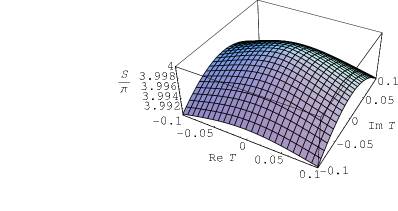
Figure 3: $\mathcal{S}/\pi$ as a function of $T$ for $Y^{0}=1$, $\beta=-1/2$, $a=1$ in the BPS case. The left graph is a cross section along the positive $T$ semi-axis through the surface in the right graph.

Inserting the non-BPS solution (3.23) into (3.11) yields the entropy

$$\begin{split}\frac{\mathcal{S}}{\pi(Y^{0})^{2}}&=\frac{1}{4\pi\left(\beta T^{2}(\log T+1)-2\pi\operatorname{Re}a\right)^{4}}\\ &\quad\Biggl{[}\frac{1}{\beta T^{2}+4\pi\operatorname{Re}a}\Biggl{(}\beta T^{2}(2\log T+3)^{3}\left(\beta T^{2}+4\pi\operatorname{Re}a\right)^{5}\\ &\qquad-{}\Bigr{(}\beta^{2}T^{4}\left(-9\beta T^{2}+4\left(a\pi-\beta T^{2}\right)(\log T)^{2}+4\left(2a\pi-3\beta T^{2}\right)\log T+4a\pi\right)\\ &\qquad-8\pi\beta\left.\operatorname{Re}a\,T^{2}\left(5\beta T^{2}(\log T)^{2}+2\left(7\beta T^{2}+a\pi\right)\log T+2\left(5\beta T^{2}+a\pi\right)\right)\right.\\ &\qquad-32\pi^{3}(\operatorname{Re}a)^{3}+16\pi^{2}(\operatorname{Re}a)^{2}\left(-4\beta T^{2}(\log T)^{2}-7\beta T^{2}-10\beta T^{2}\log T+a\pi\right)\\ &\qquad+4\pi\bar{a}\left(\beta T^{2}(\log T+1)-2\pi\operatorname{Re}a\right)^{2}\Bigr{)}^{2}\Biggr{)}-8\left(\beta T^{2}(\log T+1)-2\pi\operatorname{Re}a\right)^{5}\Biggr{]}\\ &=4\operatorname{Re}a+\frac{\beta}{\pi}T^{2}\left(32(\log T)^{3}+144(\log T)^{2}+214\log T+106\right)+\mathcal{O}(T^{3})\,,\end{split}$$ (5.3)

again in agreement with (2.52),

$$\begin{split}\mathcal{S}_{\text{non-BPS}}&=\pi\lvert Y^{0}\rvert^{2}\mathrm{e}^{-G(z,\bar{z})}\left(1+4\frac{g_{z\bar{z}}^{3}}{\lvert C_{111}\rvert^{2}}\right)\\ &=2\lvert Y^{0}\rvert^{2}\left(2\pi\operatorname{Re}a-\beta\lvert T\rvert^{2}\log\lvert T\rvert-\beta(\operatorname{Re}T)^{2}\right)\\ &\hskip-14.22636pt\left(1+\beta\lvert T\rvert^{2}\frac{\left(\beta\lvert T\rvert^{2}(1-2\log\lvert T\rvert)+2\beta(\operatorname{Re}T)^{2}\,(1+2\log\lvert T\rvert)+4\pi\operatorname{Re}a\,(3+2\log\lvert T\rvert)\right)^{3}}{4\left(2\pi\operatorname{Re}a-\beta\lvert T\rvert^{2}\log\lvert T\rvert-\beta(\operatorname{Re}T)^{2}\right)^{4}}\right).\end{split}$$ (5.4)

In contrast to the BPS case, $\mathcal{S}$ attains for constant $Y^{0}$ a local minimum at the conifold point. There exists, however, also a local maximum around $T\approx 0.05$ (Fig. 4). As mentioned at the end of the previous section, this point is an attractor, provided that one can still trust the prepotential (2.53) there. If we keep $Y^{0}$ constant as in [17], the maximal value of the non-BPS entropy is higher than that of the BPS entropy. Therefore, the corresponding non-supersymmetric flux vacuum is entropically favored.

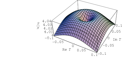
Figure 4: $\mathcal{S}/\pi$ as a function of $T$ for $Y^{0}=1$, $\beta=-1/2$, $a=1$ in the non-BPS case, similarly to Fig. 3.

References

- [1] S. Ferrara, R. Kallosh and A. Strominger, extremal black holes, Phys. Rev. D52 (1995) 5412–5416 [hep-th/9508072].
- [2] A. Strominger, Macroscopic entropy of extremal black holes, Phys. Lett. B383 (1996) 39–43 [hep-th/9602111].
- [3] S. Ferrara and R. Kallosh, Supersymmetry and attractors, Phys. Rev. D54 (1996) 1514–1524 [hep-th/9602136].
- [4] S. Ferrara and R. Kallosh, Universality of supersymmetric attractors, Phys. Rev. D54 (1996) 1525–1534 [hep-th/9603090].
- [5] S. Ferrara, G. W. Gibbons and R. Kallosh, Black holes and critical points in moduli space, Nucl. Phys. B500 (1997) 75–93 [hep-th/9702103].
- [6] G. W. Gibbons, “Supergravity vacua and solitons.” In: Duality and Supersymmetric Theories, D. I. Olive and P. C. West eds., Cambridge, 1997, p. 267.
- [7] K. Goldstein, N. Iizuka, R. P. Jena and S. P. Trivedi, Non-supersymmetric attractors, Phys. Rev. D72 (2005) 124021 [hep-th/0507096].
- [8] R. Kallosh, New attractors, JHEP 12 (2005) 022 [hep-th/0510024].
- [9] R. Kallosh, N. Sivanandam and M. Soroush, The non-BPS black hole attractor equation, JHEP 03 (2006) 060 [hep-th/0602005].
- [10] S. Bellucci, S. Ferrara and A. Marrani, On some properties of the attractor equations, Phys. Lett. B635 (2006) 172–179 [hep-th/0602161].
- [11] A. Sen, Black hole entropy function and the attractor mechanism in higher derivative gravity, JHEP 09 (2005) 038 [hep-th/0506177].
- [12] A. Sen, Entropy function for heterotic black holes, JHEP 03 (2006) 008 [hep-th/0508042].
- [13] B. Sahoo and A. Sen, Higher derivative corrections to non-supersymmetric extremal black holes in supergravity, hep-th/0603149.
- [14] P. Candelas, X. de la Ossa, P. S. Green and L. Parkes, A pair of Calabi–Yau manifolds as an exactly soluble superconformal theory, Nucl. Phys. B359 (1991) 21–74.
- [15] P. K. Tripathy and S. P. Trivedi, Non-supersymmetric attractors in string theory, JHEP 03 (2006) 022 [hep-th/0511117].
- [16] H. Ooguri, C. Vafa and E. P. Verlinde, Hartle–Hawking wave-function for flux compactifications, Lett. Math. Phys. 74 (2005) 311–342 [hep-th/0502211].
- [17] S. Gukov, K. Saraikin and C. Vafa, The entropic principle and asymptotic freedom, Phys. Rev. D73 (2006) 066010 [hep-th/0509109].
- [18] K. Behrndt et al., Classical and quantum supersymmetric black holes, Nucl. Phys. B488 (1997) 236–260 [hep-th/9610105].
- [19] G. L. Cardoso, D. Lüst and J. Perz, Entropy maximization in the presence of higher-curvature interactions, JHEP 05 (2006) 028 [hep-th/0603211].
- [20] B. Fiol, On the critical points of the entropic principle, JHEP 03 (2006) 054 [hep-th/0602103].
- [21] G. L. Cardoso, B. de Wit and S. Mahapatra. In preparation.
- [22] B. de Wit, P. G. Lauwers, R. Philippe, S. Q. Su and A. Van Proeyen, Gauge and matter fields coupled to supergravity, Phys. Lett. B134 (1984) 37.
- [23] B. de Wit and A. Van Proeyen, Potentials and symmetries of general gauged supergravity-Yang–Mills models, Nucl. Phys. B245 (1984) 89.
- [24] B. de Wit, P. G. Lauwers and A. Van Proeyen, Lagrangians of supergravity-matter systems, Nucl. Phys. B255 (1985) 569.
- [25] A. Strominger, Special geometry, Commun. Math. Phys. 133 (1990) 163–180.
- [26] L. Castellani, R. D’Auria and S. Ferrara, Special Kähler geometry: An intrinsic formulation from space-time supersymmetry, Phys. Lett. B241 (1990) 57.
- [27] L. Castellani, R. D’Auria and S. Ferrara, Special geometry without special coordinates, Class. Quant. Grav. 7 (1990) 1767–1790.
- [28] P. Candelas and X. de la Ossa, Moduli space of Calabi–Yau manifolds, Nucl. Phys. B355 (1991) 455–481.
- [29] R. D’Auria, S. Ferrara and P. Fré, Special and quaternionic isometries: General couplings in supergravity and the scalar potential, Nucl. Phys. B359 (1991) 705–740.
- [30] A. Ceresole, R. D’Auria and S. Ferrara, The symplectic structure of supergravity and its central extension, Nucl. Phys. Proc. Suppl. 46 (1996) 67–74 [hep-th/9509160].
- [31] B. de Wit, symplectic reparametrizations in a chiral background, Fortsch. Phys. 44 (1996) 529–538 [hep-th/9603191].
- [32] A. Giryavets, New attractors and area codes, JHEP 03 (2006) 020 [hep-th/0511215].
- [33] M. Alishahiha and H. Ebrahim, New attractor, entropy function and black hole partition function, hep-th/0605279.